跳到论文正文
W Papers独立论文阅读器 arXiv:2105.08283 论文正文 计算阅读时间 · 0%
引用这篇论文根据当前论文元数据生成,正式投稿前建议核对。


License: CC BY 4.0
arXiv:2105.08283v1 [quant-ph] 18 May 2021

Non-Relativistic Scenario of a Free Particle in an Infinite Cylindrical Potential Well

Pratik Adarsh Affiliation: Department of Physics, Indian Institute of Technology Bhilai, GEC Campus, Sejbahar, Raipur, Chhattisgarh 492015, India    Sabyasachi Ghosh Affiliation: Department of Physics, Indian Institute of Technology Bhilai, GEC Campus, Sejbahar, Raipur, Chhattisgarh 492015, India
Abstract

There are various types of infinite potential well problems occurring in elementary quantum mechanics formalism. The infinite square well (one dimensional), cubical box and, spherical well are quite common in textbooks. In this paper, we consider a rather uncommon potential well, infinite cylindrical well, and try to find its energy eigenvalues and eigenfunctions using Schrödinger equation. These results are also derived in the paper[1]. But our approach here is to elaborate every step just the way Griffiths did in his book[2] for hydrogen atom, using spherical potential well. We also plot some radial wavefunctions and density plots.

\justify

1 Introduction

In infinite spherical potential well, we readily solve the time-independent Schrödinger equation to get energy eigenvalues and eigenfunctions. In this problem of infinite cylindrical well, we proceed with the same approach by solving the time-independent Schrödinger equation in cylindrical coordinates.
The motivation is to see how cylindrical symmetry differs from spherical one and to what extend its analytical solutions are possible in the most general way.

2 The Problem

Refer to caption
Figure 1: Infinite cylindrical well.

We have a particle inside a cylindrical-shaped well for which the potential is zero inside the boundaries but infinite at and outside the boundaries.

The dimensional attributes of the well are:
Height of the cylinder = HH
Radius of the cylinder = aa
With these we have to solve the time-independent Schrödinger equation:

−ℏ22​m​∇2ψ+V​ψ=E​ψ{\frac{-{\hbar}^{2}}{2m}}{{\nabla}^{2}}{\psi}+{V\psi}=E\psi

3 The Approach

3.1 Separation of Variables

The Laplacian in cylindrical polar coordinates is:

∇2=1r​∂∂r​(r​∂∂r)+1r2​∂2∂ϕ2+∂2∂z2{\nabla^{2}}={\frac{1}{r}}{\frac{\partial}{\partial r}}\left({r}\frac{\partial}{\partial r}\right)+{\frac{1}{r^{2}}}{\frac{\partial^{2}}{\partial\phi^{2}}}+\frac{\partial^{2}}{\partial z^{2}}

The wavefunction is zero outside the well, so the Schrödinger equation inside(V=0V=0) the well reads:

−ℏ22​m​[1r​∂∂r​(r​∂ψ∂r)+1r2​∂2∂ϕ2+∂2ψ∂z2]=E​ψ\frac{-\hbar^{2}}{2m}\left[\frac{1}{r}\frac{\partial}{\partial r}\left(r\frac{\partial\psi}{\partial r}\right)+\frac{1}{r^{2}}\frac{\partial^{2}}{\partial\phi^{2}}+\frac{\partial^{2}\psi}{\partial z^{2}}\right]=E\psi (3.1.1)

We let the solutions separable into products:

ψ⁡(r,ϕ,z)=ψr​ϕ​(r,ϕ)​ψz​(z)\psi(r,\phi,z)=\psi_{r\phi}(r,\phi)\psi_{z}(z)

Substituting this into equation 3.1.1,we have

−ℏ22​m​[ψzr​∂∂r​(r​∂ψr​ϕ∂r)+ψzr2​∂2ψr​ϕ∂ϕ2+ψr​ϕ​∂2ψz∂z2]=E​ψr​ϕ​ψz\frac{-\hbar^{2}}{2m}\left[\frac{\psi_{z}}{r}\frac{\partial}{\partial r}\left(r\frac{\partial\psi_{r\phi}}{\partial r}\right)+\frac{\psi_{z}}{r^{2}}\frac{\partial^{2}\psi_{r\phi}}{\partial\phi^{2}}+\psi_{r\phi}\frac{\partial^{2}\psi_{z}}{\partial z^{2}}\right]=E\psi_{r\phi}\psi_{z} (3.1.2)

Rearranging terms, we get

1ψr​ϕ​[1r​∂ψr​ϕ∂r+∂2Ψr​ϕ∂r2+1r2​∂2ψr​ϕ∂ϕ2]⏟depends on ​r​ and ​ϕ+1ψz​[d2​ψzd​z2]⏟depends on ​z=−2​m​Eℏ2\underbrace{\frac{1}{\psi_{r\phi}}\left[\frac{1}{r}\frac{\partial\psi_{r\phi}}{\partial r}+\frac{\partial^{2}\Psi_{r\phi}}{\partial r^{2}}+\frac{1}{r^{2}}\frac{\partial^{2}\psi_{r\phi}}{\partial\phi^{2}}\right]}_{\text{depends on }r\text{ and }\phi}+\underbrace{\frac{1}{\psi_{z}}\left[\frac{d^{2}\psi_{z}}{dz^{2}}\right]}_{\text{depends on }z}=-\frac{2mE}{\hbar^{2}} (3.1.3)

In the L.H.S of equation 3.1.3, the first term depends only on rr and ϕ\phi. Whereas the second term depends only on zz. So we let the first term equals some factor A1A_{1}(say)and the second term equals to some another factor A2A_{2}. With these, the equation 3.1.3 reads as:

A1+A2=−2​m​Eℏ2A_{1}+A_{2}=\frac{-2mE}{\hbar^{2}} (3.1.4)

This equation 3.1.4 is the main equation that would give us the energy eigenvalues for the system. Our aim would be now to find these factors, A1A_{1} and A2A_{2}.
Coming back to equation 3.1.3, we write the first term on the L.H.S as:

1r​∂ψr​ϕ∂r+∂2Ψr​ϕ∂r2+1r2​∂2ψr​ϕ∂ϕ2=A1​ψr​ϕ\frac{1}{r}\frac{\partial\psi_{r\phi}}{\partial r}+\frac{\partial^{2}\Psi_{r\phi}}{\partial r^{2}}+\frac{1}{r^{2}}\frac{\partial^{2}\psi_{r\phi}}{\partial\phi^{2}}=A_{1}\psi_{r\phi} (3.1.5)

This is just another partial differential equation we have to solve for proceeding in the right direction. We let the solutions separable like previously:

ψr​ϕ​(r,ϕ)=R⁡(r)​X​(ϕ)\psi_{r\phi}(r,\phi)=R(r)X(\phi)

Substituting this into equation 3.1.5, we have

Xr​d​Rd​r+X​d2​Rd​r2+Rr2​d2​Xd​ϕ2=A1​R​X\frac{X}{r}\frac{dR}{dr}+X\frac{d^{2}R}{dr^{2}}+\frac{R}{r^{2}}\frac{d^{2}X}{d\phi^{2}}=A_{1}RX (3.1.6)

Rearranging terms, we get

[rR​d​Rd​r+r2R​d2​Rd​r2−A1​r2]⏟depends on ​r+[1X​d2​Xd​ϕ2]⏟depends on ​ϕ=0\underbrace{\left[\frac{r}{R}\frac{dR}{dr}+\frac{r^{2}}{R}\frac{d^{2}R}{dr^{2}}-A_{1}r^{2}\right]}_{\text{depends on }r}+\underbrace{\left[\frac{1}{X}\frac{d^{2}X}{d\phi^{2}}\right]}_{\text{depends on }\phi}=0 (3.1.7)

The first term on L.H.S of the equation 3.1.7 depends only on rr and the second term depends only on ϕ\phi. So we let the first term equals to some factor BB(say), then obviously the second term equals to −B-B.
With these attributes, we have:

rR​d​Rd​r+r2R​d2​Rd​r2−A1​r2=B\frac{r}{R}\frac{dR}{dr}+\frac{r^{2}}{R}\frac{d^{2}R}{dr^{2}}-A_{1}r^{2}=B (3.1.8)
1X​d2​Xd​ϕ2=−B\frac{1}{X}\frac{d^{2}X}{d\phi^{2}}=-B (3.1.9)

And from equations 3.1.3 and 3.1.4

1ψz​[d2​ψzd​z2]=A2\frac{1}{\psi_{z}}\left[\frac{d^{2}\psi_{z}}{dz^{2}}\right]=A_{2} (3.1.10)

3.2 The Radial Equation

We can rewrite equation 3.1.8 as:

dd​r​(r​R′​(r))+[−A1−Br2]​r​R​(r)=0​ (Strum-Liouville Equation)\frac{d}{dr}\left(rR^{\prime}(r)\right)+\left[-A_{1}-\frac{B}{r^{2}}\right]rR(r)=0\textit{ (Strum-Liouville Equation)} (3.2.1)

Its solution is:

R⁡(r)=C1​JB​(−i​A1​r)+C2​YB​(−i​A1​r)R(r)=C_{1}J_{\mathchoice{\raisebox{0.0pt}{\resizebox{437263}{327680}{\hbox{\raisebox{0.0pt}{$\displaystyle\sqrt{B}$}}}}}{\raisebox{0.0pt}{\resizebox{437263}{327680}{\hbox{\raisebox{0.0pt}{$\textstyle\sqrt{B}$}}}}}{\raisebox{0.0pt}{\resizebox{387787}{327680}{\hbox{\raisebox{0.0pt}{$\scriptstyle\sqrt{B}$}}}}}{\raisebox{0.0pt}{\resizebox{387786}{327680}{\hbox{\raisebox{0.0pt}{$\scriptscriptstyle\sqrt{B}$}}}}}}\left(-i\sqrt{A_{1}}r\right)+C_{2}Y_{\mathchoice{\raisebox{0.0pt}{\resizebox{437263}{327680}{\hbox{\raisebox{0.0pt}{$\displaystyle\sqrt{B}$}}}}}{\raisebox{0.0pt}{\resizebox{437263}{327680}{\hbox{\raisebox{0.0pt}{$\textstyle\sqrt{B}$}}}}}{\raisebox{0.0pt}{\resizebox{387787}{327680}{\hbox{\raisebox{0.0pt}{$\scriptstyle\sqrt{B}$}}}}}{\raisebox{0.0pt}{\resizebox{387786}{327680}{\hbox{\raisebox{0.0pt}{$\scriptscriptstyle\sqrt{B}$}}}}}}\left(-i\sqrt{A_{1}}r\right) (3.2.2)

Where JJ and YY are Bessel functions of first and second kind respectively. Equation 3.2.2 gives us the radial wavefunction. We have to solve it with appropriate boundary conditions. We would do this later, now the main task is to simplify it with this simple view:
For r→ 0r\,\to\,0, equation 3.2.2 reads as:

R⁡(0)=C1​JB​(0)+C2​YB​(0)R(0)=C_{1}J_{\mathchoice{\raisebox{0.0pt}{\resizebox{437263}{327680}{\hbox{\raisebox{0.0pt}{$\displaystyle\sqrt{B}$}}}}}{\raisebox{0.0pt}{\resizebox{437263}{327680}{\hbox{\raisebox{0.0pt}{$\textstyle\sqrt{B}$}}}}}{\raisebox{0.0pt}{\resizebox{387787}{327680}{\hbox{\raisebox{0.0pt}{$\scriptstyle\sqrt{B}$}}}}}{\raisebox{0.0pt}{\resizebox{387786}{327680}{\hbox{\raisebox{0.0pt}{$\scriptscriptstyle\sqrt{B}$}}}}}}\left(0\right)+C_{2}Y_{\mathchoice{\raisebox{0.0pt}{\resizebox{437263}{327680}{\hbox{\raisebox{0.0pt}{$\displaystyle\sqrt{B}$}}}}}{\raisebox{0.0pt}{\resizebox{437263}{327680}{\hbox{\raisebox{0.0pt}{$\textstyle\sqrt{B}$}}}}}{\raisebox{0.0pt}{\resizebox{387787}{327680}{\hbox{\raisebox{0.0pt}{$\scriptstyle\sqrt{B}$}}}}}{\raisebox{0.0pt}{\resizebox{387786}{327680}{\hbox{\raisebox{0.0pt}{$\scriptscriptstyle\sqrt{B}$}}}}}}\left(0\right)

But we know that

YB​(0)→∞Y_{\mathchoice{\raisebox{0.0pt}{\resizebox{437263}{327680}{\hbox{\raisebox{0.0pt}{$\displaystyle\sqrt{B}$}}}}}{\raisebox{0.0pt}{\resizebox{437263}{327680}{\hbox{\raisebox{0.0pt}{$\textstyle\sqrt{B}$}}}}}{\raisebox{0.0pt}{\resizebox{387787}{327680}{\hbox{\raisebox{0.0pt}{$\scriptstyle\sqrt{B}$}}}}}{\raisebox{0.0pt}{\resizebox{387786}{327680}{\hbox{\raisebox{0.0pt}{$\scriptscriptstyle\sqrt{B}$}}}}}}\left(0\right)\,\to\,\infty
JB​(0)=0J_{\mathchoice{\raisebox{0.0pt}{\resizebox{437263}{327680}{\hbox{\raisebox{0.0pt}{$\displaystyle\sqrt{B}$}}}}}{\raisebox{0.0pt}{\resizebox{437263}{327680}{\hbox{\raisebox{0.0pt}{$\textstyle\sqrt{B}$}}}}}{\raisebox{0.0pt}{\resizebox{387787}{327680}{\hbox{\raisebox{0.0pt}{$\scriptstyle\sqrt{B}$}}}}}{\raisebox{0.0pt}{\resizebox{387786}{327680}{\hbox{\raisebox{0.0pt}{$\scriptscriptstyle\sqrt{B}$}}}}}}\left(0\right)=0

This means that the radial wavefunction, R⁡(0)R(0) diverges on the axis of the well. In other words this implies that it’s a non-normalizable wavefunction.
Therefore we must have C2=0C_{2}=0.
So now our radial wavefunction, equation 3.2.2 becomes:

R⁡(r)=C1​JB​(−i​A1​r)R(r)=C_{1}J_{\mathchoice{\raisebox{0.0pt}{\resizebox{437263}{327680}{\hbox{\raisebox{0.0pt}{$\displaystyle\sqrt{B}$}}}}}{\raisebox{0.0pt}{\resizebox{437263}{327680}{\hbox{\raisebox{0.0pt}{$\textstyle\sqrt{B}$}}}}}{\raisebox{0.0pt}{\resizebox{387787}{327680}{\hbox{\raisebox{0.0pt}{$\scriptstyle\sqrt{B}$}}}}}{\raisebox{0.0pt}{\resizebox{387786}{327680}{\hbox{\raisebox{0.0pt}{$\scriptscriptstyle\sqrt{B}$}}}}}}\left(-i\sqrt{A_{1}}r\right) (3.2.3)

We will return to this equation soon for calculating A1A_{1}, to plug in the equation 3.1.4 and getting the energy eigenvalues. But first, we have to find what BB corresponds and of course, we also have to find A2A_{2}.

3.3 The Angular Equation

The equation 3.1.9 is:

1X​d2​Xd​ϕ2=−B\frac{1}{X}\frac{d^{2}X}{d\phi^{2}}=-B

Its solution can be written as:

X⁡(ϕ)=C3​exp⁡(i​B​ϕ)+C4​exp⁡(−i​B​ϕ)X(\phi)=C_{3}\exp\left(i\sqrt{B}\phi\right)+C_{4}\exp\left(-i\sqrt{B}\phi\right) (3.3.1)

For rotational symmetry, we must have:

X⁡(ϕ+2​π)=X⁡(ϕ)X(\phi+2\pi)=X(\phi)
⟹C3​exp⁡(i​B​(ϕ+2​π))+C4​exp⁡(−i​B​(ϕ+2​π))=C3​exp⁡(i​B​ϕ)+C4​exp⁡(−i​B​ϕ)\implies C_{3}\exp\left(i\sqrt{B}(\phi+2\pi)\right)+C_{4}\exp\left(-i\sqrt{B}(\phi+2\pi)\right)=C_{3}\exp\left(i\sqrt{B}\phi\right)+C_{4}\exp\left(-i\sqrt{B}\phi\right)

Simplifying and equating real and imaginary parts, we get:

(C3+C4)​[cos⁡(B​ϕ+2​π​B)]=(C3+C4)​cos⁡(B​ϕ)\left(C_{3}+C_{4}\right)\left[\cos(\sqrt{B}\phi+2\pi\sqrt{B})\right]=\left(C_{3}+C_{4}\right)\cos(\sqrt{B}\phi)

and

(C3−C4)​[sin⁡(B​ϕ+2​π​B)]=(C3−C4)​sin⁡(B​ϕ)\left(C_{3}-C_{4}\right)\left[\sin(\sqrt{B}\phi+2\pi\sqrt{B})\right]=\left(C_{3}-C_{4}\right)\sin(\sqrt{B}\phi)

Therefore B\sqrt{B} is an integer, for C3+C4≠0C_{3}+C_{4}\neq 0 and C3≠C4C_{3}\neq C_{4}. Hence we have

B=nϕ=0,1,2,…\sqrt{B}=n_{\phi}=0,1,2,... (3.3.2)

where nϕn_{\phi} denotes a quantum number associated with azimuthal angle.

3.4 The Equation along Z Direction

The equation 3.1.10 is:

1ψz​[d2​ψzd​z2]=A2\frac{1}{\psi_{z}}\left[\frac{d^{2}\psi_{z}}{dz^{2}}\right]=A_{2}

Its solution can be written as:

ψz​(z)=C5​exp⁡(i​z​2​m​Eℏ2+A1)+C6​exp⁡(−i​z​2​m​Eℏ2+A1)\psi_{z}(z)=C_{5}\exp\left(iz\sqrt{\frac{2mE}{\hbar^{2}}+A_{1}}\right)+C_{6}\exp\left(-iz\sqrt{\frac{2mE}{\hbar^{2}}+A_{1}}\right) (3.4.1)

Now we have the following boundary conditions:

  1. (i.)

    ψz​(0)=0\psi_{z}(0)=0

  2. (ii.)

    ψz​(H)=0\psi_{z}(H)=0

Imposing the first condition on the equation 3.4.1, we have:

C6=−C5C_{6}=-C_{5}

With this and by second boundary condition, the equation 3.4.1 becomes:

C5​exp⁡(i​z​2​m​Eℏ2+A1)−C5​exp⁡(−i​z​2​m​Eℏ2+A1)=0C_{5}\exp\left(iz\sqrt{\frac{2mE}{\hbar^{2}}+A_{1}}\right)-C_{5}\exp\left(-iz\sqrt{\frac{2mE}{\hbar^{2}}+A_{1}}\right)=0
⟹2​i​C5​[sin⁡(H​2​m​Eℏ2+A1)]=0\implies 2iC_{5}\left[\sin\left(H\sqrt{\frac{2mE}{\hbar^{2}}+A_{1}}\right)\right]=0
⟹H2​m​Eℏ2+A1=nzπ;nz=1,2,3,…\implies H\sqrt{\frac{2mE}{\hbar^{2}}+A_{1}}=n_{z}\pi\hskip 5.0pt;n_{z}=1,2,3,... (3.4.2)

Where nzn_{z} denotes a quantum number associated with z-direction.
Using equations 3.4.2 and 3.1.4, we have:

A2=−nz2​π2H2A_{2}=\frac{-n_{z}^{2}\pi^{2}}{H^{2}} (3.4.3)

Therefore we have energy expression redefined as:

E=ℏ2​(nz2​π2−A1​H2)2​m​H2E=\frac{\hbar^{2}(n_{z}^{2}\pi^{2}-A_{1}H^{2})}{2mH^{2}} (3.4.4)

3.5 Energy Eigenvalues

With some remaining calculations, we are now very near to get the energy eigenvalues.
It’s now time to return to equation 3.2.3 with the consideration of equation 3.3.2, we have

R⁡(r)=C1​Jnϕ​(−i​A1​r)R(r)=C_{1}J_{\mathchoice{\raisebox{-3.23962pt}{\resizebox{909244}{327680}{\hbox{\raisebox{1.95277pt}{$\displaystyle n_{\phi}$}}}}}{\raisebox{-3.23962pt}{\resizebox{909244}{327680}{\hbox{\raisebox{1.95277pt}{$\textstyle n_{\phi}$}}}}}{\raisebox{-3.37323pt}{\resizebox{858385}{327680}{\hbox{\raisebox{1.42331pt}{$\scriptstyle n_{\phi}$}}}}}{\raisebox{-6.32251pt}{\resizebox{1019006}{327680}{\hbox{\raisebox{1.90553pt}{$\scriptscriptstyle n_{\phi}$}}}}}}\left(-i\sqrt{A_{1}}r\right) (3.5.1)

Imposing the boundary condition

R⁡(a)=0R(a)=0

We get

⟹R⁡(a)=C1​Jnϕ​(−i​A1​a)=0\implies R(a)=C_{1}J_{\mathchoice{\raisebox{-3.23962pt}{\resizebox{909244}{327680}{\hbox{\raisebox{1.95277pt}{$\displaystyle n_{\phi}$}}}}}{\raisebox{-3.23962pt}{\resizebox{909244}{327680}{\hbox{\raisebox{1.95277pt}{$\textstyle n_{\phi}$}}}}}{\raisebox{-3.37323pt}{\resizebox{858385}{327680}{\hbox{\raisebox{1.42331pt}{$\scriptstyle n_{\phi}$}}}}}{\raisebox{-6.32251pt}{\resizebox{1019006}{327680}{\hbox{\raisebox{1.90553pt}{$\scriptscriptstyle n_{\phi}$}}}}}}\left(-i\sqrt{A_{1}}a\right)=0
⟹A1=−(jnϕ,nr)2a2;nr=1,2,3,…\implies A_{1}=\frac{-(j_{\mathchoice{\raisebox{-3.23962pt}{\resizebox{2150839}{327680}{\hbox{\raisebox{1.95277pt}{$\displaystyle n_{\phi},n_{r}$}}}}}{\raisebox{-3.23962pt}{\resizebox{2150839}{327680}{\hbox{\raisebox{1.95277pt}{$\textstyle n_{\phi},n_{r}$}}}}}{\raisebox{-3.37323pt}{\resizebox{2076756}{327680}{\hbox{\raisebox{1.42331pt}{$\scriptstyle n_{\phi},n_{r}$}}}}}{\raisebox{-6.32251pt}{\resizebox{2457425}{327680}{\hbox{\raisebox{1.90553pt}{$\scriptscriptstyle n_{\phi},n_{r}$}}}}}})^{2}}{a^{2}}\hskip 5.0pt;n_{r}=1,2,3,... (3.5.2)

Where nrn_{r} denotes a quantum number associated with radial solution and jnϕ,nrj_{\mathchoice{\raisebox{-3.23962pt}{\resizebox{2150839}{327680}{\hbox{\raisebox{1.95277pt}{$\displaystyle n_{\phi},n_{r}$}}}}}{\raisebox{-3.23962pt}{\resizebox{2150839}{327680}{\hbox{\raisebox{1.95277pt}{$\textstyle n_{\phi},n_{r}$}}}}}{\raisebox{-3.37323pt}{\resizebox{2076756}{327680}{\hbox{\raisebox{1.42331pt}{$\scriptstyle n_{\phi},n_{r}$}}}}}{\raisebox{-6.32251pt}{\resizebox{2457425}{327680}{\hbox{\raisebox{1.90553pt}{$\scriptscriptstyle n_{\phi},n_{r}$}}}}}} denotes nrt​hn_{r}^{th} root of Bessel function JnϕJ_{\mathchoice{\raisebox{-3.23962pt}{\resizebox{909244}{327680}{\hbox{\raisebox{1.95277pt}{$\displaystyle n_{\phi}$}}}}}{\raisebox{-3.23962pt}{\resizebox{909244}{327680}{\hbox{\raisebox{1.95277pt}{$\textstyle n_{\phi}$}}}}}{\raisebox{-3.37323pt}{\resizebox{858385}{327680}{\hbox{\raisebox{1.42331pt}{$\scriptstyle n_{\phi}$}}}}}{\raisebox{-6.32251pt}{\resizebox{1019006}{327680}{\hbox{\raisebox{1.90553pt}{$\scriptscriptstyle n_{\phi}$}}}}}}
Putting this equation 3.5.2 into equation 3.4.4, we have the final expression for energy eigenvalues as:

Enr,nϕ,nz=ℏ2​[nz2​a2​π2+(jnϕ,nr)2​H2]2​m​a2​H2\boxed{E_{\mathchoice{\raisebox{-3.23962pt}{\resizebox{3408465}{327680}{\hbox{\raisebox{1.95277pt}{$\displaystyle n_{r},n_{\phi},n_{z}$}}}}}{\raisebox{-3.23962pt}{\resizebox{3408465}{327680}{\hbox{\raisebox{1.95277pt}{$\textstyle n_{r},n_{\phi},n_{z}$}}}}}{\raisebox{-3.37323pt}{\resizebox{3311487}{327680}{\hbox{\raisebox{1.42331pt}{$\scriptstyle n_{r},n_{\phi},n_{z}$}}}}}{\raisebox{-6.32251pt}{\resizebox{3918748}{327680}{\hbox{\raisebox{1.90553pt}{$\scriptscriptstyle n_{r},n_{\phi},n_{z}$}}}}}}=\frac{\hbar^{2}\left[n_{z}^{2}a^{2}\pi^{2}+(j_{\mathchoice{\raisebox{-3.23962pt}{\resizebox{2150839}{327680}{\hbox{\raisebox{1.95277pt}{$\displaystyle n_{\phi},n_{r}$}}}}}{\raisebox{-3.23962pt}{\resizebox{2150839}{327680}{\hbox{\raisebox{1.95277pt}{$\textstyle n_{\phi},n_{r}$}}}}}{\raisebox{-3.37323pt}{\resizebox{2076756}{327680}{\hbox{\raisebox{1.42331pt}{$\scriptstyle n_{\phi},n_{r}$}}}}}{\raisebox{-6.32251pt}{\resizebox{2457425}{327680}{\hbox{\raisebox{1.90553pt}{$\scriptscriptstyle n_{\phi},n_{r}$}}}}}})^{2}H^{2}\right]}{2ma^{2}H^{2}}} (3.5.3)

Where

nr\displaystyle n_{r} =1,2,3,…\displaystyle=1,2,3,...
nϕ\displaystyle n_{\phi} =0,1,2,…\displaystyle=0,1,2,...
nz\displaystyle n_{z} =1,2,3,…\displaystyle=1,2,3,...

3.6 The Eigenfunctions

We started with separable solutions of the Schrödinger’s equation 3.1.1 as:

ψ⁡(r,ϕ,z)=ψr​ϕ​(r,ϕ)​ψz​(z)=R⁡(r)​X​(ϕ)​ψz​(z)\psi(r,\phi,z)=\psi_{r\phi}(r,\phi)\psi_{z}(z)=R(r)X(\phi)\psi_{z}(z) (3.6.1)

Now we will find R⁡(r)R(r), X⁡(ϕ)X(\phi) and ψz​(z)\psi_{z}(z) separately and put them back into the equation 3.6.1 to get the complete eigenfunctions.

The Normalization Technique

Before finding the wavefunctions, we emphasize that how normalization can be done separately for each of them.
In cylindrical coordinates, we have elementary volume as:

d​V=r​d​r​d​ϕ​d​zdV=rdrd\phi dz

So normalization of wavefunction in the view of equation 3.6.1 becomes

∭Vψ⁡(r,ϕ,z)​ψ∗​(r,ϕ,z)​r​𝑑r​𝑑ϕ​𝑑z=∫0aR⁡(r)​R∗​(r)​r​𝑑r​∫02​πX⁡(ϕ)​X∗​(ϕ)​𝑑ϕ​∫0Hψz​(z)​ψz∗​(z)​𝑑z=1\iiint_{V}\psi(r,\phi,z)\psi^{*}(r,\phi,z){rdrd\phi dz}=\int_{0}^{a}R(r)R^{*}(r)rdr\int_{0}^{2\pi}X(\phi)X^{*}(\phi)d\phi\int_{0}^{H}\psi_{z}(z)\psi_{z}^{*}(z)dz=1

We can normalize each wavefunctions separately as follows:

  1. (i.)
    ∫0aR⁡(r)​R∗​(r)​r​𝑑r=1\int_{0}^{a}R(r)R^{*}(r)rdr=1 (3.6.2)
  1. (ii.)
    ∫02​πX⁡(ϕ)​X∗​(ϕ)​𝑑ϕ=1\int_{0}^{2\pi}X(\phi)X^{*}(\phi)d\phi=1 (3.6.3)
  1. (iii.)
    ∫0Hψz​(z)​ψz∗​(z)​𝑑z=1\int_{0}^{H}\psi_{z}(z)\psi_{z}^{*}(z)dz=1 (3.6.4)

The Radial wavefunctions

From the equations 3.5.1 and 3.5.2, we have:

R⁡(r)=C1​Jnϕ​[(jnϕ,nr)​ra]R(r)=C_{1}J_{\mathchoice{\raisebox{-3.23962pt}{\resizebox{909244}{327680}{\hbox{\raisebox{1.95277pt}{$\displaystyle n_{\phi}$}}}}}{\raisebox{-3.23962pt}{\resizebox{909244}{327680}{\hbox{\raisebox{1.95277pt}{$\textstyle n_{\phi}$}}}}}{\raisebox{-3.37323pt}{\resizebox{858385}{327680}{\hbox{\raisebox{1.42331pt}{$\scriptstyle n_{\phi}$}}}}}{\raisebox{-6.32251pt}{\resizebox{1019006}{327680}{\hbox{\raisebox{1.90553pt}{$\scriptscriptstyle n_{\phi}$}}}}}}\left[\frac{(j_{\mathchoice{\raisebox{-3.23962pt}{\resizebox{2150839}{327680}{\hbox{\raisebox{1.95277pt}{$\displaystyle n_{\phi},n_{r}$}}}}}{\raisebox{-3.23962pt}{\resizebox{2150839}{327680}{\hbox{\raisebox{1.95277pt}{$\textstyle n_{\phi},n_{r}$}}}}}{\raisebox{-3.37323pt}{\resizebox{2076756}{327680}{\hbox{\raisebox{1.42331pt}{$\scriptstyle n_{\phi},n_{r}$}}}}}{\raisebox{-6.32251pt}{\resizebox{2457425}{327680}{\hbox{\raisebox{1.90553pt}{$\scriptscriptstyle n_{\phi},n_{r}$}}}}}})r}{a}\right] (3.6.5)

To make further calculations easier to follow, we take the following denotations:

nϕ=n​ and ​jnϕ,nr=βn_{\phi}=n\text{ and }j_{\mathchoice{\raisebox{-3.23962pt}{\resizebox{2150839}{327680}{\hbox{\raisebox{1.95277pt}{$\displaystyle n_{\phi},n_{r}$}}}}}{\raisebox{-3.23962pt}{\resizebox{2150839}{327680}{\hbox{\raisebox{1.95277pt}{$\textstyle n_{\phi},n_{r}$}}}}}{\raisebox{-3.37323pt}{\resizebox{2076756}{327680}{\hbox{\raisebox{1.42331pt}{$\scriptstyle n_{\phi},n_{r}$}}}}}{\raisebox{-6.32251pt}{\resizebox{2457425}{327680}{\hbox{\raisebox{1.90553pt}{$\scriptscriptstyle n_{\phi},n_{r}$}}}}}}=\beta

With these, the radial equation 3.6.5 becomes

R⁡(r)=C1​Jn​[β​ra]R(r)=C_{1}J_{n}\left[\frac{\beta{r}}{a}\right] (3.6.6)

Normalizing using equation 3.6.2, we have

C12​∫0aJn2​[β​ra]​r​𝑑r=1C_{1}^{2}\int_{0}^{a}J_{n}^{2}\left[\frac{\beta{r}}{a}\right]rdr=1 (3.6.7)

The indefinite integral has solution as:

∫Jn2​[β​ra]​r​𝑑r=r22​[Jn2​[β​ra]−Jn−1​[β​ra]​Jn+1​[β​ra]]+C\int{J_{n}^{2}\left[\frac{\beta{r}}{a}\right]rdr}=\frac{r^{2}}{2}\left[J_{n}^{2}\left[\frac{\beta{r}}{a}\right]-J_{n-1}\left[\frac{\beta{r}}{a}\right]J_{n+1}\left[\frac{\beta{r}}{a}\right]\right]+C (3.6.8)

where CC is the constant of integration.
With the proper limits of integration, [0,a][0,a] and using Bessel recurrence relation:

Jn−1​(x)+Jn+1​(x)=2​nx​Jn​(x)J_{n-1}(x)+J_{n+1}(x)=2\frac{n}{x}J_{n}(x) (3.6.9)

we have

C1=2a​Jn+1​(β)C_{1}=\frac{\sqrt{2}}{aJ_{\mathchoice{\raisebox{-0.92365pt}{\resizebox{1359090}{327680}{\hbox{\raisebox{0.83334pt}{$\displaystyle n+1$}}}}}{\raisebox{-0.92365pt}{\resizebox{1359090}{327680}{\hbox{\raisebox{0.83334pt}{$\textstyle n+1$}}}}}{\raisebox{-0.64653pt}{\resizebox{1332835}{327680}{\hbox{\raisebox{0.40833pt}{$\scriptstyle n+1$}}}}}{\raisebox{-0.64651pt}{\resizebox{1484005}{327680}{\hbox{\raisebox{0.29166pt}{$\scriptscriptstyle n+1$}}}}}}\left(\beta\right)}

Putting back into equation 3.6.5 and restoring the original denotations, we get the normalized radial wavefunctions as:

R⁡(r)=2a​Jnϕ+1​[jnϕ,nr]​Jnϕ​[(jnϕ,nr)​ra]\boxed{R(r)=\frac{\sqrt{2}}{aJ_{\mathchoice{\raisebox{-2.1644pt}{\resizebox{1475210}{327680}{\hbox{\raisebox{1.95277pt}{$\displaystyle n_{\phi}+1$}}}}}{\raisebox{-2.1644pt}{\resizebox{1475210}{327680}{\hbox{\raisebox{1.95277pt}{$\textstyle n_{\phi}+1$}}}}}{\raisebox{-2.25365pt}{\resizebox{1412160}{327680}{\hbox{\raisebox{1.42331pt}{$\scriptstyle n_{\phi}+1$}}}}}{\raisebox{-4.22408pt}{\resizebox{1595060}{327680}{\hbox{\raisebox{1.90553pt}{$\scriptscriptstyle n_{\phi}+1$}}}}}}\left[j_{\mathchoice{\raisebox{-3.23962pt}{\resizebox{2150839}{327680}{\hbox{\raisebox{1.95277pt}{$\displaystyle n_{\phi},n_{r}$}}}}}{\raisebox{-3.23962pt}{\resizebox{2150839}{327680}{\hbox{\raisebox{1.95277pt}{$\textstyle n_{\phi},n_{r}$}}}}}{\raisebox{-3.37323pt}{\resizebox{2076756}{327680}{\hbox{\raisebox{1.42331pt}{$\scriptstyle n_{\phi},n_{r}$}}}}}{\raisebox{-6.32251pt}{\resizebox{2457425}{327680}{\hbox{\raisebox{1.90553pt}{$\scriptscriptstyle n_{\phi},n_{r}$}}}}}}\right]}J_{\mathchoice{\raisebox{-3.23962pt}{\resizebox{909244}{327680}{\hbox{\raisebox{1.95277pt}{$\displaystyle n_{\phi}$}}}}}{\raisebox{-3.23962pt}{\resizebox{909244}{327680}{\hbox{\raisebox{1.95277pt}{$\textstyle n_{\phi}$}}}}}{\raisebox{-3.37323pt}{\resizebox{858385}{327680}{\hbox{\raisebox{1.42331pt}{$\scriptstyle n_{\phi}$}}}}}{\raisebox{-6.32251pt}{\resizebox{1019006}{327680}{\hbox{\raisebox{1.90553pt}{$\scriptscriptstyle n_{\phi}$}}}}}}\left[\frac{(j_{\mathchoice{\raisebox{-3.23962pt}{\resizebox{2150839}{327680}{\hbox{\raisebox{1.95277pt}{$\displaystyle n_{\phi},n_{r}$}}}}}{\raisebox{-3.23962pt}{\resizebox{2150839}{327680}{\hbox{\raisebox{1.95277pt}{$\textstyle n_{\phi},n_{r}$}}}}}{\raisebox{-3.37323pt}{\resizebox{2076756}{327680}{\hbox{\raisebox{1.42331pt}{$\scriptstyle n_{\phi},n_{r}$}}}}}{\raisebox{-6.32251pt}{\resizebox{2457425}{327680}{\hbox{\raisebox{1.90553pt}{$\scriptscriptstyle n_{\phi},n_{r}$}}}}}})r}{a}\right]} (3.6.10)

The Angular wavefunctions

The angular wavefunctions are given by equation 3.3.1, they are basically two linearly independent angular solutions. But we can compress it to the form:

X⁡(ϕ)=Cp​exp⁡(i​p​ϕ)​; where ​p=±B=±nϕ=0,±1,±2,…X(\phi)=C_{p}\exp(ip\phi)\text{; where }p=\pm\sqrt{B}=\pm n_{\phi}=0,\pm 1,\pm 2,... (3.6.11)

The pp is like another quantum number that would be responsible for state degeneracy. We can normalize 3.6.11 in the view of the equation 3.6.3, we get the normalized angular wavefunctions as:

X⁡(ϕ)=12​π​exp⁡(i​p​ϕ)​ ; ​p=±nϕ=0,±1,±2,…\boxed{X(\phi)=\frac{1}{\sqrt{2\pi}}\exp(ip\phi)\text{ ; }p=\pm n_{\phi}=0,\pm 1,\pm 2,...} (3.6.12)

The wavefunctions along Z-Direction

From subsection 3.4, we have wavefunctions along z-direction as:

ψz​(z)=2​i​C5​[sin⁡(z​2​m​Eℏ2+A1)]\psi_{z}(z)=2iC_{5}\left[\sin\left(z\sqrt{\frac{2mE}{\hbar^{2}}+A_{1}}\right)\right] (3.6.13)

Using the equation 3.4.4, we can rewrite equation 3.6.13 as:

ψz​(z)=2​C5′​sin⁡(nz​π​zH)\psi_{z}(z)=2C_{5}^{\prime}\sin\left(\frac{n_{z}\pi{z}}{H}\right) (3.6.14)

Normalizing in the view of equation 3.6.4, we get the normalized wavefunctions along the z-direction as:

ψz​(z)=[2H]​sin⁡(nz​π​zH)​ ; ​nz=1,2,3,…\boxed{\psi_{z}(z)=\left[\sqrt{\frac{2}{H}}\right]\sin\left(\frac{n_{z}\pi{z}}{H}\right)\text{ ; }n_{z}=1,2,3,...} (3.6.15)

Now using equation 3.6.1, we stack up all the wavefunctions and get the final expression as:

ψnr,nϕ,nz,p=[2π​H​a2]​1Jnϕ+1​[jnϕ,nr]​Jnϕ​[(jnϕ,nr)​ra]​sin⁡[nz​π​zH]​exp⁡(i​p​ϕ)\boxed{\psi_{\mathchoice{\raisebox{-3.23962pt}{\resizebox{4251287}{327680}{\hbox{\raisebox{1.95277pt}{$\displaystyle n_{r},n_{\phi},n_{z},p$}}}}}{\raisebox{-3.23962pt}{\resizebox{4251287}{327680}{\hbox{\raisebox{1.95277pt}{$\textstyle n_{r},n_{\phi},n_{z},p$}}}}}{\raisebox{-3.37323pt}{\resizebox{4117934}{327680}{\hbox{\raisebox{1.42331pt}{$\scriptstyle n_{r},n_{\phi},n_{z},p$}}}}}{\raisebox{-6.32251pt}{\resizebox{4810040}{327680}{\hbox{\raisebox{1.90553pt}{$\scriptscriptstyle n_{r},n_{\phi},n_{z},p$}}}}}}=\left[\sqrt{\frac{2}{\pi{Ha^{2}}}}\right]\frac{1}{J_{\mathchoice{\raisebox{-2.1644pt}{\resizebox{1475210}{327680}{\hbox{\raisebox{1.95277pt}{$\displaystyle n_{\phi}+1$}}}}}{\raisebox{-2.1644pt}{\resizebox{1475210}{327680}{\hbox{\raisebox{1.95277pt}{$\textstyle n_{\phi}+1$}}}}}{\raisebox{-2.25365pt}{\resizebox{1412160}{327680}{\hbox{\raisebox{1.42331pt}{$\scriptstyle n_{\phi}+1$}}}}}{\raisebox{-4.22408pt}{\resizebox{1595060}{327680}{\hbox{\raisebox{1.90553pt}{$\scriptscriptstyle n_{\phi}+1$}}}}}}\left[j_{\mathchoice{\raisebox{-3.23962pt}{\resizebox{2150839}{327680}{\hbox{\raisebox{1.95277pt}{$\displaystyle n_{\phi},n_{r}$}}}}}{\raisebox{-3.23962pt}{\resizebox{2150839}{327680}{\hbox{\raisebox{1.95277pt}{$\textstyle n_{\phi},n_{r}$}}}}}{\raisebox{-3.37323pt}{\resizebox{2076756}{327680}{\hbox{\raisebox{1.42331pt}{$\scriptstyle n_{\phi},n_{r}$}}}}}{\raisebox{-6.32251pt}{\resizebox{2457425}{327680}{\hbox{\raisebox{1.90553pt}{$\scriptscriptstyle n_{\phi},n_{r}$}}}}}}\right]}J_{\mathchoice{\raisebox{-3.23962pt}{\resizebox{909244}{327680}{\hbox{\raisebox{1.95277pt}{$\displaystyle n_{\phi}$}}}}}{\raisebox{-3.23962pt}{\resizebox{909244}{327680}{\hbox{\raisebox{1.95277pt}{$\textstyle n_{\phi}$}}}}}{\raisebox{-3.37323pt}{\resizebox{858385}{327680}{\hbox{\raisebox{1.42331pt}{$\scriptstyle n_{\phi}$}}}}}{\raisebox{-6.32251pt}{\resizebox{1019006}{327680}{\hbox{\raisebox{1.90553pt}{$\scriptscriptstyle n_{\phi}$}}}}}}\left[\frac{(j_{\mathchoice{\raisebox{-3.23962pt}{\resizebox{2150839}{327680}{\hbox{\raisebox{1.95277pt}{$\displaystyle n_{\phi},n_{r}$}}}}}{\raisebox{-3.23962pt}{\resizebox{2150839}{327680}{\hbox{\raisebox{1.95277pt}{$\textstyle n_{\phi},n_{r}$}}}}}{\raisebox{-3.37323pt}{\resizebox{2076756}{327680}{\hbox{\raisebox{1.42331pt}{$\scriptstyle n_{\phi},n_{r}$}}}}}{\raisebox{-6.32251pt}{\resizebox{2457425}{327680}{\hbox{\raisebox{1.90553pt}{$\scriptscriptstyle n_{\phi},n_{r}$}}}}}})r}{a}\right]\sin\left[\frac{n_{z}\pi{z}}{H}\right]\exp(ip\phi)} (3.6.16)

Where

nr\displaystyle n_{r} =1,2,3,…\displaystyle=1,2,3,...
nϕ\displaystyle n_{\phi} =0,1,2,…\displaystyle=0,1,2,...
nz\displaystyle n_{z} =1,2,3,…\displaystyle=1,2,3,...
p\displaystyle p =±nϕ\displaystyle=\pm n_{\phi}

4 Plots

4.1 Radial Wavefunctions

Refer to caption
Figure 2: Some Radial Wavefunctions Rnr,nϕR_{\mathchoice{\raisebox{-3.23962pt}{\resizebox{2150839}{327680}{\hbox{\raisebox{1.95277pt}{$\displaystyle n_{r},n_{\phi}$}}}}}{\raisebox{-3.23962pt}{\resizebox{2150839}{327680}{\hbox{\raisebox{1.95277pt}{$\textstyle n_{r},n_{\phi}$}}}}}{\raisebox{-3.37323pt}{\resizebox{2076756}{327680}{\hbox{\raisebox{1.42331pt}{$\scriptstyle n_{r},n_{\phi}$}}}}}{\raisebox{-6.32251pt}{\resizebox{2457425}{327680}{\hbox{\raisebox{1.90553pt}{$\scriptscriptstyle n_{r},n_{\phi}$}}}}}} (3.6.10).

4.2 Probability density variation, |ψnr,nϕ,nz|2{\lvert\psi_{\mathchoice{\raisebox{-3.23962pt}{\resizebox{3408465}{327680}{\hbox{\raisebox{1.95277pt}{$\displaystyle n_{r},n_{\phi},n_{z}$}}}}}{\raisebox{-3.23962pt}{\resizebox{3408465}{327680}{\hbox{\raisebox{1.95277pt}{$\textstyle n_{r},n_{\phi},n_{z}$}}}}}{\raisebox{-3.37323pt}{\resizebox{3311487}{327680}{\hbox{\raisebox{1.42331pt}{$\scriptstyle n_{r},n_{\phi},n_{z}$}}}}}{\raisebox{-6.32251pt}{\resizebox{3918748}{327680}{\hbox{\raisebox{1.90553pt}{$\scriptscriptstyle n_{r},n_{\phi},n_{z}$}}}}}}\rvert}^{2}
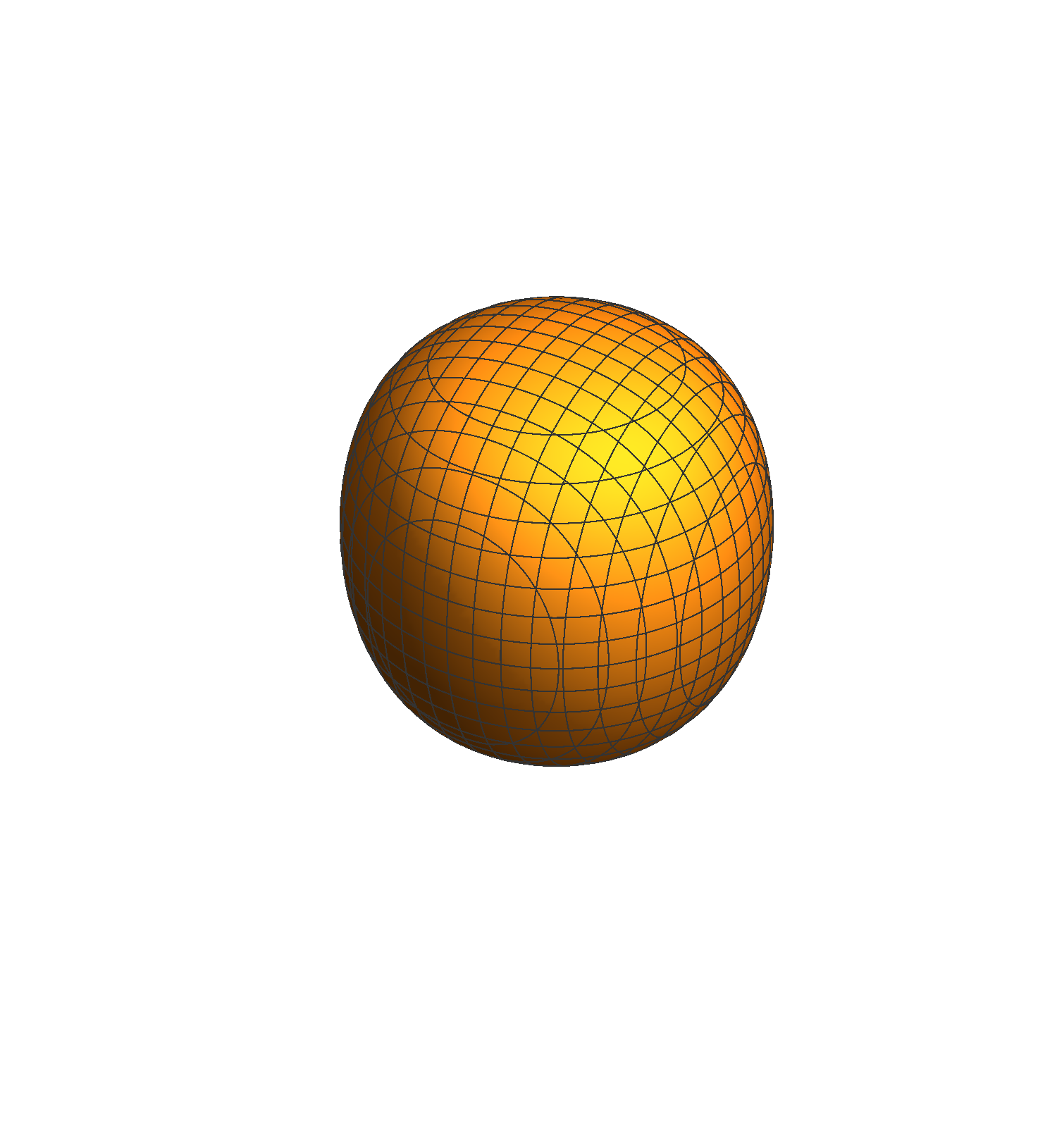
Refer to caption
Figure 3: |ψ1,0,1|2{\lvert\psi_{\mathchoice{\raisebox{-1.5086pt}{\resizebox{1395941}{327680}{\hbox{\raisebox{1.3611pt}{$\displaystyle 1,0,1$}}}}}{\raisebox{-1.5086pt}{\resizebox{1395941}{327680}{\hbox{\raisebox{1.3611pt}{$\textstyle 1,0,1$}}}}}{\raisebox{-1.5086pt}{\resizebox{1328629}{327680}{\hbox{\raisebox{0.95277pt}{$\scriptstyle 1,0,1$}}}}}{\raisebox{-1.50859pt}{\resizebox{1442004}{327680}{\hbox{\raisebox{0.68054pt}{$\scriptscriptstyle 1,0,1$}}}}}}\rvert}^{2}
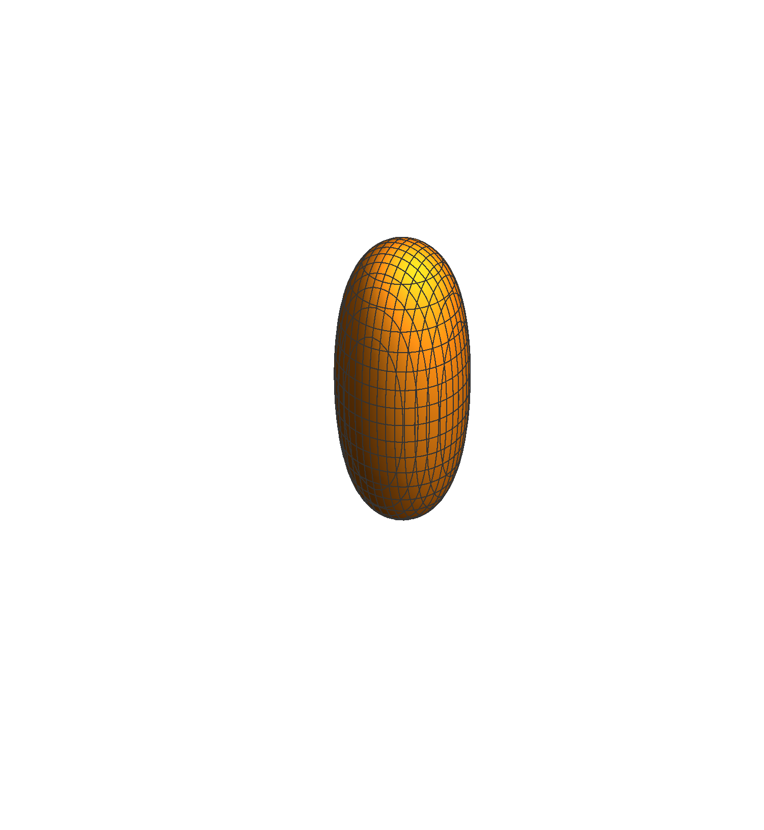
Refer to caption
Figure 4: |ψ2,0,1|2{\lvert\psi_{\mathchoice{\raisebox{-1.5086pt}{\resizebox{1395941}{327680}{\hbox{\raisebox{1.3611pt}{$\displaystyle 2,0,1$}}}}}{\raisebox{-1.5086pt}{\resizebox{1395941}{327680}{\hbox{\raisebox{1.3611pt}{$\textstyle 2,0,1$}}}}}{\raisebox{-1.5086pt}{\resizebox{1328629}{327680}{\hbox{\raisebox{0.95277pt}{$\scriptstyle 2,0,1$}}}}}{\raisebox{-1.50859pt}{\resizebox{1442004}{327680}{\hbox{\raisebox{0.68054pt}{$\scriptscriptstyle 2,0,1$}}}}}}\rvert}^{2}
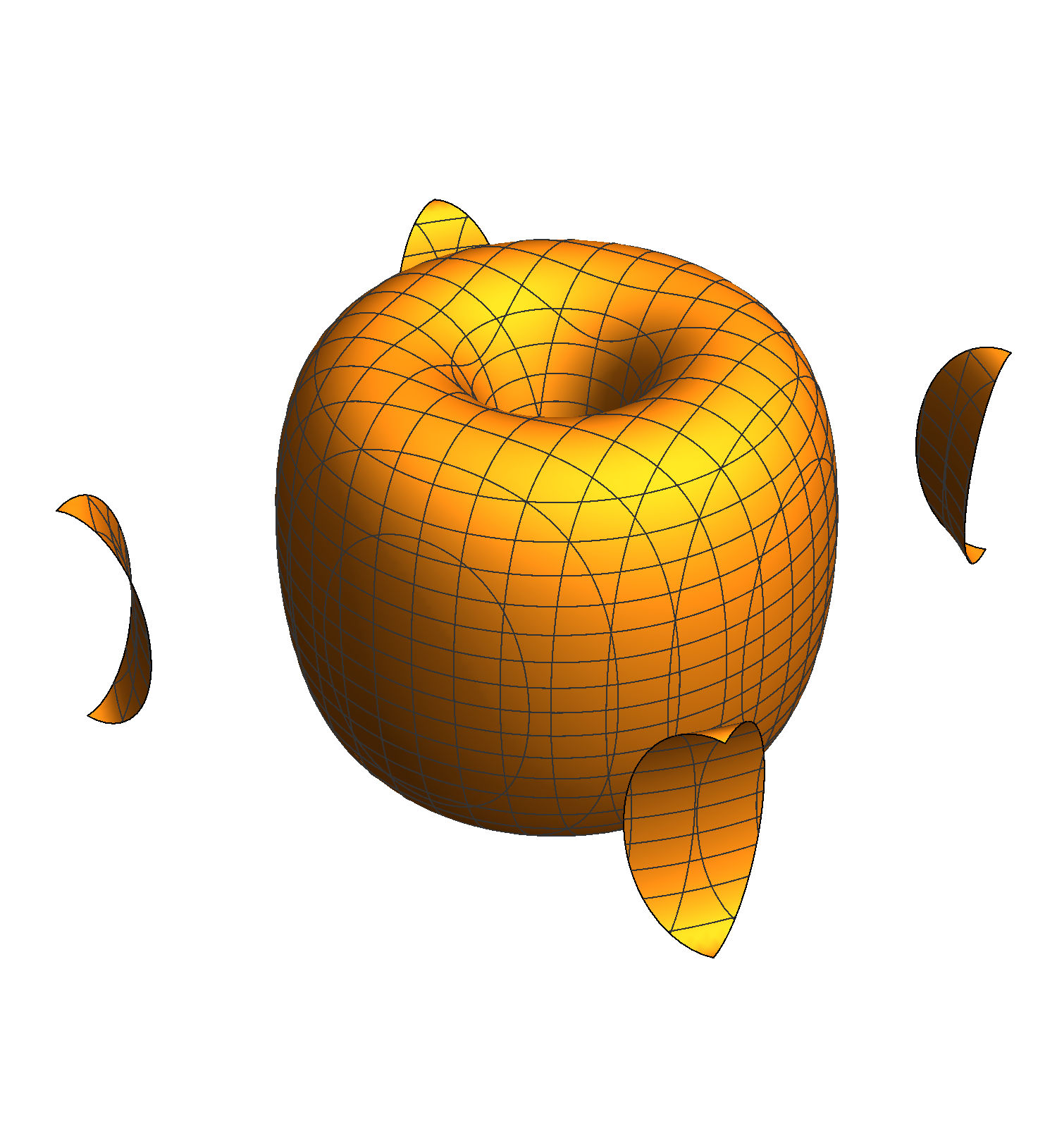
Refer to caption
Figure 5: |ψ1,1,1|2{\lvert\psi_{\mathchoice{\raisebox{-1.5086pt}{\resizebox{1395941}{327680}{\hbox{\raisebox{1.3611pt}{$\displaystyle 1,1,1$}}}}}{\raisebox{-1.5086pt}{\resizebox{1395941}{327680}{\hbox{\raisebox{1.3611pt}{$\textstyle 1,1,1$}}}}}{\raisebox{-1.5086pt}{\resizebox{1328629}{327680}{\hbox{\raisebox{0.95277pt}{$\scriptstyle 1,1,1$}}}}}{\raisebox{-1.50859pt}{\resizebox{1442004}{327680}{\hbox{\raisebox{0.68054pt}{$\scriptscriptstyle 1,1,1$}}}}}}\rvert}^{2}
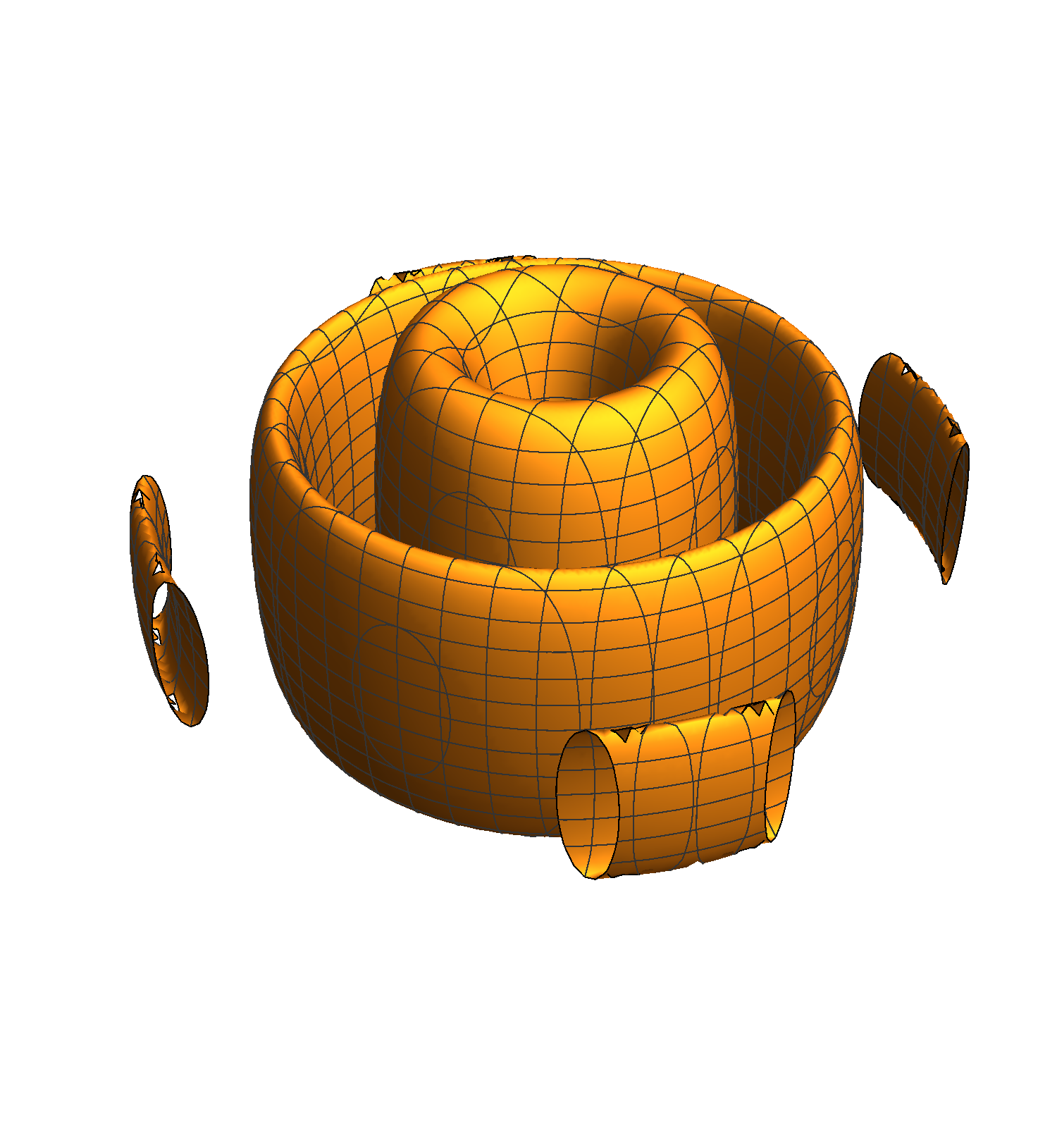
Refer to caption
Figure 6: |ψ2,2,2|2{\lvert\psi_{\mathchoice{\raisebox{-1.5086pt}{\resizebox{1395941}{327680}{\hbox{\raisebox{1.3611pt}{$\displaystyle 2,2,2$}}}}}{\raisebox{-1.5086pt}{\resizebox{1395941}{327680}{\hbox{\raisebox{1.3611pt}{$\textstyle 2,2,2$}}}}}{\raisebox{-1.5086pt}{\resizebox{1328629}{327680}{\hbox{\raisebox{0.95277pt}{$\scriptstyle 2,2,2$}}}}}{\raisebox{-1.50859pt}{\resizebox{1442004}{327680}{\hbox{\raisebox{0.68054pt}{$\scriptscriptstyle 2,2,2$}}}}}}\rvert}^{2}

Comments

In 4.2 we don’t have that extra quantum number pp, as we had in equation (3.6.16). This is obvious as probability density =ψ​ψ∗=\psi\psi^{*}.

In fig. 5 and fig. 6, we have zero probability density on the z-axis. This is evident from the term in (3.6.16):

Jnϕ​[(jnϕ,nr)​ra]J_{\mathchoice{\raisebox{-3.23962pt}{\resizebox{909244}{327680}{\hbox{\raisebox{1.95277pt}{$\displaystyle n_{\phi}$}}}}}{\raisebox{-3.23962pt}{\resizebox{909244}{327680}{\hbox{\raisebox{1.95277pt}{$\textstyle n_{\phi}$}}}}}{\raisebox{-3.37323pt}{\resizebox{858385}{327680}{\hbox{\raisebox{1.42331pt}{$\scriptstyle n_{\phi}$}}}}}{\raisebox{-6.32251pt}{\resizebox{1019006}{327680}{\hbox{\raisebox{1.90553pt}{$\scriptscriptstyle n_{\phi}$}}}}}}\left[\frac{(j_{\mathchoice{\raisebox{-3.23962pt}{\resizebox{2150839}{327680}{\hbox{\raisebox{1.95277pt}{$\displaystyle n_{\phi},n_{r}$}}}}}{\raisebox{-3.23962pt}{\resizebox{2150839}{327680}{\hbox{\raisebox{1.95277pt}{$\textstyle n_{\phi},n_{r}$}}}}}{\raisebox{-3.37323pt}{\resizebox{2076756}{327680}{\hbox{\raisebox{1.42331pt}{$\scriptstyle n_{\phi},n_{r}$}}}}}{\raisebox{-6.32251pt}{\resizebox{2457425}{327680}{\hbox{\raisebox{1.90553pt}{$\scriptscriptstyle n_{\phi},n_{r}$}}}}}})r}{a}\right]

On the z-axis, r=0r=0. So the term becomes

Jnϕ​(0)J_{\mathchoice{\raisebox{-3.23962pt}{\resizebox{909244}{327680}{\hbox{\raisebox{1.95277pt}{$\displaystyle n_{\phi}$}}}}}{\raisebox{-3.23962pt}{\resizebox{909244}{327680}{\hbox{\raisebox{1.95277pt}{$\textstyle n_{\phi}$}}}}}{\raisebox{-3.37323pt}{\resizebox{858385}{327680}{\hbox{\raisebox{1.42331pt}{$\scriptstyle n_{\phi}$}}}}}{\raisebox{-6.32251pt}{\resizebox{1019006}{327680}{\hbox{\raisebox{1.90553pt}{$\scriptscriptstyle n_{\phi}$}}}}}}\left(0\right)

But

Jn​(0)=0​ if ​n≠0J_{n}\left(0\right)=0\text{ if }n\neq 0
Jn​(0)=1​ if ​n=0J_{n}\left(0\right)=1\text{ if }n=0

That is how plots in fig. 5 and fig. 6 differ from plots in fig. 3 and fig. 4. These observations can also, be verified with the radial wavefunction plots (4.1).
In fig. 6, however, we have an additional place (apart from the z-axis) where probability density is vanishing. This can be verified with radial wavefunction plot Rnr,nϕ=R2,2R_{\mathchoice{\raisebox{-3.23962pt}{\resizebox{2150839}{327680}{\hbox{\raisebox{1.95277pt}{$\displaystyle n_{r},n_{\phi}$}}}}}{\raisebox{-3.23962pt}{\resizebox{2150839}{327680}{\hbox{\raisebox{1.95277pt}{$\textstyle n_{r},n_{\phi}$}}}}}{\raisebox{-3.37323pt}{\resizebox{2076756}{327680}{\hbox{\raisebox{1.42331pt}{$\scriptstyle n_{r},n_{\phi}$}}}}}{\raisebox{-6.32251pt}{\resizebox{2457425}{327680}{\hbox{\raisebox{1.90553pt}{$\scriptscriptstyle n_{r},n_{\phi}$}}}}}}=R_{\mathchoice{\raisebox{-1.5086pt}{\resizebox{842744}{327680}{\hbox{\raisebox{1.3611pt}{$\displaystyle 2,2$}}}}}{\raisebox{-1.5086pt}{\resizebox{842744}{327680}{\hbox{\raisebox{1.3611pt}{$\textstyle 2,2$}}}}}{\raisebox{-1.5086pt}{\resizebox{791432}{327680}{\hbox{\raisebox{0.95277pt}{$\scriptstyle 2,2$}}}}}{\raisebox{-1.50859pt}{\resizebox{848119}{327680}{\hbox{\raisebox{0.68054pt}{$\scriptscriptstyle 2,2$}}}}}} in (4.1).

5 Conclusions

We can see from energy eigenvalues expression, equation 3.5.3, that the energy of a free particle in an infinite cylindrical well depends on three quantum numbers associated with three independent directions. But the eigenfunctions, given by equation 3.6.16, depend on an extra quantum number pp. For each nϕn_{\phi}, there are two values of pp. Thus all excited states are 2-fold degenerate.

References