Self-Point-Flow: Self-Supervised Scene Flow Estimation from Point Clouds with Optimal Transport and Random Walk

Ruibo Li^1,2 Guosheng Lin^1,2 Thanks: Corresponding author: G. Lin. (e-mail: $gslin@ntu.edu.sg$ ) Lihua Xie³
¹S-Lab Nanyang Technological University Singapore
²School of Computer Science and Engineering Nanyang Technological University Singapore
³School of Electrical and Electronic Engineering Nanyang Technological University Singapore
E-mail:

\tt ruibo001@e.ntu.edu.sg

\tt\{gslin,elhxie\}@ntu.edu.sg

Abstract

Due to the scarcity of annotated scene flow data, self-supervised scene flow learning in point clouds has attracted increasing attention. In the self-supervised manner, establishing correspondences between two point clouds to approximate scene flow is an effective approach. Previous methods often obtain correspondences by applying point-wise matching that only takes the distance on 3D point coordinates into account, introducing two critical issues: (1) it overlooks other discriminative measures, such as color and surface normal, which often bring fruitful clues for accurate matching; and (2) it often generates sub-par performance, as the matching is operated in an unconstrained situation, where multiple points can be ended up with the same corresponding point. To address the issues, we formulate this matching task as an optimal transport problem. The output optimal assignment matrix can be utilized to guide the generation of pseudo ground truth. In this optimal transport, we design the transport cost by considering multiple descriptors and encourage one-to-one matching by mass equality constraints. Also, constructing a graph on the points, a random walk module is introduced to encourage the local consistency of the pseudo labels. Comprehensive experiments on FlyingThings3D and KITTI show that our method achieves state-of-the-art performance among self-supervised learning methods. Our self-supervised method even performs on par with some supervised learning approaches, although we do not need any ground truth flow for training.

1 Introduction

Scene flow estimation aims to obtain a 3D vector field of points in dynamic scenes, and describes the motion state of each point. Recently, with the popularity of 3D sensors and the great success of deep learning in 3D point cloud tasks, directly estimating the scene flow from point clouds by deep neural networks (DNNs) is an active research topic. DNNs are data-driven, and the supervised training of DNNs requires a large amount of training data with ground truth labels. However, for the scene flow estimation task, no sensor can capture optical flow ground truth in complex environments [19], which makes real-world scene flow ground truth hard to obtain. Due to the scarcity of the ground truth data, recent deep learning based point cloud scene flow estimation methods [14, 7, 38, 23] turn to synthetic data, $e.g.$ the FlyingThings3D dataset [18], for supervised training. However, the domain gap between synthetic data and realistic data is much likely to make the trained models perform poorly in real-world scenes.

Refer to caption — Figure 1: Pseudo ground truth between two point clouds produced by different methods. The green line represents the correct pseudo ground truth whose relative error is less than 10%. The red line represents the wrong pseudo ground truth. (a) pseudo ground truth produced by nearest neighbor search with only 3D point coordinate as measure; (b) pseudo ground truth produced by our optimal transport module; (c) pseudo ground truth produced by our optimal transport module and then refined by our random walk module; (d) ground truth.

To circumvent the dependence on expensive ground truth data, we target self-supervised scene flow estimation from point clouds. Mittal et al. [21] and Wu et al. [38] make the first attempt. These methods search for the closest point in the other point cloud as the corresponding point and use the coordinate difference between each correspondence to approximate the ground truth scene flow. Although achieving promising performance, two issues exist in these methods: (1) searching for correspondences relies only on 3D point coordinates but ignores other measures, such as color and surface normal, which often bring fruitful clues for accurate matching; and (2) the unconstrained search may lead to a degenerated solution, where multiple points match with the same point in the other point cloud, $i.e.$ a many-to-one problem. An example of nearest neighbor search is shown in Fig. 1(a).

In this paper, we assume that an object’s geometric structure and appearance remain unchanged as it moves and the correct corresponding points could be found in its neighborhood. Thus, when searching for point correspondences, we adopt 3D point coordinate, surface normal, and color as measures and encourage each point to be matched with a unique one in the next frame, $i.e.$ one-to-one matching. Naturally, the searching problem can be formulated as an optimal transportation [22], where the transport cost is defined on the three measures, the mass equality constraints are built to encourage one-to-one matching, and the produced optimal assignment matrix indicates the optimal correspondences between the two point clouds. Removing some invalid correspondences with far distance, the coordinate differences between valid correspondences can be treated as the pseudo ground truth flow vectors for training.

Neighboring points in an object often share a similar movement pattern. However, the optimal transport module generates pseudo labels by point-wise matching without considering the local relations among neighboring points, resulting in conflicting pseudo labels in each local region, as shown in Fig. 1(b). To address this issue, we introduce a random walk module to refine the pseudo labels by encouraging local consistency. Viewing each point as a node, we build a graph on the point cloud to propagate and smooth pseudo labels. Specifically, we apply the random walk algorithm [16] in the graph. Using distance on 3D point coordinates as a measure, we build an affinity matrix to describe the similarity between two nodes. In the affinity matrix, closer nodes will be assigned a higher score to ensure local consistency. Normalizing the affinity matrix, we acquire the random walk transition matrix to guide the propagation among the nodes. Through the propagation on the graph, we obtain locally consistent pseudo scene flow labels for scene flow learning.

Our main contributions can be summarized as follows:

•

We propose a novel self-supervised scene flow learning method in point clouds (Self-Point-Flow) to generate pseudo labels by point matching and perform pseudo label refinement by encouraging the local consistency of the pseudo labels;
•

Converting the pseudo label generation problem into a point matching task, we propose an optimal transport module for pseudo label generation by considering multiple clues (3D coordinates, colors and surface normals) and explicitly encouraging one-to-one matching;
•

Neighboring points in an object often share a similar movement pattern. Building a graph on the point cloud, we propose a random walk module to refine the pseudo labels by encouraging local consistency.
•

Our proposed Self-Point-Flow achieves state-of-the-art performance among self-supervised learning methods. Our self-supervised method even performs on par with some supervised learning approaches, although we do not need any ground truth flow for training.

2 Related Work

Supervised scene flow from point clouds Scene flow is first proposed in [31] to represent the 3D motion of points in a scene. Many works [5, 29, 19, 17, 24, 8, 30, 33, 34, 35] have been proposed to recover scene flow from multiple types of data. Recently, directly estimating scene flow from point cloud data using deep learning has become a new research direction. Some approaches [38, 23, 7, 14, 1, 36] learn scene flow in point clouds in a fully supervised manner. Puy et al. [23] first introduce the optimal transport into this field. Added into DNNs, this optimal transport module uses learned features to regress scene flow under full supervision. Different from [23], we focus on unsupervised learning, and our optimal transport module leverages low-level clues to match points for pseudo label generation.

Unsupervised scene flow from point clouds To circumvent the need for expensive ground truth, some approaches [38, 21] target self-supervised learning. Mittal et al. [21] introduce a nearest neighbor loss and an anchored cycle loss. Wu et al. [38] use the Chamfer distance [6] as the main proxy loss. For both the nearest neighbor loss and the Chamfer distance, the nearest neighbor in the other point cloud is regarded as the corresponding point to provide supervision signals. Unlike [21, 38], when building correspondences, we utilize multiple descriptors as clues and leverage global mass constraints to explicitly encourage one-to-one matching in optimal transport.

Unsupervised optical/scene flow from images Other relative topics are unsupervised optical flow from images [25, 39, 42, 13, 12] and unsupervised scene flow from images [9, 11, 37]. In these scopes, the photometric consistency is widely used as a proxy loss to train flow estimation networks by penalizing the photometric differences. Different from these works that directly use the differences as the supervision signal, our method produces pseudo ground truth, which enables our self-supervised method to cooperate with any point-wise loss function.

Optimal transport Optimal transport has been studied in various fields, such as few-shot learning [41, 40], pose estimation [26], semantic correspondence [15], and etc. Most of them embed the optimal transport into DNNs to find correspondences with learnable features. In this paper, we apply optimal transport to self-supervised scene flow learning.

Random walk Random walk is a widely known graphical model [16], which has been used in image segmentation [2] and person re-ID [27]. Bertasius et al. [2] use pixel-to-pixel relations to regularize the pixel prediction results. Shen et al. [27] use inter-image relations to improve image affinity ranking. In this paper, based on the local consistency assumption, we focus on leveraging point-to-point relations for pseudo label smoothness and generation.

3 Method

In this section, we first introduce the theory of optimal transport, and then we discuss the relationship between scene flow labels and point correspondences. Based on the relationship, we solve the pseudo label generation problem by finding point correspondences in an optimal transport framework. Finally, we introduce the details of our proposed pseudo label refinement module that produces dense and locally consistent pseudo labels by the random walk theory. The overview of our method is illustrated in Fig. 2.

3.1 Optimal Transport Revisited

Optimal transport problem [32] seeks a transport plan that moves a source distribution $\mu_{s}$ to a target distribution $\mu_{t}$ with a minimum transport cost. In the discrete versions of this problem, $\mu_{s}$ and $\mu_{t}$ are defined as discrete empirical distributions in $\mathbb{R}^{n}$ . Adapting Kantorovich’s formulation [10] to the discrete setting, the space of transport plans is a polytope, and the discrete optimal transport problem can be written as:

		$\displaystyle{\displaystyle\bm{U}}^{*}=\mathop{\arg\min}_{\bm{U}\in\mathbb{R}^{n\times n}_{+}}\sum_{ij}{\bm{H}}_{ij}{\bm{U}}_{ij}$		(1)
		$\displaystyle\text{s.t.}\quad{\bm{U}}{\bm{1}}_{n}=\mu_{s},\ {\bm{U}}^{\mathsf{T}}{\bm{1}}_{n}=\mu_{t},$		(1)

where $\bm{H}_{ij}\geq 0$ is the transport cost from sample $i$ to sample $j$ , $\bm{U}^{*}$ is the optimal assignment matrix and each element $\bm{U}_{ij}^{*}$ describes the optimal amount of mass transported from sample $i$ to sample $j$ .

3.2 Pseudo Label Generation by OT

Given two consecutive point clouds, ${\bm{P}}=\{{\bm{p}}_{i}\in\mathbb{R}^{3}\}_{i=1}^{n}$ at frame $t$ and ${\bm{Q}}=\{{\bm{q}}_{i}\in\mathbb{R}^{3}\}_{j=1}^{n}$ at frame $t+1$ , the task of point cloud scene flow estimation aims to predict the scene flow ${\bm{F}}=\{{\bm{f}}_{i}\in\mathbb{R}^{3}\}_{i=1}^{n}$ for point cloud $\bm{P}$ , where each element $\bm{f}_{i}$ represents the translation of point $\bm{p}_{i}$ from frame $t$ to frame $t+1$ .

Unlike fully supervised scene flow learning, where scene flow labels are available, the self-supervised scene flow learning should produce pseudo labels or design self-supervised losses for training. In this paper, we study how to generate effective pseudo labels for scene flow learning.

Extracting pseudo labels via point matching Scene flow describes the motion between two consecutive point clouds. Ideally, if no viewpoint shift and occlusions exist, following the ground truth scene flow labels $\bm{D}$ , the first point cloud $\bm{P}$ can be projected into the next frame and fully occupy the second point cloud $\bm{Q}$ :

{\bm{P}}+{\bm{D}}={\bm{\pi}}\ {\bm{Q}},

(2)

where ${\bm{\pi}}\in\{0,1\}^{n\times n}$ is a permutation matrix to indicate the point correspondences between the two point clouds. Therefore, for a pair of consecutive point clouds $\bm{P}$ and $\bm{Q}$ , if we can accurately match points in the two point clouds, $i.e.$ accurately computing the permutation matrix $\bm{\pi}$ , the correspondences derived from $\bm{\pi}$ can help us recover the ground truth scene flow labels $\bm{D}$ . In other words, we can solve the pseudo label generation problem by finding point correspondences.

When building correspondences, a straightforward way is to directly match the points from $\bm{P}$ to $\bm{Q}$ . However, for the self-supervised scene flow estimation task, given predicted scene flow $\bm{F}$ , we propose a pre-warping operation to warp the first point cloud $\bm{P}$ by the predicted scene flow $\bm{F}$ , and then find correspondences by matching points from the pre-warped first point cloud, denoted as $\bm{\hat{P}}$ , to the second point cloud $\bm{Q}$ . Although the predicted scene flow is inaccurate at the beginning of the training, the predictions will be gradually improved as the training continues, which makes the matching from $\bm{\hat{P}}$ to $\bm{Q}$ easier than the matching from $\bm{P}$ to $\bm{Q}$ . In Sec. 4.3, we show that the matching from $\bm{\hat{P}}$ to $\bm{Q}$ can make our self-supervised method achieve better performance.

Building optimal transport problem Using 3D point coordinate, color, and surface normal as measures to compute the matching cost and formulating one-to-one matching as the mass equality constraints, we build an optimal transport problem from $\bm{\hat{P}}$ to $\bm{Q}$ ,

		$\displaystyle\bm{T}^{*}=\mathop{\arg\min}_{\bm{T}\in\mathbb{R}^{n\times n}_{+}}\sum_{ij}{\bm{C}}_{ij}\bm{T}_{ij}$		(3)
		$\displaystyle\text{s.t.}\quad\bm{T}{\bm{1}}_{n}={\bm{\mu}_{\hat{p}}},\ \bm{T}^{\mathsf{T}}{\bm{1}}_{n}={\bm{\mu}_{q}}.$		(3)

$\bm{T}^{*}$ is the optimal assignment matrix from $\bm{\hat{P}}$ to $\bm{Q}$ . $\bm{C}_{ij}$ is the transport cost from the $i$ -th point in $\bm{\hat{P}}$ to the $j$ -th point in $\bm{Q}$ . The transport cost $\bm{C}_{ij}$ is obtained by computing the pairwise difference between $\bm{\hat{p}_{i}}$ and $\bm{q_{j}}$ in the three measures. The coordinate cost $\bm{C}_{ij}^{d}$ and the color cost $\bm{C}_{ij}^{c}$ are defined on a Gaussian function:

{\bm{C}}_{ij}^{d}=1-{\rm\exp}(-\frac{\|\bm{\hat{p}}_{i}-\bm{q}_{j}\|^{2}}{2\theta_{d}^{2}}),

(4)

{\bm{C}}_{ij}^{c}=1-{\rm\exp}(-\frac{\|\bm{k}_{{\hat{p}},i}^{c}-\bm{k}_{q,j}^{c}\|^{2}}{2\theta_{c}^{2}}),

(5)

where $\|\cdot\|$ denotes the $L^{2}$ norm of a vector, $\theta_{d}$ and $\theta_{c}$ are user defined parameters, $\bm{\hat{p}}_{i}$ and $\bm{q}_{j}$ represent the coordinates of the $i$ -th point and the $j$ -th point, $\bm{k}_{{\hat{p}},i}^{c}$ and $\bm{k}_{q,j}^{c}$ are the colors of the two points. The surface normal cost is calculated using the cosine similarity:

{\bm{C}}_{ij}^{s}=1-\frac{\|(\bm{k}_{{\hat{p}},i}^{s})^{\mathsf{T}}\bm{k}_{{q},j}^{s}\|}{\|\bm{k}_{{\hat{p}},i}^{s}\|\cdot\|\bm{k}_{{q},j}^{s}\|},

(6)

where $\bm{k}_{{\hat{p}},i}^{s}$ and $\bm{k}_{q,j}^{s}$ are the surface normals of the two points. The final transport cost is the sum of the three individual costs:

{\bm{C}}_{ij}={\bm{C}}_{ij}^{d}+{\bm{C}}_{ij}^{c}+{\bm{C}}_{ij}^{s}.

(7)

In order to encourage one-to-one matching, in the equality constraints of Eq. 3, we set ${\bm{\mu}_{\hat{p}}}=\frac{1}{n}{\bm{1}}_{n}$ and ${\bm{\mu}_{q}}=\frac{1}{n}{\bm{1}}_{n}$ . In this case, the row sum and the column sum of assignment matrix $\bm{T}$ are constrained to be a uniform distribution, which will alleviate the many-to-one matching problem.

Efficiently solving with the Sinkhorn algorithm To efficiently solve the optimal transport problem, we smooth the above problem with an entropic regularization term:

		$\displaystyle\bm{T}^{*}=\mathop{\arg\min}_{\bm{T}\in\mathbb{R}^{n\times n}_{+}}\sum_{ij}{\bm{C}}_{ij}\bm{T}_{ij}+\varepsilon\bm{T}_{ij}(\log{\bm{T}_{ij}}-1)$		(8)
		$\displaystyle\text{s.t.}\quad\bm{T}{\bm{1}}_{n}={\bm{\mu}_{\hat{p}}},\ \bm{T}^{\mathsf{T}}{\bm{1}}_{n}={\bm{\mu}_{q}}.$		(8)

$\varepsilon$ is the regularization parameter. The Sinkhorn algorithm [4] can be employed to solve this entropy-regularized formulation. The details are presented in Algorithm 1.

Algorithm 1 Optimal transport

Input: Transport cost matrix $\bm{C}$ ; hyperparameter $\varepsilon$ , iteration number $L_{o}$ ;
Output: Optimal transport matrix ${T}^{*}$ ;
Procedure:

{\bm{K}}\leftarrow{\rm\exp}(-{\bm{C}}/\varepsilon)

;

{\bm{\mu}_{\hat{p}}}\leftarrow\frac{1}{n}{\bm{1}}_{n}

{\bm{\mu}_{q}}\leftarrow\frac{1}{n}{\bm{1}}_{n}

{\bm{a}}\leftarrow\frac{1}{n}{\bm{1}}_{n}

;

3: for

l=1,...,L_{o}

{\bm{b}}\leftarrow{\bm{\mu}_{q}}/({\bm{K}}^{\mathsf{T}}{\bm{a}})

;

{\bm{a}}\leftarrow{\bm{\mu}_{\hat{p}}}/({\bm{K}}{\bm{b}})

;

6: end for

{T}^{*}\leftarrow\operatorname{diag}(\bm{a}){\bm{K}}\operatorname{diag}(\bm{b})

Selecting hard correspondences and generating pseudo labels from assignment matrix The optimal transport plan $\bm{T}^{*}$ derived from Algorithm 1 is a soft assignment matrix, where $\bm{T}^{*}_{ij}\in[0,1]$ . To obtain hard correspondences from $\bm{\hat{P}}$ to $\bm{Q}$ , in each row of $\bm{T}^{*}$ , we set the element with the maximum value to 1 and the remaining elements to 0 so that the point with the highest transport score is selected as the unique corresponding point in this row. The produced hard assignment matrix is donated as $\bm{T}^{*}_{\pi}$ . According to the Eq. 2, we have the pseudo scene flow labels $\bm{\tilde{D}}$ :

{\bm{\tilde{D}}}={\bm{T}^{*}_{\pi}}{\bm{Q}}-{\bm{P}}.

(9)

Removing some invalid pseudo scene flow labels with too large displacements (larger than 3.5 $m$ ), we obtain a set of valid pseudo labels $\bm{\tilde{D}}_{M}$ for the valid labeled points $\bm{P}_{M}$ . And the remaining points without valid pseudo labels are denoted as $\bm{P}_{S}$ .

3.3 Pseudo Label Refinement by Random Walk

The optimal transport module generates pseudo labels by point-wise matching but lacks in capturing the local relations among neighboring points, resulting in conflicting pseudo labels in each local region. Moreover, after the pseudo label generation module, there are still some points without valid pseudo labels. To address the issues, we propose a pseudo label refinement module to encourage the local consistency of pseudo labels and infer new pseudo labels for those unlabeled points.

Building graph on the point cloud Viewing each point as a node, we build a graph $G(V,E)$ on the first point cloud $\bm{P}$ , shown in Fig. 3. According to the labeling state of each point, the nodes are separated into two sets, the labeled nodes associated with $\bm{P}_{M}$ and the unlabeled nodes associated with $\bm{P}_{S}$ . $V_{m}=\{1,2,...,n_{m}\}$ and $V_{s}=\{1,2,...,n_{s}\}$ represent the labeled node set and the unlabeled node set, respectively. $n_{m}$ and $n_{s}$ are the number of nodes in the two sets. Subsequently, the entire graph $G(V,E)$ can be divided into two suggraphs: 1) a fully-connected undirected subgraph $G_{1}(V_{m},E_{m})$ on labeled nodes $V_{m}$ to smooth the pseudo labels of the labeled points; 2) a directed subgraph $G_{2}(V,E_{s})$ from labeled nodes $V_{m}$ to unlabeled nodes $V_{s}$ to generate new pseudo labels for the unlabeled points. In this procedure, the pseudo labels of the unlabeled points are entirely dependent on those of the labeled points. Therefore, we can first propagate pseudo labels on the undirected subgraph and then on the directed subgraph. The propagation operation can be achieved by the random walk algorithm [16].

Figure 3: Illustration of the graph

G

. This graph consists of two subgraphs: a fully-connected undirected subgraph for pseudo label smoothing on labeled points and a directed subgraph for new pseudo label generation on unlabeled points.

Propagating on the undirected subgraph The fully-connected undirected subgraph is constructed to improve the local consistency of pseudo labels for the labeled point set $\bm{P}_{M}$ . The random walk operation on this subgraph can be modeled with a $n_{m}\times n_{m}$ transition matrix $\bm{A}^{1}$ . $\bm{A}^{1}_{ij}~\in~[0,1]$ denotes the transition probability between $i$ -th and $j$ -th nodes with constraints $\sum_{j}\bm{A}^{1}_{ij}=1$ for all $j$ .

To encourage the local consistency, we use the nearness among nodes as the measure to build the transition matrix so that the closer nodes will be assigned a higher transition probability. Firstly, we denote a symmetric $n_{m}\times n_{m}$ affinity matrix $\bm{W}^{1}$ , where each element $\bm{W}^{1}_{ij}$ describes how near the nodes $i$ and $j$ are,

{\bm{W}}_{ij}^{1}={\rm\exp}(-\frac{\|\bm{p}_{i}-\bm{p}_{j}\|^{2}}{2\theta_{r}^{2}}),

(10)

where $\theta_{r}$ is a hyperparameter, $\bm{p}_{i}$ and $\bm{p}_{j}$ are point coordinates associated with nodes $i$ and $j$ . Then, we normalize the affinity matrix $\bm{W}^{1}$ to obtain the transition matrix $\bm{A}^{1}$ , where each element $\bm{A}_{ij}^{1}$ is written as:

{\bm{A}}_{ij}^{1}=\frac{{\bm{W}}_{ij}^{1}}{\sum_{j\neq i}{\bm{W}}_{ij}^{1}}.

(11)

The $t$ -th iteration of random walk refinements on the pseudo labels can be expressed as

{\bm{\tilde{D}}_{M}^{(t)}}=\alpha{\bm{A}^{1}}{\bm{\tilde{D}}_{M}^{(t-1)}}+(1-\alpha){\bm{\tilde{D}}_{M}^{(0)}},

(12)

where ${\bm{\tilde{D}}}_{M}^{(0)}$ are the initial pseudo labels derived from the pseudo label generation module, ${\bm{\tilde{D}}}_{M}^{(t-1)}$ are the refined labels after $t-1$ random walk steps, and $\alpha$ is a parameter $[0,1]$ to control the tradeoff between the random walk refinements and the initial values.

When applying the random walk procedure until convergence, $i.e.$ $t=\infty$ , according to [2, 27], the final random walk refinements can be written as

{\bm{\tilde{D}}_{M}^{(\infty)}}=(1-\alpha)({\bm{I}}-\alpha{\bm{A}^{1}})^{-1}{\bm{\tilde{D}}_{M}^{(0)}},

(13)

where ${\bm{I}}$ is the identity matrix. After $L_{r}$ random walk steps, we treat the produced random walk refinements as the refined pseudo labels of the labeled points, ${\bm{\widehat{D}}}_{M}=\bm{\tilde{D}}_{M}^{(L_{r})}$ .

Propagating on the directed subgraph The undirected subgraph is built to infer new pseudo labels for the unlabeled point set $\bm{P}_{S}$ based on the refined pseudo labels of the labeled point set, ${\bm{\widehat{D}}}_{M}$ . Similar to the propagation process on the undirected subgraph, we first define a $n_{s}\times n_{m}$ affinity matrix $\bm{W}^{2}$ to describe the nearness between each point in $\bm{P}_{S}$ and each point in $\bm{P}_{S}$ . Then we obtain a $n_{s}\times n_{m}$ transition matrix $\bm{A}^{2}$ by normalizing the affinity matrix $\bm{W}^{2}$ . The calculation of $\bm{W}^{2}$ and $\bm{A}^{2}$ is the same as that of $\bm{W}^{1}$ and $\bm{A}^{1}$ , shown in Eq. 10 and Eq. 11. Based on the transition matrix $\bm{A}^{2}$ and the refined pseudo labels ${\bm{\widehat{D}}}_{M}$ , we obtain the new pseudo labels ${\bm{\widehat{D}}}_{S}$ for the unlabeled points:

{\bm{\widehat{D}}}_{S}=\bm{A}^{2}{\bm{\widehat{D}}}_{M}.

(14)

Training with pseudo labels Combining the refined pseudo labels ${\bm{\widehat{D}}}_{M}$ and the new pseudo labels ${\bm{\widehat{D}}}_{S}$ , we obtain the final refined pseudo labels $\bm{\widehat{D}}$ for the entire point cloud $\bm{P}$ in self-supervised learning. The training loss in our self-supervised learning method can be computed by:

Loss=f_{loss}({\bm{\widehat{D}}},{\bm{F}}),

(15)

where $f_{loss}$ is any per-point loss function, $\bm{F}$ is the predicted scene flow. Specifically, we set $f_{loss}$ to per-point $L_{2}$ -norm loss function for scene flow learning in this paper.

4 Experiments

We first compare our method with two state-of-the-art self-supervised scene flow estimation methods in Sec. 4.1. Then, we compare our self-supervised models with state-of-the-art fully-supervised models in Sec. 4.2. Finally, we conduct ablation studies to analyze the effectiveness of each component in Sec. 4.3. In this section, we adopt the FlowNet3D [14] as our default scene flow estimation model with only point coordinates as input. Experiments will be conducted on FlyingThings3D [18] and KITTI 2015 [19, 20] datasets. Point clouds are not directly provided in the two original datasets. Following [23], we denote the two processed point cloud datasets provided by [7] as FT3D_s and KITTI_s. And we denote the two processed datasets provided by [14] as FT3D_o and KITTI_o.

Evaluation metrics. We adopt four evaluation metrics used in [14], [7], [23]. Let $\bm{Y}$ denote the predicted scene flow, and $\bm{D}$ be the ground truth scene flow. The evaluate metrics are computed as follows. EPE(m): the main metric, $\|\bm{Y}^{*}-\bm{Y}_{gt}\|_{2}$ average over each point. AS(%): the percentage of points whose EPE $<$ 0.05m or relative error $<5\%$ . AR(%): the percentage of points whose EPE $<$ 0.1m or relative error $<10\%$ . Out(%): the percentage of points whose EPE $>$ 0.3m or relative error $>10\%$ .

4.1 Comparison with self-supervised methods

Comparison with PointPWC-Net [38]. Wu et al. [38] introduce Chamfer distance, smoothness constraint, and Laplacian regularization for self-supervised learning. Following the experimental settings of [38], we first train the FlowNet3D model with our self-supervised method on FT3D_s and then evaluate on FT3D_s and KITTI_s. During training, we use the whole training set in FT3D_s for training. Besides, we also try to add the cycle-consistency regularization [14] into our training loss. The detailed experimental setting could be found in supplementary.

The results are shown in Table 1. Our method outperforms self-supervised PointPWC-Net [38] on all metrics and shows significantly better generalization ability on KITTI, although the network capacity of our used FlowNet3D is worse than that of their PointPWC-Net. Adding the cycle-consistency regularization to the loss function, our model gains a further improvement.

Table 1: Evaluation results on FlyingThings3D and KITTI datasets using the process point cloud data provided by [7]. Full means fully-supervised training, Self means self-supervised training.

\dagger

means that we add a cycle-consistency regularization [14] into the training loss. Without using ground truth flow, our self-supervised method outperforms PointPWC-Net on the two datasets and even performs on par with some supervised approaches.

Dataset	Method	Sup.	EPE $\downarrow$	AS $\uparrow$	AR $\uparrow$	Out $\downarrow$
FT3D_s	PointPWC-Net [38]	Self	0.1213	32.39	67.42	68.78
	Ours	Self	0.1208	36.68	70.22	65.35
	Ours^†	Self	0.1009	42.31	77.47	60.58
	SPLATFlowNet [28]	Full	0.1205	41.97	71.80	61.87
	original BCL [7]	Full	0.1111	42.79	75.51	60.54
	FlowNet3D [14]	Full	0.0864	47.89	83.99	54.64
	HPLFlowNet [7]	Full	0.0804	61.44	85.55	42.87
	PointPWC-Net [38]	Full	0.0588	73.79	92.76	34.24
KITTI_s	PointPWC-Net [38]	Self	0.2549	23.79	49.57	68.63
	Ours	Self	0.1271	45.83	77.77	41.44
	Ours^†	Self	0.1120	52.76	79.36	40.86
	SPLATFlowNet [28]	Full	0.1988	21.74	53.91	65.75
	original BCL [7]	Full	0.1729	25.16	60.11	62.15
	FlowNet3D [14]	Full	0.1064	50.65	80.11	40.03
	HPLFlowNet [7]	Full	0.1169	47.83	77.76	41.03
	PointPWC-Net [38]	Full	0.0694	72.81	88.84	26.48

Comparison with JGF [21]. Mittal et al. [21] propose a nearest neighbor loss and an anchored cycle loss for self-supervised training. In [21], they split the KITTI_o into two sets, 100 pairs of point clouds for training, denoted as KITTI_v, and the remaining 50 pairs for testing, denoted as KITTI_t. Moreover, they also leverage an additional real-world outdoor point cloud dataset, nuScenes [3], to augment their training data. In [21], all networks are initialized with a Flownet3D model [14] pre-trained on FlyingThing3D.

In our experiment, we use the raw data from KITTI to produce point clouds as our training data. Because the point clouds in KITTI_o belong to 29 scenes in KITTI, to avoid the overlap of training data and test data, we produce training point clouds from the remaining 33 scenes. Extracting a pair of point clouds at every five frames, we build a self-supervised training set containing 6,068 pairs, denoted as KITTI_r. For comparison, we test our model on the same KITTI_t with 50 test pairs. In each test pair, our model is evaluated by processing 2,048 random points. The detailed experimental setting is in supplementary.

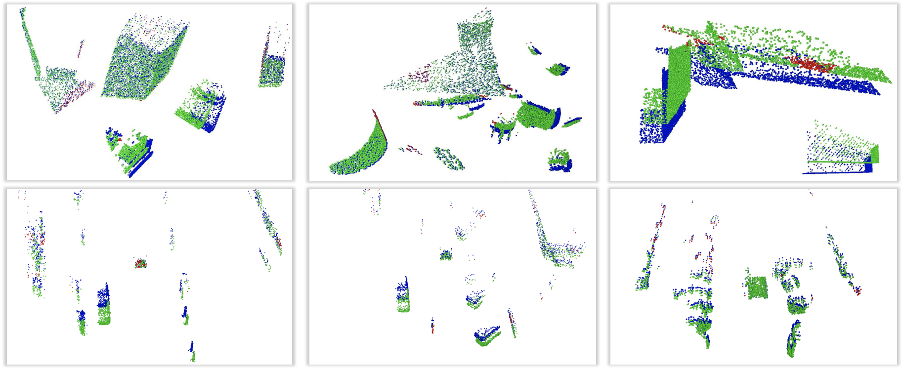
The results are shown in Table 2. Our model trained on KITTI_r outperforms their model by 18.3% in EPE, which is pre-trained on FT3D and then trained on KITTI_v, although training from scratch is much more challenging than fine-tuning a pre-trained model for self-supervised learning. After further fine-tuned on KITTI_v, our model achieves comparable performance to their model, which is pre-trained on FT3D and then trained on nuScenes and KITTI_v. When using the parameters of self-supervised models as initial weights and performing fully-supervised training on KITTI_v, our model outperforms theirs on all metrics. Fig. 5 displays our produced pseudo ground truth for some examples in KITTI_v.

Table 2: Evaluation results on KITTI_t according to the test settings of Mittal et al. [21].

\ddagger

means a fully-supervised fine-tuning on KITTI_v.

Method	Pre-trained	Training data	EPE $\downarrow$	AS $\uparrow$	AR $\uparrow$
[21]	$\checkmark$	FT3D_o + KITTI_v	0.1260	32.00	73.64
[21]	$\checkmark$	FT3D_o + nuScenes + KITTI_v	0.1053	46.48	79.42
Ours		KITTI_r	0.1029	35.68	68.55
Ours		KITTI_r + KITTI_v	0.0895	41.74	75.01
[21]	$\checkmark$	FT3D_o + nuScenes + KITTI_v^‡	0.0912	47.92	79.63
Ours		KITTI_r + KITTI_v^‡	0.0720	50.12	82.38

4.2 Comparison with fully-supervised methods

In Table 1, we compare our self-supervised model with some fully-supervised methods, which are also trained on FT3D_s and tested on FT3D_s and KITTI_s. As shown in Table 1, adding a cycle-consistency regularization, our self-supervised method outperforms SPLATFlowNet [28] on FT3D_s and generalizes better on KITTI_s than SPLATFlowNet [28], original BCL [7], and HPLFlowNet [7], although we do not use any ground truth flow for training. Qualitative results are shown in Fig. 4.

In Table 3, using KITTI_o as test set, we compare our self-supervised model trained on KITTI_r with some fully-supervised methods trained on FT3D_o, following the test procedure of FLOT [23]. Despite using the same scene flow estimation model, our self-supervised FlowNet3D trained on KITTI_r outperforms supervised FlowNet3D [14] trained on FT3D_o by 39.3% in the metric of EPE. It demonstrates that, for the FlowNet3D model, self-supervised learning on KITTI with our method is much more effective than supervised learning on FlyingThings3D in real-world scenes. Furthermore, as shown in Table 3, our self-supervised method has achieved a close performance to the state-of-the-art supervised method, FLOT [23], on KITTI_o dataset. Fig. 4 provides some example results.

Table 3: Evaluation results on KITTI_o. Without using ground truth flow, our self-supervised method outperforms supervised FlowNet3D [14] and achieves comparable performance to the state-of-the-art supervised method, FLOT [23].

Method	Sup.	Training data	EPE $\downarrow$	AS $\uparrow$	AR $\uparrow$	Out $\downarrow$
FlowNet3D [14]	Full	FT3D_o	0.173	27.6	60.9	64.9
FLOT [23]	Full	FT3D_o	0.107	45.1	74.0	46.3
Ours	Self	KITTI_r	0.105	41.7	72.5	50.1

4.3 Ablation studies

In this section, we conduct ablation studies to analyze the effectiveness of each component. All models are trained on KITTI_r and evaluated on KITTI_o.

Ablation study for pseudo label generation module. In this module, for good point matching, we adopt color and surface normal as additional measures to build the transport cost matrix and establish the global constraints to enforce one-to-one marching. To verify the effectiveness of our module, we design a baseline method, named greedy search, which directly finds the point with the lowest transport cost in another point cloud as the corresponding point without any constraints.

Firstly, we analyze the impact of the color measure and the surface normal measure. As shown in Table 4, for both greedy search method and optimal transport method, adding color and surface normal as measures can boost AS by around 10 to 17 points. Compared with the original optimal transport with only 3D point coordinate as a measure, our proposed pseudo label generation module brings a 139% improvement on AS, which demonstrates the discriminative ability of color and surface normal in finding correspondences.

Secondly, we analyze the impact of the global constraints. As shown in Table 4, for all three kinds of measure combinations, adding the global constraints can increase AS by about 5 to 9 points, which means that addressing the many-to-one problem in point matching can greatly improve the quality of produced pseudo labels.

Thirdly, we compare different matching strategies in our module. In our optimal transport, we search for correspondences by matching from the pre-warped first point cloud to the second point cloud, denoted as $\bm{\widehat{P}}~\to~\bm{Q}$ , and regard the point with the highest transport score as the corresponding point, denoted as Hard matching. To evaluate the effectiveness of our matching strategy, as shown in Table 5, we design two baseline methods: 1) baseline1 matches from the first point cloud to the second one, denoted as $\bm{P}~\to~\bm{Q}$ , 2) baseline 2 produces a soft corresponding point by using the transport score as the weight to perform a weighted summation of all candidate points. This process is denoted as Soft matching. As shown in Table 5, our method outperforms baseline1 and baseline2 by about 10 points on AS, which demonstrates the effectiveness of our matching strategy.

Table 4: Ablation study for color measure, surface normal measure and the matching constraints in our pseudo label generation module (PLGM).

Method	Coordinate	Color	Norm	Constraint	AS $\uparrow$
Greedy search (Baseline)	$\checkmark$				1.85
+ Color	$\checkmark$	$\checkmark$			11.25
+ Color + Norm	$\checkmark$	$\checkmark$	$\checkmark$		18.89
Optimal Transport	$\checkmark$			$\checkmark$	10.19
+ Color	$\checkmark$	$\checkmark$		$\checkmark$	21.51
+ (Color + Norm)/Our PLGM	$\checkmark$	$\checkmark$	$\checkmark$	$\checkmark$	24.36

Table 5: Ablation study for different matching strategies in our pseudo label generation module (PLGM).

\bm{P}~\to~\bm{Q}

: match from the first point cloud to the second point cloud.

\bm{\widehat{P}}~\to~\bm{Q}

: match from the pre-warped first point cloud to the second point cloud. Soft matching: produce labels by soft correspondences. Hard matching: produce labels by hard correspondences.

Method	$\bm{P}\to\bm{Q}$	$\bm{\widehat{P}}\to\bm{Q}$	Soft matching	Hard matching	AS $\uparrow$
Baseline1	$\checkmark$			$\checkmark$	12.52
Baseline2		$\checkmark$	$\checkmark$		13.16
Our PLGM		$\checkmark$		$\checkmark$	24.36

Ablation study for pseudo label refinement module. This module employs random walk operations to improve the local consistency of pseudo labels. In this module, we build two subgraphes: an undirected one for label smoothness and a directed one for new label generation in unlabeled points. To verify the effectiveness of our module, we design a naive smoothing unit (NS) that finds neighboring points by KNN search and outputs the average label of the neighboring points as the refined label. As show in Table 6, smoothing labels by random walk operation on the undirected subgraph (UG) improves AS from 24.36 to 40.88. And the improvement from UG is significantly greater than that from the naive smoothing unit (NS). By further generating new labels for the unlabeled points via random walk operation on the directed subgraph (DG), we achieve another improvement on AS by 0.86. The great improvement demonstrates the effectiveness of our pseudo label refinement module. And the impact of different random walk steps on our method is shown in Table 7.

Time consumption of our pseudo-label generation process. To process a scene containing 2,048 points in KITTI_r, the pseudo label generation module takes about 3.2ms and the pseudo label refinement module takes about 75.6ms on a single 2080ti GPU. Thus, the total time consumption for a scene is 78.8ms.

Table 6: Ablation study for our pseudo label refinement module (PLRM). NS: naive smoothing unit. UG: smooth labels by random walk operation on the undirected subgraph. DG: generate new labels by random walk operation on the directed subgraph.

Method	NS	UG	DG	AS $\uparrow$
Our PLGM				24.36
+ NS	$\checkmark$			27.53
+ UG		$\checkmark$		40.88
+ (UG +UG)/Our PLRM		$\checkmark$	$\checkmark$	41.74

Table 7: The impact of the iteration number of the random walk operation on our method.

Iteration number	1	5	10	20	$\infty$
AS $\uparrow$	37.29	38.49	39.71	40.11	41.74

5 Conclusions

In this paper, we propose a novel self-supervised scene flow learning method in point clouds to produce pseudo labels via point matching and perform pseudo label refinement by encouraging the local consistency. Comprehensive experiments show that our method achieves state-of-the-art performance among self-supervised learning methods. Our self-supervised method even performs on par with some supervised learning approaches, although we do not need any ground truth flow for training.

6 Acknowledgements

This research was conducted in collaboration with SenseTime. This work is supported by A*STAR through the Industry Alignment Fund - Industry Collaboration Projects Grant. This work is also supported by the National Research Foundation, Singapore under its AI Singapore Programme (AISG Award No: AISG-RP-2018-003), and the MOE Tier-1 research grants: RG28/18 (S) and RG22/19 (S).

References

[1] Aseem Behl, Despoina Paschalidou, Simon Donné, and Andreas Geiger. Pointflownet: Learning representations for rigid motion estimation from point clouds. In Proceedings of the IEEE Conference on Computer Vision and Pattern Recognition, pages 7962–7971, 2019.
[2] Gedas Bertasius, Lorenzo Torresani, Stella X Yu, and Jianbo Shi. Convolutional random walk networks for semantic image segmentation. In Proceedings of the IEEE Conference on Computer Vision and Pattern Recognition, pages 858–866, 2017.
[3] Holger Caesar, Varun Bankiti, Alex H Lang, Sourabh Vora, Venice Erin Liong, Qiang Xu, Anush Krishnan, Yu Pan, Giancarlo Baldan, and Oscar Beijbom. nuscenes: A multimodal dataset for autonomous driving. In Proceedings of the IEEE/CVF Conference on Computer Vision and Pattern Recognition, pages 11621–11631, 2020.
[4] Marco Cuturi. Sinkhorn distances: Lightspeed computation of optimal transport. In Advances in neural information processing systems, pages 2292–2300, 2013.
[5] Ayush Dewan, Tim Caselitz, Gian Diego Tipaldi, and Wolfram Burgard. Rigid scene flow for 3d lidar scans. In 2016 IEEE/RSJ International Conference on Intelligent Robots and Systems (IROS), pages 1765–1770. IEEE, 2016.
[6] Haoqiang Fan, Hao Su, and Leonidas J Guibas. A point set generation network for 3d object reconstruction from a single image. In Proceedings of the IEEE conference on computer vision and pattern recognition, pages 605–613, 2017.
[7] Xiuye Gu, Yijie Wang, Chongruo Wu, Yong Jae Lee, and Panqu Wang. Hplflownet: Hierarchical permutohedral lattice flownet for scene flow estimation on large-scale point clouds. In Proceedings of the IEEE Conference on Computer Vision and Pattern Recognition, pages 3254–3263, 2019.
[8] Frédéric Huguet and Frédéric Devernay. A variational method for scene flow estimation from stereo sequences. In 2007 IEEE 11th International Conference on Computer Vision, pages 1–7. IEEE, 2007.
[9] Junhwa Hur and Stefan Roth. Self-supervised monocular scene flow estimation. In Proceedings of the IEEE/CVF Conference on Computer Vision and Pattern Recognition, pages 7396–7405, 2020.
[10] Leonid Kantorovitch. On the translocation of masses. Management Science, 5(1):1–4, 1958.
[11] Liang Liu, Guangyao Zhai, Wenlong Ye, and Yong Liu. Unsupervised learning of scene flow estimation fusing with local rigidity. In Proceedings of the 28th International Joint Conference on Artificial Intelligence, pages 876–882. AAAI Press, 2019.
[12] Pengpeng Liu, Irwin King, Michael R Lyu, and Jia Xu. Flow2stereo: Effective self-supervised learning of optical flow and stereo matching. In Proceedings of the IEEE/CVF Conference on Computer Vision and Pattern Recognition, pages 6648–6657, 2020.
[13] Pengpeng Liu, Michael Lyu, Irwin King, and Jia Xu. Selflow: Self-supervised learning of optical flow. In Proceedings of the IEEE Conference on Computer Vision and Pattern Recognition, pages 4571–4580, 2019.
[14] Xingyu Liu, Charles R Qi, and Leonidas J Guibas. Flownet3d: Learning scene flow in 3d point clouds. In Proceedings of the IEEE Conference on Computer Vision and Pattern Recognition, pages 529–537, 2019.
[15] Yanbin Liu, Linchao Zhu, Makoto Yamada, and Yi Yang. Semantic correspondence as an optimal transport problem. In Proceedings of the IEEE/CVF Conference on Computer Vision and Pattern Recognition, pages 4463–4472, 2020.
[16] László Lovász et al. Random walks on graphs: A survey.
[17] Wei-Chiu Ma, Shenlong Wang, Rui Hu, Yuwen Xiong, and Raquel Urtasun. Deep rigid instance scene flow. In Proceedings of the IEEE Conference on Computer Vision and Pattern Recognition, pages 3614–3622, 2019.
[18] Nikolaus Mayer, Eddy Ilg, Philip Hausser, Philipp Fischer, Daniel Cremers, Alexey Dosovitskiy, and Thomas Brox. A large dataset to train convolutional networks for disparity, optical flow, and scene flow estimation. In Proceedings of the IEEE conference on computer vision and pattern recognition, pages 4040–4048, 2016.
[19] Moritz Menze and Andreas Geiger. Object scene flow for autonomous vehicles. In Proceedings of the IEEE conference on computer vision and pattern recognition, pages 3061–3070, 2015.
[20] Moritz Menze, Christian Heipke, and Andreas Geiger. Joint 3d estimation of vehicles and scene flow. ISPRS Annals of Photogrammetry, Remote Sensing & Spatial Information Sciences, 2, 2015.
[21] Himangi Mittal, Brian Okorn, and David Held. Just go with the flow: Self-supervised scene flow estimation. In Proceedings of the IEEE/CVF Conference on Computer Vision and Pattern Recognition, pages 11177–11185, 2020.
[22] Gabriel Peyré, Marco Cuturi, et al. Computational optimal transport: With applications to data science. Foundations and Trends® in Machine Learning, 11(5-6):355–607, 2019.
[23] Gilles Puy, Alexandre Boulch, and Renaud Marlet. Flot: Scene flow on point clouds guided by optimal transport. arXiv preprint arXiv:2007.11142, 2020.
[24] Julian Quiroga, Thomas Brox, Frédéric Devernay, and James Crowley. Dense semi-rigid scene flow estimation from rgbd images. In European Conference on Computer Vision, pages 567–582. Springer, 2014.
[25] Zhe Ren, Junchi Yan, Bingbing Ni, Bin Liu, Xiaokang Yang, and Hongyuan Zha. Unsupervised deep learning for optical flow estimation. In Thirty-First AAAI Conference on Artificial Intelligence, 2017.
[26] Paul-Edouard Sarlin, Daniel DeTone, Tomasz Malisiewicz, and Andrew Rabinovich. Superglue: Learning feature matching with graph neural networks. In Proceedings of the IEEE/CVF Conference on Computer Vision and Pattern Recognition, pages 4938–4947, 2020.
[27] Yantao Shen, Hongsheng Li, Tong Xiao, Shuai Yi, Dapeng Chen, and Xiaogang Wang. Deep group-shuffling random walk for person re-identification. In Proceedings of the IEEE conference on computer vision and pattern recognition, pages 2265–2274, 2018.
[28] Hang Su, Varun Jampani, Deqing Sun, Subhransu Maji, Evangelos Kalogerakis, Ming-Hsuan Yang, and Jan Kautz. Splatnet: Sparse lattice networks for point cloud processing. In Proceedings of the IEEE Conference on Computer Vision and Pattern Recognition, pages 2530–2539, 2018.
[29] Arash K Ushani, Ryan W Wolcott, Jeffrey M Walls, and Ryan M Eustice. A learning approach for real-time temporal scene flow estimation from lidar data. In 2017 IEEE International Conference on Robotics and Automation (ICRA), pages 5666–5673. IEEE, 2017.
[30] Levi Valgaerts, Andrés Bruhn, Henning Zimmer, Joachim Weickert, Carsten Stoll, and Christian Theobalt. Joint estimation of motion, structure and geometry from stereo sequences. In European Conference on Computer Vision, pages 568–581. Springer, 2010.
[31] Sundar Vedula, Simon Baker, Peter Rander, Robert Collins, and Takeo Kanade. Three-dimensional scene flow. In Proceedings of the Seventh IEEE International Conference on Computer Vision, volume 2, pages 722–729. IEEE, 1999.
[32] Cédric Villani. Optimal transport: old and new, volume 338. Springer Science & Business Media, 2008.
[33] Christoph Vogel, Konrad Schindler, and Stefan Roth. 3d scene flow estimation with a rigid motion prior. In 2011 International Conference on Computer Vision, pages 1291–1298. IEEE, 2011.
[34] Christoph Vogel, Konrad Schindler, and Stefan Roth. Piecewise rigid scene flow. In Proceedings of the IEEE International Conference on Computer Vision, pages 1377–1384, 2013.
[35] Christoph Vogel, Konrad Schindler, and Stefan Roth. 3d scene flow estimation with a piecewise rigid scene model. International Journal of Computer Vision, 115(1):1–28, 2015.
[36] Shenlong Wang, Simon Suo, Wei-Chiu Ma, Andrei Pokrovsky, and Raquel Urtasun. Deep parametric continuous convolutional neural networks. In Proceedings of the IEEE Conference on Computer Vision and Pattern Recognition, pages 2589–2597, 2018.
[37] Yang Wang, Peng Wang, Zhenheng Yang, Chenxu Luo, Yi Yang, and Wei Xu. Unos: Unified unsupervised optical-flow and stereo-depth estimation by watching videos. In Proceedings of the IEEE Conference on Computer Vision and Pattern Recognition, pages 8071–8081, 2019.
[38] Wenxuan Wu, Zhi Yuan Wang, Zhuwen Li, Wei Liu, and Li Fuxin. Pointpwc-net: Cost volume on point clouds for (self-) supervised scene flow estimation. In European Conference on Computer Vision, pages 88–107. Springer, 2020.
[39] Zhichao Yin and Jianping Shi. Geonet: Unsupervised learning of dense depth, optical flow and camera pose. In Proceedings of the IEEE Conference on Computer Vision and Pattern Recognition, pages 1983–1992, 2018.
[40] Chi Zhang, Yujun Cai, Guosheng Lin, and Chunhua Shen. Deepemd: Differentiable earth mover’s distance for few-shot learning, 2020.
[41] Chi Zhang, Yujun Cai, Guosheng Lin, and Chunhua Shen. Deepemd: Few-shot image classification with differentiable earth mover’s distance and structured classifiers. In Proceedings of the IEEE/CVF Conference on Computer Vision and Pattern Recognition, pages 12203–12213, 2020.
[42] Yuliang Zou, Zelun Luo, and Jia-Bin Huang. Df-net: Unsupervised joint learning of depth and flow using cross-task consistency. In Proceedings of the European conference on computer vision (ECCV), pages 36–53, 2018.