The localization spread and polarizability of rings and periodic chains

Celestino Angeli Email: anc@unife.it Affiliation: Dipartimento di Scienze Chimiche, Farmaceutiche ed Agrarie, Università di Ferrara, via Borsari 46, 44121 Ferrara, ITALY Gian Luigi Bendazzoli Affiliation: Università di Bologna, Bologna, ITALY Stefano Evangelisti Email: stefano.evangelisti@univ-tlse3.fr Affiliation: Laboratoire de Chimie et Physique Quantiques, UMR5626, Université de Toulouse (UPS), CNRS, 118 Route de Narbonne, F-31062 Toulouse, France J. Arjan Berger Affiliation: Laboratoire de Chimie et Physique Quantiques, UMR5626, Université de Toulouse (UPS), CNRS, and European Theoretical Spectroscopy Facility, 118 Route de Narbonne, F-31062 Toulouse, France

August 11, 2026

Abstract

The localization spread gives a criterion to decide between metallic versus insulating behaviour of a material. It is defined as the second moment cumulant of the many-body position operator, divided by the number of electrons. Different operators are used for systems treated with Open or Periodic Boundary Conditions. In particular, in the case of periodic systems, we use the complex-position definition, that was already used in similar contexts for the treatment of both classical and quantum situations. In this study, we show that the localization spread evaluated on a finite ring system of radius $R$ with Open Boundary Conditions leads, in the large $R$ limit, to the same formula derived by Resta et al. for 1D systems with periodic Born-vonKármán boundary conditions. A second formula, alternative to the Resta’s one, is also given, based on the sum-over-state formalism, allowing for an interesting generalization to polarizability and other similar quantities.

I Introduction

The position operator $\hat{\bf r}$ plays a crucial role in Quantum Mechanics. Indeed, it is very often the key element to build the potential operator. Moreover, in a single-particle description, it is used to define multipole moments and polarizabilities. Finally, its spread is one of the key ingredients that enter the Heisenberg Uncertainty Principle. A similar crucial role occurs in many-particle systems. In this case, the one-body position operator $\hat{\bf r}_{\mu}$ of each particle $\mu$ can be combined in order to give the total-position operator:

\hat{\bf Q}=\sum_{\mu}\hat{\bf r}_{\mu}.

(1)

This operator is by definition a quantity that refers to the entire system as a whole. In a series of papers, Resta and co-workersResta 1998; Resta and Sorella 1999a; Resta 2002; Resta 2006 and then Souza et al,Souza, Wilkens, and Martin 2000 after an original idea that goes back to Kohn more than fifty years ago,Kohn 1964 showed that the spread of the total position, called by the authors Localization Tensor once it is divided by the number of identical particles, is able to discriminate between systems that behave as insulators or conductors in the thermodynamic limit. Indeed, the per-electron position spread (i.e., the localization tensor) diverges in the case of metals, while it remains finite for insulators. Some of us have recently used the localization tensor to study the Wigner localization.Diaz-Marquez et al. 2018a; Brooke et al. 2018; Azor et al. 2019 However, it has been shown that in some cases border effects can play a very important role and completely hide the behavior of the rest of the system.Evangelisti, Bendazzoli, and Monari 2010; Monari and Evangelisti 2011 For this reason, the extension of these ideas to periodic systems has attracted much attention. Otto 1992; Kudinov 1991a; Kudinov 1999; Kudinov 1991b

In Quantum Mechanics, the spread of any operator $\hat{A}$ is given by the standard expression

\bar{\bar{A}}\;=\;\left<\Psi\middle|\hat{A}^{2}\middle|\Psi\right>\,-\,\left<\Psi\middle|\hat{A}\middle|\Psi\right>^{2}.

(2)

When $\hat{A}=\hat{\bf Q}$ we get the Total-Position Spread, denoted in the following as TPS. Indeed, this is the way the position spread is computed for finite systems. We systematically calculated the TPS for finite molecular systems, in which case this quantity gives interesting information on the nature of bonds and the mechanism of bond breaking.Angeli, Bendazzoli, and Evangelisti 2013; Brea et al. 2013; El Khatib et al. 2014; Bendazzoli et al. 2014; El Khatib et al. 2015a; Huran et al. 2016 If the size of the system is systematically increased, the thermodynamic limit can be computed by extrapolating finite calculations to the infinite-size limit.Vetere et al. 2008; Bendazzoli et al. 2008; Monari, Bendazzoli, and Evangelisti 2008; Vetere et al. 2009; Bendazzoli, Evangelisti, and Monari 2011; Bendazzoli, Evangelisti, and Monari 2012; El Khatib et al. 2015b; Fertitta et al. 2015; Battaglia et al. 2018a; Diaz-Marquez et al. 2018b; Huran et al. 2018

However, for practical reasons, very large (“infinite”) systems are often described within the framework of periodic, or Born-von Karmán boundary conditions (in this context), and this poses a subtle theoretical problem. Indeed, in the Periodic Boundary Condition (PBC) formalism, the position operator is not a single-valued function, because an infinite set of values of the periodic coordinates correspond to the same point in the system. For this reason, the position spread for periodic systems must be defined in a different way.

The problem was addressed by Resta et al., in the context of the so called modern theory of polarization.Resta 2006 The central quantity is $\hat{U}$ , the exponential of the total position defined in Eq. (1) which is a $N-$ body operator and it is used to define the localization spread $\lambda_{R}$ . In case of a 1D system of $N$ electrons and length $L$ , one has:

	$\displaystyle\hat{U}$	$\displaystyle=$	$\displaystyle\exp\left(\frac{2\pi i}{L}\sum_{j=1}^{N}x_{j}\right),$
	$\displaystyle\lambda_{R}$	$\displaystyle=$	$\displaystyle-\frac{L^{2}}{4\pi^{2}N}\ln\|\langle\Psi\|\hat{U}\|\Psi\rangle\|^{2}.$		(3)

Later, C. Sgiarovello et al. derived a formula for the computation of the thermodynamic limit of Eq. (3) for a determinantal wavefunction and applied it to some crystalline systems. Sgiarovello, Peressi, and Resta 2001

We recently addressed this problem by adopting a different strategy. Valença Ferreira de Aragão et al. 2019 We notice that all functions of the position that have the same periodicity of the whole system are perfectly acceptable quantities. This is the case, for instance, for the periodic potentials defined for this type of systems. Our approach (see Refs. [Azor et al. 2019,Valença Ferreira de Aragão et al. 2019]) is to redefine the one-particle position operator itself, essentially replacing the position by the imaginary exponent of the position. In doing that, one must assure two basic requirements:

1.

The new operator must have the same periodicity as the PBC system.
2.

The difference between two operators corresponding to fixed values of the coordinates must tend, in the limit of infinite system and up to a phase factor, to the corresponding difference obtained from the ordinary position operator.

The above conditions can be satisfied in different ways. In our previous work (Ref. [Valença Ferreira de Aragão et al. 2019]), we defined a complex position operator as

{\hat{q}}_{L}(x)\;=\;\frac{L}{2\pi i}\left[e^{\frac{2\pi i}{L}x}-1\right].

(4)

This choice has the advantage that ${\hat{q}}_{L}(x)$ reduces to the standard position operator when $x/L\ll 1$ , i.e. ${\hat{q}}_{L}(x)=x$ . In the present context, we compute a cumulant of the square norm of the position. Because of this fact, the constant shift $-\frac{L}{2\pi}$ in Eq. (4) can be dropped, as well as the imaginary unit. In case of a 1D system of length $L$ , we can simply use the quantity:

{\hat{q}}_{x}\;=\;\frac{L}{2\pi}e^{\frac{i2\pi x}{L}}.

(5)

We notice that this definition of the position is not restricted to the Quantum-Mechanics context. Indeed, it has been used in Classical Physics, in order to perform Madelung sums for ionic systems,Tavernier et al. 2020; Tavernier et al. 2021 and to compute the classical energy and harmonic and anharmonic corrections of Wigner Crystals.Alves et al. 2021 In Appendix III, a detailed discussion on the choice of the position operator for periodic systems is presented.

In this paper we assume a slightly different starting point. We consider the localization spread of a ring system with the open boundary conditions (OBC) where the definition of Eq. (2) holds, and we obtain the same results one gets with the complex position operator of Eq. (5) for a periodic system. Moreover, we also get the formula of Ref. [Sgiarovello, Peressi, and Resta 2001], which was derived from the formalism of Resta. In detail, we can summarize the scheme of the present paper as follows, which is concerned with rings with OBC and 1D systems with PBC: we first derive formulae for the TPS and the polarizability of a one-determinant wavefunction of many electrons in a ring under a potential of $C_{n}$ symmetry; then, thanks to the isomorphism of $C_{n}$ and the translation in a 1D system with Born-von Karmán PBC, all the treatment extends to the latter; the formula for the TPS shows that a partially filled band leads to a per electron TPS diverging in the thermodynamic limit; the formula for the TPS is alternative but equivalent to the Sgiarovello-Peressi-RestaSgiarovello, Peressi, and Resta 2001 one for a complete orbital basis; finally, we show applications to the Hückel wavefunction for dimerized annulene and cyclacene, where closed analytical solutions are found. This approach is called tight-binding (TB) in the physical literature.

For the sake of simplicity, as previously said, we will focus on one dimension in the whole of this paper and the generalization to higher dimensions will be addressed in forthcoming papers. Finally, we stress the fact that atomic units (bohr, hartree, etc.) will be used in the whole of the presentation.

II Particles in a ring under a periodic potential ( $C_{n}$ ).

II.1 General considerations

Let us consider a system of non interacting electrons moving in a ring of length $L$ and radius $R=L/2\pi$ and subject to a non constant potential $U$ of $C_{n}$ symmetry. Its wavefunction will be a Slater determinant of spinorbitals that can be taken to be eigenfunctions of $\hat{C}_{n}$ , the anticlockwise rotation of $2\pi/n$ around the centre of the ring. The structure of such orbitals is that of Bloch orbitals for 1D periodic systems (see the Supplementary material for details). This is due to the isomorphism of the $C_{n}$ group generated by the in-plane rotation $\hat{C}_{n}$ of an angle $2\pi/n$ and the group $T_{n}$ generated by the translation $\hat{t}_{d}$ of a displacement $d$ when acting on the space of periodic functions of period $L=nd$ , according to the Born-vonKármán boundary conditions. Actually, these two groups are both examples of finite cyclic groups and this is the reason of the isomorphism.Dresselhaus, Dresselhaus, and Jorio 2008; Calais et al. 1995

The eigenfunctions of $\hat{C}_{n}$ have the following Bloch structure:

\psi(s)\;=\;\psi_{k}(s)\;=\;e^{\frac{2\pi iks}{L}}\>u_{k}(s)\;=\;e^{iKs}\>u(s,K),

(6)

where $u_{k}(s)=u_{k}(s+d)$ is a periodic function and $k$ is an integer defined $\mod n$ . In order to conform to the solid-state literature we introduced the (discrete) variable $K\>=\>\frac{2\pi k}{L}$ and the alternative notation $u(s,K)$ for $u_{k}(s)$ . The structure of the function given in Eq. (6) can be described as a plane wave modulated by a periodic factor $u(s,K)$ . The discrete variable $K$ becomes (quasi-)continuous for large $n$ .

The proper definitions of the orbitals taking into account normalization are, in the two notations:

	$\displaystyle\mbox{integer}\;k:\quad\psi_{k}(s)$	$\displaystyle=$	$\displaystyle\frac{1}{\sqrt{n}}e^{\frac{2\pi iks}{nd}}u_{k}(s),$		(7)
	$\displaystyle K=\frac{2\pi k}{nd}:\quad\psi(s,K)$	$\displaystyle=$	$\displaystyle\frac{1}{\sqrt{n}}\,e^{iKs}\,u(s,K).$		(8)

II.2 Approximate wavefunctions.

Exact solutions of the Schrödinger equation with a periodic Hamiltonian are known only in exceptional cases and in practice one resorts to variational treatments by expanding the orbitals in suitably chosen basis functions, like in the well known LCAO approximation. We place in each cell $\mu$ a number $n_{c}$ of basis functions $\chi_{j}(s),\,j=1,2,\ldots,n_{c}$ centered in $n_{c}$ points $s_{1\mu},\,s_{2\mu},\,\ldots,s_{n_{c}\mu}$ , $s_{j\mu}\,=\,s_{j0}+\mu d$ . We introduce the symmetry-adapted basis functions:

\begin{array}[]{ccccl}b_{kj}(s)&=&\sum_{\mu=0}^{n-1}e^{\frac{2\pi ik\mu}{n}}\chi_{j}(s-s_{j\mu})&=&e^{iKs}\sum_{\mu=0}^{n-1}e^{\frac{2\pi ik(\mu d-s)}{nd}}\chi_{j}(s-s_{j\mu}),\;j=1,2,\ldots,n_{c}\\ \hat{C}_{n}\,b_{kj}(s)&=&\sum_{\mu=0}^{n-1}e^{\frac{2\pi ik\mu}{n}}\chi_{j}(s-s_{j\mu+1})&=&e^{-\frac{2\pi ik}{n}}b_{kj}(s)\end{array}

(9)

The total number of the $b_{kj}$ ’s is $n\times n_{c}$ .

The matrix elements of the overlap $S$ and of the hamiltonian $\hat{H}$ in the symmetry adapted basis are:

	$\displaystyle\left<b_{kj}\middle\|b_{k^{\prime}j^{\prime}}\right>$	$\displaystyle=$	$\displaystyle\delta_{kk^{\prime}}\,\sum_{\mu\mu^{\prime}}\,e^{\frac{2\pi ik(\mu^{\prime}-\mu)}{n}}\left<\chi_{j\mu}\middle\|\chi_{j^{\prime}\mu^{\prime}}\right>\!\!,$		(10)
	$\displaystyle\left<b_{kj}\middle\|\hat{H}\middle\|b_{k^{\prime}j^{\prime}}\!\right>$	$\displaystyle=$	$\displaystyle\delta_{kk^{\prime}}\!\!\!\sum_{\mu\mu^{\prime}}\!e^{\frac{2\pi ik(\mu^{\prime}-\mu)}{n}}\!\left<\chi_{j\mu}\middle\|\hat{H}\middle\|\chi_{j^{\prime}\mu^{\prime}}\!\right>\!\!.$		(11)

Given that $[\hat{H},\hat{C}_{n}]=0$ , the matrix of $\hat{H}$ assumes a block structure: there are $n$ blocks $\mathbf{H}_{k}$ and $\mathbf{S}_{k}$ each of dimension $n_{c}\times n_{c}$ that can be diagonalized to get the variational solution. If $c_{1\gamma},\,c_{2\gamma},\ldots,c_{n_{c}\gamma}$ is the $\gamma-$ th eigenvector of $\mathbf{H}_{k}$ in the metric $\mathbf{S}_{k}$ , one has the variational solution

\displaystyle\psi_{\gamma k}(s)

\displaystyle=

\displaystyle\mathcal{N}\;\sum_{j=1}^{n_{c}}\,c_{j\gamma}b_{kj}(s)\;=\;\mathcal{N}\sum_{\mu=0}^{n-1}\;e^{\frac{2\pi ik\mu}{n}}\,\sum_{j=1}^{n_{c}}\,c_{j\gamma}\chi_{j}(s-s_{j\mu}),

(12)

where $\mathcal{N}$ is the normalization constant. The wavefunction in Eq. (12) can be rewritten in the form reported in Eq. (8) with its periodic factor defined as follows:

\displaystyle u_{\gamma}(s,K)\!

\displaystyle=

\displaystyle\!\sum_{\mu=0}^{n-1}e^{\frac{2\pi ik(\mu d-s)}{nd}}\sum_{j}\!c_{j\gamma}(K)\chi_{j}(s-s_{j\mu}).

(13)

From Eq. (11) one finds that the blocks $\mathbf{H}_{k}$ and $\mathbf{H}_{-k}$ are complex conjugated, but both are hermitean matrices so their eigenvalues are the same. The corresponding eigenfunctions can be grouped in couples with the same energy and behave like degenerate eigenvectors belonging to a 2-dimensional IR of a non abelian group. Besides the variational treatment, further approximations may be adopted to simplify the computation of the matrix elements of the hamiltonian matrix. As a limit case of such an approach we may consider the well known Hückel model. The expansion basis are site functions $\chi$ centered in a point $P_{j\mu}$ and are supposed to be orthonormal eigenfunctions of the position operators. This is the common practice although these site functions are rather awkward mathematical objects, see e.g. Ref. [Craven 1985]. Accordingly, the $\chi$ ’s are everywhere vanishing but in $P$ . As concerns the hamiltonian matrix elements this basis, they are treated as adjustable parameters assumed to be zero except for $\chi$ functions placed on nearest neighbour sites. In solid state physics such hamiltonian parameters are known as hopping integrals and denoted by the symbol $t$ , while in quantum chemistry the name resonance integral and the symbol $\beta=-t$ are preferred. The advantage of the Hückel model is its exact solubility in a number of cases, combined with an ability to gain insight into the electronic structure and properties.Kutzelnigg 2007 This is the reason why the examples we provide are concerned with Hückel wavefunctions.

II.3 The TPS of n electrons in a ring.

We now consider a $n$ -electron determinantal wave function $\Phi$ constructed using the Bloch orbitals defined in Eq. (6) and the total position operators

\hat{X}\>=\>\sum_{j=1}^{n}\>x_{j},\quad\hat{Y}\>=\>\sum_{j=1}^{n}y_{j}.

(14)

The TPS tensor $\mathbf{\Lambda}$ of a ring is diagonal and its $xx$ and $yy$ components are equal; ¹¹ 1 strictly this holds for $n>2$ for this reason we may consider its trace:

$\displaystyle Tr(\mathbf{\Lambda})$	$\displaystyle=$	$\displaystyle\mathbf{\Lambda}_{xx}+\mathbf{\Lambda}_{yy}$	(15)
	$\displaystyle=$	$\displaystyle\left<\Phi\middle\|\hat{X}\hat{X}\!+\!\hat{Y}\hat{Y}\middle\|\Phi\right>-\left<\Phi\middle\|\hat{X}\middle\|\Phi\right>^{2}-\left<\Phi\middle\|\hat{Y}\middle\|\Phi\right>^{2}$
	$\displaystyle=$	$\displaystyle\left<\Phi\middle\|(\hat{X}\pm i\hat{Y})(\hat{X}\mp i\hat{Y})\middle\|\Phi\right>.$

In Eq. (15) we introduced the operators $\hat{X}\pm i\hat{Y}$ in order to take advantage of the $C_{n}$ symmetry of the system, which ensures that $\left<\Phi\middle|\hat{X}\middle|\Phi\right>=\left<\Phi\middle|\hat{Y}\middle|\Phi\right>=0$ and $\left<\Phi\middle|\hat{X}\hat{Y}\middle|\Phi\right>=0$ , 6) and reminding that $R=L/2\pi$ , we find One can show (see the Supplementary material) that the operator $x\pm iy$ shifts by one unit the value of $k$ associated to a Bloch orbital:

$\displaystyle(x\pm iy)\psi_{k\gamma}(s)$	$\displaystyle=$	$\displaystyle R\left[\cos\left(\frac{s}{R}\right)\pm i\sin\left(\frac{s}{R}\right)\right]\!e^{\frac{2\pi iks}{L}}\!u_{k\gamma}(s)$	(16)
	$\displaystyle=$	$\displaystyle R\,e^{\pm\frac{is}{R}}e^{\frac{2\pi iks}{L}}\,u_{k\gamma}(s)$
	$\displaystyle=$	$\displaystyle R\,e^{\frac{2\pi i(k\pm 1)s}{L}}\,u_{k\gamma}(s).$

where $s$ is the arc length. More interesting, Eq. (16) shows that on a circle of length $L$ one has:

x\pm iy=\frac{L}{2\pi}e^{\pm\frac{2\pi is}{L}}.

(17)

This quantity is nothing but the complex position operator defined in Eq. (5) for a periodic system of period $L$ where $s$ is the ordinary position. Consequently, the results obtained in the sequel for a ring with OBC can be transferred to a 1D system with PBC. Eq. (17) provides a new interpretation of the complex position operator defined in Eq. (5).

The function $\tilde{\psi}_{k\pm 1,\gamma}\;=\;(x\pm iy)\psi_{k\gamma}$ will not be in general eigenfunction of $\hat{H}$ because of the mismatch between the quantum number $k$ of $u_{k\gamma}(s)$ and that of the associated plane wave. However, $\tilde{\psi}_{k\pm 1,\gamma}$ is still eigenfunction of $\hat{C}_{n}$ because it keeps the structure of Eq. (6). The one-electron matrix elements of $x\pm iy$ are given by:

\left<\psi_{k\gamma}\middle|x\pm iy\middle|\psi_{k^{\prime}\gamma^{\prime}}\right>=\!\!R\delta_{k,k^{\prime}\mp 1}\!\!\int_{0}^{d}\!\!u_{k,\gamma}(s)^{*}u_{k\mp 1,\gamma^{\prime}}ds.

(18)

The operators $\hat{X}\pm i\hat{Y}$ transform a Slater determinant $\Phi$ into a sum of single excitations, by replacing each occupied spin orbital $\psi_{k\gamma\sigma}$ with $\tilde{\psi}_{k\pm 1,\gamma\sigma}$ . In order to simplify the notation we introduce a multi-index $j={k\gamma\sigma}$ to address the spin orbital $\psi_{k\gamma\sigma}$ and $\tilde{\jmath}$ for the spin orbital $(x\pm iy)\psi_{k\gamma\sigma}$ :

(\hat{X}\pm i\hat{Y})\,\Phi\;=\;\sum_{j}\Phi_{j}^{\tilde{\jmath}}.

(19)

In Eq. (19) multi-indexes $j,\,\tilde{\jmath}$ span the occupied spin orbitals and $\Phi_{j}^{\tilde{\jmath}}$ denotes the single excitation $\psi_{j}\rightarrow(x+iy)\psi_{j}$ . By noticing that $\left<\Phi\middle|\Phi_{j}^{\tilde{\jmath}}\right>\>=\>\ \left<\psi_{k\gamma}\middle|x\pm iy\middle|\psi_{k\gamma}\right>\;=\;0$ because of Eq. (18), one has:

\left<\Phi\middle|\hat{X}\pm i\hat{Y}\middle|\Phi\right>=\;0.

(20)

Indeed, each determinant is eigenfunction of $\hat{C}_{n}$ and its eigenvalue is the sum of the $k$ quantum numbers of the occupied spin-orbitals. Accordingly, all excitations in Eq. (19) differ by one unit in $k$ from $\Phi$ and Eq. (20) follows.
By using the result of Eq. (20), Eq. (15) can be written as:

\displaystyle Tr(\mathbf{\Lambda})

\displaystyle=

\displaystyle\left<\Phi\middle|\left(\hat{X}\pm i\hat{Y}\right)\left(\hat{X}\mp i\hat{Y}\right)\middle|\Phi\right>\;=\;\left<\sum_{j}\Phi_{j}^{\tilde{\jmath}}\middle|\sum_{j^{\prime}}\Phi_{j^{\prime}}^{\tilde{\jmath}^{\prime}}\right>,

(21)

where $j,\,j^{\prime}$ span the occupied spin orbitals. To compute Eq. (21) we consider two possibilities:

1.

we compute Eq. (21) directly involving only occupied orbitals;
2.

sum over states: we expand each $\sum_{j}\Phi_{j}^{\tilde{\jmath}}$ in the space spanned by the usual single excitation from occupied to virtual spin orbitals.

II.3.1 Direct computation.

In order to compute Eq. (21) we use the following results:

\left<\Phi_{j}^{\tilde{\jmath}}\middle|\Phi_{j^{\prime}}^{\tilde{\jmath^{\prime}}}\right>\!\!=\!\!\left\{\begin{array}[]{ll}\!\!\left<\tilde{\psi}_{j}\middle|\psi_{j}\right>\left<\psi_{j^{\prime}}\middle|\tilde{\psi}_{j^{\prime}}\right>&\mbox{if }j\neq j^{\prime}\\ &\\ \!\!\left<\tilde{\psi}_{j}\middle|\tilde{\psi}_{j}\right>\!-\!\!\sum_{m\neq j}\limits\left<\tilde{\psi}_{j}\middle|\psi_{m}\right>\left<\psi_{m}\middle|\tilde{\psi}_{j}\right>&\mbox{if }j=j^{\prime}.\end{array}\right.

(22)

By noticing that $\langle\tilde{\psi}_{j}|\psi_{j}\rangle\;=\;0$ , because the two $\psi$ ’s correspond to different eigenvalues of $C_{n}$ , the double summation $\sum_{jj^{\prime}}$ becomes $\sum_{j}$ and we find:

	$\displaystyle Tr(\mathbf{\Lambda})$	$\displaystyle=$	$\displaystyle\sum_{j}\left<\tilde{\psi}_{j}\middle\|\tilde{\psi}_{j}\right>-\sum_{jm}\left<\tilde{\psi}_{j}\middle\|\psi_{m}\right>\left<\psi_{m}\middle\|\tilde{\psi}_{j}\right>$		(23)
		$\displaystyle=$	$\displaystyle\sum_{j}\left<\tilde{\psi}_{j}\middle\|\tilde{\psi}_{j}\right>-\sum_{j}\left<\tilde{\psi}_{j}\middle\|\hat{P}_{occ}\middle\|\tilde{\psi}_{j}\right>,$		(23)

where $\hat{P}_{occ}\;=\;\sum_{m}|\psi_{m}\rangle\langle\psi_{m}|$ is the projection on the occupied orbital subspace, because the multi-indexes $j,\,m$ label the occupied spin orbitals. Eq. (23) separates in contributions from each spin $\sigma=\alpha\>\text{or}\>\beta$ as follows:

	$\displaystyle Tr(\mathbf{\Lambda})_{\sigma}$	$\displaystyle=$	$\displaystyle\left[\sum_{\gamma k}\left(\left<\tilde{\psi}_{k\gamma}\middle\|\tilde{\psi}_{k\gamma}\right>-\left<\tilde{\psi}_{k\gamma}\middle\|\hat{P}_{occ}\middle\|\tilde{\psi}_{k\gamma}\right>\right)\right]_{\sigma}$		(24)
		$\displaystyle=$	$\displaystyle\sum_{\gamma k}\,Tr(\mathbf{\Lambda})_{\gamma k\sigma},$		(24)

where only occupied orbitals of the given spin are involved in the sums. Eq. (24) shows the contribution $Tr(\mathbf{\Lambda})_{\gamma k\sigma}$ of each occupied spin orbital to $Tr(\mathbf{\Lambda})$ and we notice that it cannot be negative because $1-\hat{P}_{occ}$ is a projection. Then we find:

	$\displaystyle\left<\tilde{\psi}_{k\gamma}\middle\|\tilde{\psi}_{k\gamma}\right>$	$\displaystyle=$	$\displaystyle R^{2}\,\int_{0}^{d}\,u_{k\mp 1,\gamma}(s)^{*}\,u_{k\mp 1,\gamma}(s)\,ds\;$		(25)
		$\displaystyle=$	$\displaystyle\;R^{2}\;=\;\left(\frac{nd}{2\pi}\right)^{2}.$		(25)

As concerns the 2nd term, $\left<\tilde{\psi}_{k\gamma}\middle|\hat{P}_{occ}\middle|\tilde{\psi}_{k\gamma}\right>$ , of Eq. (24), by taking into account Eq. (18) it can be rewritten as follows:

	$\displaystyle\!\!\!\left<\tilde{\psi}_{k\gamma}\middle\|1-\hat{P}_{occ}\middle\|\tilde{\psi}_{k\gamma}\right>=$
	$\displaystyle=\left<\tilde{\psi}_{k\gamma}\middle\|\tilde{\psi}_{k\gamma}\right>-\sum_{\gamma^{\prime}}\left<\tilde{\psi}_{k\gamma}\middle\|\psi_{k\pm 1\gamma^{\prime}}\right>\left<\psi_{k\pm 1\gamma^{\prime}}\middle\|\tilde{\psi}_{k\gamma}\right>$
	$\displaystyle=R^{2}\left(1-\sum_{\gamma^{\prime}}\left\|\int_{0}^{d}u_{k\gamma}(s)\,u_{k\pm 1\gamma^{\prime}}(s)ds\right\|^{2}\right),$		(26)

where all indexes refer to occupied orbitals of the given spin. In this connection we point out an essential difference between completely and partially filled bands. Consider a partially filled band up to a Fermi value $k_{F}$ : the orbital $\tilde{\psi}_{k_{F}\gamma}$ will have zero projection in the occupied space of the band $\gamma^{\prime}=\gamma$ , while this is not the case in a completely filled band, because $k$ is defined $\mod n$ . Therefore $Tr(\mathbf{\Lambda})_{\gamma k_{F}\sigma}$ diverges for $n\rightarrow\infty$ as $R^{2}=O(n^{2})$ and the localization per electron $Tr(\mathbf{\lambda})_{\sigma}=Tr(\mathbf{\Lambda})_{\sigma}/(n_{c}n)$ will diverge as $O(n)$ for $n\rightarrow\infty$ .

Eq. (26) can be used to compute numerically $Tr(\mathbf{\lambda})_{\sigma}$ for a finite system; in case of a partly filled band the sum $\sum_{\gamma^{\prime}}$ is missing for some value of $k$ and $\gamma^{\prime}=\gamma$ . As concerns the other values of $k$ and $\gamma^{\prime}$ , in order to compute the limit for $n\rightarrow\infty$ it is convenient to use the variable $K=2\pi k/(nd)$ instead of $k$ and consider $u_{k,\gamma}(s)$ as a function of the continuous variable $K$ :

	$\displaystyle u_{k,\gamma}(s)\;\leftrightarrow\;u_{\gamma}(s,K),$
	$\displaystyle u_{k\pm 1,\gamma}(s)\;\leftrightarrow\;u_{\gamma}(s,K\pm\Delta K),$		(27)

where $\Delta K\;=\;2\pi/(nd)$ . Now, for large $n$ we write

	$\displaystyle u_{\gamma}(s,K\pm\Delta K)$	$\displaystyle=$	$\displaystyle u_{\gamma}(s,K)\pm\frac{2\pi}{nd}\frac{\partial u_{\gamma}}{\partial K}+$		(28)
			$\displaystyle+\frac{2\pi^{2}}{n^{2}d^{2}}\frac{\partial^{2}u_{\gamma}}{\partial K^{2}}\;+O(n^{-3})$		(28)

and therefrom:

	$\displaystyle\left\|\left<u_{k,\gamma}\middle\|u_{k\pm 1,\eta}\right>\right\|^{2}=$	(29)
$\displaystyle=$	$\displaystyle\delta_{\gamma\eta}\pm\delta_{\gamma\eta}\frac{2\pi}{nd}\left(\left<u_{\gamma}\middle\|\frac{\partial u_{\eta}}{\partial K}\right>+\left<\frac{\partial u_{\eta}}{\partial K}\middle\|u_{\gamma}\right>\right)+$
	$\displaystyle+\left(\frac{2\pi}{nd}\right)^{2}\left<u_{\gamma}\middle\|\frac{\partial u_{\eta}}{\partial K}\right>\left<\frac{\partial u_{\eta}}{\partial K}\middle\|u_{\gamma}\right>+$
	$\displaystyle+\frac{\delta_{\gamma\eta}}{2}\!\!\left(\frac{2\pi}{nd}\right)^{2}\!\!\left(\left<u_{\gamma}\middle\|\frac{\partial^{2}u_{\eta}}{\partial K^{2}}\right>+\left<\frac{\partial^{2}u_{\eta}}{\partial K^{2}}\middle\|u_{\gamma}\right>\right)+$
	$\displaystyle+\;O(n^{-3})$
$\displaystyle=$	$\displaystyle\delta_{\gamma\eta}\>+\>\left(\frac{2\pi}{nd}\right)^{2}\left<u_{\gamma}\middle\|\frac{\partial u_{\eta}}{\partial K}\right>\left<\frac{\partial u_{\eta}}{\partial K}\middle\|u_{\gamma}\right>+\;$
	$\displaystyle-\delta_{\gamma\eta}\>\left(\frac{2\pi}{nd}\right)^{2}\left<\frac{\partial u_{\gamma}}{\partial K}\middle\|\frac{\partial u_{\gamma}}{\partial K}\right>+\;O(n^{-3}),$

where we used the relations $\frac{\partial}{\partial k}\left<u_{K\gamma}\middle|u_{K^{\prime}\gamma^{\prime}}\right>\;=0$ and $\frac{\partial^{2}}{\partial k^{2}}\left<u_{K\gamma}\middle|u_{K^{\prime}\gamma^{\prime}}\right>\;=0$ . For each value of $k$ such that $k\pm 1$ is occupied, Eq. (24) involves the integrals $\left<\psi_{k\mp 1\,\gamma}\middle|\tilde{\psi}_{k\gamma^{\prime}}\right>$ and from Eq. (29):

$\displaystyle Tr(\mathbf{\lambda})_{k\sigma}$	$\displaystyle=$	$\displaystyle\frac{1}{n}\sum_{\gamma}\left\{\!R^{2}\!-\!\sum_{\gamma^{\prime}}\left<\psi_{k\mp 1\gamma}\middle\|\tilde{\psi}_{k\gamma^{\prime}}\right>\left<\tilde{\psi}_{k\gamma^{\prime}}\middle\|\psi_{k\mp 1\,\gamma}\right>\!\right\}\$	(30)
	$\displaystyle=$	$\displaystyle\frac{R^{2}}{n}\sum_{\gamma}\left\{1-\sum_{\gamma^{\prime}}\left[\delta_{\gamma\gamma^{\prime}}+\right.\right.$
		$\displaystyle+\left(\frac{2\pi}{nd}\right)^{2}\left<u_{\gamma}\middle\|\frac{\partial u_{\gamma^{\prime}}}{\partial K}\right>\left<\frac{\partial u_{\gamma^{\prime}}}{\partial K}\middle\|u_{\gamma}\right>+$
		$\displaystyle-\left.\left.\delta_{\gamma\gamma^{\prime}}\left(\frac{2\pi}{nd}\right)^{2}\left<\frac{\partial u_{\gamma}}{\partial K}\middle\|\frac{\partial u_{\gamma}}{\partial K}\right>\,+\,O(n^{-3})\right]\right\}$
	$\displaystyle=$	$\displaystyle\frac{1}{n}\left\{\!\sum_{\gamma}\left<\frac{\partial u_{\gamma}}{\partial K}\middle\|\frac{\partial u_{\gamma}}{\partial K}\right>+\right.$
		$\displaystyle-\left.\sum_{\gamma\gamma^{\prime}}\left<u_{\gamma}\middle\|\frac{\partial u_{\gamma^{\prime}}}{\partial K}\right>\left<\frac{\partial u_{\gamma^{\prime}}}{\partial K}\middle\|u_{\gamma}\right>+O(n^{-1})\right\}.$

The quantity $O(n^{-1})/n$ in Eq. (30) when summed over all values of occupied $k$ ’s (they are $O(n)$ ) gives a contribution $O(n^{-1})$ vanishing for $n\rightarrow\infty$ . Therefore, if no partially filled bands are present, one derives the following formula for each spin:

	$\displaystyle\lim_{n\rightarrow\infty}\frac{Tr(\mathbf{\Lambda})_{\sigma}}{n}$	$\displaystyle=$	$\displaystyle\frac{d}{2\pi}\int_{K_{1}}^{K_{2}}\left(\sum_{\gamma}\left<\frac{\partial u_{\gamma}}{\partial K}\middle\|\frac{\partial u_{\gamma}}{\partial K}\right>+\right.$		(31)
			$\displaystyle\!\!\!\!-\left.\sum_{\gamma\gamma^{\prime}}\!\!\left<u_{\gamma}\middle\|\frac{\partial u_{\gamma^{\prime}}}{\partial K}\right>\!\!\left<\frac{\partial u_{\gamma^{\prime}}}{\partial K}\middle\|u_{\gamma}\right>\!\!\right)\!\!dK,$		(31)

where we replaced $\sum_{k}$ by $\frac{nd}{2\pi}\int_{K_{1}}^{K_{2}}\ldots dK$ . In case of $n_{b}$ doubly occupied bands we have $2n_{b}$ electrons per cell, but Eq. (31) should be multiplied by 2 to account for both spins. The final result is Eq. (31) divided by $n_{b}$ which is nothing but Eq. (16) of the paper by C. Sgiarovello et al..Sgiarovello, Peressi, and Resta 2001 The latter was obtained by working out the formalism of Resta et al. Resta and Sorella 1999b for a determinantal wavefunction with PBC.

II.3.2 Sum over states.

By inserting a completeness of the virtual space in Eq. (21), it can be rewritten as follows:

Tr(\mathbf{\Lambda})\>=\>\sum_{jl}\sum_{mv}\>\left<\Phi_{j}^{\tilde{\jmath}}\middle|\Phi_{m}^{v}\right>\left<\Phi_{m}^{v}\middle|\Phi_{l}^{\tilde{l}}\right>,

(32)

where multi indexes $j,l,m$ run over occupied spin orbitals and $v$ over virtual ones, $v\,=\,\{k_{v},\eta,\sigma\}$ . Given that $\left<\Phi_{m}^{v}\middle|\Phi_{l}^{\tilde{l}}\right>=\left<\psi_{v}\middle|\tilde{\psi}_{l}\right>\delta_{lm}$ and using Eq. (18), we realize that the previous expression contains the factor $\delta_{kk^{\prime}}\delta_{\gamma\gamma^{\prime}}\delta_{k_{v},k\mp 1}$ . In this way we get, for each spin $\alpha$ and $\beta$ , the following contribution to $Tr(\mathbf{\Lambda})$ :

$\displaystyle Tr(\mathbf{\Lambda})_{\sigma}\!$	$\displaystyle=$	$\displaystyle\!\!\sum_{k,\gamma,\eta}\!\!\left<(x\pm iy)\psi_{k\gamma}\middle\|\psi_{k\pm 1,\eta}\right>\left<\psi_{k\pm 1,\eta}\middle\|(x\pm iy)\psi_{k\gamma}\right>$	(33)
	$\displaystyle=$	$\displaystyle\left(\frac{nd}{2\pi}\right)^{2}\sum_{k\gamma\eta}\left\|\int_{0}^{d}[u_{k,\gamma}(s)]^{*}u_{k\pm 1,\eta}(s)ds\right\|^{2}$
	$\displaystyle=$	$\displaystyle\sum_{k\gamma}\,\left[\sum_{\eta}\left(\frac{nd}{2\pi}\right)^{2}\left\|\langle u_{k,\gamma}\|u_{k\pm 1,\eta}\rangle\right\|^{2}\right]$
	$\displaystyle=$	$\displaystyle\sum_{\gamma k}\;Tr(\mathbf{\Lambda})_{\gamma k\sigma},$

where $k,\,\gamma$ run over occupied spin orbitals of the given spin $\sigma$ and $\eta$ over virtual ones. Eq. (33) gives an alternative expression of the contribution of each spin orbital and can be used to numerically compute $Tr(\mathbf{\Lambda})$ for a given value of $n$ . It should also be reminded that the sum over virtual orbitals is in principle infinite, because the expansion of $\Phi_{j}^{\tilde{\jmath}}$ in single excitations is exact in general only when the orbital basis is complete. This condition is not in general fulfilled in actual calculations of LCAO type and this amounts to an approximation. An exception is the Hückel method where Eqs. (33) and (24) or (26) are strictly equivalent as a result of particular assumptions about the orbital basis. In order to examine Eq. (33), we refer to Eq. (29) and point out the presence of $\delta_{\gamma\eta}$ in the right-hand side. Suppose there is a band $\gamma$ not completely filled: virtual band index $\eta$ can assume the value $\gamma$ and generates a diverging contribution $(nd/2\pi)^{2}+O(1)$ for $n\rightarrow\infty$ . In this way, we show again the equivalence of two criteria for establishing the metallic-insulating character of a system, namely: 1) fractionally filled band 2) divergence for $n\rightarrow\infty$ of the TPS/number of electrons.

Let us now consider a system with completely filled bands (insulator), for which $\delta_{\gamma\eta}=0$ always. We replace the $\sum_{k}$ by $\frac{nd}{2\pi}\>\int_{K_{1}}^{K_{2}}\>dK$ with $K_{2}-K_{1}=2\pi/d$ and obtain the final result for the contribution of each spin to $Tr{(\mathbf{\Lambda})}$ :

Tr{(\mathbf{\Lambda})_{\sigma}}\;=\;\frac{nd}{2\pi}\>\sum_{\gamma\eta}\>\int_{K_{1}}^{K_{2}}\left<u_{\gamma}\middle|\frac{\partial u_{\eta}}{\partial K}\right>\left<\frac{\partial u_{\eta}}{\partial K}\middle|u_{\gamma}\right>\>dK.

(34)

It is clear from Eq. (34) that the TPS diverges for $n\rightarrow\infty$ , as expected. The TPS per electron is obtained by dividing Eq. (34) by the number of electrons $n_{e}$ . The latter is proportional to $n$ ; it can be expressed as a function of the density $\rho$ as $n_{e}=nd\rho=L\rho$ or of the number of occupied bands $n_{b}$ times their occupation number $n_{o}$ (1 or 2) and the number of addends $n_{k}$ in the $\sum_{k}$ . For a system with only doubly filled bands one has: $n_{k}=n,\;n_{o}=2$ , $n_{e}=2\,n\,n_{b}$

	$\displaystyle\!\!\!\frac{Tr{(\mathbf{\Lambda})_{\alpha}}+Tr{(\mathbf{\Lambda})_{\beta}}}{2\,n\,n_{b}}=$
	$\displaystyle\quad\quad=\!\frac{d}{2\pi n_{b}}\!\sum_{\gamma\eta}\!\int_{-\pi/d}^{\pi/d}\!\left<\!u_{\gamma}\middle\|\frac{\partial u_{\eta}}{\partial K}\right>\!\left<\!\frac{\partial u_{\eta}}{\partial K}\middle\|u_{\gamma}\right>dK,$		(35)

where $n_{b}$ is the number of doubly occupied bands, $\gamma$ runs over occupied and $\eta$ over virtual bands.

II.4 The polarizability.

The static dipole polarizability tensor is given by:Hirschfelder, Brown, and Epstein 1964

{\mathbf{\alpha}}_{xy}\;=\;2\left<\Phi_{0}\middle|\mu_{x}\left({\mathbf{H}}-E_{0}\right)_{\perp}^{-1}\mu_{y}\middle|\Phi_{0}\right>,

(36)

where $\left({\mathbf{H}}-E_{0}\right)_{\perp}^{-1}$ is the reduced resolvent of the Hamiltonian in the orthogonal complement to $\Phi_{0}$ .

Let us consider the quantity:

$\displaystyle\mathbf{\alpha}$	$\displaystyle=$	$\displaystyle\left<(\hat{X}\pm i\hat{Y})\Phi\middle\|(\mathbf{H}_{K}-E_{0})_{\perp}^{-1}\middle\|(\hat{X}\pm i\hat{Y})\Phi\right>\>=$	(37)
	$\displaystyle=$	$\displaystyle\left<\hat{X}\Phi\middle\|(\mathbf{H}_{K}-E_{0})_{\perp}^{-1}\middle\|\hat{X}\Phi\right>+$
		$\displaystyle+\left<\hat{Y}\Phi\middle\|(\mathbf{H}_{K}-E_{0})_{\perp}^{-1}\middle\|\hat{Y}\Phi\right>+$
		$\displaystyle\pm i\left<\hat{X}\Phi\middle\|(\mathbf{H}_{K}-E_{0})_{\perp}^{-1}\middle\|\hat{Y}\Phi\right>+$
		$\displaystyle\mp i\left<\hat{Y}\Phi\middle\|(\mathbf{H}_{K}-E_{0})_{\perp}^{-1}\middle\|\hat{X}\Phi\right>.$

As shown in the Appendix, the first two terms of Eq. (37) are equal, while the last two are vanishing; this allows us to write:

{\mathbf{\alpha}}_{xx}\;=\;\left<\sum_{j}\Phi_{j}^{\tilde{\jmath}}\middle|(\mathbf{H}_{K}-E_{0})_{\perp}^{-1}\middle|\sum_{j^{\prime}}\Phi_{j^{\prime}}^{\tilde{\jmath}^{\prime}}\right>.

(38)

In the subspace of single excitations one has:

(\mathbf{H}_{K}-E_{0})^{-1}\;=\;\sum_{j,v}\,\frac{|\Phi_{j}^{v}\rangle\langle\Phi_{j}^{v}|}{\epsilon_{v}-\epsilon_{j}}\,;\\

(39)

and, for finite $n$ and a given spin $\sigma$ :

$\displaystyle\mathbf{\alpha}_{xx\sigma}$	$\displaystyle=$	$\displaystyle\sum_{k,\gamma,\eta}\;\frac{\left<(x\pm iy)\psi_{k\gamma}\middle\|\psi_{k\pm 1,\eta}\right>\left<\psi_{k\pm 1,\eta}\middle\|(x\pm iy)\psi_{k\gamma}\right>}{\epsilon_{k\pm 1,\eta}-\epsilon_{k,\gamma}}$	(40)
	$\displaystyle=$	$\displaystyle\left(\frac{nd}{2\pi}\right)^{2}\sum_{k\gamma\eta}\frac{\left\|\int_{0}^{d}\>[u_{k,\gamma}(s)]^{*}u_{k\pm 1,\eta}(s)\>ds\right\|^{2}}{\epsilon_{k\pm 1,\eta}-\epsilon_{k,\gamma}}$
	$\displaystyle=$	$\displaystyle\left(\frac{nd}{2\pi}\right)^{2}\sum_{k\gamma\eta}\frac{\left\|\left<u_{k,\gamma}\middle\|u_{k\pm 1,\eta}\right>\right\|^{2}}{\epsilon_{k\pm 1,\eta}-\epsilon_{k,\gamma}}.$

For large $n$ we switch to the $K$ variable also for $\epsilon$ ( $\epsilon_{k,\eta}\;\leftrightarrow\;\epsilon_{\eta}(K)$ , see Eq. 27). From Eq. (29) and provided that $\epsilon_{k,\eta}\neq\epsilon_{k,\gamma}$ one has:

	$\displaystyle(\epsilon_{k+1,\eta}-\epsilon_{k,\gamma})^{-1}=(\epsilon_{\eta}(K)-\epsilon_{\gamma}(K))^{-1}+$
	$\displaystyle\quad\quad\quad\quad-\frac{2\pi}{nd}(\epsilon_{\eta}(K)-\epsilon_{\gamma}(K))^{-2}\frac{\partial\epsilon_{\eta}}{\partial K}+O(L^{-2})$		(41)

and we get:

	$\displaystyle\frac{\left\|\left<u_{k,\gamma}\middle\|u_{k\pm 1,\eta}\right>\right\|^{2}}{\epsilon_{k\pm 1,\eta}-\epsilon_{k,\gamma}}=\frac{\delta_{\gamma\eta}}{\epsilon_{\eta}(K)-\epsilon_{\gamma}(K)}\;+$
	$\displaystyle\quad\quad\quad+\frac{2\pi}{nd}\frac{\left<u_{\gamma}\middle\|\frac{\partial u_{\eta}}{\partial K}\right>\left<\frac{\partial u_{\eta}}{\partial K}\middle\|u_{\gamma}\right>}{\epsilon_{\eta}(K)-\epsilon_{\gamma}(K)}+$
	$\displaystyle\quad\quad\quad+\delta_{\gamma\eta}\frac{2\pi}{nd}\frac{\partial\epsilon_{\eta}}{\partial K}\,\frac{1}{(\epsilon_{\eta}(K)-\epsilon_{\gamma}(K))^{2}}+$
	$\displaystyle\quad\quad\quad+\left(\frac{2\pi}{nd}\right)^{2}\,\frac{\partial\epsilon_{\eta}}{\partial K}\,\frac{\left<u_{\gamma}\middle\|\frac{\partial u_{\eta}}{\partial K}\right>\left<\frac{\partial u_{\eta}}{\partial K}\middle\|u_{\gamma}\right>}{(\epsilon_{\eta}(K)-\epsilon_{\gamma}(K))^{2}}+$
	$\displaystyle\quad\quad\quad-\delta_{\gamma\eta}\left(\frac{2\pi}{nd}\right)^{2}\!\!\frac{\left<\frac{\partial u_{\gamma}}{\partial K}\middle\|\frac{\partial u_{\gamma}}{\partial K}\right>}{\epsilon_{\eta}(K)-\epsilon_{\gamma}(K)}+O(L^{-3}).$		(42)

In the case of a band insulator with a gap separating the occupied band $\gamma$ from the virtual one $\eta$ , the polarizability per unit cell is given by:

\alpha_{xx}\;=\;\frac{d}{\pi}\>\sum_{\gamma\eta}\>\int_{-\pi/d}^{\pi/d}\frac{\left<u_{\gamma}\middle|\frac{\partial u_{\eta}}{\partial K}\right>\left<\frac{\partial u_{\eta}}{\partial K}\middle|u_{\gamma}\right>}{\epsilon_{\eta}(K)-\epsilon_{\gamma}(K)}\>dK.

(43)

In the case of a partially filled band $\gamma=\eta$ , the denominator vanishes at $k=k_{F}$ and the polarizability diverges.

III Examples

Formulas (31) and (34,) can be used for numerical computation in general but in case of exactly solvable models, a symbolic evaluation is possible. Here we consider two examples: the Hückel model of dimerized annulene and that of cyclacene. The orbitals $\psi$ are linear combinations of site functions $\chi(P)$ centered in point $P$ as previously pointed out in Sec. II.2.

III.1 Dimerized annulene.

The Hückel model for dimerized annulene of length $L=nd$ consists of $n$ units or cells, each containing two sites and one electron per site. The sites are assumed to be equally separated but connected by bonds of different strength described by two resonance integrals $\beta_{1},\;\beta_{2}$ . The dimerization is parametrized by $\delta$ in such a way that the non dimerized case is recovered at $\delta=0$ , as detailed in the following. A schematic representation of a dimerized annulene with $n=10$ is reported in Fig. 1.

Refer to caption — Figure 1: Geometry of dimerized annulene for $n=10$ . Full lines and dashed lines connecting the C atoms indicate the two resonance integrals, $\beta_{1}$ and $\beta_{2}$ , respectively.

The orbitals are given by:

\psi_{k}(x,y)=\frac{1}{\sqrt{n}}\sum_{\mu=0}^{n-1}e^{\frac{2\pi ik\mu}{n}}\left[c_{1}\,\chi(P_{1\mu})+c_{2}\,\chi(P_{2\mu})\right],

(44)

where $\mu$ is the cell index and the coordinates of the centers are:

\begin{array}[]{l|cc}&x&y\\ \hline\cr&&\\ P_{1\mu}&R\cos\frac{\mu d}{R}&R\sin\frac{\mu d}{R}\\ &&\\ P_{2\mu}&R\cos\frac{(\mu+1/2)d}{R}&R\sin\frac{(\mu+1/2)d}{R}\end{array}

The coefficients $c_{1}$ and $c_{2}$ are obtained by diagonalizing the Hamiltonian matrix $\mathbf{H}_{k}$ defined in Eq. (11) and reported in Table 1,

Table 1: Effective Hamiltonian matrix for dimerized annulene.

\mathbf{H}_{k}\;=\;\left[\begin{array}[]{cc}\alpha&\beta_{1}e^{\frac{-2\pi ik}{n}}+\beta_{2}\\ &\\ \beta_{1}e^{\frac{2\pi ik}{n}}+\beta_{2}&\alpha\end{array}\right]

where $\beta_{1}\,=\,-t(1+\delta),\beta_{2}\,=\,-t(1-\delta)$ and $t>0$ is the hopping integral of the undimerized annulene. In Table 2 we report eigenvalues $\epsilon$ and eigenvector components $\{c_{1},\,c_{2}\}$ of the matrix reported in Table 1 for $\alpha=0$ .

Table 2: Eigenvalues and normalized eigenvectors of the matrix

\mathbf{H}_{k}

of dimerized annulene.

\begin{array}[]{l|c|c}\epsilon&-t\sqrt{2[1+\delta^{2}+(1-\delta^{2})\cos\varkappa]}&t\sqrt{2[1+\delta^{2}+(1-\delta^{2})\cos\varkappa]}\\ \hline\cr&&\\ c_{1}&\frac{e^{i\varkappa}(\delta-1)-\delta-1}{\sqrt{2}(e^{i\varkappa}(\delta+1)-\delta+1}&-\frac{e^{i\varkappa}(\delta-1)-\delta-1}{\sqrt{2}(e^{i\varkappa}(\delta+1)-\delta+1}\\ &&\\ c_{2}&\frac{e^{i\varkappa}(\delta-1)-\delta-1}{2\sqrt{1+\delta^{2}+(1-\delta^{2})\cos\varkappa}}&\frac{e^{i\varkappa}(\delta-1)-\delta-1}{2\sqrt{1+\delta^{2}+(1-\delta^{2})\cos\varkappa}}\\ \end{array}

We used the variable $\varkappa\;=\;2\pi k/n$ related to $K$ by $K=\varkappa/d$ . According to Eqs. (7) and (8) the periodic part of the Hückel orbital is given in cell $\mu$ by:

	$\displaystyle u_{k}(s)$	$\displaystyle=$	$\displaystyle c_{1}\chi(P_{1\mu})+e^{-i\pi k/n}c_{2}\chi(P_{2\mu}),$		(45)
	$\displaystyle u(s,K)$	$\displaystyle=$	$\displaystyle c_{1}\chi(P_{1\mu})+e^{-iKd/2}c_{2}\chi(P_{2\mu}),$		(46)

where it should be reminded that $c_{1}$ and $\,c_{2}$ are functions of $k$ or $K$ .

Eqs. (31) and (35) were both symbolically computed using MATHEMATICA 12.1 Wolfram Research, Inc. and gave identical results:

\frac{Tr(\mathbf{\Lambda})_{\alpha}+Tr(\mathbf{\Lambda})_{\beta}}{2n}\;=\;\frac{d^{2}(1+\delta^{2})}{32|\delta|}.

(47)

This result has been reported also in Ref. [Valença Ferreira de Aragão et al. 2019], where a factor 16 at the denominator is reported instead of 32, therefore the TPS per unit is given there instead of the TPS per electron. Eq. (47) is reported in Fig. 2 for $d=1$ .

The limit $\delta\rightarrow 0$ is $+\infty$ as expected for a conductor, while for $\delta=\pm 1$ one gets $d^{2}/16$ which is the value of a molecule composed of two sites at the distance $d/2$ . The TPS of such a system with one electron sitting on each site is $(d/4)^{2}+(-d/4)^{2}$ to be divided by 2 electrons.

As concerns the polarizability we find:

\alpha_{\parallel}\;=\;\frac{2(1+\delta^{2})E(1-\delta^{2})-\delta^{2}K(1-\delta^{2})}{48\pi\delta^{2}}\,\frac{d^{2}}{t},

(48)

where $K$ and $E$ are the complete elliptic integrals of the first and second kind, respectively:

K(x)\;=\;\int_{0}^{\pi/2}\left(1-x\,\sin^{2}\theta\right)^{-1/2}d\theta

(49)

and

E(x)\;=\;\int_{0}^{\pi/2}\left(1-x\,\sin^{2}\theta\right)^{1/2}d\theta.

(50)

In Fig. 3 we report $\alpha_{\parallel}$ as a function of $\delta$ for $d=t=1$ .

III.2 Cyclacene

The geometry of cyclacene is assumed to be a strip of $n$ regular hexagons folded in a cylinder see Fig. 4; the axis of the cyclacene ring is $z$ .

The length of the elementary cell is $d=b\sqrt{3}$ where $b$ is the side of the hexagon. The coordinates of the sites are given in Table 3.

Table 3: Coordinates of the sites (

\mu=0,\cdots,n-1

) for the cyclacene molecule.

	x	y	z
$P_{1\mu}$	$R\cos\frac{(\mu+1/2)d}{R}$	$R\sin\frac{(\mu+1/2)d}{R}$	$b$
$P_{2\mu}$	$R\cos\frac{\mu d}{R}$	$R\sin\frac{\mu d}{R}$	$\frac{b}{2}$
$P_{3\mu}$	$R\cos\frac{\mu d}{R}$	$R\sin\frac{\mu d}{R}$	$-\frac{b}{2}$
$P_{4\mu}$	$R\cos\frac{(\mu+1/2)d}{R}$	$R\sin\frac{(\mu+1/2)d}{R}$	$-b$

The cyclacene molecule is symmetric with respect to the $x,y$ plane and can be viewed as two annulene rings, one above and one below this $\sigma_{h}$ plane, connected by bonds parallel to the $z-$ axis, as shown in Fig. 4 by dashed lines. The effective Hamiltonian matrix is given in Table 4, where we considered the possibility of a different strength for the vertical bonds connecting the two annulene rings by introducing a parameter $0\leq\eta\leq 1$ . The value $\eta=1$ corresponds to the cyclacene molecule while for $\eta=0$ one gets two non interacting and undimerized annulenes.

Table 4: Effective Hamiltonian matrix for cyclacene;

t>0

is the hopping integral.

\left[\begin{array}[]{cccc}\alpha&\!\!\!\!-t\!\left(1\!+\!e^{\frac{2\pi ik}{n}}\right)&0&0\\ &&&\\ \!\!\!\!-t\!\left(1\!+\!e^{\frac{-2\pi ik}{n}}\right)&\alpha&-\eta t&0\\ &&&\\ 0&-\eta t&\alpha&\!\!\!\!-t\!\left(1+e^{\frac{-2\pi ik}{n}}\right)\\ &&&\\ 0&0&\!\!\!\!-t\!\left(1+e^{\frac{2\pi ik}{n}}\right)&\alpha\end{array}\right]

The eigenvalues are reported in Table 5; the eigenvectors are not reported because they are exceedingly complicated, but they can be found in Appendix II.

Table 5: Eigenvalues of cyclacene.

\Upsilon=8+\eta^{2}+8\cos\frac{2\pi k}{n}

\begin{array}[]{l|c|c|c|c|}&\epsilon_{1}&\epsilon_{2}&\epsilon_{3}&\epsilon_{4}\\ \hline\cr&&&&\\ \sigma_{h}&+&-&+&-\\ &&&&\\ \mbox{energies}&-t\frac{\eta+\sqrt{\Upsilon}}{2}&t\frac{\eta-\sqrt{\Upsilon}}{2}&t\frac{\sqrt{\Upsilon}-\eta}{2}&t\frac{\sqrt{\Upsilon}+\eta}{2}\end{array}

In Eq. (51) we report the localization spread and polarizability per cell of cyclacene. The TPS per electron was computed using Eqs. (31) or (35) and the polarizability per cell using Eq. (36), obtaining:

$\displaystyle\lambda_{\parallel}(\eta)$	$\displaystyle=$	$\displaystyle\frac{3}{2\eta\sqrt{16+\eta^{2}}}b^{2},$
$\displaystyle\alpha_{\parallel}(\eta)$	$\displaystyle=$	$\displaystyle\frac{1}{8\pi\sqrt{16+\eta^{2}}}\left[\frac{32+\eta^{2}}{\eta^{2}}E\left(\frac{16}{16+\eta^{2}}\right)+\right.$	(51)
		$\displaystyle\left.-K\left(\frac{16}{16+\eta^{2}}\right)\right]\,\frac{b^{2}}{t},$	(51)

where $K(x)$ and $E(x)$ are defined in Eqs. (49) and (50). In Fig. 5 we report the results given in Eq. (51).

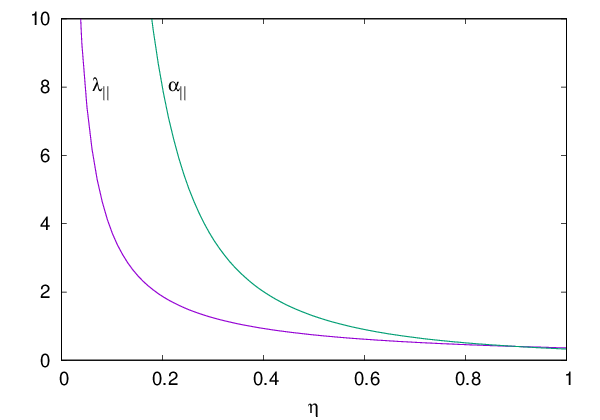
Both $\lambda_{\parallel}$ and $\alpha_{\parallel}$ diverge for $\eta\rightarrow 0$ as expected for a couple of metallic annulenes. On the other hand at $\eta=1$ we obtain the following results for the cyclacene molecule:

\begin{array}[]{l}\lambda_{\parallel}(1)\;=\;\frac{3}{2\sqrt{17}}b^{2}\;\approx\;0.363804\,b^{2},\\ \\ \alpha_{\parallel}(1)\;=\;\frac{33E\left(\frac{16}{17}\right)-K\left(\frac{16}{17}\right)}{8\pi\sqrt{17}}\,\frac{b^{2}}{t}\;\approx\;0.313082\,\frac{b^{2}}{t},\end{array}

showing its insulating character in the $xy$ plane and recovering the results found in a previous paper.Battaglia et al. 2018b

IV Discussion and conclusions.

In this paper we exploit the isomorphism between the $C_{n}$ group and the group of 1D translations with periodic Born von Kármán boundary conditions. We consider a finite ring of radius $R$ with open boundary conditions in the $(x,y)$ plane and a segment of length $L=2\pi R$ on a straight line with periodic boundary conditions. If we denote by $\phi$ the rotation angle around the centre of the ring in the e.g. counterclockwise direction, the arc length $s=R\phi$ on the ring is mapped on the coordinate, say $\zeta$ , on the line segment counted from e.g. its leftmost point: $0\leq\zeta<L$ . This can be viewed as rolling the ring on the straight line and in this sense all the points of the line can be mapped on the ring provided the angle $\phi$ is allowed to assume any real value. In the plane we can use a single complex coordinate $z=x+iy$ to describe any curve and in this way the equation of the ring is $z=R(\cos\phi+i\sin\phi)=R\exp(i\phi)=R\exp(is/R)$ . The point $P(z)$ of the ring is mapped on the point $P(\zeta)$ on the line, and we recover the complex position operator introduced in Ref. [Valença Ferreira de Aragão et al. 2019]. This mapping provides new insight into the nature of the complex position operator.

As far as the TPS is concerned, we can easily derive formulae for the thermodynamic limit for systems treated at non-correlated level, i.e. described by a Slater determinant. In particular a formula of Resta and coworkers is obtained in a different way from the original derivation.Sgiarovello, Peressi, and Resta 2001 More interesting a second formula, we called sum-over-states, for the TPS, equivalent to the Resta one in the limit of a complete basis, is also obtained. The latter allows for an interesting extension to the polarizability and to any quantity expressed as:

\langle\Phi_{0}\mu_{x}\left({\mathbf{H}}-E_{0}\right)_{\perp}^{K+1}\mu_{x}\Phi_{0}\rangle=S_{K}.

(52)

The quantities $S_{K}$ have been the object of much interest in the old days of perturbation theory Hirschfelder, Brown, and Epstein 1964 and are known as sum rules for oscillator strength. As already pointed out in Ref. [Valença Ferreira de Aragão et al. 2019] our approach using the complex position one-body operator can be applied to metallic systems avoiding the awkward “ $\ln 0$ ” singularity. This allows us to compute $\lambda$ for finite systems and study their behaviour when approaching the thermodynamic limit. As discussed in sections II.3.1 and II.3.2 the divergence of $\lambda$ is due to the partial filling of a band: this shows the equivalence of the two criteria for a non correlated system to be a conductor.

Finally, we want to stress the fact that, our approach is not confined to the treatment of periodic non interacting systems, although this was the subject of the present work. Indeed, once the ordinary position operator is replaced by the periodic complex-position one, it is possible to proceed exactly as in the case of OBC. It is worth noticing that the use of the periodic complex-position operator does not introduce complications for the numerical evaluation of its mean value, given that it is the square of a one-electron operator, exactly as in the case of the ordinary position operator. In all the cases we have investigated so far, the large-system qualitative behavior of the real and complex-position quantities is identical.

Concerning the treatment of correlated systems, we note that our approach does not present peculiar problems, given that one has to evaluate the mean value of the square of a one-electron operator and the machinery of quantum chemistry can be easily adapted to perform this task (playing attention to the fact that the operator is in this case complex). Actually, we have already treated correlated systems following the approach here reported.Valença Ferreira de Aragão et al. 2019 The difficulty, which is general for any approach, is mainly a “technical” one, since it is very hard to compute correlated wave-functions for systems having more than a dozen identical units. In a similar way, it will be possible to treat disordered systems, exactly in the same way done by using finite OBC formalism.Bendazzoli et al. 2010

Finally, we notice that the extension of the formalism to 2D and 3D systems will be the subject of future work.

Appendix 1

In this Appendix we show the vanishing of some matrix elements for systems enjoying the symmetry of the $C_{n}$ group. In particular we consider the matrix elements of Eq. (37) and use group theory arguments. Let us consider first the functions defined by the cartesian coordinates $x,y$ of a point $P$ in the ring, see the Supplementary material. We rewrite the latter as:

	$\displaystyle x(P)$	$\displaystyle=$	$\displaystyle\frac{R}{2}\left(e^{\frac{2\pi is}{L}}+e^{\frac{-2\pi is}{L}}\right),$		(53)
	$\displaystyle y(P)$	$\displaystyle=$	$\displaystyle-i\frac{R}{2}\left(e^{\frac{2\pi is}{L}}-e^{\frac{-2\pi is}{L}}\right),$		(54)

and, by comparison with Eq. (6), we realize that this couple of functions belong to the reducible representation E with $k=\pm 1$ . Therefore, expectation values of the dipole operators in the ring wavefunctions are vanishing. As concerns the second moments, we have:

$\displaystyle x^{2}(P)$	$\displaystyle=$	$\displaystyle\frac{R^{2}}{4}\left[e^{\frac{4\pi is}{L}}+e^{\frac{-4\pi is}{L}}+2\right],$	(55)
$\displaystyle y^{2}(P)$	$\displaystyle=$	$\displaystyle-\frac{R^{2}}{4}\left[e^{\frac{4\pi is}{L}}+e^{\frac{-4\pi is}{L}}-2\right],$	(56)
$\displaystyle xy(P)$	$\displaystyle=$	$\displaystyle-i\frac{R^{2}}{4}\left[e^{\frac{4\pi is}{L}}+e^{\frac{-4\pi is}{L}}\right].$	(57)

Therefore $xy$ and $x^{2}-y^{2}$ belong to the reducible representation $k=\pm 2$ , while $x^{2}$ and $y^{2}$ contain the A representation ( $x^{2}+y^{2}$ belong to A).

Appendix II

Here we report the eigenvalues and eigenvecors of the system of two annulenes coupled to form a cyclacene molecule when the parameter $\eta$ is equal to $1$

Table 6: Eigenvalues and normalized eigenvectors of two weakly bonded annulenes forming cyclacene for

\eta=1

\Upsilon=8+\eta^{2}+8\cos\frac{2\pi k}{n}

\begin{array}[]{l|c|c|}&&\\ &\mbox{eigenvector}\;1&\mbox{eigenvector}\;2\\ &&\\ \mbox{energy}&-t(\eta+\sqrt{\Upsilon})/2&t(\eta-\sqrt{\Upsilon})/2\\ &&\\ \sigma_{h}&+&-\\ \hline\cr&&\\ c_{1}&\frac{(\Upsilon-\eta\sqrt{\Upsilon})\sqrt{\Upsilon+\eta\sqrt{\Upsilon}}}{8\Upsilon\cos(k\pi/n)}&-\frac{(\Upsilon+\eta\sqrt{\Upsilon})\sqrt{\Upsilon-\eta\sqrt{\Upsilon}}}{8\Upsilon\cos(k\pi/n)}\\ &&\\ c_{2}&\frac{\sqrt{\Upsilon+\eta\sqrt{\Upsilon}}\sqrt{\Upsilon^{2}-\eta^{2}\Upsilon}(1-i\tan(k\pi/n))}{32\Upsilon\cos(k\pi/n)}&\frac{\sqrt{-\Upsilon+\eta\sqrt{\Upsilon}}\sqrt{\Upsilon^{2}-\eta^{2}\Upsilon}(1+i\tan(k\pi/n))}{32\Upsilon\cos(k\pi/n)}\\ &&\\ c_{3}&\frac{\sqrt{\Upsilon+\eta\sqrt{\Upsilon}}\sqrt{\Upsilon^{2}-\eta^{2}\Upsilon}(1-i\tan(k\pi/n))}{32\Upsilon\cos(k\pi/n)}&\frac{(\Upsilon+\eta\sqrt{\Upsilon})\sqrt{\Upsilon-\eta\sqrt{\Upsilon}}}{8\Upsilon\cos(k\pi/n)}\\ &&\\ c_{4}&\frac{(\Upsilon-\eta\sqrt{\Upsilon})\sqrt{\Upsilon+\eta\sqrt{\Upsilon}}}{8\Upsilon\cos(k\pi/n)}&\frac{(\Upsilon+\eta\sqrt{\Upsilon})\sqrt{\Upsilon-\eta\sqrt{\Upsilon}}}{8\Upsilon\cos(k\pi/n)}\\ &&\\ \hline\cr\hline\cr&&\\ &\mbox{eigenvector}\;3&\mbox{eigenvector}\;4\\ &&\\ \mbox{energy}&t(\sqrt{\Upsilon}-\eta)/2&t(\sqrt{\Upsilon}+\eta)/2\\ &&\\ \sigma_{h}&+&-\\ \hline\cr&&\\ c_{1}&\frac{(\Upsilon+\eta\sqrt{\Upsilon})\sqrt{\Upsilon-\eta\sqrt{\Upsilon}}}{8\Upsilon\cos(k\pi/n)}&-\frac{(\Upsilon-\eta\sqrt{\Upsilon})\sqrt{\Upsilon+\eta\sqrt{\Upsilon}}}{8\Upsilon\cos(k\pi/n)}\\ &&\\ c_{2}&\frac{\sqrt{-\Upsilon+\eta\sqrt{\Upsilon}}\sqrt{\Upsilon^{2}-\eta^{2}\Upsilon}(-1+i\tan(k\pi/n))}{32\Upsilon\cos(k\pi/n)}&\frac{-\sqrt{\Upsilon+\eta\sqrt{\Upsilon}}\sqrt{\Upsilon^{2}-\eta^{2}\Upsilon}(1-i\tan(k\pi/n))}{32\Upsilon\cos(k\pi/n)}\\ &&\\ c_{3}&\frac{\sqrt{-\Upsilon+\eta\sqrt{\Upsilon}}\sqrt{\Upsilon^{2}-\eta^{2}\Upsilon}(-1+i\tan(k\pi/n))}{32\Upsilon\cos(k\pi/n)}&\frac{\sqrt{\Upsilon+\eta\sqrt{\Upsilon}}\sqrt{\Upsilon^{2}-\eta^{2}\Upsilon}(1-i\tan(k\pi/n))}{32\Upsilon\cos(k\pi/n)}\\ &&\\ c_{4}&\frac{(\Upsilon+\eta\sqrt{\Upsilon})\sqrt{\Upsilon-\eta\sqrt{\Upsilon}}}{8\Upsilon\cos(k\pi/n)}&\frac{(\Upsilon-\eta\sqrt{\Upsilon})\sqrt{\Upsilon+\eta\sqrt{\Upsilon}}}{8\Upsilon\cos(k\pi/n)}\\ &&\\ \end{array}

V Appendix III

We detail here the reasons that led us to the choice of the imaginary exponential function in order to generalize the position operator to periodic systems. We limit ourselves to the 1-D case. These arguments had already been very schematically introduced in Ref. [Valença Ferreira de Aragão et al. 2019]. Let us consider the periodic interval (the “supercell”) $[0,L]$ , and let $x$ be the coordinate of a point belonging to the supercell: $x\in[0,L]$ . Let us call $q(x)$ the periodic position associated to the point of coordinate $x$ . We impose the three following general conditions to the periodic position:

1.

The function $q(x)$ must be a continuous periodic function of period $L$ :

$q(x+L)\;=\;q(x)\;,\;\forall x\;.$ (58)

In other words, $q(x)$ is translationally invariant in the supercell $[0,L]$ .
2.

The distance between two points, $x$ and $x+d$ , defined as the modulus of the difference between the corresponding complex positions, must be a function of $d$ alone, independent from $x$ :

$|q(x+d)-q(x)|^{2}\;=\;|q(d)-q(0)|^{2}\;.$ (59)
3.

For large values of $L$ , and $d$ fixed, we must obtain the ordinary distance between the two points:

$\lim_{L\rightarrow\infty}\,|q(d)-q(0)|^{2}\;=\;d^{2}\;.$ (60)

In the limit of an infinite supercell, one must recover the non-periodic result.

Condition 1 is manifestly satisfied choosing for $q(x)$ a function of the type

q(x)\;=\;\sum_{k=-\infty}^{\infty}a_{k}\,\exp\Bigl(\frac{i2\pi kx}{L}\Bigr)\;,

(61)

with $k$ integer. In order to investigate Condition 2, we compute the difference $q(x+d)\,-\,q(x)$ by using the previous equation. We obtain:

q(x+d)\,-\,q(x)\;=\;\sum_{k=-\infty}^{\infty}a_{k}\,\exp\Bigl(\frac{i2\pi kx}{L}\Bigr)\Bigl[\exp\Bigl(\frac{i2\pi kd}{L}\Bigr)-1\Bigr]\;.

(62)

We compute now the square of the distance between the points $x+d$ and $x$ , given by the square modulus of this quantity, $|q(x+d)-q(x)|^{2}$ . We get

|q(x+d)-q(x)|^{2}\;=\;\sum_{k=-\infty}^{\infty}\sum_{l=-\infty}^{\infty}\,a_{k}^{*}a_{l}\,\Bigl[\exp\Bigl(\frac{i2\pi(l-k)x}{L}\Bigr)\Bigr]\,\Bigl[\exp\Bigl(\frac{-i2\pi kd}{L}\Bigr)-1\Bigr]\,\Bigl[\exp\Bigl(\frac{i2\pi ld}{L}\Bigr)-1\Bigr]\;.

(63)

Among the three terms within square brackets, the only one containing $x$ is the first exponential factor. Therefore, in order to have a quantity not depending on $x$ , a sufficient condition is that all terms having $l\neq k$ in this equation vanish. This happens if only one term in Eq. (63) survives. Besides the trivial constant solution $q(x)=a_{0}$ , that does not lead to any physically acceptable result, let us consider a term $a_{j}$ different form zero. One can note that the corresponding $a_{-j}$ term is vanishing. This fact rules out real solutions of the type $q(x)=a\sin\bigr(\frac{2\pi jx}{L}\bigr)$ , or $q(x)=a\cos\bigr(\frac{2\pi jx}{L}\bigr)$ . We notice, moreover, that an exponential function is much easier to manipulate than a trigonometric one. Therefore, Condition 2 suggests the choice, for instance (let us assume $j=1$ ),

q(x)\;=\;a_{1}\,\exp\Bigl(\frac{i2\pi x}{L}\Bigr)\,+\,a_{0}\;.

(64)

It is worth noticing that the presence of the $a_{0}$ term does not invalidate the request that the quantity in Eq. (63) does not depend on $x$ , given that for $k=0$ or $l=0$ the second or the third term in square brackets is vanishing. Finally, a Taylor expansion of Condition 3 implies $a_{1}\,=\,\frac{L}{2\pi}$ . On the other hand, no physical constraints can be used to fix a value for $a_{0}$ , which is an arbitrary parameter related to the zero of the periodic position.

The above reasons suggest the definition

q(x)\;=\;\frac{L}{2\pi}\,\exp\Bigl(\frac{i2\pi x}{L}\Bigr)\;,

(65)

which is the one we use. The equivalent choice

q(x)\;=\;\frac{L}{2\pi}\,\exp\Bigl(\frac{-i2\pi x}{L}\Bigr)\;,

(66)

is also possible, being simply obtained from the previous one by a parity operation. The constant term $a_{0}$ can be chosen equal to $-\frac{L}{2\pi i}$ , in such a way to remove the constant term appearing in the exponential expansion.

Different non-equivalent choices are also possible for the integer $k$ , for instance, by choosing a different $a_{k}$ ( $k=\pm 2$ , or $k=\pm 3$ ,…) as the only non-zero term in Eq. (63) . In the limit of large boxes, all these choices lead to the same results and are therefore equivalent. However, the choice of $a_{1}$ (or equivalently, $a_{-1}$ ) are those that converge most quickly to the infinite-size limit and are therefore preferable. Notice that, as far as we have been able to find, no real solution satisfy all the three Conditions, 1-3. The characteristic of a complex nature is also shared by the operator $\hat{U}$ introduced in Resta’s formalism. The periodic position seems to be intrinsically complex.

Data Availability

The data that supports the findings of this study are available within the article.

References

Resta (1998) R. Resta, Phys. Rev. Lett. 80, 1800 (1998).
Resta and Sorella (1999a) R. Resta and S. Sorella, Phys. Rev. Lett. 82, 370 (1999a).
Resta (2002) R. Resta, Journal of Physics: Condensed Matter 14, R625 (2002).
Resta (2006) R. Resta, The Journal of Chemical Physics 124, 104104 (2006), https://doi.org/10.1063/1.2176604 .
Souza, Wilkens, and Martin (2000) I. Souza, T. Wilkens, and R. M. Martin, Phys. Rev. B 62, 1666 (2000).
Kohn (1964) W. Kohn, Phys. Rev. 133, A171 (1964).
Diaz-Marquez et al. (2018a) A. Diaz-Marquez, S. Battaglia, G. L. Bendazzoli, S. Evangelisti, T. Leininger, and J. A. Berger, J. Chem. Phys. 148, 124103 (2018a).
Brooke et al. (2018) L. Brooke, A. Diaz-Marquez, S. Evangelisti, T. Leininger, P.-F. Loos, N. Suaud, and J. A. Berger, J. Mol. Model. 24, 216 (2018).
Azor et al. (2019) M. E. Azor, L. Brooke, S. Evangelisti, T. Leininger, P.-F. Loos, N. Suaud, and J. A. Berger, SciPost Phys. Core 1, 1 (2019).
Evangelisti, Bendazzoli, and Monari (2010) S. Evangelisti, G. L. Bendazzoli, and A. Monari, Theor. Chem. Acc. 126, 257–263 (2010).
Monari and Evangelisti (2011) A. Monari and S. Evangelisti, “Physics and applications of graphene - theory,” (IntechOpen, Wien, 2011) Chap. Finite-Size Effects in Graphene Nanostructures.
Otto (1992) P. Otto, Phys. Rev. B 45, 10876 (1992).
Kudinov (1991a) E. K. Kudinov, Fizika Tverdogo Tela 33, 2306 (1991a).
Kudinov (1999) E. K. Kudinov, (1999), arXiv:9902361v1 .
Kudinov (1991b) E. K. Kudinov, Physics of the Solid State 41, 1450 (1991b).
Angeli, Bendazzoli, and Evangelisti (2013) C. Angeli, G. L. Bendazzoli, and S. Evangelisti, The Journal of Chemical Physics 138, 054314 (2013), https://doi.org/10.1063/1.4789493 .
Brea et al. (2013) O. Brea, M. El Khatib, C. Angeli, G. L. Bendazzoli, S. Evangelisti, and T. Leininger, Journal of Chemical Theory and Computation 9, 5286 (2013), pMID: 26592266, https://doi.org/10.1021/ct400453b .
El Khatib et al. (2014) M. El Khatib, T. Leininger, G. L. Bendazzoli, and S. Evangelisti, Chemical Physics Letters 591, 58 (2014).
Bendazzoli et al. (2014) G. L. Bendazzoli, M. El Khatib, S. Evangelisti, and T. Leininger, Journal of Computational Chemistry 35, 802 (2014), https://onlinelibrary.wiley.com/doi/pdf/10.1002/jcc.23557 .
El Khatib et al. (2015a) M. El Khatib, O. Brea, E. Fertitta, G. L. Bendazzoli, S. Evangelisti, and T. Leininger, The Journal of Chemical Physics 142, 094113 (2015a), https://doi.org/10.1063/1.4913734 .
Huran et al. (2016) A. W. Huran, T. Leininger, G. L. Bendazzoli, and S. Evangelisti, Chemical Physics Letters 664, 120 (2016).
Vetere et al. (2008) V. Vetere, A. Monari, G. L. Bendazzoli, S. Evangelisti, and B. Paulus, The Journal of Chemical Physics 128, 024701 (2008), https://doi.org/10.1063/1.2822286 .
Bendazzoli et al. (2008) G. L. Bendazzoli, S. Evangelisti, A. Monari, B. Paulus, and V. Vetere, Journal of Physics: Conference Series 117, 012005 (2008).
Monari, Bendazzoli, and Evangelisti (2008) A. Monari, G. L. Bendazzoli, and S. Evangelisti, The Journal of Chemical Physics 129, 134104 (2008), https://doi.org/10.1063/1.2987702 .
Vetere et al. (2009) V. Vetere, A. Monari, A. Scemama, G. L. Bendazzoli, and S. Evangelisti, The Journal of Chemical Physics 130, 024301 (2009), https://doi.org/10.1063/1.3054709 .
Bendazzoli, Evangelisti, and Monari (2011) G. L. Bendazzoli, S. Evangelisti, and A. Monari, International Journal of Quantum Chemistry 111, 3416 (2011), https://onlinelibrary.wiley.com/doi/pdf/10.1002/qua.23047 .
Bendazzoli, Evangelisti, and Monari (2012) G. L. Bendazzoli, S. Evangelisti, and A. Monari, International Journal of Quantum Chemistry 112, 653 (2012), https://onlinelibrary.wiley.com/doi/pdf/10.1002/qua.23036 .
El Khatib et al. (2015b) M. El Khatib, O. Brea, E. Fertitta, G. L. Bendazzoli, S. Evangelisti, T. Leininger, and B. Paulus, Theoretical Chemistry Accounts 134, 29 (2015b), https://doi.org/10.1007/s00214-015-1625-7 .
Fertitta et al. (2015) E. Fertitta, M. El Khatib, G. L. Bendazzoli, B. Paulus, S. Evangelisti, and T. Leininger, The Journal of Chemical Physics 143, 244308 (2015), https://doi.org/10.1063/1.4936585 .
Battaglia et al. (2018a) S. Battaglia, H.-A. Le, G. L. Bendazzoli, N. Faginas-Lago, T. Leininger, and S. Evangelisti, International Journal of Quantum Chemistry 118, e25569 (2018a), https://onlinelibrary.wiley.com/doi/pdf/10.1002/qua.25569 .
Diaz-Marquez et al. (2018b) A. Diaz-Marquez, S. Battaglia, G. L. Bendazzoli, S. Evangelisti, T. Leininger, and J. A. Berger, The Journal of Chemical Physics 148, 124103 (2018b), https://doi.org/10.1063/1.5017118 .
Huran et al. (2018) A. W. Huran, N. Ben Amor, S. Evangelisti, S. Hoyau, T. Leininger, and V. Brumas, The Journal of Physical Chemistry A 122, 5321 (2018), pMID: 29775056, https://doi.org/10.1021/acs.jpca.7b12187 .
Sgiarovello, Peressi, and Resta (2001) C. Sgiarovello, M. Peressi, and R. Resta, Phys. Rev. B 64, 115202 (2001).
Valença Ferreira de Aragão et al. (2019) E. Valença Ferreira de Aragão, D. Moreno, S. Battaglia, G. L. Bendazzoli, S. Evangelisti, T. Leininger, N. Suaud, and J. A. Berger, Phys. Rev. B 99, 205144 (2019).
Tavernier et al. (2020) N. Tavernier, G. L. Bendazzoli, V. Brumas, S. Evangelisti, and J. A. Berger, The Journal of Physical Chemistry Letters 11, 7090 (2020), pMID: 32787331, https://doi.org/10.1021/acs.jpclett.0c01684 .
Tavernier et al. (2021) N. Tavernier, G. L. Bendazzoli, V. Brumas, S. Evangelisti, and J. A. Berger, Theoretical Chemistry Accounts 140, 106 (2021).
Alves et al. (2021) E. Alves, G. L. Bendazzoli, S. Evangelisti, and J. A. Berger, Phys. Rev. B 103, 245125 (2021).
Dresselhaus, Dresselhaus, and Jorio (2008) M. S. Dresselhaus, G. Dresselhaus, and A. Jorio, Group Theory: Application to the Physics of Condensed Matter (Springer-Verlag Berlin Heidelberg, 2008).
Calais et al. (1995) J. L. Calais, B. T. Pickup, M. Deleuze, and J. Delhalle, European Journal of Physics 16, 179 (1995).
Craven (1985) B. D. Craven, The Journal of the Australian Mathematical Society. Series B. Applied Mathematics 26, 362–374 (1985).
Kutzelnigg (2007) W. Kutzelnigg, Journal of Computational Chemistry 28, 25 (2007), https://onlinelibrary.wiley.com/doi/pdf/10.1002/jcc.20470 .
(42) Strictly this holds for $n>2$ .
Resta and Sorella (1999b) R. Resta and S. Sorella, Phys. Rev. Lett. 82, 370 (1999b).
Hirschfelder, Brown, and Epstein (1964) J. O. Hirschfelder, W. B. Brown, and S. T. Epstein, Recent Developments in Perturbation Theory, edited by P.-O. Löwdin, Advances in Quantum Chemistry, Vol. 1 (Academic Press, 1964) pp. 255 – 374.
(45) Wolfram Research, Inc., “Mathematica, Version 12.1,” Champaign, IL, 2020.
Battaglia et al. (2018b) S. Battaglia, H.-A. Le, G. L. Bendazzoli, N. Faginas-Lago, T. Leininger, and S. Evangelisti, International Journal of Quantum Chemistry 118, e25569 (2018b), https://onlinelibrary.wiley.com/doi/pdf/10.1002/qua.25569 .
Bendazzoli et al. (2010) G. L. Bendazzoli, S. Evangelisti, A. Monari, and R. Resta, The Journal of Chemical Physics 133, 064703 (2010), https://doi.org/10.1063/1.3467877 .

	$\displaystyle\!\!\!\left<\tilde{\psi}_{k\gamma}\middle\|1-\hat{P}_{occ}\middle\|\tilde{\psi}_{k\gamma}\right>=$
	$\displaystyle=\left<\tilde{\psi}_{k\gamma}\middle\|\tilde{\psi}_{k\gamma}\right>-\sum_{\gamma^{\prime}}\left<\tilde{\psi}_{k\gamma}\middle\|\psi_{k\pm 1\gamma^{\prime}}\right>\left<\psi_{k\pm 1\gamma^{\prime}}\middle\|\tilde{\psi}_{k\gamma}\right>$
	$\displaystyle=R^{2}\left(1-\sum_{\gamma^{\prime}}\left\|\int_{0}^{d}u_{k\gamma}(s)\,u_{k\pm 1\gamma^{\prime}}(s)ds\right\|^{2}\right),$		(26)

	$\displaystyle\left\|\left<u_{k,\gamma}\middle\|u_{k\pm 1,\eta}\right>\right\|^{2}=$	(29)
$\displaystyle=$	$\displaystyle\delta_{\gamma\eta}\pm\delta_{\gamma\eta}\frac{2\pi}{nd}\left(\left<u_{\gamma}\middle\|\frac{\partial u_{\eta}}{\partial K}\right>+\left<\frac{\partial u_{\eta}}{\partial K}\middle\|u_{\gamma}\right>\right)+$
	$\displaystyle+\left(\frac{2\pi}{nd}\right)^{2}\left<u_{\gamma}\middle\|\frac{\partial u_{\eta}}{\partial K}\right>\left<\frac{\partial u_{\eta}}{\partial K}\middle\|u_{\gamma}\right>+$
	$\displaystyle+\frac{\delta_{\gamma\eta}}{2}\!\!\left(\frac{2\pi}{nd}\right)^{2}\!\!\left(\left<u_{\gamma}\middle\|\frac{\partial^{2}u_{\eta}}{\partial K^{2}}\right>+\left<\frac{\partial^{2}u_{\eta}}{\partial K^{2}}\middle\|u_{\gamma}\right>\right)+$
	$\displaystyle+\;O(n^{-3})$
$\displaystyle=$	$\displaystyle\delta_{\gamma\eta}\>+\>\left(\frac{2\pi}{nd}\right)^{2}\left<u_{\gamma}\middle\|\frac{\partial u_{\eta}}{\partial K}\right>\left<\frac{\partial u_{\eta}}{\partial K}\middle\|u_{\gamma}\right>+\;$
	$\displaystyle-\delta_{\gamma\eta}\>\left(\frac{2\pi}{nd}\right)^{2}\left<\frac{\partial u_{\gamma}}{\partial K}\middle\|\frac{\partial u_{\gamma}}{\partial K}\right>+\;O(n^{-3}),$

$\displaystyle\mathbf{\alpha}$	$\displaystyle=$	$\displaystyle\left<(\hat{X}\pm i\hat{Y})\Phi\middle\|(\mathbf{H}_{K}-E_{0})_{\perp}^{-1}\middle\|(\hat{X}\pm i\hat{Y})\Phi\right>\>=$	(37)
	$\displaystyle=$	$\displaystyle\left<\hat{X}\Phi\middle\|(\mathbf{H}_{K}-E_{0})_{\perp}^{-1}\middle\|\hat{X}\Phi\right>+$
		$\displaystyle+\left<\hat{Y}\Phi\middle\|(\mathbf{H}_{K}-E_{0})_{\perp}^{-1}\middle\|\hat{Y}\Phi\right>+$
		$\displaystyle\pm i\left<\hat{X}\Phi\middle\|(\mathbf{H}_{K}-E_{0})_{\perp}^{-1}\middle\|\hat{Y}\Phi\right>+$
		$\displaystyle\mp i\left<\hat{Y}\Phi\middle\|(\mathbf{H}_{K}-E_{0})_{\perp}^{-1}\middle\|\hat{X}\Phi\right>.$

	$\displaystyle\frac{\left\|\left<u_{k,\gamma}\middle\|u_{k\pm 1,\eta}\right>\right\|^{2}}{\epsilon_{k\pm 1,\eta}-\epsilon_{k,\gamma}}=\frac{\delta_{\gamma\eta}}{\epsilon_{\eta}(K)-\epsilon_{\gamma}(K)}\;+$
	$\displaystyle\quad\quad\quad+\frac{2\pi}{nd}\frac{\left<u_{\gamma}\middle\|\frac{\partial u_{\eta}}{\partial K}\right>\left<\frac{\partial u_{\eta}}{\partial K}\middle\|u_{\gamma}\right>}{\epsilon_{\eta}(K)-\epsilon_{\gamma}(K)}+$
	$\displaystyle\quad\quad\quad+\delta_{\gamma\eta}\frac{2\pi}{nd}\frac{\partial\epsilon_{\eta}}{\partial K}\,\frac{1}{(\epsilon_{\eta}(K)-\epsilon_{\gamma}(K))^{2}}+$
	$\displaystyle\quad\quad\quad+\left(\frac{2\pi}{nd}\right)^{2}\,\frac{\partial\epsilon_{\eta}}{\partial K}\,\frac{\left<u_{\gamma}\middle\|\frac{\partial u_{\eta}}{\partial K}\right>\left<\frac{\partial u_{\eta}}{\partial K}\middle\|u_{\gamma}\right>}{(\epsilon_{\eta}(K)-\epsilon_{\gamma}(K))^{2}}+$
	$\displaystyle\quad\quad\quad-\delta_{\gamma\eta}\left(\frac{2\pi}{nd}\right)^{2}\!\!\frac{\left<\frac{\partial u_{\gamma}}{\partial K}\middle\|\frac{\partial u_{\gamma}}{\partial K}\right>}{\epsilon_{\eta}(K)-\epsilon_{\gamma}(K)}+O(L^{-3}).$		(42)