A Coupled Alpha Complex
Abstract
The alpha complex is a subset of the Delaunay triangulation and is often used in computational geometry and topology. One of the main drawbacks of using the alpha complex is that it is non-monotone, in the sense that if it is not necessarily (and generically not) the case that the corresponding alpha complexes satisfy . The lack of monotonicity may introduce significant computational costs when using the alpha complex, and in some cases even render it unusable. In this work we present a new construction based on the alpha complex, that is homotopy equivalent to the alpha complex while maintaining monotonicity. We provide the formal definitions and algorithms required to construct this complex, and to compute its homology. In addition, we analyze the size of this complex in order to argue that it is not significantly more costly to use than the standard alpha complex.
1 Introduction
The alpha complex [13] is a parametrized triangulation constructed over point clouds. It is widely used in computer graphics [20], computational geometry [21, 22], topological data analysis (TDA) [24], and other fields. Given a point cloud , the alpha complex is a -dimensional simplicial complex consisting of a subset of the faces in the Delaunay triangulation of . In TDA, one of its main uses is as a substitute for the Čech complex (the nerve of the balls of radius centered at ), justified by the fact that the alpha and the Čech complexes are homotopy equivalent. While the Čech complex is highly useful to develop the theory and intuition in TDA (especially in probabilistic analysis [4, 19]), using the alpha complex in applications is significantly more efficient computationally. The Čech complex contains many -simplexes , and those can appear in any dimension. On the other hand, the alpha complex contains simplexes only up to dimension , and it can be shown [26] that there are at most many of them. Moreover, for generic random point clouds, it can be shown [17] that the alpha complex has only many simplexes. Since computing homology or persistent homology, for example, requires cubical time in the number of simplexes, such a difference in the complex size can be crucial.
One of the main drawbacks of the alpha complex is the following. For any finite we have a natural inclusion . However, the same is not true in general for the alpha complex. In other words, adding new points to an existing alpha complex, requires us to re-calculate the entire complex. There are various scenarios where the lack of such an inclusion can prevent us from using alpha complexes. For example:
- 1.
Computing zigzag-persistence [8]. As opposed to the standard persistent homology that is (commonly) computed over filtrations, in zigzag persistence the inclusion relations may go in different ways. For example, suppose that we have a sequence of point clouds , with no inclusion relation, and we wish to find cycles that persist throughout this sequence. Using the Čech complex, we can take the sequence
and compute its zigzag persistence barcode, for example. However, we are currently not able to do so using alpha complexes, and the computational implications are substantial.
- 2.
Cycle registration in persistent homology [25]. We recently presented a new framework for identifying matching persistent cycles between pairs of simplicial filtrations. For example, suppose that we have two point clouds . We can use the Čech filtration to compute two persistent modules and . Our goal is to find pairs of persistent-cycles (classes) in and that represent the “same topological phenomenon” (which we define rigorously in [25]). Our solution heavily relies on the inclusions , and specifically on the images of the induced maps in homology. Here as well, we cannot use the alpha complex. At the same time, using the Čech complex (or the Vietoris-Rips) becomes infeasible for rather small sample sizes.
In order to resolve this fundamental issue, we present here a new construction we call the coupled alpha complex and denote by . This is a new “hybrid” complex defined over pairs of finite point clouds . The key properties of this new complex are: (a) It is homotopy equivalent to the alpha complex ; (b) It satisfies the desired inclusions that the alpha complex misses, i.e., and ; (c) The total number of simplexes in this complex is (still smaller compared to Čech), and for random point clouds we can show that the expected size goes down to .
Related work.
In [2] the authors introduce the selective Delaunay complex, defined for a subset of excluded points. This complex is a subset of simplexes for which there exists a sphere that includes and its interior excludes . The alpha and Čech complexes are extremal cases obtained by choosing and , respectively. In this paper we suggest a similar yet different construction. While in a selective Delaunay complex all the simplexes are induced by a fixed subset , in our case, we have two distinct sets and of excluding points. Specifically, it is a subset of simplexes for which there exist two concentric spheres, one that includes and its interior excludes , and one that includes and its interior excludes . In addition, while in general the selective Delaunay complex includes only ), ours also includes and .
In [3] the authors define the Relative Delaunay-Čech complex which is a complex designed for computing the persistent homology of relative to , where . This complex is a subset of the Delaunay triangulation of , which is similar in spirit to the way we construct the coupled alpha complex in Section 4. One of the main differences between these constructions is the filtration values assigned to the simplexes. In the relative Delaunay-Čech complex, the filtration value of each is , while for it is the radius its minimal bounding sphere. On the other hand, in the coupled alpha complex the filtration values are computed in a top down fashion, with no distinction between the sets and . More generally, while the relative Delaunay-Čech complex is designed specifically for computing relative persistent homology, the coupled alpha complex is a general-purpose tool that serves as a “bridge” between arbitrary alpha complexes. Moreover, one can obtain the relative Delaunay-Čech complex (up to homotopy equivalence) from the coupled alpha complex, by assigning some of the simplexes with a filtration value of zero. Finally, the formalism we present here, simplifies the derivation of a probabilistic upper bound on the complex size, presented in Section 5.
Paper outline.
In Section 2 we give a brief introduction for the terms and the structures discussed in this paper. In Sections 3 and 4 we introduce the main contribution of this paper – the coupled alpha complex. We present the formal definition and provide a two-step computation scheme. Finally, in Section 5 we provide a probabilistic upper bound for the expected size of the coupled alpha complex, in the case where the points cloud is generated at random.
2 Preliminaries
In this section we give a brief introduction to simplicial complexes, homology and persistent homology. For more details [12, 14, 16, 18, 28].
2.1 Simplicial homology
An abstract simplicial complex over a set , is a collection of finite subsets that is closed under inclusion, i.e., if and , then, . The elements of are called simplexes and their dimension is determined by their size minus one. For , we say that is a face of , and is a co-face of of co-dimension , where .
Homology.
Homology is a topological-algebraic structure that describes the shape of a topological space by its connected components, holes, cavities, and generally -dimensional cycles (see Figure 1). Loosely speaking, given a topological space , is an abelian group generated by elements that correspond to the connected components of ; similarly is generated by “holes” in ; is generated by the “cavities” or “bubbles” in . Generally, we can define the group generated by the non-trivial -dimensional cycles of . A -dimensional cycle can be thought of as the boundary of a -dimensional object (i.e. with the interior excluded).

Formally, let be a simplicial complex. The -dimensional chain group is a free abelian group generated by the -dimensional simplexes in . In this article we will use coefficients, and therefore is a vector space. The elements of are formal sums of -simplexes called chains. The boundary homomorphism is defined as follows. If is a chain representing a single -simplex, then , where denotes that is a -dimensional face of . For general chains , extends linearly, i.e. . It can be shown that for every , and the sequence
is known as a chain complex. Next, we define the subgroups
so that . The group is known as the -cycle group (i.e. chains whose boundary is zero) and as the -boundary group (i.e. -cycles that are boundaries of -dimensional chains). The -th homology group is then defined as the quotient group,
In other words, the -th homology group consists equivalence classes of -dimensional cycles who differ only by a boundary (called homological cycles). The ranks of the homology groups, called the Betti numbers, are denoted .
As mentioned earlier, intuitively speaking, the generators (or basis) of correspond to the connected components of , corresponds to the holes in , and are the cavities. The definitions provided above are for simplicial homology, while other notions of homology groups can be defined for a much larger classes of topological spaces (see [18]). The intuition, however, is similar.
In addition to homology, throughout the paper we will also use the following two terms which can be defined for simplicial homology as well as the more general notions of homology.
Simplicial maps and induced homomorphisms.
Let and be simplicial complexes and let be a simplicial map, i.e., for . Then homology theory provides a sequence of induced functions denoted , that map -cycles in to -cycles in .
Homotopy Equivalence.
This is a notion of similarity between spaces that is weaker than homeomorphism. Loosely speaking, two topological spaces and are homotopy equivalent, denoted , if one can be continuously deformed into the other. In particular, homotopy equivalence between spaces implies similar homology, i.e. if , then for all .
2.2 Geometric complexes
Simplicial complexes are the fundamental building blocks in many TDA methods, where they are used for approximating geometric shapes using discrete structures. In this section we present a few special types of geometric complexes commonly used in TDA.
Definition 2.1 (Čech Complex).
Let be a finite set of points in a metric space. The Čech complex of with radius , denoted by , is an abstract simplicial complex, constructed using the intersections of balls around ,
where is a ball of radius centered at .
Definition 2.2 (Vietoris-Rips Complex).
Let be a finite set of points in a metric space. The Vietoris-Rips complex of with radius , denoted by , is an abstract simplicial complex, constructed by pairwise intersections of balls,
In other words, all the points in are within less than distance from each other.


The Čech and Rips complexes are the most extensively studied complexes in TDA. The Rips complex is commonly used in applications (see for example [10]) due to its simple definition that depends on pairwise distances only. The Rips complex can be also viewed as an approximation for the Čech complex by the following relation [9, 15],
The construction of the Čech complex is a bit more intricate, hence it is slightly less popular in applications. However, the Čech complex plays a central role in many theoretical results, especially in the random setting (see for example [19, 27, 4, 1, 5]). This largely due to the fact that the Čech complex is homotopy equivalent to the ball cover inducing it due to the Nerve Lemma which we state in the following.
Definition 2.3 (Nerve of a covering).
Let be a topological space and let be a cover of . The Nerve of , denoted by , consists of all finite subsets such that,
Note that by definition is an abstract simplicial complex.
Lemma 2.4 (Nerve Lemma [7]).
Let be a topological space and let be a good cover of , i.e. for every the set is either contractible or empty. Then, the nerve is homotopy equivalent to .
A direct result of the Nerve Lemma is the following corollary.
Corollary 2.5.
Let be a finite set of points. Then,
Corollary 2.5 implies that the homology groups of and are isomorphic. Hence, they can be used interchangeably when trying to prove a result concerning their homotopy type or homology groups.
The next complex we discuss, the alpha complex, serves as a basis for the construction of the coupled alpha complex introduced in Section 3. The alpha complex is homotopy equivalent to the Čech complex, but with much fewer simplexes. Let be a finite set of points in a metric space . The Voronoi cell of with respect to is defined as
In addition, we define the Voronoi ball of with respect to , as
| (1) |
Definition 2.6 (Alpha complex).
Let be a finite set of points in a metric space. The Alpha Complex of with parameter , denoted by , is defined as the nerve of all the Voronoi balls, i.e.
By the Nerve Lemma, we have that , and in particular they have the same homology.
Throughout this article we will assume that a given point set is in general position, defined as follows.
Definition 2.7 (General Position).
A finite set () is said to be in general position, if for every of size ,
- 1.
The points of do not lie on a -dimensional flat.
- 2.
No point of lies on the circumsphere of .
In this case, the alpha complex can be realized as a (geometric) simplicial complex embedded in (as opposed to the Čech complex), i.e. it also satisfies the following geometric condition,
In other words, if two embedded simplexes intersect, they must intersect along a common face. In addition, for large enough, becomes identical to the Delaunay triangulation, defined as follows.
Definition 2.8 (Delaunay Triangulation).
Let be a finite set. The Delaunay Triangulation of , denoted by , is a triangulation of such that the circumsphere of each -simplex in the triangulation does not contain any point of .
Note that for sets in general position the Delaunay triangulation is unique (see [6]).
Alpha complex computation.
While algorithms for constructing the Čech and Rips complexes are derived directly from their definitions, an algorithm for the Alpha complex is derived from its definition in a rather dual way, based on the following proposition (see Figure 3).
Proposition 2.9 ([13]).
Let be a finite set in general position. Then,


Given , we first compute its Delaunay triangulation, which by Proposition 2.9 equals to . Next, the identification of the subset of simplexes that are in , is done in a top down fashion, starting from the top dimensional simplexes and going downwards.
Let and denote the filtration value of by
| (2) |
In other words, is the minimal value for which the Voronoi balls of intersect. The problem of finding can be translated into the problem of finding the radius of the minimal -sphere that includes the points of and does not contain any points of in its interior. Thus we obtain the following optimization problem,
| (3) |
for arbitrary . Computing (3) directly is hard. Instead, can be computed in a top-down fashion. Define to be the set of all co-faces of co-dimension . In [6] the authors show that equals to one of two possible values: if the minimal circumsphere of does not contain any point of in its interior, then equals to the radius of that sphere. Otherwise, . For more information and an explicit algorithm for the computation of the alpha complex see [6].
2.3 Persistent homology
Persistent homology is one of the fundamental tools used in TDA, and can be thought of as a multi-scale version of homology. While homology is calculated for a single space , persistent homology is applied to a filtration. Let be a topological space and consider a filtration , so that for all we have . As is increased, holes can be created and/or filled in, introducing changes to the homology. Persistent homology is used to track these changes.
For , the inclusion induces a homomorphism between the homology groups. These induced maps enable us to track the evolution of homology classes throughout the filtration, from the point when they are first formed (born) to the point when they become boundaries, and hence trivial (die). The algebraic structure tracking this evolution is called a persistence module, denoted . In [28] it was shown that has a unique decomposition into basis elements called persistence intervals. Intuitively, each persistence interval tracks a single -cycle from birth to death. For each persistence cycle we denote by the point (value of ) where is first created, and by the point where becomes trivial. The entire lifetime interval is denoted by . In most TDA applications, once persistent homology is calculated one outputs a numerical summary in the form of a barcode or a persistence diagram (see Figure 4). These are two equivalent ways to visually represent the collection of pairs for all persistence intervals.

An example where persistent homology is used is in the context of geometric complexes. Here, the filtration parameter is the radius , and the persistent homology provides a summary for all the cycles that appear at different scales. Given point cloud data, we can compute the persistent homology of either the Čech or the Rips filtration in order to extract information about the topological space underlying the data.
3 The Coupled Alpha Complex
In this section, we introduce the coupled alpha complex denoted , where are finite sets. We will define this complex in such a way that it meets the following requirements,
In other words, this complex includes both alpha complexes of each of the sets separately, and is homotopy equivalent to the alpha (or Čech) complex over their union. In addition, we will show that it maintains low computational costs compared to the Čech and Rips complexes over the union of points.
The coupled alpha complex is constructed using the same building blocks as the alpha complex. Recall that given a subset , the alpha complex is defined as the nerve of the Voronoi cells . The coupled alpha complex is defined using two different Voronoi tessellations, each related to a different set of points, denoted and (see Figure 5). The formal definition of this complex is the following.
Definition 3.1 (Coupled Alpha Complex).
Let be a pair of finite subsets and let . Define the following sets
The coupled alpha complex generated by and with parameter is defined as
Note that the (standard) alpha complex on is given by taking the nerve of .

Remark 3.2.
For points in general position in , the dimension of the alpha complex is always . However, it is important to notice that the coupled alpha complex is -dimensional. This stems, for example, from configurations where the intersection point of Voronoi cells in lies in the interior of a Voronoi cell in . Nonetheless, by the nerve lemma we have .
The definition above implies that the following inclusion relations hold,
In addition, by the Nerve Lemma 2.4 we have the following.
Lemma 3.3.
Let be a pair of finite subsets of and let . Then,
Proof.
The elements of are all convex sets (as intersections of convex sets). Hence, by the Nerve Lemma 2.4
and . ∎
In conclusion, we have the following relations, where the new complex substitutes . The dashed arrows represent the missing inclusion relations between and that are replaced by the inclusion maps into .
4 Constructing the Coupled Alpha Complex
In the following section we provide an algorithm for calculating the coupled alpha filtration . The computation is divided into two steps. We start by finding , i.e. the set of all possible simplexes that may appear in the coupled alpha filtration. Then, we calculate the filtration values for each possible simplex.
4.1 Computing
Assume that and are assigned with a given ordering. The key idea is to lift these sets from to in such a way that the lifted sets and lie in parallel hyperplanes. We proceed by computing the regular -dimensional Delaunay triangulation of and its induced simplicial complex denoted . Finally, we show that is isomorphic to .
Let be the natural projection, i.e. . Let be a simplex such that . The projected simplex of , denoted by , is defined by:
| (4) |
Let be an ordered pair of finite subsets of . Define and .

Throughout, we will assume that the sets are in coupled general position, defined as follows.
Definition 4.1 (Coupled General Position).
Let be two finite sets and define and . and are said to be in coupled general position if:
- 1.
and are in general position (in ), and
- 2.
for every and such that , no point of lies on the circumsphere of .
This assumption implies that the vertices of the Voronoi tessellation of are at the intersection of exactly Voronoi cells (see the proof of Proposition 4.2 below). Note that for generic random point processes, this assumption holds with probability . This is true, since for any of size that contains points in both sets , the probability that a point lies on the circumsphere of is zero (since the circumsphere is a set of -measure).
In the following, we argue that the coupled general position assumption is sufficient for the Delaunay triangulation to be uniquely-defined. Recall that for points in general position the Delaunay triangulation is unique. From Definition 2.7, taking , the conditions hold for sets that are composed of points from both sets and by the coupled general position assumption. However, general position is violated, for (or ) of size , as such sets lie on a -dimensional flat (the containing hyperplane). However, these sets are ignored to get a valid triangulation - a subdivision of the convex hull of into -simplexes that form a simplicial complex - which is unique and dual to the Voronoi diagram of .
Proposition 4.2.
Let be an ordered pair of finite subsets of . Then,
where the right-hand-side is the abstract simplicial complex generated by projecting the coordinates of the faces of using (4).
Proof.
First we show that if then . Denote by and by , and assume that both and are not empty. Since
Let be such that and . In order to show that , we need to show that the following condition holds.
Define such that and for arbitrary and . For this choice of we have that for all and ,
and for every and
where is an arbitrary point. Similarly, for every and
Hence, which implies that is non-empty and therefore .
So far we assumed that are non-empty. Next, assume without loss of generality, that is empty. In that case
Define such that and for an arbitrary point . For this choice of we get that for all and
implying that,
which leads to
Hence, which completes the proof of the first direction.
Next, we need to show that if then . Denote by , i.e., the simplex that is obtained by applying to the points of and to the points of . By assumption, there exists such that
Denote . If , then
hence,
Similarly, we can show
Thus, , which completes the proof. ∎
To conclude, in this section we showed that Algorithm 1 produces the complex .
4.2 Computing filtration values
Once we computed , we proceed to determining the filtration value attached to each simplex. Recall that in the alpha complex, the filtration value attached to each simplex is given by the radius of the minimal circumsphere that does not contain any other points in its interior (3). We will define the filtration value of a simplex in a similar fashion. Let and . We define the filtration value of to be:
| (5) |
The optimization problem stated in (5) can be translated to a problem where the unknown variable is the center (in ) of two concentric -dimensional open balls and that are empty in the following sense. The first ball includes the points on its boundary and it does not include any other point of in its interior. Similarly, the second ball includes the points on its boundary and it does not include any other point of in its interior. In general, there can be an infinite number of such pairs of balls (see Figure 7).
For each such pair we can define to be the radius of the bigger ball. Then, we set , where the minimum is taken over all possible pairs . In the following we state the optimization problem whose solution is the filtration value of a given simplex, and present algorithm for computing the minimizer of this problem.

4.2.1 Optimization problem
Let , such that both and are not empty and assume that and . Let
| (6) |
The filtration value of is the solution for the following optimization problem:
| (7) |
where and are two arbitrary points.
Note that in the case where is empty, i.e. , the solution for (7) coincides with the filtration value of as a simplex in the alpha complex of and vice versa.
The minimizer of (7) must lie in the intersection of the Voronoi cells of the vertices of . This constraint makes the optimization problem hard to solve. Instead, we will first solve the following relaxed version of the problem
| (8) |
where we replaced with , respectively. Note that since . The solution for the relaxed problem will play a central role in identifying the filtration value of , i.e. the solution for (7), as we will see in the following.
4.2.2 Relaxed optimization problem
In the following, we reformulate the optimization problem (8). Assume an arbitrary ordering on and . The set consists of all points that satisfy the following equations,
Similarly, is the set of all points that satisfy
The solution we seek lies in , hence, we combine the equations above into a single system. For simplicity, we write the equations in a matrix form. Define,
Note that since the points are in general position, the rows of are linearly independent, i.e. . Using the above notation, the optimization problem can now be written in the following way
| (9) |
Note that for all we have and , and the choice of in (9) is arbitrary. Using the fact that a solution for a linear system can be expressed as a sum of a solution for the homogeneous system and a particular solution, we reformulate the optimization problem in the following way,
| (10) |
where is a particular solution, i.e. , and is the matrix whose columns are an orthonormal basis of .
We derive the solution in the following way. Denote by the objective function in (10), then its derivative with respect to is
Recalling that consists of orthonormal columns, the minimizer of (10) is one of the following three terms,
or
or
where is the center of the minimal circumsphere of (in ).
In practice, we compute the first two candidates , measure their distances to and and then check which is the right solution according to the following claim.
Lemma 4.3.
Denote
The solution for (9), denoted by , is given by
where is the radius of the minimal circumsphere of (in ).
Proof.
The proof relies on the fact that the objective in (9) is convex. There are three cases we should address. The first case is when . Here, since is the global minimum of in , we have that , and similarly . Therefore, we conclude that , which implies that . The second case, when is similar. The last case is when both and . Here, the minimum of (10) is a boundary point, i.e. a value that satisfies
(otherwise, the minimizer must be either of and , in contradiction to the assumption). Under this constraint, (10) is exactly the optimization problem for finding the minimal circumsphere of . Hence, the minimizer in that case satisfies , which gives . ∎
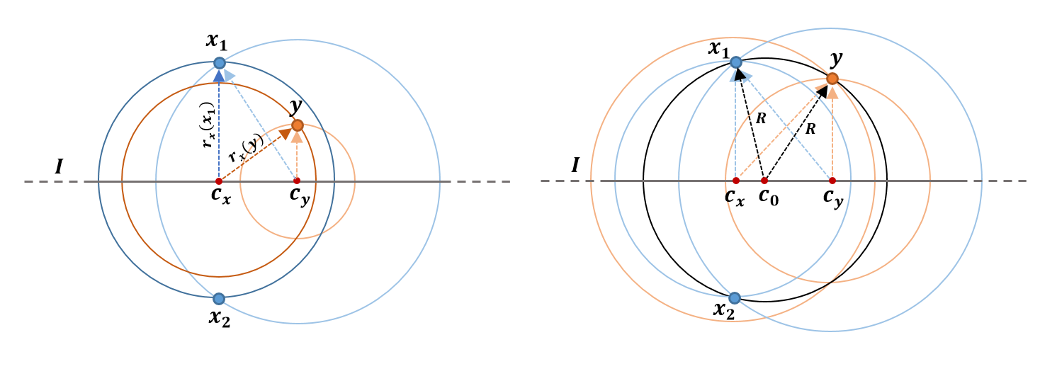
4.2.3 Back to the non-relaxed problem
Determining the solution for the non-relaxed problem (7) can be done in a top-down fashion, similarly to the calculation of the filtration values for the alpha complex [6]. Adopting the terminology of [6], we define the following condition.
Let and let be a face of (of co-dimension ). Let be the minimizer of (8) for . Define to be the open ball with center and radius for arbitrary , and let be its bounding sphere. Similarly define and .
We say that the ordered pair satisfies the coupled Gabriel condition if both , and . Let be the set of all co-faces of (of co-dimension ). If for every , the pair satisfies the coupled Gabriel condition, then we say that is a coupled Gabriel simplex. This property will enable us to determine whether the solution of (8) for identifies with the solution of (7), as we suggest in the following lemma (see Figure 9).
Lemma 4.4.
Let be a coupled Gabriel simplex. Then, the filtration value of is given by .
Proof.
Our goal is to show that the solutions of (7) and (8) for are the same. In the previous section we found the minimizer for the relaxed problem (8). If we can show that , then also minimizes (7), and therefore .
Let , and without loss of generality, suppose that . The coupled Gabriel condition implies that for an arbitrary . Since this is true for every we conclude that . Similarly, we can show that , concluding the proof. ∎
The following lemma provides a way to determine the filtration value of in the case where the conditions of Lemma 4.4 are not satisfied, i.e. the coupled Gabriel condition does not hold for .
Lemma 4.5.
Let , and suppose there exists such that does not satisfy the coupled Gabriel condition. Then,
Proof.
For every , is a face of , which implies that , hence . Assume that . In that case, the solution of (7) must lie in the interior of . Let be the minimizer that corresponds to . Since (7) is a convex optimization problem and is a convex polyhedron, also solves the relaxed optimization problem (8) for (since the relaxed constraint is the affine hull of the non-relaxed constraint ). This is in contradiction to not being coupled Gabriel simplex. ∎


To conclude, in this section we introduced a way to determine the filtration values for the simplexes in . Algorithm 2 produces the filtration values for all the simplexes in sequentially, starting from top dimensional simplexes and moving downwards. The function filtrationValue, first appearing in line 5, returns the minimizer of the relaxed problem (10) for given simplex. Note that in practice, we index the vertices of the sets in the following way and , so that given a simplex it is easy to split it to and such that .
Remark 4.6.
In [3] the authors present the relative Delaunay-Čech complex, , in order to compute the relative-persistent homology , where . This complex is defined by similar building blocks as ours, computing is identical to the first step in computing all possible simplexes of . However, the filtration values are different. For , the filtration value of a simplex is the radius of the minimal bounding sphere of (as in the Čech complex), while the filtration values of all simplexes are set to . Thus, making all cycles generated by chains in trivial.
5 The Number of Simplexes in a Random Coupled Alpha Complex
In the general (non-random) case, the number of simplexes in a Delaunay triangulation in -dimensions is [26]. Since the coupled alpha complex is a subset of the Delaunay triangulation, it contains at most -simplexes. However, for a generic random data set the Delaunay triangulation contains simplexes [11]. Unfortunately, this bound cannot be applied directly to the coupled alpha complex, since the data points are restricted to two parallel hyperplanes.
In this section we provide an upper probabilistic bound for the size of the coupled alpha complex, when the points are generated by a Poisson point process.
Let be a compact set and let be a sequence of i.i.d. random variables uniformly distributed in . Let be a Poisson random variable independent of the -s. Then, we define
We say that is a homogeneous Poisson point process with intensity .
Let be a compact set, and let and be two independent homogeneous Poisson processes on with intensity . Denote by the number of -simplexes in . Our main result states that the expected value of is of order . In addition, let and assume , where
Proposition 5.1.
If , then the expected number of -simplexes in is
I.e.,
for , where are constants that do not depend on .
Proof.
In order to prove 5.1, we first characterize the -simplexes in in spherical-like coordinates. We use the change of variables to prove that . Then, we bound the number of -simplexes by
We start by defining explicitly. Let . Denote . Assume that and for (both sets non-empty). First, we define the following,
where and are arbitrary points. Next, define
and
| (11) |
Finally, we can express in terms of the above functions,
| (12) |
Recall that in our case , and and are two independent homogeneous Poisson processes with intensity . Applying Mecke’s formula (see Theorem A.1 in the Appendix A) twice for (12) yields,
| (13) |
where and are sets of uniform random variables in of size and , respectively, and are independent of and .
Conditioning on , and using the fact that and are independent, yields
| (14) |
Therefore, using (11), we have
| (15) |
Next, we compute (15) in terms of integrals. We start by defining a transformation that takes the vertices of a -simplex in to a coordinate system where they are expressed in terms of the minimal pair of open balls defined in Section 4.2.
Let for . Let be the map defined by
| (16) |
where , for arbitrary , and are points on the -dimensional unit sphere. First note that the number of degrees of freedom in the codomain equals , which is equal to that of the domain. The point is a unique point (see Lemma B.1 in the Appendix A), hence the map is a bijection. Note that for we have
which implies that the homology does not change if is increased. Hence, we can limit our analysis for simplexes with and . We can then bound (15) in the following way,
| (17) |
where is the volume of the unit ball in .
From (16), we have that the Jacobian satisfies Hence, we can rewrite the RHS of (17) in the following way,
Finally, using the changes of variables apply the following change of variables , , and the definition of the incomplete gamma function , we have
| (18) | ||||
where
To conclude, substituting (18) into (13) we have that the number of -simplexes is bounded by
where we used the fact that . Hence, we conclude that the total number of -simplexes centered at in is bounded from above by
The following result given in [17] is the number of -simplexes in the alpha complex (when ) of a Poisson point process with intensity , that are centered at ,
| (19) |
By using (19), we can bound the number of simplexes from below by the number of simplexes in , since . Hence, we conclude that
∎
Appendix
Appendix A Meck’s Formula
The following theorem is a result of Palm theory for Poisson point processes.
Theorem A.1 (Mecke’s formula).
Let be a metric space, let be a probability density on , and let be a random Poisson process on with intensity . Let be a measurable function defined for all finite subsets with . Then
| (20) |
where the sum is over all subsets of size , and is a set of iid random variables in with density , independent of .
Appendix B Random Hyperplanes Lemma
Let be two subsets, such that and , for . Denote
In other words, and are all the points that equidistant from the points and respectively.
Lemma B.1.
Let be sets of iid points sampled from a distribution with a density in . The following holds almost surely.
and
Proof.
Assume an arbitrary ordering on and . The intersection can be expressed as the set of all points that solve the system, , where
Since the points of are iid , with a density in , they are almost surely in a coupled general position (Definition 4.1). Hence, (since its rows are linearly independent) and there is a unique solution to the system, i.e. a point. Note that if we apply similar arguments to the part of the matrix that contains only or only, we get and . ∎
References
- [1] Antonio Auffinger, Antonio Lerario, and Erik Lundberg. Topologies of random geometric complexes on riemannian manifolds in the thermodynamic limit. International Mathematics Research Notices, apr 2020.
- [2] Ulrich Bauer and Herbert Edelsbrunner. The Morse theory of Čech and Delaunay complexes. Transactions of the American Mathematical Society, 369(5):3741–3762, 2017.
- [3] Nello Blaser and Morten Brun. Relative Persistent Homology. In 36th International Symposium on Computational Geometry (SoCG 2020), volume 164 of Leibniz International Proceedings in Informatics (LIPIcs), pages 18:1–18:10, 2020.
- [4] Omer Bobrowski. Homological connectivity in random Čech complexes. arXiv preprint arXiv:1906.04861, 2019.
- [5] Omer Bobrowski and Primoz Skraba. Homological percolation: The formation of giant k-cycles. International Mathematics Research Notices, dec 2020.
- [6] Jean-Daniel Boissonnat, Frédéric Chazal, and Mariette Yvinec. Geometric and topological inference, volume 57. Cambridge University Press, 2018.
- [7] Karol Borsuk. On the imbedding of systems of compacta in simplicial complexes. Fundamenta Mathematicae, 35:217–234, 1948.
- [8] Gunnar Carlsson, Vin De Silva, and Dmitriy Morozov. Zigzag persistent homology and real-valued functions. In Proceedings of the 25th annual symposium on Computational geometry, pages 247–256. ACM, 2009.
- [9] Vin de Silva and Robert Ghrist. Coverage in sensor networks via persistent homology. Algebraic & Geometric Topology, 7(1):339–358, apr 2007.
- [10] Vin De Silva and Robert Ghrist. Homological sensor networks. Notices of the American mathematical society, 54(1), 2007.
- [11] Rex A. Dwyer. Higher-dimensional voronoi diagrams in linear expected time. Discrete & Computational Geometry, 6(3):343–367, 1991.
- [12] Edelsbrunner, Letscher, and Zomorodian. Topological persistence and simplification. Discrete & Computational Geometry, 28(4):511–533, nov 2002.
- [13] Herbert Edelsbrunner. Alpha shapes – a survey. Tessellations in the Sciences, 01 2010.
- [14] Herbert Edelsbrunner and John Harer. Persistent homology – a survey. Discrete & Computational Geometry - DCG, 453, jan 2008.
- [15] Herbert Edelsbrunner and John L. Harer. Computational topology: an introduction. AMS Bookstore, 2010.
- [16] Herbert Edelsbrunner and Dmitriy Morozov. Persistent homology: Theory and practice. In European Congress of Mathematics Kraków, 2 – 7 July, 2012, pages 31–50. European Mathematical Society Publishing House, jan 2014.
- [17] Herbert Edelsbrunner, Anton Nikitenko, and Matthias Reitzner. Expected sizes of Poisson–Delaunay mosaics and their discrete Morse functions. Advances in Applied Probability, 49(3):745–767, 2017.
- [18] Allen Hatcher. Algebraic topology. Cambridge University Press, Cambridge, 2002.
- [19] Matthew Kahle. Random geometric complexes. Discrete & Computational Geometry, 45(3):553–573, jan 2011.
- [20] Michael Krone, Barbora Kozlíková, Norbert Lindow, Marc Baaden, Daniel Baum, Julius Parulek, H-C Hege, and Ivan Viola. Visual analysis of biomolecular cavities: State of the art. Computer Graphics Forum, 35(3):527–551, 2016.
- [21] Jie Liang, Herbert Edelsbrunner, Ping Fu, Pamidighantam V. Sudhakar, and Shankar Subramaniam. Analytical shape computation of macromolecules: I. molecular area and volume through alpha shape. Proteins: Structure, Function, and Bioinformatics, 33(1):1–17, 1998.
- [22] Jie Liang, Clare Woodward, and Herbert Edelsbrunner. Anatomy of protein pockets and cavities: Measurement of binding site geometry and implications for ligand design. Protein Science, 7(9):1884–1897, 1998.
- [23] Mathew Penrose. Random geometric graphs, volume 5. Oxford University Press Oxford, 2003.
- [24] Pratyush Pranav, Herbert Edelsbrunner, Rien van de Weygaert, Gert Vegter, Michael Kerber, Bernard J. T. Jones, and Mathijs Wintraecken. The topology of the cosmic web in terms of persistent Betti numbers. Monthly Notices of the Royal Astronomical Society, 465(4):4281–4310, 11 2016.
- [25] Yohai Reani and Omer Bobrowski. Cycle registration in persistent homology with applications in topological bootstrap. arXiv preprint arXiv:2101.00698, 2021.
- [26] Raimund Seidel. The upper bound theorem for polytopes: an easy proof of its asymptotic version. Computational Geometry, 5(2):115–116, 1995.
- [27] D. Yogeshwaran, Eliran Subag, and Robert J. Adler. Random geometric complexes in the thermodynamic regime. Probability Theory and Related Fields, 167(1-2):107–142, nov 2015.
- [28] Afra Zomorodian and Gunnar Carlsson. Computing persistent homology. Discrete & Computational Geometry, 33(2):249–274, nov 2004.