What makes you unique?
Abstract
This paper proposes a uniqueness Shapley measure to compare the extent to which different variables are able to identify a subject. Revealing the value of a variable on subject shrinks the set of possible subjects that could be. The extent of the shrinkage depends on which other variables have also been revealed. We use Shapley value to combine all of the reductions in log cardinality due to revealing a variable after some subset of the other variables has been revealed. This uniqueness Shapley measure can be aggregated over subjects where it becomes a weighted sum of conditional entropies. Aggregation over subsets of subjects can address questions like how identifying is age for people of a given zip code. Such aggregates have a corresponding expression in terms of cross entropies. We use uniqueness Shapley to investigate the differential effects of revealing variables from the North Carolina voter registration rolls and in identifying anomalous solar flares. An enormous speedup (approaching 2000 fold in one example) is obtained by using the all dimension trees of Moore and Lee, 1998 to store the cardinalities we need.
1 Introduction
An individual data point, such as one representing a person, can often be identified by specifying even a small subset of its variables. For instance, a large fraction of US residents are uniquely identified by just their date of birth, zip code, and gender (Sweeney, 2000; Golle, 2006). The website https://amiunique.org/ will examine some signature variables in your browser and report whether you are uniquely identified among the millions of participants. See Gómez-Boix et al., 2018 for a description.
Variables are not equally powerful for the purpose of identifying an individual, and the variables that provide the most information for one person might not be very informative for another. It can also happen that two or more variables specified together can be much more identifying than we might surmise given their individual strengths for identifying people. The joint specification can also be less informative due to associations between variables such as near duplicates.
In this paper we propose a way to measure how important a variable is for identifying one specific subject in a set of data. Our definition of importance is based on Shapley value from economic game theory (Shapley, 1953). An important variable is one that, when revealed for a subject, greatly reduces the number of subjects who could match it. This measure takes account of which other variables might also have been revealed, and so it depends on the full joint distribution in the data set not just one or a few marginal distributions of the data. It does not assume that any set of variables necessarily provides a unique identification of the subject, as might fail to happen for twins.
The game theoretic formulation provides a principled way to aggregate subject-specific importances to variable importance measures for the whole data set or for subsets of special interest, using the additivity property of Shapley value. The measure is an extension of the cohort Shapley measure that Mase et al., 2019 use to quantify variable importance for black box functions.
Other things being equal, a more identifying variable is one that is more worth concealing for privacy purposes, or more valuable for personalization. That said, our measure is not designed for settings like differential privacy (Dwork, 2008) where one seeks privacy guarantees. We use it instead for exploratory purposes.
An outline of the paper is as follows. Section 2 introduces our notation, reviews Shapley value and defines the uniqueness Shapley values of each input variable for a given subject. Variables with greater Shapley value are more identifying. Section 3 shows that the uniqueness Shapley value can be related to an entropy measure. When aggregated to an entire data set, the uniqueness Shapley value for variable is a weighted sum of the conditional empirical entropies of variable given all subsets of variables not including . When we aggregate only over a proper subset of subjects the resulting Shapley value expression replaces entropies by cross-entropies linking the empirical distribution on the subset to the full data set. A naive implementation of aggregated uniqueness Shapley value will have a cost that is quadratic in the number of subjects. Section 4 describes the all dimension trees of Moore and Lee, 1998 that we have found give an enormous speedup making the difference between feasible and infeasible computation in some of our examples. Section 5 explores a solar flare dataset from Dua and Graff, 2017. We treat solar regions with the most extreme and potentially dangerous flares as anomalies and then, as a step towards explaining those anomalies, look at which variables most identify them. Section 6 looks at voter registration data from the state of North Carolina. We compare the extent to which race, age, gender and other variables serve to identify voters. Section 7 gives conclusions and discusses some further issues.
2 Notation and background
We suppose that there are categorical variables measured on each of subjects. Subject is described by a vector with components for . The set of all subjects is denoted and the set of all variables is .
To begin, suppose that there is a target subject , and we want to know what variables identify subject . For every subset of variables let be the tuple . Then we define the cohort
of all subjects who match subject on every variable in the set . By convention, and no cohort is empty because they all include . The size of a cohort is the cardinality
We consider variable to be important for identifying subject if is typically much smaller than for . In that case, knowledge of refines the cohort containing subject by a large factor. There are different cohorts into which might be included, and we will use Shapley value to incorporate them all.
To simplify some of our expressions, we introduce some notational short forms. The set is written as . When then we write for . The set of all subsets of is written . When is a finite set, then is its cardinality.
2.1 Shapley value
The Shapley value from game theory can be used to allocate value to the members of a team that produced the value. In our context, the team will be made up of variables whose values are specified, and the value will be defined by how much subject is identified.
We work with a value function where is the value created by the team , and we suppose that we are given for all . The total value created by the team is , and the problem is to make a fair allocation to members . The fair share for member is denoted by . Shapley, 1953 had these axioms:
- 1)
(Efficiency) ,
- 2)
(Symmetry) if whenever then ,
- 3)
(Dummy) if whenever then and
- 4)
(Additivity) if two games have value functions and and shares and then the game with values must have shares .
The fair shares depend strongly on the incremental value of variable given that variables are already included. It is convenient to use
| (1) |
to represent this incremental value. Shapley, 1953 finds that there is a unique set of shares (called Shapley values) that satisfy his four axioms. They are
| (2) |
Another way to describe is to build a set from to by adding the variables in a random order. At some point variable appears with a set of previously introduced variables. Then is the average of taken over all variable orders.
We see from equation (2) that only value differences affect . It is often convenient to take . If that does not hold we can replace every by without changing any of the .
2.2 Uniqueness Shapley
The value function we choose for identifying subject is
| (3) |
This definition satisfies . The smaller the cardinality of , the more has served to identify subject . One unit of corresponds to information that halves the size of the cohort containing subject . We quantify the importance of to the identifiability of subject via the Shapley value derived from the value function in (3). The extent to which revealing identifies subject depends on any previously identified variables for . The uniqueness Shapley value combines all of these contributions in a way consistent with game theory. Those contributions take the form
after cancellation of .
The uniqueness Shapley value function is the cohort Shapley value function of Mase et al., 2019 after the within-cohort average of a response variable is replaced by the cardinality of the cohort.
Proposition 1.
The uniqueness Shapley value satisfies with if and only if for all .
Proof.
If , then and from this we find that . If for all then for making and . Conversely, suppose that but for some . Then from which . This provides a contradiction because there cannot be any compensating negative value differences to bring the Shapley value down to zero. ∎
Now suppose that we want to quantify the importance of variable to the whole set of subjects. The additivity axiom of Shapley value makes it natural to sum those values. For interpretability we scale that sum to an average over subjects taking
| (4) |
as our global measure of the cardinality importance of variable .
For an arbitrary non-empty subset of subjects we can also define
| (5) |
Suppose for instance that encodes the gender of subject . We can then define a set consisting of all the subjects with one of the genders in the data set and then describes the extent to which gender identifies people of the given gender. This is not necessarily zero even though gender is constant over because the Shapley values are defined on the entire subject set . For some other feature such as age in years we can then measure the extent to which identifies subjects of a given gender and see how this varies as we change the set to each gender in turn.
3 Relationship to information theory
It is natural to consider entropy as a measure of how informative a feature is for identification. Gómez-Boix et al., 2018 report entropy values for individual variables in their browser fingerprint data. Here we introduce some information theoretic quantities and show that uniqueness Shapley value aggregated over subjects is equivalent to entropy when the features are independent. More generally, aggregating the uniqueness Shapley measure yields a linear combination of conditional entropies. Aggregates over proper subsets of subjects involve cross-entropies.
For a categorical variable with we write the entropy of both and as . For disjoint the conditional entropy of given is
By the chain rule for entropy (Cover and Thomas, 2006, Theorem 2.2.1)
We will work with the entropy of sub-vectors of and for this we write when the distribution of is understood from context. Similarly, denotes . For we may abbreviate the conditional entropy to .
3.1 Relationship to entropy
Let be the empirical distribution on with
| (6) |
For , let be the marginal distribution of under (6) and for let be the marginal distribution of under (6).
We say that two or more variables are independent in the data if they are independent random variables under (6). Exact independence is quite unlikely to occur but it provides an interpretable baseline via Shannon’s entropy.
Proposition 2.
Proof.
Consider subject . Because is independent of we find that is independent of . This means that for all ,
and then based on its expression as an average over permutations of incremental values. Now aggregating over subjects,
As usual, the proper interpretation of is zero. If all the variables are independent, then they all have a uniqueness Shapley value equal to their entropy. The connection to entropy goes further.
Proposition 3.
The global uniqueness Shapley value for variable is
| (7) |
where the conditional entropies are computed for a random vector with the empirical distribution (6).
Proof.
For we have . Then
and so . ∎
Because conditional entropies are non-negative and is the entropy of under , we have the bracketing inequality
| (8) |
Noting that we find for that
| (9) |
with found by switching indices. For ,
It may seem counterintuitive that larger entropy corresponds to greater power to identify subjects. If a variable takes two levels, say 0 and 1, then the distribution with greatest entropy is the one that gives them each probability . Revealing that variable provides ‘1 bit’ of cohort reduction. If instead there is a 90:10 split for some variable then 10% of the population find that their cohort size is greatly reduced by 10-fold () but 90% find their cohort size reduced by the much lower amount, . This is about 11% and , so the average number of bits is .
The largest possible global uniqueness Shapley value for a binary predictor variable is . In the solar flare example of Section 5 we will see for a binary predictor and a set of anomalous observations.
3.2 Relationship to cross entropy
For two distributions and on a discrete set the relative entropy (Kullback-Leibler distance) from to is
Similarly, the cross entropy of relative to is
It is very common to write these expressions with symbols and reversed, but in our setting, the second argument needs to be the empirical distribution from (6) that we have labeled . For distribution , we use marginal distributions , and analogous to the quantities that we have used previously for .
Proposition 4.
The uniqueness Shapley values for subset of subjects at (5) can be written
| (10) |
where is the uniform distribution on for .
Proof.
First, by definition
Next, for a set ,
This sum can be rewritten over as long as we divide out the multiplicity for each among the for yielding
Here is the number of subjects in that match on the features in . As is the uniform distribution over for , , i.e., the proportion of subjects in that match on the features in . Therefore
With this formulation we can see that
3.3 Duplicate and redundant variables
If some other variable is equivalent to variable , then it must have the same uniqueness Shapley value. The extreme version of this is that the second variable could have been copy-pasted from the first one by accident. More plausibly there could be two variables like a person’s email address and cell phone number that have very nearly a one to one relationship in a data set of transactions.
Let’s look at in the special case where all . Then and and we find that
This is strictly smaller than the value in (9) unless is constant in the data in which case both are zero.
Next we consider the effect of introducing this duplicate on . We get
The coefficient of has decreased from to while the coefficient of has increased from to .
A redundant variable is one that can be perfectly identified based on some subset of other variables. Like a duplicated variable, the redundant ones do not get a uniqueness Shapley value of zero.
3.4 Database key
Suppose that one of the variables uniquely identifies each subject. That is, we never have unless . We can think of this as the key variable in a database or even the row number in a data frame. The presence of this variable forces (it’s largest possible value) for every subject. For each subject, whenever the key is in .
We can look at where is a set of variables and now suppose that we introduce a database key with index . For each of the prior orders in which variable could have been included there are positions at which the new variable could be introduced. If variable is introduced after variable then the incremental value is unchanged. If variable is introduced before variable then the new incremental value for variable is . Therefore introducing the key changes the uniqueness Shapley value for one subject to
| (11) |
because of the possible insertion points preserve the incremental value while the others remove it. Equation (3.4) holds for with corresponding to . The sum in (3.4) is taken over subsets of the original variables exclusive of both variable and the posited key variable .
After introducing the key variable, the contribution of is downweighted by a factor of , which ranges from for to for . The average value of this factor over sets is
Other things being equal we might expect that introducing the database key will halve the other variables’ uniqueness Shapley values. Variables that get their importance mostly from for small are less affected by the key, and variables that get their importance mostly from for large will lose more than half of their uniqueness Shapley values.
4 All dimension trees
It would require time to compute by naively checking which subjects match the target on a particular subset of features . For a naive calculation of the uniqueness Shapley, we would therefore need to compute times for each combination of feature and subjects to calculate each . Therefore, the full run time of the naive implementation of uniqueness Shapley would be . For a reasonably large number of subjects, the factor can be computationally prohibitive even when is not large. To improve upon the naive implementation, we employ a more suitable data structure: the all dimension tree of Moore and Lee, 1998.
The all dimension tree is optimized for tasks similar to calculating , i.e., generating contingency tables. The basic structure takes categorical data and constructs a tree where each branch corresponds to a particular “feature equals value” query, and the subsequent node stores the count of all subjects for whom that query and all preceding queries in the tree are true. To compute for a given pair, you start at the root of the tree and follow the branches corresponding to queries for all , and the count stored in the resulting node would be . Therefore, with such a tree structure, we only require time to compute which no longer scales with the number of subjects. Note that the same tree can be used for all subjects, so it need not be constructed more than once for a single data set.
A naive version of this structure would generally require a prohibitive amount of memory, thereby rendering the computational savings moot even for relatively small . The innovation of the all dimension tree comes from its techniques to reduce memory requirements especially in the common cases of sparsity and correlated features. They use several different methods to achieve this goal which are not relevant to the scope of this discussion except that they succeed in reducing the memory cost. For example, for binary features, the memory requirement is in the worst case compared to in the dense naive implementation, and it can achieve in the best case. Performance closer to the best case is achieved when features are distributed more unevenly and are more correlated, resulting in a sparser distribution. The time to initially construct the all dimension tree is also linear in and while worst-case exponential in , it is not worse than our dependence to in the Shapley calculation. This makes our overall implementation of uniqueness Shapley using all dimension trees . A speed up by a factor of . We use the all dimension tree Python implementation developed by Ding, 2018.
| Data | n | d | ADTree | Standard |
|---|---|---|---|---|
| Solar Flare | 1,066 | 9 | 5.30 | 54.55 |
| Dare County Census | 30,921 | 5 | 1.91 | 2,522.40 |
| Durham County Census | 253,563 | 5 | 16.46 | 32,426.91 |
| North Carolina Census | 7,538,125 | 5 | 362.51 | n/a |
For a reasonably large number of features , this implementation is no longer computationally feasible. In those cases, a Monte Carlo approximation must be employed as in Maleki et al., 2013. The all dimension tree structure can also be adapted for large to reduce its memory dependence at the cost of only approximately calculating which is also discussed in Moore and Lee, 1998. Our present examples did not have such very large . An implementation of uniqueness Shapley can be found on our GitHub: https://github.com/cohortshapley/uniquenessshapley.
5 Solar flare data example
Many data sets have a few entries that are anomalies, such as outliers. There have been many efforts to detect anomalies and others to explain them. For a survey of anomaly detection, see Chandola et al., 2009. Jacob et al., 2020 provide the Exathlon benchmark for anomaly explanation methods, aimed at time series. They include a method based on marginal entropies.
In this section we look at the solar flare data set from the UC Irvine repository (Dua and Graff, 2017). Some of the solar flares have been marked as unusual (anomaly detection). We consider uniqueness Shapley as a way to understand which variables make the anomalous data most unique. We must add that finding an identifying variable for an anomaly is a kind of association and is not necessarily causal. For instance, an unusual person’s social security number is very identifying but is unlikely to be causal.
We use the second solar flare data set from the UC Irvine repository because it is said to be more reliable. It describes regions on the surface of the sun. There are 10 categorical predictors and 3 responses indicating the number of common (C class), moderate (M class) and severe (X class) solar flares in each region over a 24 hour period. Severe flares are 100 times as strong as moderate ones which in turn are 10 times as strong as common ones. The M class flares can cause radio blackouts or endanger astronauts. There are also numerical gradations within these classes. See https://www.nasa.gov/mission_pages/sunearth/news/X-class-flares.html.
Some of those solar regions are much more interesting than others. All but five of them had no severe flares. Of those five, one had two severe flares. Four of the regions had three or more flares rated moderate or severe, so we consider those too. We will use uniqueness Shapley to study these anomalies in terms of the categorical predictors of the data set. The first nine categorical predictor variables are described in Table 2. A tenth variable, about the area of the largest spot, was constant for all 1066 regions. We omit that variable and work with others.
| Variable | Levels |
|---|---|
| Modified Zurich class | (A, B, C, D, E, F, H) |
| Largest spot size | (X, R, S, A, H, K) |
| Spot distribution | (X, O, I, C) |
| Activity | (1 = reduced, 2 = unchanged) |
| Evolution | (1 = decay, 2 = no growth, 3 = growth) |
| Prior 24 hr activity | (1 = no M1s, 2 = one M1, 3 = multiple M1s) |
| Historically-complex | (1 = yes, 2 = no) |
| This pass | (1 = yes, 2 = no) |
| Area | (1 = small, 2 = large) |
The first two columns of Table 3 show entropy and cardinality Shapley values for the 9 predictors in the solar flare data. Zurich and large spot are the most identifying. Area is least identifying. In this data, many of the uniqueness Shapley values are below their corresponding marginal entropy.
| Variable | Entropy | Shapley | Common | Moderate | Severe |
|---|---|---|---|---|---|
| Zurich | 1.64 | 1.37 | 1.72 | 1.62 | 1.81 |
| Large Spot | 1.52 | 1.55 | 1.69 | 1.62 | 1.23 |
| Spot Dist | 1.16 | 0.92 | 1.17 | 1.34 | 1.49 |
| Activity | 0.43 | 0.45 | 0.73 | 0.67 | 0.86 |
| Evolution | 0.90 | 1.17 | 0.98 | 0.98 | 0.85 |
| Prev Activ | 0.18 | 0.16 | 0.33 | 0.43 | 0.93 |
| Complex | 0.67 | 0.77 | 0.69 | 0.69 | 0.29 |
| This Pass | 0.38 | 0.35 | 0.15 | 0.11 | 0.03 |
| Area | 0.12 | 0.07 | 0.22 | 0.43 | 1.36 |
The last three columns of Table 3 shows cardinality Shapley for some subsets of solar regions of increasingly anomalous nature. They are those with at least one common flare, at least one moderate flare, and, finally, at least one severe flare. The area variable which is so unimportant globally becomes ever more identifying for these anomalies. So does ‘previous activity’. These variables are associated with anomalous solar behavior in that the more extreme the behavior, the more identifying these become.
6 North Carolina voter registration data
Here we consider a real world demographic example in the vein of Sweeney’s original work (Sweeney, 2000). The state of North Carolina publishes voting and demographic information about all of its registered voters each election. Some information is withheld to maintain privacy such as exact birth dates, exact addresses, and social security numbers. From the available features, we looked at zip code, age, race, gender, and political party affiliation for registered voters in the state. Summary uniqueness Shapley values and baseline marginal entropy values can be found in Table 4. There we can see that the relative ordering of the uniqueness Shapley values is consistent with the entropy values, but that we have large positive deviations for zip code and age. All variables had Shapley value greater than their entropy. Recall that the lower bound on the Shapley value is one fourth of the entropy, since .
| Zip Code | Race | Party | Gender | Age | |
|---|---|---|---|---|---|
| Shapley | 8.58 | 1.22 | 1.48 | 1.17 | 5.39 |
| Entropy | 6.08 | 1.08 | 1.14 | 0.92 | 4.24 |
In Table 5, we can see the average uniqueness Shapley values for various subpopulations of the state. Some patterns follow logically from the relative class sizes, as for example, members of races that make up a smaller percentage of the population have larger uniqueness Shapley values for race on average. Clearly membership in a less common class should help to uniquely identify someone. Other noticeable patterns highlight the effects of the correlation structure not captured by the marginal entropy measures. For example, the average cardinality value for race decreases for older age cohorts.
| Subgroup | Zip Code | Race | Party | Gender | Age | % Pop. |
| Democratic | 8.44 | 1.54 | 1.31 | 1.14 | 5.47 | 36 |
| Libertarian | 8.15 | 1.16 | 6.65 | 1.14 | 4.54 | 1 |
| Republican | 8.76 | 0.72 | 1.51 | 1.15 | 5.50 | 30 |
| None | 8.57 | 1.32 | 1.51 | 1.22 | 5.23 | 33 |
| Female | 8.58 | 1.18 | 1.46 | 0.97 | 5.46 | 49 |
| Male | 8.61 | 1.15 | 1.49 | 1.20 | 5.40 | 42 |
| No Answer | 8.42 | 1.76 | 1.53 | 2.24 | 4.91 | 8 |
| White | 8.75 | 0.53 | 1.58 | 1.09 | 5.52 | 63 |
| Black | 8.28 | 1.70 | 1.14 | 1.10 | 5.35 | 21 |
| Asian | 7.56 | 5.44 | 1.44 | 1.09 | 5.01 | 1 |
| Native American | 7.64 | 5.14 | 1.40 | 1.01 | 5.13 | 1 |
| No Answer | 8.45 | 2.27 | 1.54 | 1.91 | 4.94 | 10 |
| Age | 8.49 | 1.52 | 1.52 | 1.26 | 4.63 | 25 |
| 32–48 | 8.48 | 1.33 | 1.50 | 1.20 | 5.22 | 25 |
| 48–63 | 8.61 | 1.13 | 1.46 | 1.15 | 5.33 | 25 |
| 63 | 8.71 | 0.90 | 1.44 | 1.09 | 6.34 | 25 |
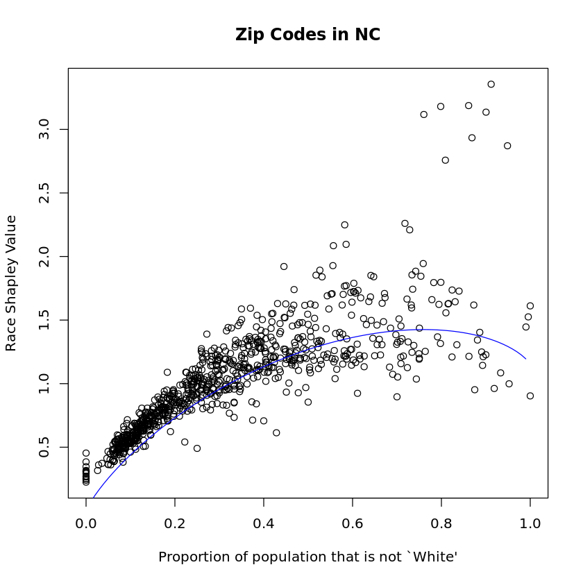
To further investigate the relationship between class imbalance and the uniqueness Shapley value, we look at zip code defined subpopulations in Figure 1. We plot the Shapley value for race versus the proportion of the population that does not identify as white. There are a handful of large positive outliers to this trend. Upon further inspection, we can note that these are all zip codes with a very high proportion of American Indian voters.
We can also measure the effect of feature granularity on the uniqueness Shapley values. Instead of recording location by zip code, we can coarsen it to the county level or even the whole state. The results for this adjusted dataset are in Table 6. The uniqueness Shapley values for the other variables are not sensitive to this coarsening. Similarly, instead of considering each age by year, we can coarsen the grouping level to five or ten or years and again we see no meaningful changes outside of the expected reduction in the age feature, even if we lump all ages into one bucket.
| Location | Race | Party | Gender | Age | |
| Zip Code | 8.58 | 1.22 | 1.48 | 1.17 | 5.39 |
| County | 5.55 | 1.27 | 1.50 | 1.19 | 5.43 |
| State | 0.00 | 1.32 | 1.53 | 1.19 | 5.45 |
| Zip code | Race | Party | Gender | Age | |
| Single year | 8.58 | 1.22 | 1.48 | 1.17 | 5.39 |
| 5 year age buckets | 8.61 | 1.24 | 1.50 | 1.18 | 3.34 |
| 10 year | 8.62 | 1.24 | 1.50 | 1.19 | 2.39 |
| 25 year | 8.63 | 1.25 | 1.51 | 1.19 | 1.19 |
| One bucket | 8.64 | 1.25 | 1.51 | 1.19 | 0.00 |
Beyond summary tables, we can visualize individual values in plots such as Figure 2. Each vertical line corresponds to a single voter with the height of each colored segment representing the uniqueness Shapley value for the respective feature. They are ordered by their overall uniqueness, and we only display every hundredth voter so they fit in the figure.

7 Discussion
We have used Shapley value to quantify and compare the power that different categorical variables have to identify a subject. When we use the additive property of Shapley value to average this measure over a population we get an expression that equals a weighted sum of conditional entropies. Variables that when revealed increase entropy are the ones that most identify subjects. When we average over a different distribution, such as a sub-population of interest, the entropies are replaced by cross entropies.
The extent to which a variable makes you unique depends on the order in which it and other variables are revealed. Some variables might, if revealed last, be very identifying. Other variables might be redundant if revealed last but very informative if revealed early due to associations among the variables. The Shapley formulation combines all of the orders in which a variable might be revealed.
In this work we have kept to data sets with a modest number of variables because computation of Shapley value can include a cost that grows proportionally to , the number of cohorts a subject might belong to. There are Monte Carlo sampling algorithms for Shapley value that allow larger .
We have focused on categorical variables. Continuous variables can be coarsened into categorical ones by setting ranges. The finer the range the greater the Shapley value is. This is appropriate because finer classifications really are more revealing.
It is also possible to use asymmetric notions of symmetry for continuous variables as considered in Mase et al., 2019. For instance if we declare to be similar to whenever we might find that is similar to but not the converse. The proper way to account for a continuous variable when quantifying uniqueness depends on how we expect that variable might be revealed. We can compare the effects of revealing age in 1 or 5 or 10 year windows and can also measure how the effect of revealing another variable such as race or gender depends on the granularity with which age has been revealed.
Acknowledgments
This work was supported by the U.S. National Science Foundation under projects IIS-1837931 and DMS-2152780 and by a grant from Hitachi, Ltd. We thank two anonymous reviewers for helpful comments.
References
- Chandola et al., (2009) Chandola, V., Banerjee, A., and Kumar, V. (2009). Anomaly detection: A survey. ACM computing surveys (CSUR), 41(3):1–58.
- Cover and Thomas, (2006) Cover, T. and Thomas, J. (2006). Elements of Information Theory. John Wiley and Sons, New York.
- Ding, (2018) Ding, F. (2018). Sparse AD-tree package in Python. https://github.com/ uraplutonium/adtree-py.
- Dua and Graff, (2017) Dua, D. and Graff, C. (2017). UCI machine learning repository.
- Dwork, (2008) Dwork, C. (2008). Differential privacy: A survey of results. In International conference on theory and applications of models of computation, pages 1–19. Springer.
- Golle, (2006) Golle, P. (2006). Revisiting the uniqueness of simple demographics in the US population. In Proceedings of the 5th ACM Workshop on Privacy in Electronic Society, pages 77–80.
- Gómez-Boix et al., (2018) Gómez-Boix, A., Laperdrix, P., and Baudry, B. (2018). Hiding in the crowd: an analysis of the effectiveness of browser fingerprinting at large scale. In Proceedings of the 2018 world wide web conference, pages 309–318.
- Jacob et al., (2020) Jacob, V., Song, F., Stiegler, A., Diao, Y., and Tatbul, N. (2020). AnomalyBench: An open benchmark for explainable anomaly detection. Technical report, arXiv:2010.05073.
- Maleki et al., (2013) Maleki, S., Tran-Thanh, L., Hines, G., Rahwan, T., and Rogers, A. (2013). Bounding the estimation error of sampling-based Shapley value approximation. Technical report, arXiv:1306.4265.
- Mase et al., (2019) Mase, M., Owen, A. B., and Seiler, B. B. (2019). Explaining black box decisions by Shapley cohort refinement. Technical report, arXiv:1911.00467.
- Moore and Lee, (1998) Moore, A. and Lee, M. S. (1998). Cached sufficient statistics for efficient machine learning with large datasets. Journal of Artificial Intelligence Research, 8:67–91.
- Shapley, (1953) Shapley, L. S. (1953). A value for n-person games. In Kuhn, H. W. and Tucker, A. W., editors, Contribution to the Theory of Games II (Annals of Mathematics Studies 28), pages 307–317. Princeton University Press, Princeton, NJ.
- Sweeney, (2000) Sweeney, L. (2000). Simple demographics often identify people uniquely. Privacy Working Paper 3, Carnegie Mellon University.