A Unified Adaptive Recoding Framework for Batched Network CodingThis paper was presented in part at 2019 IEEE International Symposium on Information Theory [1]. H. Yin is with the n-hop technologies Limited, Hong Kong, China and the Institute of Network Coding, The Chinese University of Hong Kong, Hong Kong, China. B. Tang is with the School of Computer and Information, Hohai University, Nanjing, China. K. Ng is with the Department of Physics, The Chinese University of Hong Kong, Hong Kong, China. S. Yang is with the School of Science and Engineering, The Chinese University of Hong Kong, Shenzhen, Shenzhen, China. He is also with Shenzhen Key Laboratory of IoT Intelligent Systems and Wireless Network Technology and Shenzhen Research Institute of Big Data, Shenzhen, China. X. Wang and Q. Zhou are with the Department of Information Engineering, The Chinese University of Hong Kong, Hong Kong, China. Emails: hfyin@inc.cuhk.edu.hk, cstb@hhu.edu.cn, kaheicanaan@link.cuhk.edu.hk, shyang@cuhk.edu.cn, wx116@ie.cuhk.edu.hk, zq115@ie.cuhk.edu.hk This work was funded in part by the Shenzhen Science and Technology Innovation Committee (Grant JCYJ20180508162604311, ZDSYS20170725140921348).

Suppose we are transmitting a file from a source node to a destination node in a network. The file consists of a number of input packets, each of which is regarded as a vector in $\mathbb{F}_{q}$, the finite field of $q$ elements. To apply a batched network code, the source node runs an outer code encoder to generate batches, each of which consists of $M$ coded packets, where $M$ is also known as the batch size. A coded packet is a linear combination of the input packets. We can choose, for example, an outer code introduced in [15, 19, 21].

Without loss of generality, here we assume that recoding uses the same field $\mathbb{F}_{q}$. In general, a subfield of $\mathbb{F}_{q}$ can be used for recoding as discussed in [43, 44, 16]. A coefficient vector of $M$ symbols from $\mathbb{F}_{q}$ is attached to each coded packet, and the coefficient vectors of all the $M$ packets of a batch freshly generated by an encoder form an identity matrix.

Consider recoding at a network node that is not the destination node. If the node is the source node, it receives batches from the outer code encoder. If the node is an intermediate network node, it receives the batches from other network nodes on its upper stream. The node will transmit only recoded packets generated by random linear combinations of the packets belong to the same batch, where the coefficients of the random linear combinations are chosen uniformly at random from $\mathbb{F}_{q}$. The recoded packets are supposed to be of the same batch. We will discuss how to determine the number of recoded packets to transmit for each batch in the next subsection.

It has been shown that the ranks of the batches received at a node form a sufficient statistic to the performance of the inner code [44]. Consider the transmission of a batch on a single path from the source node to the destination node. The rank of the batch at each node on the path is a random variable depending on the packet loss pattern. A batch is of rank $M$ at the source node. As packet loss cannot increase the rank, with probability $1$, the rank of a batch at a node on the path is no less than the rank of the batch at the next node on the path. The rank distribution of the batch at the destination node determines the performance of the batched network code.

The destination node collects batches for decoding the input packets. A necessary condition for successful decoding is that the total rank of all the batches is at least the number of input packets. For the outer codes introduced in [15, 19, 21], a belief propagation (BP) algorithm can be applied to decode the batches efficiently, and achieves a rate very close to the average rank of all the batches used for decoding. BP decoding, however, requires a large number of batches to have a high successful probability. When the number of batches is small, e.g., 10 to 100, BP decoding may stop with a high probability before decoding a required fraction of input packets. When BP decoding stops, the inactivation decoding can continue the decoding and achieves nearly optimal decoding performance [45, 46].

Here we discuss a general distributed model for optimizing the recoding numbers from scratch. For the sake of readability, we recall the definition of recoding number.

The recoding numbers should be chosen to maximize the end-to-end expected rank of a batch subject to certain resource constraints to be make clear soon. This centralized optimization involves all the recoding numbers and link packet loss statistics along the path of a communication, and is usually difficult to be performed in practice. Therefore, we focus on the distributed model for recoding number optimization that can be done at each network node separately, involving only the statistics from its adjacent nodes and links. Existing works such as [32] have shown that the distributed optimization approach achieves a close-to-optimal performance.

As a node-by-node distributed model, we only need to consider the link where the packets come from and the link where the recoded packets send to. That is, we do not concern about the overall network topology. On the other hand, we suppose each node has the required statistics from its adjacent nodes and links before optimizing the recoding numbers. These statistics can be inaccurate and may be updated from time to time. We will discuss the way to adapt to inaccurate statistics in Section IV-E and updated statistics (or other parameters) in Section V-C. In other words, our model can support different designs for obtaining the statistics, controlling the network flow and buffer size, determining the parameters of the batched network code, etc. This also means that our model can work with or without feedback, as the effect of feedback in the view of our model is the changes of the statistics and parameters. As a quick summary, we assume that the parameters involved in our model are fed by other network protocols, and we only concern how to optimize the recoding numbers under the given parameters.

Now, we consider recoding at a network node $V$ where the recoded packets at this node are transmitted to the next node $V^{+}$. Here $V$ can be the source node or an intermediate node but not the destination node, which is because recoding at the destination node gives no help to the performance of decoding. There is a packet erasure channel from $V$ to $V^{+}$ where the packet loss pattern forms a stochastic process. It is sufficient for us to consider stationary loss pattern for the time-being (see further discussion in Section III-A). Note that both the independent loss pattern and the burst packet loss pattern modelled by a time-homogeneous Markov chain are stationary.

Denote by $(h_{0},h_{1},\ldots,h_{M})$ the input rank distribution at $V$. If $V$ is the source node, then we have $h_{M}=1$. When a batch of rank $r$ is received, the node will transmit $t$ recoded packets of this batch with probability $\alpha_{t|r}$, which is the main object to be studied in this paper. The average recoding number of the batches, denoted by $t_{\text{avg}}$, specifies the network resource allocated to transmit these batches, which is related to the flow control, the buffer stability, etc. The value of $t_{\text{avg}}$ can be determined by resource allocating [42], which is out of the scope of this paper. We assume that $t_{\text{avg}}$ is given, and we call this value the total resource.

Our objective to design $\alpha_{t|r}$ is to maximize the (average) expected rank of the batches at the next network node $V^{+}$. For a batch of rank $r$ at V, let $E_{r}(t)$ be the expected rank of this batch at $V^{+}$ when $t$ recoded packets of this batch are transmitted. The formula of $E_{r}(t)$ can be obtained based on the packet loss pattern (see Section III-A). We must have $E_{r}(0)=0\leq E_{r}(t)\leq r$ for all non-negative integers $r$ and $t$, because

1. i)

   the next node must receive no packet if no packet is transmitted at the current node, i.e., the expected rank at $V^{+}$ is $0$; and

2. ii)

   the linear combinations of $r$ independent vectors cannot result in more than $r$ independent vectors.

Moreover, we must have $E_{0}(t)=0$ for all non-negative integers $t$. In practice, we have a batch of rank $0$ when the whole batch is lost or only zero packets of this batch are received. We consider that for each $r$, $E_{r}(t)$ is a monotonic increasing concave function. This is because a newly received packet of a batch

• •

  is either linearly dependent or independent of the already received packets of the same batch, i.e., the rank of a batch cannot be dropped by receiving a new packet; and

• •

  has a non-increasing chance of being linearly independent of the already received packets of the same batch when there are more and more received packets of this batch.

We will show that when the packet loss pattern is stationary, $E_{r}(t)$ is a monotonic increasing concave function (see Theorem 1). Note that there may have non-stationary packet loss pattern which gives concave expected rank functions (see Section III-C).

Denote by $\mathbb{N}$ the set of non-negative integers. Define $[n]=\{0,1,\ldots,n\}$ for any $n\in\mathbb{N}$. We formulate the following recoding number optimization problem:

The objective of (P) is the average expected rank at $V^{+}$. The first constraint in (P) is to ensure that we fully utilize the allocated total resource, which implicitly assumes that the expectation of the distribution $\{\alpha_{t|r}\}_{t=0}^{\infty}$ for each $r\in[M]$ converges. The second constraint in (P) states that for every $r\in[M]$, $\{\alpha_{t|r}\}_{t=0}^{\infty}$ is a probability distribution. Although $\alpha_{t|0}$ for all $t>0$ are variables in (P), it is safe to set $\alpha_{0|0}=1$ and $\alpha_{t|0}=0$ for all $t>0$ as we cannot generate any meaningful recoded packet for a batch of rank $0$.

Although the form of (P) is linear, it has infinitely many variables. One of our main contributions is that we transform (P) into the following concave optimization problem with finite variables:

where the domain of $E_{r}(t)$ is extended to non-negative real by linear interpolation, i.e.,

We can interpret (1) as the expected rank at the next node when the current node transmits $\lfloor t\rfloor$ and $\lfloor t\rfloor+1$ recoded packets with probabilities $1-(t-\lfloor t\rfloor)$ and $t-\lfloor t\rfloor$ respectively.

The objective of (IP) is the one in (P) after imposing a restriction to the distributions $\{\alpha_{t|r}\}$ for all $r\in[M]$. That is, this objective is also the average expected rank at $V^{+}$. Regarding the restriction, we can see from (1) that the support size of each $\{\alpha_{t|r}\}$ is now at most $2$. Also, if the support size is $2$, then the support consists of two consecutive integers.

In a similar manner, the constraint in (IP) is the one in (P) after imposing the same aforementioned restriction to the distributions $\{\alpha_{t|r}\}$ for all $r\in[M]$. This constraint is to limit the recoding number of each batch. As it is always no harm or even beneficial to the expected rank at $V^{+}$ when we send more packets, we know that if we set the constraint as $\sum_{r=0}^{M}h_{r}t_{r}\leq t_{\text{avg}}$, we can always find an optimal solution such that the equality holds.

We will show in Theorem 4 that an optimal solution $\{t_{r}\}$ of (IP) induces an optimal solution of (P). Before going into detail, we first discuss why (IP) provides a unified framework for adaptive recoding.

One mainstream of adaptive recoding formulation follows the linear programming approach proposed in [32]. Variations such as [37] substitute different formulations of $E_{r}(t)$. These formulations can be regarded as (P) with an artificial upper bound on the recoding number for all ranks so that the number of variables become finite. A drawback is that we may not obtain an optimal recoding scheme if we choose an upper bound that is too small. On the other hand, the number of variables is still huge as each probability mass corresponds to a variable, especially when we choose an upper bound that is too large. In (IP), the issues on the artificial upper bound and the amount of variables are resolved. The implication of (IP) is that there is an optimal solution of (P) such that the size of the support of $\{\alpha_{t|r}\}_{t=0}^{\infty}$ is at most $2$ for every rank $r$. Also, we can relate (IP) or (P) to the one with an artificial upper bound $\tilde{M}$ by modifying $E_{r}(t)$ in a way that $E_{r}(t)=E_{r}(\tilde{M})$ for all $t>\tilde{M}$. Note that the monotonic increasing concave nature of $E_{r}(t)$ is preserved after the manipulation.

Another mainstream of adaptive recoding formulation follows the integer programming approach proposed in [33]. This formulation groups a finite number of batches and optimizes the recoding number of each batch in the group, which is later known as blockwise adaptive recoding in [36, 35]. By symmetry, we should have the same recoding number for the batches of the same rank, except that some batches may send $1$ more recoded packet due to the total resource constraint. This can be proved by applying Jensen’s inequality (see the proof of Theorem 4). This is, the input rank distribution of (IP) is the portion of different ranks of the batches in the group. We will further show in Theorem 5 that there exists a solution $\{t_{r}\}$ solving (IP) such that there is at most one non-integer $t_{r}$. In other words, the recoding number of the batches of the same rank can be differed by $1$ for at most one of the ranks. This matches the observation of the solution in [33].

The input rank distribution in practice should be known from the statistics and hence may not be accurate or subject to change over time. Roughly, if the rank distribution changes slightly, the optimal solution may also change. For robustness, we desire an optimal or a close-to-optimal solution when the input rank distribution is inaccurate. One concern, for example, is that what if the inaccuracy makes some non-zero masses to zero in the input rank distribution. For a rank $r$ with $h_{r}=0$, any value of $t_{r}$ does not affect the optimality of (IP). However, when we receive a batch of such rank $r$ in practice, we need to respond reasonably by assigning certain recoding number to this batch.

On the other hand, an ADS can further reduce the randomness of the recoding number which can simplify the analysis and design of other applications based on adaptive recoding. Therefore, if possible, we prefer an ADS which at the same time is robust against the inaccuracy of input rank distribution. We will formally define preferred solution in Section IV-E.

As a concave optimization problem, any general convex optimization solver can be applied to solve (IP). However, the solution may not be a preferred solution. So, we derive an algorithm for solving (IP) by analyzing the properties of the problem (see details in Sections IV-D, IV-E and V-A). From the piecewise linear structure of $E_{r}(t)$, we know that the slope of the line joining $(t,E_{r}(t))$ and $(t+1,E_{r}(t+1))$ is

Due to the special properties of (IP), we derive a coordinate decent algorithm in Algorithm 1, where an interior point $\{t_{r}\}_{r=0}^{M}$ means that $\sum_{r}t_{r}<t_{\text{avg}}$ and $t_{r}\geq 0$ for all $r\in[M]$. The algorithm does not guarantee a preferred solution unless we start from an interior point with certain properties (see Theorem 9). One working example is that we run Algorithm 1 with $t_{r}=0$ for all $r\in[M]$ and $u=t_{\text{avg}}$.

In a nutshell, Algorithm 1 is a greedy algorithm which climbs the steepest slope in each iteration. Due to the piecewise linear structure, we can increase the recoding number for a rank by $1$ if there is enough resource to do so. We also have an algorithm to tune any feasible solution, regardless of its optimality, to a preferred solution, but we defer its discussion to Section V-B. The time complexities of these algorithms will be discussed in Sections V-A and V-B. By making use of these algorithms, we can further tune an arbitrary primal point to a preferred solution (see Section V-C), which can be applied to tune an existing solution to the one after updating the parameters of the model, e.g., updating input rank distribution. Besides, we can also tune a preferred solution from an optimal Lagrange multiplier (see Section V-D), which is useful when a dual-based solver is used.

We now use an example to demonstrate the error tolerating property of a preferred solution. Suppose $M=4$, $q\to\infty$, $t_{\text{avg}}=4$ and an input rank distribution $\mathbf{h}_{1}=(0.0625,$ $0.25,$ $0.375,$ $0.25,$ $0.0625)$. Also, suppose the outgoing channel an independent packet loss channel with $20\%$ loss rate. The optimal recoding numbers $(t_{0},t_{1},\ldots,t_{4})$ are $(0,2.25,4,6,7)$. Now, let $\mathbf{h}_{2}=(0.0625,$ $0.2,$ $0.425,$ $0.3125,$ $0)$ be the input rank distribution we measured. An arbitrary solver may obtain the recoding numbers in the form of $(0,0.2145,4,6,X)$ for an arbitrary $X$ as the value of $X$ does not affect the objective value. However, when we receive a batch of rank $4$, we need to choose a reasonable $X$. If we solve (IP) by Algorithm 1, we obtain the optimal recoding numbers $(0,0.2145,4,6,7)$. We can observe that most of the recoding numbers are the same when we switch between $\mathbf{h}_{1}$ and $\mathbf{h}_{2}$, i.e., the solution can tolerate small changes in the input rank distribution. Also, our algorithm ensures that we choose a reasonable recoding number for those zero masses in the input rank distribution.

Let $\{Z_{t}\}$ be the packet loss pattern induced by the outgoing channel, which is a binary stochastic process (a sequence of binary random variables) where $Z_{t}=1$ if the $t$-th packet is received at the next network node, or $Z_{t}=0$ otherwise. Without loss of generality, let $Z_{1}$ be the random variable for the first transmitted packet of a batch. As the recoded packets are generated by RLNC over $\mathbb{F}_{q}$, the expected rank function can be expressed by

where $\zeta_{j}^{i,r}$ is the probability that a batch of rank $r$ at the current node with $i$ received packets at the next node has rank $j$ at the next node. The exact formulation of $\zeta_{j}^{i,r}$ can be found in [15], which is $\zeta_{j}^{i,r}=\frac{\zeta_{j}^{i}\zeta_{j}^{r}}{\zeta_{j}^{j}q^{(i-j)(r-j)}}$, where $\zeta_{j}^{m}=\prod_{k=0}^{j-1}(1-q^{-m+k})$.

The complicated formula of $\zeta_{j}^{i,r}$ makes the analysis difficult. Instead of analysing (3) directly, we consider another formulation by using random matrices. The rank of a matrix $\mathbf{M}$ is denoted by $\rk(\mathbf{M})$. A $y\times x$ matrix $\mathbf{M}$ where $y=0$ or $x=0$ is an empty matrix and $\rk(\mathbf{M})=0$. Denote by $\mathbb{E}[\cdot]$ the expectation operator. Let $\mathbf{R}_{r,t}$ be an $r\times t$ totally random matrix with entries distributed uniformly over $\mathbb{F}_{q}$. Define a $t\times t$ diagonal matrix $\mathbf{Z}_{t}$ over $\mathbb{F}_{q}$, where $\mathbf{Z}_{t}:=\diag(Z_{1},Z_{2},\ldots,Z_{t})$.

Let $\dom(g)$ denote the domain of a function $g$. For an integer $t$ and any real-valued function $g$ where $\{t-1,t,t+1\}\subseteq\dom(g)\subseteq\mathbb{Z}$, we say $g$ is concave at $t$ if and only if

The concavity is strict at $t$ if and only if the inequality in (4) is strict. When the left side of (4) equals its right side, we call $g$ is linear at $t$. When we do not specify the point $t$, then we say $g$ is concave if and only if $g$ is concave at all $t$ such that $\{t-1,t,t+1\}\subseteq\dom(g)$. We also define strictly concave and linear in a similar manner. On the other hand, we say $g$ is monotonic (or strictly) increasing at $t$ if and only if $g(t+1)\geq\!\!(\text{or}>)\;g(t)$. We do not specify the point $t$ when the increment is true for all $\{t,t+1\}\subseteq\dom(g)$.

Before we discuss the concavity of $E_{r}(t)$, let us first show some properties of $\mathbb{E}[\rk(\mathbf{R}_{r,t})]$ in the following lemma. To simplify the notations, define $\Delta\mathbb{E}[\rk(\mathbf{R}_{r,t})]:=\mathbb{E}[\rk(\mathbf{R}_{r,t+1})]-\mathbb{E}[\rk(\mathbf{R}_{r,t})]$.

Note that there exist non-stationary stochastic processes which can result a concave $E_{r}(t)$. We give a simple example here. Let $Z_{1}=1$ and $\{Z_{2},Z_{3},\ldots\}$ is a Bernoulli process with packet loss rate $p<1$. Further, let $q\to\infty$. Although the stochastic process $\{Z_{1},Z_{2},\ldots\}$ is not stationary, the sub-process $\{Z_{2},Z_{3},\ldots\}$ is. By Theorem 1, we know that $E_{r}(t)$ is concave at $2,3,\ldots$. It is not hard to see that $\lim_{q\to\infty}\zeta_{j}^{i,r}=\delta_{j,\min\{i,r\}}$, where $\delta_{\cdot,\cdot}$ is the Kronecker delta. We can then evaluate from (3) that for $r>0$, $E_{r}(1)=1$ and $E_{r}(2)=1+(1-p)$. Then for $r>0$, we have $1-p=E_{r}(2)-E_{r}(1)\leq E_{r}(1)-E_{r}(0)=1$, i.e., $E_{r}(t)$ is concave at $1$. We do not need to check for $r=0$ because $E_{0}(t)$ is a zero function which is always concave. That is, the above non-stationary process gives a concave $E_{r}(t)$.

The concavity does not hold if we set $Z_{t}=0$ in the above example. In a similar fashion, we can verify that for $r>0$, $E_{r}(1)=0$ and $E_{r}(2)=1-p$, thus $1-p=E_{r}(2)-E_{r}(1)\not\leq E_{r}(1)-E_{r}(0)=0$. Loosely speaking, the concavity may hold if the channel gets “worse” over time, as the gain by sending one more packet is dropping over time. We can see that this is the case in the above example with $Z_{1}=1$, i.e., the first packet is guaranteed to be received (and increase a rank) at the next node. The channel becomes “worse” after that as there is a chance to lose a packet. On the other hand, in the example with $Z_{1}=0$, i.e., the first packet must be lost, the channel becomes “better” after that as there is a chance to receive a packet (and increase a rank) at the next node.

We use the term $E_{r}(t+1)-E_{r}(t)$ very often in the remaining text, so we recall the notation in (2) that $\Delta_{r,t}=E_{r}(t+1)-E_{r}(t)$. We are going to investigate $\Delta_{r,t}$ with respect to $r$, which will be applied in Section IV-F.

Recall in (1) that we extend the domain of $E_{r}(t)$ from non-negative integers to non-negative real numbers by linear interpolation $E_{r}(t)=(t-\lfloor t\rfloor)E_{r}(\lfloor t\rfloor+1)+(1-(t-\lfloor t\rfloor))E_{r}(\lfloor t\rfloor)$. The following theorem suggests that we can solve (IP) in lieu of (P). As non-negative weighted sum of concave functions is concave [58, p. 36], (IP) is a concave optimization problem. The implication is that for every rank $r$, the size of the support of $\alpha_{t|r}$ decreases to at most $2$.

There is only one constraint in (IP), which means that its dual problem only has one Lagrange multiplier. By Slater’s condition, the strong duality holds for (IP). The Lagrangian function is $L(\{t_{r}\}_{r=0}^{M},\lambda)=\sum_{r=0}^{M}h_{r}E_{r}(t_{r})-\lambda\left(\sum_{r=0}^{M}h_{r}t_{r}-t_{\text{avg}}\right)$, where $\lambda\geq 0$ is the Lagrange multiplier. The dual formulation of the problem (IP) is

The supremum of $L(\{t_{r}\}_{r=0}^{M},\lambda)$ can be rearranged into $\sum_{r=0}^{M}\sup_{t_{r}\geq 0}(h_{r}(E_{r}(t_{r})-\lambda t_{r}))+\lambda t_{\text{avg}}$ so that we can apply dual decomposition [63] on it. That is, for each $r\in[M]$, we need to solve

Recall that in (2), we defined $\Delta_{r,t}:=E_{r}(t+1)-E_{r}(t)$. On the other hand, $E_{r}(t)$ is formed by appending line segments of slopes $\Delta_{r,0},\Delta_{r,1},\ldots$ into a continuous curve, where $\Delta_{r,t}$ is non-increasing with respect to $t$. So, the curve $E_{r}(t)-\lambda t_{r}$ is formed by appending line segments of slopes $\Delta_{r,0}-\lambda,\Delta_{r,1}-\lambda,\ldots$. The optimal point is laid on the line segment before the slope becomes negative, or on some previous line segments if the slopes of the last few line segments are the same. Let $E^{\prime}_{r}(t)$ be the superdifferential of $E_{r}(t)$ at $t$, which is the interval of all the positive supergradients at $t$. That is,

With this notion, we can see that the $t_{r}$ solving (7) satisfies $\lambda\in E^{\prime}_{r}(t)$. If we write $t_{r}$ as a function of $\lambda$, then we have

where each $t_{r}(\lambda)$ is an interval. Fig. 1 illustrates the relationship between $\lambda$ and $t_{r}(\lambda)$. In other words, the Lagrange multiplier indicates the rate of change of $E_{r}(t)$, i.e., $E^{\prime}_{r}(t)$, for all $r\in[M]$ at the same time, where each of which corresponds to an interval for the primal variable.

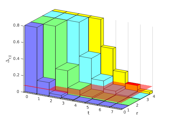
We can see the relation between (IP), (D), the allocated resource and the expected rank functions all together in Fig. 3. In the figure, the width for each $r$ in the $r$-axis is $h_{r}$, while the width for each $t$ is $1$. The height of the bar located at $(r,t)$ is $\Delta_{r,t}$, which is monotonic decreasing when $t$ increases. The red semitransparent surface acts as a “water surface”, where its height is the Lagrange multiplier.

The cross-section of Fig. 3 by fixing an $r$ is the one illustrated in Fig. 1 (after shifting the $t$-axis to the left so that the top of each bar lays between two integers). That is, in the view of Fig. 3, $t_{r}(\lambda)$ corresponds to the shortest bar of the corresponding $r$ which is above the water surface. If the water surface touches the top of the shortest bar, e.g., the solid red top face located at $(4,6)$, then the corresponding $t_{r}$ can be a non-integer.

We can illustrate the allocated resource from Fig. 3, which is the top view of Fig. 3. For each $r$, the sum of the areas of the top faces, i.e., the sum of the areas of the rectangles of the same color strip which are not covered in red in Fig. 3, is $h_{r}t_{r}$. The solid red face is an exception in a way that only a portion of the area is counted as this face corresponds to a non-integer $t_{r}$. In other words, the sum of the areas of the rectangles which are not covered in red in Fig. 3, plus a portion of the area of the solid red face, is the allocated resource.

Note that from the definition of $\Delta_{r,t}$, we can express $E_{r}(t_{r})$ by

Therefore, the objective value of (IP), $\sum_{r=0}^{M}h_{r}E_{r}(t_{r})$, is the sum of the volumes of the bars contributed to the areas for allocated resource, i.e., the volume of those bars which are taller than the water surface. Again, only a portion of the volume of bar with the solid red top face is counted.

From Fig. 3, we can also explain why our Algorithm 1 works. Suppose we start with a certain height of the water surface. The bars above the water surface gives an interior point as the starting point of the algorithm. We can set a water surface higher than the tallest bar so that we start from $t_{r}=0$ for all $r\in[M]$. We lower the water surface in each iteration until a new top face comes out from the water. This top face belongs to the tallest bar compared with those bars under the water. The height of this bar equals the largest $\Delta_{r,t_{r}}$ at this moment. When we lower the water surface to a point where the allocated resource (the area viewed from the top view) equals the total resource, then the algorithm stops. A special handling of the solid red face is done to calculate the portion of its area and volume to be included in the allocated resource and the objective respectively. This way, we can ensure that only those tallest bars are out of the water surface, thus the sum of volumes is maximized.

To further investigate the characteristic of the solution, e.g., the error toleration on the input rank distribution, and the behavior of the algorithms, e.g., starting from an arbitrary interior point which does not follow the water surface criteria, we present a useful representation of an optimal solution of (IP) and also an arbitrary interior point.

For any $r\in[M]$, define a function $\Omega_{r}$ which maps a non-negative real number to a multiset:

For simplicity, define $\Omega_{r}(\infty):=\{\Delta_{r,t}\colon t\in\mathbb{N}\}$. We use the notation $\uplus$ to represent the additive union of multisets [64].

Due to the property that $\Delta_{r,t}\geq\Delta_{r,t+1}$, every element in $\Omega_{r}(\infty)\setminus\Omega_{r}(t_{r})$ is no larger than the elements in $\Omega_{r}(t_{r})$ when $\Omega_{r}(t_{r})\neq\emptyset$. That is, we have $\min\Omega_{r}(t_{r})=\Delta_{r,\lceil t_{r}-1\rceil}$ when $t_{r}>0$. Also, the largest $\lceil t_{r}\rceil$ elements in $\Omega_{r}(\infty)$, which is exactly $\Omega_{r}(t_{r})$, can be used to represent the terms involved in (9). These properties can be easily seen in the $3$-D illustration in Fig. 3.

Now, we use a table of cells as shown in Fig. 4 to illustrate the above mathematical structures. The table reassembles the top view in Fig. 3 by neglecting the widths of the bars in the $r$-axis. This way, we can also visualize those $r$ where $h_{r}=0$. Each cell in Fig. 4 corresponds to a value of $\Delta_{r,t}$. The lower $\lceil t_{r}\rceil$ cells in column $r$ are all the elements in $\Omega_{r}(t_{r})$. In other words, $\Omega_{r}(\infty)$ can be represented by all the cells in column $r$.

We can use this relation to express $E_{r}(t_{r})$ in the table. For example, $E_{5}(8)$ is the sum of the lower $8$ cells in column $5$. When $t_{r}$ is not an integer, we can represent the fractional part by taking a part of a cell. For example, $E_{3}(4.5)$ is the sum of the lower $4$ cells plus half of the $5$-th cell in column $3$. The lower $\lceil 4.5\rceil=5$ cells in the column are involved in expressing $E_{3}(4.5)$.

If there is some $r$ where $h_{r}=0$, an arbitrary $t_{r}$ would not consume any resource nor affect the objective value in (IP). If the zero mass is due to certain error in measurement, we may receive a batch of rank $r$ and we need to make a reasonable decision on its recoding number. We defer the discussion of this case to the next subsection. In the remainder of this subsection, we concern those $r$ where $h_{r}\neq 0$.

References

- [1] H. H. F. Yin, B. Tang, K. H. Ng, S. Yang, X. Wang, and Q. Zhou, “A unified adaptive recoding framework for batched network coding,” in Proc. ISIT ’19, Jul. 2019, pp. 1962–1966.
- [2] T. Ho, R. Koetter, M. Médard, D. R. Karger, and M. Effros, “The benefits of coding over routing in a randomized setting,” in Proc. ISIT ’03, Jun. 2003, p. 442.
- [3] T. Ho, M. Médard, R. Koetter, D. R. Karger, M. Effros, J. Shi, and B. Leong, “A random linear network coding approach to multicast,” IEEE Trans. Inform. Theory, vol. 52, no. 10, pp. 4413–4430, Oct. 2006.
- [4] S. Jaggi, P. A. Chou, and K. Jain, “Low complexity optimal algebraic multicast codes,” in Proc. ISIT ’03, Jun. 2003, p. 368.
- [5] P. Sanders, S. Egner, and L. Tolhuizen, “Polynomial time algorithms for network information flow,” in Proc. SPAA ’03, Jun. 2003, pp. 286–294.
- [6] R. Ahlswede, N. Cai, S.-Y. R. Li, and R. W. Yeung, “Network information flow,” IEEE Trans. Inform. Theory, vol. 46, no. 4, pp. 1204–1216, Jul. 2000.
- [7] R. Koetter and M. Médard, “An algebraic approach to network coding,” IEEE/ACM Trans. Netw., vol. 11, no. 5, pp. 782–795, Oct. 2003.
- [8] S.-Y. R. Li, R. W. Yeung, and N. Cai, “Linear network coding,” IEEE Trans. Inform. Theory, vol. 49, no. 2, pp. 371–381, Feb. 2003.
- [9] Y. Wu, “A trellis connectivity analysis of random linear network coding with buffering,” in Proc. ISIT ’06, Jul. 2006, pp. 768–772.
- [10] D. S. Lun, M. Médard, R. Koetter, and M. Effros, “On coding for reliable communication over packet networks,” Physical Communication, vol. 1, no. 1, pp. 3–20, 2008.
- [11] P. A. Chou, Y. Wu, and K. Jain, “Practical network coding,” in Proc. Annual Allerton Conf. on Commun., Control and Comput., vol. 41, no. 1, Oct. 2003, pp. 40–49.
- [12] D. Silva, W. Zeng, and F. R. Kschischang, “Sparse network coding with overlapping classes,” in Proc. NetCod ’09, Jun. 2009, pp. 74–79.
- [13] A. Heidarzadeh and A. H. Banihashemi, “Overlapped chunked network coding,” in Proc. ITW ’10, Jan. 2010, pp. 1–5.
- [14] K. Mahdaviani, M. Ardakani, H. Bagheri, and C. Tellambura, “Gamma codes: A low-overhead linear-complexity network coding solution,” in Proc. NetCod ’12, Jun. 2012, pp. 125–130.
- [15] S. Yang and R. W. Yeung, “Batched sparse codes,” IEEE Trans. Inform. Theory, vol. 60, no. 9, pp. 5322–5346, Sep. 2014.
- [16] D. E. Lucani, M. V. Pedersen, D. Ruano, C. W. Sørensen, F. H. P. Fitzek, J. Heide, O. Geil, V. Nguyen, and M. Reisslein, “Fulcrum: Flexible network coding for heterogeneous devices,” IEEE Access, vol. 6, pp. 77 890–77 910, 2018.
- [17] V. Nguyen, E. Tasdemir, G. T. Nguyen, D. E. Lucani, F. H. P. Fitzek, and M. Reisslein, “Dsep fulcrum: Dynamic sparsity and expansion packets for fulcrum network coding,” IEEE Access, vol. 8, pp. 78 293–78 314, 2020.
- [18] Y. Li, E. Soljanin, and P. Spasojevic, “Effects of the generation size and overlap on throughput and complexity in randomized linear network coding,” IEEE Trans. Inform. Theory, vol. 57, no. 2, pp. 1111–1123, Feb. 2011.
- [19] B. Tang, S. Yang, Y. Yin, B. Ye, and S. Lu, “Expander chunked codes,” EURASIP Journal on Advances in Signal Processing, vol. 2015, no. 1, pp. 1–13, 2015. [Online]. Available: http://dx.doi.org/10.1186/s13634-015-0297-8
- [20] K. Mahdaviani, R. Yazdani, and M. Ardakani, “Overhead-optimized gamma network codes,” in Proc. NetCod ’13, 2013.
- [21] B. Tang and S. Yang, “An LDPC approach for chunked network codes,” IEEE/ACM Transactions on Networking, no. 1, pp. 605–617, Feb. 2018.
- [22] S. Yang, S.-W. Ho, J. Meng, and E.-H. Yang, “Capacity analysis of linear operator channels over finite fields,” IEEE Trans. Inform. Theory, vol. 60, no. 8, pp. 4880–4901, Aug. 2014.
- [23] Q. Zhou, S. Yang, H. H. F. Yin, and B. Tang, “On BATS codes with variable batch sizes,” IEEE Commun. Lett., vol. 21, no. 9, pp. 1917–1920, Sep. 2017.
- [24] Q. Huang, K. Sun, X. Li, and D. O. Wu, “Just FUN: A joint fountain coding and network coding approach to loss-tolerant information spreading,” in Proc. MobiHoc ’14, Aug. 2014, pp. 83–92.
- [25] H. F. H. Yin, S. Yang, and W.-H. R. Yeung, “Loss-resilient protocols for communication networks,” U.S. Patent 10 425 192, Sep. 24, 2019.
- [26] Z. Zhou, C. Li, S. Yang, and X. Guang, “Practical inner codes for BATS codes in multi-hop wireless networks,” IEEE Trans. Veh. Technol., vol. 68, no. 3, pp. 2751–2762, Mar. 2019.
- [27] Z. Zhou, J. Kang, and L. Zhou, “Joint BATS code and periodic scheduling in multihop wireless networks,” IEEE Access, vol. 8, pp. 29 690–29 701, Feb. 2020.
- [28] H. H. F. Yin, K. H. Ng, X. Wang, and Q. Cao, “On the minimum delay of block interleaver for batched network codes,” in Proc. ISIT ’19, Jul. 2019, pp. 1957–1961.
- [29] H. H. F. Yin, K. H. Ng, X. Wang, Q. Cao, and L. K. L. Ng, “On the memory requirements of block interleaver for batched network codes,” in Proc. ISIT ’20, Jun. 2020, pp. 1658–1663.
- [30] S. Yang, R. W. Yeung, J. H. F. Cheung, and H. H. F. Yin, “BATS: Network coding in action,” in Proc. Annual Allerton Conf. on Commun., Control, and Comput., Sep. 2014, pp. 1204–1211.
- [31] P. Maymounkov, N. J. A. Harvey, and D. S. Lun, “Methods for efficient network coding,” in Proc. Annual Allerton Conf. on Commun., Control and Comput., Sep. 2006, pp. 482–491.
- [32] B. Tang, S. Yang, B. Ye, S. Guo, and S. Lu, “Near-optimal one-sided scheduling for coded segmented network coding,” IEEE Trans. Comput., vol. 65, no. 3, pp. 929–939, Mar. 2016.
- [33] H. H. F. Yin, S. Yang, Q. Zhou, and L. M. L. Yung, “Adaptive recoding for BATS codes,” in Proc. ISIT ’16, Jul. 2016, pp. 2349–2353.
- [34] J. Wang, Z. Jia, H. H. F. Yin, and S. Yang, “Small-sample inferred adaptive recoding for batched network coding,” in Proc. ISIT ’21, Jul. 2021.
- [35] H. H. F. Yin and K. H. Ng, “Impact of packet loss rate estimation on blockwise adaptive recoding for batched network coding,” in Proc. ISIT ’21, Jul. 2021.
- [36] H. H. F. Yin, K. H. Ng, A. Z. Zhong, R. W. Yeung, and S. Yang, “Intrablock interleaving for batched network coding with blockwise adaptive recoding,” in Proc. ISIT ’21, Jul. 2021.
- [37] X. Xu, Y. L. Guan, and Y. Zeng, “Batched network coding with adaptive recoding for multi-hop erasure channels with memory,” IEEE Trans. Commun., vol. 66, no. 3, pp. 1042–1052, Mar. 2018.
- [38] H. H. F. Yin, X. Xu, K. H. Ng, Y. L. Guan, and R. W. Yeung, “Packet efficiency of BATS coding on wireless relay network with overhearing,” in Proc. ISIT ’19, Jul. 2019, pp. 1967–1971.
- [39] C. Zhang, B. Tang, B. Ye, and S. Lu, “An efficient chunked network code based transmission scheme in wireless networks,” in Proc. ICC ’17, May 2017, pp. 1–6.
- [40] E. N. Gilbert, “Capacity of a burst-noise channel,” Bell System Technical Journal, vol. 39, pp. 1253–1265, Sep. 1960.
- [41] E. O. Elliott, “Estimates of error rates for codes on burst-noise channels,” Bell System Technical Journal, vol. 42, pp. 1977–1997, Sep. 1963.
- [42] Y. Dong, S. Jin, S. Yang, and H. H. F. Yin, “Network utility maximization for BATS code enabled multihop wireless networks,” in Proc. ICC ’20, Jun. 2020.
- [43] H. H. F. Yin, R. W. Yeung, and S. Yang, “A protocol design paradigm for batched sparse codes,” Entropy, vol. 22, no. 7, Jul. 2020, Art. no. 790.
- [44] S. Yang and R. W. Yeung, BATS Codes: Theory and Practice, ser. Synthesis Lectures on Communication Networks. Morgan & Claypool Publishers, 2017.
- [45] A. Shokrollahi and M. Luby, Raptor Codes, ser. Foundations and Trends in Communications and Information Theory. now, 2011, vol. 6.
- [46] A. Shokrollahi, S. Lassen, and R. Karp, “Systems and processes for decoding chain reaction codes through inactivation,” U.S. Patent 6,856,263, Feb. 15, 2005.
- [47] J. A. Hartwell and A. O. Fapojuwo, “Modeling and characterization of frame loss process in IEEE 802.11 wireless local area networks,” in Proc. VTC ’04, vol. 6, Sep. 2004, pp. 4481–4485.
- [48] C. Tang and P. K. McKinley, “Modeling multicast packet losses in wireless LANs,” in Proc. MSWIM ’03, Sep. 2003, pp. 130–133.
- [49] J. Poikonen and J. Paavola, “Error models for the transport stream packet channel in the DVB-H link layer,” in Proc. ICC ’06, vol. 4, Jun. 2006, pp. 1861–1866.
- [50] S. Frohn, S. Gübner, and C. Lindemann, “Analyzing the effective throughput in multi-hop IEEE 802.11n networks,” Computer Communications, vol. 34, no. 16, pp. 1912–1921, Oct. 2011.
- [51] G. Haßlinger and O. Hohlfeld, “The Gilbert-Elliott model for packet loss in real time services on the internet,” in 14th GI/ITG Conference - Meas., Modelling and Evalutation of Comput. and Commun. Syst., Mar. 2008, pp. 1–15.
- [52] L. R. Rabiner, “A tutorial on hidden Markov models and selected applications in speech recognition,” Proc. IEEE, vol. 77, no. 2, pp. 257–286, Feb. 1989.
- [53] M. Yajnik, S. Moon, J. Kurose, and D. Towsley, “Measurement and modelling of the temporal dependence in packet loss,” in Conference on Computer Communications, vol. 1, Mar. 1999, pp. 345–352.
- [54] H. A. Sanneck and G. Carle, “Framework model for packet loss metrics based on loss runlengths,” in Multimedia Computing and Networking 2000, vol. 3969, Jan. 1999, pp. 177–187.
- [55] A. D. Clark, “Modeling the effects of burst packet loss and recency on subjective voice quality,” in Internet Telephony Workshop (IPtel 2001), Apr. 2001.
- [56] H. S. Wang and N. Moayeri, “Finite-state Markov channel – a useful model for radio communication channels,” IEEE Trans. Veh. Technol., vol. 44, no. 1, pp. 163–171, Feb. 1995.
- [57] J.-P. Ebert and A. Willig, “A Gilbert-Elliot bit error model and the efficient use in packet level simulation,” Technische Universität Berlin, Berlin, Tech. Rep. TKN-99-002, Mar. 1999.
- [58] J. Huang and L. Gao, Wireless Network Pricing. Morgan & Claypool Publishers, 2013.
- [59] S. Shakkottai and R. Srikant, “Network optimization and control,” Foundations and Trends in Networking, vol. 2, pp. 271–379, Jan. 2007.
- [60] F. P. Kelly, A. K. Maulloo, and D. K. H. Tan, “Rate control for communication networks: shadow prices, proportional fairness and stability,” JORS, vol. 49, no. 3, pp. 237–252, Mar. 1998.
- [61] S. H. Low and D. E. Lapsley, “Optimization flow control. I. basic algorithm and convergence,” IEEE/ACM Trans. Netw., vol. 7, no. 6, pp. 861–874, Dec. 1999.
- [62] O. Ardakanian, C. Rosenberg, and S. Keshav, “Distributed control of electric vehicle charging,” in Proc. e-Energy ’13, May 2013, pp. 101–112.
- [63] D. P. Palomar and M. Chiang, “A tutorial on decomposition methods for network utility maximization,” IEEE JSAC, vol. 24, no. 8, pp. 1439–1451, Aug. 2006.
- [64] W. D. Blizard, “Multiset theory,” Notre Dame J. Formal Logic, vol. 30, no. 1, pp. 36–66, Dec. 1988.
- [65] G. Landsberg, “Ueber eine anzahlbestimmung und eine damit zusammenhängende reihe,” Journal für die reine und angewandte Mathematik, vol. 111, pp. 87–88, 1893.
- [66] J. M. van Lint and R. M. Wilson, A Course in Combinatorics. Cambridge University Press, 1992.
- [67] V. F. Kolchin, Random Graphs. Cambridge University Press, 1999.
Appendix A Proof of Lemma 1
Let be the received packets in a batch. Without loss of generality, let be a basis of the vector space spanned by all the received packets in the batch. Then, we have
for all and some constants . A recoded packet generated by RLNC is a vector expressed by , where are chosen from uniformly, and
Let be random variables which are uniformly distributed over all entries in . For all where , we have . On the other hand, every row in the addition table of is a permutation of all the entries in . So, we have . The above arguments show that is distributed uniformly over . That is, the RLNC of all received packets is equivalent in distribution to the RLNC of all linearly independent received packets.
Let be the matrix formed by juxtaposing . The recoded packets are the columns in the matrix . Let be the matrix formed by juxtaposing the received recoded packets at the next hop. Note that , where the latter substitutes the lost packets into zero column vectors. So, we can express the expected rank function by
where the last equality holds as has full column rank.
Appendix B Proof of Lemma 2
Without loss of generality, we can write and , where and are independent totally random column vectors.
When , both and are empty matrices. By definition, their ranks are both . So, we have for all .
Now we consider . Denoted by the vector space spanned by the columns of a matrix . We have
where (B) holds since is a binary random variable. Similarly, we have
On the other hand,