跳到论文正文
W Papers独立论文阅读器 arXiv:2105.07536 论文正文 计算阅读时间 · 0%
引用这篇论文根据当前论文元数据生成,正式投稿前建议核对。


License: CC BY-NC-ND 4.0
arXiv:2105.07536v4 [stat.ML] 01 Nov 2022

Tony Cai and Rong Ma

Theoretical Foundations of t-SNE for Visualizing High-Dimensional Clustered Data

T. Tony Cai tcai@wharton.upenn.edu Affiliation: Department of Statistics and Data Science Affiliation: University of Pennsylvania Affiliation: Philadelphia, PA 19104, USA    Rong Ma rongm@stanford.edu Affiliation: Department of Statistics Affiliation: Stanford University Affiliation: Stanford, CA 94305, USA
Abstract

This paper investigates the theoretical foundations of the t-distributed stochastic neighbor embedding (t-SNE) algorithm, a popular nonlinear dimension reduction and data visualization method. A novel theoretical framework for the analysis of t-SNE based on the gradient descent approach is presented. For the early exaggeration stage of t-SNE, we show its asymptotic equivalence to power iterations based on the underlying graph Laplacian, characterize its limiting behavior, and uncover its deep connection to Laplacian spectral clustering, and fundamental principles including early stopping as implicit regularization. The results explain the intrinsic mechanism and the empirical benefits of such a computational strategy. For the embedding stage of t-SNE, we characterize the kinematics of the low-dimensional map throughout the iterations, and identify an amplification phase, featuring the intercluster repulsion and the expansive behavior of the low-dimensional map, and a stabilization phase. The general theory explains the fast convergence rate and the exceptional empirical performance of t-SNE for visualizing clustered data, brings forth the interpretations of the t-SNE visualizations, and provides theoretical guidance for applying t-SNE and selecting its tuning parameters in various applications.

††heading: 23 2022 1- 5/21; Revised 10/22 10/22 21-0524††shortheadings: Theoretical Foundation of t-SNE / Cai and Ma††firstpage: 1††editor: Ji Zhu
keywords
Clustering; Data visualization; Foundation of data science; Nonlinear dimension reduction; t-SNE

1 Introduction

Data visualization is critically important for understanding and interpreting the structure of large datasets, and has been recognized as one of the fundamental topics in data science (Donoho 2017). A collection of machine learning algorithms for data visualization and dimension reduction have been developed. Among them, the t-distributed stochastic neighbor embedding (t-SNE) algorithm, proposed by van der Maaten and Hinton 2008, is arguably one of the most popular methods and a state-of-art technique for a wide range of applications (Wang et al. 2021).

Specifically, t-SNE is an iterative algorithm for visualizing high-dimensional data by mapping the data points to a two- or finite-dimensional space. It creates a single map that reveals the intrinsic structures in a high-dimensional dataset, including trends, patterns, and outliers, through a nonlinear dimension reduction technique. In the past decade, the original t-SNE algorithm, along with its many variants (for example, Yang et al. 2009; Carreira-Perpinán 2010; Xie et al. 2011; van der Maaten 2014; Gisbrecht et al. 2015; Pezzotti et al. 2016; Im et al. 2018; Linderman et al. 2019; Chatzimparmpas et al. 2020), has made profound impact to the practice of scientific research, including genetics (Platzer 2013), molecular biology (Olivon et al. 2018), single-cell transcriptomics (Kobak and Berens 2019), computer vision (Cheng et al. 2015) and astrophysics (Traven et al. 2017). In particular, the extraordinary performance of t-SNE for visualizing high-dimensional data with intrinsic clusters has been widely acknowledged (van der Maaten 2014; Kobak and Berens 2019).

Compared to the extensive literature on the computational and numerical aspects of t-SNE, there is a paucity of fundamental results about its theoretical foundations (see Section 1.3 for a brief overview). The lack of theoretical understanding and justifications profoundly limits the users’ interpretation of the results as well as the potentials for further improvement of the method.

This paper aims to investigate the theoretical foundations of t-SNE. Specifically, we present a novel framework for the analysis of t-SNE, provide theoretical justifications for its competence in dimension reduction and visualizing clustered data, and uncover the fundamental principles underlying its exceptional empirical performance.

1.1 Basic t-SNE Algorithm

Let {Xi}1≤i≤n\{X_{i}\}_{1\leq i\leq n} be a set of pp-dimensional data points. t-SNE starts by computing a joint probability distribution over all pairs of data points {(Xi,Xj)}1≤i≠j≤n\{(X_{i},X_{j})\}_{1\leq i\neq j\leq n}, represented by a symmetric matrix ℙ=(pi​j)1≤i,j≤n∈ℝn×n\mathbb{P}=(p_{ij})_{1\leq i,j\leq n}\in\mathbb{R}^{n\times n}, where pi​i=0p_{ii}=0 for all 1≤i≤n1\leq i\leq n, and for i≠ji\neq j,

pi​j=pi|j+pj|i2​nwithpj|i=exp(−∥Xi−Xj∥22/2τi2)∑ℓ∈{1,2,…,n}∖{i}exp(−∥Xi−Xℓ∥22/2τi2).p_{ij}=\frac{p_{i|j}+p_{j|i}}{2n}\quad\text{with}\quad p_{j|i}=\frac{\exp(-\|X_{i}-X_{j}\|_{2}^{2}/2\tau_{i}^{2})}{\sum_{\ell\in\{1,2,...,n\}\setminus\{i\}}\exp(-\|X_{i}-X_{\ell}\|_{2}^{2}/2\tau_{i}^{2})}. (1)

Here τi\tau_{i} are tuning parameters, which are usually determined based on a certain perplexity measure and a binary search strategy (Hinton and Roweis 2002; van der Maaten and Hinton 2008). Similarly, for a two-dimensional11 1 Throughout, we focus on the two-dimensional embedding for ease of presentation. However, all the theoretical results obtained in this work holds for any finite constant embedding dimension. map {yi}1≤i≤n⊂ℝ2\{y_{i}\}_{1\leq i\leq n}\subset\mathbb{R}^{2}, we define the joint probability distribution over all pairs {(yi,yj)}1≤i≠j≤n\{(y_{i},y_{j})\}_{1\leq i\neq j\leq n} through a symmetric matrix ℚ=(qi​j)1≤i,j≤n\mathbb{Q}=(q_{ij})_{1\leq i,j\leq n} where qi​i=0q_{ii}=0 for all 1≤i≤n1\leq i\leq n and for i≠ji\neq j,

qi​j=(1+‖yi−yj‖22)−1∑ℓ,s∈{1,2,…,n},ℓ≠s(1+‖yℓ−ys‖22)−1.q_{ij}=\frac{(1+\|y_{i}-y_{j}\|_{2}^{2})^{-1}}{\sum_{\ell,s\in\{1,2,...,n\},\ell\neq s}(1+\|y_{\ell}-y_{s}\|_{2}^{2})^{-1}}. (2)

Intuitively, ℙ\mathbb{P} and ℚ\mathbb{Q} are similarity matrices summarizing the pairwise distances of the high-dimensional data points {Xi}1≤i≤n\{X_{i}\}_{1\leq i\leq n}, and the two-dimensional map {yi}1≤i≤n\{y_{i}\}_{1\leq i\leq n}, respectively. Then t-SNE aims to find {yi}1≤i≤n\{y_{i}\}_{1\leq i\leq n} that minimizes the KL-divergence between ℙ\mathbb{P} and ℚ\mathbb{Q}, that is,

(y1,…,yn)=arg​miny1,…,yn⁡DK​L​(ℙ,ℚ)=arg​miny1,…,yn⁡∑i,j∈{1,2,…,n}i≠jpi​j​log⁡pi​jqi​j.(y_{1},...,y_{n})=\mathop{\rm arg\min}_{y_{1},...,y_{n}}D_{KL}(\mathbb{P},\mathbb{Q})=\mathop{\rm arg\min}_{y_{1},...,y_{n}}\sum_{\begin{subarray}{c}i,j\in\{1,2,...,n\}\\ i\neq j\end{subarray}}p_{ij}\log\frac{p_{ij}}{q_{ij}}. (3)

Many algorithms have been proposed to solve this optimization problem. The most widely used algorithm was proposed in van der Maaten and Hinton 2008, which draws on a variant of gradient descent algorithm, with an updating equation

yi(k+1)=yi(k)+h​Di(k)+m(k+1)​(yi(k)−yi(k−1)),for i=1,…,n,y_{i}^{(k+1)}=y_{i}^{(k)}+hD_{i}^{(k)}+m^{(k+1)}(y_{i}^{(k)}-y_{i}^{(k-1)}),\quad\text{for $i=1,...,n,$} (4)

where h∈ℝ+h\in\mathbb{R}_{+} is a prespecified step size parameter, Di(k)=4​∑1≤j≤n,j≠i(yj(k)−yi(k))​Si​j(k)∈ℝ2D_{i}^{(k)}=4\sum_{1\leq j\leq n,j\neq i}(y^{(k)}_{j}-y^{(k)}_{i})S^{(k)}_{ij}\in\mathbb{R}^{2} is the gradient term corresponding to yiy_{i}, with Si​j(k)=(pi​j−qi​j(k))/(1+‖yi(k)−yj(k)‖22)∈ℝS^{(k)}_{ij}=(p_{ij}-q^{(k)}_{ij})/(1+\|y_{i}^{(k)}-y_{j}^{(k)}\|_{2}^{2})\in\mathbb{R}, and m(k)∈ℝ+m^{(k)}\in\mathbb{R}_{+} is a prespecified momentum parameter. The algorithm starts with an initialization yi(0)=yi(−1)y^{(0)}_{i}=y^{(-1)}_{i} for i∈{1,2,…,n}i\in\{1,2,...,n\}, drawn independently from a uniform distribution on [−0.01,0.01]2[-0.01,0.01]^{2}, or from N⁡(0,δ2​I)N(0,\delta^{2}I) for some small δ>0\delta>0.

As indicated by van der Maaten and Hinton 2008, the inclusion of the momentum term m(k+1)​(yi(k)−yi(k−1))m^{(k+1)}(y_{i}^{(k)}-y_{i}^{(k-1)}) in (4) is mainly to speed up the convergence and to reduce the risk of getting stuck in a local minimum. In this paper, for simplicity and generality we focus on the basic version of the t-SNE algorithm based on the simple gradient descent, with the updating equation

yi(k+1)=yi(k)+h​Di(k),for i=1,…,n.y_{i}^{(k+1)}=y_{i}^{(k)}+hD_{i}^{(k)},\quad\text{for $i=1,...,n.$} (5)

In van der Maaten and Hinton 2008 and van der Maaten 2014, the recommended total number of iterations is 1000, while the step size hh is initially set as 400 or 800, and is updated at each iteration by an adaptive learning rate scheme of Jacobs 1988.

The standard gradient descent algorithm as in (5) suffers from a slow convergence rate and even non-convergence in some applications. As an amelioration, van der Maaten and Hinton 2008 proposed an early exaggeration technique, applied to the initial stages of the optimization, that helps create patterns in the visualization and speed up the convergence. Such a computational strategy has been standard in practical use. In fact, most of the current software implementations of t-SNE are based on an early exaggeration stage followed by an embedding stage that iterates a certain gradient descent algorithm. In our setting, these two stages can be summarized as follows.

Early exaggeration stage.

For the first K0>0K_{0}>0 iterations, the pi​jp_{ij}’s in the gradient term Di(k)D_{i}^{(k)} are multiplied by some exaggeration parameter α>0\alpha>0, so the updating equation for this early exaggeration stage becomes

yi(k+1)=yi(k)+h∑1≤j≤n,j≠i(yj(k)−yi(k))Si​j(k)(α),i=1,…,n,y_{i}^{(k+1)}=y_{i}^{(k)}+h\sum_{1\leq j\leq n,j\neq i}(y^{(k)}_{j}-y^{(k)}_{i})S^{(k)}_{ij}(\alpha),\quad i=1,...,n, (6)

where Si​j(k)​(α)=(α​pi​j−qi​j(k))/(1+‖yi(k)−yj(k)‖22)∈ℝS^{(k)}_{ij}(\alpha)=(\alpha p_{ij}-q^{(k)}_{ij})/(1+\|y_{i}^{(k)}-y_{j}^{(k)}\|_{2}^{2})\in\mathbb{R}, and the factor 44 in Di(k)D_{i}^{(k)} is absorbed into the step size parameter hh. We refer to this first stage of the t-SNE algorithm as the early exaggeration stage.

In van der Maaten and Hinton 2008, the authors choose α=4\alpha=4 and K0=50K_{0}=50 for the early exaggeration stage, whereas later in van der Maaten 2014, it is recommended that α=12\alpha=12 and K0=250K_{0}=250. In particular, it is empirically observed that, the early exaggeration technique enables t-SNE to find a better global structure in the early stages of the optimization by creating very tight clusters of points that easily move around in the embedding space (van der Maaten 2014); this observation is later supported by some pioneering theoretical investigations (see Section 1.3). Nevertheless, there are interesting questions to be answered concerning (i) the underlying principles and mechanism behind such a computational strategy, (ii) the limit behavior of the low-dimensional map, (iii) how sensitive is the performance of t-SNE with respect to the choice of tuning parameters (α,h,K0)(\alpha,h,K_{0}), and (iv) how to efficiently determine these parameters to achieve the best empirical performance.

Refer to caption
Figure 1: An illustration of the t-SNE iterations that visualize samples from the MNIST dataset (Section 5). Each sample corresponds an image of handwritten digit “2,” “4,” “6,” or “8.” The visulaizations are obtained using the Rtsne function in the R package Rtsne, by selecting the exact t-SNE mode (theta=0, pca=F), dropping the momentum terms (momentum=0, final_momentum = 0), and setting perplexity=30 (default), α=12\alpha=12 (default), h=200h=200 (default) in (6), and K0=40K_{0}=40. The first three plots (top row) correspond to the early exaggeration stage, while the last three plots (bottom row) correspond to the embedding stage.

Embedding stage.

After the early exaggeration stage, the exaggeration parameter α\alpha is dropped and the original iterative algorithm (5) is carried out till attaining a prespecified number of steps. We refer to this second stage as the embedding stage. The final output is a two-dimensional map {yi(K1)}1≤i≤n\{y_{i}^{(K_{1})}\}_{1\leq i\leq n}, commonly treated as a low-dimensional embedding of the original data {Xi}1≤i≤n\{X_{i}\}_{1\leq i\leq n}, expected to preserve its intrinsic geometric structures.

In addition to data visualization, t-SNE is sometimes also used as an intermediate step for clustering, signal detection, among many other purposes. In particular, it has been observed that, when applied to high-dimensional clustered data, t-SNE tends to produce a visualization with more separated clusters, which are often in good agreement with the clusters found by a dedicated clustering algorithm (Kobak and Berens 2019). See Figure 1 for an example of data visualization using such a basic t-SNE algorithm.

1.2 Main Results and Our Contribution

A formal theoretical framework is introduced for the analysis of t-SNE that relies on a joint statistical and computational analysis. The key contribution of the present work can be summarized as follows:

  • •

    We rigorously establish the asymptotic equivalence between the early exaggeration stage and power iterations. Our theory unveils novel properties such as the implicit regularization effect and the necessity of early stopping in the early exaggeration stage for weakly clustered data.

  • •

    We characterize the behavior of t-SNE iterations at the embedding stage by identifying an amplification phase along with its intercluster repulsion and expansion phenomena, and a stabilization phase of this stage.

  • •

    We give the theoretical guidance for initialization and selecting the tuning parameters at both stages in a flexible and data-adaptive manner.

  • •

    We provide practical advice on applying t-SNE and interpreting the t-SNE visualizations of high-dimensional clustered data.

The main results can be explained in more detail from three perspectives.

Early exaggeration stage.

Through a discrete-time analysis (Sections 2.1 and 2.2), we establish the asymptotic equivalence between the early exaggeration stage and power iterations based on the underlying graph Laplacian associated with the high-dimensional data, providing a spectral-graphical interpretation of the algorithm. We show the implicit spectral clustering mechanism underlying this stage, which explains the adaptivity and flexibility of t-SNE for visualizing clustered data without specifying the number of clusters. Specifically, for the cases where {Xi}1≤i≤n\{X_{i}\}_{1\leq i\leq n} are approximately clustered into RR groups, we make the key observation that the coordinates of {yi(k)}1≤i≤n\{y^{(k)}_{i}\}_{1\leq i\leq n} converge to the RR-dimensional Laplacian null space, leading to a limiting embedding where the elements of {yi(k)}1≤i≤n\{y^{(k)}_{i}\}_{1\leq i\leq n} are well-clustered according to their true cluster membership. On the other hand, through a continuous-time analysis (Section 2.3), we study the underlying gradient flow and uncover an implicit regularization effect depending on the number of iterations. In particular, our analysis implies that when dealing with noisy and approximately clustered data, one should stop early in the early exaggeration stage to avoid “overshooting.” These results justify the empirical observations about the benefits of the early exaggeration technique in creating cluster structures and speeding up the algorithm. For more details about comparison with the existing results, see Section 1.3 and the discussions after Corollaries 7 in Section 2.

Embedding stage.

We provide a mechanical interpretation of the algorithm by characterizing the kinematics of the low-dimensional map at each iteration. Specifically, in Section 3 we identify an amplification phase within the embedding stage, featuring the local intercluster repulsion (Theorem 13) and the global expansive behavior (Theorem 15) of {yi(k)}1≤i≤n\{y_{i}^{(k)}\}_{1\leq i\leq n}. In the former case, it is shown that the movement of each yi(k)y_{i}^{(k)} to yi(k+1)y_{i}^{(k+1)} is jointly determined by the repulsive forces pointing toward yi(k)y_{i}^{(k)} from each of the other clusters (Figure 2), that amounts to increasing spaces between the existing clusters; in the latter case, it is shown the diameter of {yi(k)}1≤i≤n\{y_{i}^{(k)}\}_{1\leq i\leq n} may strictly increase after each iteration. We observe that, following the amplification phase, there is a stabilization phase where {yi(k)}1≤i≤n\{y_{i}^{(k)}\}_{1\leq i\leq n} is locally adjusted to achieve at a finer embedding of {Xi}1≤i≤n\{X_{i}\}_{1\leq i\leq n}. These results together explain the fast convergence rate and the exceptional empirical performance of t-SNE for visualizing clustered data. The articulation of these phenomena also leads to useful practical guidances. See below and Remark 16 in Section 3 for more details.

Refer to caption
Figure 2: Illustration of the intercluster repulsion where the original data {Xi}1≤i≤n\{X_{i}\}_{1\leq i\leq n} have three clusters. The position of yi(k+1)y_{i}^{(k+1)} is jointly determined by yi(k)y_{i}^{(k)} and two repulsive forces fi​1(k)f_{i1}^{(k)} and fi​2(k)f_{i2}^{(k)} pushing yi(k)y_{i}^{(k)} away from the other two clusters.

Practical implications.

The general theory brings forth the interpretations of the t-SNE output, and provides theoretical guidance for selecting tuning parameters and for initialization. In Section 4 we illustrate the general theory on two examples of high-dimensional clustered data, one generated from a Gaussian mixture model, and another from a noisy nested sphere model. We also analyze in Section 5 a real-world dataset to further demonstrate the practical implications of our theory. In particular, our analysis allows for a wider spectrum of tuning parameters (Figure 10 and Equation (39)) and initialization procedures than those considered in previous theoretical works (Arora et al. 2018; Linderman and Steinerberger 2019). Moreover, our theoretical results support the state-of-art practice (Kobak and Berens 2019; Kobak and Linderman 2021), but also lead to novel insights (e.g., the first item below) that has been unknown to our knowledge. In the following, we summarize our general advice on applying t-SNE to potentially clustered data:

  • •

    For weakly clustered data, one may adopt the early exaggeration technique, but needs to stop early (for example, set K0=⌊(log⁡n)2⌋K_{0}=\lfloor(\log n)^{2}\rfloor) to avoid overshooting – failure of stopping early may lead to false clustering; see Figure 5 below for an illustration.

  • •

    t-SNE visualization based on random initialization and early exaggeration is reliable in terms of cluster membership but not relative position of clusters. For example, the neighboring clusters in visualization may not be interpreted as neighboring clusters in the original data; see Figure 6 below for an illustration.

  • •

    Occasionally, false clustering may appear as an artifact of random initialization and intercluster repulsion. Therefore, it is helpful to run t-SNE multiple times to fully assess the effect of random initialization; see Figure 6 below for an illustration.

  • •

    For strongly clustered data, one can speed up the algorithm by replacing the early exaggeration stage by a simple spectral initialization22 2 An illustration is provided in Figure 4.1 of Linderman and Steinerberger 2019. where (𝒚1(0),𝒚2(0))(\boldsymbol{y}_{1}^{(0)},\boldsymbol{y}_{2}^{(0)}) are the eigenvectors associated with the smallest two eigenvalues of 𝕃⁡(ℙ)\mathbb{L}(\mathbb{P}).

1.3 Related Work

The impressive empirical performance of t-SNE has recently attracted much theoretical interests. Lee and Verleysen 2011 investigated the benefits of the so-called shift-invariant similarities used in the stochastic neighbor embedding and its variants. Later on, they further identified two key properties of these visualization methods (Lee and Verleysen 2014). In Shaham and Steinerberger 2017, a large family of methods including t-SNE as a special case were studied and shown to successfully map well-separated disjoint clusters from high dimensions to the real line so as to approximately preserve the clustering. In Arora et al. 2018, a theoretical framework was developed to formalize the notion of visualizing clustered data, which is used to analyze the early exaggeration stage of t-SNE, and to justify its high visualization quality. Linderman and Steinerberger 2019 showed that, in the early exaggeration stage of t-SNE, with properly chosen parameters α\alpha and hh, a subset of the two-dimensional map belonging to the same cluster will shrink in diameter, suggesting well-clustered visualization following iterations. We note that connections between the early exaggeration stage and power iterations have been pointed out in Arora et al. 2018 and Linderman and Steinerberger 2019, but the discussions therein are mostly informal and heuristic. In contrast, we provide rigorous theoretical justification for such a connection, identify its condition and explicate its consequences. By extending the idea of t-SNE, Im et al. 2018 considered a class of methods with various loss functions based on the ff-divergence, and theoretically assessed the performances of these methods based on a neighborhood-level precision-recall analysis. More recently, Zhang and Steinerberger 2021 proposed to view t-SNE as a force-based method which generates embeddings by balancing attractive and repulsive forces between data points. In particular, the limiting behavior of t-SNE was analyzed under a mean-field model where a single homogeneous cluster is present. At the empirical side, the recent works of Kobak and Berens 2019 and Kobak and Linderman 2021 summarize the state-of-art practice of using t-SNE to biological data. A comprehensive survey of existing data visualization methods and their properties can be found in Nonato and Aupetit 2018.

Despite these pioneering endeavors, the theoretical understanding of t-SNE is still limited. Many intriguing phenomena and important features that arise commonly in practice have not been well understood or properly explained. Moreover, it remains unclear how to properly interpret the t-SNE visualization and its potential artifacts. These important questions are carefully addressed in the current work for the case of clustered data. Compared to the existing works, the theoretical framework developed in our work leads to identification and explication of novel properties, phenomena, and important practical implications on t-SNE, as summarized at the beginning of Section 1.2.

1.4 Notation and Organization

For a vector 𝕒=(a1,…,an)⊤∈ℝn\mathbb{a}=(a_{1},...,a_{n})^{\top}\in\mathbb{R}^{n}, we denote diag​(a1,…,an)∈ℝn×n\text{diag}(a_{1},...,a_{n})\in\mathbb{R}^{n\times n} as the diagonal matrix whose ii-th diagonal entry is aia_{i}, and define the ℓp\ell_{p} norm ‖𝕒‖p=(∑i=1naip)1/p\|\mathbb{a}\|_{p}=\big(\sum_{i=1}^{n}a_{i}^{p}\big)^{1/p}. For a matrix 𝔸=(ai​j)∈ℝn×n\mathbb{A}=(a_{ij})\in\mathbb{R}^{n\times n}, we define its Frobenius norm as ‖𝔸‖F=∑i=1n∑j=1nai​j2\|\mathbb{A}\|_{F}=\sqrt{\sum_{i=1}^{n}\sum_{j=1}^{n}a^{2}_{ij}}, its ℓ∞\ell_{\infty}-norm as ‖𝔸‖∞=max1≤i,j≤n⁡|ai​j|\|\mathbb{A}\|_{\infty}=\max_{1\leq i,j\leq n}|a_{ij}|, and its spectral norm as ‖𝔸‖=sup‖𝕩‖2≤1‖𝔸​𝕩‖2\|\mathbb{A}\|=\sup_{\|\mathbb{x}\|_{2}\leq 1}\|\mathbb{A}\mathbb{x}\|_{2}; we also denote 𝔸.i∈ℝn\mathbb{A}_{.i}\in\mathbb{R}^{n} as its ii-th column and 𝔸i.∈ℝn\mathbb{A}_{i.}\in\mathbb{R}^{n} as its ii-th row. Let O⁡(n,k)={𝕍∈ℝn×k:𝕍⊤​𝕍=𝐈k}O(n,k)=\{\mathbb{V}\in\mathbb{R}^{n\times k}:\mathbb{V}^{\top}\mathbb{V}={\bf I}_{k}\} be the set of all n×kn\times k orthonormal matrices and On=O⁡(n,n)O_{n}=O(n,n), the set of nn-dimensional orthonormal matrices. For a rank rr matrix 𝔸∈ℝn×n\mathbb{A}\in\mathbb{R}^{n\times n} with 1≤r≤n1\leq r\leq n, its eigendecomposition is denoted as 𝔸=𝕌​Γ​𝕌⊤\mathbb{A}=\mathbb{U}\mathbb{\Gamma}\mathbb{U}^{\top} where 𝕌∈O⁡(n,r)\mathbb{U}\in O(n,r) with its columns being the eigenvectors, and Γ=diag​(λ1​(𝔸),λ2​(𝔸),…,λr​(𝔸))\mathbb{\Gamma}=\text{diag}(\lambda_{1}(\mathbb{A}),\lambda_{2}(\mathbb{A}),...,\lambda_{r}(\mathbb{A})) with λmin​(𝔸)=λ1​(𝔸)≤…≤λn​(𝔸)=λmax​(𝔸)\lambda_{\min}(\mathbb{A})=\lambda_{1}(\mathbb{A})\leq...\leq\lambda_{n}(\mathbb{A})=\lambda_{\max}(\mathbb{A}) being the ordered eigenvalues of 𝔸\mathbb{A}. For a smooth function f⁡(x)f(x), we denote f˙​(x)=d​f​(x)/d​x\dot{f}(x)=df(x)/dx and f¨​(x)=d2​f​(x)/d​x2\ddot{f}(x)=d^{2}f(x)/dx^{2}. For any integer n>0n>0, we denote the set [n]={1,2,…,n}[n]=\{1,2,...,n\}. For a finite set SS, we denote its cardinality as |S||S|. For a subset S⊆ℝnS\subseteq\mathbb{R}^{n}, we define its diameter diam​(S)=supx,y∈S‖x−y‖2\text{diam}(S)=\sup_{x,y\in S}\|x-y\|_{2}. For sequences {an}\{a_{n}\} and {bn}\{b_{n}\}, we write an=o⁡(bn)a_{n}=o(b_{n}) or an≪bna_{n}\ll b_{n} if limnan/bn=0\lim_{n}a_{n}/b_{n}=0, and write an=O⁡(bn)a_{n}=O(b_{n}), an≲bna_{n}\lesssim b_{n} or bn≳anb_{n}\gtrsim a_{n} if there exists a constant CC such that an≤C​bna_{n}\leq Cb_{n} for all nn. We write an≍bna_{n}\asymp b_{n} if an≲bna_{n}\lesssim b_{n} and an≳bna_{n}\gtrsim b_{n}. Throughout, C,C1,C2,…C,C_{1},C_{2},... are universal constants, that can vary from line to line.

The rest of the paper is organized as follows. Section 2 presents the theoretical analysis for the early exaggeration stage of t-SNE. Section 3 analyzes the embedding stage. The general theory is then applied in Section 4 to two specific settings of model-based clustered data, one under a Gaussian mixture model and another under a noisy nested sphere model. Analysis of a real-world dataset is presented in Section 5. Section 6 discusses potential applications, extensions and other related problems. Proofs of our main results and supplementary figures are collected in Appendix A to F.

2 Analysis of the Early Exaggeration Stage

2.1 Asymptotic Graphical Interpretation and Localization

We start with a key observation that connects the updating equation (6) to some graph-related concepts. To this end, we introduce the following definition.

Definition 1 (Degree & Laplacian Operators).

For a symmetric matrix 𝐀=(ai​j)1≤i,j≤n∈ℝn×n{\bf A}=(a_{ij})_{1\leq i,j\leq n}\in\mathbb{R}^{n\times n}, define the degree operator 𝔻:ℝn×n→ℝn×n\mathbb{D}:\mathbb{R}^{n\times n}\to\mathbb{R}^{n\times n} by 𝔻⁡(𝐀)=diag​(∑i=1nai​1,…,∑i=1nai​n)\mathbb{D}({\bf A})=\textup{diag}(\sum_{i=1}^{n}a_{i1},...,\sum_{i=1}^{n}a_{in}), and the Laplacian operator 𝕃:ℝn×n→ℝn×n\mathbb{L}:\mathbb{R}^{n\times n}\to\mathbb{R}^{n\times n} by 𝕃⁡(𝐀)=𝔻⁡(𝐀)−𝐀\mathbb{L}({\bf A})=\mathbb{D}({\bf A})-{\bf A}.

We define 𝕊α(k)=(Si​j(k)​(α))1≤i,j≤n∈ℝn×n\mathbb{S}^{(k)}_{\alpha}=(S^{(k)}_{ij}(\alpha))_{1\leq i,j\leq n}\in\mathbb{R}^{n\times n} with Si​i(k)​(α)≡0S^{(k)}_{ii}(\alpha)\equiv 0 for all i∈[n]i\in[n]. Then we can rewrite the updating equation (6) using the matrix form as

𝒚ℓ(k+1)=[𝐈n−h𝕃(𝕊α(k))]𝒚ℓ(k),ℓ=1,2,\boldsymbol{y}_{\ell}^{(k+1)}=[{\bf I}_{n}-h\mathbb{L}(\mathbb{S}^{(k)}_{\alpha})]\boldsymbol{y}_{\ell}^{(k)},\quad\ell=1,2, (7)

where 𝐈n∈ℝn×n{\bf I}_{n}\in\mathbb{R}^{n\times n} is the identity matrix, and 𝒚ℓ(k)∈ℝn\boldsymbol{y}^{(k)}_{\ell}\in\mathbb{R}^{n} consists of the ℓ\ell-th coordinates of {yi(k)}1≤i≤n\{y_{i}^{(k)}\}_{1\leq i\leq n}. As a consequence, for each iteration kk, if we treat the symmetric matrix 𝕊α(k)\mathbb{S}_{\alpha}^{(k)} as the adjacency matrix of a weighted graph G(k)G^{(k)} with nn nodes that summarizes the pairwise relationships between nn data points {Xi}1≤i≤n\{X_{i}\}_{1\leq i\leq n}, Equation (7) has an interpretation that links to the Laplacian matrix of such a weighted graph.

To better understand the meaning and the properties of the underlying graph G(k)G^{(k)} that evolve over iterations, we take a closer look at its adjacency matrix 𝕊α(k)\mathbb{S}_{\alpha}^{(k)}. In particular, one should keep in mind that in common applications of t-SNE, the early exaggeration stage has the following empirical features: (i) moderate or relatively large values of the exaggeration parameter α\alpha (default 12 in the R package Rtsne), (ii) local initializations {yi(0)}1≤i≤n\{y_{i}^{(0)}\}_{1\leq i\leq n} around the origin (see Section 1.1), and (iii) relative small diameters diam​({yi(k)}1≤i≤n)\text{diam}(\{y_{i}^{(k)}\}_{1\leq i\leq n}) over the iterations (Figure 1).

Our next result shows that, these empirical features of t-SNE have deep connections to the asymptotic behavior of the evolving underlying graphs and their adjacency matrices {𝕊α(k)}k≥1\{\mathbb{S}_{\alpha}^{(k)}\}_{k\geq 1} in the large sample limit (as n→∞n\to\infty).

Theorem 2 (Asymptotic Graphical Interpretation).

Recall that ℙ=(pi​j)1≤i,j≤n\mathbb{P}=(p_{ij})_{1\leq i,j\leq n} is defined in (1) and denote η(k)=[diam​({yi(k)}1≤i≤n)]2\eta^{(k)}=[\textup{diam}(\{y_{i}^{(k)}\}_{1\leq i\leq n})]^{2}. Then for any i,j∈[n]i,j\in[n] with i≠ji\neq j, and each k≥1k\geq 1 such that η(k)<1\eta^{(k)}<1, we have

|Si​j(k)​(α)−α​pi​j+1n⁡(n−1)|≤α​pi​j​η(k)+2​η(k)n⁡(n−1)​(1−η(k)).{\bigg|S_{ij}^{(k)}(\alpha)-{\alpha p_{ij}}+\frac{1}{n(n-1)}\bigg|}\leq\alpha p_{ij}\eta^{(k)}+\frac{2\eta^{(k)}}{n(n-1)(1-\eta^{(k)})}. (8)

Consequently, if we denote 𝟏n=(1,…,1)⊤∈ℝn{\bf 1}_{n}=(1,...,1)^{\top}\in\mathbb{R}^{n}, and ℍn=1n⁡(n−1)​(𝟏n​𝟏n⊤−𝐈n)\mathbb{H}_{n}=\frac{1}{n(n-1)}({\bf 1}_{n}{\bf 1}_{n}^{\top}-{\bf I}_{n}), then for each k≥1k\geq 1, as long as (η(k),α)(\eta^{(k)},\alpha) satisfies

η(k)≪‖ℙ‖n​‖ℙ‖∞,α≫1n​‖ℙ‖,as n→∞,\eta^{(k)}\ll{\frac{\|\mathbb{P}\|}{n\|\mathbb{P}\|_{\infty}}},\quad\alpha\gg\frac{1}{n\|\mathbb{P}\|},\quad\text{as $n\to\infty$,} (9)

we have

limn→∞‖𝕊α(k)−(α​ℙ−ℍn)‖‖α​ℙ−ℍn‖=0.\lim_{n\to\infty}\frac{\|\mathbb{S}_{\alpha}^{(k)}-(\alpha\mathbb{P}-\mathbb{H}_{n})\|}{\|\alpha\mathbb{P}-\mathbb{H}_{n}\|}=0. (10)

The above theorem implies that, for large nn, as long as the diameter of {yi(k)}1≤i≤n\{y_{i}^{(k)}\}_{1\leq i\leq n} remains sufficiently small and the exaggeration parameter α\alpha sufficiently large, the adjacency matrix 𝕊α(k)\mathbb{S}_{\alpha}^{(k)} behaves almost like a fixed matrix α​ℙ−ℍn\alpha\mathbb{P}-\mathbb{H}_{n} across the iterations. In other words, we may treat the updating equation (7) as an approximately linear equation

𝒚ℓ(k+1)≈[𝐈n−h𝕃(αℙ−ℍn)]𝒚ℓ(k),ℓ=1,2,\boldsymbol{y}_{\ell}^{(k+1)}\approx[{\bf I}_{n}-h\mathbb{L}(\alpha\mathbb{P}-\mathbb{H}_{n})]\boldsymbol{y}_{\ell}^{(k)},\quad\ell=1,2, (11)

where the linear operator 𝐈n−h​𝕃​(α​ℙ−ℍn){\bf I}_{n}-h\mathbb{L}(\alpha\mathbb{P}-\mathbb{H}_{n}) only relies on the Laplacian of a fixed weighted graph whose adjacency matrix is given by the scaled and shifted similarity matrix α​ℙ−ℍn\alpha\mathbb{P}-\mathbb{H}_{n}. This essentially opens the door to our key result on the asymptotic equivalence between the early exaggeration stage and power iterations.

Before we formally present such a result, we need to first point out an important phenomenon concerning the global behavior of the low-dimensional map at the early exaggeration stage. Specifically, we make the following assumptions on the initialization and the tuning parameters (α,h,k)(\alpha,h,k):

(I1) {yi(0)}1≤i≤n\{y_{i}^{(0)}\}_{1\leq i\leq n} satisfies minℓ∈[2]⁡‖𝒚ℓ(0)‖2>0\min_{\ell\in[2]}\|\boldsymbol{y}_{\ell}^{(0)}\|_{2}>0, and maxℓ∈[2]⁡‖𝒚ℓ(0)‖∞=O⁡(1)\max_{\ell\in[2]}\|\boldsymbol{y}_{\ell}^{(0)}\|_{\infty}=O(1) as n→∞n\to\infty; and (T1) the parameters (α,h,k)(\alpha,h,k) satisfy k⁡(n​h​α​‖ℙ‖∞+h/n)=O⁡(1)k(nh\alpha\|\mathbb{P}\|_{\infty}+h/n)=O(1) as n→∞n\to\infty.

Intuitively, Condition (I1) says that the initialization {yi(0)}1≤i≤n\{y_{i}^{(0)}\}_{1\leq i\leq n} should not be simply all zeros or unbounded, whereas the condition (T1) – as a consequence of (8) – essentially requires the cumulative deviations of h​𝕃​(𝕊α(k))h\mathbb{L}(\mathbb{S}_{\alpha}^{(k)}) from h​𝕃​(α​ℙ−ℍn)h\mathbb{L}(\alpha\mathbb{P}-\mathbb{H}_{n}) to be bounded. Our next result shows that, under these assumptions, the diameter of {yi(k)}1≤i≤n\{y_{i}^{(k)}\}_{1\leq i\leq n} may not increase throughout the iterations, so the embedding remains localized within the initial range.

Proposition 3 (Localization).

Suppose (I1) and (T1) hold. We have

diam​({yi(k+1)}1≤i≤n)≤C​maxℓ∈[2]​‖𝒚ℓ(0)‖∞,\textup{diam}(\{y_{i}^{(k+1)}\}_{1\leq i\leq n})\leq C\max_{\ell\in[2]}\|\boldsymbol{y}_{\ell}^{(0)}\|_{\infty}, (12)

for some universal constant C>0C>0.

The above proposition confirmed the globally localized and non-expansive behavior of {yi(k)}1≤i≤n\{y_{i}^{(k)}\}_{1\leq i\leq n} over the early exaggeration stage observed in practice (Figure 1). Concerning Theorem 2, it tells us the step-specific condition η(k)≪‖ℙ‖/(n​‖ℙ‖∞)\eta^{(k)}\ll{\|\mathbb{P}\|}/(n\|\mathbb{P}\|_{\infty}) therein can be generalized to all finite kk’s as long as the initialization {yi(0)}1≤i≤n\{y_{i}^{(0)}\}_{1\leq i\leq n} is concentrated around 0, that is, maxℓ∈[2]⁡‖𝒚ℓ(0)‖∞2≪‖ℙ‖/(n​‖ℙ‖∞)\max_{\ell\in[2]}\|\boldsymbol{y}_{\ell}^{(0)}\|_{\infty}^{2}\ll\|\mathbb{P}\|/(n\|\mathbb{P}\|_{\infty}). Furthermore, when (α,h)(\alpha,h) are chosen such that the step-wise deviation diminishes (i.e., rn=n​h​α​‖ℙ‖∞+h/n→0r_{n}=nh\alpha\|\mathbb{P}\|_{\infty}+h/n\to 0), Proposition 3 indicates that (10) may remain true for even larger numbers of iterations as long as k=O⁡(rn−1)k=O(r_{n}^{-1}).

2.2 Asymptotic Power Iterations, Implicit Spectral Clustering and Early Stopping

With the above graphical interpretation of the updating equation (7) in mind, we now present our key result concerning the asymptotic equivalence between the early exaggeration stage and a power method based on the Laplacian matrix 𝕃⁡(α​ℙ−ℍn)\mathbb{L}(\alpha\mathbb{P}-\mathbb{H}_{n}). In particular, we make the following assumptions on the initialization and the tuning parameters:

(I2) {yi(0)}1≤i≤n\{y_{i}^{(0)}\}_{1\leq i\leq n} satisfies maxℓ∈[2]⁡‖𝒚ℓ(0)‖∞2=o⁡(‖ℙ‖/(n​‖ℙ‖∞))\max_{\ell\in[2]}\|\boldsymbol{y}_{\ell}^{(0)}\|_{\infty}^{2}=o(\|\mathbb{P}\|/(n\|\mathbb{P}\|_{\infty})) as n→∞n\to\infty; and (T1.D) The parameters (α,h,k)(\alpha,h,k) satisfy α≫(n​‖ℙ‖)−1\alpha\gg(n\|\mathbb{P}\|)^{-1} and k⁡(n​h​α​‖ℙ‖∞+h/n)=o⁡(1)k(nh\alpha\|\mathbb{P}\|_{\infty}+h/n)=o(1) as n→∞n\to\infty.

Condition (I2) follows from the discussion subsequent to Proposition 3, which along with Condition (T1.D), which is analogous to but stronger than (T1), ensures the conditions for Theorem 2 and Proposition 3 to hold simultaneously.

Theorem 4 (Asymptotic power iterations).

Under Conditions (I1) (I2) and (T1.D), we have (10) and (12) hold, and so does the asymptotic equivalence

limn→∞‖𝒚ℓ(k)−[𝐈n−h​𝕃​(α​ℙ−ℍn)]k​𝒚ℓ(0)‖2‖𝒚ℓ(0)‖2=0.\lim_{n\to\infty}\frac{\|\boldsymbol{y}_{\ell}^{(k)}-[{\bf I}_{n}-h\mathbb{L}(\alpha\mathbb{P}-\mathbb{H}_{n})]^{k}\boldsymbol{y}_{\ell}^{(0)}\|_{2}}{\|\boldsymbol{y}_{\ell}^{(0)}\|_{2}}=0. (13)

The above theorem suggests that each step of the early exaggeration stage may be treated as a power method in the sense that

𝒚ℓ(k+1)≈[𝐈n−h​𝕃​(α​ℙ−ℍn)]k​𝒚ℓ(0).\boldsymbol{y}_{\ell}^{(k+1)}\approx[{\bf I}_{n}-h\mathbb{L}(\alpha\mathbb{P}-\mathbb{H}_{n})]^{k}\boldsymbol{y}_{\ell}^{(0)}. (14)

The normalization by ‖𝒚ℓ(0)‖2\|\boldsymbol{y}_{\ell}^{(0)}\|_{2} in (13) makes sure the result to be scale-invariant to the initialization. It is well-known that, for a fixed matrix 𝔾∈ℝn×n\mathbb{G}\in\mathbb{R}^{n\times n} with 1 as its unique largest eigenvalue in magnitude, the power iteration 𝒚(k)=𝔾k​𝒚(0)\boldsymbol{y}^{(k)}=\mathbb{G}^{k}\boldsymbol{y}^{(0)} converges to the associated eigenvector as k→∞k\to\infty. As a result, when treated as an approximate power method, the early exaggeration stage of t-SNE essentially aims to find the direction of the leading eigenvector(s) of the matrix 𝐈n−h​𝕃​(α​ℙ−ℍn){\bf I}_{n}-h\mathbb{L}(\alpha\mathbb{P}-\mathbb{H}_{n}), which, as will be shown shortly, is actually equivalent to finding the eigenvector(s) associated with the smallest eigenvalue of the graph Laplacian 𝕃⁡(α​ℙ−ℍn)\mathbb{L}(\alpha\mathbb{P}-\mathbb{H}_{n}), or the null space of 𝕃⁡(ℙ)\mathbb{L}(\mathbb{P}).

Led by these observations, our next results concern the limiting behavior of the low-dimensional map {yi(k)}1≤i≤n\{y_{i}^{(k)}\}_{1\leq i\leq n} as the number of iterations k→∞k\to\infty. Note that any Laplacian matrix has an eigenvalue 00 associated with a trivial eigenvector n−1/2𝟏n^{-1/2}{\bf 1}. Given the affinity (14) between t-SNE and the power method, we start by showing that, the linear operator [𝐈n−h​𝕃​(α​ℙ−ℍn)]k[{\bf I}_{n}-h\mathbb{L}(\alpha\mathbb{P}-\mathbb{H}_{n})]^{k} would converge eventually to a projection operator associated with the null space of the Laplacian 𝕃⁡(ℙ)\mathbb{L}(\mathbb{P}). In particular, we let R≥1R\geq 1 be the dimension of the null space of the Laplacian 𝕃⁡(ℙ)∈ℝn×n\mathbb{L}(\mathbb{P})\in\mathbb{R}^{n\times n}; and assume

(T2) the parameters (α,h)(\alpha,h) satisfies κ<h​λR+1​(𝕃⁡(α​ℙ))≤h​λn​(𝕃⁡(α​ℙ))<1\kappa<h\lambda_{R+1}(\mathbb{L}(\alpha\mathbb{P}))\leq h\lambda_{n}(\mathbb{L}(\alpha\mathbb{P}))<1 for some constant κ∈(0,1)\kappa\in(0,1).

This assumption corresponds to the so-called “eigengap” condition in the random matrix literature, which gives the signal strength requirements for the recovery of the eigenvalues/eigenvectors, and, in the meantime, the conditions for the tuning parameters.

Theorem 5 (Convergence of power iterations).

Let 𝕌∈O⁡(n,R)\mathbb{U}\in O(n,R) such that its columns consist of an orthogonal basis for the null space of 𝕃⁡(ℙ)\mathbb{L}(\mathbb{P}). Suppose k​h=o⁡(n)kh=o(n) and (T2) hold. Then, we have

limk→∞‖[𝐈n−h​𝕃​(α​ℙ−ℍn)]k​𝒚−𝕌​𝕌⊤​𝒚‖2‖𝒚‖2=0.\lim_{k\to\infty}\frac{\|[{\bf I}_{n}-h\mathbb{L}(\alpha\mathbb{P}-\mathbb{H}_{n})]^{k}\boldsymbol{y}-\mathbb{U}\mathbb{U}^{\top}\boldsymbol{y}\|_{2}}{\|\boldsymbol{y}\|_{2}}=0. (15)

Combining Theorems 4 and 5, we know that for sufficiently large nn and kk, the t-SNE iterations 𝒚ℓ(k)\boldsymbol{y}_{\ell}^{(k)} may converge to the projection of the initial vectors 𝒚ℓ(0)\boldsymbol{y}_{\ell}^{(0)} into the null space of the Laplacian 𝕃⁡(ℙ)\mathbb{L}(\mathbb{P}), that is

𝒚ℓ(k)≈𝕌​𝕌⊤​𝒚ℓ(0),ℓ∈[2].\boldsymbol{y}_{\ell}^{(k)}\approx\mathbb{U}\mathbb{U}^{\top}\boldsymbol{y}_{\ell}^{(0)},\quad\ell\in[2]. (16)

Now, to better understand the above theorem and its implications on the limiting behavior of t-SNE applied to clustered data, we study the null space of a special class of Laplacian matrices, corresponding to the family of weighted graphs consisting of R≥2R\geq 2 connected components. In fact, when the original data {Xi}1≤i≤n\{X_{i}\}_{1\leq i\leq n} are well-clustered and τi\tau_{i}’s are appropriately chosen, the family of disconnected weighted graphs arise naturally since their adjacency matrices are good approximations of ℙ\mathbb{P} based on these data (Balakrishnan et al. 2011). We illustrate this point further in Section 4. In the following, we say a symmetric adjacency matrix ℙ\mathbb{P} is “well-conditioned” if its associated weighted graph has R≥2R\geq 2 connected components. Our next result characterizes the Laplacian null space corresponding to these disconnected weighted graphs.

Proposition 6 (Laplacian null space).

Suppose 𝔸∈ℝn×n\mathbb{A}\in\mathbb{R}^{n\times n} is symmetric and well conditioned. Then the smallest eigenvalue of the Laplacian 𝕃⁡(𝔸)\mathbb{L}(\mathbb{A}) is 00 and has multiplicity RR, and the associated eigen subspace is spanned by {𝛉1,…,𝛉R}\{\boldsymbol{\theta}_{1},...,\boldsymbol{\theta}_{R}\} where for each r∈{1,…,R}r\in\{1,...,R\},

[𝜽r]j={1/nrif the j-th node belongs to the r-th component0otherwise,[\boldsymbol{\theta}_{r}]_{j}=\left\{\begin{array}[]{ll}1/\sqrt{n_{r}}&\textrm{if the $j$-th node belongs to the $r$-th component}\\ 0&\textrm{otherwise}\end{array}\right.,

and nrn_{r} is the number of nodes in the rr-th connected component. In particular, up to possible permutation of coordinates, any vector 𝕦\mathbb{u} in the null space of 𝕃⁡(𝔸)\mathbb{L}(\mathbb{A}) can be expressed as

𝕦=a1n1​[𝟏n1𝟎𝟎]+a2n2​[𝟎𝟏n2𝟎]+…+aRnR​[𝟎𝟎𝟏nR],\mathbb{u}=\frac{a_{1}}{\sqrt{n_{1}}}\begin{bmatrix}{\bf 1}_{n_{1}}\\ {\bf 0}\\ \vdots\\ {\bf 0}\end{bmatrix}+\frac{a_{2}}{\sqrt{n_{2}}}\begin{bmatrix}{\bf 0}\\ {\bf 1}_{n_{2}}\\ \vdots\\ {\bf 0}\end{bmatrix}+...+\frac{a_{R}}{\sqrt{n_{R}}}\begin{bmatrix}{\bf 0}\\ {\bf 0}\\ \vdots\\ {\bf 1}_{n_{R}}\end{bmatrix}, (17)

for some a1,…,aR∈ℝa_{1},...,a_{R}\in\mathbb{R}.

From the above proposition, for a well-conditioned matrix, the components of any 𝕦\mathbb{u} in the Laplacian null space has at most RR distinct values, and whenever |{a1,…,aR}|=R|\{a_{1},...,a_{R}\}|=R, the coordinates share the same value if and only if the corresponding nodes fall in the same connected component, i.e., the same cluster. Combining (16) and (17), one can see that, for strongly clustered data, the output from the early exaggeration stage essentially converges to the eigenvectors associated with the Laplacian null space. This leads to our fourth practical advice at the end of Section 1.2.

We now generalize the analysis to the setting where the data {Xi}1≤i≤n\{X_{i}\}_{1\leq i\leq n} is only weakly clustered in the sense that there exists a well-conditioned symmetric matrix ℙ∗\mathbb{P}^{*} close to ℙ\mathbb{P} under properly chosen {τi}\{\tau_{i}\}, and the underlying graph associated with ℙ\mathbb{P} may not be necessarily disconnected. More specifically, we assume

(T2.D) there exists a symmetric and well-conditioned matrix ℙ∗∈ℝn×n\mathbb{P}^{*}\in\mathbb{R}^{n\times n} satisfying (T2) and is sufficiently close to ℙ\mathbb{P} in the sense that k​h​α​‖𝕃⁡(ℙ∗−ℙ)‖=o⁡(1)kh\alpha\|\mathbb{L}(\mathbb{P}^{*}-\mathbb{P})\|=o(1).

For a given ℙ\mathbb{P} satisfying (T2.D), let nrn_{r} with r∈[R]r\in[R] be the size of the rr-th connected component in the graph associated with ℙ∗\mathbb{P}^{*}. Our next theorem obtains the implicit spectral clustering and early stopping properties of the early exaggeration stage.

Theorem 7 (Implicit clustering and early stopping).

Suppose the similarity ℙ\mathbb{P} and the tuning parameters (α,h,k)(\alpha,h,k) satisfy (T1.D) and (T2.D), and the initialization satisfies (I1) and (I2). Then there exists some permutation matrix O∈ℝn×nO\in\mathbb{R}^{n\times n} such that, for ℓ∈[2]\ell\in[2],

lim(k,n)→∞‖𝒚ℓ(k)−O​𝕫ℓ‖2‖𝒚ℓ(0)‖2=0,\lim_{(k,n)\to\infty}\frac{\|\boldsymbol{y}_{\ell}^{(k)}-O\mathbb{z}_{\ell}\|_{2}}{\|\boldsymbol{y}_{\ell}^{(0)}\|_{2}}=0, (18)

where

𝕫ℓ=(zℓ​1,…,zℓ​1⏟n1,zℓ​2,…,zℓ​2⏟n2,…,zℓ​R,…,zℓ​R⏟nR)⊤∈ℝn,\mathbb{z}_{\ell}=(\underbrace{z_{\ell 1},...,z_{\ell 1}}_{n_{1}},\underbrace{z_{\ell 2},...,z_{\ell 2}}_{n_{2}},...,\underbrace{z_{\ell R},...,z_{\ell R}}_{n_{R}})^{\top}\in\mathbb{R}^{n}, (19)

and zℓ​r=𝛉r⊤​𝐲ℓ(0)/nrz_{\ell r}=\boldsymbol{\theta}_{r}^{\top}\boldsymbol{y}_{\ell}^{(0)}/\sqrt{n_{r}} for r∈[R]r\in[R].

Theorem 7 describes the limiting behavior of the low-dimensional map {yi(k)}1≤i≤n\{y_{i}^{(k)}\}_{1\leq i\leq n} as (n,k)→∞(n,k)\to\infty, when the original data is approximately clustered. Specifically, elements from {yi(k)}1≤i≤n\{y_{i}^{(k)}\}_{1\leq i\leq n} associated with a connected component of the underlying graph would converge cluster-wise towards a few points on ℝ2\mathbb{R}^{2}. In particular, Theorem 7 suggests that, at the end of the early exaggeration stage, although the samples belonging to the same underlying cluster tend to be clustered together in the t-SNE embeddings, the cluster centers of the t-SNE embeddings only rely on the initialization, rather than the actual positions of the underlying clusters. Therefore, if initialized randomly and noninformatively, the t-SNE embeddings at the end of the early exaggeration stage tend to preserve only the local structures (i.e., the closeness of the samples from the same cluster) but not the global structures (i.e., the relative positions of different clusters) of the original data (Kobak and Berens 2019; Kobak and Linderman 2021). This observation, as illustrated in Figure 6, leads to our second practical advice at the end of Section 1.2.

Our theory refines and improves the existing works such as Linderman and Steinerberger 2019 and Arora et al. 2018 in various aspects. Firstly, our theoretical framework formalizes and explains the asymptotic equivalence between the early exaggeration stage and the power iterations. The theory provides a precise description of the limiting behavior of the low-dimensional map and the theoretical conditions. Secondly, unlike the previous works where only one particular initialization and relatively limited range of tuning parameters were considered, our analysis yields general conditions and allows for more flexible choices of the initialization procedures and tuning parameters. Finally, our analysis unveils the need of stopping early in the early exaggeration stage for weakly clustered data, which is a novel feature. Specifically, both Conditions (T1.D) and (T2.D) allow k→∞k\to\infty but in a controlled manner – whenever ‖𝕃⁡(ℙ∗−ℙ)‖≠0\|\mathbb{L}(\mathbb{P}^{*}-\mathbb{P})\|\neq 0, there is a data dependent upper bound on the iteration number

k≪1h​α​‖𝕃⁡(ℙ∗−ℙ)‖,k\ll\frac{1}{h\alpha\|\mathbb{L}(\mathbb{P}^{*}-\mathbb{P})\|},

which becomes more stringent for weakly clustered data (i.e., ‖𝕃⁡(ℙ∗−ℙ)‖\|\mathbb{L}(\mathbb{P}^{*}-\mathbb{P})\| not too small). Such a phenomenon is also observed empirically (Figure 5), where failing to stop early would lead to false clustering.

2.3 Gradient Flow and Implicit Regularization

For ℓ∈{1,2}\ell\in\{1,2\}, let {𝒚~ℓ(k)}k≥0\{\tilde{\boldsymbol{y}}_{\ell}^{(k)}\}_{k\geq 0} be the sequence defined by the power iterations 𝒚~ℓ(k)=[𝐈n−h​𝕃​(α​ℙ−ℍn)]k​𝒚ℓ(0)\tilde{\boldsymbol{y}}_{\ell}^{(k)}=[{\bf I}_{n}-h\mathbb{L}(\alpha\mathbb{P}-\mathbb{H}_{n})]^{k}\boldsymbol{y}_{\ell}^{(0)}. Theorem 4 shows that {𝒚~ℓ(k)}k≥0\{\tilde{\boldsymbol{y}}_{\ell}^{(k)}\}_{k\geq 0} well approximates the t-SNE iterations {𝒚ℓ(k)}k≥0\{\boldsymbol{y}_{\ell}^{(k)}\}_{k\geq 0} in the large sample limit. The sequence {𝒚~ℓ(k)}k≥0\{\tilde{\boldsymbol{y}}_{\ell}^{(k)}\}_{k\geq 0} admits the updating equation

𝒚~ℓ(k+1)=𝒚~ℓ(k)−h​𝕃​(α​ℙ−ℍn)​𝒚~ℓ(k),k≥0,\tilde{\boldsymbol{y}}_{\ell}^{(k+1)}=\tilde{\boldsymbol{y}}_{\ell}^{(k)}-h\mathbb{L}(\alpha\mathbb{P}-\mathbb{H}_{n})\tilde{\boldsymbol{y}}_{\ell}^{(k)},\quad k\geq 0, (20)

with an initial value 𝒚~ℓ(0)=𝒚ℓ(0)\tilde{\boldsymbol{y}}_{\ell}^{(0)}={\boldsymbol{y}}_{\ell}^{(0)}. Treating Equation (20) as an auxiliary gradient descent algorithm to the original algorithm (7), a continuous-time analysis can be developed accordingly, which yields interesting insights about the t-SNE iterations {𝒚ℓ(k)}k≥0\{\boldsymbol{y}_{\ell}^{(k)}\}_{k\geq 0}.

We begin by modeling {𝒚~ℓ(k)}k≥0\{\tilde{\boldsymbol{y}}_{\ell}^{(k)}\}_{k\geq 0} by a smooth curve 𝕐ℓ​(t)\mathbb{Y}_{\ell}(t) with the Ansatz 𝒚~ℓ(k)≈𝕐ℓ​(k​h)\tilde{\boldsymbol{y}}_{\ell}^{(k)}\approx\mathbb{Y}_{\ell}(kh). Define a step function 𝒚ℓ,h​(t)=𝒚~ℓ(k)\boldsymbol{y}_{\ell,h}(t)=\tilde{\boldsymbol{y}}_{\ell}^{(k)} for k​h≤t<(k+1)​hkh\leq t<(k+1)h, and as h→0h\to 0, 𝒚ℓ,h​(t)\boldsymbol{y}_{\ell,h}(t) approaches 𝕐ℓ​(t)\mathbb{Y}_{\ell}(t) satisfying

𝕐˙ℓ​(t)=𝕃⁡(α​ℙ−ℍn)​𝕐ℓ​(t),\dot{\mathbb{Y}}_{\ell}(t)=\mathbb{L}(\alpha\mathbb{P}-\mathbb{H}_{n})\mathbb{Y}_{\ell}(t), (21)

with the initial value 𝕐ℓ​(0)=𝒚~ℓ(0)=𝒚ℓ(0)\mathbb{Y}_{\ell}(0)=\tilde{\boldsymbol{y}}_{\ell}^{(0)}={\boldsymbol{y}}_{\ell}^{(0)}. The above first-order differential equation (21) is usually referred as the gradient flow associated with the power iteration sequence {𝒚~ℓ(k)}k≥0\{\tilde{\boldsymbol{y}}_{\ell}^{(k)}\}_{k\geq 0}, whose limiting behavior can be studied through the step function 𝒚ℓ,h​(t)\boldsymbol{y}_{\ell,h}(t). The following theorem provides a non-asymptotic uniform upper bound on the deviation of 𝒚ℓ,h​(t)\boldsymbol{y}_{\ell,h}(t) from 𝕐⁡(t)\mathbb{Y}(t) over t∈[0,T]t\in[0,T] and that of 𝒚~ℓ(k)\tilde{\boldsymbol{y}}_{\ell}^{(k)} from 𝕐⁡(k​h)\mathbb{Y}(kh) over k≤T/hk\leq T/h.

Proposition 8 (Gradient flow).

For ℓ=1,2\ell=1,2, and any given T>0T>0, we have

supt∈[0,T]‖𝒚ℓ,h​(t)−𝕐ℓ​(t)‖2‖𝕐ℓ​(t)‖2≤T​h​‖𝕃⁡(α​ℙ−ℍn)‖2,\sup_{t\in[0,T]}\frac{\|{\boldsymbol{y}}_{\ell,h}(t)-\mathbb{Y}_{\ell}(t)\|_{2}}{\|\mathbb{Y}_{\ell}(t)\|_{2}}\leq Th\|\mathbb{L}(\alpha\mathbb{P}-\mathbb{H}_{n})\|^{2}, (22)

where 𝐲ℓ,h​(t)\boldsymbol{y}_{\ell,h}(t) is the continuous-time step process of {𝐲~ℓ(k)}\{\tilde{\boldsymbol{y}}_{\ell}^{(k)}\} generated by (20), and 𝕐ℓ​(t)\mathbb{Y}_{\ell}(t) is the solution to the ordinary differential equation (21). As a consequence, for t=h​kt=hk, if k​h2​‖𝕃⁡(α​ℙ−ℍn)‖2→0kh^{2}\|\mathbb{L}(\alpha\mathbb{P}-\mathbb{H}_{n})\|^{2}\to 0 as n→∞n\to\infty, then for ℓ∈{1,2}\ell\in\{1,2\},

lim(n,k)→∞‖𝒚~ℓ(k)−𝕐ℓ​(h​k)‖2‖𝒚ℓ(0)‖2=0.\lim_{(n,k)\to\infty}\frac{\|\tilde{\boldsymbol{y}}_{\ell}^{(k)}-\mathbb{Y}_{\ell}(hk)\|_{2}}{\|\boldsymbol{y}_{\ell}^{(0)}\|_{2}}=0. (23)

Combining Theorems 4 and 8, we obtain the approximation 𝒚ℓ(k)≈𝕐ℓ​(k​h)\boldsymbol{y}_{\ell}^{(k)}\approx\mathbb{Y}_{\ell}(kh) over a range of k≥0k\geq 0, for properly chosen parameters (α,h,k)(\alpha,h,k) and initialization. Consequently, the properties of the solution path 𝕐ℓ​(t)\mathbb{Y}_{\ell}(t) may provide important insights on the behavior of the t-SNE iterations at the early exaggeration stage. We start by stating the following proposition concerning the explicit expression of 𝕐ℓ​(t)\mathbb{Y}_{\ell}(t).

Proposition 9 (Solution path).

For ℓ∈{1,2}\ell\in\{1,2\}, the first-order linear differential equation (21) with initial value 𝕐ℓ​(0)=𝐲ℓ(0)\mathbb{Y}_{\ell}(0)=\boldsymbol{y}_{\ell}^{(0)} has the unique solution 𝕐ℓ​(t)=exp⁡(−t​𝕃​(α​ℙ−ℍn))​𝐲ℓ(0)\mathbb{Y}_{\ell}(t)=\exp(-t\mathbb{L}(\alpha\mathbb{P}-\mathbb{H}_{n}))\boldsymbol{y}_{\ell}^{(0)}, where exp⁡(⋅)\exp(\cdot) is the matrix exponential defined as exp⁡(𝔸)=∑k=0∞1k!​𝔸k\exp(\mathbb{A})=\sum_{k=0}^{\infty}\frac{1}{k!}\mathbb{A}^{k}. In particular, suppose 𝕃⁡(ℙ)\mathbb{L}(\mathbb{P}) have the eigendecomposition 𝕃⁡(ℙ)=∑i=1nλi​𝕦i​𝕦i⊤\mathbb{L}(\mathbb{P})=\sum_{i=1}^{n}\lambda_{i}\mathbb{u}_{i}\mathbb{u}_{i}^{\top} where 0=λ1≤…≤λn0=\lambda_{1}\leq...\leq\lambda_{n} and 𝕦1=n−1/2𝟏n\mathbb{u}_{1}=n^{-1/2}{\bf 1}_{n}. Then we also have

𝕐ℓ​(t)=(𝕦1⊤​𝒚ℓ(0))​𝕦1+∑i=2ne−t⁡(α​λi−1n−1)​(𝕦i⊤​𝒚ℓ(0))​𝕦i.\mathbb{Y}_{\ell}(t)=(\mathbb{u}_{1}^{\top}\boldsymbol{y}_{\ell}^{(0)})\mathbb{u}_{1}+\sum_{i=2}^{n}e^{-t(\alpha\lambda_{i}-\frac{1}{n-1})}(\mathbb{u}_{i}^{\top}\boldsymbol{y}_{\ell}^{(0)})\mathbb{u}_{i}. (24)

Several important observations about the solution path 𝕐ℓ​(t)\mathbb{Y}_{\ell}(t) can be made. Firstly, by Proposition 9, for {𝕦1,…,𝕦m}\{\mathbb{u}_{1},...,\mathbb{u}_{m}\} where m∈[n]m\in[n] is the largest integer such that α​λm≤1n−1\alpha\lambda_{m}\leq\frac{1}{n-1}, we have

limt→∞𝕐ℓ​(t)∈span​({𝕦1,…,𝕦m}).\lim_{t\to\infty}\mathbb{Y}_{\ell}(t)\in\text{span}(\{\mathbb{u}_{1},...,\mathbb{u}_{m}\}). (25)

This can be treated as a continuous version of the limiting behavior of the power iterations obtained in Theorem 5: under the conditions of Theorem 5, we have α​λm≤1n−1\alpha\lambda_{m}\leq\frac{1}{n-1} for all m∈[R]m\in[R] but α​λR+1>1n−1\alpha\lambda_{R+1}>\frac{1}{n-1}, so that (25) implies that 𝕐ℓ​(t)\mathbb{Y}_{\ell}(t) converges to the null space of 𝕃⁡(ℙ)\mathbb{L}(\mathbb{P}). Secondly, as long as t=O⁡(n)t=O(n), by orthogonality of {𝕦i}\{\mathbb{u}_{i}\}, we have

‖𝕐ℓ​(t)‖22≲∑i=1ne−2​t​α​λi​(𝕦i⊤​𝒚ℓ(0))2.\|\mathbb{Y}_{\ell}(t)\|_{2}^{2}\lesssim{\sum_{i=1}^{n}e^{-2t\alpha\lambda_{i}}(\mathbb{u}_{i}^{\top}\boldsymbol{y}_{\ell}^{(0)})^{2}}. (26)

The right-hand side is monotonically nonincreasing in tt. Hence, the average distance of the rows in (𝕐1​(h​k),𝕐2​(h​k))(\mathbb{Y}_{1}(hk),\mathbb{Y}_{2}(hk)) to the origin remains non-expansive over the iterations and is bounded up to a constant by that of (𝕐1​(0),𝕐2​(0))(\mathbb{Y}_{1}(0),\mathbb{Y}_{2}(0)). This result echos Proposition 3 based on the discrete-time analysis.

The third and more insightful observation from (24) is its implications on the finite-time behavior of the original t-SNE sequence {𝒚ℓ(k)}k≥1\{\boldsymbol{y}_{\ell}^{(k)}\}_{k\geq 1}, which complements our discrete-time analysis. Specifically, for finite t>0t>0, the coefficient of the ii-th basis 𝕦i\mathbb{u}_{i} in 𝕐ℓ​(t)\mathbb{Y}_{\ell}(t) is proportional to e−t​α​λie^{-t\alpha\lambda_{i}}, which is nonincreasing in λi\lambda_{i}. Consequently, (24) implies that, in the early steps of the iterations, the t-SNE algorithm imposes an implicit regularization effect on the low-dimensional map {yi(k)}1≤i≤n\{y_{i}^{(k)}\}_{1\leq i\leq n}, in the sense that

𝒚ℓ(k)≈n−1​(𝟏n⊤​𝒚ℓ(0))​𝟏n+∑i=2ne−k​h​(α​λi−1n−1)​(𝕦i⊤​𝒚ℓ(0))​𝕦i.\boldsymbol{y}_{\ell}^{(k)}\approx n^{-1}({\bf 1}_{n}^{\top}\boldsymbol{y}_{\ell}^{(0)}){\bf 1}_{n}+\sum_{i=2}^{n}e^{-kh(\alpha\lambda_{i}-\frac{1}{n-1})}(\mathbb{u}_{i}^{\top}\boldsymbol{y}_{\ell}^{(0)})\mathbb{u}_{i}. (27)

Comparing to the limit (25) or (16), during the early steps of the iterations, 𝒚ℓ(k)\boldsymbol{y}_{\ell}^{(k)} is regularized as a conical sum of all the eigenvector basis {𝕦i}1≤i≤n\{\mathbb{u}_{i}\}_{1\leq i\leq n}, with larger weights on the eigenvectors 𝕦i\mathbb{u}_{i} corresponding to the smaller eigenvalues of 𝕃⁡(ℙ)\mathbb{L}(\mathbb{P}), and smaller weights on those corresponding to the larger eigenvalues of 𝕃⁡(ℙ)\mathbb{L}(\mathbb{P}). As the iteration goes, the contributions from the less informative eigenvectors with larger eigenvalues λi\lambda_{i} such that α​λi>1n−1\alpha\lambda_{i}>\frac{1}{n-1} decrease exponentially in kk, whereas the contributions from the more informative eigenvectors with smaller eigenvalues λi\lambda_{i} such that α​λi<1n−1\alpha\lambda_{i}<\frac{1}{n-1} increase with kk.

Importantly, the inclusion of all the eigenvectors helps to better summarize the cluster information in the original data and to avoid convergence to the trivial eigenvector n−1/2𝟏nn^{-1/2}{\bf 1}_{n}. Indeed, the convergence (25) by itself may not lead to a cluster structure in the limit, as in many applications with weakly clustered data, the graph corresponding to ℙ\mathbb{P} may be simply connected under finite samples, so that the null space span​({𝕦1,…,𝕦m})\text{span}(\{\mathbb{u}_{1},...,\mathbb{u}_{m}\}) is effectively the one-dimensional space spanned by n−1/2𝟏n^{-1/2}{\bf 1} alone. However, as our next theorem shows, the benefit of the implicit regularization, brought about by stopping early at the exaggeration stage, can be seen in the creation of desirable clusters in {yi(k)}1≤i≤n\{y_{i}^{(k)}\}_{1\leq i\leq n} for weakly clustered data with approximately block-structured ℙ\mathbb{P}. In particular, we make the following assumptions analogous to (T1.D) and (T2.D) in the discrete-time analysis.

(T1.C) the parameters (α,h,t)(\alpha,h,t) satisfy α≫[n​λR+1​(𝕃⁡(ℙ))]−1\alpha\gg[n\lambda_{R+1}(\mathbb{L}(\mathbb{P}))]^{-1} and t=o⁡(n)t=o(n) as n→∞n\to\infty; (T2.C) there exists a symmetric and well-conditioned matrix ℙ∗∈ℝn×n\mathbb{P}^{*}\in\mathbb{R}^{n\times n} such that λR+1​(𝕃⁡(ℙ∗))≫max⁡{(t​α)−1,‖𝕃⁡(ℙ∗−ℙ)‖}\lambda_{R+1}(\mathbb{L}(\mathbb{P}^{*}))\gg\max\{(t\alpha)^{-1},\|\mathbb{L}(\mathbb{P}^{*}-\mathbb{P})\|\}, and t​α​‖𝕃⁡(ℙ∗−ℙ)‖=o⁡(1)t\alpha\|\mathbb{L}(\mathbb{P}^{*}-\mathbb{P})\|=o(1) as n→∞n\to\infty.

Similar to the previous conditions, Conditions (T1.C) and (T2.C) concerns the approximate block structure of ℙ\mathbb{P}, and ensures sufficient exaggeration and early stopping of the iterations.

Theorem 10 (Implicit regularization, clustering and early stopping).

Under Conditions (I1), (T1.C) and (T2.C), let 𝕌0∈O⁡(n,R)\mathbb{U}_{0}\in{O}(n,R) such that its columns span the null space of ℙ∗\mathbb{P}^{*}. Then, we have

limn→∞‖𝕐ℓ​(t)−𝕌0​𝕌0⊤​𝕐ℓ​(t)‖2‖𝕐ℓ​(0)‖2=0,ℓ∈{1,2},\lim_{n\to\infty}\frac{\|\mathbb{Y}_{\ell}(t)-\mathbb{U}_{0}\mathbb{U}_{0}^{\top}\mathbb{Y}_{\ell}(t)\|_{2}}{\|\mathbb{Y}_{\ell}(0)\|_{2}}=0,\quad\ell\in\{1,2\}, (28)

and, for 𝕫ℓ\mathbb{z}_{\ell} defined in Theorem 7, there exists a permutation matrix O∈ℝn×nO\in\mathbb{R}^{n\times n} such that

limn→∞‖𝕐ℓ​(t)−O​𝕫ℓ‖2‖𝕐ℓ​(0)‖2=0,ℓ∈{1,2}.\lim_{n\to\infty}\frac{\|\mathbb{Y}_{\ell}(t)-O\mathbb{z}_{\ell}\|_{2}}{\|\mathbb{Y}_{\ell}(0)\|_{2}}=0,\quad\ell\in\{1,2\}. (29)

An immediate consequence of the above theorem is the following corollary, which arrives at the same conclusion as Theorem 7 through a different route.

Corollary 11.

Suppose the conditions of Theorems 4 and 10 hold with t=h​kt=hk, and k​α2​h2​‖𝕃⁡(ℙ−ℍn)‖2→0k\alpha^{2}h^{2}\|\mathbb{L}(\mathbb{P}-\mathbb{H}_{n})\|^{2}\to 0. Then the conclusion of Theorem 7 holds.

The above theorems provide a deeper theoretical explanation of the need of stopping early at the exaggeration stage. On the one hand, the number of iterations should be sufficiently large so that {yi(k)}1≤i≤n\{y_{i}^{(k)}\}_{1\leq i\leq n} moves away from the initialization and is sufficiently close to a subspace where the underlying cluster information is properly stored. On the other hand, the iterations should be also stopped early for weakly clustered data to avoid “overshooting,” that is, convergence to the null space of the superficial Laplacian 𝕃⁡(ℙ)\mathbb{L}(\mathbb{P}), which may only include the non-informative trivial eigenvector n−1/2𝟏nn^{-1/2}{\bf 1}_{n} (Figure 5 right).

3 Analysis of the Embedding Stage

We have shown in Section 2 that the iterations in the early exaggeration stage essentially create clusters in the low-dimensional map {yi(k)}1≤i≤n\{y_{i}^{(k)}\}_{1\leq i\leq n}, that agree with those underlying {Xi}1≤i≤n\{X_{i}\}_{1\leq i\leq n}. However, as indicated by Proposition 3, so far the low-dimensional map is concentrated and localized around zero, which may not be ideal for visualization purpose. In addition, by Theorem 7, much information about {Xi}1≤i≤n\{X_{i}\}_{1\leq i\leq n} other than its cluster membership are not reflected by the low-dimensional map. In this section, we show that, after transition to the embedding stage, the t-SNE iterations (5) essentially start by amplifying and refining the existing cluster structures in the low-dimensional map and then aim at a proper embedding of the original data.

We show that, starting from the embedding stage, the diameter of the low-dimensional map {yi(k)}1≤i≤n\{y_{i}^{(k)}\}_{1\leq i\leq n} grows fast and they move in clusters as inherited from the early exaggeration stage. Importantly, over the iterations, the elements of {yi(k)}1≤i≤n\{y_{i}^{(k)}\}_{1\leq i\leq n} belonging to different clusters would in general move away from each other, resulting to an enlarged visualization with more separated clusters. We refer these iteration steps presenting such a drastically expansive, and intercluster-repulsive behavior of {yi(k)}1≤i≤n\{y_{i}^{(k)}\}_{1\leq i\leq n} as the amplification phase of the embedding stage. We also show that, after a certain point, the conditions for the fast expansion phenomenon no longer hold, which likely causes the change of behavior, into a new phase which we refer as the stabilization phase. This is in line with the empirical observation (Figure 3) that, after a few fast expansive iterations in the amplification phase, the speed of expansion/amplification gradually reduces towards zero, and in the stabilization phase the diameter only increases very slowly with the iterations.

Refer to caption
Figure 3: An illustration of the two phase of the embedding stage based on the 1600 MNIST samples described in Section 5. The iterations are counted from the beginning of the embedding stage, and the amplification rate is the ratio between the diameters of two consecutive embeddings.

Recall that the updating equation at the embedding stage is

yi(k+1)=yi(k)+h′​∑j≠iSi​j(k)​(yj(k)−yi(k)),y^{(k+1)}_{i}=y^{(k)}_{i}+h^{\prime}\sum_{j\neq i}S_{ij}^{(k)}(y_{j}^{(k)}-y_{i}^{(k)}), (30)

where h′h^{\prime} is the step size that may not be identical to the one in the early exaggeration stage. To understand the behavior of t-SNE at this stage, we start with the following proposition characterizing the matrix 𝕊(k)=(Si​j(k))1≤i,j≤n\mathbb{S}^{(k)}=(S_{ij}^{(k)})_{1\leq i,j\leq n} over the amplification phase.

Proposition 12.

For any integer kk, if diam​({yi(k)}1≤i≤n)=o⁡(1)\textup{diam}(\{y_{i}^{(k)}\}_{1\leq i\leq n})=o(1) as n→∞n\to\infty, then, for any i,j∈[n]i,j\in[n] such that i≠ji\neq j,

  1. 1.

    if limn→∞n2​pi​j=0\lim_{n\to\infty}n^{2}p_{ij}=0, it holds that Si​j(k)=−1+O⁡(η(k))n⁡(n−1)S_{ij}^{(k)}=-\frac{1+O(\eta^{(k)})}{n(n-1)} as n→∞n\to\infty; and

  2. 2.

    if limn→∞n2​pi​j≥c\lim_{n\to\infty}n^{2}p_{ij}\geq c for some constant c>0c>0, it holds that |Si​j(k)|≍pi​j|S_{ij}^{(k)}|\asymp p_{ij} as n→∞n\to\infty.

Roughly speaking, Proposition 12 says that over the amplification phase, the matrix 𝕊(k)=(Si​j(k))1≤i,j≤n\mathbb{S}^{(k)}=(S_{ij}^{(k)})_{1\leq i,j\leq n} essentially has two types of entries, determined by the magnitude of the corresponding entries in ℙ\mathbb{P}. Specifically, Si​j(k)S_{ij}^{(k)} is negative with magnitude n−2n^{-2} if pi​jp_{ij} is much smaller than n−2n^{-2}, and otherwise Si​j(k)S_{ij}^{(k)} has the same magnitude as pi​jp_{ij}. This observation leads to the next theorem, which provides important insights on the updating equation (30) by partitioning the contributions of {yi(k)}1≤i≤n\{y_{i}^{(k)}\}_{1\leq i\leq n} to an updated yi(k+1)y_{i}^{(k+1)} into a few major components, each corresponding to a distinct cluster in the original data. To this end, we consider again the similarity matrix ℙ\mathbb{P} that is only approximately well-conditioned, as characterized by the following assumption.

(T2.E) There exists a symmetric and well-conditioned matrix ℙ∗∈ℝn×n\mathbb{P}^{*}\in\mathbb{R}^{n\times n} satisfying (T2.D), limn→∞n2​‖ℙ−ℙ∗‖∞=0\lim_{n\to\infty}n^{2}\|\mathbb{P}-\mathbb{P}^{*}\|_{\infty}=0, and limn→∞nrn→γr∈(0,1)\lim_{n\to\infty}\frac{n_{r}}{n}\to\gamma_{r}\in(0,1) for each r∈[R]r\in[R].

The existence of well-conditioned ℙ∗\mathbb{P}^{*} induces an equivalence class on [n][n] characterizing the underlying cluster membership. Specifically, for any i,j∈[n]i,j\in[n], we denote i∼ji\sim j if and only if the ii-th node and the jj-th node belong to the same graph component. Therefore, we have the partition [n]=∪r∈[R]Hr[n]=\cup_{r\in[R]}H_{r} for mutually disjoint sets {Hr}1≤r≤R\{H_{r}\}_{1\leq r\leq R}, with HrH_{r} corresponding to the rr-th equivalence class.

Next, we make assumptions on the initialization and parameters (α,h,K0)(\alpha,h,K_{0}) in the early exaggeration stage, where K0=K0​(n)→∞K_{0}=K_{0}(n)\to\infty is the total number of iterations in that stage. Specifically, we assume

(I3) the initialization is chosen such that ‖𝒚1(0)‖2≍‖𝒚2(0)‖2\|\boldsymbol{y}_{1}^{(0)}\|_{2}\asymp\|\boldsymbol{y}_{2}^{(0)}\|_{2}, maxℓ∈[2]∥𝒚ℓ(0)∥∞=o(n−1/2)\max_{\ell\in[2]}\|\boldsymbol{y}_{\ell}^{(0)}\|_{\infty}=o(n^{-1/2}) as n→∞n\to\infty, and there exists some constant C>1C>1 such that 𝕫ℓ\mathbb{z}_{\ell} defined in Theorem 7 satisfies C−1≤n​|zℓ​i−zℓ​j|/‖𝒚ℓ(0)‖2≤CC^{-1}\leq{n|z_{\ell i}-z_{\ell j}|}/{\|\boldsymbol{y}_{\ell}^{(0)}\|_{2}}\leq C for any i,j∈[R]i,j\in[R] such that i≠ji\neq j, and ℓ∈{1,2}\ell\in\{1,2\}; and (T1.E) the parameters (α,h,K0)(\alpha,h,K_{0}) in (6) satisfy (T1.D), and, for Rn=(1−κ)K0+h​K0​[(α​n​‖ℙ‖∞+1/n)⋅maxℓ∈[2]⁡‖𝒚ℓ(0)‖∞2+α​‖𝕃⁡(ℙ∗−ℙ)‖]R_{n}=(1-\kappa)^{K_{0}}+hK_{0}[(\alpha n\|\mathbb{P}\|_{\infty}+1/n)\cdot\max_{\ell\in[2]}\|\boldsymbol{y}_{\ell}^{(0)}\|_{\infty}^{2}+\alpha\|\mathbb{L}(\mathbb{P}^{*}-\mathbb{P})\|], we have n​Rn​(1+n2​‖ℙ∗‖∞)=o⁡(1)nR_{n}(1+n^{2}\|\mathbb{P}^{*}\|_{\infty})=o(1) as n→∞n\to\infty.

Condition (I3) is mild as it can be satisfied with high probability by a straightforward random initialization procedure, to be presented shortly. Condition (T1.E) is analogous to but slightly stronger than (T1.D), by requiring a smaller cumulative approximation error RnR_{n} between 𝕃⁡(𝕊α(k))\mathbb{L}(\mathbb{S}_{\alpha}^{(k)}) and 𝕃⁡(α​ℙ∗−ℍn)\mathbb{L}(\alpha\mathbb{P}^{*}-\mathbb{H}_{n}), that is, more distinct clusters in {Xi}1≤i≤n\{X_{i}\}_{1\leq i\leq n}.

Finally, for the parameters (h′,K1)(h^{\prime},K_{1}) in embedding stage, where K1=K1​(n)K_{1}=K_{1}(n) is the number of iterations within the amplification phase, we make the following assumption that controls the cumulative approximation error in 𝕊(k)\mathbb{S}^{(k)} as suggested by Proposition 12.

(T3.E) diam​({yi(K0+K1)}1≤i≤n)=o⁡(1)\text{diam}(\{y_{i}^{(K_{0}+K_{1})}\}_{1\leq i\leq n})=o(1), and the parameter h′h^{\prime} in (30) satisfies K1​h′​(n​‖ℙ∗‖∞+1/n)=O⁡(1)K_{1}h^{\prime}(n\|\mathbb{P}^{*}\|_{\infty}+1/n)=O(1) as n→∞n\to\infty.

Theorem 13 (Intercluster repulsion).

Under Conditions (T1.E) (T2.E) (T3.E) and (I3), for each K0≤k≤K0+K1K_{0}\leq k\leq K_{0}+K_{1} and any i∈[n]i\in[n], we have

yi(k+1)=yi(k)+∑r∈[R]∖r0fi​r(k)+ϵi(k),y^{(k+1)}_{i}=y^{(k)}_{i}+\sum_{{r\in[R]\setminus r_{0}}}f^{(k)}_{ir}+\epsilon_{i}^{(k)}, (31)

where r0∈[R]r_{0}\in[R] such that i∈Hr0i\in H_{r_{0}}, limn→∞‖ϵi(k)‖2/‖fi​r(k)‖2=0\lim_{n\to\infty}\|\epsilon_{i}^{(k)}\|_{2}/\|f^{(k)}_{ir}\|_{2}=0 for all r∈[R]∖r0r\in[R]\setminus r_{0}, and

fi​r(k)=h′​|Hr|n⁡(n−1)​(yi(k)−1|Hr|​∑j∈Hryj(k))∈ℝ2.f_{ir}^{(k)}=\frac{h^{\prime}|H_{r}|}{n(n-1)}\bigg(y_{i}^{(k)}-\frac{1}{|H_{r}|}\sum_{j\in H_{r}}y_{j}^{(k)}\bigg)\in\mathbb{R}^{2}.

In addition, we have

supK0≤k≤K0+K1max(i,j):i∼j∥yi(k)−yj(k)∥2≪n−1(∥𝒚1(0)∥2+∥𝒚2(0)∥2),\sup_{K_{0}\leq k\leq K_{0}+K_{1}}\max_{(i,j):i\sim j}\|y_{i}^{(k)}-y_{j}^{(k)}\|_{2}\ll n^{-1}(\|\boldsymbol{y}_{1}^{(0)}\|_{2}+\|\boldsymbol{y}_{2}^{(0)}\|_{2}), (32)

and

infK0≤k≤K0+K1min(i,j):i≁j∥yi(k)−yj(k)∥2≳n−1(∥𝒚1(0)∥2+∥𝒚2(0)∥2).\inf_{K_{0}\leq k\leq K_{0}+K_{1}}\min_{(i,j):i\nsim j}\|y_{i}^{(k)}-y_{j}^{(k)}\|_{2}\gtrsim n^{-1}(\|\boldsymbol{y}_{1}^{(0)}\|_{2}+\|\boldsymbol{y}_{2}^{(0)}\|_{2}). (33)

A few remarks about the above theorem are in order. Firstly, Conditions (T1.E) (T2.E) and (I3) concerning the initialization, parameter selection and the number of iterations in the early exaggerations are not only compatible but also sufficient for the previous results, including Theorems 4 and 7. This suggests the above intercluster repulsive phenomenon at the embedding stage actually relies on the properties of the outputs from the early exaggeration stage, again yielding the necessity of the early exaggeration, or equivalent techniques. Secondly, as indicated by the next theorem, Condition (I3) on the initialization can be satisfied by the following simple local random initialization procedure.

Theorem 14 (Random initialization).

For any sequence σn→0\sigma_{n}\to 0 as n→∞n\to\infty, let 𝐲ℓ(0)=σn​𝕘ℓ/‖𝕘ℓ‖2\boldsymbol{y}_{\ell}^{(0)}=\sigma_{n}\mathbb{g}_{\ell}/\|\mathbb{g}_{\ell}\|_{2}, where 𝕘ℓ∈ℝn\mathbb{g}_{\ell}\in\mathbb{R}^{n} for ℓ∈[2]\ell\in[2] is independently generated from a standard multivariate normal distribution. Then {yi(0)}1≤i≤n\{y_{i}^{(0)}\}_{1\leq i\leq n} satisfies Condition (I3) with probability at least 1−δ1-\delta for some sufficiently small constant δ>0\delta>0.

Thirdly, the above theorem provides a precise characterization of the kinematics of each yiky_{i}^{k} during the iterations, and its reliance on the data points {yi(k−1)}\{y_{i}^{(k-1)}\} in the previous step, as well as the cluster structure inherited from the early exaggeration stage. Specifically, fi​r(k)f^{(k)}_{ir} summarizes the contributions from the points {yi(k)}i∈Hr\{y_{i}^{(k)}\}_{i\in H_{r}} in the rr-th cluster to the new point yi(k+1)y^{(k+1)}_{i}. The theorem implies that, at the amplification phase, the behavior of {yi(k)}1≤i≤n\{y_{i}^{(k)}\}_{1\leq i\leq n} is mainly driven by the relative positions of the RR clusters produced in the early exaggeration stage: for each point, a vector sum of the repulsive forces coming from all the other clusters at their current positions determine the direction and distance of its movement of each point in this iteration (Figure 2). As a consequence, after each iteration, the diameter of {yi(k)}1≤i≤n\{y_{i}^{(k)}\}_{1\leq i\leq n} would increase, till the end of the amplification phase, that is, when Condition (T3.E), or more specifically, diam​({yi(k)}1≤i≤n)=o⁡(1)\text{diam}(\{y_{i}^{(k)}\}_{1\leq i\leq n})=o(1) no longer holds. This process improves the visualization quality by making the clusters more distinct and separated (Figure 1 with k=40k=40 and 80).

Our next result confirms the intuition that the diameter of {yi(k)}1≤i≤n\{y_{i}^{(k)}\}_{1\leq i\leq n} is bound to increase after each iteration in the amplification phase of the embedding stage.

Theorem 15 (Expansion).

Suppose the conditions of Theorem 13 hold. If in addition ‖ℙ∗‖∞≲n−2\|\mathbb{P}^{*}\|_{\infty}\lesssim n^{-2}, then for any k∈{K0,K0+1,…,K1}k\in\{K_{0},K_{0}+1,...,K_{1}\}, we have

diam​({yi(k+1)}1≤i≤n)>diam​({yi(k)}1≤i≤n),\textup{diam}(\{y_{i}^{(k+1)}\}_{1\leq i\leq n})>\textup{diam}(\{y_{i}^{(k)}\}_{1\leq i\leq n}), (34)

where diam​({yi(k+1)}1≤i≤n)−diam​({yi(k)}1≤i≤n)≳h′n2​minℓ=1,2​‖𝐲ℓ(0)‖2\textup{diam}(\{y_{i}^{(k+1)}\}_{1\leq i\leq n})-\textup{diam}(\{y_{i}^{(k)}\}_{1\leq i\leq n})\gtrsim\frac{h^{\prime}}{n^{2}}\min_{\ell=1,2}\|\boldsymbol{y}_{\ell}^{(0)}\|_{2}.

Once the diameter of {yi(k)}1≤i≤n\{y_{i}^{(k)}\}_{1\leq i\leq n} exceeds certain threshold, that is, when diam​({yi(k)}1≤i≤n)\text{diam}(\{y_{i}^{(k)}\}_{1\leq i\leq n}) is at least of constant order, we arrive at the final stabilization phase. In this phase, the condition of Proposition 12 is violated, and, unlike what is claimed in part one of Proposition 12, the entries of the matrix 𝕊(k)\mathbb{S}^{(k)} corresponding to the smaller entries in ℙ\mathbb{P}, that is, pi​jp_{ij}’s with pi​j≪n−2p_{ij}\ll n^{-2}, no longer remain an almost constant value 1/n⁡(n−1)1/n(n-1). In particular, the sign of Si​j(k)S_{ij}^{(k)} would generally rely on the relative magnitudes between pi​jp_{ij} and qi​jq_{ij}.

We rewrite (30) as

yi(k+1)=yi(k)+h′​∑j≠ipi​j−qi​j(k)1+di​j(k)​(yj(k)−yi(k)).y^{(k+1)}_{i}=y^{(k)}_{i}+h^{\prime}\sum_{j\neq i}\frac{p_{ij}-q_{ij}^{(k)}}{1+d_{ij}^{(k)}}(y_{j}^{(k)}-y_{i}^{(k)}). (35)

In the stabilization phase, the new position for yi(k+1)y^{(k+1)}_{i} is determined by the starting point yi(k)y_{i}^{(k)}, and the averaged contributions from each of the other data points {yj(k)}j≠i\{y_{j}^{(k)}\}_{j\neq i}. The contribution from yj(k)y_{j}^{(k)} to yi(k+1)y_{i}^{(k+1)} is either in or against the direction of (yj(k)−yi(k))(y_{j}^{(k)}-y_{i}^{(k)}), depending on sign​(pi​j−qi​j)\text{sign}(p_{ij}-q_{ij}). If sign​(pi​j−qi​j)=−1\text{sign}(p_{ij}-q_{ij})=-1, or, the similarity between yi(k)y_{i}^{(k)} and yj(k)y_{j}^{(k)} as measured by qi​jq_{ij} is greater than the similarity between XiX_{i} and XjX_{j} as measured by pi​jp_{ij}, the contribution from yj(k)y_{j}^{(k)} to yi(k+1)y_{i}^{(k+1)} is in the direction of yi(k)−yj(k)y_{i}^{(k)}-y_{j}^{(k)}, resulting to a repulsive force that enlarges the distance between yi(k+1)y_{i}^{(k+1)} and yj(k+1)y_{j}^{(k+1)} after the iteration. Similarly, if sign​(pi​j−qi​j)=1\text{sign}(p_{ij}-q_{ij})=1, it means the similarity between yi(k)y_{i}^{(k)} and yj(k)y_{j}^{(k)} is smaller than their counterparts in {Xi}1≤i≤n\{X_{i}\}_{1\leq i\leq n}, so the contribution yj(k)y_{j}^{(k)} to yi(k+1)y_{i}^{(k+1)} is in the opposite direction yj(k)−yi(k)y_{j}^{(k)}-y_{i}^{(k)}, resulting to an attractive force that reduces the distance between yi(k+1)y_{i}^{(k+1)} and yj(k+1)y_{j}^{(k+1)} after the iteration. The iterations over the stabilization phase aim to locally adjust the relative positions of the low-dimensional map to make the final visualization more reliable and faithful.

Remark 16.

In practice, expansion and repulsion effects help make clusters identified from the early exaggeration step more salient in the final visualization, and possibly more informative in terms of the local structures within the clusters. This is especially helpful if two clusters are positioned too close to each other at the end of the early exaggeration stage, as an artifact of the random initialization (e.g., the middle column of Figure 5). Moreover, the intercluster repulsion phenomenon explains the occasional appearance of false clusters in the t-SNE visualization (Kobak and Linderman 2021). Specifically, our theory indicates that false clustering may appear due to an incidental combination of overlapped clusters from the early exaggeration stage with random initialization, and the intercluster repulsion from the embedding stage (Figures 5 and 6). This leads to our third general advice on practice at the end of Section 1.2.

4 Application I: Visualizing Model-Based Clustered Data

In the previous sections, we established the theoretical properties for the basic t-SNE algorithm under general conditions on the parameters (α,h,h′,K1,K2)(\alpha,h,h^{\prime},K_{1},K_{2}), the initialization, and the similarity matrix ℙ\mathbb{P} constructed from the original data. In this section, we apply our general theory in two concrete examples of clustered data, one generated from a Gaussian mixture model and another from a noisy nested sphere model.

4.1 Gaussian Mixture Model

Consider the Gaussian mixture model

Xi|zi=r∼N(μr,Σ),zi∼i.i.d.Multinomial(π1,…,πR),for i∈[n],X_{i}|z_{i}=r\sim N(\mu_{r},\Sigma),\quad z_{i}\stackrel{{\scriptstyle i.i.d.}}{{\sim}}\text{Multinomial}(\pi_{1},...,\pi_{R}),\quad\text{for $i\in[n]$,} (36)

where μr∈ℝp\mu_{r}\in\mathbb{R}^{p} and ∑r=1Rπr=1\sum_{r=1}^{R}\pi_{r}=1. We make the following assumptions.

(C1) The mixing proportions {πr}1≤r≤R\{\pi_{r}\}_{1\leq r\leq R} satisfy minr⁡πr≥c>0\min_{r}\pi_{r}\geq c>0. (C2) There exists some large constant C′>0C^{\prime}>0 such that ρ2=min1≤j≠k≤R⁡‖μj−μk‖22≥C′​max⁡{p,log⁡n}\rho^{2}=\min_{1\leq j\neq k\leq R}\|\mu_{j}-\mu_{k}\|^{2}_{2}\geq C^{\prime}\max\{p,\log n\}. (C3) There exists some constant C>0C>0 such that the population covariance matrix Σ∈ℝp×p\Sigma\in\mathbb{R}^{p\times p} satisfies C−1≤λ1​(Σ)≤λp​(Σ)≤CC^{-1}\leq\lambda_{1}(\Sigma)\leq\lambda_{p}(\Sigma)\leq C and tr​(Σ)/p≤C\text{tr}(\Sigma)/p\leq C.

Under the above Gaussian mixture model, we obtain the following corollary that provides the conditions for the theoretical results presented in the previous sections.

Corollary 17.

Suppose Conditions (C1) (C2) and (C3) hold, and τi2≍max⁡{p,log⁡n}\tau_{i}^{2}\asymp\max\{p,\log n\}. If α≫1\alpha\gg 1, K0​h=o⁡(n)K_{0}h=o(n), h​α≍nh\alpha\asymp n, 1≪K0≪exp⁡{ρ2max⁡{p,log⁡n}}1\ll K_{0}\ll\exp\{\frac{\rho^{2}}{\max\{p,\log n\}}\} and K0​h​α​σn2​log⁡n=o⁡(n2)K_{0}h\alpha\sigma_{n}^{2}\log n=o(n^{2}), then Conditions (T1.D) and (T2.D) hold. If in addition log⁡n≪K0≪n−1​exp⁡{ρ2max⁡{p,log⁡n}}\log n\ll K_{0}\ll n^{-1}\exp\{\frac{\rho^{2}}{\max\{p,\log n\}}\}, K0​h​α​σn2​log⁡n=o⁡(n)K_{0}h\alpha\sigma_{n}^{2}\log n=o(n), and K1​h′=O⁡(n)K_{1}h^{\prime}=O(n), then Conditions (T1.E) (T2.E) and (T3.E) hold.

As a consequence, suitable choices of the tuning parameters (α,h,h′,K0,K1)(\alpha,h,h^{\prime},K_{0},K_{1}) under the Gaussian mixture model can be determined efficiently. For example, if ρ2≳log⁡n⋅max⁡{p,log⁡n}\rho^{2}\gtrsim\log n\cdot\max\{p,\log n\}, one could choose K0=⌊(log⁡n)2⌋K_{0}=\lfloor(\log n)^{2}\rfloor, σn=(log⁡n)−2\sigma_{n}=(\log n)^{-2}, h=h′=nδh=h^{\prime}=n^{\delta} and α=n1−δ\alpha=n^{1-\delta} for any constant δ∈(0,1)\delta\in(0,1). By Corollary 17, Conditions (T1.D) and (T2.D) hold, so the conclusions of Theorem 7 follows for k=K0k=K_{0}; meanwhile, Conditions (T1.E) (T2.E) and (T3.E) also hold, so the conclusions of Theorem 13 hold for each K1K_{1} with K0≤K1≤n1−δK_{0}\leq K_{1}\leq n^{1-\delta}. Note that the above results apply to both low-dimensional settings where p=o⁡(n)p=o(n) and high-dimensional settings where p≳np\gtrsim n.

To demonstrate the effectiveness of the theoretical guidance, we generate n=1500n=1500 samples of dimension p=100p=100 from a Gaussian mixture model with r=6,ρ2=p,Σ=𝐈pr=6,\rho^{2}=p,\Sigma={\bf I}_{p}, and the cluster proportion vector (0.1,0.1,0.1,0.15,0.25,0.3)(0.1,0.1,0.1,0.15,0.25,0.3). We use the above tuning parameters with various δ∈{1/2,1/3}\delta\in\{1/2,1/3\} and perplexity=30 (default). The t-SNE embeddings at the end of the early exaggeration stage k=K0=⌊(log⁡n)2⌋=53k=K_{0}=\lfloor(\log n)^{2}\rfloor=53 and at k=1000k=1000 are included in Figure 4 below and Figure 7 in Appendix F, confirming the theoretical predictions. Moreover, Figure 8 in Appendix F shows that when the above separation condition (C2) is slightly violated (e.g., ρ2=p4/5\rho^{2}=p^{4/5}), t-SNE is still able to visualize clusters, which demonstrates the robustness of t-SNE with respect to the separation condition.

Refer to caption
Figure 4: t-SNE visualizations of the model-generated samples as described in Section 4, using the theory-guided tuning parameters with δ=1/3\delta=1/3 (see Figure 7 for similar results with δ=1/2\delta=1/2). The left column shows outputs from the early exaggeration stage, whereas the right column are the corresponding final embeddings.
Remark 18.

Arora et al. 2018 analyzed the early exaggeration stage of t-SNE based on a slightly different theoretical framework under the Gaussian mixture model with a mean separation condition ρ≳p1/4\rho\gtrsim p^{1/4}, and under the mixture model of log-concave distributions with a separation condition ρ≳p5/12\rho\gtrsim p^{5/12}. Compared to these results, our separation condition ρ≳p1/2\rho\gtrsim p^{1/2} in (C2) is strong, and it is unclear to us if such a restriction is intrinsic to our theoretical framework or an artifact from our proof strategy. Nevertheless, nailing down the sharp information threshold for t-SNE visualization is an important and fundamental problem – we plan to have a more systematic treatment of this in a subsequent work.

4.2 Noisy Nested Sphere Model

Consider the model of nested spheres with radial noise (Amini and Razaee 2021), where for i∈[n]i\in[n], we have

Xi=μi+μi‖μi‖2​ξi,ξi∼i.i.d.N⁡(0,σ2)X_{i}=\mu_{i}+\frac{\mu_{i}}{\|\mu_{i}\|_{2}}\xi_{i},\quad\xi_{i}\stackrel{{\scriptstyle i.i.d.}}{{\sim}}N(0,\sigma^{2}) (37)

and

μi|zi=r∼Pk,zi∼i.i.d.Multinomial(π1,…,πR),\mu_{i}|z_{i}=r\sim P_{k},\quad z_{i}\stackrel{{\scriptstyle i.i.d.}}{{\sim}}\text{Multinomial}(\pi_{1},...,\pi_{R}), (38)

with ∑r=1Rπr=1\sum_{r=1}^{R}\pi_{r}=1 and {Pk}\{P_{k}\} being uniform distributions on nested spheres in ℝp\mathbb{R}^{p} of various radii ρmin=ρ1<ρ2<…<ρR=ρmax\rho_{\min}=\rho_{1}<\rho_{2}<...<\rho_{R}=\rho_{\max}. We make the following assumptions concerning the separation distances between the underlying nested spheres.

(C4) There exists some γ\gamma such that max⁡{n−1,σ2​ρmin−2}​log⁡n≪γ≪1\max\{n^{-1},\sigma^{2}\rho^{-2}_{\min}\}\log n\ll\gamma\ll 1 and maxr∈[R−1]⁡ρrρr+1≪1−C​γ​log⁡γ\max_{r\in[R-1]}\frac{\rho_{r}}{\rho_{r+1}}\ll 1-C\sqrt{\gamma\log\gamma} for some sufficiently large constant C>0C>0. (C5) There exists some small constant c>0c>0 such that c​min⁡|ρr+1−ρr|≥σ​log⁡nc\min|\rho_{r+1}-\rho_{r}|\geq\sigma\sqrt{\log n}.

In Condition (C4), the separation distance is characterized by the ratio ρr/ρr+1\rho_{r}/\rho_{r+1} whereas in Condition (C5) the distance is characterized by the difference ρr+1−ρr\rho_{r+1}-\rho_{r}. The following corollary provides a sufficient condition for the results presented in the previous sections.

Corollary 19.

Suppose Assumptions (C1) (C4) and (C5) hold, and τi2≍γ​ρzi2\tau_{i}^{2}\asymp\gamma\rho_{z_{i}}^{2}. If K0​h=o⁡(n)K_{0}h=o(n), α​h=O⁡(γ​n)\alpha h=O(\gamma n), h​α​λR+1​(𝕃⁡(ℙ∗))≥κh\alpha\lambda_{R+1}(\mathbb{L}(\mathbb{P}^{*}))\geq\kappa for some constant κ∈(0,1)\kappa\in(0,1), K0≫1K_{0}\gg 1, K0​h​(α/γ+1)​σn2​log⁡n=o⁡(n2)K_{0}h(\alpha/\gamma+1)\sigma_{n}^{2}\log n=o(n^{2}), and log⁡K0​h​αn≪γ−1​(1−maxr∈[R−1]⁡ρrρr+1)2+log⁡γ\log\frac{K_{0}h\alpha}{n}\ll\gamma^{-1}(1-\max_{r\in[R-1]}\frac{\rho_{r}}{\rho_{r+1}})^{2}+\log\gamma, then Conditions (T1.D) and (T2.D) hold. If in addition K0≫log⁡nK_{0}\gg\log n, K0​h​(α/γ+1)​σn2​log⁡n=o⁡(n)K_{0}h(\alpha/\gamma+1)\sigma_{n}^{2}\log n=o(n), log⁡K0​h​α≪γ−1​(1−maxr∈[R−1]⁡ρrρr+1)2+log⁡γ\log K_{0}h\alpha\ll\gamma^{-1}(1-\max_{r\in[R-1]}\frac{\rho_{r}}{\rho_{r+1}})^{2}+\log\gamma, and K1​h′=O⁡(γ​n)K_{1}h^{\prime}=O(\gamma n), then Conditions (T1.E) (T2.E) and (T3.E) hold.

Again, suitable choices of the tuning parameters (α,h,h′,K0,K1)(\alpha,h,h^{\prime},K_{0},K_{1}) under the noisy nested sphere model can be determined efficiently. For example, let’s consider the case where ρr+1−ρr=Δ\rho_{r+1}-\rho_{r}=\Delta for all r∈[R−1]r\in[R-1]. Specifically, suppose there exists some small constant c>0c>0 such that Δ≥c​ρR\Delta\geq c\rho_{R}, and that γ=c​(log⁡n)−1\gamma=c(\log n)^{-1} satisfies (C4) and λR+1​(𝕃⁡(ℙ∗))≳1γ​n\lambda_{R+1}(\mathbb{L}(\mathbb{P}^{*}))\gtrsim\frac{1}{\gamma n} in probability. Then, by Corollary 19, the desired visualization properties such as those in Theorems 7 and 13 would hold with high probability, as long as we choose K0=⌊(log⁡n)2⌋K_{0}=\lfloor(\log n)^{2}\rfloor, K1≤n1−δ/log⁡nK_{1}\leq n^{1-\delta}/\log n, σn=(log⁡n)−2\sigma_{n}=(\log n)^{-2}, h=h′=nδh=h^{\prime}=n^{\delta} and α=γ​n1−δ\alpha=\gamma n^{1-\delta} for any constant δ∈(0,1)\delta\in(0,1). Figures 4 and 7 in the Appendix show the t-SNE embeddings of n=1500n=1500 samples of dimension p=50p=50, at the end of the early exaggeration stage k=K0=⌊(log⁡n)2⌋=53k=K_{0}=\lfloor(\log n)^{2}\rfloor=53 and at k=1000k=1000, generated from Model (37) with r=3,σ=1r=3,\sigma=1, (ρ1,ρ2,ρ3)=(10,25,50)(\rho_{1},\rho_{2},\rho_{3})=(10,25,50) and cluster proportion (0.17,0.33,0.5)(0.17,0.33,0.5). For the tuning parameters, the above analytical values with γ=0.5\gamma=0.5 and δ∈{1/3,1/2}\delta\in\{1/3,1/2\} are used. As a result, clusters of three nested spheres are visible in all t-SNE embeddings, confirming our theoretical predictions.

5 Application II: Visualizing Real-World Clustered Data

Finally, we demonstrate our theory by applying t-SNE to the MNIST33 3 http://yann.lecun.com/exdb/mnist/ dataset, which contains images of hand-written digits. Specifically, we focus on n=4​N=1600n=4N=1600 images of hand-written digits “2,” “4,” “6” and “8,” with each digit having N=400N=400 images. Each image contains 28×2828\times 28 pixels and was treated as a 784784-dimensional vector. Based on our theoretical analysis, we set the tuning parameters

α=n1−δ,h=h′=nδ,K0=⌊(log⁡n)2⌋\alpha=n^{1-\delta},\quad h=h^{\prime}=n^{\delta},\quad K_{0}=\lfloor(\log n)^{2}\rfloor (39)

with δ=2/3\delta=2/3. Again, we use the default perplexity (=30), leading to an approximate block matrix ℙ\mathbb{P}, with block structure corresponding to the cluster membership (Figure 9).

Refer to caption
Figure 5: Illustration of t-SNE embeddings of 1600 MNIST samples at the end of embedding stage (bottom row), and their corresponding outputs from the early exaggeration stage (top row). Different columns have identical initializations and tuning parameters, but distinct number of iterations for the early exaggeration stage. The colors of the dots indicate the underlying four clusters.

To demonstrate the necessity of stopping early at the early exaggeration stage, in Figure 5, we show the t-SNE embeddings at the end of embedding stage (bottom row), and their corresponding outputs from the early exaggeration stage (top row). Different columns have identical initialization and tuning parameters, but distinct numbers of iterations for the early exaggeration stage, namely K0=⌊(log⁡n)2⌋=54K_{0}=\lfloor(\log n)^{2}\rfloor=54 (left), K0=⌊n2/3⌋=137K_{0}=\lfloor n^{2/3}\rfloor=137 (middle), and K0=⌊n3/4⌋=253K_{0}=\lfloor n^{3/4}\rfloor=253 (right). Comparing the top three plots in Figure 5, we can clearly see that when K0K_{0} far exceeds our theory-guided value ⌊(log⁡n)2⌋\lfloor(\log n)^{2}\rfloor, the cluster patterns is no longer visible, which, in the case of K0=253K_{0}=253, led to false clustering in the final visualization. Moreover, the middle column of Figure 5 also demonstrates the importance of the embedding stage, especially its underlying intercluster repulsion and expansion effects, as to making the cluster patterns more salient in the final visualization.
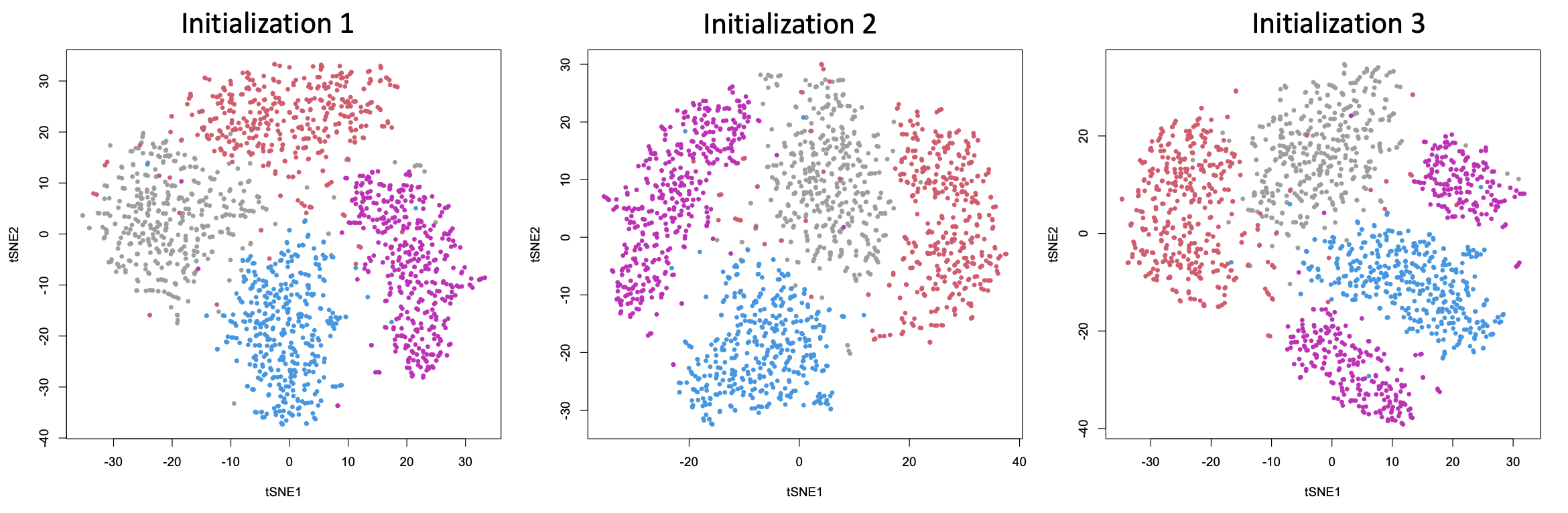
Refer to caption
Figure 6: t-SNE visualizations of 1600 MNIST samples based on three different random initializations and identical tuning parameters in (39).

Next we assess the effects and artifacts of the random initialization. In Figure 6, we fix all the tuning parameters as in (39) and generate t-SNE visualizations from three different random initializations. Comparing the first two plots, we observe that the relative positions of the clusters vary with the initialization. For example, the purple cluster and red cluster are neighbors in the left panel but not in the middle panel. This echos our theoretical prediction (discussion after Theorem 7) and justifies our second practical advice in Section 1.2. On the other hand, on the right panel of Figure 6, we find that even with a proper choice of the tuning parameters, false clustering may still appear as an artifact of the random initialization (cf. Remark 16 and the third practical advice in Section 1.2).

Finally, we point out that our theory-guided values for the tuning parameters are flexible, robust and adaptive to the sample size. For example, in Figure 10, we present three more visualizations of n=2400n=2400 (N=600N=600 for each digit) MNIST samples, by using the tuning parameters in (39) with various δ∈{1/3,1/2,2/3}\delta\in\{1/3,1/2,2/3\}, and an identical random initialization. The cluster patterns are visible and similar in all the cases, showing the effectiveness of our tuning parameters and the insensitivity to the choice of δ\delta.

6 Discussion

The present paper provides theoretical foundations of t-SNE for visualizing clustered data and obtains insights about its theoretical properties and interpretations. We believe that some of the conditions may be relaxed by adopting more advanced technical tools. For example, the current analysis of the early exaggeration stage relies on the well-celebrated Davis-Kahan matrix perturbation inequality (cf. Section B.3), which may be further improved by leveraging advanced results in Random Matrix Theory, such as Benaych-Georges and Nadakuditi 2012 and Bao et al. 2021.

There are still many interesting questions that remain to be explored. For instance, what is the limiting behavior of the low-dimensional map {yi(k)}1≤i≤n\{y_{i}^{(k)}\}_{1\leq i\leq n} towards the end of the embedding stage, after transition to the stabilization phase? How to interpret the local structure within a cluster (DePavia and Steinerberger 2020; Robinson and Pierce-Hoffman 2020)? How many iterations are needed for the embedding stage? How to determine the bandwidth {τi}\{\tau_{i}\} in a data-driven and adaptive manner (Ding and Ma 2022)? The present work is a first step towards answering these important questions.

Moreover, our theoretical framework is generic and can be generalized to study other algorithms that are closely related to or share similar features with t-SNE. For example, in addition to the variants of t-SNE mentioned in Section 1, many dimension reduction and data visualization methods, such as multidimensional scaling (Kruskal 1978), kernel principal component analysis (Schölkopf et al. 1997), and Laplacian eigenmap (Belkin and Niyogi 2003), start with a similarity matrix summarizing the pairwise distances within a dataset, and then proceed by either explicitly or implicitly exploiting the spectral properties of the similarity matrix. In this connection, the general ideas behind our theoretical analysis, such as identifying the underlying structured graph and properties of its adjacency or Laplacian matrix (Sections 2.1 and 2.2), studying the gradient flow associated with the discrete algorithm (Section 2.3), and the mechanical/kinematic view of the updating equation (Section 3), can be adopted to uncover the underlying mechanism and the properties of these methods.

It is also interesting to explore the fundamental limit for data visualization and dimension reduction. For example, what are the necessary conditions for the data {Xi}1≤i≤n\{X_{i}\}_{1\leq i\leq n} to guarantee the existence of a low-dimensional map {yi}1≤i≤n\{y_{i}\}_{1\leq i\leq n} being a metric embedding of it? Whether t-SNE has to sacrifice some global structures in order to locally embed the data well (Chari et al. 2021)? These problems are left for future investigation.

Acknowledgement

The authors are grateful to the editors and four anonymous referees for their comments and suggestions which have significantly improved the results and presentation of the paper. The research of Tony Cai was supported in part by NSF grant DMS-2015259 and NIH grant R01-GM129781. The research of Rong Ma was supported by Professor David Donoho at Stanford University. This work was partially completed while Rong Ma was a PhD candidate in Biostatistics at the University of Pennsylvania. Rong Ma would like to thank Mingyao Li for introducing the subject, and Michaël Aupetit, David Donoho, Jeyong Lee, Stefan Steinerberger, Yiqiao Zhong and James Zou for helpful discussions.

References

  • Amini and Razaee (2021) Arash A Amini and Zahra S Razaee. Concentration of kernel matrices with application to kernel spectral clustering. The Annals of Statistics, 49(1):531–556, 2021.
  • Arora et al. (2018) Sanjeev Arora, Wei Hu, and Pravesh K Kothari. An analysis of the t-SNE algorithm for data visualization. In Conference on Learning Theory, pages 1455–1462. PMLR, 2018.
  • Balakrishnan et al. (2011) Sivaraman Balakrishnan, Min Xu, Akshay Krishnamurthy, and Aarti Singh. Noise thresholds for spectral clustering. In Advances in Neural Information Processing Systems, pages 954–962, 2011.
  • Bao et al. (2021) Zhigang Bao, Xiucai Ding, and Ke Wang. Singular vector and singular subspace distribution for the matrix denoising model. The Annals of Statistics, 49(1):370–392, 2021.
  • Belkin and Niyogi (2003) Mikhail Belkin and Partha Niyogi. Laplacian eigenmaps for dimensionality reduction and data representation. Neural Computation, 15(6):1373–1396, 2003.
  • Benaych-Georges and Nadakuditi (2012) Florent Benaych-Georges and Raj Rao Nadakuditi. The singular values and vectors of low rank perturbations of large rectangular random matrices. Journal of Multivariate Analysis, 111:120–135, 2012.
  • Butcher (2008) John Charles Butcher. Numerical methods for ordinary differential equations. John Wiley & Sons, 2008.
  • Cai and Zhang (2018) T Tony Cai and Anru Zhang. Rate-optimal perturbation bounds for singular subspaces with applications to high-dimensional statistics. The Annals of Statistics, 46(1):60–89, 2018.
  • Carreira-Perpinán (2010) Miguel A Carreira-Perpinán. The elastic embedding algorithm for dimensionality reduction. In ICML, volume 10, pages 167–174, 2010.
  • Chari et al. (2021) Tara Chari, Joeyta Banerjee, and Lior Pachter. The specious art of single-cell genomics. BioRxiv, 2021.
  • Chatzimparmpas et al. (2020) Angelos Chatzimparmpas, Rafael M Martins, and Andreas Kerren. t-viSNE: Interactive assessment and interpretation of t-SNE projections. IEEE Transactions on Visualization and Computer Graphics, 26(8):2696–2714, 2020.
  • Cheng et al. (2015) Jian Cheng, Haijun Liu, Feng Wang, Hongsheng Li, and Ce Zhu. Silhouette analysis for human action recognition based on supervised temporal t-SNE and incremental learning. IEEE Transactions on Image Processing, 24(10):3203–3217, 2015.
  • DePavia and Steinerberger (2020) Adela DePavia and Stefan Steinerberger. Spectral clustering revisited: Information hidden in the fiedler vector. arXiv preprint arXiv:2003.09969, 2020.
  • Ding and Ma (2022) Xiucai Ding and Rong Ma. Learning low-dimensional nonlinear structures from high-dimensional noisy data: An integral operator approach. arXiv preprint arXiv:2203.00126, 2022.
  • Donoho (2017) David Donoho. 50 years of data science. Journal of Computational and Graphical Statistics, 26(4):745–766, 2017.
  • Gisbrecht et al. (2015) Andrej Gisbrecht, Alexander Schulz, and Barbara Hammer. Parametric nonlinear dimensionality reduction using kernel t-SNE. Neurocomputing, 147:71–82, 2015.
  • Hinton and Roweis (2002) Geoffrey Hinton and Sam T Roweis. Stochastic neighbor embedding. In Advances in Neural Information Processing Systems, volume 15, pages 833–840, 2002.
  • Im et al. (2018) Daniel Jiwoong Im, Nakul Verma, and Kristin Branson. Stochastic neighbor embedding under f-divergences. arXiv preprint arXiv:1811.01247, 2018.
  • Jacobs (1988) Robert A Jacobs. Increased rates of convergence through learning rate adaptation. Neural Networks, 1(4):295–307, 1988.
  • Kobak and Berens (2019) Dmitry Kobak and Philipp Berens. The art of using t-SNE for single-cell transcriptomics. Nature Communications, 10(1):1–14, 2019.
  • Kobak and Linderman (2021) Dmitry Kobak and George C Linderman. Initialization is critical for preserving global data structure in both t-SNE and UMAP. Nature Biotechnology, 39(2):156–157, 2021.
  • Kruskal (1978) Joseph B Kruskal. Multidimensional Scaling. Number 11. Sage, 1978.
  • Lee and Verleysen (2011) John A Lee and Michel Verleysen. Shift-invariant similarities circumvent distance concentration in stochastic neighbor embedding and variants. Procedia Computer Science, 4:538–547, 2011.
  • Lee and Verleysen (2014) John A Lee and Michel Verleysen. Two key properties of dimensionality reduction methods. In 2014 IEEE symposium on computational intelligence and data mining (CIDM), pages 163–170. IEEE, 2014.
  • Linderman and Steinerberger (2019) George C Linderman and Stefan Steinerberger. Clustering with t-SNE, provably. SIAM Journal on Mathematics of Data Science, 1(2):313–332, 2019.
  • Linderman et al. (2019) George C Linderman, Manas Rachh, Jeremy G Hoskins, Stefan Steinerberger, and Yuval Kluger. Fast interpolation-based t-SNE for improved visualization of single-cell RNA-seq data. Nature Methods, 16(3):243–245, 2019.
  • Marsden (2013) Anne Marsden. Eigenvalues of the laplacian and their relationship to the connectedness of a graph. University of Chicago, REU, 2013.
  • Nonato and Aupetit (2018) Luis Gustavo Nonato and Michael Aupetit. Multidimensional projection for visual analytics: Linking techniques with distortions, tasks, and layout enrichment. IEEE Transactions on Visualization and Computer Graphics, 25(8):2650–2673, 2018.
  • Olivon et al. (2018) Florent Olivon, Nicolas Elie, Gwendal Grelier, Fanny Roussi, Marc Litaudon, and David Touboul. Metgem software for the generation of molecular networks based on the t-SNE algorithm. Analytical Chemistry, 90(23):13900–13908, 2018.
  • Pezzotti et al. (2016) Nicola Pezzotti, Boudewijn PF Lelieveldt, Laurens Van Der Maaten, Thomas Höllt, Elmar Eisemann, and Anna Vilanova. Approximated and user steerable tSNE for progressive visual analytics. IEEE Transactions on Visualization and Computer Graphics, 23(7):1739–1752, 2016.
  • Platzer (2013) Alexander Platzer. Visualization of snps with t-SNE. PloS One, 8(2):e56883, 2013.
  • Robinson and Pierce-Hoffman (2020) Isaac Robinson and Emma Pierce-Hoffman. Tree-sne: Hierarchical clustering and visualization using t-sne. arXiv preprint arXiv:2002.05687, 2020.
  • Rudelson and Vershynin (2013) Mark Rudelson and Roman Vershynin. Hanson-wright inequality and sub-gaussian concentration. Electronic Communications in Probability, 18, 2013.
  • Schölkopf et al. (1997) Bernhard Schölkopf, Alexander Smola, and Klaus-Robert Müller. Kernel principal component analysis. In International Conference on Artificial Neural Networks, pages 583–588. Springer, 1997.
  • Shaham and Steinerberger (2017) Uri Shaham and Stefan Steinerberger. Stochastic neighbor embedding separates well-separated clusters. arXiv preprint arXiv:1702.02670, 2017.
  • Traven et al. (2017) Gregor Traven, Gal Matijevič, Tomaz Zwitter, M Žerjal, Janez Kos, Martin Asplund, Joss Bland-Hawthorn, Andrew R Casey, Gayandhi De Silva, Kenneth Freeman, et al. The galah survey: classification and diagnostics with t-SNE reduction of spectral information. The Astrophysical Journal Supplement Series, 228(2):24, 2017.
  • van der Maaten (2014) Laurens van der Maaten. Accelerating t-SNE using tree-based algorithms. The Journal of Machine Learning Research, 15(1):3221–3245, 2014.
  • van der Maaten and Hinton (2008) Laurens van der Maaten and Geoffrey Hinton. Visualizing data using t-SNE. Journal of Machine Learning Research, 9(Nov):2579–2605, 2008.
  • Varga (2010) Richard S Varga. Geršgorin and his circles, volume 36. Springer Science & Business Media, 2010.
  • Wang et al. (2021) Yingfan Wang, Haiyang Huang, Cynthia Rudin, and Yaron Shaposhnik. Understanding how dimension reduction tools work: An empirical approach to deciphering t-sne, umap, trimap, and pacmap for data visualization. Journal of Machine Learning Research, 22:1–73, 2021.
  • Xie et al. (2011) Bo Xie, Yang Mu, Dacheng Tao, and Kaiqi Huang. m-SNE: Multiview stochastic neighbor embedding. IEEE Transactions on Systems, Man, and Cybernetics, Part B (Cybernetics), 41(4):1088–1096, 2011.
  • Yang et al. (2009) Zhirong Yang, Irwin King, Zenglin Xu, and Erkki Oja. Heavy-tailed symmetric stochastic neighbor embedding. In Advances in Neural Information Processing Systems, volume 22, pages 2169–2177, 2009.
  • Zhang and Steinerberger (2021) Yulan Zhang and Stefan Steinerberger. t-SNE, forceful colorings and mean field limits. arXiv preprint arXiv:2102.13009, 2021.

Appendix A Discrete-Time Analysis of the Early Exaggeration Stage

A.1 Proof of Theorem 2

For simplicity, we ignore the superscript (k)(k) in yi(k),qi​j(k),η(k)y_{i}^{(k)},q_{ij}^{(k)},\eta^{(k)} and Si​j(k)​(α)S_{ij}^{(k)}(\alpha). Since Si​j​(α)=α​pi​j−qi​j1+‖yi−yj‖22,S_{ij}(\alpha)=\frac{\alpha p_{ij}-q_{ij}}{1+\|y_{i}-y_{j}\|_{2}^{2}}, if we denote di​j=‖yi−yj‖22d_{ij}=\|y_{i}-y_{j}\|_{2}^{2}, we have

|Si​j​(α)−α​pi​j+1n⁡(n−1)|\displaystyle\bigg|S_{ij}(\alpha)-{\alpha p_{ij}}+\frac{1}{n(n-1)}\bigg| ≤|α​pi​j−α​pi​j1+di​j|+|qi​j1+di​j−1n⁡(n−1)|\displaystyle\leq|{\alpha p_{ij}}-\frac{\alpha p_{ij}}{1+d_{ij}}|+\bigg|\frac{q_{ij}}{1+d_{ij}}-\frac{1}{n(n-1)}\bigg|
=di​j​α​pi​j+|1Z​(1+di​j)2−1n⁡(n−1)|,\displaystyle=d_{ij}\alpha p_{ij}+\bigg|\frac{1}{Z(1+d_{ij})^{2}}-\frac{1}{n(n-1)}\bigg|,

where

Z=∑i≠j(1+di​j)−1=∑i≠j(1−di​j1+di​j)=n⁡(n−1)−∑i≠jdi​j1+di​j≡n⁡(n−1)−Δ.Z=\sum_{i\neq j}(1+d_{ij})^{-1}=\sum_{i\neq j}\bigg(1-\frac{d_{ij}}{1+d_{ij}}\bigg)=n(n-1)-\sum_{i\neq j}\frac{d_{ij}}{1+d_{ij}}\equiv n(n-1)-\Delta.

Now since Δ≤n⁡(n−1)​min⁡{η,1}=n⁡(n−1)​η\Delta\leq n(n-1)\min\{\eta,1\}=n(n-1)\eta, we have

|1Z​(1+di​j)2−1n⁡(n−1)|=|(1+di​j)−2​n​(n−1)−n⁡(n−1)+Δn2​(n−1)2−n⁡(n−1)​Δ|\displaystyle\bigg|\frac{1}{Z(1+d_{ij})^{2}}-\frac{1}{n(n-1)}\bigg|=\bigg|\frac{(1+d_{ij})^{-2}n(n-1)-n(n-1)+\Delta}{n^{2}(n-1)^{2}-n(n-1)\Delta}\bigg|
≤|[(1+di​j)−2−1]​n​(n−1)+Δ|n2​(n−1)2​(1−η)≤2​ηn​(n−1)​(1−η)\displaystyle\leq\frac{|[(1+d_{ij})^{-2}-1]n(n-1)+\Delta|}{n^{2}(n-1)^{2}(1-\eta)}\leq\frac{2\eta}{n(n-1)(1-\eta)} (40)

Hence

|Si​j​(α)−α​pi​j+1n⁡(n−1)|≤η​α​pi​j+2​ηn​(n−1)​(1−η).\bigg|S_{ij}(\alpha)-{\alpha p_{ij}}+\frac{1}{n(n-1)}\bigg|\leq\eta\alpha p_{ij}+\frac{2\eta}{n(n-1)(1-\eta)}.

For the second statement, we note that

‖ℍn‖≤1n−1+1n⁡(n−1)≲1n.\|\mathbb{H}_{n}\|\leq\frac{1}{n-1}+\frac{1}{n(n-1)}\lesssim\frac{1}{n}. (41)

Then as long as ‖α​ℙ‖≫1n\|\alpha\mathbb{P}\|\gg\frac{1}{n}, we have ‖α​ℙ−ℍn‖≥‖α​ℙ‖−1n≍‖α​ℙ‖.\|\alpha\mathbb{P}-\mathbb{H}_{n}\|\geq\|\alpha\mathbb{P}\|-\frac{1}{n}\asymp\|\alpha\mathbb{P}\|. Therefore, under the condition that η≪‖ℙ‖n​‖ℙ‖∞≤1\eta\ll{\frac{\|\mathbb{P}\|}{n\|\mathbb{P}\|_{\infty}}}\leq 1,

‖𝕊α−(α​ℙ−ℍn)‖‖α​ℙ−ℍn‖\displaystyle\frac{\|\mathbb{S}_{\alpha}-(\alpha\mathbb{P}-\mathbb{H}_{n})\|}{\|\alpha\mathbb{P}-\mathbb{H}_{n}\|} ≲n​‖𝕊α−(α​ℙ−ℍn)‖∞‖α​ℙ‖≲α​n​‖ℙ‖∞​η+η/n‖α​ℙ‖\displaystyle\lesssim\frac{n\|\mathbb{S}_{\alpha}-(\alpha\mathbb{P}-\mathbb{H}_{n})\|_{\infty}}{\|\alpha\mathbb{P}\|}\lesssim\frac{\alpha n\|\mathbb{P}\|_{\infty}\eta+\eta/n}{\|\alpha\mathbb{P}\|}

Then, the first term η​n​‖ℙ‖∞/‖ℙ‖→0{\eta n\|\mathbb{P}\|_{\infty}}/{\|\mathbb{P}\|}\to 0 as η≪‖ℙ‖/(n​‖ℙ‖∞)\eta\ll\|\mathbb{P}\|/(n\|\mathbb{P}\|_{\infty}); the second term ηn​α​‖ℙ‖≲1n​α​‖ℙ‖→0\frac{\eta}{n\alpha\|\mathbb{P}\|}\lesssim\frac{1}{n\alpha\|\mathbb{P}\|}\to 0 as α≫(n​‖ℙ‖)−1\alpha\gg(n\|\mathbb{P}\|)^{-1}.

A.2 Proof of Proposition 3

Note that yℓ​i(k+1)≤‖[𝐈−h​𝕃​(𝕊α(k))]i.‖1​‖𝒚ℓ(k)‖∞y_{\ell i}^{(k+1)}\leq\|[{\bf I}-h\mathbb{L}(\mathbb{S}^{(k)}_{\alpha})]_{i.}\|_{1}\|\boldsymbol{y}_{\ell}^{(k)}\|_{\infty} for any k≥0k\geq 0, where

‖[𝐈−h​𝕃​(𝕊α(k))]i.‖1\displaystyle\|[{\bf I}-h\mathbb{L}(\mathbb{S}^{(k)}_{\alpha})]_{i.}\|_{1} =|1−h​∑j=1nSi​j(k)​(α)|+h​∑j≠i|Si​j(k)​(α)|≤1+2​h​∑j=1n|Si​j(k)​(α)|.\displaystyle=\bigg|1-h\sum_{j=1}^{n}S_{ij}^{(k)}(\alpha)\bigg|+h\sum_{j\neq i}|S_{ij}^{(k)}(\alpha)|\leq 1+2h\sum_{j=1}^{n}|S_{ij}^{(k)}(\alpha)|.

For the last term, we have

h​∑j=1n|Si​j(k)​(α)|≤h​n​‖𝕊α(k)‖∞≤n​h​(α​‖ℙ‖∞+‖ℚ(k)‖∞)≤n​h​α​‖ℙ‖∞+h⁡(1+η(k))n−1h\sum_{j=1}^{n}|S_{ij}^{(k)}(\alpha)|\leq hn\|\mathbb{S}_{\alpha}^{(k)}\|_{\infty}\leq nh(\alpha\|\mathbb{P}\|_{\infty}+\|\mathbb{Q}^{(k)}\|_{\infty})\leq nh\alpha\|\mathbb{P}\|_{\infty}+\frac{h(1+\eta^{(k)})}{n-1}

where the last inequality follows from (40), that is, ‖ℚ(k)‖∞≤1/Z\|\mathbb{Q}^{(k)}\|_{\infty}\leq 1/Z, Z≥n⁡(n−1)/(1+η(k))Z\geq n(n-1)/(1+\eta^{(k)}), so that ‖ℚ(k)‖∞≤(1+η(k))/n⁡(n−1)\|\mathbb{Q}^{(k)}\|_{\infty}\leq(1+\eta^{(k)})/n(n-1). Then we have

yℓ​i(k+1)≤(1+2​n​h​α​‖ℙ‖∞+2​h​(1+η(k))n−1)​‖𝒚ℓ(k)‖∞,y_{\ell i}^{(k+1)}\leq\bigg(1+2nh\alpha\|\mathbb{P}\|_{\infty}+\frac{2h(1+\eta^{(k)})}{n-1}\bigg)\|\boldsymbol{y}_{\ell}^{(k)}\|_{\infty},

or

‖𝒚ℓ(k+1)‖∞≤(1+2​n​h​α​‖ℙ‖∞+2​h​(1+η(k))n−1)​‖𝒚ℓ(k)‖∞.\|\boldsymbol{y}_{\ell}^{(k+1)}\|_{\infty}\leq\bigg(1+2nh\alpha\|\mathbb{P}\|_{\infty}+\frac{2h(1+\eta^{(k)})}{n-1}\bigg)\|\boldsymbol{y}_{\ell}^{(k)}\|_{\infty}.

Whenever η(k)\eta^{(k)} and max⁡{‖𝒚1(k)‖∞,‖𝒚2(k)‖∞}\max\{\|\boldsymbol{y}_{1}^{(k)}\|_{\infty},\|\boldsymbol{y}_{2}^{(k)}\|_{\infty}\} are bounded by an absolute constant, by setting rn=n​h​α​‖ℙ‖∞+hnr_{n}=nh\alpha\|\mathbb{P}\|_{\infty}+\frac{h}{n} and assuming rn=O⁡(1)r_{n}=O(1) (by Condition (T1)), we have

‖𝒚ℓ(k+1)‖∞≤(1+C​rn)​‖𝒚ℓ(k)‖∞,\|\boldsymbol{y}_{\ell}^{(k+1)}\|_{\infty}\leq(1+Cr_{n})\|\boldsymbol{y}_{\ell}^{(k)}\|_{\infty}, (42)

and

η(k+1)≤4​maxi∈[n],ℓ∈[2]​|yi​ℓ(k)|2≤8​max⁡{‖𝒚1(k+1)‖∞2,‖𝒚2(k+1)‖∞2}\displaystyle\eta^{(k+1)}\leq 4\max_{i\in[n],\ell\in[2]}|y_{i\ell}^{(k)}|^{2}\leq 8\max\{\|\boldsymbol{y}_{1}^{(k+1)}\|^{2}_{\infty},\|\boldsymbol{y}_{2}^{(k+1)}\|^{2}_{\infty}\}
≤8​(1+C​rn)​max⁡{‖𝒚1(k)‖∞2,‖𝒚2(k)‖∞2}=O⁡(1)\displaystyle\leq 8(1+Cr_{n})\max\{\|\boldsymbol{y}_{1}^{(k)}\|^{2}_{\infty},\|\boldsymbol{y}_{2}^{(k)}\|^{2}_{\infty}\}=O(1)

In other words, we have shown that for any kk such that η(k)\eta^{(k)} and max⁡{‖𝒚1(k)‖∞,‖𝒚2(k)‖∞}\max\{\|\boldsymbol{y}_{1}^{(k)}\|_{\infty},\|\boldsymbol{y}_{2}^{(k)}\|_{\infty}\} are bounded, then (42) holds, and η(k+1)\eta^{(k+1)} and max⁡{‖𝒚1(k+1)‖∞,‖𝒚2(k+1)‖∞}\max\{\|\boldsymbol{y}_{1}^{(k+1)}\|_{\infty},\|\boldsymbol{y}_{2}^{(k+1)}\|_{\infty}\} are bounded.

Now Condition (I1) says that max⁡{‖𝒚1(0)‖∞,‖𝒚2(0)‖∞}=O⁡(1)\max\{\|\boldsymbol{y}_{1}^{(0)}\|_{\infty},\|\boldsymbol{y}_{2}^{(0)}\|_{\infty}\}=O(1) and η(0)≤4​maxℓ∈[2]​‖𝒚ℓ(0)‖∞2=O⁡(1)\eta^{(0)}\leq 4\max_{\ell\in[2]}\|\boldsymbol{y}_{\ell}^{(0)}\|_{\infty}^{2}=O(1). By induction, we know that η(k)\eta^{(k)} and max⁡{‖𝒚1(k+1)‖∞,‖𝒚2(k+1)‖∞}\max\{\|\boldsymbol{y}_{1}^{(k+1)}\|_{\infty},\|\boldsymbol{y}_{2}^{(k+1)}\|_{\infty}\} are bounded and (42) holds for all k≥1k\geq 1. Applying (42) iteratively, we have for any k≥1k\geq 1,

‖𝒚ℓ(k)‖∞≤(1+C​rn)k​‖𝒚ℓ(0)‖∞.\|\boldsymbol{y}_{\ell}^{(k)}\|_{\infty}\leq(1+Cr_{n})^{k}\|\boldsymbol{y}_{\ell}^{(0)}\|_{\infty}. (43)

Therefore, as long as k=k⁡(n)k=k(n) such that k​rn=O⁡(1)kr_{n}=O(1) (by Condition (T1)), we have ‖𝒚ℓ(k)‖∞/‖𝒚ℓ(0)‖∞=O⁡(1),{\|\boldsymbol{y}_{\ell}^{(k)}\|_{\infty}}/{\|\boldsymbol{y}_{\ell}^{(0)}\|_{\infty}}=O(1), or

diam​({yi(k)}1≤i≤n)maxi∈[n],ℓ∈[2]⁡|yi​ℓ(0)|≤maxi∈[n],ℓ∈[2]⁡|yi​ℓ(k)|maxi∈[n],ℓ∈[2]⁡|yi​ℓ(0)|=O⁡(1).\frac{\text{diam}(\{y_{i}^{(k)}\}_{1\leq i\leq n})}{\max_{i\in[n],\ell\in[2]}|y_{i\ell}^{(0)}|}\leq\frac{\max_{i\in[n],\ell\in[2]}|y_{i\ell}^{(k)}|}{\max_{i\in[n],\ell\in[2]}|y_{i\ell}^{(0)}|}=O(1).

A.3 Proof of Theorem 4

The results concerning (10) and (12) follows directly from Theorem 2 and Proposition 3. To see that (13) holds, we first prove the following proposition.

Proposition 20.

Let 𝔼α(k)=𝕊α(k)−(α​ℙ−ℍn)\mathbb{E}_{\alpha}^{(k)}=\mathbb{S}_{\alpha}^{(k)}-(\alpha\mathbb{P}-\mathbb{H}_{n}) and ζ=supk≥0‖𝕃⁡(𝔼α(k))‖\zeta=\sup_{k\geq 0}\|\mathbb{L}(\mathbb{E}_{\alpha}^{(k)})\|. Suppose the initialization satisfies ‖𝐲ℓ(0)‖≠0\|\boldsymbol{y}_{\ell}^{(0)}\|\neq 0 for ℓ=1,2\ell=1,2, and (α,h,K)(\alpha,h,K) satisfies h​‖𝕃⁡(α​ℙ)‖<2h\|\mathbb{L}(\alpha\mathbb{P})\|<2, K​h​ζ=O⁡(1)Kh\zeta=O(1) and K​h=O⁡(n)Kh=O(n) as n→∞n\to\infty. Then for ℓ∈{1,2}\ell\in\{1,2\}, it holds that

sup1≤k≤K‖𝒚ℓ(k)−[𝐈−h​𝕃​(α​ℙ−ℍn)]k​𝒚ℓ(0)‖2‖𝒚ℓ(0)‖2=O⁡(K​h​ζ).\sup_{1\leq k\leq K}\frac{\|\boldsymbol{y}_{\ell}^{(k)}-[{\bf I}-h\mathbb{L}(\alpha\mathbb{P}-\mathbb{H}_{n})]^{k}\boldsymbol{y}_{\ell}^{(0)}\|_{2}}{\|\boldsymbol{y}_{\ell}^{(0)}\|_{2}}=O(Kh\zeta). (44)

Consequently, for (α,h,k)(\alpha,h,k) such that h​‖𝕃⁡(α​ℙ)‖<2h\|\mathbb{L}(\alpha\mathbb{P})\|<2, k​h​ζ=o⁡(1)kh\zeta=o(1) and k​h=O⁡(n)kh=O(n), we have

limn→∞‖𝒚ℓ(k)−[𝐈−h​𝕃​(α​ℙ−ℍn)]k​𝒚ℓ(0)‖2‖𝒚ℓ(0)‖2=0.\lim_{n\to\infty}\frac{\|\boldsymbol{y}_{\ell}^{(k)}-[{\bf I}-h\mathbb{L}(\alpha\mathbb{P}-\mathbb{H}_{n})]^{k}\boldsymbol{y}_{\ell}^{(0)}\|_{2}}{\|\boldsymbol{y}_{\ell}^{(0)}\|_{2}}=0. (45)
Proof.

By linearity of the Laplacian operator, we have

𝕃⁡(𝔼α(k))=𝕃⁡(𝕊α(k))−𝕃⁡(α​ℙ−ℍn)=𝕃⁡(𝕊α(k))−𝕃⁡(α​ℙ−ℍn)\mathbb{L}(\mathbb{E}_{\alpha}^{(k)})=\mathbb{L}(\mathbb{S}_{\alpha}^{(k)})-\mathbb{L}(\alpha\mathbb{P}-\mathbb{H}_{n})=\mathbb{L}(\mathbb{S}_{\alpha}^{(k)})-\mathbb{L}(\alpha\mathbb{P}-\mathbb{H}_{n})

For ℓ=1,2,\ell=1,2, the updating equation 𝒚ℓ(k+1)=(𝐈−h​𝕃​(𝕊α(k)))​𝒚ℓ(k)\boldsymbol{y}_{\ell}^{(k+1)}=({\bf I}-h\mathbb{L}(\mathbb{S}_{\alpha}^{(k)}))\boldsymbol{y}_{\ell}^{(k)} can be written as

𝒚ℓ(k+1)\displaystyle\boldsymbol{y}_{\ell}^{(k+1)} =(𝐈−h​𝕃​(𝕊α(k)))​(𝐈−h​𝕃​(𝕊α(k−1)))​…​(𝐈−h​𝕃​(𝕊α(0)))​𝒚ℓ(0)\displaystyle=({\bf I}-h\mathbb{L}(\mathbb{S}_{\alpha}^{(k)}))({\bf I}-h\mathbb{L}(\mathbb{S}_{\alpha}^{(k-1)}))...({\bf I}-h\mathbb{L}(\mathbb{S}_{\alpha}^{(0)}))\boldsymbol{y}_{\ell}^{(0)}
=(𝐈−h​𝕃​(α​ℙ−ℍn)−h​𝕃​(𝔼α(k)))​(𝐈−h​𝕃​(α​ℙ−ℍn)−𝕃⁡(𝔼α(k−1)))​…\displaystyle=({\bf I}-h\mathbb{L}(\alpha\mathbb{P}-\mathbb{H}_{n})-h\mathbb{L}(\mathbb{E}_{\alpha}^{(k)}))({\bf I}-h\mathbb{L}(\alpha\mathbb{P}-\mathbb{H}_{n})-\mathbb{L}(\mathbb{E}_{\alpha}^{(k-1)}))...
×(𝐈−h​𝕃​(α​ℙ−ℍn)−𝕃⁡(𝔼α(0)))​𝒚ℓ(0)\displaystyle\quad\times({\bf I}-h\mathbb{L}(\alpha\mathbb{P}-\mathbb{H}_{n})-\mathbb{L}(\mathbb{E}_{\alpha}^{(0)}))\boldsymbol{y}_{\ell}^{(0)}
=(𝐈−h​𝕃​(α​ℙ−ℍn))k+1​𝒚ℓ(0)+ϵ(k),\displaystyle=({\bf I}-h\mathbb{L}(\alpha\mathbb{P}-\mathbb{H}_{n}))^{k+1}\boldsymbol{y}_{\ell}^{(0)}+\boldsymbol{\epsilon}^{(k)},

where

‖ϵ(k)‖2\displaystyle\|\boldsymbol{\epsilon}^{(k)}\|_{2} ≤‖𝒚ℓ(0)‖2​[(k+11)​h​ζ​λk+(k+12)​(h​ζ)2​λk−1+…+(k+1k+1)​(h​ζ)k+1​λ0]\displaystyle\leq\|\boldsymbol{y}_{\ell}^{(0)}\|_{2}\bigg[{k+1\choose 1}h\zeta\lambda^{k}+{k+1\choose 2}(h\zeta)^{2}\lambda^{k-1}+...+{k+1\choose k+1}(h\zeta)^{k+1}\lambda^{0}\bigg]
≤‖𝒚ℓ(0)‖2​[(h​ζ+λ)k+1−λk+1]\displaystyle\leq\|\boldsymbol{y}_{\ell}^{(0)}\|_{2}[(h\zeta+\lambda)^{k+1}-\lambda^{k+1}]
≤‖𝒚ℓ(0)‖2​λk+1​[(h​ζ/λ+1)k+1−1]\displaystyle\leq\|\boldsymbol{y}_{\ell}^{(0)}\|_{2}\lambda^{k+1}[({h\zeta}/{\lambda}+1)^{k+1}-1]

where λ=‖𝐈−h​𝕃​(α​ℙ−ℍn)‖\lambda=\|{\bf I}-h\mathbb{L}(\alpha\mathbb{P}-\mathbb{H}_{n})\| and ζ=supk≥0‖𝕃⁡(𝔼α(k))‖\zeta=\sup_{k\geq 0}\|\mathbb{L}(\mathbb{E}_{\alpha}^{(k)})\|. We need the following lemma.

Lemma 21.

If ‖h​𝕃​(α​ℙ)‖<2\|h\mathbb{L}(\alpha\mathbb{P})\|<2, then 1≤‖𝐈−h​𝕃​(α​ℙ−ℍn)‖≤1+hn−11\leq\|{\bf I}-h\mathbb{L}(\alpha\mathbb{P}-\mathbb{H}_{n})\|\leq 1+\frac{h}{n-1}.

The above lemma implies

∥ϵ(k)∥2≤∥𝒚ℓ(0)∥2(1+Ch/n))k+1[(hζ+1)k+1−1.\|\boldsymbol{\epsilon}^{(k)}\|_{2}\leq\|\boldsymbol{y}_{\ell}^{(0)}\|_{2}(1+Ch/n))^{k+1}[({h\zeta}+1)^{k+1}-1.

By the binomial identity,

(1+xn)k\displaystyle(1+x_{n})^{k} =1+k​xn+k⁡(k−1)2​xn2+k​(k−1)​(k−2)3!​xn3+…+xnk\displaystyle=1+kx_{n}+\frac{k(k-1)}{2}x_{n}^{2}+\frac{k(k-1)(k-2)}{3!}x_{n}^{3}+...+x_{n}^{k}
≤1+k​xn+k22​xn2+k33!​xn3+…+kkk!​xnk\displaystyle\leq 1+kx_{n}+\frac{k^{2}}{2}x_{n}^{2}+\frac{k^{3}}{3!}x_{n}^{3}+...+\frac{k^{k}}{k!}x_{n}^{k}
≤1+k​xn​(1+k​xn+k2​xn22!+…+kk−1​xnk−1(k−1)!)\displaystyle\leq 1+kx_{n}\bigg(1+kx_{n}+\frac{k^{2}x_{n}^{2}}{2!}+...+\frac{k^{k-1}x_{n}^{k-1}}{(k-1)!}\bigg)
≤1+k​xn​ek​xn.\displaystyle\leq 1+kx_{n}e^{kx_{n}}.

Then, as long as k​h​ζ=O⁡(1)kh\zeta=O(1) as n→∞n\to\infty, there exits some universal constant C>0C>0 such that, for all nn,

(1+h​ζ)k+1−1≤C​k​h​ζ.(1+h\zeta)^{k+1}-1\leq Ckh\zeta. (46)

Similarly, whenever k​h/n=O⁡(1)kh/n=O(1), we have OPEN(1+C​h/n))k+1≤C(1+Ch/n))^{k+1}\leq C. Hence, we have ‖ϵ(k)‖2/‖𝒚ℓ(0)‖2≤C​k​h​ζ.{\|\boldsymbol{\epsilon}^{(k)}\|_{2}}/{\|\boldsymbol{y}_{\ell}^{(0)}\|_{2}}\leq Ckh\zeta. This proves the theorem. ∎

By the above proposition, it suffices to reduce the following full list of conditions – α≫1n​‖ℙ‖\alpha\gg\frac{1}{n\|\mathbb{P}\|}, k​h=O⁡(n)kh=O(n), n​h​α​‖ℙ‖∞<1nh\alpha\|\mathbb{P}\|_{\infty}<1, maxi∈[n],ℓ∈[2]⁡|yi​ℓ(0)|2=o⁡(‖ℙ‖/(n​‖ℙ‖∞))\max_{i\in[n],\ell\in[2]}|y_{i\ell}^{(0)}|^{2}=o(\|\mathbb{P}\|/(n\|\mathbb{P}\|_{\infty})), ‖𝒚ℓ(0)‖≠0\|\boldsymbol{y}_{\ell}^{(0)}\|\neq 0 for ℓ∈{1,2}\ell\in\{1,2\}, k⁡(n​h​α​‖ℙ‖∞+h/n)=O⁡(1)k(nh\alpha\|\mathbb{P}\|_{\infty}+h/n)=O(1), and k⁡(n​h​α​‖ℙ‖∞+h/n)⋅maxi∈[n],ℓ∈[2]⁡|yi​ℓ(0)|2=O⁡(1)k(nh\alpha\|\mathbb{P}\|_{\infty}+h/n)\cdot\max_{i\in[n],\ell\in[2]}|y_{i\ell}^{(0)}|^{2}=O(1) – to those in (I1) (I2) and (T1.D). To see this, note that k⁡(n​h​α​‖ℙ‖∞+h/n)⋅maxi∈[n],ℓ∈[2]⁡|yi​ℓ(0)|2→0k\big(nh\alpha\|\mathbb{P}\|_{\infty}+{h}/{n}\big)\cdot\max_{i\in[n],\ell\in[2]}|y_{i\ell}^{(0)}|^{2}\to 0, can be implied by

k⁡(n​h​α​‖ℙ‖∞+h/n)=o⁡(1),maxi∈[n],ℓ∈[2]⁡|yi​ℓ(0)|2≪‖ℙ‖/(n​‖ℙ‖∞)≤1.k\big(nh\alpha\|\mathbb{P}\|_{\infty}+{h}/{n}\big)=o(1),\quad\max_{i\in[n],\ell\in[2]}|y_{i\ell}^{(0)}|^{2}\ll\|\mathbb{P}\|/(n\|\mathbb{P}\|_{\infty})\leq 1.

In addition, k​h=O⁡(n)kh=O(n) and α​h​n​‖ℙ‖∞<1\alpha hn\|\mathbb{P}\|_{\infty}<1 can be implied by the above first inequality.

A.4 Proof of Theorem 5

Since 𝕃⁡(ℍn)=1n−1​𝐈n−1n⁡(n−1)​𝟏n​𝟏n⊤,\mathbb{L}(\mathbb{H}_{n})=\frac{1}{n-1}{\bf I}_{n}-\frac{1}{n(n-1)}{\bf 1}_{n}{\bf 1}_{n}^{\top}, it follows that

𝐈n−h​𝕃​(ℙ−ℍn)=𝐈n−h​𝕃​(ℙ)+hn−1​𝐈n−hn⁡(n−1)​𝟏n​𝟏n⊤.{\bf I}_{n}-h\mathbb{L}(\mathbb{P}-\mathbb{H}_{n})={\bf I}_{n}-h\mathbb{L}(\mathbb{P})+\frac{h}{n-1}{\bf I}_{n}-\frac{h}{n(n-1)}{\bf 1}_{n}{\bf 1}_{n}^{\top}. (47)

Without loss of generality, we assume R≥2R\geq 2, as the case for R=1R=1 follows similarly. Let 𝕦i\mathbb{u}_{i} be the ii-th column of 𝕌′∈O⁡(n,R−1)\mathbb{U}^{\prime}\in O(n,R-1), which consists of the eigenvectors corresponding to the eigenvalue 00 of 𝕃⁡(ℙ)\mathbb{L}(\mathbb{P}) other than the trivial eigenvector n−1/2𝟏nn^{-1/2}{\bf 1}_{n}, and let 𝕌\mathbb{U} be the matrix that binds an additional column n−1/2𝟏nn^{-1/2}{\bf 1}_{n} to 𝕌′\mathbb{U}^{\prime}. Let λ1≤…≤λn\lambda_{1}\leq...\leq\lambda_{n} be the eigenvalues of 𝕃⁡(ℙ)\mathbb{L}(\mathbb{P}), with λ1=…=λR=0\lambda_{1}=...=\lambda_{R}=0. Then it follows that

𝐈−h​𝕃​(ℙ−ℍn)\displaystyle{\bf I}-h\mathbb{L}(\mathbb{P}-\mathbb{H}_{n})
=[𝕌′n−1/2𝟏n𝕌⟂][1+hn−1−h​λ1⋱1+hn−1−h​λR−11+hn−1−h​λR1+hn−1−h​λR+1⋱1+hn−1−h​λn]\displaystyle=[\mathbb{U}^{\prime}\quad n^{-1/2}{\bf 1}_{n}\quad\mathbb{U}_{\perp}]{\tiny\begin{bmatrix}1+\frac{h}{n-1}-h\lambda_{1}&&&&&&\\ &\ddots&&&&&\\ &&1+\frac{h}{n-1}-h\lambda_{R-1}&&&&\\ &&&1+\frac{h}{n-1}-h\lambda_{R}&&&\\ &&&&1+\frac{h}{n-1}-h\lambda_{R+1}&&\\ &&&&&\ddots&\\ &&&&&&1+\frac{h}{n-1}-h\lambda_{n}\end{bmatrix}}
×[𝕌′n−1/2𝟏𝕌⟂]⊤−hn⁡(n−1)𝟏𝟏⊤\displaystyle\quad\times[\mathbb{U}^{\prime}\quad n^{-1/2}{\bf 1}\quad\mathbb{U}_{\perp}]^{\top}-\frac{h}{n(n-1)}{\bf 11}^{\top}
=[𝕌′n−1/2𝟏𝕌⟂][1+hn−1⋱1+hn−111+hn−1−h​λR+1⋱1+hn−1−h​λn][𝕌′n−1/2𝟏𝕌⟂]⊤\displaystyle=[\mathbb{U}^{\prime}\quad n^{-1/2}{\bf 1}\quad\mathbb{U}_{\perp}]{\tiny\begin{bmatrix}1+\frac{h}{n-1}&&&&&&\\ &\ddots&&&&&\\ &&1+\frac{h}{n-1}&&&&\\ &&&1&&&\\ &&&&1+\frac{h}{n-1}-h\lambda_{R+1}&&\\ &&&&&\ddots&\\ &&&&&&1+\frac{h}{n-1}-h\lambda_{n}\end{bmatrix}}[\mathbb{U}^{\prime}\quad n^{-1/2}{\bf 1}\quad\mathbb{U}_{\perp}]^{\top}

Then if we denote 𝕦R+1,…,𝕦n\mathbb{u}_{R+1},...,\mathbb{u}_{n} as the columns of 𝕌⟂\mathbb{U}_{\perp}, we have

(𝐈−h​𝕃​(ℙ−ℍn))k=∑i=1R−1(1+hn−1)k​𝕦i​𝕦i⊤+n−1​𝟏𝟏⊤+∑i=R+1n(1+hn−1−h​λi)k​𝕦i​𝕦i⊤.({\bf I}-h\mathbb{L}(\mathbb{P}-\mathbb{H}_{n}))^{k}=\sum_{i=1}^{R-1}\bigg(1+\frac{h}{n-1}\bigg)^{k}\mathbb{u}_{i}\mathbb{u}_{i}^{\top}+n^{-1}{\bf 11}^{\top}+\sum_{i=R+1}^{n}\bigg(1+\frac{h}{n-1}-h\lambda_{i}\bigg)^{k}\mathbb{u}_{i}\mathbb{u}_{i}^{\top}.

Hence

‖(𝐈−h​𝕃)k​𝒚−(1+hn−1)k​∑i=1R−1𝕦i​𝕦i⊤​𝒚−n−1​𝟏𝟏⊤​𝒚‖2=‖∑i=R+1n(1+hn−1−h​λi)k​𝕦i​𝕦i⊤​𝒚‖2\displaystyle\bigg\|({\bf I}-h\mathbb{L})^{k}\boldsymbol{y}-\bigg(1+\frac{h}{n-1}\bigg)^{k}\sum_{i=1}^{R-1}\mathbb{u}_{i}\mathbb{u}_{i}^{\top}\boldsymbol{y}-n^{-1}{\bf 11}^{\top}\boldsymbol{y}\bigg\|_{2}=\bigg\|\sum_{i=R+1}^{n}\bigg(1+\frac{h}{n-1}-h\lambda_{i}\bigg)^{k}\mathbb{u}_{i}\mathbb{u}_{i}^{\top}\boldsymbol{y}\bigg\|_{2}
=∑i=R+1n(1+hn−1−h​λi)2​k​(𝕦i⊤​𝒚)2≤(1+hn−1−h​λR+1)k​‖𝒚‖2.\displaystyle=\sqrt{\sum_{i=R+1}^{n}\bigg(1+\frac{h}{n-1}-h\lambda_{i}\bigg)^{2k}(\mathbb{u}_{i}^{\top}\boldsymbol{y})^{2}}\leq\bigg(1+\frac{h}{n-1}-h\lambda_{R+1}\bigg)^{k}\|\boldsymbol{y}\|_{2}.

The final result follows by noting that 1+hn−1−h​λR+1<1−κ/2<1.1+\frac{h}{n-1}-h\lambda_{R+1}<1-\kappa/2<1.

A.5 Proof of Proposition 6

Firstly, since 𝔸\mathbb{A} is nonnegative, by the Geršgorin circle theorem (Varga 2010), 𝕃⁡(𝔸)\mathbb{L}(\mathbb{A}) is positive semi-definite. For any 𝜽r\boldsymbol{\theta}_{r}, r∈{1,…,R}r\in\{1,...,R\}, it holds that 𝕃⁡(ℙ)​𝜽r=0.\mathbb{L}(\mathbb{P})\boldsymbol{\theta}_{r}=0. It follows that {𝜽r}r=1R\{\boldsymbol{\theta}_{r}\}_{r=1}^{R} is a set of eigenvectors corresponding to the smallest eigenvalue 00. In addition, since the graph corresponding to the weighted adjacency matrix ℙ\mathbb{P} has RR connected components, by the spectral property of the Laplacian matrix (see, for example, Theorem 3.10 of Marsden 2013), the null space of 𝕃⁡(ℙ)\mathbb{L}(\mathbb{P}) has dimension RR. This implies that the eigenvalue 00 of 𝕃⁡(ℙ)\mathbb{L}(\mathbb{P}) has multiplicity RR. Lastly, as {𝜽k}k=1K\{\boldsymbol{\theta}_{k}\}_{k=1}^{K} are linearly independent, the eigen subspace associated with the eigenvalue 00 is spanned by {𝜽r}r=1R\{\boldsymbol{\theta}_{r}\}_{r=1}^{R}.

A.6 Proof of Theorem 7

Let 𝔼′α(k)=𝕊α(k)−α​ℙ∗+ℍn{\mathbb{E}^{\prime}}_{\alpha}^{(k)}=\mathbb{S}_{\alpha}^{(k)}-\alpha\mathbb{P}^{*}+\mathbb{H}_{n} and ζ′=supk≥1‖𝕃⁡(𝔼′α(k))‖\zeta^{\prime}=\sup_{k\geq 1}\|\mathbb{L}({\mathbb{E}^{\prime}}_{\alpha}^{(k)})\|. Then similar arguments as in the proof of Theorem 4 imply that ϵ′(k)=𝒚ℓ(k+1)−(𝐈−h​𝕃​(α​ℙ∗−ℍn))k+1​𝒚ℓ(0){\boldsymbol{\epsilon}^{\prime}}^{(k)}=\boldsymbol{y}_{\ell}^{(k+1)}-({\bf I}-h\mathbb{L}(\alpha\mathbb{P}^{*}-\mathbb{H}_{n}))^{k+1}\boldsymbol{y}_{\ell}^{(0)} satisfies

OPEN‖ϵ′(k)‖2‖𝒚ℓ(0)‖2≤(1+C​h/n))k+1​[(1+h​ζ′)k+1−1].\frac{\|{\boldsymbol{\epsilon}^{\prime}}^{(k)}\|_{2}}{\|\boldsymbol{y}_{\ell}^{(0)}\|_{2}}\leq(1+Ch/n))^{k+1}[(1+h\zeta^{\prime})^{k+1}-1].

As a result, as long as h​ζ′≪1/kh\zeta^{\prime}\ll 1/k, we have

lim(n,k)→∞‖𝒚ℓ(k)−[𝐈−h​𝕃​(α​ℙ∗−ℍn)]k​𝒚ℓ(0)‖2‖𝒚ℓ(0)‖2=0.\lim_{(n,k)\to\infty}\frac{\|\boldsymbol{y}_{\ell}^{(k)}-[{\bf I}-h\mathbb{L}(\alpha\mathbb{P}^{*}-\mathbb{H}_{n})]^{k}\boldsymbol{y}_{\ell}^{(0)}\|_{2}}{\|\boldsymbol{y}_{\ell}^{(0)}\|_{2}}=0.

Now by the inequality ‖𝕃⁡(𝔸)‖≤‖𝔻⁡(𝔸)‖+|𝔸|≤2​n​‖𝔸‖∞,\|\mathbb{L}(\mathbb{A})\|\leq\|\mathbb{D}(\mathbb{A})\|+\|\mathbb{A}\|\leq 2n\|\mathbb{A}\|_{\infty}, and the bounded initialization, we have

‖𝕃⁡(𝔼′α(k))‖\displaystyle\|\mathbb{L}({\mathbb{E}^{\prime}}_{\alpha}^{(k)})\| ≤‖𝕃⁡(𝕊α(k)−α​ℙ+ℍn)‖+α​‖𝕃⁡(ℙ∗−ℙ)‖\displaystyle\leq\|\mathbb{L}(\mathbb{S}_{\alpha}^{(k)}-\alpha\mathbb{P}+\mathbb{H}_{n})\|+\alpha\|\mathbb{L}(\mathbb{P}^{*}-\mathbb{P})\|
≤2​n​‖𝕊α(k)−α​ℙ+ℍn‖∞+α​‖𝕃⁡(ℙ∗−ℙ)‖\displaystyle\leq 2n\|\mathbb{S}_{\alpha}^{(k)}-\alpha\mathbb{P}+\mathbb{H}_{n}\|_{\infty}+\alpha\|\mathbb{L}(\mathbb{P}^{*}-\mathbb{P})\|
≤(α​n​‖ℙ‖∞+1/n)⋅maxi∈[n],ℓ∈[2]⁡|yi​ℓ(0)|2+α​‖𝕃⁡(ℙ∗−ℙ)‖\displaystyle\leq(\alpha n\|\mathbb{P}\|_{\infty}+1/n)\cdot\max_{i\in[n],\ell\in[2]}|y_{i\ell}^{(0)}|^{2}+\alpha\|\mathbb{L}(\mathbb{P}^{*}-\mathbb{P})\| (48)

where the last inequality follows from Proposition 2. Thus, the condition h​ζ′≪1/kh\zeta^{\prime}\ll 1/k can be implied by

k⁡[(n​h​α​‖ℙ‖∞+h/n)⋅maxi∈[n],ℓ∈[2]⁡|yi​ℓ(0)|2+α​h​‖𝕃⁡(ℙ∗−ℙ)‖]=o⁡(1),k[(nh\alpha\|\mathbb{P}\|_{\infty}+h/n)\cdot\max_{i\in[n],\ell\in[2]}|y_{i\ell}^{(0)}|^{2}+\alpha h\|\mathbb{L}(\mathbb{P}^{*}-\mathbb{P})\|]=o(1),

which holds under Conditions (I2) (T1.D) and (T2.D). Now, if we further assume κ<h​λR+1​(𝕃⁡(α​ℙ∗))≤h​‖𝕃⁡(α​ℙ∗)‖≤1\kappa<h\lambda_{R+1}(\mathbb{L}(\alpha\mathbb{P}^{*}))\leq h\|\mathbb{L}(\alpha\mathbb{P}^{*})\|\leq 1 and k→∞k\to\infty, by Theorem 5, we also have

lim(n,k)→∞‖𝒚ℓ(k)−𝕌​𝕌⊤​𝒚ℓ(0)‖2‖𝒚ℓ(0)‖2=0,\lim_{(n,k)\to\infty}\frac{\|\boldsymbol{y}_{\ell}^{(k)}-\mathbb{U}\mathbb{U}^{\top}\boldsymbol{y}_{\ell}^{(0)}\|_{2}}{\|\boldsymbol{y}_{\ell}^{(0)}\|_{2}}=0,

where the columns of 𝕌∈O⁡(n,R−1)\mathbb{U}\in O(n,R-1) span the null space of 𝕃⁡(ℙ∗)\mathbb{L}(\mathbb{P}^{*}). By Proposition 6, we know that the matrix 𝕌​𝕌⊤​[𝒚1(0)𝒚2(0)]∈ℝn×2\mathbb{U}\mathbb{U}^{\top}\begin{bmatrix}\boldsymbol{y}_{1}^{(0)}&\boldsymbol{y}_{2}^{(0)}\end{bmatrix}\in\mathbb{R}^{n\times 2} has at most RR distinct rows, and any two rows corresponding to the same graph component in GG have the identical values. Then, the final results follow by setting {z1,…,zR}\{z_{1},...,z_{R}\} such that zr=(z1​r,z2​r)z_{r}=(z_{1r},z_{2r}) is the same as the rows in 𝕌​𝕌⊤​[𝒚1(0)𝒚2(0)]\mathbb{U}\mathbb{U}^{\top}\begin{bmatrix}\boldsymbol{y}_{1}^{(0)}&\boldsymbol{y}_{2}^{(0)}\end{bmatrix} corresponding to the rr-th graph component.

Appendix B Continuous-Time Analysis of the Early Exaggeration Stage

B.1 Proof of Proposition 8

Note that the algorithm (20) is in fact the Euler scheme for solving the differential equation (21). We can apply the standard differential equation theory to obtain the global approximation error for the Euler scheme. By taking derivative on both sides of the differential equation (21), we have

𝕐¨ℓ​(t)=𝕃⁡(α​ℙ−ℍn)​𝕐˙ℓ​(t)=𝕃2​(α​ℙ−ℍn)​𝕐ℓ​(t).\ddot{\mathbb{Y}}_{\ell}(t)=\mathbb{L}(\alpha\mathbb{P}-\mathbb{H}_{n})\dot{\mathbb{Y}}_{\ell}(t)=\mathbb{L}^{2}(\alpha\mathbb{P}-\mathbb{H}_{n})\mathbb{Y}_{\ell}(t).

Since ‖𝕐¨ℓ​(t)‖2≤‖𝕃⁡(α​ℙ−ℍn)‖2​‖𝕐ℓ​(t)‖2,\|\ddot{\mathbb{Y}}_{\ell}(t)\|_{2}\leq\|\mathbb{L}(\alpha\mathbb{P}-\mathbb{H}_{n})\|^{2}\|\mathbb{Y}_{\ell}(t)\|_{2}, by Theorem 212A of Butcher 2008, we have

supt∈[0,T]‖𝒚ℓ,h​(t)−𝕐ℓ​(t)‖2‖𝕐ℓ​(t)‖2≤T​h​‖𝕃⁡(α​ℙ−ℍn)‖2.\sup_{t\in[0,T]}\frac{\|{\boldsymbol{y}}_{\ell,h}(t)-\mathbb{Y}_{\ell}(t)\|_{2}}{\|\mathbb{Y}_{\ell}(t)\|_{2}}\leq Th\|\mathbb{L}(\alpha\mathbb{P}-\mathbb{H}_{n})\|^{2}.

Consequently, for any k≤T/hk\leq T/h, if we set t=k​h≤Tt=kh\leq T, then

‖𝒚~ℓ(k)−𝕐ℓ​(k​h)‖2‖𝕐ℓ​(k​h)‖2=‖𝒚ℓ,h(t)−𝕐ℓ​(t)‖2‖𝕐ℓ​(t)‖2≤T​h​‖𝕃⁡(α​ℙ−ℍn)‖2.\frac{\|\tilde{\boldsymbol{y}}_{\ell}^{(k)}-\mathbb{Y}_{\ell}(kh)\|_{2}}{\|\mathbb{Y}_{\ell}(kh)\|_{2}}=\frac{\|{\boldsymbol{y}}_{\ell,h}^{(t)}-\mathbb{Y}_{\ell}(t)\|_{2}}{\|\mathbb{Y}_{\ell}(t)\|_{2}}\leq Th\|\mathbb{L}(\alpha\mathbb{P}-\mathbb{H}_{n})\|^{2}.

This proves the second statement of the theorem.

B.2 Proof of Proposition 9

By standard theory of ODE, we have 𝕐ℓ​(t)=∑i=1ne−t​σi​(𝕦i⊤​𝒚ℓ(0))​𝕦i,\mathbb{Y}_{\ell}(t)=\sum_{i=1}^{n}e^{-t\sigma_{i}}(\mathbb{u}_{i}^{\top}\boldsymbol{y}_{\ell}^{(0)})\mathbb{u}_{i}, where 𝕃⁡(α​ℙ−ℍn)=∑i=1nσi​𝕦i​𝕦i⊤\mathbb{L}(\alpha\mathbb{P}-\mathbb{H}_{n})=\sum_{i=1}^{n}\sigma_{i}\mathbb{u}_{i}\mathbb{u}_{i}^{\top} is the eigendecomposition of 𝕃⁡(α​ℙ−ℍn)\mathbb{L}(\alpha\mathbb{P}-\mathbb{H}_{n}). The final result follows from the fact that 𝕃⁡(α​ℙ−ℍn)=𝕃⁡(α​ℙ)−1n−1​𝐈+1n⁡(n−1)​𝟏𝟏⊤,\mathbb{L}(\alpha\mathbb{P}-\mathbb{H}_{n})=\mathbb{L}(\alpha\mathbb{P})-\frac{1}{n-1}{\bf I}+\frac{1}{n(n-1)}{\bf 11}^{\top}, so that 𝕃⁡(α​ℙ−ℍn)\mathbb{L}(\alpha\mathbb{P}-\mathbb{H}_{n}) and 𝕃⁡(α​ℙ)\mathbb{L}(\alpha\mathbb{P}) share the same set of eigenvectors, and

σi=α​λi−1n−1,i∈{2,…,n},\sigma_{i}=\alpha\lambda_{i}-\frac{1}{n-1},\quad i\in\{2,...,n\},

and σ1=α​λ1\sigma_{1}=\alpha\lambda_{1}.

B.3 Proof of Theorem 10

Let 𝕌0∈O⁡(n,R)\mathbb{U}_{0}\in O(n,R) be the matrix whose columns span the null space of 𝕃⁡(ℙ∗)\mathbb{L}(\mathbb{P}^{*}), and the first column of 𝕌0\mathbb{U}_{0} is n−1/2𝟏n^{-1/2}{\bf 1}. Let 𝕌∈O⁡(n,R)\mathbb{U}\in O(n,R) be the matrix whose columns correspond to the smallest RR eigenvalues of 𝕃⁡(ℙ)\mathbb{L}(\mathbb{P}). By standard Davis-Kahan matrix perturbation inequality, we have

‖𝕌0⟂⊤​𝕌‖≤‖𝕃⁡(𝔼)‖λR+1​(𝕃⁡(ℙ∗)),\|\mathbb{U}_{0\perp}^{\top}\mathbb{U}\|\leq\frac{\|\mathbb{L}(\mathbb{E})\|}{\lambda_{R+1}(\mathbb{L}(\mathbb{P}^{*}))}, (49)

where 𝔼=ℙ−ℙ∗\mathbb{E}=\mathbb{P}-\mathbb{P}^{*}, and λR+1​(𝕃⁡(ℙ∗))\lambda_{R+1}(\mathbb{L}(\mathbb{P}^{*})) is the smallest nonzero eigenvalue of 𝕃⁡(ℙ∗)\mathbb{L}(\mathbb{P}^{*}). Note that if we define 𝜷t=(βt,1,…,βt,n)∈ℝn\boldsymbol{\beta}_{t}=(\beta_{t,1},...,\beta_{t,n})\in\mathbb{R}^{n} such that βt,i=e−t⁡(α​λi−1n−1)​(𝕦i⊤​𝒚ℓ(0))\beta_{t,i}=e^{-t(\alpha\lambda_{i}-\frac{1}{n-1})}(\mathbb{u}_{i}^{\top}\boldsymbol{y}_{\ell}^{(0)}) for i=2,…,ni=2,...,n and βt,1=n−1/2𝟏n⊤𝒚ℓ(0)\beta_{t,1}=n^{-1/2}{\bf 1}_{n}^{\top}\boldsymbol{y}_{\ell}^{(0)}, we can write 𝕐ℓ(t)=𝕌𝜷t,1:R+𝕌⟂𝜷t,(R+1):n.\mathbb{Y}_{\ell}(t)=\mathbb{U}\boldsymbol{\beta}_{t,1:R}+\mathbb{U}_{\perp}\boldsymbol{\beta}_{t,(R+1):n}. In particular, we have

∥𝕐ℓ(t)∥2=∥𝕌𝜷t,1:R∥2+∥𝕌⟂𝜷t,(R+1):n∥2.\|\mathbb{Y}_{\ell}(t)\|_{2}=\|\mathbb{U}\boldsymbol{\beta}_{t,1:R}\|_{2}+\|\mathbb{U}_{\perp}\boldsymbol{\beta}_{t,(R+1):n}\|_{2}.

Since ‖𝕐ℓ​(t)‖2≲‖𝕐ℓ​(0)‖2\|\mathbb{Y}_{\ell}(t)\|_{2}\lesssim\|\mathbb{Y}_{\ell}(0)\|_{2}, it follows that

‖𝕌0​𝕌0⊤​𝕐ℓ​(t)−𝕐ℓ​(t)‖2‖𝕐ℓ​(0)‖2\displaystyle\quad\frac{\|\mathbb{U}_{0}\mathbb{U}_{0}^{\top}\mathbb{Y}_{\ell}(t)-\mathbb{Y}_{\ell}(t)\|_{2}}{\|\mathbb{Y}_{\ell}(0)\|_{2}}
=∥𝕌0𝕌0⊤𝕌𝜷t,1:R−𝕌𝜷t,1:R∥2‖𝕐ℓ​(t)‖2‖𝕐ℓ​(t)‖2‖𝕐ℓ​(0)‖2+∥𝕌0𝕌0⊤𝕌⟂𝜷t,(R+1):n−𝕌⟂𝜷t,(R+1):n∥2‖𝕐ℓ​(0)‖2\displaystyle=\frac{\|\mathbb{U}_{0}\mathbb{U}_{0}^{\top}\mathbb{U}\boldsymbol{\beta}_{t,1:R}-\mathbb{U}\boldsymbol{\beta}_{t,1:R}\|_{2}}{\|\mathbb{Y}_{\ell}(t)\|_{2}}\frac{{\|\mathbb{Y}_{\ell}(t)\|_{2}}}{{\|\mathbb{Y}_{\ell}(0)\|_{2}}}+\frac{\|\mathbb{U}_{0}\mathbb{U}_{0}^{\top}\mathbb{U}_{\perp}\boldsymbol{\beta}_{t,(R+1):n}-\mathbb{U}_{\perp}\boldsymbol{\beta}_{t,(R+1):n}\|_{2}}{\|\mathbb{Y}_{\ell}(0)\|_{2}}
≲∥(𝕌0𝕌0⊤−𝐈)𝕌𝕌⊤∥⋅∥𝕌𝜷t,1:R∥2∥𝕌𝜷t,1:R∥2+∥𝕌⟂𝜷t,(R+1):n∥2+∥(𝕌0𝕌0⊤−𝐈)𝕌⟂𝕌⟂⊤∥⋅∥𝕌⟂𝜷t,(R+1):n∥2‖𝕐ℓ​(0)‖2\displaystyle\lesssim\|(\mathbb{U}_{0}\mathbb{U}_{0}^{\top}-{\bf I})\mathbb{U}\mathbb{U}^{\top}\|\cdot\frac{\|\mathbb{U}\boldsymbol{\beta}_{t,1:R}\|_{2}}{\|\mathbb{U}\boldsymbol{\beta}_{t,1:R}\|_{2}+\|\mathbb{U}_{\perp}\boldsymbol{\beta}_{t,(R+1):n}\|_{2}}+\|(\mathbb{U}_{0}\mathbb{U}_{0}^{\top}-{\bf I})\mathbb{U}_{\perp}\mathbb{U}_{\perp}^{\top}\|\cdot\frac{\|\mathbb{U}_{\perp}\boldsymbol{\beta}_{t,(R+1):n}\|_{2}}{\|\mathbb{Y}_{\ell}(0)\|_{2}}
≤∥(𝕌0)⟂⊤𝕌∥+∥(𝕌0)⟂⊤𝕌⟂∥⋅∥𝕌⟂𝜷t,(R+1):n∥2‖𝕐ℓ​(0)‖2\displaystyle\leq\|(\mathbb{U}_{0})_{\perp}^{\top}\mathbb{U}\|+\|(\mathbb{U}_{0})_{\perp}^{\top}\mathbb{U}_{\perp}\|\cdot\frac{\|\mathbb{U}_{\perp}\boldsymbol{\beta}_{t,(R+1):n}\|_{2}}{\|\mathbb{Y}_{\ell}(0)\|_{2}}
≤∥(𝕌0)⟂⊤𝕌∥+∥𝕌⟂𝜷t,(R+1):n∥2‖𝕐ℓ​(0)‖2\displaystyle\leq\|(\mathbb{U}_{0})_{\perp}^{\top}\mathbb{U}\|+\frac{\|\mathbb{U}_{\perp}\boldsymbol{\beta}_{t,(R+1):n}\|_{2}}{\|\mathbb{Y}_{\ell}(0)\|_{2}}
≤‖𝕃⁡(𝔼)‖λR+1​(𝕃⁡(ℙ∗))+e−t⁡(α​λR+1​(𝕃⁡(ℙ))−1n−1)​‖𝕌⟂​𝒚ℓ(0)‖2‖𝒚ℓ(0)‖2\displaystyle\leq\frac{\|\mathbb{L}(\mathbb{E})\|}{\lambda_{R+1}(\mathbb{L}(\mathbb{P}^{*}))}+\frac{e^{-t(\alpha\lambda_{R+1}(\mathbb{L}(\mathbb{P}))-\frac{1}{n-1})}\|\mathbb{U}_{\perp}\boldsymbol{y}_{\ell}^{(0)}\|_{2}}{\|\boldsymbol{y}_{\ell}^{(0)}\|_{2}}
≤‖𝕃⁡(𝔼)‖λR+1​(𝕃⁡(ℙ∗))+e−t⁡(α​λR+1​(𝕃⁡(ℙ))−1n−1).\displaystyle\leq\frac{\|\mathbb{L}(\mathbb{E})\|}{\lambda_{R+1}(\mathbb{L}(\mathbb{P}^{*}))}+e^{-t(\alpha\lambda_{R+1}(\mathbb{L}(\mathbb{P}))-\frac{1}{n-1})}.

Therefore, whenever

‖𝕃⁡(𝔼)‖≪λR+1​(𝕃⁡(ℙ∗)),α​λR+1​(𝕃⁡(ℙ))≫1n,t​α​λR+1​(𝕃⁡(ℙ))→∞,\|\mathbb{L}(\mathbb{E})\|\ll\lambda_{R+1}(\mathbb{L}(\mathbb{P}^{*})),\quad\alpha\lambda_{R+1}(\mathbb{L}(\mathbb{P}))\gg\frac{1}{n},\quad t\alpha\lambda_{R+1}(\mathbb{L}(\mathbb{P}))\to\infty, (50)

we have

lim(t,n)→∞‖𝕌0​𝕌0⊤​𝕐ℓ​(t)−𝕐ℓ​(t)‖2‖𝕐ℓ​(0)‖2=0.\lim_{(t,n)\to\infty}\frac{\|\mathbb{U}_{0}\mathbb{U}_{0}^{\top}\mathbb{Y}_{\ell}(t)-\mathbb{Y}_{\ell}(t)\|_{2}}{\|\mathbb{Y}_{\ell}(0)\|_{2}}=0.

On the other hand, note that 𝕐ℓ​(t)=𝕌​Γ1​(t)​𝕌⊤​𝒚ℓ(0)+𝕌⟂​Γ2​(t)​𝕌⟂⊤​𝒚ℓ(0),\mathbb{Y}_{\ell}(t)=\mathbb{U}\mathbb{\Gamma}_{1}(t)\mathbb{U}^{\top}\boldsymbol{y}_{\ell}^{(0)}+\mathbb{U}_{\perp}\mathbb{\Gamma}_{2}(t)\mathbb{U}_{\perp}^{\top}\boldsymbol{y}_{\ell}^{(0)}, where Γ1​(t)=diag​(1,…,e−t⁡(α​λR​(𝕃⁡(ℙ))−1n−1))\mathbb{\Gamma}_{1}(t)=\text{diag}(1,...,e^{-t(\alpha\lambda_{R}(\mathbb{L}(\mathbb{P}))-\frac{1}{n-1})}), and Γ2​(t)=diag​(e−t⁡(α​λR+1​(𝕃⁡(ℙ))−1n−1),…,e−t⁡(α​λn​(𝕃⁡(ℙ))−1n−1))\mathbb{\Gamma}_{2}(t)=\text{diag}(e^{-t(\alpha\lambda_{R+1}(\mathbb{L}(\mathbb{P}))-\frac{1}{n-1})},...,e^{-t(\alpha\lambda_{n}(\mathbb{L}(\mathbb{P}))-\frac{1}{n-1})}). We have

‖𝕌0​𝕌0⊤​𝕐ℓ​(t)−𝕌0​𝕌0⊤​𝕐ℓ​(0)‖2‖𝕐ℓ​(0)‖2\displaystyle\frac{\|\mathbb{U}_{0}\mathbb{U}_{0}^{\top}\mathbb{Y}_{\ell}(t)-\mathbb{U}_{0}\mathbb{U}_{0}^{\top}\mathbb{Y}_{\ell}(0)\|_{2}}{\|\mathbb{Y}_{\ell}(0)\|_{2}} =‖𝕌​Γ1​(t)​𝕌⊤​𝕐ℓ​(0)+𝕌⟂​Γ2​(t)​𝕌⟂⊤​𝕐ℓ​(0)−𝕌0​𝕌0⊤​𝕐ℓ​(0)‖2‖𝕐ℓ​(0)‖2\displaystyle=\frac{\|\mathbb{U}\mathbb{\Gamma}_{1}(t)\mathbb{U}^{\top}\mathbb{Y}_{\ell}(0)+\mathbb{U}_{\perp}\mathbb{\Gamma}_{2}(t)\mathbb{U}_{\perp}^{\top}\mathbb{Y}_{\ell}(0)-\mathbb{U}_{0}\mathbb{U}_{0}^{\top}\mathbb{Y}_{\ell}(0)\|_{2}}{\|\mathbb{Y}_{\ell}(0)\|_{2}}
≤‖𝕌​Γ1​(t)​𝕌⊤​𝕐ℓ​(0)−𝕌0​𝕌0⊤​𝕐ℓ​(0)‖2‖𝕐ℓ​(0)‖2+‖𝕌⟂​Γ2​(t)​𝕌⟂⊤​𝕐ℓ​(0)‖2‖𝕐ℓ​(0)‖2\displaystyle\leq\frac{\|\mathbb{U}\mathbb{\Gamma}_{1}(t)\mathbb{U}^{\top}\mathbb{Y}_{\ell}(0)-\mathbb{U}_{0}\mathbb{U}_{0}^{\top}\mathbb{Y}_{\ell}(0)\|_{2}}{\|\mathbb{Y}_{\ell}(0)\|_{2}}+\frac{\|\mathbb{U}_{\perp}\mathbb{\Gamma}_{2}(t)\mathbb{U}_{\perp}^{\top}\mathbb{Y}_{\ell}(0)\|_{2}}{\|\mathbb{Y}_{\ell}(0)\|_{2}}
≤‖𝕌⁡(Γ1​(t)−𝐈R)​𝕌⊤+𝕌​𝕌⊤−𝕌0​𝕌0⊤‖+‖𝕌⟂​Γ2​(t)​𝕌⟂⊤‖\displaystyle\leq\|\mathbb{U}(\mathbb{\Gamma}_{1}(t)-{\bf I}_{R})\mathbb{U}^{\top}+\mathbb{U}\mathbb{U}^{\top}-\mathbb{U}_{0}\mathbb{U}_{0}^{\top}\|+\|\mathbb{U}_{\perp}\mathbb{\Gamma}_{2}(t)\mathbb{U}_{\perp}^{\top}\|
≤‖Γ1​(t)−𝐈R‖+2​‖𝕌⊤​𝕌0⟂‖+‖Γ2​(t)‖\displaystyle\leq\|\mathbb{\Gamma}_{1}(t)-{\bf I}_{R}\|+2\|\mathbb{U}^{\top}\mathbb{U}_{0\perp}\|+\|\mathbb{\Gamma}_{2}(t)\|
≤|e−t⁡(α​λR​(𝕃⁡(ℙ))−1n−1)−1|+2​‖𝕃⁡(𝔼)‖λR+1​(𝕃⁡(ℙ∗))+e−t⁡(α​λR+1​(𝕃⁡(ℙ))−1n−1),\displaystyle\leq|e^{-t(\alpha\lambda_{R}(\mathbb{L}(\mathbb{P}))-\frac{1}{n-1})}-1|+\frac{2\|\mathbb{L}(\mathbb{E})\|}{\lambda_{R+1}(\mathbb{L}(\mathbb{P}^{*}))}+e^{-t(\alpha\lambda_{R+1}(\mathbb{L}(\mathbb{P}))-\frac{1}{n-1})},

where we used the inequality ‖𝕌​𝕌⊤−𝕌0​𝕌0‖≤2​‖𝕌⊤​𝕌0⟂‖\|\mathbb{U}\mathbb{U}^{\top}-\mathbb{U}_{0}\mathbb{U}_{0}\|\leq 2\|\mathbb{U}^{\top}\mathbb{U}_{0\perp}\| from Lemma 1 of Cai and Zhang 2018. Hence, whenever

‖𝕃⁡(𝔼)‖≪λR+1​(𝕃⁡(ℙ∗)),α​λR+1​(𝕃⁡(ℙ))≫1n,t​α​λR+1​(𝕃⁡(ℙ))→∞,t⁡(α​λR​(ℙ)−1n−1)→0,\|\mathbb{L}(\mathbb{E})\|\ll\lambda_{R+1}(\mathbb{L}(\mathbb{P}^{*})),\quad\alpha\lambda_{R+1}(\mathbb{L}(\mathbb{P}))\gg\frac{1}{n},\quad t\alpha\lambda_{R+1}(\mathbb{L}(\mathbb{P}))\to\infty,\quad t\bigg(\alpha\lambda_{R}(\mathbb{P})-\frac{1}{n-1}\bigg)\to 0, (51)

we also have

lim(n,t)→∞‖𝕌0​𝕌0⊤​𝕐ℓ​(t)−𝕌0​𝕌0⊤​𝒚ℓ(0)‖2‖𝒚ℓ(0)‖2=0.\lim_{(n,t)\to\infty}\frac{\|\mathbb{U}_{0}\mathbb{U}_{0}^{\top}\mathbb{Y}_{\ell}(t)-\mathbb{U}_{0}\mathbb{U}_{0}^{\top}\boldsymbol{y}_{\ell}^{(0)}\|_{2}}{\|\boldsymbol{y}_{\ell}^{(0)}\|_{2}}=0.

The second statement can be obtained by noticing that

‖𝕐ℓ​(t)−O​𝕫ℓ‖2‖𝕐ℓ​(0)‖2\displaystyle\frac{\|\mathbb{Y}_{\ell}(t)-O\mathbb{z}_{\ell}\|_{2}}{\|\mathbb{Y}_{\ell}(0)\|_{2}} ≤‖𝕐ℓ​(t)−𝕌0​𝕌0⊤​𝕐ℓ​(t)‖2‖𝕐ℓ​(0)‖2+‖𝕌0​𝕌0⊤​𝕐ℓ​(t)−𝕌0​𝕌0⊤​𝕐ℓ​(0)‖2‖𝕐ℓ​(0)‖2,\displaystyle\leq\frac{\|\mathbb{Y}_{\ell}(t)-\mathbb{U}_{0}\mathbb{U}_{0}^{\top}\mathbb{Y}_{\ell}(t)\|_{2}}{\|\mathbb{Y}_{\ell}(0)\|_{2}}+\frac{\|\mathbb{U}_{0}\mathbb{U}_{0}^{\top}\mathbb{Y}_{\ell}(t)-\mathbb{U}_{0}\mathbb{U}_{0}^{\top}\mathbb{Y}_{\ell}(0)\|_{2}}{\|\mathbb{Y}_{\ell}(0)\|_{2}},

and that 𝕌0​𝕌0⊤​𝕐ℓ​(0)=O​𝕫ℓ\mathbb{U}_{0}\mathbb{U}_{0}^{\top}\mathbb{Y}_{\ell}(0)=O\mathbb{z}_{\ell}. To see the above conditions hold under Conditions (I1) (T1.C) and (T2.C), we note that by Weyl’s inequality, maxi⁡|λi​(𝕃⁡(ℙ))−λi​(𝕃⁡(ℙ∗))|≤‖𝕃⁡(𝔼)‖.\max_{i}|\lambda_{i}(\mathbb{L}(\mathbb{P}))-\lambda_{i}(\mathbb{L}(\mathbb{P}^{*}))|\leq\|\mathbb{L}(\mathbb{E})\|. Since λR+1​(𝕃⁡(ℙ))≥λR+1​(𝕃⁡(ℙ∗))−‖𝕃⁡(𝔼)‖,\lambda_{R+1}(\mathbb{L}(\mathbb{P}))\geq\lambda_{R+1}(\mathbb{L}(\mathbb{P}^{*}))-\|\mathbb{L}(\mathbb{E})\|, the conditions in (50) can be implied by

‖𝕃⁡(𝔼)‖≪λR+1​(𝕃⁡(ℙ∗)),α​λR+1​(𝕃⁡(ℙ))≫1n,t​α​λR+1​(𝕃⁡(ℙ∗))→∞.\|\mathbb{L}(\mathbb{E})\|\ll\lambda_{R+1}(\mathbb{L}(\mathbb{P}^{*})),\quad\alpha\lambda_{R+1}(\mathbb{L}(\mathbb{P}))\gg\frac{1}{n},\quad t\alpha\lambda_{R+1}(\mathbb{L}(\mathbb{P}^{*}))\to\infty.

On the other hand, the conditions in (51) can be implied by

‖𝕃⁡(𝔼)‖≪λR+1​(𝕃⁡(CLOSECLOSE\displaystyle\|\mathbb{L}(\mathbb{E})\|\ll\lambda_{R+1}(\mathbb{L}( OPENOPENℙ∗)),α​λR+1​(𝕃⁡(ℙ))≫1n,t​α​λR+1​(𝕃⁡(ℙ∗))→∞,\displaystyle\mathbb{P}^{*})),\quad\alpha\lambda_{R+1}(\mathbb{L}(\mathbb{P}))\gg\frac{1}{n},\quad t\alpha\lambda_{R+1}(\mathbb{L}(\mathbb{P}^{*}))\to\infty,
t​α​‖𝕃⁡(𝔼)‖→0,t/n→0.\displaystyle t\alpha\|\mathbb{L}(\mathbb{E})\|\to 0,\quad t/n\to 0.

These are ensured by the conditions of the theorem.

Appendix C Analysis of the Embedding Stage

C.1 Proof of Proposition 12

Note that qi​j(k)1+di​j(k)=1Z(k)​(1+di​j(k))2=(1+di​j(k))−2∑i≠j(1+di​j(k))−1,\frac{q_{ij}^{(k)}}{1+d_{ij}^{(k)}}=\frac{1}{Z^{(k)}(1+d_{ij}^{(k)})^{2}}=\frac{(1+d_{ij}^{(k)})^{-2}}{\sum_{i\neq j}(1+d_{ij}^{(k)})^{-1}}, where (1+η(k))−2≤(1+di​j(k))−2≤1(1+\eta^{(k)})^{-2}\leq(1+d_{ij}^{(k)})^{-2}\leq 1 for all i≠ji\neq j. It holds that

|qi​j(k)/(1+di​j(k))1/n⁡(n−1)−1|\displaystyle\bigg|\frac{{q_{ij}^{(k)}}/(1+d_{ij}^{(k)})}{{1}/{n(n-1)}}-1\bigg| =|n⁡(n−1)​(1+di​j(k))−2∑i≠j(1+di​j(k))−1−1|\displaystyle=\bigg|\frac{n(n-1)(1+d_{ij}^{(k)})^{-2}}{\sum_{i\neq j}(1+d_{ij}^{(k)})^{-1}}-1\bigg|
≤|(1+di​j(k))−2​n​(n−1)−∑i≠j(1+di​j(k))−1|∑i≠j(1+di​j(k))−1\displaystyle\leq\frac{|(1+d_{ij}^{(k)})^{-2}n(n-1)-\sum_{i\neq j}(1+d_{ij}^{(k)})^{-1}|}{\sum_{i\neq j}(1+d_{ij}^{(k)})^{-1}}
≤|(1+di​j(k))−2​n​(n−1)−∑i≠j(1+di​j(k))−1|n⁡(n−1)/(1+η(k))\displaystyle\leq\frac{|(1+d_{ij}^{(k)})^{-2}n(n-1)-\sum_{i\neq j}(1+d_{ij}^{(k)})^{-1}|}{n(n-1)/(1+\eta^{(k)})}
≤max⁡{|n⁡(n−1)−∑i≠j(1+di​j(k))−1|n⁡(n−1)/(1+η(k)),|(1+η(k))−2​n​(n−1)−∑i≠j(1+di​j(k))−1|n⁡(n−1)/(1+η(k))}\displaystyle\leq\max\bigg\{\frac{|n(n-1)-\sum_{i\neq j}(1+d_{ij}^{(k)})^{-1}|}{n(n-1)/(1+\eta^{(k)})},\frac{|(1+\eta^{(k)})^{-2}n(n-1)-\sum_{i\neq j}(1+d_{ij}^{(k)})^{-1}|}{n(n-1)/(1+\eta^{(k)})}\bigg\}
≤max{|(1+η(k))−2​n​(n−1)−n⁡(n−1)|n⁡(n−1)/(1+η(k)),|n⁡(n−1)−n⁡(n−1)​(1+η(k))−1|n⁡(n−1)/(1+η(k)),\displaystyle\leq\max\bigg\{\frac{|(1+\eta^{(k)})^{-2}n(n-1)-n(n-1)|}{n(n-1)/(1+\eta^{(k)})},\frac{|n(n-1)-n(n-1)(1+\eta^{(k)})^{-1}|}{n(n-1)/(1+\eta^{(k)})},
|(1+η(k))−2​n​(n−1)−n⁡(n−1)​(1+η(k))−1|n⁡(n−1)/(1+η(k))},\displaystyle\quad\frac{|(1+\eta^{(k)})^{-2}n(n-1)-n(n-1)(1+\eta^{(k)})^{-1}|}{n(n-1)/(1+\eta^{(k)})}\bigg\},

where the last two inequalities follows from the fact that |a−b|≤max⁡{|c−b|,|d−b|}|a-b|\leq\max\{|c-b|,|d-b|\} for any c<a<dc<a<d. Therefore, by η(k)=o⁡(1)\eta^{(k)}=o(1), we have

|qi​j(k)/(1+di​j(k))1/n⁡(n−1)−1|≲|(1+η(k))−2−1|+|(1+η(k))−1−1|≲η(k).\bigg|\frac{{q_{ij}^{(k)}}/(1+d_{ij}^{(k)})}{{1}/{n(n-1)}}-1\bigg|\lesssim|(1+\eta^{(k)})^{-2}-1|+|(1+\eta^{(k)})^{-1}-1|\lesssim\eta^{(k)}.

Now since pi​j≥0p_{ij}\geq 0, we have Si​j(k)=pi​j−qi​j(k)1+di​j(k)≥pi​j1+η−1+O⁡(η(k))n⁡(n−1).S_{ij}^{(k)}=\frac{p_{ij}-q_{ij}^{(k)}}{1+d_{ij}^{(k)}}\geq\frac{p_{ij}}{1+\eta}-\frac{1+O(\eta^{(k)})}{n(n-1)}. Similarly, we can obtain Si​j(k)=pi​j−qi​j(k)1+di​j(k)≤pi​j−1+O⁡(η(k))n⁡(n−1).S_{ij}^{(k)}=\frac{p_{ij}-q_{ij}^{(k)}}{1+d_{ij}^{(k)}}\leq{p_{ij}}-\frac{1+O(\eta^{(k)})}{n(n-1)}. Hence, if pi​j=o⁡(n−2)p_{ij}=o(n^{-2}) and η=o⁡(1)\eta=o(1), we have

Si​j(k)≍−1+O⁡(η(k))n⁡(n−1).S_{ij}^{(k)}\asymp-\frac{1+O(\eta^{(k)})}{n(n-1)}.

This proves the first statement of the lemma. The second statement can be obtained from the similar argument.

C.2 Proof of Theorem 13

The proof is divided into two parts.

Case I: k=K0k=K_{0}.

By (30), summing up the contribution of all the points with index j≠ij\neq i such that j∼ij\sim i, we have

∥∑j:j∼iSi​j(k)(yj(k)−yi(k))∥2\displaystyle\bigg\|\sum_{j:j\sim i}S_{ij}^{(k)}(y_{j}^{(k)}-y_{i}^{(k)})\bigg\|_{2} ≲(n−2+∥ℙ∗∥∞+∥𝔼∥∞)⋅∑j:j∼i∥yj(k)−yi(k)∥2\displaystyle\lesssim(n^{-2}+\|\mathbb{P}^{*}\|_{\infty}+\|\mathbb{E}\|_{\infty})\cdot\sum_{j:j\sim i}\|y_{j}^{(k)}-y_{i}^{(k)}\|_{2}
≲n​(n−2+‖ℙ∗‖∞)​Rn​(‖𝒚1(0)‖2+‖𝒚2(0)‖2)\displaystyle\lesssim\sqrt{n}(n^{-2}+\|\mathbb{P}^{*}\|_{\infty})R_{n}(\|\boldsymbol{y}_{1}^{(0)}\|_{2}+\|\boldsymbol{y}_{2}^{(0)}\|_{2})

where Rn=(1−κ)k+1+h​k​((α​n​‖ℙ‖∞+1/n)⋅maxi∈[n],ℓ∈[2]⁡|yi​ℓ(0)|2+α​‖𝕃⁡(ℙ∗−ℙ)‖)R_{n}=(1-\kappa)^{k+1}+hk((\alpha n\|\mathbb{P}\|_{\infty}+1/n)\cdot\max_{i\in[n],\ell\in[2]}|y_{i\ell}^{(0)}|^{2}+\alpha\|\mathbb{L}(\mathbb{P}^{*}-\mathbb{P})\|), the first inequality follows from Proposition 12, and the second inequality follows from the fact that,

∑j:j∼i∥yj(k)−yi(k)∥2≲∑ℓ=12∥𝒚ℓ(k)−O𝕫ℓ∥1≤n∑ℓ=12∥𝒚ℓ(k)−O𝕫ℓ∥2\displaystyle\sum_{j:j\sim i}\|y_{j}^{(k)}-y_{i}^{(k)}\|_{2}\lesssim\sum_{\ell=1}^{2}\|\boldsymbol{y}_{\ell}^{(k)}-O\mathbb{z}_{\ell}\|_{1}\leq\sqrt{n}\sum_{\ell=1}^{2}\|\boldsymbol{y}_{\ell}^{(k)}-O\mathbb{z}_{\ell}\|_{2}
≤n​∑ℓ=12[‖𝒚ℓ(k)−(𝐈−h​𝕃​(α​ℙ∗−ℍn))k​𝒚ℓ(0)‖2+‖(𝐈−h​𝕃​(α​ℙ∗−ℍn))k​𝒚ℓ(0)−O​𝕫ℓ‖2]\displaystyle\leq\sqrt{n}\sum_{\ell=1}^{2}[\|\boldsymbol{y}_{\ell}^{(k)}-({\bf I}-h\mathbb{L}(\alpha\mathbb{P}^{*}-\mathbb{H}_{n}))^{k}\boldsymbol{y}_{\ell}^{(0)}\|_{2}+\|({\bf I}-h\mathbb{L}(\alpha\mathbb{P}^{*}-\mathbb{H}_{n}))^{k}\boldsymbol{y}_{\ell}^{(0)}-O\mathbb{z}_{\ell}\|_{2}]
≲n​[(1−κ)k+1+h​k​sups<k‖𝕃⁡(𝕊α(s)−α​ℙ∗+ℍn)‖]​(‖𝒚1(0)‖2+‖𝒚2(0)‖2)\displaystyle\lesssim\sqrt{n}[(1-\kappa)^{k+1}+hk\sup_{s<k}\|\mathbb{L}(\mathbb{S}^{(s)}_{\alpha}-\alpha\mathbb{P}^{*}+\mathbb{H}_{n})\|](\|\boldsymbol{y}_{1}^{(0)}\|_{2}+\|\boldsymbol{y}_{2}^{(0)}\|_{2}) (52)
≲n​[(1−κ)k+1+h​k​((α​n​‖ℙ‖∞+1/n)⋅maxi∈[n],ℓ∈[2]⁡|yi​ℓ(0)|2+α​‖𝕃⁡(ℙ∗−ℙ)‖)]​(‖𝒚1(0)‖2+‖𝒚2(0)‖2)\displaystyle\lesssim\sqrt{n}[(1-\kappa)^{k+1}+hk((\alpha n\|\mathbb{P}\|_{\infty}+1/n)\cdot\max_{i\in[n],\ell\in[2]}|y_{i\ell}^{(0)}|^{2}+\alpha\|\mathbb{L}(\mathbb{P}^{*}-\mathbb{P})\|)](\|\boldsymbol{y}_{1}^{(0)}\|_{2}+\|\boldsymbol{y}_{2}^{(0)}\|_{2})
=n​Rn​(‖𝒚1(0)‖2+‖𝒚2(0)‖2)\displaystyle=\sqrt{n}R_{n}(\|\boldsymbol{y}_{1}^{(0)}\|_{2}+\|\boldsymbol{y}_{2}^{(0)}\|_{2}) (53)

where (52) follow from Theorems 4 and 5, by assuming κ+hn−1<h​λR+1​(𝕃⁡(α​ℙ∗))≤h​λn​(𝕃⁡(α​ℙ∗))≤1+hn−1\kappa+\frac{h}{n-1}<h\lambda_{R+1}(\mathbb{L}(\alpha\mathbb{P}^{*}))\leq h\lambda_{n}(\mathbb{L}(\alpha\mathbb{P}^{*}))\leq 1+\frac{h}{n-1}, and the last inequality follows from (48), by assuming k​h​[(n​α​‖ℙ‖∞+h​1/n)​maxi∈[n],ℓ∈[2]​|yi​ℓ(0)|2+α​h​‖𝕃⁡(ℙ∗−ℙ)‖]=o⁡(1)kh[(n\alpha\|\mathbb{P}\|_{\infty}+h1/n)\max_{i\in[n],\ell\in[2]}|y_{i\ell}^{(0)}|^{2}+\alpha h\|\mathbb{L}(\mathbb{P}^{*}-\mathbb{P})\|]=o(1).

On the other hand, we consider the contribution of all the other points j≁ij\nsim i. Suppose i∈Hri\in H_{r}. Then for any s≠rs\neq r, by the fact that Si​j(k)=1+O⁡(η(k))n⁡(n−1)S_{ij}^{(k)}=\frac{1+O(\eta^{(k)})}{n(n-1)} for i≁ji\nsim j, we have

‖h′​∑j∈HsSi​j(k)​(yj(k)−yi(k))−fi​s(k)‖2=h′​‖∑j∈HsSi​j(k)​(yj(k)−yi(k))−1n⁡(n−1)​∑j∈Hs(yi(k)−yj(k))‖2\displaystyle\bigg\|h^{\prime}\sum_{j\in H_{s}}S_{ij}^{(k)}(y_{j}^{(k)}-y_{i}^{(k)})-f_{is}^{(k)}\bigg\|_{2}=h^{\prime}\bigg\|\sum_{j\in H_{s}}S_{ij}^{(k)}(y_{j}^{(k)}-y_{i}^{(k)})-\frac{1}{n(n-1)}\sum_{j\in H_{s}}(y_{i}^{(k)}-y_{j}^{(k)})\bigg\|_{2}
≲h′​η(k)n2​‖∑j∈Hs(yi(k)−yj(k))‖2=h′​η(k)n2​‖[𝕥⊤​𝒚1(k),𝕥⊤​𝒚2(k)]‖2≤h′​ns​η(k)n2​maxℓ∈[2]​‖𝒚ℓ(k)‖2,\displaystyle\lesssim\frac{h^{\prime}\eta^{(k)}}{n^{2}}\bigg\|\sum_{j\in H_{s}}(y_{i}^{(k)}-y_{j}^{(k)})\bigg\|_{2}=\frac{h^{\prime}\eta^{(k)}}{n^{2}}\|[\mathbb{t}^{\top}\boldsymbol{y}_{1}^{(k)},\mathbb{t}^{\top}\boldsymbol{y}_{2}^{(k)}]\|_{2}\leq\frac{h^{\prime}n_{s}\eta^{(k)}}{n^{2}}\max_{\ell\in[2]}\|\boldsymbol{y}_{\ell}^{(k)}\|_{2},

where 𝕥=(t1,…,tn)⊤\mathbb{t}=(t_{1},...,t_{n})^{\top} such that ti=|Hs|=nst_{i}=|H_{s}|=n_{s} and tj=−1{j∈Hs}t_{j}=-1\{j\in H_{s}\}, and the last inequality follows from ‖𝕥‖2≲ns\|\mathbb{t}\|_{2}\lesssim n_{s}. In particular, since ‖𝒚ℓ(k)‖2≤‖𝐈−h​𝕃​(𝕊α(k−1))‖⋅‖𝒚ℓ(k−1)‖2≤‖𝒚ℓ(k−1)‖2,\|\boldsymbol{y}_{\ell}^{(k)}\|_{2}\leq\|{\bf I}-h\mathbb{L}(\mathbb{S}_{\alpha}^{(k-1)})\|\cdot\|\boldsymbol{y}_{\ell}^{(k-1)}\|_{2}\leq\|\boldsymbol{y}_{\ell}^{(k-1)}\|_{2}, whenever h​‖𝕊α(k−1)‖<2h\|\mathbb{S}_{\alpha}^{(k-1)}\|<2, or ‖𝐈−h​𝕃​(𝕊α(k−1))‖≤1\|{\bf I}-h\mathbb{L}(\mathbb{S}_{\alpha}^{(k-1)})\|\leq 1, we have

‖𝒚ℓ(k)‖2≤‖𝒚ℓ(0)‖2,\|\boldsymbol{y}_{\ell}^{(k)}\|_{2}\leq\|\boldsymbol{y}_{\ell}^{(0)}\|_{2},

whenever sups<kh​‖𝕊α(r)‖<2\sup_{s<k}h\|\mathbb{S}_{\alpha}^{(r)}\|<2. Now since

sups<k‖𝕃⁡(𝕊α(s))‖\displaystyle\sup_{s<k}\|\mathbb{L}(\mathbb{S}^{(s)}_{\alpha})\| ≤sups<k‖𝕃⁡(𝕊α(s)−α​ℙ∗+ℍn)‖+‖𝕃⁡(α​ℙ∗−ℍn)‖\displaystyle\leq\sup_{s<k}\|\mathbb{L}(\mathbb{S}^{(s)}_{\alpha}-\alpha\mathbb{P}^{*}+\mathbb{H}_{n})\|+\|\mathbb{L}(\alpha\mathbb{P}^{*}-\mathbb{H}_{n})\|
≤(α​n​‖ℙ‖∞+1/n)⋅maxi∈[n],ℓ∈[2]⁡|yi​ℓ(0)|2+α​‖𝕃⁡(ℙ∗−ℙ)‖+‖𝕃⁡(α​ℙ∗−ℍn)‖,\displaystyle\leq(\alpha n\|\mathbb{P}\|_{\infty}+1/n)\cdot\max_{i\in[n],\ell\in[2]}|y_{i\ell}^{(0)}|^{2}+\alpha\|\mathbb{L}(\mathbb{P}^{*}-\mathbb{P})\|+\|\mathbb{L}(\alpha\mathbb{P}^{*}-\mathbb{H}_{n})\|,

it suffices to have h​‖𝕃⁡(α​ℙ∗−ℍn)‖≤c<2h\|\mathbb{L}(\alpha\mathbb{P}^{*}-\mathbb{H}_{n})\|\leq c<2 for some constant cc (the last inequality is ensured by h​‖𝕃⁡(α​ℙ∗−ℍn)‖≤h|𝕃⁡(α​ℙ∗)|≤1+h/nh\|\mathbb{L}(\alpha\mathbb{P}^{*}-\mathbb{H}_{n})\|\leq h\|\mathbb{L}(\alpha\mathbb{P}^{*})\|\leq 1+h/n in (T1.E)). Hence, combining the previous arguments, we have

‖ϵi‖2\displaystyle\|\epsilon_{i}\|_{2} ≲∥h′∑j:j∼iSi​j(k)(yj(k)−yi(k))∥2+R∥h′∑j∈HsSi​j(k)(yj(k)−yi(k))−fi​s(k)∥2\displaystyle\lesssim\bigg\|h^{\prime}\sum_{j:j\sim i}S_{ij}^{(k)}(y_{j}^{(k)}-y_{i}^{(k)})\bigg\|_{2}+R\bigg\|h^{\prime}\sum_{j\in H_{s}}S_{ij}^{(k)}(y_{j}^{(k)}-y_{i}^{(k)})-f_{is}^{(k)}\bigg\|_{2}
≲[n​h′​(‖ℙ∗‖∞+n−2)​Rn+h′​η(k)n]​maxℓ∈[2]​‖𝒚ℓ(0)‖2.\displaystyle\lesssim\bigg[\sqrt{n}h^{\prime}(\|\mathbb{P}^{*}\|_{\infty}+n^{-2})R_{n}+\frac{h^{\prime}\eta^{(k)}}{n}\bigg]\max_{\ell\in[2]}\|\boldsymbol{y}_{\ell}^{(0)}\|_{2}.

On the other hand, define Dr​s=zr−zsD_{rs}=z_{r}-z_{s}. Then

‖fi​s(k)−h′​nsn⁡(n−1)​Dr​s‖2=‖h′​nsn⁡(n−1)​(yi(k)−1ns​∑j∈Hsyj(k))−h′​nsn⁡(n−1)​Dr​s‖2\displaystyle\quad\bigg\|f_{is}^{(k)}-\frac{h^{\prime}n_{s}}{n(n-1)}D_{rs}\bigg\|_{2}=\bigg\|\frac{h^{\prime}n_{s}}{n(n-1)}\bigg(y_{i}^{(k)}-\frac{1}{n_{s}}\sum_{j\in H_{s}}y_{j}^{(k)}\bigg)-\frac{h^{\prime}n_{s}}{n(n-1)}D_{rs}\bigg\|_{2}
=h′n⁡(n−1)​‖∑j∈Hs(yi(k)−yj(k))−ns​(zr−zs)‖2=h′n⁡(n−1)​‖[𝕥⊤​(𝒚1(k)−O​𝕫1),𝕥⊤​(𝒚2(k)−O​𝕫2)]‖\displaystyle=\frac{h^{\prime}}{n(n-1)}\bigg\|\sum_{j\in H_{s}}(y_{i}^{(k)}-y_{j}^{(k)})-n_{s}(z_{r}-z_{s})\bigg\|_{2}=\frac{h^{\prime}}{n(n-1)}\bigg\|[\mathbb{t}^{\top}(\boldsymbol{y}_{1}^{(k)}-O\mathbb{z}_{1}),\mathbb{t}^{\top}(\boldsymbol{y}_{2}^{(k)}-O\mathbb{z}_{2})]\bigg\|
≲h′​nsn2​maxℓ∈[2]​‖𝒚ℓ(k)−O​𝕫ℓ‖∞≲h′​nsn2​maxℓ∈[2]​‖𝒚ℓ(k)−O​𝕫ℓ‖2≲h′​nsn2​Rn​maxℓ∈[2]​‖𝒚ℓ(0)‖2,\displaystyle\lesssim\frac{h^{\prime}n_{s}}{n^{2}}\max_{\ell\in[2]}\|\boldsymbol{y}_{\ell}^{(k)}-O\mathbb{z}_{\ell}\|_{\infty}\lesssim\frac{h^{\prime}n_{s}}{n^{2}}\max_{\ell\in[2]}\|\boldsymbol{y}_{\ell}^{(k)}-O\mathbb{z}_{\ell}\|_{2}\lesssim\frac{h^{\prime}n_{s}}{n^{2}}R_{n}\max_{\ell\in[2]}\|\boldsymbol{y}_{\ell}^{(0)}\|_{2},

For sufficiently large nn, assuming ‖𝒚1(0)‖2≍‖𝒚2(0)‖2\|\boldsymbol{y}_{1}^{(0)}\|_{2}\asymp\|\boldsymbol{y}_{2}^{(0)}\|_{2},

‖Dr​s‖2maxℓ∈[2]⁡‖𝒚ℓ(0)‖2≳minℓ∈[2]⁡minr≠s⁡|zℓ​r−zℓ​r|‖𝒚ℓ(0)‖2≥cn,\frac{\|D_{rs}\|_{2}}{\max_{\ell\in[2]}\|\boldsymbol{y}_{\ell}^{(0)}\|_{2}}\gtrsim\min_{\ell\in[2]}\frac{\min_{r\neq s}|z_{\ell r}-z_{\ell r}|}{\|\boldsymbol{y}_{\ell}^{(0)}\|_{2}}\geq\frac{c}{{n}}, (54)

Consequently, if n​Rn=o⁡(1)nR_{n}=o(1),

‖fi​s(k)‖2\displaystyle\|f_{is}^{(k)}\|_{2} ≥h′​nsn2​‖Dr​s‖2−h′​ns​Rnn2​maxℓ∈[2]​‖𝒚ℓ(0)‖2≳[h′​nsn3−h′​ns​Rnn2]​maxℓ∈[2]​‖𝒚ℓ(0)‖2≳h′​nsn3​maxℓ∈[2]​‖𝒚ℓ(0)‖2.\displaystyle\geq\frac{h^{\prime}n_{s}}{n^{2}}\|D_{rs}\|_{2}-\frac{h^{\prime}n_{s}R_{n}}{n^{2}}\max_{\ell\in[2]}\|\boldsymbol{y}_{\ell}^{(0)}\|_{2}\gtrsim[\frac{h^{\prime}n_{s}}{n^{3}}-\frac{h^{\prime}n_{s}R_{n}}{n^{2}}]\max_{\ell\in[2]}\|\boldsymbol{y}_{\ell}^{(0)}\|_{2}\gtrsim\frac{h^{\prime}n_{s}}{n^{3}}\max_{\ell\in[2]}\|\boldsymbol{y}_{\ell}^{(0)}\|_{2}.

If in addition (‖ℙ∗‖∞+n−2)​Rn​n7/2ns→0\frac{(\|\mathbb{P}^{*}\|_{\infty}+n^{-2})R_{n}n^{7/2}}{n_{s}}\to 0 and n2​η(k)/ns→0n^{2}\eta^{(k)}/n_{s}\to 0 (this is implied by Proposition 3 and n​maxi∈[n],ℓ∈[2]​|yi​ℓ(0)|→0\sqrt{n}\max_{i\in[n],\ell\in[2]}|y_{i\ell}^{(0)}|\to 0), we have

‖ϵi‖2/‖fi​s(k)‖2≲[n​h′​(‖ℙ∗‖∞+n−2)​Rn+h′​η(k)/n]​n3h′​ns=(‖ℙ∗‖∞+n−2)​Rn​n7/2ns+n2​η(k)/ns=o⁡(1).\|\epsilon_{i}\|_{2}/\|f_{is}^{(k)}\|_{2}\lesssim\frac{[\sqrt{n}h^{\prime}(\|\mathbb{P}^{*}\|_{\infty}+n^{-2})R_{n}+h^{\prime}\eta^{(k)}/n]n^{3}}{h^{\prime}n_{s}}=\frac{(\|\mathbb{P}^{*}\|_{\infty}+n^{-2})R_{n}n^{7/2}}{n_{s}}+n^{2}\eta^{(k)}/n_{s}=o(1).

This completes the proof for k=K0k=K_{0}.

Case II. k>K0k>K_{0}.

In order to show that the above results still hold for k>k0k>k_{0}, we show that (i) as n→∞n\to\infty

supk0≤k≤Kmax(i,j):i∼j∥yi(k)−yj(k)∥2≲Vn,\sup_{k_{0}\leq k\leq K}\max_{(i,j):i\sim j}\|y_{i}^{(k)}-y_{j}^{(k)}\|_{2}\lesssim V_{n}, (55)

and (ii) as n→∞n\to\infty

infk0≤k≤Kmin(i,j):i≁j∥yi(k)−yj(k)∥2≳Bn.\inf_{k_{0}\leq k\leq K}\min_{(i,j):i\nsim j}\|y_{i}^{(k)}-y_{j}^{(k)}\|_{2}\gtrsim B_{n}. (56)

For any r,s∈{1,…,R}r,s\in\{1,...,R\} and r≠sr\neq s, we choose c⁡(r)c(r) and c⁡(s)c(s) such that c⁡(r)∈Hrc(r)\in H_{r} and c⁡(s)∈Hsc(s)\in H_{s}, and define

Dr​s(k)=yc⁡(r)(k)−yc⁡(s)(k).D_{rs}^{(k)}=y_{c(r)}^{(k)}-y_{c(s)}^{(k)}.

In particular, by (55), as n→∞n\to\infty, the choices of specific c⁡(r)c(r) and c⁡(s)c(s) are unimportant. Now By (56), for each k0≤k≤Kk_{0}\leq k\leq K, we have

‖fi​s(k)‖2=‖h′​nsn⁡(n−1)​(yi(k)−1ns​∑j∈Hsyj(k))‖2=h′n⁡(n−1)​‖∑j∈Hs(yi(k)−yj(k))‖2\displaystyle\quad\|f_{is}^{(k)}\|_{2}=\bigg\|\frac{h^{\prime}n_{s}}{n(n-1)}\bigg(y_{i}^{(k)}-\frac{1}{n_{s}}\sum_{j\in H_{s}}y_{j}^{(k)}\bigg)\bigg\|_{2}=\frac{h^{\prime}}{n(n-1)}\bigg\|\sum_{j\in H_{s}}(y_{i}^{(k)}-y_{j}^{(k)})\bigg\|_{2}
≥h′​nsn⁡(n−1)​(‖yi(k)−yj∗(k)‖2−maxj1,j2∈Hs⁡‖yj1(k)−yj2(k)‖2)≳h′​nsn2​(Bn−Vn).\displaystyle\geq\frac{h^{\prime}n_{s}}{n(n-1)}(\|y_{i}^{(k)}-y_{j^{*}}^{(k)}\|_{2}-\max_{j_{1},j_{2}\in H_{s}}\|y_{j_{1}}^{(k)}-y_{j_{2}}^{(k)}\|_{2})\gtrsim\frac{h^{\prime}n_{s}}{n^{2}}(B_{n}-V_{n}).

Hence,

‖fi​s‖2≳h′​ns​Bnn2,\|f_{is}\|_{2}\gtrsim\frac{h^{\prime}n_{s}B_{n}}{n^{2}}, (57)

whenever Bn≫VnB_{n}\gg V_{n}. On the other hand, for the error term, we have

∥ϵi∥2≲∥h′∑j:j∼iSi​j(k)(yj(k)−yi(k))∥2+R∥h′∑j∈HsSi​j(k)(yj(k)−yi(k))−fi​s(k)∥2,\|\epsilon_{i}\|_{2}\lesssim\bigg\|h^{\prime}\sum_{j:j\sim i}S_{ij}^{(k)}(y_{j}^{(k)}-y_{i}^{(k)})\bigg\|_{2}+R\bigg\|h^{\prime}\sum_{j\in H_{s}}S_{ij}^{(k)}(y_{j}^{(k)}-y_{i}^{(k)})-f_{is}^{(k)}\bigg\|_{2},

where

∥h′∑j:j∼iSi​j(k)(yj(k)−yi(k))∥2≲h′(n−2+∥ℙ∗∥∞)nrmaxi∼j∥yi(k)−yj(k)∥2≲h′(n−2+∥ℙ∗∥∞)nrVn,\bigg\|h^{\prime}\sum_{j:j\sim i}S_{ij}^{(k)}(y_{j}^{(k)}-y_{i}^{(k)})\bigg\|_{2}\lesssim h^{\prime}(n^{-2}+\|\mathbb{P}^{*}\|_{\infty})n_{r}\max_{i\sim j}\|y^{(k)}_{i}-y^{(k)}_{j}\|_{2}\lesssim h^{\prime}(n^{-2}+\|\mathbb{P}^{*}\|_{\infty})n_{r}V_{n},

and

‖h′​∑j∈HsSi​j(k)​(yj(k)−yi(k))−fi​s(k)‖2≤h′​‖∑j∈HsSi​j(k)​(yj(k)−yi(k))−1n⁡(n−1)​∑j∈Hs(yi(k)−yj(k))‖2\displaystyle\quad\bigg\|h^{\prime}\sum_{j\in H_{s}}S_{ij}^{(k)}(y_{j}^{(k)}-y_{i}^{(k)})-f_{is}^{(k)}\bigg\|_{2}\leq h^{\prime}\bigg\|\sum_{j\in H_{s}}S_{ij}^{(k)}(y_{j}^{(k)}-y_{i}^{(k)})-\frac{1}{n(n-1)}\sum_{j\in H_{s}}(y_{i}^{(k)}-y_{j}^{(k)})\bigg\|_{2}
≲h′​η(k)n2​‖∑j∈Hs(yi(k)−yj(k))‖2≲h′​η(k)​ns​Bnn2,\displaystyle\lesssim\frac{h^{\prime}\eta^{(k)}}{n^{2}}\bigg\|\sum_{j\in H_{s}}(y_{i}^{(k)}-y_{j}^{(k)})\bigg\|_{2}\lesssim\frac{h^{\prime}\eta^{(k)}n_{s}B_{n}}{n^{2}},

where we used the key inequality

maxi,j∈[n]⁡‖yi(k)−yj(k)‖2≲Bn.\max_{i,j\in[n]}\|y_{i}^{(k)}-y_{j}^{(k)}\|_{2}\lesssim B_{n}. (58)

Hence, it follows that

‖ϵi‖2≲(‖ℙ∗‖∞+n−2)​nr​h′​Vn+h′​η(k)​ns​Bnn2\|\epsilon_{i}\|_{2}\lesssim(\|\mathbb{P}^{*}\|_{\infty}+n^{-2})n_{r}h^{\prime}V_{n}+\frac{h^{\prime}\eta^{(k)}{n_{s}}B_{n}}{n^{2}} (59)

and

‖ϵi‖2‖fi​s(k)‖2≲(‖ℙ∗‖∞+n−2)​Vn​n3+η(k)​ns​Bnns​Bn=o⁡(1)\frac{\|\epsilon_{i}\|_{2}}{\|f_{is}^{(k)}\|_{2}}\lesssim\frac{(\|\mathbb{P}^{*}\|_{\infty}+n^{-2})V_{n}n^{3}+\eta^{(k)}{n_{s}}B_{n}}{n_{s}B_{n}}=o(1) (60)

whenever (‖ℙ∗‖∞+n−2)​Vn​n2/Bn→0(\|\mathbb{P}^{*}\|_{\infty}+n^{-2})V_{n}n^{2}/B_{n}\to 0 and η(k)→0\eta^{(k)}\to 0. In fact, we will show in the next part that Vn=Rn​maxℓ∈[2]​‖𝒚ℓ(0)‖2V_{n}=R_{n}\max_{\ell\in[2]}\|\boldsymbol{y}_{\ell}^{(0)}\|_{2} and Bn=n−1​maxℓ∈[2]​‖𝒚ℓ(0)‖2B_{n}=n^{-1}\max_{\ell\in[2]}\|\boldsymbol{y}_{\ell}^{(0)}\|_{2}, so these conditions become ‖ℙ∗‖∞​Rn​n3→0\|\mathbb{P}^{*}\|_{\infty}R_{n}n^{3}\to 0 and η(k)=o⁡(1)\eta^{(k)}=o(1), and both are true under (I3) and (T1.E).

Proof of (55), (56) and (58).

To show these two inequalities, we need to obtain a general iteration formula over the embedding stage. Note that for any i,j∈[n]i,j\in[n],

‖yi(k+1)−yj(k+1)‖2\displaystyle\|y_{i}^{(k+1)}-y_{j}^{(k+1)}\|_{2} ≤∥yi(k)−yj(k)∥2+∥h′∑m:m∼iSi​m(k)(ym(k)−yi(k))∥2+∥h′∑m:m∼jSj​m(k)(ym(k)−yj(k))∥2\displaystyle\leq\|y^{(k)}_{i}-y^{(k)}_{j}\|_{2}+\bigg\|h^{\prime}\sum_{m:m\sim i}S_{im}^{(k)}(y_{m}^{(k)}-y_{i}^{(k)})\bigg\|_{2}+\bigg\|h^{\prime}\sum_{m:m\sim j}S_{jm}^{(k)}(y_{m}^{(k)}-y_{j}^{(k)})\bigg\|_{2}
+∥h′∑m:m≁iSi​m(k)(ym(k)−yi(k))−h′∑m:m≁jSj​m(k)(ym(k)−yj(k))∥2,\displaystyle\quad+\bigg\|h^{\prime}\sum_{m:m\nsim i}S_{im}^{(k)}(y_{m}^{(k)}-y_{i}^{(k)})-h^{\prime}\sum_{m:m\nsim j}S_{jm}^{(k)}(y_{m}^{(k)}-y_{j}^{(k)})\bigg\|_{2},

where

∥h′∑m:m∼iSi​m(k)(ym(k)−yi(k))∥2≲h′(∥ℙ∗∥∞+n−2)nrmaxi∼j∥yi(k)−yj(k)∥2,\bigg\|h^{\prime}\sum_{m:m\sim i}S_{im}^{(k)}(y_{m}^{(k)}-y_{i}^{(k)})\bigg\|_{2}\lesssim h^{\prime}(\|\mathbb{P}^{*}\|_{\infty}+n^{-2})n_{r}\max_{i\sim j}\|y_{i}^{(k)}-y_{j}^{(k)}\|_{2},

and, by Proposition 12,

∥h′∑m:m≁iSi​m(k)(ym(k)−yi(k))−h′∑m:m≁jSj​m(k)(ym(k)−yj(k))∥2\displaystyle\quad\bigg\|h^{\prime}\sum_{m:m\nsim i}S_{im}^{(k)}(y_{m}^{(k)}-y_{i}^{(k)})-h^{\prime}\sum_{m:m\nsim j}S_{jm}^{(k)}(y_{m}^{(k)}-y_{j}^{(k)})\bigg\|_{2}
≲h′​R​‖∑m∈Hs[Si​m(k)​(ym(k)−yi(k))−Sj​m(k)​(ym(k)−yj(k))]‖2\displaystyle\lesssim h^{\prime}R\bigg\|\sum_{m\in H_{s}}[S_{im}^{(k)}(y_{m}^{(k)}-y_{i}^{(k)})-S_{jm}^{(k)}(y_{m}^{(k)}-y_{j}^{(k)})]\bigg\|_{2}
≲h′​R​nsn2​maxi∼j​‖yj(k)−yi(k)‖2.\displaystyle\lesssim\frac{h^{\prime}Rn_{s}}{n^{2}}\max_{i\sim j}\|y_{j}^{(k)}-y_{i}^{(k)}\|_{2}.

Hence, we have the key iteration formula

maxi∼j⁡‖yi(k+1)−yj(k+1)‖2≤[1+C⁡(h′​(‖ℙ∗‖∞+n−2)​nr+h′​R​nsn2)]​maxi∼j​‖yi(k)−yj(k)‖2,\max_{i\sim j}\|y_{i}^{(k+1)}-y_{j}^{(k+1)}\|_{2}\leq\bigg[1+C\bigg(h^{\prime}(\|\mathbb{P}^{*}\|_{\infty}+n^{-2})n_{r}+\frac{h^{\prime}Rn_{s}}{n^{2}}\bigg)\bigg]\max_{i\sim j}\|y_{i}^{(k)}-y_{j}^{(k)}\|_{2}, (61)

and

maxi,j∈[n]⁡‖yi(k+1)−yj(k+1)‖2≤[1+C⁡(h′​(‖ℙ∗‖∞+n−2)​nr+h′​R​nsn2)]​maxi,j∈[n]​‖yi(k)−yj(k)‖2,\max_{i,j\in[n]}\|y_{i}^{(k+1)}-y_{j}^{(k+1)}\|_{2}\leq\bigg[1+C\bigg(h^{\prime}(\|\mathbb{P}^{*}\|_{\infty}+n^{-2})n_{r}+\frac{h^{\prime}Rn_{s}}{n^{2}}\bigg)\bigg]\max_{i,j\in[n]}\|y_{i}^{(k)}-y_{j}^{(k)}\|_{2}, (62)

Apply (61) and (62) iteratively, we have

maxi∼j⁡‖yi(k0+k)−yj(k0+k)‖2≤[1+C⁡(h′​(‖ℙ∗‖∞+n−2)​nr+h′​R​nsn2)]k​maxi∼j​‖yi(k0)−yj(k0)‖2,\max_{i\sim j}\|y_{i}^{(k_{0}+k)}-y_{j}^{(k_{0}+k)}\|_{2}\leq\bigg[1+C\bigg(h^{\prime}(\|\mathbb{P}^{*}\|_{\infty}+n^{-2})n_{r}+\frac{h^{\prime}Rn_{s}}{n^{2}}\bigg)\bigg]^{k}\max_{i\sim j}\|y_{i}^{(k_{0})}-y_{j}^{(k_{0})}\|_{2}, (63)

and

maxi,j∈[n]⁡‖yi(k0+k)−yj(k0+k)‖2≤[1+C⁡(h′​(‖ℙ∗‖∞+n−2)​nr+h′​R​nsn2)]k​maxi,j∈[n]​‖yi(k0)−yj(k0)‖2,\max_{i,j\in[n]}\|y_{i}^{(k_{0}+k)}-y_{j}^{(k_{0}+k)}\|_{2}\leq\bigg[1+C\bigg(h^{\prime}(\|\mathbb{P}^{*}\|_{\infty}+n^{-2})n_{r}+\frac{h^{\prime}Rn_{s}}{n^{2}}\bigg)\bigg]^{k}\max_{i,j\in[n]}\|y_{i}^{(k_{0})}-y_{j}^{(k_{0})}\|_{2}, (64)

Therefore, as long as k​h′​((‖ℙ∗‖∞+n−2)​n+Rn)=O⁡(1)kh^{\prime}((\|\mathbb{P}^{*}\|_{\infty}+n^{-2})n+\frac{R}{n})=O(1), we have

maxi∼j⁡‖yi(k0+k)−yj(k0+k)‖2≲maxi∼j⁡‖yi(k0)−yj(k0)‖2,\max_{i\sim j}\|y_{i}^{(k_{0}+k)}-y_{j}^{(k_{0}+k)}\|_{2}\lesssim\max_{i\sim j}\|y_{i}^{(k_{0})}-y_{j}^{(k_{0})}\|_{2}, (65)

and

maxi,j∈[n]⁡‖yi(k0+k)−yj(k0+k)‖2≲maxi,j∈[n]⁡‖yi(k0)−yj(k0)‖2,\max_{i,j\in[n]}\|y_{i}^{(k_{0}+k)}-y_{j}^{(k_{0}+k)}\|_{2}\lesssim\max_{i,j\in[n]}\|y_{i}^{(k_{0})}-y_{j}^{(k_{0})}\|_{2}, (66)

Similarly, for i≁ji\nsim j, we also have

‖yi(k+1)−yj(k+1)‖2\displaystyle\|y_{i}^{(k+1)}-y_{j}^{(k+1)}\|_{2} ≥∥yi(k)−yj(k)∥2−∥h′∑m:m∼iSi​m(k)(ym(k)−yi(k))∥2−∥h′∑m:m∼jSj​m(k)(ym(k)−yj(k))∥2\displaystyle\geq\|y^{(k)}_{i}-y^{(k)}_{j}\|_{2}-\bigg\|h^{\prime}\sum_{m:m\sim i}S_{im}^{(k)}(y_{m}^{(k)}-y_{i}^{(k)})\bigg\|_{2}-\bigg\|h^{\prime}\sum_{m:m\sim j}S_{jm}^{(k)}(y_{m}^{(k)}-y_{j}^{(k)})\bigg\|_{2}
−∥h′∑m:m≁iSi​m(k)(ym(k)−yi(k))−h′∑m:m≁jSj​m(k)(ym(k)−yj(k))∥2.\displaystyle\quad-\bigg\|h^{\prime}\sum_{m:m\nsim i}S_{im}^{(k)}(y_{m}^{(k)}-y_{i}^{(k)})-h^{\prime}\sum_{m:m\nsim j}S_{jm}^{(k)}(y_{m}^{(k)}-y_{j}^{(k)})\bigg\|_{2}.

If maxi∼j⁡‖yj(k)−yi(k)‖2≲mini≁j⁡‖yj(k)−yi(k)‖2,\max_{i\sim j}\|y_{j}^{(k)}-y_{i}^{(k)}\|_{2}\lesssim\min_{i\nsim j}\|y_{j}^{(k)}-y_{i}^{(k)}\|_{2}, we have

‖yi(k+1)−yj(k+1)‖2≥‖yi(k)−yj(k)‖2−C⁡(h′​(‖ℙ∗‖∞+n−2)​nr+h′​R​nsn2)​mini≁j​‖yj(k)−yi(k)‖2,\|y_{i}^{(k+1)}-y_{j}^{(k+1)}\|_{2}\geq\|y^{(k)}_{i}-y^{(k)}_{j}\|_{2}-C\bigg(h^{\prime}(\|\mathbb{P}^{*}\|_{\infty}+n^{-2})n_{r}+\frac{h^{\prime}Rn_{s}}{n^{2}}\bigg)\min_{i\nsim j}\|y_{j}^{(k)}-y_{i}^{(k)}\|_{2}, (67)

or

mini≁j⁡‖yi(k+1)−yj(k+1)‖2≥[1−C⁡(h′​(‖ℙ∗‖∞+n−2)​nr+h′​R​nsn2)]​mini≁j​‖yj(k)−yi(k)‖2.\min_{i\nsim j}\|y_{i}^{(k+1)}-y_{j}^{(k+1)}\|_{2}\geq\bigg[1-C\bigg(h^{\prime}(\|\mathbb{P}^{*}\|_{\infty}+n^{-2})n_{r}+\frac{h^{\prime}Rn_{s}}{n^{2}}\bigg)\bigg]\min_{i\nsim j}\|y_{j}^{(k)}-y_{i}^{(k)}\|_{2}. (68)

As long as h′​(‖ℙ∗‖∞+n−2)​n+h′​Rn≤ch^{\prime}(\|\mathbb{P}^{*}\|_{\infty}+n^{-2})n+\frac{h^{\prime}R}{n}\leq c for some small constant c>0c>0, we have

mini≁j⁡‖yi(k+1)−yj(k+1)‖2≳mini≁j⁡‖yj(k)−yi(k)‖2≳maxi∼j⁡‖yj(k)−yi(k)‖2≳maxi∼j⁡‖yj(k+1)−yi(k+1)‖2.\min_{i\nsim j}\|y_{i}^{(k+1)}-y_{j}^{(k+1)}\|_{2}\gtrsim\min_{i\nsim j}\|y_{j}^{(k)}-y_{i}^{(k)}\|_{2}\gtrsim\max_{i\sim j}\|y_{j}^{(k)}-y_{i}^{(k)}\|_{2}\gtrsim\max_{i\sim j}\|y_{j}^{(k+1)}-y_{i}^{(k+1)}\|_{2}.

Thus, if maxi∼j⁡‖yj(K0)−yi(K0)‖2≲mini≁j⁡‖yj(K0)−yi(K0)‖2,\max_{i\sim j}\|y_{j}^{(K_{0})}-y_{i}^{(K_{0})}\|_{2}\lesssim\min_{i\nsim j}\|y_{j}^{(K_{0})}-y_{i}^{(K_{0})}\|_{2}, we can also apply (68) iteratively, to have

mini≁j⁡‖yi(K0+k)−yj(K0+k)‖2≥[1−C⁡(h′​(‖ℙ∗‖∞+n−2)​nr+h′​R​nsn2)]k​mini≁j​‖yj(K0)−yi(K0)‖2.\min_{i\nsim j}\|y_{i}^{(K_{0}+k)}-y_{j}^{(K_{0}+k)}\|_{2}\geq\bigg[1-C\bigg(h^{\prime}(\|\mathbb{P}^{*}\|_{\infty}+n^{-2})n_{r}+\frac{h^{\prime}Rn_{s}}{n^{2}}\bigg)\bigg]^{k}\min_{i\nsim j}\|y_{j}^{(K_{0})}-y_{i}^{(K_{0})}\|_{2}. (69)

Under the same condition that k​h′​((‖ℙ∗‖∞+n−2)​n+Rn)=O⁡(1)kh^{\prime}((\|\mathbb{P}^{*}\|_{\infty}+n^{-2})n+\frac{R}{n})=O(1), we have

mini≁j⁡‖yi(K0+k)−yj(K0+k)‖2≳mini≁j⁡‖yj(K0)−yi(K0)‖2.\min_{i\nsim j}\|y_{i}^{(K_{0}+k)}-y_{j}^{(K_{0}+k)}\|_{2}\gtrsim\min_{i\nsim j}\|y_{j}^{(K_{0})}-y_{i}^{(K_{0})}\|_{2}. (70)

By the above arguments, we only need to show that

maxi∼j⁡‖yi(k)−yj(k)‖2≪n−1​maxℓ∈[2]​‖𝒚ℓ(0)‖2,\max_{i\sim j}\|y_{i}^{(k)}-y_{j}^{(k)}\|_{2}\ll n^{-1}\max_{\ell\in[2]}\|\boldsymbol{y}_{\ell}^{(0)}\|_{2}, (71)
mini≁j⁡‖yi(k)−yj(k)‖2≳n−1​maxℓ∈[2]​‖𝒚ℓ(0)‖2\min_{i\nsim j}\|y_{i}^{(k)}-y_{j}^{(k)}\|_{2}\gtrsim n^{-1}\max_{\ell\in[2]}\|\boldsymbol{y}_{\ell}^{(0)}\|_{2} (72)

hold for k=K0k=K_{0}. Then it suffices to set Vn=Rn​maxℓ∈[2]​‖𝒚ℓ(0)‖2V_{n}=R_{n}\max_{\ell\in[2]}\|\boldsymbol{y}_{\ell}^{(0)}\|_{2} and Bn=n−1​maxℓ∈[2]​‖𝒚ℓ(0)‖2B_{n}=n^{-1}\max_{\ell\in[2]}\|\boldsymbol{y}_{\ell}^{(0)}\|_{2} and Bn≫VnB_{n}\gg V_{n} holds naturally.

To see (71), note that for k=K0k=K_{0},

maxi∼j⁡‖yi(k)−yj(k)‖2≲maxi∼j⁡|yℓ​i(k)−yℓ​j(k)|≲maxℓ∈[2]⁡‖𝒚ℓ(k)−O​𝕫ℓ‖∞≲Rn​maxℓ∈[2]​‖𝒚ℓ(0)‖2,\displaystyle\max_{i\sim j}\|y_{i}^{(k)}-y_{j}^{(k)}\|_{2}\lesssim\max_{i\sim j}|y_{\ell i}^{(k)}-y_{\ell j}^{(k)}|\lesssim\max_{\ell\in[2]}\|\boldsymbol{y}_{\ell}^{(k)}-O\mathbb{z}_{\ell}\|_{\infty}\lesssim R_{n}\max_{\ell\in[2]}\|\boldsymbol{y}_{\ell}^{(0)}\|_{2},

which implies (71) and Vn=Rn​maxℓ∈[2]​‖𝒚ℓ(0)‖2V_{n}=R_{n}\max_{\ell\in[2]}\|\boldsymbol{y}_{\ell}^{(0)}\|_{2} by previous assumption n​Rn=o⁡(1)nR_{n}=o(1).

To see (72), note that for i≁ji\nsim j such that i∈Hri\in H_{r} and j∈Hsj\in H_{s},

‖yi(k)−yj(k)‖2/maxℓ∈[2]⁡‖𝒚ℓ(0)‖2\displaystyle\|y_{i}^{(k)}-y_{j}^{(k)}\|_{2}/\max_{\ell\in[2]}\|\boldsymbol{y}_{\ell}^{(0)}\|_{2} ≥‖Dr​s‖2/maxℓ∈[2]⁡‖𝒚ℓ(0)‖2−‖yi(k)−yj(k)−Dr​s‖2/maxℓ∈[2]⁡‖𝒚ℓ(0)‖2≥c​n−1,\displaystyle\geq\|D_{rs}\|_{2}/\max_{\ell\in[2]}\|\boldsymbol{y}_{\ell}^{(0)}\|_{2}-\|y^{(k)}_{i}-y^{(k)}_{j}-D_{rs}\|_{2}/\max_{\ell\in[2]}\|\boldsymbol{y}_{\ell}^{(0)}\|_{2}\geq cn^{-1},

and that Bn=n−1​maxℓ∈[2]​‖𝒚ℓ(0)‖2B_{n}=n^{-1}\max_{\ell\in[2]}\|\boldsymbol{y}_{\ell}^{(0)}\|_{2}, where the last inequality follows from (54) and

‖yi(k)−yj(k)−Dr​s‖2/maxℓ∈[2]⁡‖𝒚ℓ(0)‖2≲maxℓ∈[2]⁡‖𝒚ℓ(k)−O​𝕫ℓ‖∞/maxℓ∈[2]⁡‖𝒚ℓ(0)‖2=o⁡(n−1)\|y^{(k)}_{i}-y^{(k)}_{j}-D_{rs}\|_{2}/\max_{\ell\in[2]}\|\boldsymbol{y}_{\ell}^{(0)}\|_{2}\lesssim\max_{\ell\in[2]}\|\boldsymbol{y}_{\ell}^{(k)}-O\mathbb{z}_{\ell}\|_{\infty}/\max_{\ell\in[2]}\|\boldsymbol{y}_{\ell}^{(0)}\|_{2}=o(n^{-1})

Finally, to see (58), based on a similar argument we have

maxi,j∈[n]⁡‖yi(k)−yj(k)‖2/maxℓ∈[2]⁡‖𝒚ℓ(0)‖2≤‖Dr​s‖2/maxℓ∈[2]⁡‖𝒚ℓ(0)‖2+‖yi(k)−yj(k)−Dr​s‖2/maxℓ∈[2]⁡‖𝒚ℓ(0)‖2≤c​n−1,\max_{i,j\in[n]}\|y_{i}^{(k)}-y_{j}^{(k)}\|_{2}/\max_{\ell\in[2]}\|\boldsymbol{y}_{\ell}^{(0)}\|_{2}\leq\|D_{rs}\|_{2}/\max_{\ell\in[2]}\|\boldsymbol{y}_{\ell}^{(0)}\|_{2}+\|y^{(k)}_{i}-y^{(k)}_{j}-D_{rs}\|_{2}/\max_{\ell\in[2]}\|\boldsymbol{y}_{\ell}^{(0)}\|_{2}\leq cn^{-1},

where i∈Hsi\in H_{s} and j∈Hrj\in H_{r}.

C.3 Proof of Theorem 14

By construction, we have ‖𝒚1(0)‖2=‖𝒚2(0)‖2=σn\|\boldsymbol{y}_{1}^{(0)}\|_{2}=\|\boldsymbol{y}_{2}^{(0)}\|_{2}=\sigma_{n}, and

maxi∈[n],ℓ∈[2]|yi​ℓ(0)|≲σn​Φ​(1−δ)n=o(n−1/2)\max_{i\in[n],\ell\in[2]}|y_{i\ell}^{(0)}|\lesssim\frac{\sigma_{n}\Phi(1-\delta)}{\sqrt{n}}=o(n^{-1/2}) (73)

with probability at least 1−δ1-\delta. Finally, note that by Theorem 7,

zℓ​r=𝜽r⊤​𝒚ℓ(0)/nr=1nr​∑i∈Hryi​ℓ(0).z_{\ell r}=\boldsymbol{\theta}_{r}^{\top}\boldsymbol{y}_{\ell}^{(0)}/\sqrt{n_{r}}=\frac{1}{n_{r}}\sum_{i\in H_{r}}y_{i\ell}^{(0)}. (74)

Then

n​|zℓ​i−zℓ​j|/‖𝒚ℓ(0)‖2=σn−1​n​|1ni​∑k∈Hiyk​ℓ(0)−1nj​∑k∈Hjyk​ℓ(0)|=n​|1ni​∑k∈Higk​ℓ(0)−1nj​∑k∈Hjgk​ℓ(0)|/‖𝕘ℓ‖2.n|z_{\ell i}-z_{\ell j}|/\|\boldsymbol{y}_{\ell}^{(0)}\|_{2}=\sigma_{n}^{-1}n\bigg|\frac{1}{n_{i}}\sum_{k\in H_{i}}y_{k\ell}^{(0)}-\frac{1}{n_{j}}\sum_{k\in H_{j}}y_{k\ell}^{(0)}\bigg|=n\bigg|\frac{1}{n_{i}}\sum_{k\in H_{i}}g_{k\ell}^{(0)}-\frac{1}{n_{j}}\sum_{k\in H_{j}}g_{k\ell}^{(0)}\bigg|/\|\mathbb{g}_{\ell}\|_{2}.

Note that nni​∑k∈Higk​ℓ(0)\frac{\sqrt{n}}{n_{i}}\sum_{k\in H_{i}}g_{k\ell}^{(0)} and nnj​∑k∈Hjgk​ℓ(0)\frac{\sqrt{n}}{n_{j}}\sum_{k\in H_{j}}g_{k\ell}^{(0)} are independent centered random variables with variances n2/ni2n^{2}/n_{i}^{2} and n2/nj2n^{2}/n_{j}^{2} respectively. There exist some constants (C,δ)(C,\delta) such that

C−1≤|nni​∑k∈Higk​ℓ(0)−nnj​∑k∈Hjgk​ℓ(0)|≤C,C^{-1}\leq\bigg|\frac{\sqrt{n}}{n_{i}}\sum_{k\in H_{i}}g_{k\ell}^{(0)}-\frac{\sqrt{n}}{n_{j}}\sum_{k\in H_{j}}g_{k\ell}^{(0)}\bigg|\leq C,

with probability at least 1−δ1-\delta. Now since 1/2≤‖𝕘ℓ‖22/n≤21/2\leq\|\mathbb{g}_{\ell}\|_{2}^{2}/n\leq 2 with probability at least 1−n−c1-n^{-c}. Then by combining the above two results, for sufficiently large nn, we have

1C​2≤n​|zℓ​i−zℓ​j|/‖𝒚ℓ(0)‖2≤C​2\frac{1}{C\sqrt{2}}\leq n|z_{\ell i}-z_{\ell j}|/\|\boldsymbol{y}_{\ell}^{(0)}\|_{2}\leq C\sqrt{2} (75)

with probability at least 1−2​δ1-2\delta. This proves the theorem.

C.4 Proof of Theorem 15

Define i0(k)=arg​maxi⁡yi​1(k)i_{0}^{(k)}=\mathop{\rm arg\max}_{i}y_{i1}^{(k)} and i1(k)=arg​mini⁡yi​1(k)i_{1}^{(k)}=\mathop{\rm arg\min}_{i}y_{i1}^{(k)}. For simplicity, we drop the superscript (k)(k) in i0i_{0} and i1i_{1} when there is no risk of confusion. In general, it suffices to show that

yi0​ℓ(k+1)>yi0​ℓ(k),yi1​ℓ(k+1)<yi1​ℓ(k)y_{i_{0}\ell}^{(k+1)}>y_{i_{0}\ell}^{(k)},\quad y_{i_{1}\ell}^{(k+1)}<y_{i_{1}\ell}^{(k)} (76)

for ℓ=1,2\ell=1,2, at each iteration. Without loss of generality, we only show that yi0​1(k+1)>yi0​1(k)y_{i_{0}1}^{(k+1)}>y_{i_{0}1}^{(k)} as the proofs of the other results are the same. Note that

yi0​1(k+1)\displaystyle y_{i_{0}1}^{(k+1)} =yi0​1(k)+h′∑j:j≁i0Si0​j(k)(yj​1(k)−yi0​1(k))+h′∑j:j∼i0Si0​j(k)(yj​1(k)−yi0​1(k))\displaystyle=y_{i_{0}1}^{(k)}+h^{\prime}\sum_{j:j\nsim i_{0}}S_{i_{0}j}^{(k)}(y_{j1}^{(k)}-y_{i_{0}1}^{(k)})+h^{\prime}\sum_{j:j\sim i_{0}}S_{i_{0}j}^{(k)}(y_{j1}^{(k)}-y_{i_{0}1}^{(k)})
≡yi0​1(k)+Fi0​1(k)+Ei0​1(k).\displaystyle\equiv y_{i_{0}1}^{(k)}+F_{i_{0}1}^{(k)}+E_{i_{0}1}^{(k)}. (77)

By definition of i0i_{0} and Proposition 12, we have yj​1(k)−yi0​1(k)<0y_{j1}^{(k)}-y_{i_{0}1}^{(k)}<0 and Si0​j(k)<0S_{i_{0}j}^{(k)}<0 for all j≁ij\nsim i, so that Fi0​1(t)>0F_{i_{0}1}^{(t)}>0. Moreover, since

Fi0​1(k)≳h′n​minj≁i​|yj​1(k)−yi​1(k)|,F_{i_{0}1}^{(k)}\gtrsim\frac{h^{\prime}}{n}\min_{j\nsim i}|y_{j1}^{(k)}-y_{i1}^{(k)}|,

and

|Ei0​1(t)|\displaystyle|E_{i_{0}1}^{(t)}| ≲maxj≠i0j∼i0|yj​1(k)−yi0​1(k)|⋅h′∑j≠i0j∼i0Si0​j(k)≲h′n∥ℙ∗∥∞maxi∼j|yj​1(k)−yi​1(k)|,\displaystyle\lesssim\max_{\begin{subarray}{c}j\neq i_{0}\\ j\sim i_{0}\end{subarray}}|y_{j1}^{(k)}-y_{i_{0}1}^{(k)}|\cdot h^{\prime}\sum_{\begin{subarray}{c}j\neq i_{0}\\ j\sim i_{0}\end{subarray}}S_{i_{0}j}^{(k)}\lesssim h^{\prime}n\|\mathbb{P}^{*}\|_{\infty}\max_{i\sim j}|y_{j1}^{(k)}-y_{i1}^{(k)}|,

by the same argument that leads to (55) and (56) in the proof of Theorem 13, we have maxi∼j⁡|yj​1(k)−yi​1(k)|≪minj≁i⁡|yj​1(k)−yi​1(k)|\max_{i\sim j}|y_{j1}^{(k)}-y_{i1}^{(k)}|\ll\min_{j\nsim i}|y_{j1}^{(k)}-y_{i1}^{(k)}|. Then, in equation (77), we have Fi0​1(t)≫|Ei0​1(t)|F_{i_{0}1}^{(t)}\gg|E_{i_{0}1}^{(t)}| under the condition that ‖ℙ∗‖∞≲n−2\|\mathbb{P}^{*}\|_{\infty}\lesssim n^{-2}.

Appendix D Analysis of Two Examples

D.1 Proofs of the Gaussian Mixture Model

For given {zi}1≤i≤n\{z_{i}\}_{1\leq i\leq n}, we define the equivalence relationship over [n][n] such that i∼ji\sim j whenever zi=zjz_{i}=z_{j}. Thus, for given {Xi}1≤i≤n\{X_{i}\}_{1\leq i\leq n}, we can define the symmetric matrix ℙ∗=(pi​j∗)∈ℝn×n\mathbb{P}^{*}=(p_{ij}^{*})\in\mathbb{R}^{n\times n} such that pi​j∗=pi​jp^{*}_{ij}=p_{ij} if i∼ji\sim j, and pi​j∗=0p^{*}_{ij}=0 otherwise. The following proposition concerns properties of the similarity matrix ℙ\mathbb{P} under the Gaussian mixture model.

Proposition 22.

Under conditions of Corollary 17, we have

P⁡(‖ℙ‖∞≲1n2)≥1−1nc,P\bigg(\|\mathbb{P}\|_{\infty}\lesssim\frac{1}{n^{2}}\bigg)\geq 1-\frac{1}{n^{c}}, (78)

and the following events

ℬ1={∥𝕃(ℙ−ℙ∗)∥≲1ne−cρ2/p,∥ℙ−ℙ∗∥∞≲1n2e−cρ2/p},\mathcal{B}_{1}=\bigg\{\|\mathbb{L}(\mathbb{P}-\mathbb{P}^{*})\|\lesssim\frac{1}{n}e^{-c\rho^{2}/p},\|\mathbb{P}-\mathbb{P}^{*}\|_{\infty}\lesssim\frac{1}{n^{2}}e^{-c\rho^{2}/p}\bigg\}, (79)
ℬ2={mini∼jpi​j∗≳1n2,λR+1(𝕃(ℙ∗))≍∥𝕃(ℙ∗)∥≍1n},\mathcal{B}_{2}=\bigg\{\min_{i\sim j}p^{*}_{ij}\gtrsim\frac{1}{n^{2}},\lambda_{R+1}(\mathbb{L}(\mathbb{P}^{*}))\asymp\|\mathbb{L}(\mathbb{P}^{*})\|\asymp\frac{1}{n}\bigg\}, (80)

hold with probability at least 1−n−c1-n^{-c}.

Proof.

Firstly, we define the Gaussian kernel matrix associated with the data points {Xi}1≤i≤n\{X_{i}\}_{1\leq i\leq n} as

𝕂=(K⁡(Xi,Xj))1≤i,j≤n,K⁡(Xi,Xj)=exp⁡(−‖Xi−Xj‖222​τi2).\mathbb{K}=(K(X_{i},X_{j}))_{1\leq i,j\leq n},\quad K(X_{i},X_{j})=\exp\bigg(-\frac{\|X_{i}-X_{j}\|_{2}^{2}}{2\tau_{i}^{2}}\bigg). (81)

Let Ki​jK_{ij} be the (i,j)(i,j)-th entry of 𝕂\mathbb{K}. By the definition of pi​jp_{ij}, for each pair {i,j}⊂{1,…,n}\{i,j\}\subset\{1,...,n\} such that i≠ji\neq j, we define the map Fi​j:ℝ+n×n→(0,1)F_{ij}:\mathbb{R}_{+}^{n\times n}\to(0,1) where

pi​j=Fi​j​(𝕂)=Ki​j2​n​∑ℓ≠iKi​ℓ+Kj​i2​n​∑ℓ≠jKj​ℓ.p_{ij}=F_{ij}(\mathbb{K})=\frac{K_{ij}}{2n\sum_{\ell\neq i}K_{i\ell}}+\frac{K_{ji}}{2n\sum_{\ell\neq j}K_{j\ell}}.

To show (78), it suffices to show ∑ℓ≠iKi​ℓ≳n,\sum_{\ell\neq i}K_{i\ell}\gtrsim n, with high probability, as by definition Ki​j≤1K_{ij}\leq 1. This is done in the following lemma.

Lemma 23.

Under conditions of Corollary 17, for any i∼ji\sim j,

P⁡(min⁡{Ki​j,𝔼​Ki​j}≳c′)≥1−n−c,P\big(\min\{K_{ij},\mathbb{E}K_{ij}\}\gtrsim c^{\prime}\big)\geq 1-n^{-c}, (82)

and, for any given i∈{1,…,n}i\in\{1,...,n\},

P⁡(|{s∈{1,…,n}:s∼i}|≥c′​n)≥1−e−c​n.P(|\{s\in\{1,...,n\}:s\sim i\}|\geq c^{\prime}n)\geq 1-e^{-cn}. (83)

Next, to show (79), we only need to obtain an upper bound for maxi≁j⁡Ki​j\max_{i\nsim j}K_{ij}, or a lower bound for maxi≁j⁡‖Xi−Xj‖22\max_{i\nsim j}\|X_{i}-X_{j}\|^{2}_{2}. We write Xi=μzi+Σ1/2​WiX_{i}=\mu_{z_{i}}+\Sigma^{1/2}W_{i} where Wi∼N⁡(0,Ip)W_{i}\sim N(0,I_{p}) so that

‖Xi−Xj‖22=‖μzi−μzj‖22+(Wi−Wj)⊤​Σ​(Wi−Wj)+2​(μzi−μzj)⊤​Σ1/2​(Wi−Wj).\|X_{i}-X_{j}\|_{2}^{2}=\|\mu_{z_{i}}-\mu_{z_{j}}\|_{2}^{2}+(W_{i}-W_{j})^{\top}\Sigma(W_{i}-W_{j})+2(\mu_{z_{i}}-\mu_{z_{j}})^{\top}\Sigma^{1/2}(W_{i}-W_{j}).

On the one hand, by the Hanson-Wright inequality (Rudelson and Vershynin 2013), we have, for t≳pt\gtrsim p,

P⁡(|(Wi−Wj)⊤​Σ​(Wi−Wj)−2​tr​(Σ)|>t)≤2​e−c​t.P(|(W_{i}-W_{j})^{\top}\Sigma(W_{i}-W_{j})-2\text{tr}(\Sigma)|>t)\leq 2e^{-ct}.

On the other hand, standard concentration inequality for sub-Gaussian random variables indicates

P⁡(|2​(μzi−μzj)⊤​Σ1/2​(Wi−Wj)|>C​‖μzi−μzj‖2​t)≤2​e−c​t.P(|2(\mu_{z_{i}}-\mu_{z_{j}})^{\top}\Sigma^{1/2}(W_{i}-W_{j})|>C\|\mu_{z_{i}}-\mu_{z_{j}}\|_{2}\sqrt{t})\leq 2e^{-ct}.

By choosing t=C​max⁡{p,log⁡n}t=C\max\{p,\log n\} in the above inequalities, we have

P⁡(‖Xi−Xj‖22≥[‖μzi−μzj‖2+C​max⁡{p,log⁡n}]2)≤n−c.P(\|X_{i}-X_{j}\|_{2}^{2}\geq[\|\mu_{z_{i}}-\mu_{z_{j}}\|_{2}+C\max\{\sqrt{p},\sqrt{\log n}\}]^{2})\leq n^{-c}.

Now since ρ2≳max⁡{p,log⁡n}\rho^{2}\gtrsim\max\{p,\log n\}, we have P⁡(‖Xi−Xj‖22≥‖μzi−μzj‖22)≤n−c.P(\|X_{i}-X_{j}\|_{2}^{2}\geq\|\mu_{z_{i}}-\mu_{z_{j}}\|_{2}^{2})\leq n^{-c}. In other words, under the same event, we have

P(maxi≁jKi​j≲e−cρ2/max{p,logn})≥1−n−c.P\big(\max_{i\nsim j}K_{ij}\lesssim e^{-c\rho^{2}/\max\{p,\log n\}}\big)\geq 1-n^{-c}.

Finally, to show (80), we define the matrix ℙ0∈ℝn×n\mathbb{P}_{0}\in\mathbb{R}^{n\times n} such that p0,i​j=pi​j∗p_{0,ij}=p^{*}_{ij} for i≁ji\nsim j, and p0,i​j=Fi​j(𝔼[𝕂|z1,…,zn])p_{0,ij}=F_{ij}(\mathbb{E}[\mathbb{K}|z_{1},...,z_{n}]) otherwise. Conditional on {zi}\{z_{i}\}, ℙ0\mathbb{P}_{0} is a block-wise constant matrix. Then λR+1​(𝕃⁡(ℙ0))=‖𝕃⁡(ℙ0)‖≍n−1\lambda_{R+1}(\mathbb{L}(\mathbb{P}_{0}))=\|\mathbb{L}(\mathbb{P}_{0})\|\asymp n^{-1}. To see this, we need the following lemma.

Lemma 24.

Under conditions of Corollary 17, for any pair {i,j}⊂{1,…,p}\{i,j\}\subset\{1,...,p\} such that i∼ji\sim j, we have

p0,i​j≍1n2,p_{0,ij}\asymp\frac{1}{n^{2}}, (84)

with probability at least 1−e−c​n1-e^{-cn}.

The following lemma concerns the relation between ℙ∗\mathbb{P}^{*} and ℙ0\mathbb{P}_{0}.

Lemma 25.

Under conditions of Corollary 17, with probability at least 1−n−c−n2​e−c​n1-n^{-c}-n^{2}e^{-cn} for some constant c>0c>0, we have

∥ℙ∗−ℙ0∥∞≲1n2∥𝕂−𝔼[𝕂|z1,…,zn]∥∞.\|\mathbb{P}^{*}-\mathbb{P}_{0}\|_{\infty}\lesssim\frac{1}{n^{2}}\|\mathbb{K}-\mathbb{E}[\mathbb{K}|z_{1},...,z_{n}]\|_{\infty}. (85)

Moreover, with probability at least 1−n2​(n−c+e−c​n+2​e−t2)1-n^{2}(n^{-c}+e^{-cn}+2e^{-t^{2}}), we have

‖ℙ∗−ℙ0‖∞≲tn2​max⁡{p,log⁡n}.\|\mathbb{P}^{*}-\mathbb{P}_{0}\|_{\infty}\lesssim\frac{t}{n^{2}\max\{\sqrt{p},\sqrt{\log n}\}}. (86)

Consequently, we have

P⁡(‖ℙ∗−ℙ0‖∞≲log⁡nn2​max⁡{p,log⁡n})≥1−n−cP\bigg(\|\mathbb{P}^{*}-\mathbb{P}_{0}\|_{\infty}\lesssim\frac{\sqrt{\log n}}{n^{2}\max\{\sqrt{p},\sqrt{\log n}\}}\bigg)\geq 1-n^{-c} (87)

Finally, in order to show (80), it suffices to use Weyl’s inequality |λR+1​(𝕃⁡(ℙ0))−λR+1​(𝕃⁡(ℙ∗))|≤‖𝕃⁡(ℙ0)−𝕃⁡(ℙ∗)‖.|\lambda_{R+1}(\mathbb{L}(\mathbb{P}_{0}))-\lambda_{R+1}(\mathbb{L}(\mathbb{P}^{*}))|\leq\|\mathbb{L}(\mathbb{P}_{0})-\mathbb{L}(\mathbb{P}^{*})\|. This proves the proposition. ∎

The verification of (T1.D) and (T2.D) is straightforward. To check (T1.E) (T2.E) and (T3.E), we note that αhK0∥𝕃(ℙ∗−ℙ)∥≲K0e−cρ2/max{p,logn}.\alpha hK_{0}\|\mathbb{L}(\mathbb{P}^{*}-\mathbb{P})\|\lesssim K_{0}e^{-c\rho^{2}/\max\{p,\log n\}}. Hence, for (T1.E) to hold, we need K0ne−cρ2/max{p,logn}=o(1)K_{0}ne^{-c\rho^{2}/\max\{p,\log n\}}=o(1). Moreover, the condition diam​({yi(K0+K1)}1≤i≤n)=o⁡(1)\textup{diam}(\{y_{i}^{(K_{0}+K_{1})}\}_{1\leq i\leq n})=o(1) follows from Theorem 15 and the condition h′​K1=O⁡(n)h^{\prime}K_{1}=O(n).

D.2 Proof of the Noisy Nested Sphere Model

Similarly, we define the symmetric matrix ℙ∗=(pi​j∗)∈ℝn×n\mathbb{P}^{*}=(p_{ij}^{*})\in\mathbb{R}^{n\times n} such that pi​j∗=pi​jp^{*}_{ij}=p_{ij} if i∼ji\sim j, and pi​j∗=0p^{*}_{ij}=0 otherwise. The following proposition concerns properties of the similarity matrix ℙ\mathbb{P} under the noisy nested sphere model.

Proposition 26.

Under the conditions of Corollary 19, we have

P(∥ℙ∥∞≲1γ​n2})≥1−1nc′,P\bigg(\|\mathbb{P}\|_{\infty}\lesssim\frac{1}{\gamma n^{2}}\bigg\}\bigg)\geq 1-\frac{1}{n^{c^{\prime}}}, (88)
P⁡(‖ℙ−ℙ∗‖∞≲1γ​n2​exp⁡{−minr∈[R−1]⁡c​(ρr+1−ρr)2γ​ρr+12})≥1−1nc′,P\bigg(\|\mathbb{P}-\mathbb{P}^{*}\|_{\infty}\lesssim\frac{1}{\gamma n^{2}}\exp\bigg\{-\min_{r\in[R-1]}\frac{c(\rho_{r+1}-\rho_{r})^{2}}{\gamma\rho_{r+1}^{2}}\bigg\}\bigg)\geq 1-\frac{1}{n^{c^{\prime}}}, (89)
P⁡(‖𝕃⁡(ℙ−ℙ∗)‖≲1γ​n​exp⁡{−minr∈[R−1]⁡c​(ρr+1−ρr)2γ​ρr+12})≥1−1nc′.P\bigg(\|\mathbb{L}(\mathbb{P}-\mathbb{P}^{*})\|\lesssim\frac{1}{\gamma n}\exp\bigg\{-\min_{r\in[R-1]}\frac{c(\rho_{r+1}-\rho_{r})^{2}}{\gamma\rho_{r+1}^{2}}\bigg\}\bigg)\geq 1-\frac{1}{n^{c^{\prime}}}. (90)
Proof.

As in the proof of Proposition 22, we note that pi​j=Fi​j​(𝕂)=Ki​j2​n​∑ℓ≠iKi​ℓ+Kj​i2​n​∑ℓ≠jKj​ℓ.p_{ij}=F_{ij}(\mathbb{K})=\frac{K_{ij}}{2n\sum_{\ell\neq i}K_{i\ell}}+\frac{K_{ji}}{2n\sum_{\ell\neq j}K_{j\ell}}. Then we need to find lower bound for ∑ℓ≠jKj​ℓ\sum_{\ell\neq j}K_{j\ell} and ∑ℓ≠iKi​ℓ\sum_{\ell\neq i}K_{i\ell}, as Ki​j≤1K_{ij}\leq 1.

Lemma 27.

Under the conditions of Corollary 19, conditional on the event in (83), for any i∈[1:n]i\in[1:n]

P(∑j:j∼imin{Ki​j,𝔼Ki​j}≥Cγn)≥1−n−c.P\bigg({\sum_{j:j\sim i}\min\{K_{ij},\mathbb{E}K_{ij}\}}\geq C\gamma n\bigg)\geq 1-n^{-c}. (91)

Now, for i≁ji\nsim j, we have

‖Xi−Xj‖2\displaystyle\|X_{i}-X_{j}\|_{2} =‖μi−μj+μi‖μi‖2​ξi−μj‖μj‖2​ξj‖2\displaystyle=\bigg\|\mu_{i}-\mu_{j}+\frac{\mu_{i}}{\|\mu_{i}\|_{2}}\xi_{i}-\frac{\mu_{j}}{\|\mu_{j}\|_{2}}\xi_{j}\bigg\|_{2}
=‖θi​(ρzi+ξi)−θj​(ρzj+ξj)‖2\displaystyle=\|\theta_{i}(\rho_{z_{i}}+\xi_{i})-\theta_{j}(\rho_{z_{j}}+\xi_{j})\|_{2}
≥|(ρzi+ξi)−(ρzj+ξj)|\displaystyle\geq|(\rho_{z_{i}}+\xi_{i})-(\rho_{z_{j}}+\xi_{j})|
≥|ρzi−ρzj|−|ξi−ξj|\displaystyle\geq|\rho_{z_{i}}-\rho_{z_{j}}|-|\xi_{i}-\xi_{j}|
≥|ρzi−ρzj|−σ​log⁡n\displaystyle\geq|\rho_{z_{i}}-\rho_{z_{j}}|-\sigma\sqrt{\log n}

Now as long as mini≁j⁡|ρzi−ρzj|≥C​σ​log⁡n\min_{i\nsim j}|\rho_{z_{i}}-\rho_{z_{j}}|\geq C\sigma\sqrt{\log n} for some sufficiently large CC, we have

‖Xi−Xj‖2≥C​|ρzi−ρzj|.\|X_{i}-X_{j}\|_{2}\geq C|\rho_{z_{i}}-\rho_{z_{j}}|.

Hence, with probability at least 1−n−c1-n^{-c}, we have

maxi≁j⁡(Ki​j+Kj​i)\displaystyle\max_{i\nsim j}({K}_{ij}+K_{ji}) ≲exp⁡(−C​(ρzi−ρzj)2τi2)+exp⁡(−C​(ρzi−ρzj)2τj2)\displaystyle\lesssim\exp\bigg(-\frac{C(\rho_{z_{i}}-\rho_{z_{j}})^{2}}{\tau_{i}^{2}}\bigg)+\exp\bigg(-\frac{C(\rho_{z_{i}}-\rho_{z_{j}})^{2}}{\tau_{j}^{2}}\bigg) (92)
≲exp⁡(−C​(ρzi−ρzj)2max⁡{τi2,τj2})\displaystyle\lesssim\exp\bigg(-\frac{C(\rho_{z_{i}}-\rho_{z_{j}})^{2}}{\max\{\tau_{i}^{2},\tau_{j}^{2}\}}\bigg) (93)

so that under the same event, for i≁ji\nsim j, we have

pi​j≲Ki​j+Kj​iγ​n2≲1γ​n2​exp⁡(−C​(ρzi−ρzj)2max⁡{τi2,τj2}),p_{ij}\lesssim\frac{K_{ij}+K_{ji}}{\gamma n^{2}}\lesssim\frac{1}{\gamma n^{2}}\exp\bigg(-\frac{C(\rho_{z_{i}}-\rho_{z_{j}})^{2}}{\max\{\tau_{i}^{2},\tau_{j}^{2}\}}\bigg),

or (89). Finally, note that for C′≤C/cC^{\prime}\leq C/c,

mini≁j⁡C​(ρzi−ρzj)2max⁡{τi2,τj2}=mini≁j⁡C​(ρzi−ρzj)2C′​γ​max⁡{ρzi2,ρzj2}≥minr∈[R−1]⁡c​(ρr+1−ρr)2γ​ρr+12.\min_{i\nsim j}\frac{C(\rho_{z_{i}}-\rho_{z_{j}})^{2}}{\max\{\tau_{i}^{2},\tau_{j}^{2}\}}=\min_{i\nsim j}\frac{C(\rho_{z_{i}}-\rho_{z_{j}})^{2}}{C^{\prime}\gamma\max\{\rho_{z_{i}}^{2},\rho_{z_{j}}^{2}\}}\geq\min_{r\in[R-1]}\frac{c(\rho_{r+1}-\rho_{r})^{2}}{\gamma\rho_{r+1}^{2}}.

This along with the fact ‖𝕃⁡(ℙ∗−ℙ)‖≲n​‖ℙ∗−ℙ‖∞\|\mathbb{L}(\mathbb{P}^{*}-\mathbb{P})\|\lesssim n\|\mathbb{P}^{*}-\mathbb{P}\|_{\infty} implies (90). ∎

Now we check (T1.D) and (T2.D). Specifically, we need K0→∞K_{0}\to\infty, K0​h=o⁡(n)K_{0}h=o(n), n​h​α​‖ℙ‖∞=O⁡(1)nh\alpha\|\mathbb{P}\|_{\infty}=O(1), K0​h​α​‖𝕃⁡(ℙ−ℙ∗)‖=o⁡(1)K_{0}h\alpha\|\mathbb{L}(\mathbb{P}-\mathbb{P}^{*})\|=o(1), 1/2+h/n≤h​α​λR+1​(𝕃⁡(ℙ∗))≤h​α​‖𝕃⁡(ℙ∗)‖≤1+h/n1/2+h/n\leq h\alpha\lambda_{R+1}(\mathbb{L}(\mathbb{P}^{*}))\leq h\alpha\|\mathbb{L}(\mathbb{P}^{*})\|\leq 1+h/n and K0​h​(n​α​‖ℙ‖∞+1/n)​maxi∈[n],ℓ∈[2]​|yi​ℓ(0)|2=o⁡(1).K_{0}h(n\alpha\|\mathbb{P}\|_{\infty}+1/n)\max_{i\in[n],\ell\in[2]}|y_{i\ell}^{(0)}|^{2}=o(1). To have these conditions hold with probability at least 1−n−c1-n^{-c}, by Proposition 26, we need

K0​h=o⁡(n),h​αγ​n=O⁡(1),K0​h​αγ​n​exp⁡{−minr∈[R−1]⁡c​(ρr+1−ρr)2γ​ρr+12}=o⁡(1),K_{0}h=o(n),\quad\frac{h\alpha}{\gamma n}=O(1),\quad\frac{K_{0}h\alpha}{\gamma n}\exp\bigg\{-\min_{r\in[R-1]}\frac{c(\rho_{r+1}-\rho_{r})^{2}}{\gamma\rho_{r+1}^{2}}\bigg\}=o(1),
0.5≤h​α​λR+1​(𝕃⁡(ℙ))≤h​αγ​n≤1.5,0.5\leq h\alpha\lambda_{R+1}(\mathbb{L}(\mathbb{P}))\leq\frac{h\alpha}{\gamma n}\leq 1.5, (94)

and

K0​h​(α/γ+1)​σn2​log⁡n=o⁡(n2),K0→∞.K_{0}h(\alpha/\gamma+1)\sigma_{n}^{2}\log n=o(n^{2}),\qquad K_{0}\to\infty.

This proves the first statement. To show (T1.E) (T2.E) and (T3.E) hold, we only need to check the following conditions

n​(1−κ)K0+h​K0​[(α​n​‖ℙ∗‖∞+1/n)​σn2​log⁡n+α​n​‖𝕃⁡(ℙ∗−ℙ)‖]​(1+n2​‖ℙ∗‖∞)=o⁡(1),n(1-\kappa)^{K_{0}}+hK_{0}[(\alpha n\|\mathbb{P}^{*}\|_{\infty}+1/n)\sigma^{2}_{n}\log n+\alpha n\|\mathbb{L}(\mathbb{P}^{*}-\mathbb{P})\|](1+n^{2}\|\mathbb{P}^{*}\|_{\infty})=o(1),

and

K1​h′​(n​‖ℙ∗‖∞+1/n)=O⁡(1),n2​‖ℙ−ℙ∗‖∞=o⁡(1).K_{1}h^{\prime}(n\|\mathbb{P}^{*}\|_{\infty}+1/n)=O(1),\quad n^{2}\|\mathbb{P}-\mathbb{P}^{*}\|_{\infty}=o(1).

Again, by Proposition 26, the above conditions hold with probability at least 1−n−c1-n^{-c} if K0≫log⁡nK_{0}\gg\log n,

n​(1−κ)K0+h​K0​[(α/γ+1)​σn2​log⁡n/n+αγ​exp⁡{−minr∈[R−1]⁡c​(ρr+1−ρr)2γ​ρr+12}]​(1+1/γ)=o⁡(1),n(1-\kappa)^{K_{0}}+hK_{0}\bigg[(\alpha/\gamma+1)\sigma^{2}_{n}\log n/n+\frac{\alpha}{\gamma}\exp\bigg\{-\min_{r\in[R-1]}\frac{c(\rho_{r+1}-\rho_{r})^{2}}{\gamma\rho_{r+1}^{2}}\bigg\}\bigg](1+1/\gamma)=o(1),

and

K1​h′​(1/γ+1)=O⁡(n),1γ​exp⁡{−minr∈[R−1]⁡c​(ρr+1−ρr)2γ​ρr+12}=o⁡(1).K_{1}h^{\prime}(1/\gamma+1)=O(n),\quad\frac{1}{\gamma}\exp\bigg\{-\min_{r\in[R-1]}\frac{c(\rho_{r+1}-\rho_{r})^{2}}{\gamma\rho_{r+1}^{2}}\bigg\}=o(1).

This completes the proof of the corollary.

Appendix E Proof of Auxiliary Lemmas

E.1 Proof of Lemma 21

Note that 𝕃⁡(α​ℙ−ℍn)=𝕃⁡(α​ℙ)−𝕃⁡(ℍn)=𝕃⁡(α​ℙ)+1n⁡(n−1)​𝟏𝟏⊤−1n−1​𝐈n,\mathbb{L}(\alpha\mathbb{P}-\mathbb{H}_{n})=\mathbb{L}(\alpha\mathbb{P})-\mathbb{L}(\mathbb{H}_{n})=\mathbb{L}(\alpha\mathbb{P})+\frac{1}{n(n-1)}{\bf 11}^{\top}-\frac{1}{n-1}{\bf I}_{n}, and the Laplacian 𝕃⁡(α​ℙ)\mathbb{L}(\alpha\mathbb{P}) is positive semi-definite (as a result of the Geršgorin circle theorem (Varga 2010) and that 𝕃⁡(α​ℙ)\mathbb{L}(\alpha\mathbb{P}) is a symmetric diagonally dominant matrix with real non-negative diagonal entries) and has the smallest eigenvalue λ1=0\lambda_{1}=0 with an eigenvector n−1/2𝟏n^{-1/2}{\bf 1}. Then, if λ1≤…≤λn\lambda_{1}\leq...\leq\lambda_{n} are the eigenvalues of 𝕃⁡(α​ℙ)\mathbb{L}(\alpha\mathbb{P}), the eigenvalues of 𝕃⁡(α​ℙ−ℍn)\mathbb{L}(\alpha\mathbb{P}-\mathbb{H}_{n}) are (λ1,λ2−(n−1)−1,…,λn−(n−1)−1)(\lambda_{1},\lambda_{2}-(n-1)^{-1},...,\lambda_{n}-(n-1)^{-1}). Consequently, the smallest eigenvalue of h​𝕃​(α​ℙ−ℍn)h\mathbb{L}(\alpha\mathbb{P}-\mathbb{H}_{n}) is min⁡{0,h⁡(λ2−(n−1)−1)}∈[−hn−1,0].\min\{0,h(\lambda_{2}-(n-1)^{-1})\}\in\big[-\frac{h}{n-1},0\big]. On the other hand, we also have ‖h​𝕃​(α​ℙ−ℍn)‖≤‖h​𝕃​(α​ℙ)‖<2\|h\mathbb{L}(\alpha\mathbb{P}-\mathbb{H}_{n})\|\leq\|h\mathbb{L}(\alpha\mathbb{P})\|<2. Then, it follows that 1≤‖𝐈−h​𝕃​(α​ℙ−ℍn)‖≤1+hn−1.1\leq\|{\bf I}-h\mathbb{L}(\alpha\mathbb{P}-\mathbb{H}_{n})\|\leq 1+\frac{h}{n-1}.

E.2 Proof of Lemma 23

Proof of (82). On the one hand, if we let Σ=U​Λ​U⊤\Sigma=U\Lambda U^{\top} be the eigen-decomposition of Σ\Sigma, where Λ=diag​(λ1,…,λp)\Lambda=\text{diag}(\lambda_{1},...,\lambda_{p}), then in light of (98) below,

A=14​U​(2τ2​𝐈+Λ−1)​U⊤=14​U​diag​(2/τ2+λ1−1,…,2/τ2+λp−1)​U⊤,A=\frac{1}{4}U(\frac{2}{\tau^{2}}{\bf I}+\Lambda^{-1})U^{\top}=\frac{1}{4}U\text{diag}\big({2/\tau^{2}+\lambda_{1}^{-1}},...,{2/\tau^{2}+\lambda_{p}^{-1}}\big)U^{\top}, (95)

and therefore

|2​A|⋅|2​Σ|=∏i=1p(1τ2+12​λi)​(2​λi)=∏i=1p(2​λiτ2+1)≤(2​λ1τ2+1)p≲(Cp+1)p≤C′.|2A|\cdot|2\Sigma|=\prod_{i=1}^{p}\bigg(\frac{1}{\tau^{2}}+\frac{1}{2\lambda_{i}}\bigg)(2\lambda_{i})=\prod_{i=1}^{p}\bigg(\frac{2\lambda_{i}}{\tau^{2}}+1\bigg)\leq\bigg(\frac{2\lambda_{1}}{\tau^{2}}+1\bigg)^{p}\lesssim\bigg(\frac{C}{p}+1\bigg)^{p}\leq C^{\prime}.

In other words, we have shown

𝔼​Ki​j≳c′,if i∼j.\mathbb{E}K_{ij}\gtrsim c^{\prime},\quad\text{if $i\sim j$}. (96)

On the other hand, we show that

P⁡(‖Xi−Xj‖222​τ2≤C)≤1−n−c,if i∼j.P\bigg(\frac{\|X_{i}-X_{j}\|_{2}^{2}}{2\tau^{2}}\leq C\bigg)\leq 1-n^{-c},\quad\text{if $i\sim j$.} (97)

To see (97), note that Xi−Xj∼N⁡(0,2​Σ)X_{i}-X_{j}\sim N(0,2\Sigma), by the Hanson-Wright inequality (Rudelson and Vershynin 2013), for t≳‖Σ‖F2/‖Σ‖2≍pt\gtrsim\|\Sigma\|_{F}^{2}/\|\Sigma\|_{2}\asymp p, we have P(∥Xi−Xj∥22≥C(tr(Σ)+t))≤e−ct/∥Σ∥2.P\big(\|X_{i}-X_{j}\|_{2}^{2}\geq C(\text{tr}(\Sigma)+t)\big)\leq e^{-ct/\|\Sigma\|_{2}}. Whenever tr​(Σ)≲p\text{tr}(\Sigma)\lesssim p and ‖Σ‖2≤C\|\Sigma\|_{2}\leq C, by setting t≍max⁡{p,log⁡n}t\asymp\max\{p,\log n\}, we have P⁡(‖Xi−Xj‖22≥C⁡(p+log⁡n))≤n−c.P(\|X_{i}-X_{j}\|_{2}^{2}\geq C(p+\log n))\leq n^{-c}. This implies (97) if we choose τ2≍max⁡{p,log⁡n}\tau^{2}\asymp\max\{p,\log n\}. Combining (96) and (97), we have (82).

Proof of (83). It is equivalent to show that, for any xi∼i.i.d.Bernoulli​(η)x_{i}\stackrel{{\scriptstyle i.i.d.}}{{\sim}}\text{Bernoulli}(\eta) where i=1,…,ni=1,...,n and p∈(0,1)p\in(0,1), with probability at least 1−e−c​n1-e^{-cn}, we have ∑i=1nxi≥c′​n,\sum_{i=1}^{n}x_{i}\geq c^{\prime}n, for some constants c,c′>0c,c^{\prime}>0. By Hoeffding’s inequality, for any t≥0t\geq 0, P⁡(1n​∑i=1nxi−η≥t)≤e−2​n​t2,P\big(\frac{1}{n}\sum_{i=1}^{n}x_{i}-\eta\geq t\big)\leq e^{-2nt^{2}}, which implies P⁡(∑i=1nxi≥(1−η)​n)≤e−2​n,P\bigg(\sum_{i=1}^{n}x_{i}\geq(1-\eta)n\bigg)\leq e^{-2n}, if we set t=1t=1. This proves (83).

E.3 Proof of Lemma 24

Let μi=𝔼​Xi\mu_{i}=\mathbb{E}X_{i} and μj=𝔼​Xj\mu_{j}=\mathbb{E}X_{j}. Since Zi​j=Xi−Xj∼N⁡(μi−μj,2​Σ)Z_{ij}=X_{i}-X_{j}\sim N(\mu_{i}-\mu_{j},2\Sigma), we have

𝔼​Ki​j\displaystyle\mathbb{E}K_{ij} =𝔼exp(−Zi​j⊤Zi​j/2τ2)\displaystyle=\mathbb{E}\exp(-Z_{ij}^{\top}Z_{ij}/2\tau^{2})
=1(2​π)p/2​|2​Σ|1/2∫exp(−Zi​j⊤Zi​j/2τ2)exp(−(Zi​j−μi+μj)⊤Σ−1(zi​j−μi+μj)/4)dZi​j\displaystyle=\frac{1}{(2\pi)^{p/2}|2\Sigma|^{1/2}}\int\exp(-Z_{ij}^{\top}Z_{ij}/2\tau^{2})\exp(-(Z_{ij}-\mu_{i}+\mu_{j})^{\top}\Sigma^{-1}(z_{ij}-\mu_{i}+\mu_{j})/4)dZ_{ij}
=1(2​π)p/2​|2​Σ|1/2∫exp(−Zi​j⊤Zi​j/2τ2−(Zi​j−μi+μj)⊤Σ−1(Zi​j−μi+μj)/4)dZi​j\displaystyle=\frac{1}{(2\pi)^{p/2}|2\Sigma|^{1/2}}\int\exp(-Z_{ij}^{\top}Z_{ij}/2\tau^{2}-(Z_{ij}-\mu_{i}+\mu_{j})^{\top}\Sigma^{-1}(Z_{ij}-\mu_{i}+\mu_{j})/4)dZ_{ij}
=1(2​π)p/2​|2​Σ|1/2∫exp(−Zi​j⊤(2τ2𝐈+Σ−1)Zi​j/4+Zi​j⊤Σ−1Δi​j/2−Δi​j⊤Σ−1Δi​j/4)dZi​j\displaystyle=\frac{1}{(2\pi)^{p/2}|2\Sigma|^{1/2}}\int\exp(-Z_{ij}^{\top}(\frac{2}{\tau^{2}}{\bf I}+\Sigma^{-1})Z_{ij}/4+Z_{ij}^{\top}\Sigma^{-1}\Delta_{ij}/2-\Delta_{ij}^{\top}\Sigma^{-1}\Delta_{ij}/4)dZ_{ij}
=1(2​π)p/2​|2​Σ|1/2​exp⁡(b⊤​A−1​b/4−Δi​j⊤​Σ−1​Δi​j/4)​∫exp⁡(−(Zi​j−A−1​b)⊤​A​(Zi​j−A−1​b))​d​Zi​j\displaystyle=\frac{1}{(2\pi)^{p/2}|2\Sigma|^{1/2}}\exp(b^{\top}A^{-1}b/4-\Delta_{ij}^{\top}\Sigma^{-1}\Delta_{ij}/4)\int\exp(-(Z_{ij}-A^{-1}b)^{\top}A(Z_{ij}-A^{-1}b))dZ_{ij}
=1|2​A|1/2​|2​Σ|1/2​exp⁡(b⊤​A−1​b/4−Δi​j⊤​Σ−1​Δi​j/4)\displaystyle=\frac{1}{|2A|^{1/2}|2\Sigma|^{1/2}}\exp(b^{\top}A^{-1}b/4-\Delta_{ij}^{\top}\Sigma^{-1}\Delta_{ij}/4) (98)

where A=(2τ2​𝐈+Σ−1)/4A=(\frac{2}{\tau^{2}}{\bf I}+\Sigma^{-1})/4 and b=Σ−1​Δi​j/2b=\Sigma^{-1}\Delta_{ij}/2. The results follows by noting that Δi​j=0\Delta_{ij}=0.

On the one hand, by (95), we have

|2​A|⋅|2​Σ|=∏i=1p(1τ2+12​λi)​(2​λi)=∏i=1p(2​λiτ2+1)≤(2​λ1τ2+1)p≲(Cp+1)p≤C′.|2A|\cdot|2\Sigma|=\prod_{i=1}^{p}\bigg(\frac{1}{\tau^{2}}+\frac{1}{2\lambda_{i}}\bigg)(2\lambda_{i})=\prod_{i=1}^{p}\bigg(\frac{2\lambda_{i}}{\tau^{2}}+1\bigg)\leq\bigg(\frac{2\lambda_{1}}{\tau^{2}}+1\bigg)^{p}\lesssim\bigg(\frac{C}{p}+1\bigg)^{p}\leq C^{\prime}.

On the other hand,

|2​A|⋅|2​Σ|=∏i=1p(1τ2+12​λi)​(2​λi)=∏i=1p(2​λiτ2+1)≥1.|2A|\cdot|2\Sigma|=\prod_{i=1}^{p}\bigg(\frac{1}{\tau^{2}}+\frac{1}{2\lambda_{i}}\bigg)(2\lambda_{i})=\prod_{i=1}^{p}\bigg(\frac{2\lambda_{i}}{\tau^{2}}+1\bigg)\geq 1.

This implies 𝔼​Ki​j≍1\mathbb{E}K_{ij}\asymp 1.

To obtain bounds for p0,i​jp_{0,ij}, it suffices to see that P⁡(∑ℓ≠i𝔼​Kℓ​i≳n)≥1−e−c​n,P\big(\sum_{\ell\neq i}\mathbb{E}K_{\ell i}\gtrsim n\big)\geq 1-e^{-cn}, which follows from (83).

E.4 Proof of Lemma 25

We start with the proof of (85). For any {i,j}⊂{1,…,n}\{i,j\}\subset\{1,...,n\} such that i≠ji\neq j, we have

∂Fi​j​(𝕂)∂Kk​ℓ={∑s∉{i,j}Ki​s2​n​(∑s≠iKi​s)2+∑s∉{i,j}Kj​s2​n​(∑s≠jKj​s)2,if {k,ℓ}={i,j}−Kk​ℓ2​n​(∑s≠iKi​s)2,if i∈{k,ℓ},j∉{k,ℓ}−Kk​ℓ2​n​(∑s≠jKj​s)2,if j∈{k,ℓ},i∉{k,ℓ}0,otherwise.\frac{\partial F_{ij}(\mathbb{K})}{\partial K_{k\ell}}=\left\{\begin{array}[]{ll}\frac{\sum_{s\notin\{i,j\}}K_{is}}{2n(\sum_{s\neq i}K_{is})^{2}}+\frac{\sum_{s\notin\{i,j\}}K_{js}}{2n(\sum_{s\neq j}K_{js})^{2}},&\textrm{if $\{k,\ell\}=\{i,j\}$}\\ -\frac{K_{k\ell}}{2n(\sum_{s\neq i}K_{is})^{2}},&\textrm{if $i\in\{k,\ell\},j\notin\{k,\ell\}$}\\ -\frac{K_{k\ell}}{2n(\sum_{s\neq j}K_{js})^{2}},&\textrm{if $j\in\{k,\ell\},i\notin\{k,\ell\}$}\\ 0,&\textrm{otherwise}\end{array}\right.. (99)

For any 𝕂1,𝕂2∈ℝ+n×n\mathbb{K}_{1},\mathbb{K}_{2}\in\mathbb{R}^{n\times n}_{+} and any {i,j}⊂{1,…,p}\{i,j\}\subset\{1,...,p\} such that i≠ji\neq j, we have

Fi​j​(𝕂1)−Fi​j​(𝕂2)\displaystyle F_{ij}(\mathbb{K}_{1})-F_{ij}(\mathbb{K}_{2}) =∑1≤k≠ℓ≤n∂Fi​j​(K∗)∂Kk​ℓ​([𝕂1]k​ℓ−[𝕂2]k​ℓ)≤‖𝕂1−𝕂2‖∞​∑1≤k≠ℓ≤n|∂Fi​j​(𝕂∗)∂Kk​ℓ|,\displaystyle=\sum_{1\leq k\neq\ell\leq n}\frac{\partial F_{ij}(K^{*})}{\partial K_{k\ell}}([\mathbb{K}_{1}]_{k\ell}-[\mathbb{K}_{2}]_{k\ell})\leq\|\mathbb{K}_{1}-\mathbb{K}_{2}\|_{\infty}\sum_{1\leq k\neq\ell\leq n}\bigg|\frac{\partial F_{ij}(\mathbb{K}^{*})}{\partial K_{k\ell}}\bigg|,

where 𝕂∗=t​𝕂1+(1−t)​𝕂2\mathbb{K}^{*}=t\mathbb{K}_{1}+(1-t)\mathbb{K}_{2} for some t∈(0,1)t\in(0,1).

In the following, we show that for 𝕂1=𝕂\mathbb{K}_{1}=\mathbb{K} and 𝕂2=𝔼[𝕂|z1,…,zn]\mathbb{K}_{2}=\mathbb{E}[\mathbb{K}|z_{1},...,z_{n}], for given i≠ji\neq j, it holds that

|∂Fi​j​(𝕂∗)∂Kk​ℓ|≲1n2,for {k,ℓ}={i,j},\bigg|\frac{\partial F_{ij}(\mathbb{K}^{*})}{\partial K_{k\ell}}\bigg|\lesssim\frac{1}{n^{2}},\quad\text{for $\{k,\ell\}=\{i,j\}$}, (100)

and

|∂Fi​j​(𝕂∗)∂Kk​ℓ|≲1n3,for j∈{k,ℓ},i∉{k,ℓ} or i∈{k,ℓ},j∉{k,ℓ},\bigg|\frac{\partial F_{ij}(\mathbb{K}^{*})}{\partial K_{k\ell}}\bigg|\lesssim\frac{1}{n^{3}},\quad\text{for $j\in\{k,\ell\},i\notin\{k,\ell\}$ or $i\in\{k,\ell\},j\notin\{k,\ell\}$}, (101)

with probability at least 1−e−c​p−e−c​n1-e^{-cp}-e^{-cn} for some constant c>0c>0, and conclude that

∑1≤k≠ℓ≤n|∂Fi​j​(𝕂∗)∂Kk​ℓ|≲1n2,\sum_{1\leq k\neq\ell\leq n}\bigg|\frac{\partial F_{ij}(\mathbb{K}^{*})}{\partial K_{k\ell}}\bigg|\lesssim\frac{1}{n^{2}}, (102)

under the same event. This along with a union bound argument leads to (85). To show (100), we note that

|∂Fi​j​(𝕂)∂Ki​j|=∑s∉{i,j}Ki​s2​n​(∑s≠iKi​s)2+∑s∉{i,j}Kj​s2​n​(∑s≠jKj​s)2≤12​n​∑s≠iKi​s+12​n​∑s≠jKj​s.\bigg|\frac{\partial F_{ij}(\mathbb{K})}{\partial K_{ij}}\bigg|=\frac{\sum_{s\notin\{i,j\}}K_{is}}{2n(\sum_{s\neq i}K_{is})^{2}}+\frac{\sum_{s\notin\{i,j\}}K_{js}}{2n(\sum_{s\neq j}K_{js})^{2}}\leq\frac{1}{2n\sum_{s\neq i}K_{is}}+\frac{1}{2n\sum_{s\neq j}K_{js}}.

Note that by (82), we have

1∑s≠iKi​s∗+1∑s≠jKj​s∗≲1n,\frac{1}{\sum_{s\neq i}K^{*}_{is}}+\frac{1}{\sum_{s\neq j}K^{*}_{js}}\lesssim\frac{1}{n},

with probability at least 1−e−c​p−e−c​n1-e^{-cp}-e^{-cn} for some constant c>0c>0. Therefore (100) holds with high probability. On the other hand, to show (101), it suffices to see that, for j∈{k,ℓ},i∉{k,ℓ}j\in\{k,\ell\},i\notin\{k,\ell\},

|∂Fi​j​(𝕂∗)∂Kk​ℓ|≲1n​(∑s≠iKi​s∗)2≲1n3\bigg|\frac{\partial F_{ij}(\mathbb{K}^{*})}{\partial K_{k\ell}}\bigg|\lesssim\frac{1}{n(\sum_{s\neq i}K^{*}_{is})^{2}}\lesssim\frac{1}{n^{3}}

with probability at least 1−e−c​p−e−c​n1-e^{-cp}-e^{-cn}. This completes the proof of (85).

Next we prove (86). The proof follows directly from

P(∥𝕂−𝔼[𝕂|z1,…,zn]∥∞≥t/max{p,log⁡n})≤2n2e−t2.P(\|\mathbb{K}-\mathbb{E}[\mathbb{K}|z_{1},...,z_{n}]\|_{\infty}\geq{t}/\max\{\sqrt{p},\sqrt{\log n}\})\leq 2n^{2}e^{-t^{2}}. (103)

Note that, the kernel function K⁡(Xi,Xj):ℝ2​p→ℝK(X_{i},X_{j}):\mathbb{R}^{2p}\to\mathbb{R} is LL-Liptschitz with respect to the ℓ2\ell_{2} norm on ℝ2​p\mathbb{R}^{2p}, with L=2e​τ≍1max⁡{p,log⁡n}L=\frac{\sqrt{2}}{e\tau}\asymp\frac{1}{\max\{\sqrt{p},\sqrt{\log n}\}}. By the concentration inequality for Liptschitz continuous functions (see, e.g., Theorem 4 of Amini and Razaee 2021), it holds that

P⁡(|K⁡(Xi,Xj)−𝔼​K​(Xi,Xj)|≥C​t/max⁡{p,log⁡n})≤2​e−c​t2.P(|K(X_{i},X_{j})-\mathbb{E}K(X_{i},X_{j})|\geq Ct/\max\{\sqrt{p},\sqrt{\log n}\})\leq 2e^{-ct^{2}}.

By applying the union bound, we have

P(∥𝕂−𝔼[𝕂|z1,…,zn]∥∞≥Ct/p)\displaystyle P(\|\mathbb{K}-\mathbb{E}[\mathbb{K}|z_{1},...,z_{n}]\|_{\infty}\geq C{t}/{\sqrt{p}}) =P⁡(max1≤i≠j≤n⁡|K⁡(Xi,Xj)−𝔼​K​(Xi,Xj)|≥C​t/max⁡{p,log⁡n})\displaystyle=P\big(\max_{1\leq i\neq j\leq n}|K(X_{i},X_{j})-\mathbb{E}K(X_{i},X_{j})|\geq C{t}/\max\{\sqrt{p},\sqrt{\log n}\}\big)
≤2​n2​e−c​t2.\displaystyle\leq 2n^{2}e^{-ct^{2}}.

This completes the proof.

E.5 Proof of Lemma 27

Suppose {zi}\{z_{i}\} and {μi}\{\mu_{i}\} are given. Let Si(γ)={j∈[n]:j∼i,μi⊤​μj‖μi‖2​‖μj‖2≥1−γ}S_{i}(\gamma)=\{j\in[n]:j\sim i,\frac{\mu_{i}^{\top}\mu_{j}}{\|\mu_{i}\|_{2}\|\mu_{j}\|_{2}}\geq 1-\gamma\} for some γ∈(0,1)\gamma\in(0,1). We show that for some properly chosen {τi}\{\tau_{i}\},

min⁡{Ki​j,𝔼​Ki​j}≥C, for any j∈Si​(γ), \min\{K_{ij},\mathbb{E}K_{ij}\}\geq C,\quad\text{ for any $j\in S_{i}(\gamma)$, } (104)

for some constant C>0C>0 with probability at least 1−n−c1-n^{-c}. Apparently, this leads to ∑j:j∼imin{Ki​j,𝔼Ki​j}≥∑j∈Si​(γ)min{Ki​j,𝔼Ki​j}≥C|Si(γ)|,\sum_{j:j\sim i}\min\{K_{ij},\mathbb{E}K_{ij}\}\geq\sum_{j\in S_{i}(\gamma)}\min\{K_{ij},\mathbb{E}K_{ij}\}\geq C|S_{i}(\gamma)|, and we only need to show that |Si​(γ)|≥γ​n|S_{i}(\gamma)|\geq\gamma n with the claimed probability. We first show (104). Since for any j∈Si​(γ)j\in S_{i}(\gamma), if we denote θi=μi/‖μi‖2\theta_{i}=\mu_{i}/\|\mu_{i}\|_{2}, we have

‖Xi−Xj‖22\displaystyle\|X_{i}-X_{j}\|_{2}^{2} ≲‖θi−θj‖22​ρzi2+|ξi+ξj|2\displaystyle\lesssim\|\theta_{i}-\theta_{j}\|_{2}^{2}\rho_{z_{i}}^{2}+|\xi_{i}+\xi_{j}|^{2}
≲(1−θi⊤​θj)​ρzi2+σ2​log⁡n\displaystyle\lesssim(1-\theta_{i}^{\top}\theta_{j})\rho^{2}_{z_{i}}+\sigma^{2}\log n
≲γ​ρzi2+σ2​log⁡n\displaystyle\lesssim\gamma\rho^{2}_{z_{i}}+\sigma^{2}\log n

with probability at least 1−n−c1-n^{-c}. Here we used the tail bound P⁡(|ξi+ξj|≤C​σ​log⁡n)≥1−n−c,P(|\xi_{i}+\xi_{j}|\leq C\sigma\sqrt{\log n})\geq 1-n^{-c}, In particular, if γ​minr∈[R]​ρr2≫σ2​log⁡n\gamma\min_{r\in[R]}\rho_{r}^{2}\gg\sigma^{2}\log n, the above argument leads to

P⁡(min⁡{Ki​j,𝔼​Ki​j}≳exp⁡{−C​γ​ρzi2τi2})≥1−n−c.P\bigg(\min\{K_{ij},\mathbb{E}K_{ij}\}\gtrsim\exp\bigg\{-C\frac{\gamma\rho^{2}_{z_{i}}}{\tau_{i}^{2}}\bigg\}\bigg)\geq 1-n^{-c}. (105)

Therefore, if we choose τi\tau_{i} such that τi2≳γ​ρzi2\tau_{i}^{2}\gtrsim\gamma\rho^{2}_{z_{i}}, we have (104).

Secondly, we obtain lower bound for |Si​(γ)||S_{i}(\gamma)|. Note that {θi}\{\theta_{i}\} are uniformly drawn on 𝕊p−1\mathbb{S}^{p-1}. It follows from the spherical area formula that |Si​(γ)||S_{i}(\gamma)| is a binomial random variable with distribution Bin​(n,γ/2)\text{Bin}(n,\gamma/2), so that P⁡(||Si|−n​γ2|≲t​γ⁡(1−γ)​n)≥1−e−t2.P\big(\bigg||S_{i}|-\frac{n\gamma}{2}\bigg|\lesssim t\sqrt{\gamma(1-\gamma)n}\big)\geq 1-e^{-t^{2}}. By choosing t=C​log⁡nt=C\sqrt{\log n}, we have P⁡(|Si|≥n​γ/2−C​γ​n​log⁡n)≥1−n−c.P(|S_{i}|\geq n\gamma/2-C\sqrt{\gamma n\log n})\geq 1-n^{-c}. If γ≳log⁡n/n\gamma\gtrsim{\log n/n}, we have P⁡(|Si|≳n​γ)≥1−n−c.P(|S_{i}|\gtrsim n\gamma)\geq 1-n^{-c}. This proves the lemma.

Appendix F Supplementary Figures

This section includes additional figures from the numerical studies presented in Sections 4 and 5. Specifically, Figure 7 contains the final t-SNE embeddings of the model-generated samples as described in Section 4, but with different tuning parameters where δ=1/2\delta=1/2. Figure 8 shows that when the separation condition ρ2≫p\rho^{2}\gg p is slightly violated, t-SNE is still able to visualize clusters from the Gaussian mixture model, which demonstrates the robustness of t-SNE with respect to the separation condition.

Refer to caption
Figure 7: The final t-SNE embeddings of the model-generated samples as described in Section 4, using the tuning parameters with δ=1/2\delta=1/2.
Refer to caption
Figure 8: The final t-SNE embeddings of the samples generated from the Gaussian mixture model with separation ρ2=p2/3\rho^{2}=p^{2/3} (left) and ρ2=p4/5\rho^{2}=p^{4/5} (right), using the tuning parameters with δ=1/3\delta=1/3.
Refer to caption
Figure 9: A heatmap of the similarity matrix ℙ\mathbb{P} for the n=1600n=1600 MNIST samples corresponding to digits “2,” “4,” “6,” and “8,” analyzed in Section 5. The color bars represent the cluster labels of the columns and rows.
Refer to caption
Figure 10: t-SNE visualizations of n=2400n=2400 MNIST samples with an identical random initialization but different values of δ\delta for the tuning parameters in (39).

Figure 9 is a heatmap of the similarity matrix ℙ\mathbb{P} for the n=1600n=1600 MNIST samples corresponding to digits “2,” “4,” “6,” and “8,” analyzed in Section 5. It justifies our assumption on the approximate block structure on ℙ\mathbb{P}. Figure 10 contains t-SNE visualizations of n=2400n=2400 MNIST samples with an identical random initialization but different values of δ\delta for the tuning parameters in (39). The similarity in the cluster patterns indicates robustness and flexibility of our theory-guided choices for the tuning parameters.