跳到论文正文
W Papers独立论文阅读器 arXiv:2105.07522 论文正文 计算阅读时间 · 0%
引用这篇论文根据当前论文元数据生成,正式投稿前建议核对。


License: arXiv.org perpetual non-exclusive license
arXiv:2105.07522v3 [math.NA] 03 Aug 2021

Sparse System Identification by Low-Rank Approximation

Fredy Vides Address: Scientific Computing Innovation Center, School of Mathematics and Computer Science, Universidad Nacional Autónoma de Honduras, Tegucigalpa, Honduras Email address: fredy.vides@unah.edu.hn
Date: August 11, 2026
Abstract.

In this document, some general results in approximation theory and matrix analysis with applications to sparse identification of time series models and nonlinear discrete-time dynamical systems are presented. The aforementioned theoretical methods are translated into algorithms that can be used for sparse model identification of discrete-time dynamical systems, based on structured data measured from the systems. The approximation of the state-transition operators that are determined primarily by matrices of parameters to be identified based on data measured from a given system, is approached by identifying conditions for the existence of low-rank approximations of submatrices of the trajectory matrices corresponding to the measured data, that can be used to compute approximate sparse representations of the matrices of parameters. One of the main advantages of the low-rank approximation approach presented in this document, concerns the parameter estimation for linear and nonlinear models where numerical or measurement noise could affect the estimates significantly. Prototypical algorithms based on the aforementioned techniques together with some applications to approximate identification and predictive simulation of time series models with symmetries and nonlinear structured dynamical systems in theoretical physics, fluid dynamics and weather forecasting are presented.

Key words and phrases:
System identification, low-rank approximation, time series, equivariant system.
2010 Mathematics Subject Classification
Primary 93B28, 47N70; Secondary 93C57, 93B40.

1. Introduction

In this document, some structured matrix approximation problems that arise in the fields of system identification and model order reduction of large-scale structured dynamical systems are studied.

The main purpose of this document is to present some theoretical and computational techniques that have been developed for the approximate structure preserving sparse identification of discrete-time dynamical systems based on structured data measured from the systems. In particular, we explore the idea of using low-rank approximations of submatrices of the Hankel-type trajectory matrices corresponding to the data samples, for the computation of the approximate sparse representations of the matrices of parameters to be identified as part of the model identification processes considered in this document.

As part of the process previously described, some general results in approximation theory and matrix analysis with applications to sparse identification of time series models and nonlinear dynamical systems are obtained. The approximation of the corresponding state-transition operators determined by matrices of parameters to be identified, is approached by identifying conditions for the existence of easily computable integers that can be applied to estimate the computability of approximate sparse representations of the matrices of parameters, and as a by-product of the computation of these numbers one obtains low-rank approximations of submatrices of the trajectory matrices corresponding to some data measured from the system under study, that can be used to compute the sparse approximants of the matrices of parameters.

One of the main advantages of the low-rank approximation approach presented in this document, concerns the parameter estimation for linear and nonlinear models where numerical or measurement noise could affect the estimates significantly. Another advantage is the reduction of arithmetic complexities obtained as a consequence of the application of low-rank approximation techniques, as studied by Chen, Avron and Sindhwani in [7] in the context of scalable nonparametric learning. The low-rank approximation approach implemented in this study makes sparse linear least squares solver algorithms like algorithm 1, suitable for parallelization.

The identification and predictive numerical simulation of the evolution laws for discrete-time systems are highly important in predictive data analytics, for models related to the automatic control of systems and processes in science and engineering in the sense of [5, 2, 23]. Part of the motivation for the development of the techniques presented in this paper came from matrix approximation problems that arise in the fields of system identification in the sense of [30, 22, 26], and the computation of digital twins as considered in [33, 32].

The study reported in this document was inspired by the theoretical and computational questions and results presented by Salova, Emenheiser, Rupe, Crutchfield, and D’Souza in [26], by Boutsidis and Magdon-Ismail in [3], by Finzi, Stanton, Izmailov and Wilson in [12], by Brockett and Willsky in [4], by Moskvina and Schmidt in [22], by Shmid in [28], by Proctor, Brunton and Kutz in [23], by Kaiser, Kutz and Brunton in [18], by Kaheman, Kutz and Brunton in [17], by Freedman and Press in [14], by Franke and Selgrade in [13], by Farhood and Dullerud in [11], by Schaeffer, Tran, Ward and Zhang in [27], and by Loring and Vides in [21].

Among the previous references, from a computational perspective, two key sources of inspiration for the work reported in this document were the amazing computational implementations of SINDy and Douglas-Rachford algorithms for sparse nonlinear system identification along the lines of [6], [17] and [27]. One of the objectives of the work reported in this article is to investigate the effect that the use of low-rank matrix approximation techniques to preprocess the data used as part of the model identification process would have on the performance of sparse model identification programs built over the basis of ideas used by Brunton, Kaheman, Kutz and Proctor in [6] and [17].

The main contribution of this article is the use of low-rank matrix approximation techniques to produce fast and easy to use sparse linear least squares solver algorithms, that can be effectively applied to sparse model identification processes. The low-rank approximation techniques that have been implemented provide a way to control the predictive model sensitivity to noise in the training data. As part of this research project, several general purpose computational tools for sparse model identification in science and engineering have been developed.

The constructive nature of the results presented in the sections §3 and §4 of this document allows one to derive prototypical algorithms like the ones presented in §5.1. Some numerical implementations of this prototypical algorithms based on Matlab, Pyhton, Julia and Netgen/NGSolve are presented in §5.2.

2. Preliminaries and Notation

In this study, every time we refer to a system we will be considering a discrete-time dynamical system that can be described as a pair (Σ,𝒯)(\Sigma,\mathscr{T}) determined by a set of states Σ⊂ℂn\Sigma\subset\mathbb{C}^{n}, and a function 𝒯:Σ→Σ\mathscr{T}:\Sigma\to\Sigma that will called a transition operator, such that for any time series determined by a sequence {xt}t≥1⊂Σ\{x_{t}\}_{t\geq 1}\subset\Sigma, we will have that 𝒯⁡(xt)=xt+1\mathscr{T}(x_{t})=x_{t+1}. For systems whose state spaces are contained in ℝn\mathbb{R}^{n} we will consider the usual identification of ℝ\mathbb{R} with the real line in ℂ\mathbb{C}, and will apply the system identification techniques presented in this study, considering suitable restrictions when necessary.

We will write ℤ+\mathbb{Z}^{+} to denote the set of positive integers ℤ∩[1,∞)\mathbb{Z}\cap[1,\infty).

Given a set SS, we will write ♯⁡(S)\sharp(S) to denote the number of elements in SS.

In this document the symbol ℂn×m\mathbb{C}^{n\times m} will denote the algebra of n×mn\times m complex matrices, and we will write InI_{n} to denote the identity matrix in ℂn×n\mathbb{C}^{n\times n} and 𝟎n,m\mathbf{0}_{n,m} to denote the zero matrix in ℂn×m\mathbb{C}^{n\times m}, when m=nm=n we will write 𝟎n\mathbf{0}_{n} instead of 𝟎n,n\mathbf{0}_{n,n}. From here on, given a matrix X=[Xi​j]∈ℂm×nX=[X_{ij}]\in\mathbb{C}^{m\times n}, we will write X∗X^{\ast} to denote the conjugate transpose of XX determined by X∗=X⊤¯=[X¯j​i]X^{\ast}=\overline{X^{\top}}=[\overline{X}_{ji}] in ℂn×m\mathbb{C}^{n\times m}. We will represent vectors in ℂn\mathbb{C}^{n} as column matrices in ℂn×1\mathbb{C}^{n\times 1} and as nn-tuples.

Given any matrix A∈ℂm×nA\in\mathbb{C}^{m\times n} we will write rk⁡(A)\mathrm{rk}(A) to denote the rank of AA, that corresponds to the maximal number of linearly independent columns of AA.

Given x∈ℂnx\in\mathbb{C}^{n} we will write ‖x‖\|x\| to denote the ℓ2\ell_{2}-norm in ℂn\mathbb{C}^{n} determined by ‖x‖=x∗​x=(∑j=1n|xj|2)1/2\|x\|=\sqrt{x^{\ast}x}=(\sum_{j=1}^{n}|x_{j}|^{2})^{1/2}, and we will write ‖x‖∞\|x\|_{\infty} to denote the ℓ∞\ell_{\infty}-norm in ℂn\mathbb{C}^{n} determined by the expression ‖x‖∞=max1≤j≤n⁡|xj|\|x\|_{\infty}=\max_{1\leq j\leq n}|x_{j}| for each x∈ℂnx\in\mathbb{C}^{n}.

In this document we will write e^j,n\hat{e}_{j,n} to denote the matrices in ℂn×1\mathbb{C}^{n\times 1} representing the canonical basis of ℂn\mathbb{C}^{n} (each e^j,n\hat{e}_{j,n} is the jj-column of InI_{n}), that are determined by the expressions

(1) e^j,n=[δ1,jδ2,j⋯δn−1,jδn,j]⊤\hat{e}_{j,n}=\begin{bmatrix}\delta_{1,j}&\delta_{2,j}&\cdots&\delta_{n-1,j}&\delta_{n,j}\end{bmatrix}^{\top}

for each 1≤j≤n1\leq j\leq n, where δk,j\delta_{k,j} is the Kronecker delta determined by the expression.

(2) δk,j={1,k=j0,k≠j\delta_{k,j}=\left\{\begin{array}[]{l}1,\>\>k=j\\ 0,\>\>k\neq j\end{array}\right.

A matrix P∈ℂn×nP\in\mathbb{C}^{n\times n} will be called an orthogonal projector whenever P2=P=P∗P^{2}=P=P^{\ast}. A matrix Q∈ℂm×nQ\in\mathbb{C}^{m\times n} such that the matrices Q​Q∗QQ^{\ast} and Q∗​QQ^{\ast}Q are orthogonal projectors will be called a partial isometry. We will write 𝕌⁡(n)\mathbb{U}(n) to denote the group of unitary matrices in ℂn×n\mathbb{C}^{n\times n} defined by the expression 𝕌⁡(n)={X∈ℂn×n:X∗​X=X​X∗=In}\mathbb{U}(n)=\{X\in\mathbb{C}^{n\times n}:X^{\ast}X=XX^{\ast}=I_{n}\}.

Given X=[xj​k]∈ℂm×nX=[x_{jk}]\in\mathbb{C}^{m\times n} and Y=[yp​q]∈ℂr×sY=[y_{pq}]\in\mathbb{C}^{r\times s}, we will write X⊗YX\otimes Y to denote the Kronecker product defined by the expression X⊗Y=[xj​k​Y]∈ℂ(m​r)×(n​s)X\otimes Y=[x_{jk}Y]\in\mathbb{C}^{(mr)\times(ns)}.

Given X∈ℂn×mX\in\mathbb{C}^{n\times m} we will write ‖X‖F\|X\|_{F} to denote the Frobenuius norm of XX defined by

(3) ‖X‖F=tr⁡(X∗​X)\|X\|_{F}=\sqrt{\mathrm{tr}(X^{\ast}X)}

where tr\mathrm{tr} denotes the trace of a matrix, defined for any A=[aj​k]∈ℂn×nA=[a_{jk}]\in\mathbb{C}^{n\times n} by the expression.

tr⁡(A)=∑j=1naj​j\mathrm{tr}(A)=\sum_{j=1}^{n}a_{jj}

Given a finite set of vectors ΣT={x1,…,xT}⊂ℂn\Sigma_{T}=\{x_{1},\ldots,x_{T}\}\subset\mathbb{C}^{n} we will write ℋL​(ΣT)\mathcal{H}_{L}(\Sigma_{T}) to denote the Hankel-type trajectory matrix in ℂn​L×(T−L+1)\mathbb{C}^{nL\times(T-L+1)} defined by the following expression.

ℋL​(ΣT)=[x1x2x3⋯xT−L+1x2x3x4⋯xT−L+2x3x4x5⋯xT−L+3⋯xLxL+1xL+2⋯xT]\mathcal{H}_{L}(\Sigma_{T})=\begin{bmatrix}x_{1}&x_{2}&x_{3}&\cdots&x_{T-L+1}\\ x_{2}&x_{3}&x_{4}&\cdots&x_{T-L+2}\\ x_{3}&x_{4}&x_{5}&\cdots&x_{T-L+3}\\ \vdots&\vdots&\vdots&\cdots&\vdots\\ x_{L}&x_{L+1}&x_{L+2}&\cdots&x_{T}\\ \end{bmatrix}

Given a∈ℝa\in\mathbb{R}, we will write HaH_{a} to denote the function Ha:ℝ→ℝH_{a}:\mathbb{R}\to\mathbb{R} defined by the following expression.

(4) Ha​(x)={1,x>a0,x≤aH_{a}(x)=\left\{\begin{array}[]{ll}1,&x>a\\ 0,&x\leq a\end{array}\right.

For any additional details on the notions previously considered, the reader is kindly referred to [16], [1] and [15].

3. low-rank approximation and sparse linear least squares solvers

In this section some low-rank approximation methods with applications to the solution of sparse linear least squares problems are presented.

Definition 3.1.

Given δ>0\delta>0 and a matrix A∈ℂm×nA\in\mathbb{C}^{m\times n}, we will write rkδ​(A)\mathrm{rk}_{\delta}(A) to denote the nonnegative integer determined by the expression

rkδ​(A)=∑j=1min⁡{m,n}Hδ​(sj​(A)),\mathrm{rk}_{\delta}(A)=\sum_{j=1}^{\min\{m,n\}}H_{\delta}(s_{j}(A)),

where the numbers sj​(A)s_{j}(A) represent the singular values corresponding to an economy-sized singular value decomposition of the matrix AA.

Lemma 3.2.

We will have that rkδ​(A⊤)=rkδ​(A)\mathrm{rk}_{\delta}\left(A^{\top}\right)=\mathrm{rk}_{\delta}(A) for each δ>0\delta>0 and each A∈ℂm×nA\in\mathbb{C}^{m\times n}.

Proof.

Given an economy-sized singular value decomposition

U​[s1​(A)s2​(A)⋱smin⁡{m,n}​(A)]​V=A\displaystyle U\begin{bmatrix}s_{1}(A)&&&\\ &s_{2}(A)&&\\ &&\ddots&\\ &&&s_{\min\{m,n\}}(A)\end{bmatrix}V=A

we will have that

V⊤​[s1​(A)s2​(A)⋱smin⁡{m,n}​(A)]​U⊤=A⊤\displaystyle V^{\top}\begin{bmatrix}s_{1}(A)&&&\\ &s_{2}(A)&&\\ &&\ddots&\\ &&&s_{\min\{m,n\}}(A)\end{bmatrix}U^{\top}=A^{\top}

is an economy-sized singular value decomposition of A⊤A^{\top}. This implies that

rkδ​(A⊤)=∑j=1min⁡{m,n}Hδ​(sj​(A))=rkδ​(A)\displaystyle\mathrm{rk}_{\delta}\left(A^{\top}\right)=\sum_{j=1}^{\min\{m,n\}}H_{\delta}(s_{j}(A))=\mathrm{rk}_{\delta}(A)

and this completes the proof. ∎

Lemma 3.3.

Given δ>0\delta>0 and A∈ℂm×nA\in\mathbb{C}^{m\times n} we will have that rkδ​(A)≤rk⁡(A)\mathrm{rk}_{\delta}(A)\leq\mathrm{rk}(A).

Proof.

We will have that rk⁡(A)=∑j=1min⁡{m,n}H0​(sj​(A))≥∑j=1min⁡{m,n}Hδ​(sj​(A))=rkδ​(A)\mathrm{rk}(A)=\sum_{j=1}^{\min\{m,n\}}H_{0}(s_{j}(A))\geq\sum_{j=1}^{\min\{m,n\}}H_{\delta}(s_{j}(A))=\mathrm{rk}_{\delta}(A). This completes the proof. ∎

Theorem 3.4.

Given δ>0\delta>0 and y,x1,…,xm∈ℂny,x_{1},\ldots,x_{m}\in\mathbb{C}^{n}, let

X\displaystyle X =[|||x1x2⋯xm|||].\displaystyle=\begin{bmatrix}|&|&&|\\ x_{1}&x_{2}&\cdots&x_{m}\\ |&|&&|\end{bmatrix}.

If rkδ​(X)>0\mathrm{rk}_{\delta}\left(X\right)>0 and if we set r=rkδ​(X)r=\mathrm{rk}_{\delta}\left(X\right) and sn,m​(r)=r⁡(min⁡{m,n}−r)s_{n,m}(r)=\sqrt{r(\min\{m,n\}-r)} then, there are a rank rr orthogonal projector QQ, rr vectors xj1,…,xjr∈{x1,…,xm}x_{j_{1}},\ldots,x_{j_{r}}\in\{x_{1},\ldots,x_{m}\} and rr scalars c1​…,cr∈ℂc_{1}\ldots,c_{r}\in\mathbb{C} such that ‖X−Q​X‖F≤(sn,m​(r)/r)​δ\|X-QX\|_{F}\leq(s_{n,m}(r)/\sqrt{r})\delta, and ‖y−∑k=1rck​xjk‖≤(∑k=1r|ck|2)12​sn,m​(r)​δ+‖(In−Q)​y‖\|y-\sum_{k=1}^{r}c_{k}x_{j_{k}}\|\leq\left(\sum_{k=1}^{r}|c_{k}|^{2}\right)^{\frac{1}{2}}s_{n,m}(r)\delta+\|(I_{n}-Q)y\|.

Proof.

Let us consider an economy-sized singular value decomposition U​S​V=AUSV=A. If uju_{j} denotes the jj-column of UU, let QQ be the rank r=rkδ​(A)r=\mathrm{rk}_{\delta}(A) orthogonal projector determined by the expression Q=∑j=1ruj​uj∗Q=\sum_{j=1}^{r}u_{j}u_{j}^{\ast}. It can be seen that

‖X−Q​X‖F2\displaystyle\|X-QX\|_{F}^{2} =∑j=r+1min⁡{m,n}sj​(X)2\displaystyle=\sum_{j=r+1}^{\min\{m,n\}}s_{j}(X)^{2}
≤(min⁡{m,n}−r)​δ2=sn,m​(r)2r​δ2.\displaystyle\leq(\min\{m,n\}-r)\delta^{2}=\frac{s_{n,m}(r)^{2}}{r}\delta^{2}.

Consequently, ‖X−Q​X‖F≤sn,m​(r)r​δ\|X-QX\|_{F}\leq\frac{s_{n,m}(r)}{\sqrt{r}}\delta.

Let us set.

X^\displaystyle\hat{X} =[|||x^1x^2⋯x^m|||]=Q​X\displaystyle=\begin{bmatrix}|&|&&|\\ \hat{x}_{1}&\hat{x}_{2}&\cdots&\hat{x}_{m}\\ |&|&&|\end{bmatrix}=QX
X^y\displaystyle\hat{X}_{y} =[||||x^1x^2⋯x^my^||||]=Q​[Xy]\displaystyle=\begin{bmatrix}|&|&&|&|\\ \hat{x}_{1}&\hat{x}_{2}&\cdots&\hat{x}_{m}&\hat{y}\\ |&|&&|&|\end{bmatrix}=Q\begin{bmatrix}X&y\\ \end{bmatrix}

Since by lemma 3.3 rk⁡(X)≥rkδ​(X)\mathrm{rk}(X)\geq\mathrm{rk}_{\delta}(X), we will have that rk⁡(X^)=r=rkδ​(X)>0\mathrm{rk}(\hat{X})=r=\mathrm{rk}_{\delta}(X)>0, and since we also have that x^1,…,x^m,y^∈span⁡({u1,…,ur})\hat{x}_{1},\ldots,\hat{x}_{m},\hat{y}\in\mathrm{span}(\{u_{1},\ldots,u_{r}\}), there are rr linearly independent x^j1,…,x^jr∈{x^1,…,x^m}\hat{x}_{j_{1}},\ldots,\hat{x}_{j_{r}}\in\{\hat{x}_{1},\ldots,\hat{x}_{m}\} such that span⁡({u1,…,ur})=span⁡({x^j1,…,x^jr})\mathrm{span}(\{u_{1},\ldots,u_{r}\})=\mathrm{span}(\{\hat{x}_{j_{1}},\ldots,\hat{x}_{j_{r}}\}), this in turn implies that y^∈span⁡({x^j1,…,x^jr})\hat{y}\in\mathrm{span}(\{\hat{x}_{j_{1}},\ldots,\hat{x}_{j_{r}}\}) and there are c1,…,cr∈ℂc_{1},\ldots,c_{r}\in\mathbb{C} such that y^=∑k=1rck​x^jk\hat{y}=\sum_{k=1}^{r}c_{k}\hat{x}_{j_{k}}. It can be seen that for each z∈{x1,…,xm}z\in\{x_{1},\ldots,x_{m}\}

‖z−Q​z‖\displaystyle\|z-Qz\| ≤‖X−Q​X‖F≤sn,m​(r)r​δ,\displaystyle\leq\|X-QX\|_{F}\leq\frac{s_{n,m}(r)}{\sqrt{r}}\delta,

and this in turn implies that

‖y−∑k=1rck​xjk‖\displaystyle\left\|y-\sum_{k=1}^{r}c_{k}x_{j_{k}}\right\| =‖y−∑k=1rck​xjk−(y^−∑k=1rck​x^jk)‖\displaystyle=\left\|y-\sum_{k=1}^{r}c_{k}x_{j_{k}}-\left(\hat{y}-\sum_{k=1}^{r}c_{k}\hat{x}_{j_{k}}\right)\right\|
=‖y−∑k=1rck​xjk−Q⁡(y−∑k=1rck​xjk)‖\displaystyle=\left\|y-\sum_{k=1}^{r}c_{k}x_{j_{k}}-Q\left(y-\sum_{k=1}^{r}c_{k}x_{j_{k}}\right)\right\|
≤(∑k=1r|ck|2)12​sn,m​(r)​δ+‖(In−Q)​y‖.\displaystyle\leq\left(\sum_{k=1}^{r}|c_{k}|^{2}\right)^{\frac{1}{2}}s_{n,m}(r)\delta+\|(I_{n}-Q)y\|.

This completes the proof. ∎

As a direct implication of theorem 3.4 one can obtain the following corollary.

Corollary 3.5.

Given δ>0\delta>0, A∈ℂm×nA\in\mathbb{C}^{m\times n} and y∈ℂmy\in\mathbb{C}^{m}. If rkδ​(A)>0\mathrm{rk}_{\delta}\left(A\right)>0 and if we set r=rkδ​(A)r=\mathrm{rk}_{\delta}\left(A\right) and sn,m​(r)=r⁡(min⁡{m,n}−r)s_{n,m}(r)=\sqrt{r(\min\{m,n\}-r)} then, there are x∈ℂnx\in\mathbb{C}^{n} and a rank rr orthogonal projector QQ that does not depend on yy, such that ‖A​x−y‖≤‖x‖​sn,m​(r)​δ+‖(Im−Q)​y‖\|Ax-y\|\leq\|x\|s_{n,m}(r)\delta+\|(I_{m}-Q)y\| and xx has at most rr nonzero entries.

Proof.

Let us set x=𝟎n,1x=\mathbf{0}_{n,1} and aj=A​e^j,na_{j}=A\hat{e}_{j,n} for j=1,…,nj=1,\ldots,n. Since r=rkδ​(A)>0r=\mathrm{rk}_{\delta}\left(A\right)>0 and sn,m​(r)=r⁡(min⁡{m,n}−r)s_{n,m}(r)=\sqrt{r(\min\{m,n\}-r)}, by theorem 3.4 we will have that there is a rank rr orthogonal projector QQ such that ‖A−Q​A‖F≤(sn,m​(r)/r)​δ\|A-QA\|_{F}\leq(s_{n,m}(r)/\sqrt{r})\delta, and without loss of generality rr vectors aj1,…,ajr∈{a1,…,an}a_{j_{1}},\ldots,a_{j_{r}}\in\{a_{1},\ldots,a_{n}\} and rr scalars c1​…,cr∈ℂc_{1}\ldots,c_{r}\in\mathbb{C} with j1≤j2≤⋯≤jrj_{1}\leq j_{2}\leq\cdots\leq j_{r} (reordering the indices jkj_{k} if necessary), such that ‖y−∑k=1rck​ajk‖≤(∑k=1r|ck|2)12​sn,m​(r)​δ+‖(Im−Q)​y‖\|y-\sum_{k=1}^{r}c_{k}a_{j_{k}}\|\leq\left(\sum_{k=1}^{r}|c_{k}|^{2}\right)^{\frac{1}{2}}s_{n,m}(r)\delta+\|(I_{m}-Q)y\|. If we set xjk=ckx_{j_{k}}=c_{k} for k=1,…,rk=1,\ldots,r, we will have that ‖x‖=(∑k=1r|ck|2)12\|x\|=\left(\sum_{k=1}^{r}|c_{k}|^{2}\right)^{\frac{1}{2}} and A​x=∑k=1rxjk​ajk=∑k=1rck​ajkAx=\sum_{k=1}^{r}x_{j_{k}}a_{j_{k}}=\sum_{k=1}^{r}c_{k}a_{j_{k}}. Consequently, ‖A​x−y‖≤‖x‖​sn,m​(r)​δ+‖(Im−Q)​y‖\|Ax-y\|\leq\|x\|s_{n,m}(r)\delta+\|(I_{m}-Q)y\|. This completes the proof. ∎

Given δ>0\delta>0, and two matrices A∈ℂm×nA\in\mathbb{C}^{m\times n} and Y∈ℂm×pY\in\mathbb{C}^{m\times p}, we will write AX≈δYAX\approx_{\delta}Y to represent the problem of finding X∈ℂn×pX\in\mathbb{C}^{n\times p}, α,β≥0\alpha,\beta\geq 0 and an orthogonal projector QQ such that ‖A​X−Y‖F≤α​δ+β​‖(Im−Q)​Y‖F\|AX-Y\|_{F}\leq\alpha\delta+\beta\|(I_{m}-Q)Y\|_{F}. The matrix XX will be called a solution to the problem AX≈δYAX\approx_{\delta}Y.

Theorem 3.6.

Given δ>0\delta>0, and two matrices A∈ℂm×nA\in\mathbb{C}^{m\times n} and Y∈ℂm×pY\in\mathbb{C}^{m\times p}. If rkδ​(A)>0\mathrm{rk}_{\delta}\left(A\right)>0 and if we set r=rkδ​(A)r=\mathrm{rk}_{\delta}\left(A\right) then, there is a solution XX to the problem AX≈δYAX\approx_{\delta}Y with at most r​prp nonzero entries.

Proof.

Since r=rkδ​(A)>0r=\mathrm{rk}_{\delta}\left(A\right)>0 we can apply corollary 3.5 to each subproblem Axj≈δYe^j,pAx_{j}\approx_{\delta}Y\hat{e}_{j,p}, to obtain pp solutions x1,…,xpx_{1},\ldots,x_{p} and a rank rr orthogonal projector QQ such that ‖A​xj−Y​e^j,p‖≤‖xj‖​sn,m​(r)​δ+‖(Im−Q)​Y​e^j,p‖\|Ax_{j}-Y\hat{e}_{j,p}\|\leq\|x_{j}\|s_{n,m}(r)\delta+\|(I_{m}-Q)Y\hat{e}_{j,p}\| for each j=1,…,pj=1,\ldots,p with sn,m​(r)=r⁡(min⁡{m,n}−r)s_{n,m}(r)=\sqrt{r(\min\{m,n\}-r)}, and each xjx_{j} has at most rr nonzero entries. Consequently, if we set

X=[||x1⋯xp||]\displaystyle X=\begin{bmatrix}|&&|\\ x_{1}&\cdots&x_{p}\\ |&&|\end{bmatrix}

we will have that

‖A​X−Y‖F2\displaystyle\|AX-Y\|_{F}^{2} =∑j=1p‖A​xj−Y​e^j,p‖2\displaystyle=\sum_{j=1}^{p}\|Ax_{j}-Y\hat{e}_{j,p}\|^{2}
≤∑j=1p(‖xj‖​sn,m​(r)​δ+‖(Im−Q)​Y​e^j,p‖)2\displaystyle\leq\sum_{j=1}^{p}(\|x_{j}\|s_{n,m}(r)\delta+\|(I_{m}-Q)Y\hat{e}_{j,p}\|)^{2}
≤∑j=1p(‖X‖F​sn,m​(r)​δ+‖(Im−Q)​Y‖F)2\displaystyle\leq\sum_{j=1}^{p}(\|X\|_{F}s_{n,m}(r)\delta+\|(I_{m}-Q)Y\|_{F})^{2}
=p​(‖X‖F​sn,m​(r)​δ+‖(Im−Q)​Y‖F)2\displaystyle=p(\|X\|_{F}s_{n,m}(r)\delta+\|(I_{m}-Q)Y\|_{F})^{2}

and this in turn implies that if we set α=p​sn,m​(r)​‖X‖F\alpha=\sqrt{p}s_{n,m}(r)\|X\|_{F} and β=p\beta=\sqrt{p}, then

‖A​X−Y‖F≤α​δ+β​‖(Im−Q)​Y‖F.\displaystyle\|AX-Y\|_{F}\leq\alpha\delta+\beta\|(I_{m}-Q)Y\|_{F}.

Therefore, XX es a solution to AX≈δYAX\approx_{\delta}Y with at most r​prp nonzero entries. This completes the proof. ∎

Although the sparse linear least squares solver algorithms and theoretical results in this article build on similar principles to the ones considered by Boutsidis and Magdon-Ismail in [3] and by Brunton, Proctor, and Kutz in [6]. One of the main differences of the approach considered in this study with the approach used in [3], is that given a least squares linear matrix equation X=arg⁡minY⁡‖A​Y−B‖FX=\arg\min_{Y}\|AY-B\|_{F}, eventhough the rank rkδ​(A)\mathrm{rk}_{\delta}(A) approximation Aδ=Q​AA_{\delta}=QA corresponding to the matrix of coefficients AA, is computed in a generic way using the orthogonal projector QQ determined by theorem 3.4 and corollary 3.5 that in turn can be computed using a truncated economy-sized singular value decomposition of AA with approximation error ε=𝒪⁡(δ)>0\varepsilon=\mathcal{O}(\delta)>0, the selection process of each ordered set of the columns of AδA_{\delta} corresponding to each column of the sparse approximate representation X^\hat{X} of the reference least squares solution XX, is not random but BB-dependent. And the main difference between the approach implemented in this study and the one implemented in [6], is that the sparse approximation process used here is based on reference solutions of least squares problems that involve submatrices of the low-rank approximation AδA_{\delta} of the matrix of coefficients AA instead of submatrices of the original matrix AA.

More specifically, if AA has nn columns, once the low-rank approximation AδA_{\delta} of AA is computed along the lines of theorem 3.4, corollary 3.5 and theorem 3.6, for each column xjx_{j} of an initial reference least squares solution XX of the problem X=arg⁡minY⁡‖Aδ​Y−B‖FX=\arg\min_{Y}\|A_{\delta}Y-B\|_{F}, one can set a threshold ε>0\varepsilon>0, find an integer Nj​(ε)≤rkδ​(A)N_{j}(\varepsilon)\leq\mathrm{rk}_{\delta}(A) and compute a permutation σj:{1,…,n}→{1,…,n}\sigma_{j}:\{1,\ldots,n\}\to\{1,\ldots,n\} based on the moduli |xi,j||x_{i,j}| of the entries of xjx_{j} according to the following conditions

|xσj​(1),j|≥|xσj​(2),j|≥⋯≥|xσj​(Nj​(ε)),j|>ε,\displaystyle|x_{\sigma_{j}(1),j}|\geq|x_{\sigma_{j}(2),j}|\geq\cdots\geq|x_{\sigma_{j}(N_{j}(\varepsilon)),j}|>\varepsilon,
ε≥|xσj​(Nj​(ε)+1),j|≥⋯≥|xσj​(n−1),j|≥|xσj​(n),j|.\displaystyle\varepsilon\geq|x_{\sigma_{j}(N_{j}(\varepsilon)+1),j}|\geq\cdots\geq|x_{\sigma_{j}(n-1),j}|\geq|x_{\sigma_{j}(n),j}|.

For each ordered subset a^σj​(1),…,a^σj​(Nj​(ε))\hat{a}_{\sigma_{j}(1)},\ldots,\hat{a}_{\sigma_{j}(N_{j}(\varepsilon))} of columns of AδA_{\delta}, we can solve the problems

x^j=arg⁡miny​‖[||a^σj​(1)⋯a^σj​(Nj​(ε))||]​y−bj‖\displaystyle\hat{x}_{j}=\arg\min_{y}\left\|\begin{bmatrix}|&&|\\ \hat{a}_{\sigma_{j}(1)}&\cdots&\hat{a}_{\sigma_{j}(N_{j}(\varepsilon))}\\ |&&|\end{bmatrix}y-b_{j}\right\|

for each j=1,…,pj=1,\ldots,p.

If we define pp vectors x~1,…,x~p\tilde{x}_{1},\ldots,\tilde{x}_{p} according to the following assignments

x~σj​(k),j={x^k,j,1≤k≤Nj​(ε),0,Nj​(ε)<k≤n\displaystyle\tilde{x}_{\sigma_{j}(k),j}=\left\{\begin{array}[]{ll}\hat{x}_{k,j},&1\leq k\leq N_{j}(\varepsilon),\\ 0,&N_{j}(\varepsilon)<k\leq n\end{array}\right.

where x~i,j\tilde{x}_{i,j} and x^k,j\hat{x}_{k,j} denote the entries of each pair of vectors x~j\tilde{x}_{j} and x^j\hat{x}_{j}, respectively, we obtain a new approximate sparse solution

X~=[||x~1⋯x~p||]\displaystyle\tilde{X}=\begin{bmatrix}|&&|\\ \tilde{x}_{1}&\cdots&\tilde{x}_{p}\\ |&&|\end{bmatrix}

to the problem X^=arg⁡minY⁡‖Aδ​Y−B‖F\hat{X}=\arg\min_{Y}\|A_{\delta}Y-B\|_{F}. Using X~\tilde{X} as a new reference solution one can repeat this process for some prescribed number of times, or until some stopping criterion is met, in order to find a sparser representation of the initial reference solution XX.

The results and ideas presented in this section can be translated into a sparse linear least squares solver algorithm described by algorithm 1 in §5.1.

4. Low-rank approximation methods for sparse model identification

4.1. Sparse Identification of Transition Operators for Time Series with Symmetries

Given a sequence {xt}t≥1⊂ℂn\{x_{t}\}_{t\geq 1}\subset\mathbb{C}^{n}, we say that {xt}t≥1\{x_{t}\}_{t\geq 1} is a time series of a system (Σ,𝒯)(\Sigma,\mathscr{T}), if {xt}t≥1⊂Σ\{x_{t}\}_{t\geq 1}\subset\Sigma and 𝒯⁡(xt)=xt+1\mathscr{T}(x_{t})=x_{t+1} for each t≥1t\geq 1. If in addition, there is a finite group GN={g1,…,gN}⊂𝕌⁡(n)G_{N}=\{g_{1},\ldots,g_{N}\}\subset\mathbb{U}(n) such that

𝒯⁡(gj​xt)=gj​𝒯​(xt),\displaystyle\mathscr{T}(g_{j}x_{t})=g_{j}\mathscr{T}(x_{t}),

for each t≥1t\geq 1 and each gj∈GNg_{j}\in G_{N}, we will say that the system (Σ,𝒯)(\Sigma,\mathscr{T}) is GNG_{N}-equivariant and that the sequence {xt}t≥1\{x_{t}\}_{t\geq 1} is a time series with symmetries.

We will say that a matrix S∈ℂn×nS\in\mathbb{C}^{n\times n} is symmetric with respect to a finite group GN={g1,…,gN}⊂𝕌⁡(n)G_{N}=\{g_{1},\ldots,g_{N}\}\subset\mathbb{U}(n) if

gj​S=S​gjg_{j}S=Sg_{j}

for each gj∈GNg_{j}\in G_{N}. We will write 𝕊​(n)GN\mathbb{S}(n)^{G_{N}} to denote the set of all matrices in ℂn×n\mathbb{C}^{n\times n} that are symmetric with respect to the group GNG_{N}.

Given an integer L≥1L\geq 1, a finite group GN⊂𝕌⁡(n)G_{N}\subset\mathbb{U}(n) with ♯⁡(GN)=N\sharp(G_{N})=N, and a sample ΣT={xt}t=1T\Sigma_{T}=\{x_{t}\}_{t=1}^{T} from a time series {xt}t≥1\{x_{t}\}_{t\geq 1} in the state space Σ⊂ℂn\Sigma\subset\mathbb{C}^{n} of some GNG_{N}-equivariant system (Σ,𝒯)(\Sigma,\mathscr{T}), we will write ℋL​(ΣT,GN)\mathscr{H}_{L}(\Sigma_{T},G_{N}) to denote the structured block matrix with Hankel-type matrix blocks that is determined by the following expression.

ℋL​(ΣT,GN)=[(IL⊗g1)​ℋL​(ΣT)⋯(IL⊗gN)​ℋL​(ΣT)]\displaystyle\mathscr{H}_{L}(\Sigma_{T},G_{N})=\begin{bmatrix}(I_{L}\otimes g_{1})\mathscr{H}_{L}(\Sigma_{T})&\cdots&(I_{L}\otimes g_{N})\mathscr{H}_{L}(\Sigma_{T})\end{bmatrix}
Remark 4.1.

Since GN⊂𝕌⁡(n)G_{N}\subset\mathbb{U}(n) is a group, one of the elements in GNG_{N} is equal to InI_{n}, consequently, one of the matrix blocks of ℋL​(ΣT,GN)\mathscr{H}_{L}(\Sigma_{T},G_{N}) is equal to IL⊗In​ℋL​(ΣT)=ℋL​(ΣT)I_{L}\otimes I_{n}\mathscr{H}_{L}(\Sigma_{T})=\mathscr{H}_{L}(\Sigma_{T}).

Let us define the main sparse model identification problem for time series with symmetries.

Problem 1.

Sparse model identification problem for time series with symmetries. Given δ>0\delta>0, an integer L>0L>0, a finite group GN⊂𝕌⁡(n)G_{N}\subset\mathbb{U}(n) with ♯⁡(GN)=N\sharp(G_{N})=N, and a sample ΣT={xt}t=1T\Sigma_{T}=\{x_{t}\}_{t=1}^{T} from a time series {xt}t≥1⊂ℂn\{x_{t}\}_{t\geq 1}\subset\mathbb{C}^{n} of a GNG_{N}-equivariant system (Σ,𝒯)(\Sigma,\mathscr{T}) with transition operator 𝒯\mathscr{T} to be identified. Let Σ0={x1,…,xT−1}\Sigma_{0}=\{x_{1},\ldots,x_{T-1}\}, Σ1={x2,…,xT}\Sigma_{1}=\{x_{2},\ldots,x_{T}\}, 𝐇L,k=ℋL​(Σk,GN)\mathbf{H}_{L,k}=\mathscr{H}_{L}(\Sigma_{k},G_{N}) for k=0,1k=0,1 and G~N={IL⊗gj:gj∈GN}\tilde{G}_{N}=\{I_{L}\otimes g_{j}:g_{j}\in G_{N}\}. Determine if it is possible to compute a sparse matrix A^T\hat{A}_{T}, a matrix AT∈𝕊​(n​L)G~NA_{T}\in\mathbb{S}(nL)^{\tilde{G}_{N}}, an orthogonal projector QQ and three nonnegative numbers 𝔻,𝔼\mathbb{D},\mathbb{E} and 𝔽\mathbb{F} such that if we set

ν\displaystyle\nu =𝔻​δ+n​L​‖𝐇L,1​(IN⁡(T−L)−Q)‖F,\displaystyle=\mathbb{D}\delta+\sqrt{nL}\|\mathbf{H}_{L,1}(I_{N(T-L)}-Q)\|_{F},
ε\displaystyle\varepsilon =𝔼​δ+𝔽​‖𝐇L,1​(IN⁡(T−L)−Q)‖F,\displaystyle=\mathbb{E}\delta+\mathbb{F}\|\mathbf{H}_{L,1}(I_{N(T-L)}-Q)\|_{F},

then

‖𝐇L,1−A^T​𝐇L,0‖F≤ν,\displaystyle\|\mathbf{H}_{L,1}-\hat{A}_{T}\mathbf{H}_{L,0}\|_{F}\leq\nu,
‖𝒯⁡(xt)−𝒫L​A^Tt​X1‖≤ε,\displaystyle\left\|\mathscr{T}(x_{t})-\mathscr{P}_{L}\hat{A}_{T}^{t}X_{1}\right\|\leq\varepsilon,
‖𝒯⁡(gj​xt)−𝒫L​A^Tt​(IL⊗gj)​X1‖≤ε,\displaystyle\left\|\mathscr{T}(g_{j}x_{t})-\mathscr{P}_{L}\hat{A}_{T}^{t}(I_{L}\otimes g_{j})X_{1}\right\|\leq\varepsilon,
‖𝐇L,1−AT​𝐇L,0‖F≤ν,\displaystyle\|\mathbf{H}_{L,1}-A_{T}\mathbf{H}_{L,0}\|_{F}\leq\nu,
‖𝒯⁡(xt)−𝒫L​ATt​X1‖≤ε,\displaystyle\left\|\mathscr{T}(x_{t})-\mathscr{P}_{L}A_{T}^{t}X_{1}\right\|\leq\varepsilon,
‖𝒯⁡(gj​xt)−𝒫L​ATt​(IL⊗gj)​X1‖≤ε\displaystyle\left\|\mathscr{T}(g_{j}x_{t})-\mathscr{P}_{L}A_{T}^{t}(I_{L}\otimes g_{j})X_{1}\right\|\leq\varepsilon

for each t=1,…,T−Lt=1,\ldots,T-L and each gj∈GNg_{j}\in G_{N}, with 𝒫L\mathscr{P}_{L} == e^1,L⊤⊗In\hat{e}_{1,L}^{\top}\otimes I_{n} and X1=[x1⋯xL]⊤X_{1}=\begin{bmatrix}x_{1}&\cdots&x_{L}\end{bmatrix}^{\top}.

Definition 4.2.

We will write 𝐒𝐃𝐒𝐈⁡(ΣT,GN,L,δ)\mathbf{SDSI}(\Sigma_{T},G_{N},L,\delta) to denote the set of 66-tuples of solutions (A^T,AT,Q𝐶𝐿𝑂𝑆𝐸(\hat{A}_{T},A_{T},Q , 𝑂𝑃𝐸𝑁𝔻,𝔼,𝔽)\mathbb{D},\mathbb{E},\mathbb{F}) to problem 1 based on data ΣT,GN,L,δ\Sigma_{T},G_{N},L,\delta.

Theorem 4.3.

Given δ>0\delta>0, a finite group GN⊂𝕌⁡(n)G_{N}\subset\mathbb{U}(n) with ♯⁡(GN)=N\sharp(G_{N})=N, and a sample ΣT={xt}t=1T\Sigma_{T}=\{x_{t}\}_{t=1}^{T} from a time series {xt}t≥1⊂ℂn\{x_{t}\}_{t\geq 1}\subset\mathbb{C}^{n} of a GNG_{N}-equivariant system (Σ,𝒯)(\Sigma,\mathscr{T}) with transition operator 𝒯\mathscr{T} to be identified. If there is an integer L>0L>0 such that rkδ​(ℋL​({xt}t=1T−1,GN))>0\mathrm{rk}_{\delta}\left(\mathscr{H}_{L}\left(\{x_{t}\}_{t=1}^{T-1},G_{N}\right)\right)>0 then, there is (A^T,AT,Q,𝔻,𝔼,𝔽)∈𝐒𝐃𝐒𝐈⁡(ΣT,GN,L,δ)(\hat{A}_{T},A_{T},Q,\mathbb{D},\mathbb{E},\mathbb{F})\in\mathbf{SDSI}(\Sigma_{T},G_{N},L,\delta).

Proof.

Let 𝐇L,k=ℋL​(Σk,GN)\mathbf{H}_{L,k}=\mathscr{H}_{L}\left(\Sigma_{k},G_{N}\right) for k=0,1k=0,1, with each Σk\Sigma_{k} defined as in problem 1, and let us write hj,kh_{j,k} to denote the n×(N⁡(T−L))n\times(N(T-L)) submatrix corresponding to the jj-row block of 𝐇L,k\mathbf{H}_{L,k} for k=0,1k=0,1. By definition of 𝐇L,k\mathbf{H}_{L,k} we will have that.

(5) hj,1=hj+1,0,  1≤j≤L−1\displaystyle h_{j,1}=h_{j+1,0},\>\>1\leq j\leq L-1

Let ΣT−1={xt}t=1T−1\Sigma_{T-1}=\{x_{t}\}_{t=1}^{T-1}. It can be seen that ℋL​(ΣT−1,GN)=𝐇L,0\mathscr{H}_{L}\left(\Sigma_{T-1},G_{N}\right)=\mathbf{H}_{L,0} and this in turn implies that

(6) ℋL+1​(ΣT,GN)=[ℋL​(ΣT−1,GN)hL,1]=[𝐇L,0hL,1].\displaystyle\mathscr{H}_{L+1}\left(\Sigma_{T},G_{N}\right)=\begin{bmatrix}\mathscr{H}_{L}\left(\Sigma_{T-1},G_{N}\right)\\ h_{L,1}\end{bmatrix}=\begin{bmatrix}\mathbf{H}_{L,0}\\ h_{L,1}\end{bmatrix}.

Since rkδ​(𝐇L,0)=rkδ​(ℋL​(ΣT−1,GN))>0\mathrm{rk}_{\delta}\left(\mathbf{H}_{L,0}\right)=\mathrm{rk}_{\delta}\left(\mathscr{H}_{L}\left(\Sigma_{T-1},G_{N}\right)\right)>0, by lemma 3.2 we will have that

(7) rkδ​(𝐇L,0⊤)=rkδ​(𝐇L,0)>0.\displaystyle\mathrm{rk}_{\delta}\left(\mathbf{H}_{L,0}^{\top}\right)=\mathrm{rk}_{\delta}\left(\mathbf{H}_{L,0}\right)>0.

Let us set r=rkδ​(𝐇L,0)r=\mathrm{rk}_{\delta}\left(\mathbf{H}_{L,0}\right), 𝒞=r⁡(min⁡{n​L,N⁡(T−L)}−r)\mathcal{C}=\sqrt{r(\min\{nL,N(T-L)\}-r)}, and let us write hj,k,1h_{j,k,1} to denote the kk-row of the jj-row block hj,1h_{j,1} of 𝐇L,1\mathbf{H}_{L,1} for j=1,…,Lj=1,\ldots,L and k=1,…,nk=1,\ldots,n. By (5) and (7), applying corollary 3.5 to each pair 𝐇L,0⊤,hj,k,1⊤\mathbf{H}_{L,0}^{\top},h_{j,k,1}^{\top} we can compute an orthogonal projector Q^\hat{Q} and a vector aj,k,T∈ℂ1×(N⁡(T−L))a_{j,k,T}\in\mathbb{C}^{1\times(N(T-L))} such that

‖𝐇L,0⊤​aj,k,T⊤−hj,k,1⊤‖\displaystyle\left\|\mathbf{H}_{L,0}^{\top}a_{j,k,T}^{\top}-h_{j,k,1}^{\top}\right\| ≤𝒞⁡‖aj,k,T⊤‖​δ\displaystyle\leq\mathcal{C}\left\|a_{j,k,T}^{\top}\right\|\delta
+‖(IN⁡(T−L)−Q^)​hj,k,1⊤‖\displaystyle+\left\|(I_{N(T-L)}-\hat{Q})h_{j,k,1}^{\top}\right\|

and aj,k,Ta_{j,k,T} has at most rr nonzero entries for each j=1,…,Lj=1,\ldots,L and each k=1,…,nk=1,\ldots,n. Let us set

A^T\displaystyle\hat{A}_{T} =[a1,1,T⊤⋯a1,n,T⊤⋯aL,1,T⊤⋯aL,n,T⊤]⊤,\displaystyle=\begin{bmatrix}a_{1,1,T}^{\top}&\cdots&a_{1,n,T}^{\top}&\cdots&a_{L,1,T}^{\top}&\cdots&a_{L,n,T}^{\top}\end{bmatrix}^{\top},
Q\displaystyle Q =Q^⊤\displaystyle=\hat{Q}^{\top}

and for each t=1,…,T−Lt=1,\ldots,T-L and each gj∈GNg_{j}\in G_{N}, let us set

Xt\displaystyle X_{t} =[xt⊤⋯xt+L−1⊤]⊤\displaystyle=\begin{bmatrix}x_{t}^{\top}&\cdots&x_{t+L-1}^{\top}\end{bmatrix}^{\top}
Yj,t\displaystyle Y_{j,t} =IL⊗gj​Xt.\displaystyle=I_{L}\otimes g_{j}X_{t}.

It can be easily verified that QQ is an orthogonal projector, and by () if we set 𝔻=n​L​‖A^T‖F​𝒞\mathbb{D}=\sqrt{nL}\|\hat{A}_{T}\|_{F}\mathcal{C} we will have that

‖𝐇L,1−A^T​𝐇L,0‖F\displaystyle\left\|\mathbf{H}_{L,1}-\hat{A}_{T}\mathbf{H}_{L,0}\right\|_{F} ≤𝔻​δ+n​L​‖𝐇L,1​(IN⁡(T−L)−Q^⊤)‖F\displaystyle\leq\mathbb{D}\delta+\sqrt{nL}\left\|\mathbf{H}_{L,1}(I_{N(T-L)}-\hat{Q}^{\top})\right\|_{F}
(9) =𝔻​δ+n​L​‖𝐇L,1​(IN⁡(T−L)−Q)‖F.\displaystyle=\mathbb{D}\delta+\sqrt{nL}\left\|\mathbf{H}_{L,1}(I_{N(T-L)}-Q)\right\|_{F}.

Let us set 𝔼=𝔻⁡(∑t=0T−1‖A^T‖Ft)\mathbb{E}=\mathbb{D}\left(\sum_{t=0}^{T-1}\|\hat{A}_{T}\|_{F}^{t}\right) and 𝔽=n​L​(∑t=0T−1‖A^T‖Ft)\mathbb{F}=\sqrt{nL}\left(\sum_{t=0}^{T-1}\|\hat{A}_{T}\|_{F}^{t}\right), by (9) and remark 4.1 we will have that

‖Xt+1−A^T​Xt‖\displaystyle\|X_{t+1}-\hat{A}_{T}X_{t}\| ≤‖𝐇L,1−A^T​𝐇L,0‖F,\displaystyle\leq\left\|\mathbf{H}_{L,1}-\hat{A}_{T}\mathbf{H}_{L,0}\right\|_{F},
≤𝔻​δ+n​L​‖𝐇L,1​(IN⁡(T−L)−Q)‖F\displaystyle\leq\mathbb{D}\delta+\sqrt{nL}\left\|\mathbf{H}_{L,1}(I_{N(T-L)}-Q)\right\|_{F}
‖Yj,t+1−A^T​Yj,t‖\displaystyle\left\|Y_{j,t+1}-\hat{A}_{T}Y_{j,t}\right\| ≤‖𝐇L,1−A^T​𝐇L,0‖F\displaystyle\leq\left\|\mathbf{H}_{L,1}-\hat{A}_{T}\mathbf{H}_{L,0}\right\|_{F}
≤𝔻​δ+n​L​‖𝐇L,1​(IN⁡(T−L)−Q)‖F\displaystyle\leq\mathbb{D}\delta+\sqrt{nL}\left\|\mathbf{H}_{L,1}(I_{N(T-L)}-Q)\right\|_{F}

and this implies that

‖Xt+1−A^Tt​X1‖\displaystyle\left\|X_{t+1}-\hat{A}_{T}^{t}X_{1}\right\| ≤‖Xt+1−A^T​Xt‖+‖A^T​Xt−A^Tt​X1‖\displaystyle\leq\left\|X_{t+1}-\hat{A}_{T}X_{t}\right\|+\left\|\hat{A}_{T}X_{t}-\hat{A}_{T}^{t}X_{1}\right\|
≤𝔻​δ+n​L​‖𝐇L,1​(IN⁡(T−L)−Q)‖F\displaystyle\leq\mathbb{D}\delta+\sqrt{nL}\left\|\mathbf{H}_{L,1}(I_{N(T-L)}-Q)\right\|_{F}
+‖A^T‖F​‖Xt−A^Tt−1​X1‖\displaystyle+\|\hat{A}_{T}\|_{F}\left\|X_{t}-\hat{A}_{T}^{t-1}X_{1}\right\|
(10) ⋯≤𝔼​δ+𝔽​‖𝐇L,1​(IN⁡(T−L)−Q)‖F\displaystyle\cdots\leq\mathbb{E}\delta+\mathbb{F}\left\|\mathbf{H}_{L,1}(I_{N(T-L)}-Q)\right\|_{F}

and

‖Yj,t+1−A^Tt​Yj,1‖\displaystyle\left\|Y_{j,t+1}-\hat{A}_{T}^{t}Y_{j,1}\right\| ≤‖Yj,t+1−A^T​Yj,t‖+‖A^T​Yj,t−A^Tt​Yj,1‖\displaystyle\leq\left\|Y_{j,t+1}-\hat{A}_{T}Y_{j,t}\right\|+\left\|\hat{A}_{T}Y_{j,t}-\hat{A}_{T}^{t}Y_{j,1}\right\|
≤𝔻​δ+n​L​‖𝐇L,1​(IN⁡(T−L)−Q)‖F\displaystyle\leq\mathbb{D}\delta+\sqrt{nL}\left\|\mathbf{H}_{L,1}(I_{N(T-L)}-Q)\right\|_{F}
+‖A^T‖F​‖Yj,t−A^Tt−1​Yj,1‖\displaystyle+\|\hat{A}_{T}\|_{F}\left\|Y_{j,t}-\hat{A}_{T}^{t-1}Y_{j,1}\right\|
(11) ⋯≤𝔼​δ+𝔽​‖𝐇L,1​(IN⁡(T−L)−Q)‖F.\displaystyle\cdots\leq\mathbb{E}\delta+\mathbb{F}\left\|\mathbf{H}_{L,1}(I_{N(T-L)}-Q)\right\|_{F}.

Let us set

AT=1N​∑j=1N(IL⊗gj∗)​A^T​(IL⊗gj).\displaystyle A_{T}=\frac{1}{N}\sum_{j=1}^{N}\left(I_{L}\otimes g_{j}^{\ast}\right)\hat{A}_{T}\left(I_{L}\otimes g_{j}\right).

Since GN={g1,…,gN}G_{N}=\{g_{1},\ldots,g_{N}\} is a finite group of unitary matrices and N=♯⁡(GN)N=\sharp(G_{N}), we will have that for each 1≤j,k≤N1\leq j,k\leq N, there is 1≤l≤N1\leq l\leq N such that

IL⊗gj​IL⊗gk=IL⊗gj​gk=IL⊗gl\displaystyle I_{L}\otimes g_{j}\>I_{L}\otimes g_{k}=I_{L}\otimes g_{j}g_{k}=I_{L}\otimes g_{l}

and by elementary group representation theory this implies that for each 1≤k≤N1\leq k\leq N

(IL⊗gk)∗​AT​(IL⊗gk)=IL⊗gk∗​AT​IL⊗gk=AT.\displaystyle\left(I_{L}\otimes g_{k}\right)^{\ast}A_{T}\left(I_{L}\otimes g_{k}\right)=I_{L}\otimes g_{k}^{\ast}A_{T}I_{L}\otimes g_{k}=A_{T}.

Consequently,

(12) IL⊗gk​AT=AT​IL⊗gk\displaystyle I_{L}\otimes g_{k}A_{T}=A_{T}I_{L}\otimes g_{k}

for each gk∈GNg_{k}\in G_{N}, and this implies that AT∈𝕊​(n​L)G~NA_{T}\in\mathbb{S}(nL)^{\tilde{G}_{N}} with G~N\tilde{G}_{N} defined as in problem 1.

By definition of ATA_{T} we will have that

‖AT‖F\displaystyle\|A_{T}\|_{F} =‖1N​∑j=1N(IL⊗gj∗)​A^T​(IL⊗gj)‖​F\displaystyle=\left\|\frac{1}{N}\sum_{j=1}^{N}\left(I_{L}\otimes g_{j}^{\ast}\right)\hat{A}_{T}\left(I_{L}\otimes g_{j}\right)\right\|F
(13) ≤1N​∑j=1N‖A^T‖F=‖A^T‖F\displaystyle\leq\frac{1}{N}\sum_{j=1}^{N}\|\hat{A}_{T}\|_{F}=\|\hat{A}_{T}\|_{F}

By definition of 𝐇L,0,𝐇L,1\mathbf{H}_{L,0},\mathbf{H}_{L,1} and by (9) and (12) we will have that

‖Xt+1−AT​Xt‖\displaystyle\|X_{t+1}-A_{T}X_{t}\| =‖∑j=1N1N​Xt+1−1N​∑j=1NIL⊗gj∗​A^T​IL⊗gj​Xt‖\displaystyle=\left\|\sum_{j=1}^{N}\frac{1}{N}X_{t+1}-\frac{1}{N}\sum_{j=1}^{N}I_{L}\otimes g_{j}^{\ast}\hat{A}_{T}I_{L}\otimes g_{j}X_{t}\right\|
≤1N​∑j=1N‖IL⊗gj​Xt+1−A^T​IL⊗gj​Xt‖\displaystyle\leq\frac{1}{N}\sum_{j=1}^{N}\left\|I_{L}\otimes g_{j}X_{t+1}-\hat{A}_{T}I_{L}\otimes g_{j}X_{t}\right\|
≤1N​∑j=1N‖𝐇L,1−A^T​𝐇L,0‖F\displaystyle\leq\frac{1}{N}\sum_{j=1}^{N}\left\|\mathbf{H}_{L,1}-\hat{A}_{T}\mathbf{H}_{L,0}\right\|_{F}
=‖𝐇L,1−A^T​𝐇L,0‖F\displaystyle=\left\|\mathbf{H}_{L,1}-\hat{A}_{T}\mathbf{H}_{L,0}\right\|_{F}
≤𝔻​δ+n​L​‖𝐇L,1​(IN⁡(T−L)−Q)‖F\displaystyle\leq\mathbb{D}\delta+\sqrt{nL}\left\|\mathbf{H}_{L,1}(I_{N(T-L)}-Q)\right\|_{F}
‖Yj,t+1−AT​Yj,t‖\displaystyle\|Y_{j,t+1}-A_{T}Y_{j,t}\| =‖IL⊗gj​Xt+1−AT​IL⊗gj​Xt‖\displaystyle=\left\|I_{L}\otimes g_{j}X_{t+1}-A_{T}I_{L}\otimes g_{j}X_{t}\right\|
=‖IL⊗gj​(Xt+1−AT​Xt)‖\displaystyle=\left\|I_{L}\otimes g_{j}\left(X_{t+1}-A_{T}X_{t}\right)\right\|
=‖Xt+1−AT​Xt‖\displaystyle=\left\|X_{t+1}-A_{T}X_{t}\right\|
≤𝔻​δ+n​L​‖𝐇L,1​(IN⁡(T−L)−Q)‖F.\displaystyle\leq\mathbb{D}\delta+\sqrt{nL}\left\|\mathbf{H}_{L,1}(I_{N(T-L)}-Q)\right\|_{F}.

Consequently, by (13) we will have that

‖Xt+1−ATt​X1‖\displaystyle\left\|X_{t+1}-A_{T}^{t}X_{1}\right\| ≤‖Xt+1−AT​Xt‖+‖AT​Xt−ATt​X1‖\displaystyle\leq\left\|X_{t+1}-A_{T}X_{t}\right\|+\left\|A_{T}X_{t}-A_{T}^{t}X_{1}\right\|
≤𝔻​δ+n​L​‖𝐇L,1​(IN⁡(T−L)−Q)‖F\displaystyle\leq\mathbb{D}\delta+\sqrt{nL}\left\|\mathbf{H}_{L,1}(I_{N(T-L)}-Q)\right\|_{F}
+‖A^T‖F​‖Xt−ATt−1​X1‖\displaystyle+\|\hat{A}_{T}\|_{F}\left\|X_{t}-A_{T}^{t-1}X_{1}\right\|
(14) ⋯≤𝔼​δ+𝔽​‖𝐇L,1​(IN⁡(T−L)−Q)‖F\displaystyle\cdots\leq\mathbb{E}\delta+\mathbb{F}\left\|\mathbf{H}_{L,1}(I_{N(T-L)}-Q)\right\|_{F}

and

‖Yj,t+1−ATt​Yj,1‖\displaystyle\left\|Y_{j,t+1}-A_{T}^{t}Y_{j,1}\right\| ≤‖Yj,t+1−AT​Yj,t‖+‖AT​Yj,t−ATt​Yj,1‖\displaystyle\leq\left\|Y_{j,t+1}-A_{T}Y_{j,t}\right\|+\left\|A_{T}Y_{j,t}-A_{T}^{t}Y_{j,1}\right\|
≤𝔻​δ+n​L​‖𝐇L,1​(IN⁡(T−L)−Q)‖F\displaystyle\leq\mathbb{D}\delta+\sqrt{nL}\left\|\mathbf{H}_{L,1}(I_{N(T-L)}-Q)\right\|_{F}
+‖A^T‖F​‖Yj,t−ATt−1​Yj,1‖\displaystyle+\|\hat{A}_{T}\|_{F}\left\|Y_{j,t}-A_{T}^{t-1}Y_{j,1}\right\|
(15) ⋯≤𝔼​δ+𝔽​‖𝐇L,1​(IN⁡(T−L)−Q)‖F.\displaystyle\cdots\leq\mathbb{E}\delta+\mathbb{F}\left\|\mathbf{H}_{L,1}(I_{N(T-L)}-Q)\right\|_{F}.

Since 𝒯⁡(xt)=xt+1\mathscr{T}(x_{t})=x_{t+1} and since it is clear that 𝒫L\mathscr{P}_{L} is a partial isometry that satisfies xt=𝒫L​Xtx_{t}=\mathscr{P}_{L}X_{t} and gj​xt=𝒫L​IL⊗gj​Xtg_{j}x_{t}=\mathscr{P}_{L}I_{L}\otimes g_{j}X_{t} for each t=1,…,T−Lt=1,\ldots,T-L and each gj∈GNg_{j}\in G_{N}, by (14) we will have that

‖𝒯⁡(xt)−𝒫L​A^Tt​X1‖\displaystyle\left\|\mathscr{T}(x_{t})-\mathscr{P}_{L}\hat{A}_{T}^{t}X_{1}\right\| =‖𝒫L​(Xt+1−A^Tt​X1)‖\displaystyle=\left\|\mathscr{P}_{L}(X_{t+1}-\hat{A}_{T}^{t}X_{1})\right\|
≤‖Xt+1−A^Tt​X1‖\displaystyle\leq\left\|X_{t+1}-\hat{A}_{T}^{t}X_{1}\right\|
≤𝔼​δ+𝔽​‖𝐇L,1​(IN⁡(T−L)−Q)‖F,\displaystyle\leq\mathbb{E}\delta+\mathbb{F}\left\|\mathbf{H}_{L,1}(I_{N(T-L)}-Q)\right\|_{F},
‖𝒯⁡(xt)−𝒫L​ATt​X1‖\displaystyle\left\|\mathscr{T}(x_{t})-\mathscr{P}_{L}A_{T}^{t}X_{1}\right\| =‖𝒫L​(Xt+1−ATt​X1)‖\displaystyle=\left\|\mathscr{P}_{L}(X_{t+1}-A_{T}^{t}X_{1})\right\|
≤‖Xt+1−ATt​X1‖\displaystyle\leq\left\|X_{t+1}-A_{T}^{t}X_{1}\right\|
≤𝔼​δ+𝔽​‖𝐇L,1​(IN⁡(T−L)−Q)‖F\displaystyle\leq\mathbb{E}\delta+\mathbb{F}\left\|\mathbf{H}_{L,1}(I_{N(T-L)}-Q)\right\|_{F}

and by (15) we will also have that

‖𝒯⁡(gj​xt)−𝒫L​A^Tt​(IL⊗gj)​X1‖\displaystyle\left\|\mathscr{T}(g_{j}x_{t})-\mathscr{P}_{L}\hat{A}_{T}^{t}(I_{L}\otimes g_{j})X_{1}\right\| =‖gj​𝒯​(xt)−𝒫L​A^Tt​Yj,1‖\displaystyle=\left\|g_{j}\mathscr{T}(x_{t})-\mathscr{P}_{L}\hat{A}_{T}^{t}Y_{j,1}\right\|
=‖𝒫L​(Yj,t+1−A^Tt​Yj,1)‖\displaystyle=\left\|\mathscr{P}_{L}(Y_{j,t+1}-\hat{A}_{T}^{t}Y_{j,1})\right\|
≤‖Yj,t+1−A^Tt​Yj,1‖\displaystyle\leq\left\|Y_{j,t+1}-\hat{A}_{T}^{t}Y_{j,1}\right\|
≤𝔼​δ\displaystyle\leq\mathbb{E}\delta
+𝔽​‖𝐇L,1​(IN⁡(T−L)−Q)‖F,\displaystyle+\mathbb{F}\left\|\mathbf{H}_{L,1}(I_{N(T-L)}-Q)\right\|_{F},
‖𝒯⁡(gj​xt)−𝒫L​ATt​(IL⊗gj)​X1‖\displaystyle\left\|\mathscr{T}(g_{j}x_{t})-\mathscr{P}_{L}A_{T}^{t}(I_{L}\otimes g_{j})X_{1}\right\| =‖gj​𝒯​(xt)−𝒫L​ATt​Yj,1‖\displaystyle=\left\|g_{j}\mathscr{T}(x_{t})-\mathscr{P}_{L}A_{T}^{t}Y_{j,1}\right\|
=‖𝒫L​(Yj,t+1−ATt​Yj,1)‖\displaystyle=\left\|\mathscr{P}_{L}(Y_{j,t+1}-A_{T}^{t}Y_{j,1})\right\|
≤‖Yj,t+1−ATt​Yj,1‖\displaystyle\leq\left\|Y_{j,t+1}-A_{T}^{t}Y_{j,1}\right\|
≤𝔼​δ\displaystyle\leq\mathbb{E}\delta
+𝔽​‖𝐇L,1​(IN⁡(T−L)−Q)‖F.\displaystyle+\mathbb{F}\left\|\mathbf{H}_{L,1}(I_{N(T-L)}-Q)\right\|_{F}.

This completes the proof. ∎

We can apply theorem 4.3 for sparse model identification, specially when a sparse predictive model 𝒯^\hat{\mathscr{T}} for a time series {xt}t≥1\{x_{t}\}_{t\geq 1} of a system (Σ,𝒯)(\Sigma,\mathscr{T}) can be estimated for some given time horizon T>0T>0, based on a relatively small sample ΣS={xt}t=1S⊂{xt}t≥1\Sigma_{S}=\{x_{t}\}_{t=1}^{S}\subset\{x_{t}\}_{t\geq 1} for some S≪TS\ll T. Important examples of systems that would satisfy the previous consideration are the periodic and eventually periodic systems, like the ones considered in [13] and [11], respectively.

4.1.1. An intuitive topological approach to sparse identification of time series models

Let us consider the following set.

Definition 4.4.

Given δ>0\delta>0, a finite group GN⊂𝕌⁡(n)G_{N}\subset\mathbb{U}(n) with ♯⁡(GN)=N\sharp(G_{N})=N, and a sample ΣT={xt}t=1T\Sigma_{T}=\{x_{t}\}_{t=1}^{T} from a time series {xt}t≥1⊂ℂn\{x_{t}\}_{t\geq 1}\subset\mathbb{C}^{n} of a GNG_{N}-equivariant system (Σ,𝒯)(\Sigma,\mathscr{T}). We will write Grδ,ΣTGN\mathrm{Gr}_{\delta,\Sigma_{T}}^{G_{N}} to denote the δ\delta-approximate symmetric identification grading set of the sample ΣT\Sigma_{T} that will be defined by the following expression

(16) Grδ,ΣTGN={1≤L≤⌊T+12⌋|rkδ​(𝐇TL+1)=rkδ​(𝐇T−1L),rkδ​(𝐇T−1L)>0}\mathrm{Gr}_{\delta,\Sigma_{T}}^{G_{N}}=\left\{1\leq L\leq\left\lfloor\frac{T+1}{2}\right\rfloor\left|\begin{array}[]{l}\mathrm{rk}_{\delta}\left(\mathbf{H}^{L+1}_{T}\right)=\mathrm{rk}_{\delta}\left(\mathbf{H}^{L}_{T-1}\right),\\ \mathrm{rk}_{\delta}\left(\mathbf{H}^{L}_{T-1}\right)>0\end{array}\right.\right\}

with 𝐇TL+1=ℋL+1​(ΣT,GN)\mathbf{H}^{L+1}_{T}=\mathscr{H}_{L+1}\left(\Sigma_{T},G_{N}\right) and 𝐇T−1L=ℋL​({xt}t=1T−1,GN)\mathbf{H}^{L}_{T-1}=\mathscr{H}_{L}\left(\{x_{t}\}_{t=1}^{T-1},G_{N}\right).

Let us now consider a nonnegative integer defined as follows.

Definition 4.5.

Given δ>0\delta>0, a finite group GN⊂𝕌⁡(n)G_{N}\subset\mathbb{U}(n) with ♯⁡(GN)=N\sharp(G_{N})=N, and a sample ΣT={xt}t=1T\Sigma_{T}=\{x_{t}\}_{t=1}^{T} from a time series {xt}t≥1⊂ℂn\{x_{t}\}_{t\geq 1}\subset\mathbb{C}^{n} of a GNG_{N}-equivariant system (Σ,𝒯)(\Sigma,\mathscr{T}). We will write degδ,GN​(ΣT)\mathrm{deg}_{\delta,G_{N}}(\Sigma_{T}) to denote the δ\delta-approximate symmetric identification degree of the sample ΣT\Sigma_{T} that will be defined by the following expression.

(17) degδ,GN​(ΣT)={infGrδ,ΣTGN,♯(Grδ,ΣTGN)≠00,♯(Grδ,ΣTGN)=0\mathrm{deg}_{\delta,G_{N}}(\Sigma_{T})=\left\{\begin{array}[]{ll}\inf\>\mathrm{Gr}_{\delta,\Sigma_{T}}^{G_{N}}&,\>\sharp(\mathrm{Gr}_{\delta,\Sigma_{T}}^{G_{N}})\neq 0\\ 0&,\>\sharp(\mathrm{Gr}_{\delta,\Sigma_{T}}^{G_{N}})=0\end{array}\right.

From a topological perspective the approximate symmetric identification degree provides a way to compute invariants that can be used to classify samples from time series data in terms of the models that are computable based on such samples. More specifically, given a finite group GN⊂𝕌⁡(n)G_{N}\subset\mathbb{U}(n) with ♯⁡(GN)=N\sharp(G_{N})=N, and a sample ΣT={xt}t=1T\Sigma_{T}=\{x_{t}\}_{t=1}^{T} from a time series {xt}t≥1⊂ℂn\{x_{t}\}_{t\geq 1}\subset\mathbb{C}^{n} of a GNG_{N}-equivariant system (Σ,𝒯)(\Sigma,\mathscr{T}) such that degδ,GN​(ΣT)=L>0\mathrm{deg}_{\delta,G_{N}}(\Sigma_{T})=L>0 for some δ>0\delta>0, we will have that if we set ΣT−1={xt}t=1T−1\Sigma_{T-1}=\{x_{t}\}_{t=1}^{T-1} then

(18) rkδ​(ℋL+1​(ΣT,GN))=rkδ​(ℋL​(ΣT−1,GN))>0.\displaystyle\mathrm{rk}_{\delta}\left(\mathscr{H}_{L+1}\left(\Sigma_{T},G_{N}\right)\right)=\mathrm{rk}_{\delta}\left(\mathscr{H}_{L}\left(\Sigma_{T-1},G_{N}\right)\right)>0.

By (18) and as a consequence of theorems 3.6, 4.3 and the ideas implemented in their proofs, we will have that there are orthogonal projectors P,QP,Q such that

(19) rk⁡(P)=rk⁡(Q)=rkδ​(ℋL​(ΣT−1,GN))>0\displaystyle\mathrm{rk}(P)=\mathrm{rk}(Q)=\mathrm{rk}_{\delta}\left(\mathscr{H}_{L}\left(\Sigma_{T-1},G_{N}\right)\right)>0

and

‖P​ℋL​(ΣT−1,GN)⊤−ℋL​(ΣT−1,GN)⊤‖F≤C1​δ,\displaystyle\|P\mathscr{H}_{L}\left(\Sigma_{T-1},G_{N}\right)^{\top}-\mathscr{H}_{L}\left(\Sigma_{T-1},G_{N}\right)^{\top}\|_{F}\leq C_{1}\delta,
(20) ‖Q​ℋL+1​(ΣT,GN)⊤−ℋL+1​(ΣT,GN)⊤‖F≤C2​δ,\displaystyle\|Q\mathscr{H}_{L+1}\left(\Sigma_{T},G_{N}\right)^{\top}-\mathscr{H}_{L+1}\left(\Sigma_{T},G_{N}\right)^{\top}\|_{F}\leq C_{2}\delta,

for some constants C1,C2≥0C_{1},C_{2}\geq 0. By (19) we will have that as a consequence of the Schur decomposition theorem, there are unitaries UP,UQU_{P},U_{Q} such that

UP∗​P​UP=UQ​Q​UQ∗\displaystyle U_{P}^{\ast}PU_{P}=U_{Q}QU_{Q}^{\ast}

this in turn implies that

P=UP​UQ​Q​(UP​UQ)∗\displaystyle P=U_{P}U_{Q}Q(U_{P}U_{Q})^{\ast}

and by elementary Lie group theory there is an analytic path of unitaries U⁡(s)=es​log⁡(UP​UQ)U(s)=e^{s\log(U_{P}U_{Q})} from the identity matrix IN⁡(T−L)=U⁡(0)I_{N(T-L)}=U(0) to UP​UQ=elog⁡(UP​UQ)=U⁡(1)U_{P}U_{Q}=e^{\log(U_{P}U_{Q})}=U(1), and this implies that there is an analytic path of orthogonal projectors Q⁡(s)=U⁡(s)​Q​U​(s)∗Q(s)=U(s)QU(s)^{\ast} from QQ to PP. Consequently, the orthogonal projectors PP and QQ are homotopic in the sense that there is a homotopy between the corresponding constant maps over PP and QQ, respectively. In addition, by (6) and (20) we will have that PP and QQ satisfy the following norm constraint.

‖(P−Q)​ℋL​(ΣT−1,GN)⊤‖F≤(C1+C2)​δ\displaystyle\|(P-Q)\mathscr{H}_{L}\left(\Sigma_{T-1},G_{N}\right)^{\top}\|_{F}\leq(C_{1}+C_{2})\delta

Based on the previous considerations, we can observe that the number drkδ,GN​(ΣT)\mathrm{drk}_{\delta,G_{N}}(\Sigma_{T}) defined by the expression

drkδ,GN​(ΣT)=rkδ​(ℋL+1​(ΣT,GN))−rkδ​(ℋL​(ΣT−1,GN))\displaystyle\mathrm{drk}_{\delta,G_{N}}(\Sigma_{T})=\mathrm{rk}_{\delta}\left(\mathscr{H}_{L+1}\left(\Sigma_{T},G_{N}\right)\right)-\mathrm{rk}_{\delta}\left(\mathscr{H}_{L}\left(\Sigma_{T-1},G_{N}\right)\right)

provides a way of measuring potential obstructions for the computability of predictive models based on ΣT\Sigma_{T} that can reach a prediction error 𝒪⁡(δ)\mathcal{O}(\delta), in the sense that it would be necessary for drkδ,GN​(ΣT)\mathrm{drk}_{\delta,G_{N}}(\Sigma_{T}) to be equal to zero in order for the topological obstruction to be removed. A more formal study of these potential topologically controlled obstructions together with their connections with potential model overfitting, will be further studied in future communications.

Example 1.

As an example of the previous phenomena, let us consider a sample Σ257={sk:1≤k≤257}\Sigma_{257}=\{s_{k}:1\leq k\leq 257\} from a discrete time scalar signal S={sk:k∈ℤ+}S=\{s_{k}:k\in\mathbb{Z}^{+}\} with trivial symmetry group G1={1}G_{1}=\{1\}, that is determined for each k∈ℤ+k\in\mathbb{Z}^{+} by the expression

sk=∑j=0∞min⁡{tk−j,1−tk+j}​(Hj​(tk)−Hj+1​(tk))\displaystyle s_{k}=\sum_{j=0}^{\infty}\min\{t_{k}-j,1-t_{k}+j\}(H_{j}(t_{k})-H_{j+1}(t_{k}))

with tk=(k−1)/32t_{k}=(k-1)/32. Let us add noise to the sample Σ257\Sigma_{257} using a sequence of normally distributed pseudorandom numbers 𝐑𝐍257={rk:|rk|=𝒪(1×10⁻³),1≤k≤257}\mathbf{RN}_{257}=\{r_{k}:|r_{k}|=\mathcal{O}(1\times 10^{-3}),1\leq k\leq 257\}, obtaining a noisy version Σ~257={sk+rk:1≤k≤257}\tilde{\Sigma}_{257}=\{s_{k}+r_{k}:1\leq k\leq 257\} of the original sample Σ257\Sigma_{257}.

Let us consider a subsample Σ~70={sk+rk:1≤k≤70}⊂Σ~257\tilde{\Sigma}_{70}=\{s_{k}+r_{k}:1\leq k\leq 70\}\subset\tilde{\Sigma}_{257}. Computing degδ,G1​(Σ~70)\mathrm{deg}_{\delta,G_{1}}(\tilde{\Sigma}_{70}) with δ=1×10⁻²\delta=1\times 10^{-2} with the Matlab program deg.m in [31] we obtain degδ,G1​(Σ~70)=17\mathrm{deg}_{\delta,G_{1}}(\tilde{\Sigma}_{70})=17. We can now compute a predictive model

sk+1=c1​sk+c2​sk−1+⋯+cL​sk−L+1≈𝒫L​ATk​[s1s2sL]\displaystyle s_{k+1}=c_{1}s_{k}+c_{2}s_{k-1}+\cdots+c_{L}s_{k-L+1}\approx\mathscr{P}_{L}A_{T}^{k}\begin{bmatrix}s_{1}\\ s_{2}\\ \vdots\\ s_{L}\end{bmatrix}

for k≥L=degδ,G1​(Σ~70)=17k\geq L=\mathrm{deg}_{\delta,G_{1}}(\tilde{\Sigma}_{70})=17, along the lines of the proof of theorem 4.3 obtaining the following model

sk+1\displaystyle s_{k+1} =1.000036116667133​sk−0.998153385290551​sk−15\displaystyle=1.000036116667133s_{k}-0.998153385290551s_{k-15}
+0.998115019553671​sk−16\displaystyle+0.998115019553671s_{k-16}

for k≥17k\geq 17.

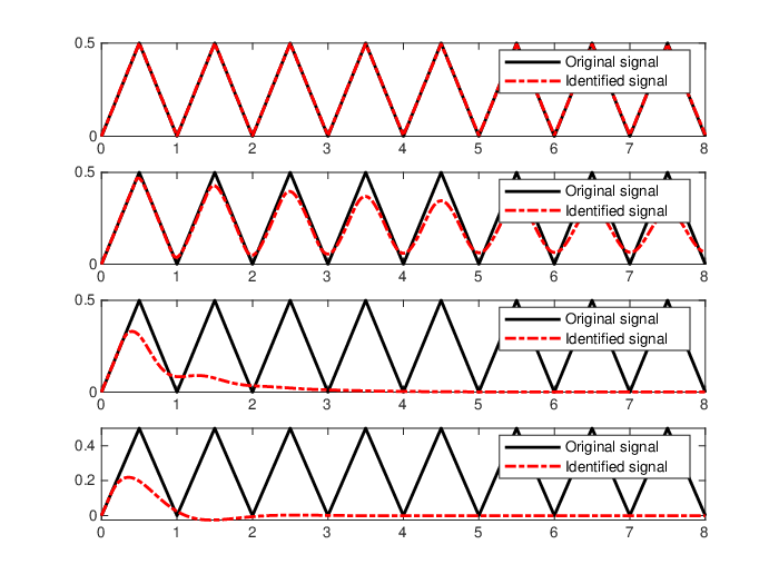
The identified signals for different values of the lag parameter LL are shown in figure 1.

Refer to caption
Figure 1. Identified signals for different lag values. L=17L=17 (top first row). L=16L=16 (second row). L=10L=10 (third row). L=5L=5 (bottom row).

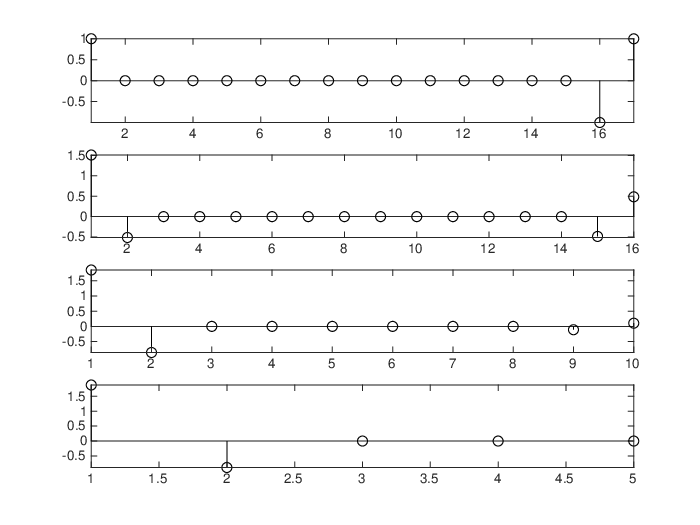
The ckc_{k} coefficients corresponding to the models identified for different values of the lag parameter LL are shown in figure 2.

Refer to caption
Figure 2. Identified coefficients for different lag values. L=17L=17 (top first row). L=16L=16 (second row). L=10L=10 (third row). L=5L=5 (bottom).

The root mean square error R​M​S​ERMSE corresponding to different values of the lag parameter LL are documented in table 1.

Lag value LL RMSE
17 0.002848195208845
16 0.067357195429571
10 0.265912048561782
5 0.279715847089058
Table 1. Root mean square errors corresponding to each lag value.

The computational setting used for this example is documented in the program Example1.m in [31]. For each lag value the corresponding model parameters were computed using program SpSolver.m in [31] based on algorithm 1, with the same tolerance δ>0\delta>0, in order to expose the potential topologically controlled approximation obstruction identified by the number drkδ,G1​(Σ~70)\mathrm{drk}_{\delta,G_{1}}(\tilde{\Sigma}_{70}).

As a consequence of theorem 4.3 and the previous observations, it can be seen that given a finite group GN⊂𝕌⁡(n)G_{N}\subset\mathbb{U}(n) and a sample ΣT={xt}t=1T\Sigma_{T}=\{x_{t}\}_{t=1}^{T} from a time series {xt}t≥1⊂ℂn\{x_{t}\}_{t\geq 1}\subset\mathbb{C}^{n} of a GNG_{N}-equivariant system (Σ,𝒯)(\Sigma,\mathscr{T}), if the number L^=degδ,GN​(ΣT)\hat{L}=\mathrm{deg}_{\delta,G_{N}}(\Sigma_{T}) is positive, we can use this number to estimate a necessary condition for the computability of a sparse solution to the problem

𝐇L,0⊤AT⊤≈δ𝐇L,1⊤\displaystyle\mathbf{H}_{L,0}^{\top}A_{T}^{\top}\approx_{\delta}\mathbf{H}_{L,1}^{\top}

where 𝐇L,k=ℋL​(Σk,GN)\mathbf{H}_{L,k}=\mathscr{H}_{L}\left(\Sigma_{k},G_{N}\right) for k=0,1k=0,1, with Σ0={xt}t=1T−1\Sigma_{0}=\{x_{t}\}_{t=1}^{T-1} and Σ1={xt}t=2T\Sigma_{1}=\{x_{t}\}_{t=2}^{T}. In particular, when L^=degδ,GN​(ΣT)\hat{L}=\mathrm{deg}_{\delta,G_{N}}(\Sigma_{T}) is positive, the lag value L=L^L=\hat{L} would provide a good starting point for an adaptive sparse system identification method, if the prediction error is still not small enough for the lag value L=L^L=\hat{L}, a controlling algorithm can keep increasing the value of the lag parameter until the prediction error is reached or some prescribed bound for the lag value is attained. For the experiments documented in this article, we have used standard scalar signal autocorrelation techniques to estimate admissible bounds for the lag values, in the Sparse Dynamical System Identification (SDSI) toolset available in [31] these ideas are implemented in the Matlab program LagEstimate.m based on the Matlab function xcorr.m.

The results and ideas presented in this section can be translated into sparse identification algorithms like algorithm 2.

4.2. Sparse parameter identification for finite difference models

Let us write ðh,k\eth_{h,k} to denote the finite difference representation of the time differentiation operator ∂t\partial_{t} with approximation order kk and uniform time partition size hh. Given a dictionary of dynamic variables u1,…,umu_{1},\ldots,u_{m}, a function f:(ℂn)m→(ℂn)pf:(\mathbb{C}^{n})^{m}\to(\mathbb{C}^{n})^{p} and time series samples {uj​(k)}k=1N⊂ℂn\{u_{j}(k)\}_{k=1}^{N}\subset\mathbb{C}^{n} corresponding to each dynamic variable, let us write VN​(f)​(𝐮)V_{N}(f)(\mathbf{u}) to denote the expression.

VN​(f)​(𝐮)\displaystyle V_{N}(f)(\mathbf{u}) =[f⁡(u1​(1),…,um​(1))f⁡(u1​(N),…,um​(N))]\displaystyle=\begin{bmatrix}f(u_{1}(1),\ldots,u_{m}(1))\\ \vdots\\ f(u_{1}(N),\ldots,u_{m}(N))\end{bmatrix}

In this section, given δ>0\delta>0 we will consider the approximate sparse identification problems of the form

(21) [||ð^h,k1​(u^1)⋯ð^h,km​(u^m)||]≈δ[||VN​(f1)​(𝐮)⋯VN​(fM)​(𝐮)||]𝐂,\displaystyle\begin{bmatrix}|&&|\\ \hat{\eth}_{h,k}^{1}(\hat{u}_{1})&\cdots&\hat{\eth}_{h,k}^{m}(\hat{u}_{m})\\ |&&|\end{bmatrix}\approx_{\delta}\begin{bmatrix}|&&|\\ V_{N}(f_{1})(\mathbf{u})&\cdots&V_{N}(f_{M})(\mathbf{u})\\ |&&|\end{bmatrix}\mathbf{C},

where ð^k,h1,…,ð^k,hm\hat{\eth}_{k,h}^{1},\ldots,\hat{\eth}_{k,h}^{m} denote finite difference operators based on ðk,h\eth_{k,h} with some additional specifications determined by the geometric or physical configuration of the system under study, and for each 1≤k≤m1\leq k\leq m, u^k=VN​(pk)​(𝐮)\hat{u}_{k}=V_{N}(p_{k})(\mathbf{u}) for pkp_{k} determined by the expression pk​(x1,…,xm)=xkp_{k}(x_{1},\ldots,x_{m})=x_{k}, and where each function fj:(ℂn)mj→(ℂn)pjf_{j}:(\mathbb{C}^{n})^{m_{j}}\to(\mathbb{C}^{n})^{p_{j}} is given for j=1,…,Mj=1,\ldots,M.

By applying theorem 3.6 to (21) we obtain the following solvability result.

Corollary 4.6.

Given δ>0\delta>0 and a problem of the form (21). If we set

r=rkδ​([||VN​(f1)​(𝐮)⋯VN​(fM)​(𝐮)||])\displaystyle r=\mathrm{rk}_{\delta}\left(\begin{bmatrix}|&&|\\ V_{N}(f_{1})(\mathbf{u})&\cdots&V_{N}(f_{M})(\mathbf{u})\\ |&&|\end{bmatrix}\right)

and if r>0r>0 then, there is a solution 𝐂\mathbf{C} to the problem (21) with at most r​∑k=1Mpkr\sum_{k=1}^{M}p_{k} nonzero entries.

Proof.

This is a direct application of theorem 3.6 to problem (21). ∎

Once an approximate sparse solution 𝐂\mathbf{C} to the problem (21) has been computed, one can apply numerical time integration methods to the continuous-time approximate representation of (21) determined by the expression

[||∂t(u^1)⋯∂t(u^m)||]=[||f1​(𝐮)⋯fM​(𝐮)||]​𝐂,\displaystyle\begin{bmatrix}|&&|\\ \partial_{t}(\hat{u}_{1})&\cdots&\partial_{t}(\hat{u}_{m})\\ |&&|\end{bmatrix}=\begin{bmatrix}|&&|\\ f_{1}(\mathbf{u})&\cdots&f_{M}(\mathbf{u})\\ |&&|\end{bmatrix}\mathbf{C},

with fj​(𝐮)=fj​(u1,…,um)f_{j}(\mathbf{u})=f_{j}(u_{1},\dots,u_{m}), in order to obtain a collection 𝒯1,…,𝒯m\mathscr{T}_{1},\ldots,\mathscr{T}_{m} of transition operators that approximately satisfy the equations:

uj​(k+1)=𝒯j​(u1​(k),…,um​(k))\displaystyle u_{j}(k+1)=\mathscr{T}_{j}(u_{1}(k),\ldots,u_{m}(k))

for each j=1,…,mj=1,\ldots,m, and each discrete time index k≥1k\geq 1.

5. Computational Methods

5.1. Algorithms

One of the purposes of this project is to provide sparse dynamical system identification (SDSI) tools that can be used to build collaborative frameworks of theoretical and computational methods that can be applied in a multidisciplinary context where adaptive approximate system identification is required. An example of the aforementioned collaborative frameworks can be described by the automaton illustrated in figure 3.

DDstartMMPP110,20,2002211112200
Figure 3. Finite-state automaton description of generic SDSI processes.

The blocks DD, MM and PP of the system 3 correspond to the data processing, model computation and predictive simulation stages of a generic sparse system identification process, respectively, while the labels 00, 11 and 22 correspond to the states computation in progress, computation completed and more data are required, respectively.

In this document we focus on the sparse linear least squares solver algorithms and approximate topological invariants in the form of easily computable numbers, that can be used in the modeling block MM of the automaton 3 for sparse model identification. Among other cases, the control signals for automata like 3 can be provided by an expert interested on the dynamics identification of some particular system, or by an artificially intelligent control system designed to build digital twins for a given system or process in some industrial environment. Although the programs in [31] can be used, adapted or modified to work in any of the two cases previously considered, the programs and examples included as part of the work reported in this document are written with the first case in mind. The artificially intelligent schemes will be further explored in the future.

Although the results in this document focus on sparse model identification, besides the programs corresponding to sparse linear least squares solvers and approximate degree and rank identifiers based on the results in §3 and §4, respectively, some programs for data reading and writing, synthetic signals generation, and predictive simulation are also include as part of the SDSI toolset available in [31].

5.1.1. Sparse linear least squares solver algorithm

As an application of the results and ideas presented in §3 one can obtain a prototypical sparse linear least squares solver algorithm like algorithm 1.

Algorithm 1 SLRSolver: Sparse linear least squares solver algorithm
 Data:    A∈ℂm×nA\in\mathbb{C}^{m\times n}, Y∈ℂm×pY\in\mathbb{C}^{m\times p}, δ>0\delta>0, N∈ℤ+N\in\mathbb{Z}^{+}, ε>0\varepsilon>0
 Result:    X=𝐒𝐋𝐑𝐒𝐨𝐥𝐯𝐞𝐫⁡(A,Y,δ,N,ε)X=\mathbf{SLRSolver}(A,Y,\delta,N,\varepsilon)
  1. (1)

    Compute economy-sized SVD U​S​V=AUSV=A 

  2. (2)

    Set s=min⁡{m,n}s=\min\{m,n\} 

  3. (3)

    Set r=rkδ​(A)r=\mathrm{rk}_{\delta}(A) 

  4. (4)

    Set Uδ=∑j=1rU​e^j,s​e^j,s∗U_{\delta}=\sum_{j=1}^{r}U\hat{e}_{j,s}\hat{e}_{j,s}^{\ast} 

  5. (5)

    Set Tδ=∑j=1r(e^j,s∗​S​e^j,s)−1​e^j,s​e^j,s∗T_{\delta}=\sum_{j=1}^{r}(\hat{e}_{j,s}^{\ast}S\hat{e}_{j,s})^{-1}\hat{e}_{j,s}\hat{e}_{j,s}^{\ast} 

  6. (6)

    Set Vδ=∑j=1re^j,s​e^j,s∗​VV_{\delta}=\sum_{j=1}^{r}\hat{e}_{j,s}\hat{e}_{j,s}^{\ast}V 

  7. (7)

    Set A^=Uδ∗​A\hat{A}=U_{\delta}^{\ast}A 

  8. (8)

    Set Y^=Uδ∗​Y\hat{Y}=U_{\delta}^{\ast}Y 

  9. (9)

    Set X0=Vδ∗​Tδ​Y^X_{0}=V_{\delta}^{\ast}T_{\delta}\hat{Y} 

  10. (10)

    for j=1,…,pj=1,\ldots,p do

  11. (11)

    Set K=1K=1 

  12. (12)

    Set error=1+δ\mathrm{error}=1+\delta 

  13. (13)

    Set c=X0​e^j,pc=X_{0}\hat{e}_{j,p}

  14. (14)

    Set x0=cx_{0}=c

  15. (15)

    Set c^=[c^1⋯c^n]⊤=[|e^1,n∗​c|⋯|e^n,n∗​c|]⊤\hat{c}=\begin{bmatrix}\hat{c}_{1}&\cdots&\hat{c}_{n}\end{bmatrix}^{\top}=\begin{bmatrix}|\hat{e}_{1,n}^{\ast}c|&\cdots&|\hat{e}_{n,n}^{\ast}c|\end{bmatrix}^{\top} 

  16. (16)

    Compute permutation σ:{1,…,n}→{1,…,n}\sigma:\{1,\ldots,n\}\to\{1,\ldots,n\} such that: c^σ⁡(1)≥c^σ⁡(2)≥⋯≥c^σ⁡(n)\hat{c}_{\sigma(1)}\geq\hat{c}_{\sigma(2)}\geq\cdots\geq\hat{c}_{\sigma(n)}

  17. (17)

    Set N0=max⁡{∑j=1nHε​(c^σ⁡(j)),1}N_{0}=\max\left\{\sum_{j=1}^{n}H_{\varepsilon}\left(\hat{c}_{\sigma(j)}\right),1\right\} 

  18. (18)

    while K≤NK\leq N and error>δ\mathrm{error}>\delta do

  19. (19)

    Set x=𝟎n,1x=\mathbf{0}_{n,1} 

  20. (20)

    Set A0=∑j=1N0A^​e^σ⁡(j),n​e^j,N0∗A_{0}=\sum_{j=1}^{N_{0}}\hat{A}\hat{e}_{\sigma(j),n}\hat{e}_{j,N_{0}}^{\ast}

  21. (21)

    Solve c=arg⁡minc~∈ℂN0​‖A0​c~−Y^​e^j,p‖c=\arg\min_{\tilde{c}\in\mathbb{C}^{N_{0}}}\|A_{0}\tilde{c}-\hat{Y}\hat{e}_{j,p}\| 

  22. (22)
  23. (23)

    for k=1,…,N0k=1,\ldots,N_{0} do

  24. (24)

    Set xσ⁡(k)=e^k,N0∗​cx_{\sigma(k)}=\hat{e}_{k,N_{0}}^{\ast}c 

  25. (25)

    end for 

  26. (26)

    Set error=‖x−x0‖∞\mathrm{error}=\|x-x_{0}\|_{\infty} 

  27. (27)

    Set x0=xx_{0}=x 

  28. (28)

    Set c^=[c^1⋯c^n]⊤=[|e^1,n∗​x|⋯|e^n,n∗​x|]⊤\hat{c}=\begin{bmatrix}\hat{c}_{1}&\cdots&\hat{c}_{n}\end{bmatrix}^{\top}=\begin{bmatrix}|\hat{e}_{1,n}^{\ast}x|&\cdots&|\hat{e}_{n,n}^{\ast}x|\end{bmatrix}^{\top} 

  29. (29)

    Compute permutation σ:{1,…,n}→{1,…,n}\sigma:\{1,\ldots,n\}\to\{1,\ldots,n\} such that: c^σ⁡(1)≥c^σ⁡(2)≥⋯≥c^σ⁡(n)\hat{c}_{\sigma(1)}\geq\hat{c}_{\sigma(2)}\geq\cdots\geq\hat{c}_{\sigma(n)}

  30. (30)

    Set N0=max⁡{∑j=1nHε​(c^σ⁡(j)),1}N_{0}=\max\left\{\sum_{j=1}^{n}H_{\varepsilon}\left(\hat{c}_{\sigma(j)}\right),1\right\}

  31. (31)

    Set K=K+1K=K+1 

  32. (32)

    end while

  33. (33)

    Set xj=xx_{j}=x 

  34. (34)

    end for

  35. (35)

    Set X=[|||x1x2⋯xp|||]X=\begin{bmatrix}|&|&&|\\ x_{1}&x_{2}&\cdots&x_{p}\\ |&|&&|\end{bmatrix} 

 return XX

The least squares problems c=arg⁡minc^∈ℂK​‖A^​c^−y‖c=\arg\min_{\hat{c}\in\mathbb{C}^{K}}\|\hat{A}\hat{c}-y\| to be solved as part of the process corresponding to algorithm 1 can be solved with any efficient least squares solver available in the language or program where the sparse linear least squares solver algorithm is implemented. For the Matlab and Julia implementations of algorithm 1 written as part of this research project the backslash "\\backslash" operator is used, and for the Python version of algorithm 1 the function lstsq is implemented.

5.1.2. Sparse time series model identification algorithm

Given a time series {xt}t≥1\{x_{t}\}_{t\geq 1} of a system (Σ,𝒯)(\Sigma,\mathscr{T}) with transition operator 𝒯\mathscr{T} to be identified, we can approach the computation of local approximations of 𝒯\mathscr{T} based on a structured data sample ΣT={xt}t=1T⊂Σ\Sigma_{T}=\{x_{t}\}_{t=1}^{T}\subset\Sigma using the prototypical algorithm outlined in algorithm 2.

Algorithm 2 SDSI: algorithm for sparse dynamical system identification
 Data:    GN⊂𝕌⁡(n)G_{N}\subset\mathbb{U}(n), Σ^T={xt}t=1T⊂ℂn\hat{\Sigma}_{T}=\{x_{t}\}_{t=1}^{T}\subset\mathbb{C}^{n}, L∈ℤ+L\in\mathbb{Z}^{+}, δ>0,ε>0\delta>0,\varepsilon>0
 Result:    (𝒫L,A^T,AT,X1)=𝐒𝐃𝐒𝐈⁡(GN,Σ^T,L,δ,ε)(\mathscr{P}_{L},\hat{A}_{T},A_{T},X_{1})=\mathbf{SDSI}(G_{N},\hat{\Sigma}_{T},L,\delta,\varepsilon)
  1. (1)

    Compute L=max⁡{degδ,GN​(Σ^T),L}L=\max\{\mathrm{deg}_{\delta,G_{N}}(\hat{\Sigma}_{T}),L\} 

  2. (2)

    Set Σ^0={xt}t=1T−1\hat{\Sigma}_{0}=\{x_{t}\}_{t=1}^{T-1}, Σ^1={xt}t=2T\hat{\Sigma}_{1}=\{x_{t}\}_{t=2}^{T} 

  3. (3)

    Set 𝐇L,k=ℋL​(Σ^k,GN)\mathbf{H}_{L,k}=\mathscr{H}_{L}(\hat{\Sigma}_{k},G_{N}), k=0,1k=0,1 

  4. (4)

    Solve 𝐇L,0⊤C≈δ𝐇L,1⊤\mathbf{H}_{L,0}^{\top}C\approx_{\delta}\mathbf{H}_{L,1}^{\top} applying algorithm 1 with the setting C=𝐒𝐋𝐑𝐒𝐨𝐥𝐯𝐞𝐫⁡(𝐇L,0⊤,𝐇L,1⊤,δ,n​L,ε)C=\mathbf{SLRSolver}(\mathbf{H}_{L,0}^{\top},\mathbf{H}_{L,1}^{\top},\delta,nL,\varepsilon) 

  5. (5)

    Set A^T=C⊤\hat{A}_{T}=C^{\top}  

  6. (6)

    Set AT=1N​∑j=1N(IL⊗gj∗)​A^T​(IL⊗gj)A_{T}=\frac{1}{N}\sum_{j=1}^{N}\left(I_{L}\otimes g_{j}^{\ast}\right)\hat{A}_{T}\left(I_{L}\otimes g_{j}\right)  

  7. (7)

    Set X1=[x1⊤⋯xL⊤]⊤X_{1}=\left[x_{1}^{\top}\>\cdots\>x_{L}^{\top}\right]^{\top} 

  8. (8)

    Set 𝒫L=e^1,L⊤⊗In\mathscr{P}_{L}=\hat{e}_{1,L}^{\top}\otimes I_{n} 

 return (𝒫L,A^T,AT,X1)(\mathscr{P}_{L},\hat{A}_{T},A_{T},X_{1})

For the study reported in this document, when the time series data ΣT={xt}t=1T⊂ℂn\Sigma_{T}=\{x_{t}\}_{t=1}^{T}\subset\mathbb{C}^{n} of a given system (Σ,𝒯)(\Sigma,\mathscr{T}) with transition operator 𝒯\mathscr{T} to be identified, is not uniformly sampled in time, the sample ΣT\Sigma_{T} is preprocessed applying local spline interpolation methods to obtain a uniform in time estimate Σ~T={x~t}t=1T⊂ℂn\tilde{\Sigma}_{T}=\{\tilde{x}_{t}\}_{t=1}^{T}\subset\mathbb{C}^{n} for ΣT\Sigma_{T}. The Matlab program DataSpliner.m is an example of a computational implementation of this interpolation procedure and is included as part of the programs in the SDSI toolset available at [31].

Given a finite group GN⊂𝕌⁡(n)G_{N}\subset\mathbb{U}(n), a GNG_{N}-equivariant system (Σ,𝒯)(\Sigma,\mathscr{T}) and a structured data sample ΣT⊂Σ\Sigma_{T}\subset\Sigma, if the elements 𝒫,A^,A,X1\mathscr{P},\hat{A},A,X_{1} are computed using algorithm 2 with the setting (𝒫,A^,A,X1)=𝐒𝐃𝐒𝐈⁡(GN,Σ^T,L,δ,ε)(\mathscr{P},\hat{A},A,X_{1})=\mathbf{SDSI}(G_{N},\hat{\Sigma}_{T},L,\delta,\varepsilon) for some suitable δ,ε>0\delta,\varepsilon>0, one can build two predictive models 𝐏A^,𝐏A\mathbf{P}_{\hat{A}},\mathbf{P}_{A} for the time evolution of the system, determined by the recurrence relation xt+1=𝒯⁡(xt),t≥1x_{t+1}=\mathscr{T}(x_{t}),t\geq 1, using schemes of the form 𝐏A^​(t)=𝒫​A^t​X1\mathbf{P}_{\hat{A}}(t)=\mathscr{P}\hat{A}^{t}X_{1} and 𝐏A​(t)=𝒫​At​X1\mathbf{P}_{A}(t)=\mathscr{P}A^{t}X_{1} for t≥1t\geq 1.

5.2. Numerical Simulations

In this section we will present some numerical simulations computed using the SDSI toolset available in [31], that was developed as part of this project, the toolset consists of a collection of programs written in Matlab, Julia and Python that can be used for sparse identification and numerical simulation of dynamical systems.

The numerical experiments documented in this section were performed with Matlab R2021a (9.10.0. 1602886) 64-bit (glnxa64), Julia 1.6.0, Python 3.8 and Netgen/NGSolve 6.2. Some Matlab and Python Netgen/NGSolve programs were used to generate synthetic data used for some of the system identification processes. All the programs written for synthetic data generation and sparse model identification as part of this project are available at [31].

The numerical simulations reported in this section were computed on a Linux Ubuntu Server 20.04 PC equiped with an Intel Xeon E3-1225 v5 (8M Cache, 3.30 GHz) processor and with 40GB RAM.

5.2.1. Sparse identification of a finite difference model for the nonlinear Schrödinger equation in the finite line

In this section a finite difference model corresponding to a nonlinear Schrödinger equation of the form

(22) i​∂tw+∂x2w+q​|w|2​w=0i\partial_{t}w+\partial_{x}^{2}w+q|w|^{2}w=0

for x∈[−20,20]x\in[-20,20] and t≥0t\geq 0, will be approximately identified. The synthetic signals corresponding to the csv data file NLSEqData.csv that will be used for system identification have been computed using a fourth order Runge-Kutta scheme to integrate the corresponding second order in space finite difference discretization of (22), with initial conditions and homogeneous Dirichlet boundary conditions based on the configuration used by Ramos and Villatoro in [24] using the Matlab program NLSchrodinger1DRK.m in [31]. The amplitudes corresponding to the dynamical behavior data Σ4401={𝐰⁡(t)}t=14401⊂ℂ161\Sigma_{4401}=\{\mathbf{w}(t)\}_{t=1}^{4401}\subset\mathbb{C}^{161} saved in file NLSEqData.csv are visualized in figure 4.

Refer to caption
Figure 4. Amplitudes corresponding to an approximation of a travelling wave solution to equation (22).

Let us consider the finite difference model

(23) i​ð^ht,4​𝐰+𝐃hx,2​𝐰+q​|𝐰|2​𝐰=0i\hat{\eth}_{h_{t},4}\mathbf{w}+\mathbf{D}_{h_{x},2}\mathbf{w}+q|\mathbf{w}|^{2}\mathbf{w}=0

corresponding to (22), where the operation ð^ht,4​𝐰​(t)\hat{\eth}_{h_{t},4}\mathbf{w}(t) is defined for an arbitrary differentiable function t↦𝐰⁡(t)=[w1​(t)⋯w161​(t)]⊤∈ℂ161t\mapsto\mathbf{w}(t)=\begin{bmatrix}w_{1}(t)&\cdots&w_{161}(t)\end{bmatrix}^{\top}\in\mathbb{C}^{161} by the expression

ð^ht,4​𝐰​(t)=[0ðht,4​w2​(t)⋯ðht,4​w160​(t)0]⊤.\displaystyle\hat{\eth}_{h_{t},4}\mathbf{w}(t)=\begin{bmatrix}0&\eth_{h_{t},4}w_{2}(t)&\cdots&\eth_{h_{t},4}w_{160}(t)&0\end{bmatrix}^{\top}.

The choice of fourth order approximations ðht,4​wk​(t)\eth_{h_{t},4}w_{k}(t) of each derivative ∂twk​(t)\partial_{t}w_{k}(t) for 2≤k≤1602\leq k\leq 160, is based on the fact that the synthetic data Σ4401\Sigma_{4401} recorded in NLSEqData.csv were computed using a fourth order Runge-Kutta scheme for time integration.

We will apply algorithm 1 along the lines of corollary 4.6 to identify model (23), using a dictionary of 203203 functions fj:ℂ161→ℂ161f_{j}:\mathbb{C}^{161}\to\mathbb{C}^{161} defined in terms of a generic 𝐮=[uj]∈ℂ161\mathbf{u}=\begin{bmatrix}u_{j}\end{bmatrix}\in\mathbb{C}^{161} by the following expressions

f1​(𝐮)\displaystyle f_{1}(\mathbf{u}) =[0u2u3⋯u1600]⊤,\displaystyle=\begin{bmatrix}0&u_{2}&u_{3}&\cdots&u_{160}&0\end{bmatrix}^{\top},
f2​(𝐮)\displaystyle f_{2}(\mathbf{u}) =[00u2u3⋯u1590]⊤\displaystyle=\begin{bmatrix}0&0&u_{2}&u_{3}&\cdots&u_{159}&0\end{bmatrix}^{\top}
f3​(𝐮)\displaystyle f_{3}(\mathbf{u}) =[0u3u4⋯u16000]⊤\displaystyle=\begin{bmatrix}0&u_{3}&u_{4}&\cdots&u_{160}&0&0\end{bmatrix}^{\top}
f4​(𝐮)\displaystyle f_{4}(\mathbf{u}) =[0|u2|​u2|u3|​u3⋯|u160|​u1600]⊤,\displaystyle=\begin{bmatrix}0&|u_{2}|u_{2}&|u_{3}|u_{3}&\cdots&|u_{160}|u_{160}&0\end{bmatrix}^{\top},
f5​(𝐮)\displaystyle f_{5}(\mathbf{u}) =[0|u2|2​u2|u3|2​u3⋯|u160|2​u1600]⊤,\displaystyle=\begin{bmatrix}0&|u_{2}|^{2}u_{2}&|u_{3}|^{2}u_{3}&\cdots&|u_{160}|^{2}u_{160}&0\end{bmatrix}^{\top},
f203​(𝐮)\displaystyle f_{203}(\mathbf{u}) =[0|u2|200​u2|u3|200​u3⋯|u160|200​u1600]⊤.\displaystyle=\begin{bmatrix}0&|u_{2}|^{200}u_{2}&|u_{3}|^{200}u_{3}&\cdots&|u_{160}|^{200}u_{160}&0\end{bmatrix}^{\top}.

Since the synthetic data Σ4401\Sigma_{4401} was generated using Runge-Kutta approximation of a second order finite difference discretization of (22), there is some numerical noise induced in the synthetic signal due to floating point errors, in addition, for this experiment some pseudorandom noise with 𝒪⁡(10−6)\mathcal{O}(10^{-6}) is added to the reference data Σ4401\Sigma_{4401} to obtain a noisier version Σ~4401\tilde{\Sigma}_{4401} of Σ4401\Sigma_{4401} that has been recorded in [31] as NoisyNLSEqData.csv for future references.

Some reference data corresponding to the amplitude |w||w| of ww together with the predictions computed with the model that has been identified using the sparse solver of the SDSI toolset are visualized in figure 5.

Refer to caption
Figure 5. Reference data amplitudes |w⁡(t)||w(t)| (top). Predicted values of the amplitudes |wp​(t)||w_{p}(t)| computed with SDSI model identifier (bottom).

The sparse identification of the signal data Σ4401\Sigma_{4401} corresponding to the discretization (23) of (22) was also computed using standard SINDy and Douglas-Rachford sparse solvers as presented and implemented in [6] and [27]. The absolute prediction errors corresponding to the SDSI, SINDy and Douglas-Rachford solvers in the ℓ∞\ell_{\infty}-norm are shown in figure 6.

Refer to caption
Figure 6. Prediction errors in the ℓ∞\ell_{\infty}-norm.

The running times are documented in the table 2.

Method Running Time (seconds)
SDSI 0.122988
SINDy 0.258558
Douglas-Rachford 286.864170
Table 2. Running time of the sparse identification methods

Let us write wkw_{k} to denote the kk-component of the state vector 𝐰⁡(t)∈ℂ161\mathbf{w}(t)\in\mathbb{C}^{161} determined by the expression wk=w⁡(−20+(k−1)​hx,t​h)w_{k}=w(-20+(k-1)h_{x},th) for hx=1/4h_{x}=1/4 and h=1/10h=1/10. The corresponding semi-discrete model will be

i​w˙k\displaystyle i\dot{w}_{k} =−32​wk+16​wk+1+16​wk−1+|wk|2​wk,2≤k≤160\displaystyle=-32w_{k}+16w_{k+1}+16w_{k-1}+|w_{k}|^{2}w_{k},2\leq k\leq 160

with w1=w161=0w_{1}=w_{161}=0. The semi-discrete models identified by each method based on a training set of 3535 samples Σ~35={𝐰~​(1),…,𝐰~​(35)}⊂Σ~4401\tilde{\Sigma}_{35}=\{\tilde{\mathbf{w}}(1),\ldots,\tilde{\mathbf{w}}(35)\}\subset\tilde{\Sigma}_{4401} for each 2≤k≤1602\leq k\leq 160 are documented in table 3, for every model in the table w1=w161=0w_{1}=w_{161}=0.

Method Indentified Model
SDSI i​w˙k=(−31.8766−0.0276​i)​wk+(15.9414+0.0211​i)​wk+1+(15.9381+0.0059​i)​wk−1+(0.9962+0.0008​i)​|wk|2​wk\!\begin{aligned} i\dot{w}_{k}&=(-31.8766-0.0276i)w_{k}+(15.9414+0.0211i)w_{k+1}\\ &+(15.9381+0.0059i)w_{k-1}+(0.9962+0.0008i)|w_{k}|^{2}w_{k}\end{aligned}
SINDy i​w˙k=(−31.8705−0.0646​i)​wk+(15.9408+0.0390​i)​wk+1+(15.9330+0.0231​i)​wk−1+(−0.0340+0.1333​i)​|wk|​wk+(2.8996−6.5725​i)​|wk|2​wk+(−52.3400+160.4634​i)​|wk|3​wk+(790.9174−2.2437×10³)​|wk|4​wk+(25​more​terms)\!\begin{aligned} i\dot{w}_{k}&=(-31.8705-0.0646i)w_{k}+(15.9408+0.0390i)w_{k+1}\\ &+(15.9330+0.0231i)w_{k-1}+(-0.0340+0.1333i)|w_{k}|w_{k}\\ &+(2.8996-6.5725i)|w_{k}|^{2}w_{k}+(-52.3400+160.4634i)|w_{k}|^{3}w_{k}\\ &+(790.9174-2.2437\times 10^{3})|w_{k}|^{4}w_{k}+(25\>\>\mathrm{more}\>\>\mathrm{terms})\end{aligned}
Douglas-Rachford i​w˙k=(−29.0860−0.0599​i)​wk+(14.5809+0.2070​i)​wk+1+(14.5735−0.1480​i)​wk−1+(0.9042+0.0012​i)​|wk|2​wk+(0.0045−0.0002​i)​|wk|3​wk\!\begin{aligned} i\dot{w}_{k}&=(-29.0860-0.0599i)w_{k}+(14.5809+0.2070i)w_{k+1}\\ &+(14.5735-0.1480i)w_{k-1}+(0.9042+0.0012i)|w_{k}|^{2}w_{k}\\ &+(0.0045-0.0002i)|w_{k}|^{3}w_{k}\end{aligned}
Table 3. Model Indentified by each method

The computational setting used for this experiment is documented in the Matlab program
NLSESpModelID.m in [31] that can be used to replicate this experiment.

5.2.2. Sparse identification of a network of Duffing oscillators with symmetries

In this section a network of three coupled Duffing oscillators with the following configuration

x˙i=yi,i∈{1,2,3}\displaystyle\dot{x}_{i}=y_{i},\>\>i\in\{1,2,3\}
y˙i=σ​yj−xi​(β+α2​xi)+∑i​jηi​j​(xi−xj),i∈{1,2,3}\displaystyle\dot{y}_{i}=\sigma y_{j}-x_{i}(\beta+\alpha^{2}x_{i})+\sum_{ij}\eta_{ij}(x_{i}-x_{j}),\>\>i\in\{1,2,3\}
x1​(0)=8,x2​(0)=7,x3​(0)=4,\displaystyle x_{1}(0)=8,x_{2}(0)=7,x_{3}(0)=4,
(24) y1​(0)=15,y2​(0)=14,y3​(0)=9\displaystyle y_{1}(0)=15,y_{2}(0)=14,y_{3}(0)=9

is identified, for α=1,β=−36,σ=0\alpha=1,\beta=-36,\sigma=0 and with all the coupling strengths ηi​j\eta_{ij} equal to 1/51/5. The configuration of these experiment is based on the example II.2 considered in [26], an important part of the motivation for the study of this types of networks of oscillators comes from interesting applications in engineering and biological cybernetics like the ones presented in [10], [25] and [9]. Since all the coupling strengths ηi​j\eta_{ij} are equal to 1/51/5, as stablished in [26] the system (24) will be D3D_{3}-equivariant, and for the configuration used for this experiment, the matrix representation of the corresponding group of symmetries D3=⟨r,κ|r3=κ2=e,κrκ=r−1⟩D_{3}=\langle r,\kappa|r^{3}=\kappa^{2}=e,\kappa r\kappa=r^{-1}\rangle is determined by the following assignments.

r\displaystyle r ↦rρ=I2⊗[010001100]\displaystyle\mapsto r_{\rho}=I_{2}\otimes\begin{bmatrix}0&1&0\\ 0&0&1\\ 1&0&0\end{bmatrix}
κ\displaystyle\kappa ↦κρ=I2⊗[100001010]\displaystyle\mapsto\kappa_{\rho}=I_{2}\otimes\begin{bmatrix}1&0&0\\ 0&0&1\\ 0&1&0\end{bmatrix}

The synthetic signal used for sparse identification of (24) was computed with an adaptive fourth order Runge-Kutta scheme. The model was trained using the dictionary

f1​(x1,x2,x3,y1,y2,y3)\displaystyle f_{1}(x_{1},x_{2},x_{3},y_{1},y_{2},y_{3}) =(x1,x2,x3,y1,y2,y3)\displaystyle=(x_{1},x_{2},x_{3},y_{1},y_{2},y_{3})
f2​(x1,x2,x3,y1,y2,y3)\displaystyle f_{2}(x_{1},x_{2},x_{3},y_{1},y_{2},y_{3}) =(x12,x22,x32)\displaystyle=(x_{1}^{2},x_{2}^{2},x_{3}^{2})
f3​(x1,x2,x3,y1,y2,y3)\displaystyle f_{3}(x_{1},x_{2},x_{3},y_{1},y_{2},y_{3}) =(x13,x23,x33)\displaystyle=(x_{1}^{3},x_{2}^{3},x_{3}^{3})
f9​(x1,x2,x3,y1,y2,y3)\displaystyle f_{9}(x_{1},x_{2},x_{3},y_{1},y_{2},y_{3}) =(x19,x29,x39)\displaystyle=(x_{1}^{9},x_{2}^{9},x_{3}^{9})

with 20%20\% of the synthetic reference data.

The reference synthetic signal and the corresponding identified signals are illustrated in figure 7

Refer to caption
Figure 7. Synthetic reference position signals (top). Signals identified using SDSI sparse solver (middle). Signals identified using SINDy sparse solver (bottom).

The prediction errors ‖𝐱​(t)−𝐱p​(t)‖\|\mathbf{x}(t)-\mathbf{x}_{p}(t)\|, and the equivariance errors ‖F⁡(rρ​𝐱​(t))−rρ​F​(𝐱⁡(t))‖\|F(r_{\rho}\mathbf{x}(t))-r_{\rho}F(\mathbf{x}(t))\| and ‖F⁡(κρ​𝐱​(t))−κρ​F​(𝐱⁡(t))‖\|F(\kappa_{\rho}\mathbf{x}(t))-\kappa_{\rho}F(\mathbf{x}(t))\| of the identified right hand side FF for a model x˙=F⁡(x)\dot{x}=F(x) of the form (24), for each discrete time index tt are plotted in figure 8.

Refer to caption
Figure 8. Prediction errors (top). Equivariance errors for rρr_{\rho} (middle). Equivariance errors for κρ\kappa_{\rho} (bottom).

The models identified by each method are documented in tables 4 and 5.

Method Indentified Model
SDSI x˙1=0.999999992419860​y1,x˙2=0.999999992358200​y2,x˙3=0.999999992182884​y3,y˙1=36.399999678455494​x1−0.200001381665299​x2−0.199999513388808​x3−0.999999969696376​x12,y˙2=−0.199999469429072​x1+36.399998021632314​x2−0.199999719964769​x3−0.999999971061446​x22,y˙3=−0.199998908401240​x1−0.200001498693973​x2+36.399999282587004​x3−0.999999971862063​x32,\!\begin{aligned} \dot{x}_{1}&=0.999999992419860y_{1},\\ \dot{x}_{2}&=0.999999992358200y_{2},\\ \dot{x}_{3}&=0.999999992182884y_{3},\\ \dot{y}_{1}&=36.399999678455494x_{1}-0.200001381665299x_{2}-0.199999513388808x_{3}\\ &-0.999999969696376x_{1}^{2},\\ \dot{y}_{2}&=-0.199999469429072x_{1}+36.399998021632314x_{2}-0.199999719964769x_{3}\\ &-0.999999971061446x_{2}^{2},\\ \dot{y}_{3}&=-0.199998908401240x_{1}-0.200001498693973x_{2}+36.399999282587004x_{3}\\ &-0.999999971862063x_{3}^{2},\end{aligned}
Table 4. Model Indentified by SDSI.
Method Indentified Model
SINDy x˙1=0.999999992419860​y1,x˙2=0.999999992358200​y2,x˙3=0.999999992182883​y3,y˙1=36.399999678455423​x1−0.200001381665187​x2−0.199999513388848​x3−0.999999969696376​x12,y˙2=−0.199999469429017​x1+36.399998021632094​x2−0.199999719964673​x3−0.999999971061444​x22,y˙3=−0.199998908401247​x1−0.200001498693980​x2+36.399999282587018​x3−0.999999971862063​x32,\!\begin{aligned} \dot{x}_{1}&=0.999999992419860y_{1},\\ \dot{x}_{2}&=0.999999992358200y_{2},\\ \dot{x}_{3}&=0.999999992182883y_{3},\\ \dot{y}_{1}&=36.399999678455423x_{1}-0.200001381665187x_{2}-0.199999513388848x_{3}\\ &-0.999999969696376x_{1}^{2},\\ \dot{y}_{2}&=-0.199999469429017x_{1}+36.399998021632094x_{2}-0.199999719964673x_{3}\\ &-0.999999971061444x_{2}^{2},\\ \dot{y}_{3}&=-0.199998908401247x_{1}-0.200001498693980x_{2}+36.399999282587018x_{3}\\ &-0.999999971862063x_{3}^{2},\end{aligned}
Table 5. Model Indentified by SINDy.

The running times for the computation of each model are documented in table 6.

Method Running Time (seconds)
SDSI 0.0024070.002407
SINDy 0.0013760.001376
Table 6. Running times for the computation of the nonlinear model identifications.

Using the same data we can apply algorithm 2 to compute a local linear model approximant for the model 24. The identified signals computed using SDSI sparse solver are shown in figure 9 and the identified signals computed using SINDy sparse solver are shown in figure 10.

Refer to caption
Figure 9. Signal identification computed with SDSI for: x1x_{1} (top). x2x_{2} (middle). x3x_{3} (bottom).
Refer to caption
Figure 10. Signal identification computed with SINDy for: x1x_{1} (top). x2x_{2} (middle). x3x_{3} (bottom).

The sparsity patterns of the matrices of parameters identified by each method are shown in figure 11.

Refer to caption
Figure 11. Sparsity pattern of the matrix of parameters identified by: SDSI (left). SINDy (right).

Let us set r^ρ=IL⊗rρ\hat{r}_{\rho}=I_{L}\otimes r_{\rho} and κ^ρ=IL⊗κρ\hat{\kappa}_{\rho}=I_{L}\otimes\kappa_{\rho}. The numerical errors corresponding to the symmetry constraints imposed to the matrices of parameters are documented in table 7.

Method ‖r^ρ​AT−AT​r^ρ‖F\|\hat{r}_{\rho}A_{T}-A_{T}\hat{r}_{\rho}\|_{F} ‖κ^ρ​AT−AT​κ^ρ‖F\|\hat{\kappa}_{\rho}A_{T}-A_{T}\hat{\kappa}_{\rho}\|_{F}
SDSI 6.311151928321685×10−166.311151928321685\times 10^{-16} 00
SINDy 9.138315630890346×10−169.138315630890346\times 10^{-16} 00
Table 7. Numerical errors corresponding to the symmetry preserving constraints.

The root mean square errors corresponding to the variables considered for the local linear model approximants are documented in table 8, and the running times corresponding to the computation of the local linear model approximants are documented in table 9.

Variable RMSE (SDSI) RMSE (SINDy)
x1x_{1} 0.1534921694537910.153492169453791 0.1544971349583700.154497134958370
x2x_{2} 0.0322577126385610.032257712638561 0.0327399614113930.032739961411393
x3x_{3} 0.2271243938167120.227124393816712 0.2279943289813420.227994328981342
Table 8. Root mean square errors corresponding to each method and variable.
Method Running Time (seconds)
SDSI 0.0959870.095987
SINDy 0.4202930.420293
Table 9. Running times for the computation of the local linear model approximant.

The computational setting used for the experiments performed in this section is documented in the Matlab programs NLONetworkID.m and DuffingLTIModelID.m in [31] that can be used to replicate these experiments.

5.2.3. Sparse identification of a time series model for vortex shedding processes

Let us consider a Navier-Stokes nonlinear model of the form

∂u∂t+u⋅∇u−ν​Δ​u+∇p\displaystyle\frac{\partial{u}}{\partial{t}}+u\cdot\nabla u-\nu\Delta u+\nabla p =0\displaystyle=0
(25) ∇⋅u\displaystyle\nabla\cdot u =0\displaystyle=0

under suitable geometric configuration, initial and boundary conditions that lead to vortex shedding. For this experiment, the sparse model identification process is based on the synthetic data corresponding to a vortex shedding process recorded in the file GFUdata.csv, that is included in [31] as the compressed file GFUdata.zip, the synthetic data were generated using the program navierstokes-tcsi.py included in [31] that is based on the Netgen/Python program navierstokes.py developed by J. Schöberl as part of the work initiated with [29].

The time series model identification based on the data Σ502={ut}t=1502⊂ℝ53770\Sigma_{502}=\{u_{t}\}_{t=1}^{502}\subset\mathbb{R}^{53770} recorded in GFUdata.csv is performed with a computational implementation of algorithm 2 using the Matlab program NSIdentifier.m which estimates the number deg9×10−7,{I53770}​(Σ400)\mathrm{deg}_{9\times 10^{-7},\{I_{53770}\}}(\Sigma_{400}) obtaining the value deg9×10−7,{I53770}​(Σ400)=1\mathrm{deg}_{9\times 10^{-7},\{I_{53770}\}}(\Sigma_{400})=1, for this experiment we have that rkδ​(ℋ1​(Σ400))=354\mathrm{rk}_{\delta}(\mathscr{H}_{1}(\Sigma_{400}))=354, and the models are trained with the subsample Σ354={ut}t=1354⊂Σ400⊂Σ502\Sigma_{354}=\{u_{t}\}_{t=1}^{354}\subset\Sigma_{400}\subset\Sigma_{502}.

Since d=1d=1, the models can be computed using the reduced form

uk+1=ℋ1​(Σ353)​A353k​e^1,353,k≥1\displaystyle u_{k+1}=\mathscr{H}_{1}(\Sigma_{353})A_{353}^{k}\hat{e}_{1,353},\>\>k\geq 1

with Σ353={ut}t=1353\Sigma_{353}=\{u_{t}\}_{t=1}^{353}, and only a matrix of parameters A353A_{353} is left to be identified. The matrix of parameters will be identified using the sparse solver SpSolver.m from the SDSI toolset based on algorithm 1 and the sparse solver SINDy.m based on SINDy sparse least squares solver algorithm introduced in [6].

The sparsity patterns of the matrices of parameters identified by the Matlab programs SpSolver.m and SINDy.m are shown in figure 12.

Refer to caption
Figure 12. Sparsity patterns of matrices of parametres identified by: SINDy solver (left) and SDSI solver (right).

The reference state u502u_{502} and the corresponding states predicted by SINDy and SDSI algorithms are shown in figure 13.

Refer to caption
Figure 13. Reference u502u_{502} state (top). Predicted u^502\hat{u}_{502} state with SDSI (middle). Predicted u^502\hat{u}_{502} state with SINDy (bottom).

The prediction error estimates ‖ℋ1​(Σ502)−ℋ1​(Σ^502)‖F\|\mathscr{H}_{1}(\Sigma_{502})-\mathscr{H}_{1}(\hat{\Sigma}_{502})\|_{F} for the predicted states Σ^502\hat{\Sigma}_{502} computed with each method are documented in table 10, and the running times corresponding to the computation of the sparse representations of the matrices of parameters are documented in table 11.

Method ‖ℋ1​(Σ502)−ℋ1​(Σ^502)‖F\|\mathscr{H}_{1}(\Sigma_{502})-\mathscr{H}_{1}(\hat{\Sigma}_{502})\|_{F}
SDSI 0.00570.0057
SINDy 0.00720.0072
Table 10. Prediction error estimates corresponding to each method.
Method Running Time (seconds)
SDSI 1.3718721.371872
SINDy 6.0176886.017688
Table 11. Running times for the computation of the local linear model approximant.

The computational setting used for this experiment is documented in the Matlab script
NSIdentifier.m in [31]. There are also Julia and Python versions of this script included in [31], but only the Matlab version was documented in this article as it is the fastest version of the algorithm 2, probably due in part to the outstanding performance of the least squares solver implemented in Matlab via the "\\backslash" operator.

5.2.4. Sparse identification of a weather forecasting model

For this example we will use a subcollection of the weather time series dataset recorded by the Max Planck Institute for Biogeochemistry, that was collected between 2009 and 2016 and prepared by François Chollet for [8]. From the column T (degC) of the corresponding table, a subsample Σ8412⊂ℝ\Sigma_{8412}\subset\mathbb{R} uniformly sampled in time with 84128412 elements has been extracted and recorded as TemperatureData.csv for future references as part of [31].

Using 50%50\% of the data in Σ8412\Sigma_{8412} we can compute three weather forecasting models of the form

Tk+1\displaystyle T_{k+1} =c0+c1​Tk+c2​Tk−1+⋯+cL​Tk−L+1\displaystyle=c_{0}+c_{1}T_{k}+c_{2}T_{k-1}+\cdots+c_{L}T_{k-L+1}
≈\displaystyle\approx c0+𝒫L​ATk​[T1T2TL].\displaystyle c_{0}+\mathscr{P}_{L}A_{T}^{k}\begin{bmatrix}T_{1}\\ T_{2}\\ \vdots\\ T_{L}\end{bmatrix}.

The first model will be computed using the function AutoReg from the module statsmodels from Python, the second model will be computed applying algorithm 2 with the sparse solver SINDy.m, and the third model will be computed applying algorithm 2 with the sparse solver SpSolver.m.

The reference signal, the predicted signal and the model parameters ckc_{k} computed with AutoReg are shown in figure 14.
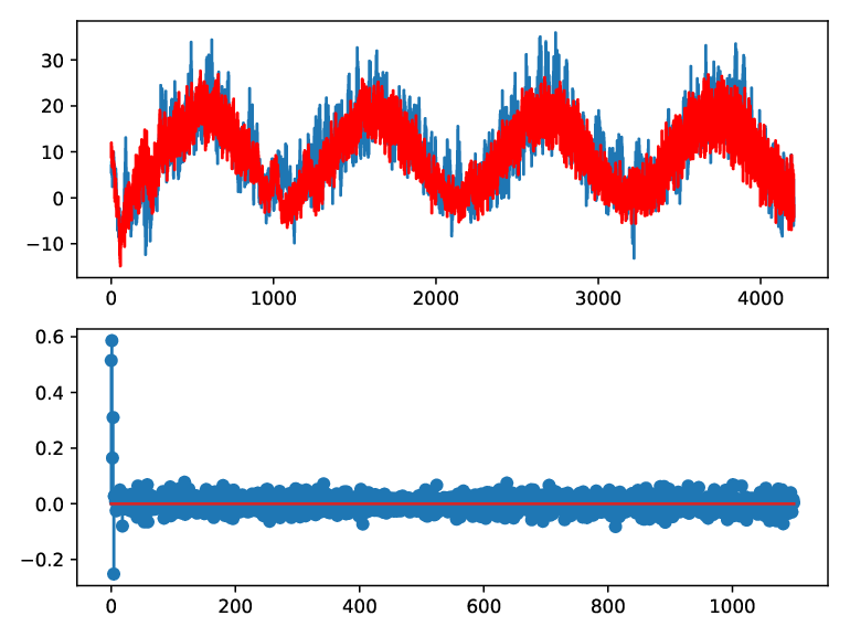
Refer to caption
Figure 14. Reference signal (blue line) and model prediction (red line) (top). Model parameters computed using AutoReg. (bottom).

Since the model computed with AutoReg has 11001100 nonzero coefficients, the recurrence relation corresponding to the model computed with AutoReg will not be written explicitly.

The reference signal, the predicted signal and the model parameters ckc_{k} computed with algorithm 2 using SINDy.m are shown in figure 15.

Refer to caption
Figure 15. Reference signal (black line) and model prediction (red line) (top). Model parameters computed using SINDy.m (bottom).

The reference signal, the predicted signal and the model parameters ckc_{k} computed with algorithm 2 using SpSolver.m are shown in figure 16.

Refer to caption
Figure 16. Reference signal (black line) and model prediction (red line) (top). Model parameters computed using SpSolver.m (bottom).

Although the models computed with SpSolver.m and SINDy.m, both have only 63 nonzero parameters ckc_{k}, we will not write the recurrence relations corresponding to these models explicitly either.

The root mean square error estimates for each model are documented in table 12, and the running times corresponding to the computation of the model parameters are documented in table 13.

Method RMSE
AutoReg 6.2226.222
SINDy 5.89455.8945
SDSI 5.89455.8945
Table 12. Prediction error estimates corresponding to each method.
Method Running Time (seconds)
AutoReg 1.03709697723388671.0370969772338867
SINDy 0.8966530.896653
SDSI 0.5621080.562108
Table 13. Running times for the computation of the local linear model approximant.

The computational setting used for the experiments performed in this section is documented in the Matlab program SpTSPredictor.m and the Python program TSModel.py in [31], these programs can be used to replicate these experiments.

6. Conclusion

The results in §3 and §4 in the form of algorithms like the ones described in §5.1, can be effectively used for the sparse identification of dynamical models that can be used to compute data-driven predictive numerical simulations.

One of the main advantages of the low-rank approximation approach presented in this document, concerns the parameter estimation for linear and nonlinear models where numerical or measurement noises could affect the estimates significantly, an example of this phenomenon is documented as part of the numerical experiment 5.2.1.

7. Future Directions

As a consequence of theorem 4.3, it is possible to approach system identification problems as approximate matrix completion problems via low-rank matrix approximation, the corresponding connections with local low-rank matrix approximation in the sense of [20] will be studied as part of the future directions of this research project.

As observed by Koch in [19], when applying sparse system identification techniques like the ones presented in this document, arriving at a high-quality model will be strongly related with the choice of functions in the method’s library, which may require expert knowledge or tuning, and this consideration aligns perfectly with the philosophy behind the development of the system identification technology presented as part of the results reported in this article.

Computational implementations of the the sparse solvers and identification algorithms presented in this document to the computation of sparse signal models and signal compressions, using rectangular sparse submatrices of wavelet matrices, will also be the subject of future communications.

The connections of the results in §4 to the solution of problems related to controllability and realizability of finite-state systems in classical and quantum information and automata theory in the sense of [4, 2, 30, 5], will be further explored.

Further applications of sparse signal model identification schemes to industrial automation and building information modeling (BMI) technologies, will be further explored.

Data Availability

The programs and data that support the findings of this study are openly available in the SDSI repository, reference number [31].

Conflicts of Interest

The author declares that he has no conflicts of interest.

Acknowledgment

The structure preserving matrix computations needed to implement the algorithms in §5.1, were performed with Matlab R2021a (9.10.0.1602886) 64-bit (glnxa64), Python 3.8.5, Julia 1.6.0 and Netgen/NGSolve 6.2, with the support and computational resources of the Scientific Computing Innovation Center (CICC-UNAH) of the National Autonomous University of Honduras.

I am grateful with Terry Loring, Stan Steinberg, Concepción Ferrufino, Marc Rieffel and Moody Chu for interesting conversations, that have been very helpful for the preparation of this document.

References

  • [1] Rajendra Bhatia. Matrix Analysis, volume 169. Springer, 1997.
  • [2] A. M. Bloch, R. W. Brockett, and C. Rangan. Finite controllability of infinite-dimensional quantum systems. IEEE Transactions on Automatic Control, 55(8):1797–1805, Aug 2010.
  • [3] Christos Boutsidis and Malik Magdon-Ismail. A note on sparse least-squares regression. Information Processing Letters, 114(5):273–276, 2014.
  • [4] R. Brockett and A. Willsky. Finite group homomorphic sequential system. IEEE Transactions on Automatic Control, 17(4):483–490, August 1972.
  • [5] R. W. Brockett. Reduced complexity control systems. IFAC Proceedings Volumes, 41(2):1 – 6, 2008. 17th IFAC World Congress.
  • [6] Steven L. Brunton, Joshua L. Proctor, and J. Nathan Kutz. Discovering governing equations from data by sparse identification of nonlinear dynamical systems. Proceedings of the National Academy of Sciences, 113(15):3932–3937, 2016.
  • [7] Jie Chen, Haim Avron, and Vikas Sindhwani. Hierarchically compositional kernels for scalable nonparametric learning. Journal of Machine Learning Research, 18(66):1–42, 2017.
  • [8] Francois Chollet. Deep Learning with Python. Manning Publications Co., USA, 1st edition, 2017.
  • [9] J. J. Collins and I. N. Stewart. Coupled nonlinear oscillators and the symmetries of animal gaits. Journal of Nonlinear Science, 3(1), 1993.
  • [10] J. J. Collins and I. N. Stewart. A group-theoretic approach to rings of coupled biological oscillators. Biological Cybernetics, 71(2), 1994.
  • [11] M. Farhood and G. E. Dullerud. Lmi tools for eventually periodic systems. Systems & Control Letters, 47(5):417 – 432, 2002.
  • [12] Marc Finzi, S. Stanton, Pavel Izmailov, and A. Wilson. Generalizing convolutional neural networks for equivariance to lie groups on arbitrary continuous data. In ICML, 2020.
  • [13] John E. Franke and James F. Selgrade. Attractors for discrete periodic dynamical systems. Journal of Mathematical Analysis and Applications, 286(1):64–79, 2003.
  • [14] Michael H. Freedman and William H. Press. Truncation of wavelet matrices: Edge effects and the reduction of topological control. Linear Algebra and its Applications, 234:1–19, 1996.
  • [15] Gene H. Golub and Charles F. Van Loan. Matrix Computations. The Johns Hopkins University Press, Baltimore, 4th edition, 2013.
  • [16] R. A. Horn. Topics in Matrix Analysis. Cambridge University Press, USA, 1986.
  • [17] Kadierdan Kaheman, J. Nathan Kutz, and Steven L. Brunton. Sindy-pi: a robust algorithm for parallel implicit sparse identification of nonlinear dynamics. Proceedings of the Royal Society A: Mathematical, Physical and Engineering Sciences, 476(2242):20200279, 2020.
  • [18] E. Kaiser, J. N. Kutz, and S. L. Brunton. Sparse identification of nonlinear dynamics for model predictive control in the low-data limit. Proceedings of the Royal Society A: Mathematical, Physical and Engineering Sciences, 474(2219):20180335, 2018.
  • [19] J. Koch. Data-driven modeling of nonlinear traveling waves. Chaos: An Interdisciplinary Journal of Nonlinear Science, 31(4):043128, 2021.
  • [20] Joonseok Lee, Seungyeon Kim, Guy Lebanon, Yoram Singer, and Samy Bengio. Llorma: Local low-rank matrix approximation. J. Mach. Learn. Res., 17(1):442–465, January 2016.
  • [21] Terry A. Loring and Fredy Vides. Computing floquet hamiltonians with symmetries. Journal of Mathematical Physics, 61(11):113501, 2020.
  • [22] V. Moskvina and K. M. Schmidt. Approximate projectors in singular spectrum analysis. SIAM Journal on Matrix Analysis and Applications, 24(4):932–942, 2003.
  • [23] J. L. Proctor, S. L. Brunton, and J. N. Kutz. Dynamic mode decomposition with control. SIAM J Appl. Dyn. Syst., 15(1):142–161, 2016.
  • [24] J.I. Ramos and F.R. Villatoro. The nonlinear schrödinger equation in the finite line. Mathematical and Computer Modelling, 20(3):31–59, 1994.
  • [25] Fabio Della Rossa, Louis Pecora, Karen Blaha, Afroza Shirin, Isaac Klickstein, and Francesco Sorrentino. Symmetries and cluster synchronization in multilayer networks. Nature Communications, 11(1), 2020.
  • [26] Anastasiya Salova, Jeffrey Emenheiser, Adam Rupe, James P. Crutchfield, and Raissa M. D’Souza. Koopman operator and its approximations for systems with symmetries. Chaos: An Interdisciplinary Journal of Nonlinear Science, 29(9):093128, 2019.
  • [27] Hayden Schaeffer, Giang Tran, Rachel Ward, and Linan Zhang. Extracting structured dynamical systems using sparse optimization with very few samples. Multiscale Modeling & Simulation, 18(4):1435–1461, 2020.
  • [28] P. J. Schmid. Dynamic mode decomposition of numerical and experimental data. J. Fluid Mech., 656:5–28, 2010.
  • [29] J. Schöberl. Netgen an advancing front 2d/3d-mesh generator based on abstract rules. Computing and Visualization in Science, 1:41–52, 1997.
  • [30] D. C. Tarraf. An input-output construction of finite state ρ/μ\rho/\mu approximations for control design. IEEE Transactions on Automatic Control, 59(12):3164–3177, Dec 2014.
  • [31] F. Vides. SDSI: A toolset with matlab, python and julia programs for approximate sparse system identification, 2021. https://github.com/FredyVides/SDSI.
  • [32] Rok Vrabič, John Ahmet Erkoyuncu, Peter Butala, and Rajkumar Roy. Digital twins: Understanding the added value of integrated models for through-life engineering services. Procedia Manufacturing, 16:139–146, 2018. Proceedings of the 7th International Conference on Through-life Engineering Services.
  • [33] Louise Wright and Stuart Davidson. How to tell the difference between a model and a digital twin. Advanced Modeling and Simulation in Engineering Sciences, 7(1), 2020.