Graph-Free Knowledge Distillation for Graph Neural Networks Code: https://github.com/Xiang-Deng-DL/GFKD
Abstract
Knowledge distillation (KD) transfers knowledge from a teacher network to a student by enforcing the student to mimic the outputs of the pretrained teacher on training data. However, data samples are not always accessible in many cases due to large data sizes, privacy, or confidentiality. Many efforts have been made on addressing this problem for convolutional neural networks (CNNs) whose inputs lie in a grid domain within a continuous space such as images and videos, but largely overlook graph neural networks (GNNs) that handle non-grid data with different topology structures within a discrete space. The inherent differences between their inputs make these CNN-based approaches not applicable to GNNs. In this paper, we propose to our best knowledge the first dedicated approach to distilling knowledge from a GNN without graph data. The proposed graph-free KD (GFKD) learns graph topology structures for knowledge transfer by modeling them with multivariate Bernoulli distribution. We then introduce a gradient estimator to optimize this framework. Essentially, the gradients w.r.t. graph structures are obtained by only using GNN forward-propagation without back-propagation, which means that GFKD is compatible with modern GNN libraries such as DGL and Geometric. Moreover, we provide the strategies for handling different types of prior knowledge in the graph data or the GNNs. Extensive experiments demonstrate that GFKD achieves the state-of-the-art performance for distilling knowledge from GNNs without training data.
1 Introduction
Knowledge Distillation (KD) Hinton et al. 2015 aims to transfer useful knowledge from a teacher network to a student. The effectiveness of KD to boost the student performance has been demonstrated across a wide range of applications in artificial intelligence Romero et al. 2015. As the knowledge in a teacher concentrates on a narrow manifold instead of the full input space, KD has a strong assumption that either the training dataset or some representative samples are available. The requirement for observable data highly limits its applications on data-unavailable cases. For example, a deep model (e.g., ResNet-152) that is pretrained on a large-scale dataset of billions of data samples is released online. One may wish to distill the knowledge from this powerful model into a compact and fast model for the deployment on resource-limited devices, which requires the access to the training dataset. However, the dataset is not publicly available as it is not only large but also difficult to store and transfer. In reality, it is not rare that a corporation or a leading research group shares their pretrained models while they do not release the training data due to large sizes, privacy, confidentiality, or security in medical or industrial domains.

A simple yet effective way to address the issue is to generate fake data for knowledge transfer by optimizing the inputs to the pretrained teacher to maximize the class-conditional probability Mordvintsev et al.. This method Yin et al. 2020 has shown its success on convolutional neural networks (CNNs) where the inputs are grid data within a continuous space such as images and videos as the gradients w.r.t. the inputs exist. However, many real data such as proteins and chemical molecules lie in non-grid domains within a discrete space and thus call for graph neural networks (GNNs) Kipf and Welling 2017 that explicitly deal with the topological structures of these graph data. As shown in Figure 1, different from CNNs handling grid data such as images, GNNs deal with graph data that contain both node features and topological structures within a discrete space. Current GNN models learn the node-level or graph-level representations by aggregating node features based on local topology structures. The output of a GNN is not differentiable w.r.t. the topological structures of the input graphs, which makes the CNN-based approaches not applicable to GNNs.
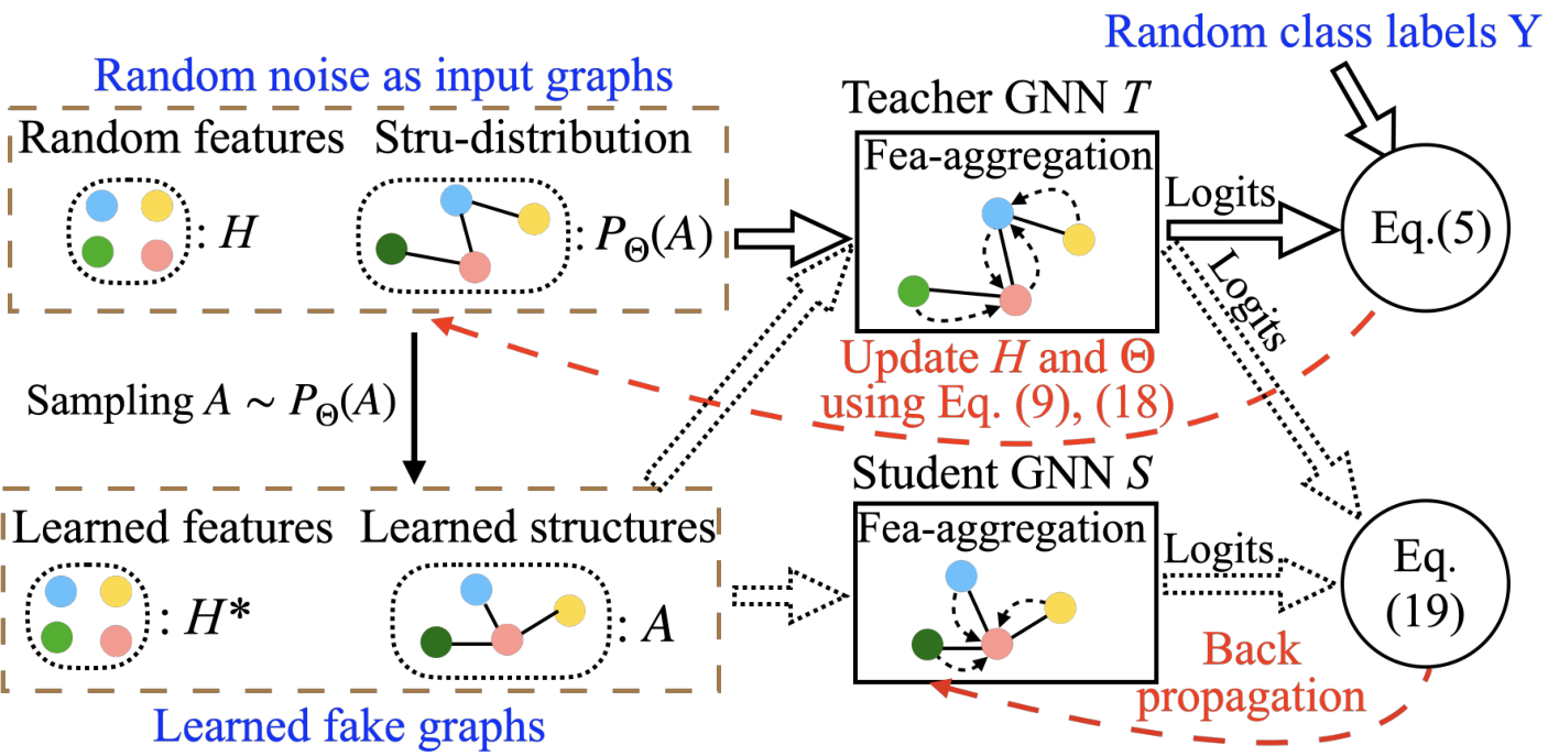
In this paper, we study how to distill knowledge from a pretrained GNN without observable graphs and develop to the best of our knowledge the first data-free knowledge distillation approach (i.e., GFKD) tailored for GNNs. The workflow of GFKD is shown in Figure 2. GFKD first learns the fake graphs that the knowledge in the teacher GNN is more likely to concentrate on, and then uses these fake graphs to transfer knowledge to the student. To achieve this goal, we propose a structure learning strategy by modeling the topology of a graph with a multivariate Bernoulli distribution and then introduce a gradient estimator to optimize it.
Our main contributions are summarized as follows:
- •
We introduce a novel framework, i.e., GFKD, for distilling knowledge from GNNs without observable graph data. To the best of our knowledge, this is the first dedicated data-free KD approach tailored for GNNs. We also provide the strategies (or regularizers) for handling different priors about the graph data, including how to deal with one-hot features and degree features.
- •
We develop a novel strategy for learning graph structures from a pretrained GNN by using multivariate Bernoulli distribution and introduce a gradient estimator to optimize it, which paves the way for extracting knowledge from a pretrained GNN without observable graphs. Note that the current GNN libraries do not support computing gradients w.r.t. the input graph structures. GFKD avoids this issue as the structure gradients in GFKD are obtained by only using GNN forward propagation without backward propagation. GFKD is thus supported by these libraries.
- •
We evaluate GFKD on six benchmark datasets in different domains with two different GNN architectures under different settings and demonstrate that GFKD achieves the best performance across different datasets.
2 Related Work
2.1 Graph Neural Networks
GNNs emerge as a hot topic in recent years for their potential in numerous applications. Bruna et al. Bruna et al. 2013 first generalize CNNs to signals defined on the non-grid domain. Defferrard et al. Defferrard et al. 2016 further improve the idea by using Chebyshev polynomials. Kipf and Welling Kipf and Welling 2017 propose to build GNNs by stacking multiple first-order Chebyshev polynomial filters. Xu et al. Xu et al. 2019, on the other hand, propose a simple neural architecture, graph isomorphism networks (GINs), which generalizes the Weisfeiler-Lehman (WL) test and hence achieves a powerful discriminative ability. The other GNN architectures including but not limited to Fey et al. 2018; Li et al. 2015; Hamilton et al. 2017; Veličković et al. 2017 deal with the features and the topological structures using different strategies.
2.2 Knowledge Distillation
Knowledge distillation aims at transferring knowledge from a teacher model to a student. Hinton et al. Hinton et al. 2015 propose KD that penalizes the softened logit differences between a teacher and a student. FitNet Romero et al. 2015 and AT Zagoruyko and Komodakis 2017 further use the feature alignment to assist knowledge transfer. Yang et al. Yang et al. 2020 develop a local structure preserving module for distilling knowledge from GNNs. Other distillation approaches Tian et al. 2020 use different criteria to align feature representations. All these approaches require the training dataset for knowledge transfer, which cannot handle the case where the training data are not available.
To address this issue, many efforts have been made on distilling knowledge without training images from a CNN through generating fake images. Lopes et al. Lopes et al. 2017 make use of meta data instead of real images to distill knowledge. Yoo et al. Yoo et al. 2019 use a generator and a decoder to learn fake images for knowledge transfer. Micaelli and Storkey Micaelli and Storkey 2019 and Chen et al Chen et al. 2019 use generative adversarial networks (GANs) Goodfellow et al. 2014 to generate fake images. Nayak et al. Nayak et al. 2019 propose to generate images by modelling the softmax space. DeepInversion Yin et al. 2020 generates fake images by inversing a CNN and using the statistics in batch normalization Ioffe and Szegedy 2015.
All these data-free KD approaches are designed for CNNs with images as inputs, and highly overlook GNNs dealing with non-grid data within a discrete space. Directly applying these approaches to GNNs is not applicable as graph data contain both features and topological structures. Thus, it is necessary and appealing to develop a data-free KD approach tailored for GNNs.
3 Framework
In this section, we first provide a brief overview on GNNs. We then present GFKD and the strategies for dealing with different types of prior knowledge about the graph data. At the end, we introduce the optimization solution to GFKD.
3.1 Graph Neural Networks
Different from CNNs handling grid data, GNNs can take non-gird data as inputs. A non-grid data can be represented as a graph and a set of features , where and denote the nodes and the edges, respectively. Modern GNNs typically adopt a neighborhood aggregation strategy by using the features and graph structures to learn discriminative node or graph representations. Suppose that is the feature of node . The operation in layer of a GNN is:
| (1) |
where denotes the aggregation function; is the feature transformation function; denotes the neighbors of node . It is observed that the topological structure of a graph plays a vital role in learning representations. To transfer the knowledge from a teacher GNN to a student, it is necessary to know which structures the knowledge concentrates on.
3.2 Graph-Free Knowledge Distillation
Suppose that a teacher GNN with parameters is trained over dataset (X, Y) by minimizing the regular cross-entropy loss, where X and Y are the graph data and the labels, respectively:
| (2) |
where denotes the loss function such as cross-entropy or mean square error; denotes the node features of graphs X; represents the graph structure information of X which can be represented as adjacency matrices consisting of 0s and 1s.
From the Bayesian perspective, learning by minimizing (2) can be considered as maximizing the logarithm of class-conditional probability , i.e., = . Thus, the knowledge is more likely to concentrate on the graphs that make the teacher output a high class-conditional probability. When training data are not available but is known, one may optimize the inputs by maximizing the class-conditional probability (i.e., or ) to generate fake samples for knowledge transfer. This inversion technique Yin et al. 2020 has shown its success on CNNs where the inputs are grid-data images within a continuous space without topological structures . Unfortunately, this is not applicable to GNNs as is not differentiable w.r.t. the graph structure (but differentiable w.r.t. features ) as seen from (1).
3.2.1 Learning Graph Topology with Stochastic Structures
To address the above issue, we propose to model the topological structure of a graph with a multivariate Bernoulli distribution, thus obtaining a stochastic structure. Specifically, suppose that is the structure (i.e., adjacency matrix) of a graph. Each element in follows a Bernoulli distribution:
| (3) |
where is the sigmoid function ; is a learnable parameter; is the element in the th row and the th column in where means that node is a neighbor of and vice versa.
For directed graphs, parameters are used to model the distribution of :
| (4) |
Note that for undirected graphs, the number of parameters is reduced to as their adjacency matrices are symmetric.
For a batch of graphs, their structures are independent of each other and thus follow the joint distribution: where is the number of graphs and is the structure parameter for graph . Instead of directly minimizing (2) that is not differentiable w.r.t. , we generate fake graph data by minimizing the following expectation11 1 Assume that we have some priors about the magnitude of the number of graph data nodes.:
| (5) |
where = ; represents the feature parameters; is a set of randomly sampled labels; denotes the regularizers for different priors that we have about the target task data; is a balancing weight. Thus, minimizing (5) w.r.t. and can generate the graph data that maximize the GNN output class probability. We omit in in the following as it is known for a pretrained teacher GNN.
3.2.2 Regularizers for Prior Knowledge
in (5) deals with different types of prior knowledge about the graph data for the target task. We provide the strategies for handling common priors.
Priors in Graph Neural Networks:
Similar to the case in CNNs, many GNNs also benefit from batch normalization (BN). BN contains statistical information about the data as it accumulates the moving average of the means and the variances of the features during training. Similar to the case in CNNs Yin et al. 2020, it is reasonable to force the fake graph data to have similar feature means and variances to those in the GNNs accumulated from the real graph data:
| (6) |
where and represent the means and variances of the features of the generated graphs, respectively; and are the means and variances in the teacher GNN, respectively.
Priors about Target-Task Graph Data:
Besides the priors embedded in the GNNs, one may have some prior knowledge about the target task data:
(1) One-hot features:
The graph data for many tasks have one-hot features, such as the classification task on MUTAG. In this case, directly minimizing (5) cannot lead to one-hot features. To address this issue, we first reparameterize in (5) with the softmax function where are learnable parameters and then minimize the entropy of :
| (7) |
where denotes the entropy and can be seen as the instantiations of .
(2) Degrees as features:
Some graph data use the degrees of the nodes as features. In this case, the features can be derived from the adjacency matrix . It is thus not necessary to explicitly learn features and objective (5) is reduced to:
| (8) |
We have discussed some common graph priors while there may be other priors for different graphs. Fortunately, objective (5) is readily extended to different graph data.
3.2.3 Optimization
To minimize objective (5), we need to compute the gradients regarding and . As the gradients of w.r.t. exist, we can easily estimate them by sampling from :
| (9) |
where are independent and identically distributed (iid).
The difficulty lies in computing the gradients w.r.t. that exist in the distribution . We introduce a gradient estimator Yin and Zhou 2019; Williams 1992 to optimize , which is based on the reparametrization trick and REINFORCE.
We omit in the objective (5) in the following for simplicity. Bernoulli random variables in (5) can be reparameterized by two exponential random variables:
| (10) |
where represents the Exponential distribution; denotes the element-wise product; is the indicator function which equals to one if the argument is true and zero otherwise.
Note that as follows , = follows . Similarly, = follows . (10) can be further reparameterized as:
| (11) |
Next we show how to obtain the gradients w.r.t . Applying REINFORCE to (11) leads to:
| (12) |
As = and = , (12) is equivalent to:
| (13) |
and can be further reparameterized as:
| (14) |
where and follow and , respectively, and and denote the uniform distribution and the gamma distribution, respectively. (13) can be further reparameterized as:
| (15) |
By applying Rao Blackwellization to (15), is equal to:
| (16) |
implies . Thus, in (16) can be replaced with to obtain a new unbiased gradient estimator. Taking the average of the new estimator and (16) can further reduce the sampling variance Yin and Zhou 2019:
| (17) |
By simply sampling from , we can obtain the gradients w.r.t.
| (18) |
where are iid. More derivation details are given in the Appendix. We set to 1 in this paper as the variance is small. As shown in (18), this unbiased gradient estimator allows us to obtain the gradients w.r.t. the structure parameters with only GNN forward propagation and thus it is efficient and supported by the current GNN libraries.
| Datasets | MUTAG | PTC | PROTEINS | |||||||
| Teacher | GCN-5-64 | GIN-5-64 | GCN-5-64 | GCN-5-64 | GIN-5-64 | GCN-5-64 | GCN-5-64 | GIN-5-64 | GCN-5-64 | |
| Student | GCN-3-32 | GIN-3-32 | GIN-3-32 | GCN-3-32 | GIN-3-32 | GIN-3-32 | GCN-3-32 | GIN-3-32 | GIN-3-32 | |
| Teacher | 100% training data | 89.5 | 92.9 | 89.5 | 63.5 | 61.5 | 63.5 | 76.9 | 76.0 | 76.9 |
| KD | 100% training data | 84.62.3 | 87.72.1 | 84.41.7 | 60.22.1 | 60.51.9 | 60.62.6 | 76.01.0 | 76.70.6 | 76.30.8 |
| RandG | 0 training data | 39.16.8 | 58.74.2 | 38.85.8 | 43.24.4 | 53.25.8 | 42.98.0 | 56.64.8 | 33.37.4 | 43.49.5 |
| DeepInvG | 0 training data | 58.65.1 | 59.62.9 | 35.42.2 | 52.97.8 | 45.74.1 | 43.99.2 | 65.42.3 | 52.75.7 | 47.49.9 |
| GFKD | 0 training data | 70.82.1 | 73.24.2 | 70.22.0 | 57.42.2 | 57.52.4 | 54.16.4 | 74.71.5 | 60.41.0 | 65.53.1 |
| Datasets | IMDB-B | COLLAB | REDDIT-B | |||||||
|---|---|---|---|---|---|---|---|---|---|---|
| Teacher | GCN-5-64 | GIN-5-64 | GCN-5-64 | GCN-5-64 | GIN-5-64 | GCN-5-64 | GCN-5-64 | GIN-5-64 | GCN-5-64 | |
| Student | GCN-3-32 | GIN-3-32 | GIN-3-32 | GCN-3-32 | GIN-3-32 | GIN-3-32 | GCN-3-32 | GIN-3-32 | GIN-3-32 | |
| Teacher | 100% training data | 74.3 | 75.3 | 74.3 | 81.7 | 82.3 | 81.7 | 92.8 | 91.7 | 92.8 |
| KD | 100% training data | 76.40.8 | 75.40.9 | 75.61.3 | 80.90.6 | 81.90.5 | 81.60.4 | 85.70.6 | 88.42.5 | 87.23.4 |
| RandG/DeepInvG | 0 training data | 58.53.7 | 58.74.2 | 55.43.4 | 34.89.0 | 28.47.3 | 27.26.3 | 50.11.0 | 49.90.8 | 48.92.1 |
| GFKD | 0 training data | 69.21.1 | 67.81.8 | 67.12.3 | 67.31.4 | 65.42.7 | 66.81.8 | 66.53.7 | 63.84.5 | 63.15.7 |
| #Graphs | #Classes | Avg#Graph Size | |
|---|---|---|---|
| MUTAG | 188 | 2 | 17.93 |
| PTC | 344 | 2 | 14.29 |
| PROTEINS | 1,113 | 2 | 39.06 |
| IMDB-B | 1,000 | 2 | 19.77 |
| COLLAB | 5,000 | 3 | 74.49 |
| REDDIT-B | 2,000 | 2 | 429.62 |
3.2.4 Knowledge Transfer with Generated Fake Graphs
As shown in Figure 2, we first update feature parameters and the stochastic structure parameters by minimizing (5) with gradients (9) and (18), respectively. We then simply obtain fake graphs by using as the node features and sampling from to generate topological structures. The teacher GNN outputs a high probability on these graphs and thus the knowledge is more likely to concentrate on these graphs. We then transfer knowledge from the teacher to the student by using these fake graph data with the KL-divergence loss:
| (19) |
where is the softmax function; is a temperature to generate soft labels and represents KL-divergence; is the student GNN. To the end, we achieve knowledge distillation without any observable graphs.
4 Experiments
In this section, we report extensive experiments for evaluating GFKD. Note that our goal is not to generate real graphs but to transfer as much knowledge as possible from a pretrained teacher GNN to a student without using any training data.
4.1 Experimental Settings
We adopt six graph classification benchmark datasets Xu et al. 2019 including three bioinformatics graph datasets, i.e., MUTAG, PTC, and PROTEINS, and three social network graph datasets, i.e., IMDB-B, COLLAB, and REDDIT-B. The statistics of these datasets are summarized in Table 3. On each dataset, 70% data are used for pretraining the teachers and the remaining 30% are used as the test data.
We use two well known GNN architectures, i.e, GCN Kipf and Welling 2017 and GIN Xu et al. 2019. We distill knowledge in two different settings, i..e, the teacher and the student share the same architecture or use different architectures. We use the form of (architecture-layer number-feature dimensions) to denote a GNN. For example, GIN-5-64 denotes a GNN with 5 GIN layers and 64 feature dimensions.
As there is no existing approach applicable to GNNs for distilling knowledge without observable graph data, we design two baselines for references:
- •
Random Graphs (RandG): RandG generates fake graphs by randomly drawing from a uniform distribution as node features and topological structures, and then use these graphs to transfer knowledge.
- •
DeepInvG Yin et al. 2020: As the original DeepInversion Yin et al. 2020 cannot learn the structures of graph data, here DeepInvG first randomly generates graph structures and then uses DeepInversion to learn node features with objective .
For generating fake graphs, we do 2500 iterations. The learning rates for structure and feature parameters are set to 1.0 (5.0 on PROTEINS, COLLAB, and REDDIT-B) and 0.01, respectively, and are divided by 10 every 1000 iterations. For KD, all the GNNs are trained for 400 epochs with Adam and the learning rate is linearly decreased from 1.0 to 0. is set to 2. More details are given in the Appendix.


4.2 Experiments on Bioinformatics Graph Data
Table 1 reports the comparison results on three bioinformatics graph datasets. It is observed that without using any training data, GFKD transfers much more knowledge than those of the baselines across different datasets and architectures, which demonstrates the effectiveness of GFKD. As expected, the overall performance of RandG is worse than those of the other methods as the knowledge in the teacher does not concentrate on random graphs. GFKD and DeepInvG both learn node features for fake graphs, but differ in that GFKD learns graph structures while DeepInvG randomly generates structures. As shown in Table 1, GFKD improves the accuracy over DeepInvG substantially. For example, the accuracy improvement of GFKD is 12.2% over DeepInvG with teacher GCN-5-64 and student GCN-3-32 on MUTAG. This demonstrates the effectiveness of GFKD for learning graph structures. We also notice that in the teacher-student pair with different architectures, i.e, GCN-5-64 and GIN-3-32, GFKD also beats the baselines significantly on all the three datasets, which demonstrates that GFKD is applicable to the case where the teacher and the student have different architectures.
4.3 Experiments on Social Network Graph Data
To investigate the generalization of GFKD in different domains, we further conduct experiments on three social network graph datasets. Table 2 reports the comparison results. Note that on the three datasets, the node features are the degrees of the nodes (or a constant) which are derived from the graph structures. Thus, DeepInvG is reduced to RandG. It is observed that GFKD also outperforms the baselines substantially on all the three social network datasets, which demonstrates the generalization and usefulness of GFKD for different types of graph data. The superiority of GFKD is attributed to its ability to learn the topology structures of graph data.
4.4 Ablation Studies
4.4.1 Ablation Studies regarding the Number of Fake Graphs
Theoretically, GFKD can generate infinite fake graphs for knowledge transfer. However, the quality and the diversity are limited by the pretrained teacher. We study how the performance of GFKD varies with the number of fake samples. We denote the ratio of the number of fake graphs to the number of training samples used by the teacher by .
Figure 6 presents the effects of the number of fake graphs, where GCN-5-64 and GCN-3-32 are adopted as the teacher and the student, respectively. It is not surprising that the performances of GFKD first increase and then stabilize. The reason for the performance stabilization is that the diversity of the generated graphs is constrained by the pretrained teacher.
4.4.2 Ablation Studies regarding the Regularizers
We have introduced two regularizers dealing with BN and one-hot features, respectively. We evaluate their effects on the performances of GFKD by using GCN-5-64 and GCN-3-32 as the teacher and the student, respectively. We adopt MUTAG and PTC datasets as their features are one-hot.
The comparison results are presented in Figure 4, where , , and denote GFKD without the BN regularizer, without the one-hot regularizer, and without neither of the two regularizers, respectively. We observe that the performance decreases significantly without either of these two regularizers, which demonstrates the effectiveness and usefulness of these two regularizers. Meanwhile, this also indicates that more prior knowledge about the graph data leads to better performances.
4.5 Visualization
Although the goal of GFKD is not to generate real graph data, we present some fake graphs learned by GFKD in Figure 4, where the fake graphs are learned on IMDB-B from pretrained teacher GCN-5-64. It is observed that the fake graphs and the real graphs share some visual similarities.
To further investigate whether GFKD can learn discriminative features from these fake graphs, we use t-SNE Maaten and Hinton 2008 to visualize the features learned by different methods. We adopt GCN-5-64 and GCN-3-32 as the teacher and the student in this experiment, respectively.
Figure 6 presents the visualization of the features learned by RandG, GFKD, and the teacher. It is observed that the feature representations learned by RandG are mixed for different classes, which indicates that using randomly generated graphs cannot learn discriminative features. In contrast, the features learned by GFKD are well separated for different classes and are as discriminative as those learned by the teacher. This demonstrates that the fake samples learned by GFKD are beneficial to representation learning and the knowledge concentrates on these fake graphs.
5 Conclusion
In this paper, we study a novel problem on how to distill knowledge from a GNN without observable graph data and introduce GFKD as a solution, which is to our best knowledge the first work along this line. To learn where the knowledge in the teacher concentrates on, we propose to model the graph structures with multivariate Bernoulli distribution and then introduce a gradient estimator to optimize it. Essentially, the structure gradients can be obtained by only using GNN forward propagation. Extensive experiments on six benchmark datasets demonstrate the superiority of GFKD for extracting knowledge from GNNs without observable graphs.
References
- Bruna et al. [2013] Joan Bruna, Wojciech Zaremba, Arthur Szlam, and Yann LeCun. Spectral networks and locally connected networks on graphs. arXiv preprint arXiv:1312.6203, 2013.
- Chen et al. [2019] Hanting Chen, Yunhe Wang, Chang Xu, Zhaohui Yang, Chuanjian Liu, Boxin Shi, Chunjing Xu, Chao Xu, and Qi Tian. Data-free learning of student networks. In Proceedings of the IEEE International Conference on Computer Vision, pages 3514–3522, 2019.
- Defferrard et al. [2016] Michaël Defferrard, Xavier Bresson, and Pierre Vandergheynst. Convolutional neural networks on graphs with fast localized spectral filtering. In Advances in neural information processing systems, pages 3844–3852, 2016.
- Fey et al. [2018] Matthias Fey, Jan Eric Lenssen, Frank Weichert, and Heinrich Müller. Splinecnn: Fast geometric deep learning with continuous b-spline kernels. In Proceedings of the IEEE Conference on Computer Vision and Pattern Recognition, pages 869–877, 2018.
- Goodfellow et al. [2014] Ian Goodfellow, Jean Pouget-Abadie, Mehdi Mirza, Bing Xu, David Warde-Farley, Sherjil Ozair, Aaron Courville, and Yoshua Bengio. Generative adversarial nets. In Advances in neural information processing systems, pages 2672–2680, 2014.
- Hamilton et al. [2017] Will Hamilton, Zhitao Ying, and Jure Leskovec. Inductive representation learning on large graphs. In Advances in neural information processing systems, pages 1024–1034, 2017.
- Hinton et al. [2015] Geoffrey Hinton, Oriol Vinyals, and Jeff Dean. Distilling the knowledge in a neural network. arXiv preprint arXiv:1503.02531, 2015.
- Ioffe and Szegedy [2015] Sergey Ioffe and Christian Szegedy. Batch normalization: Accelerating deep network training by reducing internal covariate shift. arXiv preprint arXiv:1502.03167, 2015.
- Kipf and Welling [2017] Thomas N Kipf and Max Welling. Semi-supervised classification with graph convolutional networks. International Conference on Learning Representations, 2017.
- Li et al. [2015] Yujia Li, Daniel Tarlow, Marc Brockschmidt, and Richard Zemel. Gated graph sequence neural networks. arXiv preprint arXiv:1511.05493, 2015.
- Lopes et al. [2017] Raphael Gontijo Lopes, Stefano Fenu, and Thad Starner. Data-free knowledge distillation for deep neural networks. arXiv preprint arXiv:1710.07535, 2017.
- Maaten and Hinton [2008] Laurens van der Maaten and Geoffrey Hinton. Visualizing data using t-sne. Journal of machine learning research, 9(Nov):2579–2605, 2008.
- Micaelli and Storkey [2019] Paul Micaelli and Amos J Storkey. Zero-shot knowledge transfer via adversarial belief matching. In Advances in Neural Information Processing Systems, pages 9551–9561, 2019.
- [14] Alexander Mordvintsev, Christopher Olah, and Mike Tyka. Inceptionism: Going deeper into neural networks. https://ai.googleblog.com/2015/06/ inceptionism-going-deeper-into-neural.html, last accessed on 12.20.2020.
- Nayak et al. [2019] Gaurav Kumar Nayak, Konda Reddy Mopuri, Vaisakh Shaj, R Venkatesh Babu, and Anirban Chakraborty. Zero-shot knowledge distillation in deep networks. arXiv preprint arXiv:1905.08114, 2019.
- Romero et al. [2015] Adriana Romero, Nicolas Ballas, Samira Ebrahimi Kahou, Antoine Chassang, Carlo Gatta, and Yoshua Bengio. Fitnets: Hints for thin deep nets. In International Conference on Learning Representations, 2015.
- Tian et al. [2020] Yonglong Tian, Dilip Krishnan, and Phillip Isola. Contrastive representation distillation. In International Conference on Learning Representations, 2020.
- Veličković et al. [2017] Petar Veličković, Guillem Cucurull, Arantxa Casanova, Adriana Romero, Pietro Lio, and Yoshua Bengio. Graph attention networks. arXiv preprint arXiv:1710.10903, 2017.
- Williams [1992] Ronald J Williams. Simple statistical gradient-following algorithms for connectionist reinforcement learning. Machine learning, 8(3-4):229–256, 1992.
- Xu et al. [2019] Keyulu Xu, Weihua Hu, Jure Leskovec, and Stefanie Jegelka. How powerful are graph neural networks? International Conference on Learning Representations, 2019.
- Yang et al. [2020] Yiding Yang, Jiayan Qiu, Mingli Song, Dacheng Tao, and Xinchao Wang. Distilling knowledge from graph convolutional networks. In Proceedings of the IEEE/CVF Conference on Computer Vision and Pattern Recognition, pages 7074–7083, 2020.
- Yin and Zhou [2019] Mingzhang Yin and Mingyuan Zhou. Arm: Augment-reinforce-merge gradient for stochastic binary networks. In International Conference on Learning Representations, 2019.
- Yin et al. [2020] Hongxu Yin, Pavlo Molchanov, Jose M Alvarez, Zhizhong Li, Arun Mallya, Derek Hoiem, Niraj K Jha, and Jan Kautz. Dreaming to distill: Data-free knowledge transfer via deepinversion. In Proceedings of the IEEE/CVF Conference on Computer Vision and Pattern Recognition, pages 8715–8724, 2020.
- Yoo et al. [2019] Jaemin Yoo, Minyong Cho, Taebum Kim, and U Kang. Knowledge extraction with no observable data. In Advances in Neural Information Processing Systems, pages 2705–2714, 2019.
- Zagoruyko and Komodakis [2017] Sergey Zagoruyko and Nikos Komodakis. Paying more attention to attention: Improving the performance of convolutional neural networks via attention transfer. In International Conference on Learning Representations, 2017.