跳到论文正文
W Papers独立论文阅读器 arXiv:2105.07398 论文正文 计算阅读时间 · 0%
引用这篇论文根据当前论文元数据生成,正式投稿前建议核对。


License: CC BY 4.0
arXiv:2105.07398v1 [cs.IT] 16 May 2021

On the Secrecy Rate of Downlink NOMA in Underlay Spectrum Sharing with Imperfect CSI

Vaibhav Kumar1, Mark F. Flanagan1, Daniel Benevides da Costa2, and Le-Nam Tran1 Affiliation: 1School of Electrical and Electronic Engineering, University College Dublin, Belfield, Dublin 4, Ireland
2Future Technology Research Center, National Yunlin University of Science and Technology, Douliu, Yunlin 64002, Taiwan
Email: {vaibhav.kumar, mark.flanagan, danielbcosta}@ieee.org, nam.tran@ucd.ie
Abstract

In this paper, we present the ergodic sum secrecy rate (ESSR) analysis of an underlay spectrum sharing non-orthogonal multiple access (NOMA) system. We consider the scenario where the power transmitted by the secondary transmitter (ST) is constrained by the peak tolerable interference at multiple primary receivers (PRs) as well as the maximum transmit power of the ST. The effect of channel estimation error is also taken into account in our analysis. We derive exact and asymptotic closed-form expressions for the ESSR of the downlink NOMA system, and show that the performance can be classified into two distinct regimes, i.e., it is dictated either by the interference constraint or by the power constraint. Our results confirm the superiority of the NOMA-based system over its orthogonal multiple access (OMA) based counterpart. More interestingly, our results show that NOMA helps in maintaining the secrecy rate of the strong user while significantly enhancing the secrecy performance of the weak user as compared to OMA. The correctness of the proposed investigation is corroborated through Monte Carlo simulation.

††papernotice: Invited Paper††footnotetext: This publication has emanated from research conducted with the financial support of Science Foundation Ireland (SFI) and is co-funded under the European Regional Development Fund under Grant Number 17/CDA/4786.

I Introduction

Non-orthogonal multiple access (NOMA) has gained tremendous attention as a potential multiple access technology for the next-generation wireless systems. It is proven to be capable of providing massive connectivity, low latency and higher achievable rate as compared to the traditional orthogonal multiple access (OMA) system [1]. In order to serve multiple users using a given resource block (time slot, frequency band, and/or spreading code), NOMA uses power-division multiplexing at the transmitter’s side and successive interference cancellation (SIC) at the receivers’ side. Underlay spectrum sharing is another potential technology to mitigate the problem of spectrum scarcity, where an unlicensed/secondary network simultaneously uses the spectrum owned by a licensed/primary network in such a manner that the interference inflicted by the secondary network on the primary one remains below a certain threshold [2]. The benefits of underlay spectrum sharing NOMA systems over their OMA-based counterparts were discussed in [3, 4, 5].

In today’s privacy-concerned society, the broadcast nature of radio waves poses a significant risk that wireless communications may be intercepted by an eavesdropper. Therefore, physical-layer security (PLS), which provides an additional layer of security from an information-theoretic perspective, has gained significant attention in the past couple of decades [6]. The secrecy outage probability (SOP) analysis of a multiple-relay-assisted two-user downlink NOMA system was presented in [7], where the authors proposed different relay selection schemes to enhance the secrecy performance of the system. The ergodic sum secrecy rate (ESSR) analysis of a two-user downlink and uplink cooperative NOMA system with untrusted relaying was performed in [8], while the authors in [9] presented the ergodic secrecy rate (ESR) and SOP analysis of a full-duplex relay-assisted two-user downlink NOMA system with energy harvesting.

On the other hand, some recent contributions on the secrecy analysis of underlay spectrum sharing systems include [10, 11, 12]. Specifically, the secrecy throughput and energy efficiency analysis of a spectrum sharing system consisting of one primary source-destination pair, multiple secondary source-destination pairs and an eavesdropper was presented in [10], where primary and secondary networks either interfere or cooperate with each other in order to improve the secrecy performance. In [11], the authors derived closed-form expressions for the non-zero secrecy rate, ESR and SOP of an outage-constrained spectrum sharing system with transmitter selection and unreliable backhaul. The analysis of the achievable secrecy rate for an underlay spectrum sharing multi-user massive multiple-input multiple-output (mMIMO) system was presented in [12]. However, to the best of the authors’ knowledge, the secrecy rate analysis of an underlay spectrum sharing system where the secondary transmitter communicates with the secondary receivers using NOMA has not yet been investigated in the literature. Therefore, in this paper, we present the ESSR analysis of a two-user downlink NOMA system in an underlay spectrum sharing scenario. The main contributions in this paper are listed below:

  • •

    We derive an exact closed-form expression for the ESSR of a downlink NOMA system in an underlay spectrum sharing scenario with multiple primary receivers (PRs) considering the effect of imperfect channel state information (CSI). We show the effect of the peak tolerable interference power at the PRs, the maximum power budget at the secondary transmitter (ST), channel estimation error and the number of PRs on the ESSR of the NOMA system.

  • •

    We derive an asymptotic expression for the ESSR of the downlink NOMA system for large values of peak tolerable interference at the PRs. The asymptotic analysis confirms that the slope of the ESSR tends to zero (w.r.t. the peak tolerable interference at the PRs), and the ESSR becomes independent of the number of PRs as well as the quality of the channel between the ST and PRs.

  • •

    Using the exact closed-form expressions for the ESR, we perform a one-dimensional numerical search to allocate power between the NOMA users in such a manner that the ESR of the strong user in the NOMA system and the corresponding OMA system becomes equal, and then the remaining power is allocated to the weak NOMA user. Such a power allocation policy ensures that the secrecy performance of the strong user in the NOMA system is the same as that of the strong user in the corresponding OMA system while the secrecy performance of the weak user in the NOMA system is enhanced significantly as compared to that in the OMA system, resulting in a performance superiority of the NOMA system over its OMA-based counterpart in terms of ESSR.

II System Model
Refer to caption
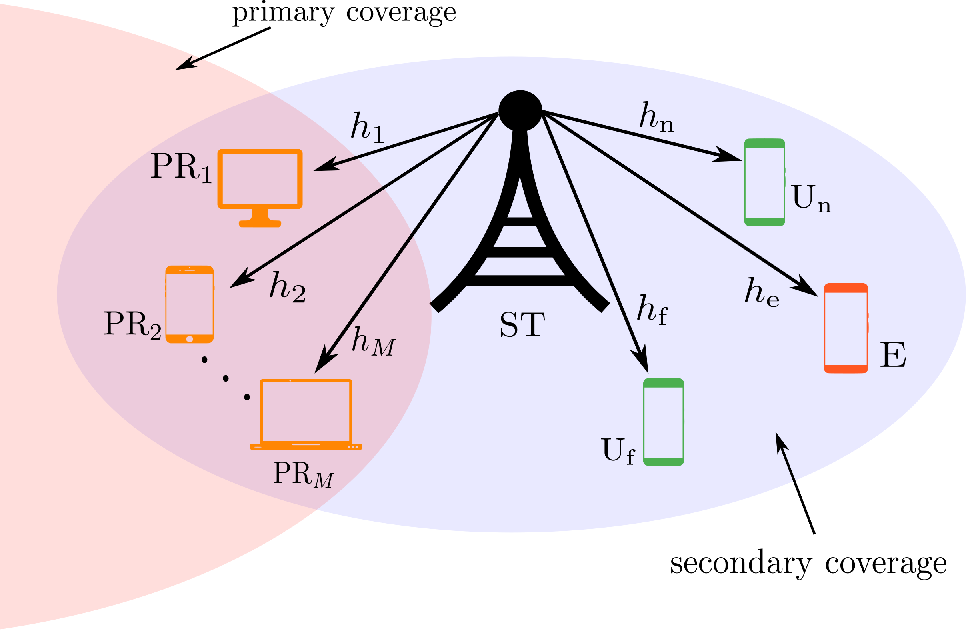
Fig. 1: System model for underlay spectrum sharing NOMA with multiple primary receivers.

Consider an underlay spectrum sharing system as shown in Fig. 1, consisting of MM PRs (PR1,PR2,…,PRM)\left(\mathrm{PR_{1},PR_{2},\ldots,PR}_{M}\right), one ST, two11 1 As suggested by the 3GPP-LTE, one resource block should be allocated for two NOMA users. Therefore, in this paper, we consider only two downlink NOMA users. Similar assumptions were considered in [7, 8, 9]. However, our analysis can be extended to multiple downlink NOMA users by adopting the user pairing scheme proposed in [9]. secondary (NOMA) receivers, denoted by Un\mathrm{U_{n}} (near user) and Uf\mathrm{U_{f}} (far user), and one eavesdropper E\mathrm{E}. It is assumed that all nodes are single-antenna devices. The distances of PRm​(m∈{1,2,…,M})\mathrm{PR}_{m}\left(m\in\left\{1,2,\ldots,M\right\}\right), Un\mathrm{U_{n}}, Uf\mathrm{U_{f}} and E\mathrm{E} from the ST are denoted by dm,dn,dfd_{m},d_{\mathrm{n}},d_{\mathrm{f}} and ded_{\mathrm{e}}, respectively. The channel fading coefficient for ST-PRm\mathrm{PR}_{m}, ST-Un\mathrm{U_{n}}, ST-Uf\mathrm{U_{f}} and ST-E\mathrm{E} links are, respectively, given by hm∼𝒞​𝒩​(0,Ωm=dm−α)h_{m}\sim\mathcal{CN}\left(0,\Omega_{m}=d_{m}^{-\alpha}\right), hn∼𝒞​𝒩​(0,Ωn=dn−α)h_{\mathrm{n}}\sim\mathcal{CN}\left(0,\Omega_{\mathrm{n}}=d_{\mathrm{n}}^{-\alpha}\right), hf∼𝒞​𝒩​(0,Ωf=df−α)h_{\mathrm{f}}\sim\mathcal{CN}\left(0,\Omega_{\mathrm{f}}=d_{\mathrm{f}}^{-\alpha}\right) and he∼𝒞​𝒩​(0,Ωe=de−α)h_{\mathrm{e}}\sim\mathcal{CN}\left(0,\Omega_{\mathrm{e}}=d_{\mathrm{e}}^{-\alpha}\right), with α\alpha denoting the path loss exponent. The corresponding channel gain is given by gi≜|hi|2,i∈{1,2,…,M,n,f,e}g_{i}\triangleq\left|h_{i}\right|^{2},i\in\left\{1,2,\ldots,M,\mathrm{n,f,e}\right\}. We assume that the ST has imperfect instantaneous CSI of the ST-PRm\mathrm{PR}_{m}, ST-Un\mathrm{U_{n}}, ST-Uf\mathrm{U_{f}} and ST-E\mathrm{E} links. Let the estimate of hih_{i} be denoted by h~i\tilde{h}_{i}, and hi=h~i+ϵih_{i}=\tilde{h}_{i}+\epsilon_{i}, where ϵi∼𝒞​𝒩​(0,σϵ2)\epsilon_{i}\sim\mathcal{CN}\left(0,\sigma_{\epsilon}^{2}\right) is the channel estimation error. Therefore, h~i∼𝒞​𝒩​(0,Ω~i)\tilde{h}_{i}\sim\mathcal{CN}\left(0,\tilde{\Omega}_{i}\right), where Ω~i=Ωi−σϵ2\tilde{\Omega}_{i}=\Omega_{i}-\sigma_{\epsilon}^{2} and the corresponding channel gain is denoted by g~i\tilde{g}_{i}. The peak (instantaneous) interference that the PRs can tolerate from the secondary network is denoted by IpI_{\mathrm{p}}, and the maximum transmit power at the ST is denoted by PmaxP_{\max}. Therefore, the instantaneous transmit power of the ST is given by P=min⁡{Pmax,Ipg~1,Ipg~2,…,Ipg~M}=min⁡{Pmax,Ipg~p}P=\min\left\{P_{\max},\tfrac{I_{\mathrm{p}}}{\tilde{g}_{1}},\tfrac{I_{\mathrm{p}}}{\tilde{g}_{2}},\ldots,\tfrac{I_{\mathrm{p}}}{\tilde{g}_{M}}\right\}=\min\left\{P_{\max},\tfrac{I_{\mathrm{p}}}{\tilde{g}_{\mathrm{p}}}\right\}, where g~p≜maxm⁡g~m\tilde{g}_{\mathrm{p}}\triangleq\max_{m}\tilde{g}_{m}. We denote the probability density function (PDF), cumulative distribution function (CDF) and complementary CDF (CCDF) of a random variable 𝒳\mathcal{X} by f𝒳​(⋅)f_{\mathcal{X}}\left(\cdot\right), F𝒳​(⋅)F_{\mathcal{X}}\left(\cdot\right) and ℱ𝒳​(⋅)\mathcal{F_{X}}\left(\cdot\right), respectively, and we define ℱ𝒳​(c1,c2)≜∫c1c2f𝒳​(t)​𝑑t\mathscr{F}_{\mathcal{X}}\left(c_{1},c_{2}\right)\triangleq\int_{c_{1}}^{c_{2}}f_{\mathcal{X}}\left(t\right)\mathrm{d}t.

III Analysis of the ESSR

Based on the estimated CSI at the ST, the users Un\mathrm{U_{n}} and Uf\mathrm{U_{f}} are further categorized as Us\mathrm{U_{s}} (strong user) and Uw\mathrm{U_{w}} (weak user), where s≜argmaxj∈{n,f}​g~j\mathrm{s}\triangleq\mathrm{argmax}_{j\in\left\{\mathrm{n,f}\right\}}\ \tilde{g}_{j} and w≜argminj∈{n,f}​g~j\mathrm{w}\triangleq\mathrm{argmin}_{j\in\left\{\mathrm{n,f}\right\}}\ \tilde{g}_{j}. The signal received at Uk,k∈{s,w}\mathrm{U}_{k},k\in\left\{\mathrm{s},\mathrm{w}\right\} is given by

yk=(h~k+ϵk)​(as​P​xs+aw​P​xw)+nk,y_{k}=\left(\tilde{h}_{k}+\epsilon_{k}\right)\left(\sqrt{a_{\mathrm{s}}P}x_{\mathrm{s}}+\sqrt{a_{\mathrm{w}}P}x_{\mathrm{w}}\right)+n_{k},

where xkx_{k} is the unit-energy information-bearing complex constellation symbol and nk∼𝒞​𝒩​(0,1)n_{k}\sim\mathcal{CN}\left(0,1\right) is the additive white Gaussian noise (AWGN) at node Uk\mathrm{U}_{k}. Following the NOMA principle, it is assumed that as<awa_{\mathrm{s}}<a_{\mathrm{w}} and as+aw=1a_{\mathrm{s}}+a_{\mathrm{w}}\mathrm{=1}. The weak user decodes xwx_{\mathrm{w}} by treating the interference due to xsx_{\mathrm{s}} as additional noise, whereas the strong user first decodes xwx_{\mathrm{w}} by treating the interference due to xsx_{\mathrm{s}} as additional noise and then applies successive interference cancellation (SIC) to decode xsx_{\mathrm{s}}. Therefore, the signal-to-interference-plus-noise ratio (SINR) at Us\mathrm{U_{s}} and Uw\mathrm{U_{w}} are, respectively, given by

γs=as​g~s​P1+σϵ2​P,γw=aw​g~w​P1+as​g~w​P+σϵ2​P.\gamma_{\mathrm{s}}=\dfrac{a_{\mathrm{s}}\tilde{g}_{\mathrm{s}}P}{1+\sigma_{\epsilon}^{2}P},\qquad\gamma_{\mathrm{w}}=\dfrac{a_{\mathrm{w}}\tilde{g}_{\mathrm{w}}P}{1+a_{\mathrm{s}}\tilde{g}_{\mathrm{w}}P+\sigma_{\epsilon}^{2}P}.

Following [13, Ch. 15], we consider the case that E\mathrm{E} follows the same decoding order as that of the legitimate users. Therefore, the SINR at E\mathrm{E} for decoding xwx_{\mathrm{w}} and xsx_{\mathrm{s}} are respectively given by

γe,w=aw​g~e​P1+as​g~e​P+σϵ2​P,γe,s=as​g~e​P1+σϵ2​P.\gamma_{\mathrm{e,w}}=\dfrac{a_{\mathrm{w}}\tilde{g}_{\mathrm{e}}P}{1+a_{\mathrm{s}}\tilde{g}_{\mathrm{e}}P+\sigma_{\epsilon}^{2}P},\qquad\gamma_{\mathrm{e,s}}=\dfrac{a_{\mathrm{s}}\tilde{g}_{\mathrm{e}}P}{1+\sigma_{\epsilon}^{2}P}.

Let g^s≜σϵ2+as​g~s\hat{g}_{\mathrm{s}}\triangleq\sigma_{\epsilon}^{2}+a_{\mathrm{s}}\tilde{g}_{\mathrm{s}}, g^w≜σϵ2+as​g~w\hat{g}_{\mathrm{w}}\triangleq\sigma_{\epsilon}^{2}+a_{\mathrm{s}}\tilde{g}_{\mathrm{w}}, gˇw≜σϵ2+g~w\check{g}_{\mathrm{w}}\triangleq\sigma_{\epsilon}^{2}+\tilde{g}_{\mathrm{w}} and g^e≜σϵ2+as​g~e\hat{g}_{\mathrm{e}}\triangleq\sigma_{\epsilon}^{2}+a_{\mathrm{s}}\tilde{g}_{\mathrm{e}}. Then using the standard statistical procedure of transformation of random variables, it follows that

fg^s​(x)=∑ℓ∈{1,2,3}A^ℓ​exp⁡(−xas​Ξℓ),ℱg^s​(x)=∑ℓ∈{1,2,3}𝒜^ℓ​exp⁡(−xas​Ξℓ),f_{\hat{g}_{\mathrm{s}}}\!\left(x\right)\!=\!\!\!\sum_{\ell\in\left\{1,2,3\right\}}\!\!\!\!\!\!\hat{A}_{\ell}\exp\!\left(\!\dfrac{-x}{a_{\mathrm{s}}\Xi_{\ell}}\!\right),\mathcal{F}_{\hat{g}_{\mathrm{s}}}\!\left(x\right)\!=\!\!\!\sum_{\ell\in\left\{1,2,3\right\}}\!\!\!\!\!\!\hat{\mathcal{A}}_{\ell}\exp\!\left(\!\dfrac{-x}{a_{\mathrm{s}}\Xi_{\ell}}\!\right),
fg^w​(x)=−A^2​exp⁡(−xas​Ξ2),ℱg^w​(x)=−𝒜^2​exp⁡(−xas​Ξ2),f_{\hat{g}_{\mathrm{w}}}\left(x\right)=-\hat{A}_{2}\exp\left(\dfrac{-x}{a_{\mathrm{s}}\Xi_{2}}\right),\mathcal{F}_{\hat{g}_{\mathrm{w}}}\left(x\right)=-\hat{\mathcal{A}}_{2}\exp\left(\dfrac{-x}{a_{\mathrm{s}}\Xi_{2}}\right),
fgˇw​(x)=Aˇ2​exp⁡(−xΞ2),ℱgˇw​(x)=𝒜ˇ2​exp⁡(−xΞ2),f_{\check{g}_{\mathrm{w}}}\left(x\right)=\check{A}_{2}\exp\left(\dfrac{-x}{\Xi_{2}}\right),\mathcal{F}_{\check{g}_{\mathrm{w}}}\left(x\right)=\check{\mathcal{A}}_{2}\exp\left(\dfrac{-x}{\Xi_{2}}\right),
fg^e​(x)=C^e​exp⁡(−xas​Ω~e),ℱg^e​(σϵ2,x)=1−𝒞^e​exp⁡(−xas​Ω~e),f_{\hat{g}_{\mathrm{e}}}\!\left(x\right)\!=\!\hat{C}_{\mathrm{e}}\exp\left(\!\dfrac{-x}{a_{\mathrm{s}}\tilde{\Omega}_{\mathrm{e}}}\!\right),\mathscr{F}_{\hat{g}_{\mathrm{e}}}\!\left(\sigma_{\epsilon}^{2},x\right)\!=1-\hat{\mathscr{C}}_{\mathrm{e}}\exp\left(\!\dfrac{-x}{a_{\mathrm{s}}\tilde{\Omega}_{\mathrm{e}}}\!\right),
ℱgˇe​(σϵ2,x)=1−𝒞ˇe​exp⁡(−xΩ~e),\mathscr{F}_{\check{g}_{\mathrm{e}}}\left(\sigma_{\epsilon}^{2},x\right)=1-\check{\mathscr{C}}_{\mathrm{e}}\exp\left(\dfrac{-x}{\tilde{\Omega}_{\mathrm{e}}}\right),

where Ξ1=Ω~n\Xi_{1}=\tilde{\Omega}_{\mathrm{n}}, Ξ2=Ω~n,f\Xi_{2}=\tilde{\Omega}_{\mathrm{n,f}}, Ξ3=Ω~f\Xi_{3}=\tilde{\Omega}_{\mathrm{f}}, Ω~n,f=(Ω~n−1+Ω~f−1)−1\tilde{\Omega}_{\mathrm{n,f}}=\left(\tilde{\Omega}_{\mathrm{n}}^{-1}+\tilde{\Omega}_{\mathrm{f}}^{-1}\right)^{-1}, A^ℓ=(−1)ℓ+1as​Ξℓ​exp⁡(σϵ2as​Ξℓ)\hat{A}_{\ell}=\tfrac{(-1)^{\ell+1}}{a_{\mathrm{s}}\Xi_{\ell}}\exp\left(\tfrac{\sigma_{\epsilon}^{2}}{a_{\mathrm{s}}\Xi_{\ell}}\right), 𝒜^ℓ=as​Ξℓ​A^ℓ\hat{\mathcal{A}}_{\ell}=a_{\mathrm{s}}\Xi_{\ell}\hat{A}_{\ell}, Aˇ2=1Ξ2​exp⁡(σϵ2Ξ2)\check{A}_{2}=\tfrac{1}{\Xi_{2}}\exp\left(\tfrac{\sigma_{\epsilon}^{2}}{\Xi_{2}}\right), 𝒜ˇ2=Ξ2​Aˇ2\check{\mathcal{A}}_{2}=\Xi_{2}\check{A}_{2}, C^e=1as​Ω~e​exp⁡(σϵ2as​Ω~e)\hat{C}_{\mathrm{e}}=\tfrac{1}{a_{\mathrm{s}}\tilde{\Omega}_{\mathrm{e}}}\exp\left(\tfrac{\sigma_{\epsilon}^{2}}{a_{\mathrm{s}}\tilde{\Omega}_{\mathrm{e}}}\right) and 𝒞^e=as​Ω~e​C^e\hat{\mathscr{C}}_{\mathrm{e}}=a_{\mathrm{s}}\tilde{\Omega}_{\mathrm{e}}\hat{C}_{\mathrm{e}}. From [14], the PDF of g~p\tilde{g}_{\mathrm{p}} is given by

fg~p(x)=−∑𝜼∈Φκ𝜼B𝜼exp(−B𝜼x),f_{\tilde{g}_{\mathrm{p}}}\left(x\right)=-\sum_{\boldsymbol{\eta}\in\Phi}\kappa_{\boldsymbol{\eta}}B_{\boldsymbol{\eta}}\exp\left(-B_{\boldsymbol{\eta}}x\right),

where Φ={𝜼=[η1η2⋯ηM]∈ℤ2M|∑m=1Mηm>0}\Phi=\left\{\boldsymbol{\eta}=[\eta_{1}\eta_{2}\cdots\eta_{M}]\in\mathbb{Z}_{2}^{M}\left|\sum\nolimits_{m=1}^{M}\eta_{m}>0\right.\right\} represents the set of all nonzero binary vectors of length MM, ℤ2={0,1}\mathbb{Z}_{2}=\left\{0,1\right\}, κ𝜼=∏m=1M(−1)ηm\kappa_{\boldsymbol{\eta}}=\prod_{m=1}^{M}(-1)^{\eta_{m}} and B𝜼=∑m=1M(ηm/Ω~m)B_{\boldsymbol{\eta}}=\sum_{m=1}^{M}\left(\eta_{m}/\tilde{\Omega}_{m}\right).

Finally, the ESR of the strong user can be written as

R¯s\displaystyle\bar{R}_{\mathrm{s}} =𝔼⁡{max⁡{log2⁡(1+γs)−log2⁡(1+γe,s),0}}\displaystyle=\mathbb{E}\left\{\max\left\{\log_{2}\left(1+\gamma_{\mathrm{s}}\right)-\log_{2}\left(1+\gamma_{\mathrm{e,s}}\right),0\right\}\right\}
=𝔼⁡{max⁡{log2⁡(1+g^s​P)−log2⁡(1+g^e​P),0}}.\displaystyle=\mathbb{E}\left\{\max\left\{\log_{2}\left(1+\hat{g}_{\mathrm{s}}P\right)-\log_{2}\left(1+\hat{g}_{\mathrm{e}}P\right),0\right\}\right\}. (1)
Theorem 1.

A closed-form expression for the ESR of Us\mathrm{U_{s}} can be derived as

R¯s=ℐs,1+ℐs,2−ℐs,3−ℐs,4,\bar{R}_{\mathrm{s}}=\mathscr{I}_{\mathrm{s,1}}+\mathscr{I}_{\mathrm{s,2}}-\mathscr{I}_{\mathrm{s,3}}-\mathscr{I}_{\mathrm{s,4}}, (2)

where the expressions for ℐs,1,ℐs,2,ℐs,3\mathscr{I}_{\mathrm{s,1}},\mathscr{I}_{\mathrm{s,2}},\mathscr{I}_{\mathrm{s,3}} and ℐs,4\mathscr{I}_{\mathrm{s,4}} are given by (3) – (6), shown at the top of the next page, Θ≜Ip/Pmax\Theta\triangleq I_{\mathrm{p}}/P_{\max}, Ξℓ,e≜(Ξℓ−1+Ω~−1)−1\Xi_{\ell,e}\triangleq\left(\Xi_{\ell}^{-1}+\tilde{\Omega}^{-1}\right)^{-1}, and Ei⁡(⋅)\mathrm{Ei}\left(\cdot\right) and E1​(⋅)\mathrm{E_{1}}\left(\cdot\right) are the exponential integrals.

ℐs,1=−log2⁡(e)​as​[∑ℓ∈{1,2,3}A^ℓ​{Ξℓ​𝕁1​(as​Ξℓ)−𝒞^e​Ξℓ,e​𝕁1​(as​Ξℓ,e)}]​[∑𝜼∈Φκ𝜼​{1−exp⁡(−B𝜼​Θ)}],\mathscr{I}_{\mathrm{s,1}}=-\log_{2}\left(e\right)a_{\mathrm{s}}\text{$\left[\sum_{\ell\in\left\{1,2,3\right\}}\hat{A}_{\ell}\left\{\Xi_{\ell}\mathbb{J}_{1}\left(a_{\mathrm{s}}\Xi_{\ell}\right)-\hat{\mathscr{C}}_{\mathrm{e}}\Xi_{\ell,\mathrm{e}}\mathbb{J}_{1}\left(a_{\mathrm{s}}\Xi_{\ell,\mathrm{e}}\right)\right\}\right]$}\left[\sum_{\boldsymbol{\eta}\in\Phi}\kappa_{\boldsymbol{\eta}}\left\{1-\exp\left(-B_{\boldsymbol{\eta}}\Theta\right)\right\}\right], (3)
ℐs,2=−log2(e)as∑ℓ∈{1,2,3}∑𝜼∈ΦA^ℓκη[Ξℓ𝕁2(asΞℓ)−𝒞^eΞℓ,e𝕁2(asΞℓ,e)],\mathscr{I}_{\mathrm{s,2}}=-\log_{2}\left(e\right)a_{\mathrm{s}}\sum_{\ell\in\left\{1,2,3\right\}}\sum_{\boldsymbol{\eta}\in\Phi}\hat{A}_{\ell}\kappa_{\eta}\left[\Xi_{\ell}\mathbb{J}_{2}\left(a_{\mathrm{s}}\Xi_{\ell}\right)-\hat{\mathscr{C}}_{\mathrm{e}}\Xi_{\ell,\mathrm{e}}\mathbb{J}_{2}\left(a_{\mathrm{s}}\Xi_{\ell,\mathrm{e}}\right)\right], (4)
ℐs,3=−log2⁡(e)​as​C^e​[∑ℓ∈{1,2,3}𝒜^ℓ​Ξℓ,e​𝕁1​(as​Ξℓ,e)]​[∑𝜼∈Φκ𝜼​{1−exp⁡(−B𝜼​Θ)}],\mathscr{I}_{\mathrm{s,3}}=-\log_{2}\left(e\right)a_{\mathrm{s}}\hat{C}_{\mathrm{e}}\left[\sum_{\ell\in\left\{1,2,3\right\}}\hat{\mathcal{A}}_{\ell}\Xi_{\ell,\mathrm{e}}\mathbb{J}_{1}\left(a_{\mathrm{s}}\Xi_{\ell,\mathrm{e}}\right)\right]\left[\sum_{\boldsymbol{\eta}\in\Phi}\kappa_{\boldsymbol{\eta}}\left\{1-\exp\left(-B_{\boldsymbol{\eta}}\Theta\right)\right\}\right], (5)
ℐs,4=−log2(e)asC^e∑ℓ∈{1,2,3}∑𝜼∈Φ𝒜^ℓκ𝜼Ξℓ,2𝕁2(asΞℓ,e),\mathscr{I}_{\mathrm{s,4}}=-\log_{2}\left(e\right)a_{\mathrm{s}}\hat{C}_{\mathrm{e}}\sum_{\ell\in\left\{1,2,3\right\}}\sum_{\boldsymbol{\eta}\in\Phi}\hat{\mathcal{A}}_{\ell}\kappa_{\boldsymbol{\eta}}\Xi_{\ell,2}\mathbb{J}_{2}\left(a_{\mathrm{s}}\Xi_{\ell,\mathrm{e}}\right), (6)
𝕁1​(Ω)=exp⁡(−σϵ2Ω)​ln⁡(1+σϵ2​Pmax)+exp⁡(1Ω​Pmax)​E1​[1Ω​(1Pmax+σϵ2)],\mathbb{J}_{1}\left(\Omega\right)=\exp\left(\dfrac{-\sigma_{\epsilon}^{2}}{\Omega}\right)\ln\left(1+\sigma_{\epsilon}^{2}P_{\max}\right)+\exp\left(\dfrac{1}{\Omega P_{\max}}\right)\mathrm{E}_{1}\left[\dfrac{1}{\Omega}\left(\dfrac{1}{P_{\max}}+\sigma_{\epsilon}^{2}\right)\right], (7)
𝕁2​(Ω)≜\displaystyle\mathbb{J}_{2}\left(\Omega\right)\triangleq exp(−σϵ2Ω)Ei(−B𝜼Θ)−B𝜼−1B𝜼−1−Ip​Ω{exp(Ipσϵ2B𝜼−σϵ2Ω)Ei(−B𝜼(Θ+Ipσϵ2))−exp(ΘIp​Ω−B𝜼Θ)\displaystyle\exp\left(\dfrac{-\sigma_{\epsilon}^{2}}{\Omega}\right)\mathrm{Ei}\left(-B_{\boldsymbol{\eta}}\Theta\right)-\dfrac{B_{\boldsymbol{\eta}}^{-1}}{B_{\boldsymbol{\eta}}^{-1}-I_{\mathrm{p}}\Omega}\left\{\exp\left(I_{\mathrm{p}}\sigma_{\epsilon}^{2}B_{\boldsymbol{\eta}}-\dfrac{\sigma_{\epsilon}^{2}}{\Omega}\right)\mathrm{Ei}\left(-B_{\boldsymbol{\eta}}\left(\Theta+I_{\mathrm{p}}\sigma_{\epsilon}^{2}\right)\right)-\exp\left(\dfrac{\Theta}{I_{\mathrm{p}}\Omega}-B_{\boldsymbol{\eta}}\Theta\right)\right.
×Ei(−Θ−Ip​σϵ2Ip​Ω)}+exp(−B𝜼Θ−σϵ2Ω){ln(1+Ip​σϵ2Θ)+exp(Θ+Ip​σϵ2Ip​Ω)E1(Θ+Ip​σϵ2Ip​Ω)}.\displaystyle\left.\times\mathrm{Ei}\left(\dfrac{-\Theta-I_{\mathrm{p}}\sigma_{\epsilon}^{2}}{I_{\mathrm{p}}\Omega}\right)\right\}+\exp\left(-B_{\boldsymbol{\eta}}\Theta-\dfrac{\sigma_{\epsilon}^{2}}{\Omega}\right)\left\{\ln\left(1+\dfrac{I_{\mathrm{p}}\sigma_{\epsilon}^{2}}{\Theta}\right)+\exp\left(\dfrac{\Theta+I_{\mathrm{p}}\sigma_{\epsilon}^{2}}{I_{\mathrm{p}}\Omega}\right)\mathrm{E}_{1}\left(\dfrac{\Theta+I_{\mathrm{p}}\sigma_{\epsilon}^{2}}{I_{\mathrm{p}}\Omega}\right)\right\}. (8)
 
Proof:

See Appendix A. ∎On the other hand, the ESR for the weak user Uw\mathrm{U_{w}} can be written as

R¯w=𝔼⁡{max⁡{log2⁡(1+γw)−log2⁡(1+γe,w),0}}\displaystyle\bar{R}_{\mathrm{w}}=\mathbb{E}\left\{\max\left\{\log_{2}\left(1+\gamma_{\mathrm{w}}\right)-\log_{2}\left(1+\gamma_{\mathrm{e,w}}\right),0\right\}\right\}
=𝔼{max{log2(1+(g~w+σϵ2)P1+(asg~w+σϵ2)P)\displaystyle=\mathbb{E}\left\{\max\left\{\log_{2}\left(\dfrac{1+\left(\tilde{g}_{{}_{\mathrm{w}}}+\sigma_{\epsilon}^{2}\right)P}{1+\left(a_{\mathrm{s}}\tilde{g}_{\mathrm{{}_{\mathrm{w}}}}+\sigma_{\epsilon}^{2}\right)P}\right)\right.\right.
−log2(1+(g~e+σϵ2)P1+(asg~e+σϵ2)P),0}}.\displaystyle\qquad\qquad\qquad-\left.\left.\log_{2}\left(\dfrac{1+\left(\tilde{g}_{{}_{\mathrm{e}}}+\sigma_{\epsilon}^{2}\right)P}{1+\left(a_{\mathrm{s}}\tilde{g}_{{}_{\mathrm{e}}}+\sigma_{\epsilon}^{2}\right)P}\right),0\right\}\right\}. (9)
Theorem 2.

A closed-form expression for the ESR of Uw\mathrm{U_{w}} can be derived as

R¯w=ℐw,1+ℐw,2−ℐw,3−ℐw,4,\bar{R}_{\mathrm{w}}=\mathscr{I}_{\mathrm{w,1}}+\mathscr{I}_{\mathrm{w,2}}-\mathscr{I}_{\mathrm{w,3}}-\mathscr{I}_{\mathrm{w,4}}, (10)

where the expressions for ℐw,1,ℐw,2,ℐw,3\mathscr{I}_{\mathrm{w,1}},\mathscr{I}_{\mathrm{w,2}},\mathscr{I}_{\mathrm{w,3}} and ℐw,4\mathscr{I}_{\mathrm{w,4}} are given by (11) – (14), shown on the next page.

ℐw,1=−log2(e)∑𝜼∈Φκ𝜼{−exp(−B𝜼Θ)}[Aˇ2Ξ2𝕁1(Ξ2)−Aˇ2𝒞ˇeΞ2,e𝕁1(Ξ2,e)+A^2asΞ2𝕁1(asΞ2)−A^2𝒞^easΞ2,e𝕁1(asΞ2,e)],\mathscr{I}_{\mathrm{w,1}}\!=\!-\log_{2}\left(e\right)\!\sum_{\boldsymbol{\eta}\in\Phi}\!\kappa_{\boldsymbol{\eta}}\left\{1\!-\!\exp\left(\!-B_{\boldsymbol{\eta}}\Theta\right)\right\}\!\!\left[\!\check{A}_{2}\Xi_{2}\mathbb{J}_{1}\!\left(\Xi_{2}\right)\!-\!\check{A}_{2}\check{\mathscr{C}}_{\mathrm{e}}\Xi_{2,\mathrm{e}}\mathbb{J}_{1}\!\left(\Xi_{2,\mathrm{e}}\right)\!+\!\hat{A}_{2}a_{\mathrm{s}}\Xi_{2}\mathbb{J}_{1}\!\left(a_{\mathrm{s}}\Xi_{2}\right)\!-\!\hat{A}_{2}\hat{\mathscr{C}}_{\mathrm{e}}a_{\mathrm{s}}\Xi_{2,\mathrm{e}}\mathbb{J}_{1}\!\left(a_{\mathrm{s}}\Xi_{2,\mathrm{e}}\right)\right], (11)
ℐw,2=−log2(e)∑𝜼∈Φκ𝜼[Aˇ2Ξ2𝕁2(Ξ2)−Aˇ2𝒞ˇeΞ2,e𝕁2(Ξ2,e)+A^2asΞ2𝕁2(asΞ2)−A^2𝒞^easΞ2,e𝕁2(asΞ2,e)],\mathscr{I}_{\mathrm{w,2}}=\!-\log_{2}\left(e\right)\sum_{\boldsymbol{\eta}\in\Phi}\kappa_{\boldsymbol{\eta}}\left[\check{A}_{2}\Xi_{2}\mathbb{J}_{2}\left(\Xi_{2}\right)\!-\!\check{A}_{2}\check{\mathscr{C}}_{\mathrm{e}}\Xi_{2,\mathrm{e}}\mathbb{J}_{2}\left(\Xi_{2,\mathrm{e}}\right)+\hat{A}_{2}a_{\mathrm{s}}\Xi_{2}\mathbb{J}_{2}\left(a_{\mathrm{s}}\Xi_{2}\right)-\hat{A}_{2}\hat{\mathscr{C}}_{\mathrm{e}}a_{\mathrm{s}}\Xi_{2,\mathrm{e}}\mathbb{J}_{2}\left(a_{\mathrm{s}}\Xi_{2,\mathrm{e}}\right)\right], (12)
ℐw,3=−log2(e)∑𝜼∈Φκ𝜼{1−exp(−B𝜼Θ)}[𝒜ˇ2CˇeΞ2,e𝕁1(Ξ2,e)+𝒜^2C^easΞ2,e𝕁1(asΞ2,e)],\mathscr{I}_{\mathrm{w,3}}=-\log_{2}\left(e\right)\sum_{\boldsymbol{\eta}\in\Phi}\kappa_{\boldsymbol{\eta}}\left\{1-\exp\left(-B_{\boldsymbol{\eta}}\Theta\right)\right\}\left[\check{\mathcal{A}}_{2}\check{C}_{\mathrm{e}}\Xi_{2,\mathrm{e}}\mathbb{J}_{1}\left(\Xi_{2,\mathrm{e}}\right)+\hat{\mathcal{A}}_{2}\hat{C}_{\mathrm{e}}a_{\mathrm{s}}\Xi_{2,\mathrm{e}}\mathbb{J}_{1}\left(a_{\mathrm{s}}\Xi_{2,\mathrm{e}}\right)\right], (13)
ℐw,4=−log2(e)∑𝜼∈Φκ𝜼[𝒜ˇ2CˇeΞ2,e𝕁2(Ξ2,e)+as𝒜^2C^eΞ2,e𝕁2(asΞ2,e)].\mathscr{I}_{\mathrm{w,4}}=-\log_{2}\left(e\right)\sum_{\boldsymbol{\eta}\in\Phi}\kappa_{\boldsymbol{\eta}}\left[\check{\mathcal{A}}_{2}\check{C}_{\mathrm{e}}\Xi_{2,\mathrm{e}}\mathbb{J}_{2}\left(\Xi_{2,\mathrm{e}}\right)+a_{\mathrm{s}}\hat{\mathcal{A}}_{2}\hat{C}_{\mathrm{e}}\Xi_{2,\mathrm{e}}\mathbb{J}_{2}\left(a_{\mathrm{s}}\Xi_{2,\mathrm{e}}\right)\right]. (14)
 
Proof:

See Appendix B. ∎Using (2) and (10), a closed-form expression for the ESSR of the NOMA system is given by R¯sum=R¯s+R¯w\bar{R}_{\mathrm{sum}}=\bar{R}_{\mathrm{s}}+\bar{R}_{\mathrm{w}}.

ESSR for OMA

For the case of an underlay spectrum sharing OMA system, the ST transmits P​xs\sqrt{P}x_{\mathrm{s}} to Us\mathrm{U_{s}} in the first time slot, and P​xw\sqrt{P}x_{\mathrm{w}} to Uw\mathrm{U_{w}} in the second time slot. For a fair comparison between the NOMA and OMA systems, we consider the same value of IpI_{\mathrm{p}} for both systems. Therefore, the ESSR for the OMA system is given by

R¯sum,OMA=R¯s,OMA+R¯w,OMA\displaystyle\bar{R}_{\mathrm{sum,OMA}}=\bar{R}_{\mathrm{s,OMA}}+\bar{R}_{\mathrm{w,OMA}}
=∑k∈{s,w}𝔼⁡{0.5​max⁡{log2⁡(1+g~k​P1+g~e​P),0}}.\displaystyle=\sum_{k\in\left\{\mathrm{s,w}\right\}}\mathbb{E}\left\{0.5\max\left\{\log_{2}\left(\dfrac{1+\tilde{g}_{k}P}{1+\tilde{g}_{\mathrm{e}}P}\right),0\right\}\right\}. (15)

As the focus of this paper is on the NOMA-based system, we do not provide the closed-form expression for R¯sum,OMA\bar{R}_{\mathrm{sum,OMA}}. Next, we carry out the asymptotic analysis (Ip→∞)\left(I_{\mathrm{p}}\to\infty\right) of the ESSR for the NOMA system.

IV Asymptotic ESSR for the NOMA System

Theorem 3.

An analytical expression for the asymptotic (Ip→∞)\left(I_{\mathrm{p}}\to\infty\right) ESSR for the NOMA system can be derived as

R¯sum,asymp=ℐs+ℐw,\bar{R}_{\mathrm{sum,asymp}}=\mathcal{I}_{\mathrm{s}}+\mathcal{I}_{\mathrm{w}}, (16)

where the closed-form expressions for ℐs\mathcal{I}_{\mathrm{s}} and ℐw\mathcal{I}_{\mathrm{w}} are given by (17) and (18), respectively, shown on the next page.

ℐs=log2⁡(e)​as​∑ℓ∈{1,2,3}[A^ℓ​Ξℓ​𝕁1​(as​Ξℓ)−A^ℓ​𝒞^e​Ξℓ,e​𝕁1​(as​Ξℓ,e)−𝒜^ℓ​C^e​Ξℓ,e​𝕁1​(as​Ξℓ,e)],\displaystyle\mathcal{I}_{\mathrm{s}}=\log_{2}\left(e\right)a_{\mathrm{s}}\sum_{\ell\in\left\{1,2,3\right\}}\left[\hat{A}_{\ell}\Xi_{\ell}\mathbb{J}_{1}\left(a_{\mathrm{s}}\Xi_{\ell}\right)-\hat{A}_{\ell}\hat{\mathscr{C}}_{\mathrm{e}}\Xi_{\ell,\mathrm{e}}\mathbb{J}_{1}\left(a_{\mathrm{s}}\Xi_{\ell,\mathrm{e}}\right)-\hat{\mathcal{A}}_{\ell}\hat{C}_{\mathrm{e}}\Xi_{\ell,\mathrm{e}}\mathbb{J}_{1}\left(a_{\mathrm{s}}\Xi_{\ell,\mathrm{e}}\right)\right], (17)
ℐw=log2(e)[Aˇ2Ξ2𝕁1(Ξ2)−Aˇ2𝒞ˇeΞ2,e𝕁1(Ξ2,e)+A^2asΞ2𝕁1(asΞ2)−A^2𝒞^easΞ2,e𝕁1(asΞ2,e)\displaystyle\mathcal{I}_{\mathrm{w}}=\log_{2}\left(e\right)\left[\check{A}_{2}\Xi_{2}\mathbb{J}_{1}\!\left(\Xi_{2}\right)\!-\!\check{A}_{2}\check{\mathscr{C}}_{\mathrm{e}}\Xi_{2,\mathrm{e}}\mathbb{J}_{1}\!\left(\Xi_{2,\mathrm{e}}\right)\!+\!\hat{A}_{2}a_{\mathrm{s}}\Xi_{2}\mathbb{J}_{1}\!\left(a_{\mathrm{s}}\Xi_{2}\right)\!-\!\hat{A}_{2}\hat{\mathscr{C}}_{\mathrm{e}}a_{\mathrm{s}}\Xi_{2,\mathrm{e}}\mathbb{J}_{1}\!\left(a_{\mathrm{s}}\Xi_{2,\mathrm{e}}\right)\right.
−𝒜ˇ2CˇeΞ2,e𝕁1(Ξ2,e)−𝒜^2C^easΞ2,e𝕁1(asΞ2,e)].\displaystyle\qquad\qquad\qquad\qquad\qquad\qquad\qquad\qquad\qquad\qquad\qquad\qquad-\left.\check{\mathcal{A}}_{2}\check{C}_{\mathrm{e}}\Xi_{2,\mathrm{e}}\mathbb{J}_{1}\left(\Xi_{2,\mathrm{e}}\right)-\hat{\mathcal{A}}_{2}\hat{C}_{\mathrm{e}}a_{\mathrm{s}}\Xi_{2,\mathrm{e}}\mathbb{J}_{1}\left(a_{\mathrm{s}}\Xi_{2,\mathrm{e}}\right)\right]. (18)
 
Proof:

Note that for Ip→∞I_{\mathrm{p}}\to\infty and finite PmaxP_{\max}, we have Θ=IPPmax→∞\Theta=\tfrac{I_{\mathrm{P}}}{P_{\max}}\to\infty. Letting Θ→∞\Theta\to\infty in (19) and (25), and then solving the integrals following a similar line of argument as given in Appendix A, a closed-form expression for R¯sum,asymp\bar{R}_{\mathrm{sum,asymp}} is given by (16). This concludes the proof. ∎It can be noted from (16) – (18) that for large values of IpI_{\mathrm{p}}, the ESSR of the NOMA is independent of the number of PRs as well as the quality of the link between the ST and PRs. Also, the slope of the ESSR w.r.t IpI_{\mathrm{p}} becomes equal to zero for Ip→∞I_{\mathrm{p}}\to\infty.

Refer to caption
Fig. 2: Comparison of ESR for NOMA and OMA systems for Pmax=50P_{\max}=50 dB.
Refer to caption
Fig. 3: Comparison of ESSR for NOMA and OMA systems. The number in the parentheses denotes PmaxP_{\max} in dB.
Refer to caption
Fig. 4: Effect of channel estimation error on the ESSR. The numbers in the parentheses denote (Ip,Pmax)\left(I_{\mathrm{p}},P_{\max}\right) in dB.
Refer to caption
Fig. 5: Effect of the number of PRs on the ESSR of the NOMA system. The number in the parentheses denotes PmaxP_{\max} in dB.

V Results and Discussions

In this section, we present the numerical and analytical results for the ESSR of NOMA and OMA systems. We consider a system with dn=30d_{\mathrm{n}}=30 m, df=100d_{\mathrm{f}}=100 m, de=150d_{\mathrm{e}}=150 m, {d1,d2,d3,d4}={200,205,210,215}\left\{d_{1},d_{2},d_{3},d_{4}\right\}=\left\{200,205,210,215\right\} m, σϵ2=2×10⁻⁵\sigma_{\epsilon}^{2}=2\times 10^{-5}, and α=2\alpha=2, unless stated otherwise. In the case of NOMA, we use the bisection method to find the value of asa_{\mathrm{s}} such that R¯s=R¯s,OMA\bar{R}_{\mathrm{s}}=\bar{R}_{\mathrm{s,OMA}}, and then the remaining power fraction (aw)\left(a_{\mathrm{w}}\right) is allocated to the weak user. In each figure, the legend indicates the numerically obtained results, while the solid curves indicate the analytical results.

Fig. 2 shows a performance comparison of the ESR of the NOMA and OMA systems. It can be observed from the figure that the ESR of Us\mathrm{U_{s}} in the NOMA system is equal to that in the case of the OMA system (by virtue of the power allocation scheme), whereas the ESR of Uw\mathrm{U_{w}} in the NOMA system is higher that that of the OMA system. This result confirms that NOMA helps in maintaining the secrecy rate of the strong user while significantly enhancing the secrecy performance of the weak user as compared to OMA. We also show the asymptotic (Ip→∞)\left(I_{\mathrm{p}}\to\infty\right) ESR for the NOMA system, which matches well with the exact ESR for large IpI_{\mathrm{p}}. Moreover, a close agreement between the numerical and analytical results (for the case of NOMA) verifies the correctness of the derived closed-form expressions.

Fig. 3 shows a comparison of the ESSR for the NOMA and OMA systems. Note that the NOMA system outperforms its OMA-based counterpart by achieving a significantly higher ESSR. The ESSR for the NOMA/OMA system first increases with an increase of the value of IpI_{\mathrm{p}} (which we refer to the interference-constrained regime) and then saturates for larger value of IpI_{\mathrm{p}} (which we refer to as the power-constrained regime). Interestingly, in the interference-constrained regime, the ESSR of the NOMA system remains the same irrespective of the value of PmaxP_{\max}, whereas, in the power-constrained regime, the ESSR is independent of the value of IpI_{\mathrm{p}}. A similar behavior is evident for the OMA system. It is noteworthy that for the system parameters considered in Fig. 3, min⁡(Pmax,Ip𝔼​{g~p})=min⁡(Pmax,IpΩ~p)\min\left(P_{\max},\tfrac{I_{\mathrm{p}}}{\mathbb{E}\left\{\tilde{g}_{\mathrm{p}}\right\}}\right)=\min\left(P_{\max},\tfrac{I_{\mathrm{p}}}{\tilde{\Omega}_{\mathrm{p}}}\right) becomes constant (=Pmax)\left(=P_{\max}\right) w.r.t IpI_{p} at Ip≳0I_{\mathrm{p}}\gtrsim 0 dB for Pmax=40P_{\max}=40 dB, at Ip≳10I_{\mathrm{p}}\gtrsim 10 dB for Pmax=50P_{\max}=50 dB, and at Ip≳20I_{\mathrm{p}}\gtrsim 20 dB for Pmax=60P_{\max}=60 dB. Therefore, the ESSR for both the NOMA and OMA systems becomes constant w.r.t. IpI_{\mathrm{p}} (power-constrained regime) at Ip≳{0,10,20}I_{\mathrm{p}}\gtrsim\left\{0,10,20\right\} dB for Pmax={40,50,60}P_{\max}=\left\{40,50,60\right\} dB.

In Fig. 4, we investigate the effect of channel estimation error on the ESSR of the NOMA and OMA systems. It can be noted from the figure that the ESSR for both the NOMA and OMA systems decreases with an increase in the value of σϵ2\sigma_{\epsilon}^{2}. This implies that a decrease in the accuracy of channel estimation has an adverse effect on the system performance. The effect of the interference-constrained regime is also clearly evident from the figure, as the value of ESSR at Ip=0I_{\mathrm{p}}=0 dB is the same for Pmax=50P_{\max}=50 dB and Pmax=60P_{\max}=60 dB. However, for a large value of IpI_{\mathrm{p}} (10 dB), the benefit of a larger PmaxP_{\max} can be noted from the figure.

Fig. 5 shows the effect of the number and distance of PRs on the ESSR of the NOMA system. In this figure, three different cases are studied. In Case I, we consider 2 PRs both located at a distance of 200 m from the ST; in Case II, we consider 4 PRs located at {200,205,210,215}\left\{200,205,210,215\right\} m from the ST, and in Case III, we consider 10 PRs, all located at a distance of 200 m. Moreover, for all of the cases, we consider two different values of transmit power: Pmax=40P_{\max}=40 dB and 60 dB. It is evident from the figure that in the interference-constrained regime (i.e., for small values of IpI_{\mathrm{p}}), an increase in the number of PRs results in a reduction of the ESSR. However, in this regime, no benefit is observed from a higher PmaxP_{\max} budget. On the other hand, in the power-constrained regime (i.e., for large values of IpI_{p}), the ESSR for all the cases becomes the same, irrespective of the number/location of PRs. This occurs due to the reason that in the power-constrained regime, the secrecy performance becomes independent of the ST-PR link quality as well as the interference constraint at the PRs. However, a larger PmaxP_{\max} turns out to be clearly beneficial in this regime.

VI Conclusion

In this paper, we have presented the ergodic secrecy rate analysis of a two-user downlink NOMA system in an underlay spectrum sharing scenario consisting of multiple primary-user receivers in the presence of channel estimation error. Exact and asymptotic closed-form expressions for the ESSR of the NOMA system were derived. Our results confirmed that the NOMA system outperforms its OMA-based counterpart in terms of the ESSR. More interestingly, the results confirmed that no benefit is obtained in terms of the ESSR from a higher power budget at the ST in the interference-constrained regime, whereas, in the power-constrained regime, the ESSR becomes independent of the number of PRs as well as the quality of the ST-PR links. The results also showed that a larger channel estimation error results in a reduced secrecy rate. Finally, the asymptotic analysis demonstrated that the ESSR of the NOMA system becomes independent of the value of peak tolerable interference and therefore, the slope of the ESSR w.r.t. the peak tolerable interference becomes zero.

Appendix A Proof of Theorem 1

Using (1), we have

R¯s=𝔼⁡{max⁡{log2⁡(1+g^s​P)−log2⁡(1+g^e​P),0}}\displaystyle\bar{R}_{\mathrm{s}}=\mathbb{E}\left\{\max\left\{\log_{2}\left(1+\hat{g}_{\mathrm{s}}P\right)-\log_{2}\left(1+\hat{g}_{\mathrm{e}}P\right),0\right\}\right\}
=\displaystyle= ∫y=0Θ∫x=σϵ2∞log2⁡(+Pmax​x)​fg^s​(x)​ℱg^e​(σϵ2,x)​fg~p​(y)​𝑑x​𝑑y\displaystyle\int_{y=0}^{\Theta}\int_{x=\sigma_{\epsilon}^{2}}^{\infty}\!\!\!\!\log_{2}\left(1\!+\!P_{\max}x\right)f_{\hat{g}_{\mathrm{s}}}\!\left(x\right)\mathscr{F}_{\hat{g}_{\mathrm{e}}}\!\left(\sigma_{\epsilon}^{2},x\right)f_{\tilde{g}_{\mathrm{p}}}\!\left(y\right)\mathrm{d}x\mathrm{d}y
+\displaystyle+ ∫y=Θ∞∫x=σϵ2∞log2⁡(+Ip​xy)​fg^s​(x)​ℱg^e​(σϵ2,x)​fg~p​(y)​𝑑x​𝑑y\displaystyle\int_{y=\Theta}^{\infty}\int_{x=\sigma_{\epsilon}^{2}}^{\infty}\!\!\!\!\log_{2}\left(1\!+\!I_{\mathrm{p}}\dfrac{x}{y}\right)f_{\hat{g}_{\mathrm{s}}}\!\left(x\right)\mathscr{F}_{\hat{g}_{\mathrm{e}}}\!\left(\sigma_{\epsilon}^{2},x\right)f_{\tilde{g}_{\mathrm{p}}}\!\left(y\right)\mathrm{d}x\mathrm{d}y
−\displaystyle- ∫y=0Θ∫x=σϵ2∞log2⁡(1+Pmax​x)​fg^e​(x)​ℱg^s​(x)​fg~p​(y)​𝑑x​𝑑y\displaystyle\int_{y=0}^{\Theta}\int_{x=\sigma_{\epsilon}^{2}}^{\infty}\!\!\log_{2}\left(1+P_{\max}x\right)f_{\hat{g}_{\mathrm{e}}}\left(x\right)\mathcal{F}_{\hat{g}_{\mathrm{s}}}\left(x\right)f_{\tilde{g}_{\mathrm{p}}}\left(y\right)\mathrm{d}x\mathrm{d}y
−\displaystyle- ∫y=Θ∞∫x=σϵ2∞log2⁡(1+Ip​xy)​fg^e​(x)​ℱg^s​(x)​fg~p​(y)​𝑑x​𝑑y\displaystyle\int_{y=\Theta}^{\infty}\int_{x=\sigma_{\epsilon}^{2}}^{\infty}\!\!\log_{2}\left(1+I_{\mathrm{p}}\dfrac{x}{y}\right)f_{\hat{g}_{\mathrm{e}}}\left(x\right)\mathcal{F}_{\hat{g}_{\mathrm{s}}}\left(x\right)f_{\tilde{g}_{\mathrm{p}}}\left(y\right)\mathrm{d}x\mathrm{d}y
≜\displaystyle\triangleq ℐs,1+ℐs,2−ℐs,3−ℐs,4.\displaystyle\mathscr{I}_{\mathrm{s,1}}+\mathscr{I}_{s,2}-\mathscr{I}_{s,3}-\mathscr{I}_{s,4}. (19)

Solving for ℐs,1\mathscr{I}_{\mathrm{s,1}}, using the expressions for fg^s​(x),ℱg^e​(σϵ2,x)f_{\hat{g}_{\mathrm{s}}}\left(x\right),\mathscr{F}_{\hat{g}_{\mathrm{e}}}\left(\sigma_{\epsilon}^{2},x\right) and fg~p​(y)f_{\tilde{g}_{\mathrm{p}}}\left(y\right) yields

ℐs,1=−log2(e)∑ℓ∈{1,2,3}∑𝜼∈ΦA^ℓB𝜼κ𝜼\displaystyle\mathscr{I}_{\mathrm{s,1}}=-\log_{2}\left(e\right)\sum_{\ell\in\left\{1,2,3\right\}}\sum_{\boldsymbol{\eta}\in\Phi}\hat{A}_{\ell}B_{\boldsymbol{\eta}}\kappa_{\boldsymbol{\eta}}
×\displaystyle\times [∫y=0Θ∫x=σϵ2∞ln(+Pmaxx)exp(−xas​Ξℓ)exp(−B𝜼y)dxdy\displaystyle\left[\int_{y=0}^{\Theta}\int_{x=\sigma_{\epsilon}^{2}}^{\infty}\!\!\ln\left(1\!+\!P_{\max}x\right)\exp\!\left(\!\dfrac{-x}{a_{\mathrm{s}}\Xi_{\ell}}\!\right)\exp\left(-B_{\boldsymbol{\eta}}y\right)\mathrm{d}x\mathrm{d}y\right.
−\displaystyle- 𝒞^e∫y=0Θ∫x=σϵ2∞ln(+Pmaxx)exp(−xas​Ξℓ,e)exp(−B𝜼y)dxdy]\displaystyle\left.\hat{\mathscr{C}}_{\mathrm{e}}\!\!\int_{y=0}^{\Theta}\!\int_{x=\sigma_{\epsilon}^{2}}^{\infty}\!\!\!\!\!\ln\left(1\!+\!P_{\max}x\right)\exp\!\left(\!\dfrac{-x}{a_{\mathrm{s}}\Xi_{\ell,\mathrm{e}}}\!\right)\!\exp\left(-B_{\boldsymbol{\eta}}y\right)\mathrm{d}x\mathrm{d}y\right]
=\displaystyle= −log2(e)∑ℓ∈{1,2,3}∑𝜼∈ΦA^ℓκ𝜼{1−exp(−B𝜼Θ)}\displaystyle-\log_{2}\left(e\right)\sum_{\ell\in\left\{1,2,3\right\}}\sum_{\boldsymbol{\eta}\in\Phi}\hat{A}_{\ell}\kappa_{\boldsymbol{\eta}}\left\{1-\exp\left(-B_{\boldsymbol{\eta}}\Theta\right)\right\}
×[∫x=σϵ2∞ln(+Pmaxx)exp(−xas​Ξℓ)dx\displaystyle\qquad\times\left[\int_{x=\sigma_{\epsilon}^{2}}^{\infty}\!\!\ln\left(1\!+\!P_{\max}x\right)\exp\!\left(\!\dfrac{-x}{a_{\mathrm{s}}\Xi_{\ell}}\!\right)\mathrm{d}x\right.
−𝒞^e∫x=σϵ2∞ln(+Pmaxx)exp(−xas​Ξℓ,e)dx].\displaystyle\qquad-\left.\hat{\mathscr{C}}_{\mathrm{e}}\int_{x=\sigma_{\epsilon}^{2}}^{\infty}\!\!\ln\left(1\!+\!P_{\max}x\right)\exp\!\left(\!\dfrac{-x}{a_{\mathrm{s}}\Xi_{\ell,\mathrm{e}}}\!\right)\mathrm{d}x\right]. (20)

Computing the integrals above using integration by parts and with some algebraic manipulations, we arrive at the closed-form expression for ℐs,1\mathscr{I}_{\mathrm{s,1}} is given by (3). Similarly, for ℐs,3\mathscr{I}_{\mathrm{s,3}}, we have

ℐs,3=−log2(e)C^e∑ℓ∈{1,2,3}∑𝜼∈Φ𝒜^ℓB𝜼κ𝜼\displaystyle\mathscr{I}_{\mathrm{s,3}}=-\log_{2}\left(e\right)\hat{C}_{\mathrm{e}}\sum_{\ell\in\left\{1,2,3\right\}}\sum_{\boldsymbol{\eta}\in\Phi}\hat{\mathcal{A}}_{\ell}B_{\boldsymbol{\eta}}\kappa_{\boldsymbol{\eta}}
×∫y=0Θ∫x=σϵ2∞ln⁡(+Pmax​x)​exp⁡(−xas​Ξℓ,e)​exp⁡(−B𝜼​y)​𝑑x​𝑑y\displaystyle\times\int_{y=0}^{\Theta}\int_{x=\sigma_{\epsilon}^{2}}^{\infty}\!\!\!\!\ln\left(1\!+\!P_{\max}x\right)\exp\left(\!\dfrac{-x}{a_{\mathrm{s}}\Xi_{\ell,\mathrm{e}}}\!\right)\exp\left(-B_{\boldsymbol{\eta}}y\right)\mathrm{d}x\mathrm{d}y
=−log2(e)C^e∑ℓ∈{1,2,3}∑𝜼∈Φ𝒜^ℓκ𝜼{1−exp(−B𝜼Θ)}\displaystyle=-\log_{2}\left(e\right)\hat{C}_{\mathrm{e}}\sum_{\ell\in\left\{1,2,3\right\}}\sum_{\boldsymbol{\eta}\in\Phi}\hat{\mathcal{A}}_{\ell}\kappa_{\boldsymbol{\eta}}\left\{1-\exp\left(-B_{\boldsymbol{\eta}}\Theta\right)\right\}
×∫x=σϵ2∞ln⁡(+Pmax​x)​exp⁡(−xas​Ξℓ,e)​dx.\displaystyle\qquad\qquad\times\int_{x=\sigma_{\epsilon}^{2}}^{\infty}\!\!\ln\left(1\!+\!P_{\max}x\right)\exp\left(\!\dfrac{-x}{a_{\mathrm{s}}\Xi_{\ell,\mathrm{e}}}\!\right)\mathrm{dx}. (21)

A closed-form expression for (21) can be obtained by following the steps similar to those used to obtain ℐs,1\mathscr{I}_{\mathrm{s,1}}, and is given in (5). Now solving for ℐs,4\mathscr{I}_{\mathrm{s,4}}, we have

ℐs,4=−log2(e)C^e∑ℓ∈{1,2,3}∑𝜼∈Φ𝒜^ℓB𝜼κ𝜼∫y=Θ∞\displaystyle\mathscr{I}_{s,4}=-\log_{2}\left(e\right)\hat{C}_{\mathrm{e}}\sum_{\ell\in\left\{1,2,3\right\}}\sum_{\boldsymbol{\eta}\in\Phi}\hat{\mathcal{A}}_{\ell}B_{\boldsymbol{\eta}}\kappa_{\boldsymbol{\eta}}\int_{y=\Theta}^{\infty}
[∫x=σϵ2∞ln⁡(1+Ipy​x)​exp⁡(−xas​Ξℓ,e)​𝑑x]​exp⁡(−B𝜼​y)​𝑑y.\displaystyle\left[\int_{x=\sigma_{\epsilon}^{2}}^{\infty}\ln\left(1+\dfrac{I_{\mathrm{p}}}{y}x\right)\exp\left(\dfrac{-x}{a_{\mathrm{s}}\Xi_{\ell,\mathrm{e}}}\right)\mathrm{d}x\right]\exp\left(-B_{\boldsymbol{\eta}}y\right)\mathrm{d}y. (22)

Integrating the preceding expression w.r.t. xx using integration by parts and using a few algebraic manipulations yields

ℐs,4=−log2(e)C^e∑ℓ∈{1,2,3}∑𝜼∈Φ𝒜^ℓB𝜼κ𝜼asΞℓ,e∫y=Θ∞\displaystyle\mathscr{I}_{\mathrm{s,4}}=-\log_{2}\left(e\right)\hat{C}_{\mathrm{e}}\sum_{\ell\in\left\{1,2,3\right\}}\sum_{\boldsymbol{\eta}\in\Phi}\hat{\mathcal{A}}_{\ell}B_{\boldsymbol{\eta}}\kappa_{\boldsymbol{\eta}}a_{\mathrm{s}}\Xi_{\ell,\mathrm{e}}\int_{y=\Theta}^{\infty}
×[exp(−σϵ2as​Ξℓ,e)ln(1+Ip​σϵ2y)+exp(yas​Ip​Ξℓ,e)\displaystyle\times\left[\exp\left(\dfrac{-\sigma_{\epsilon}^{2}}{a_{\mathrm{s}}\Xi_{\ell,\mathrm{e}}}\right)\ln\left(1+\dfrac{I_{\mathrm{p}}\sigma_{\epsilon}^{2}}{y}\right)+\exp\left(\dfrac{y}{a_{\mathrm{s}}I_{\mathrm{p}}\Xi_{\ell,\mathrm{e}}}\right)\right.
×E1(1as​Ξℓ,e(yIp+σϵ2))]exp(−B𝜼y)dy.\displaystyle\left.\times\mathrm{E}_{1}\left(\dfrac{1}{a_{\mathrm{s}}\Xi_{\ell,\mathrm{e}}}\left(\dfrac{y}{I_{\mathrm{p}}}+\sigma_{\epsilon}^{2}\right)\right)\right]\exp\left(-B_{\boldsymbol{\eta}}y\right)\mathrm{d}y. (23)

Now solving the integral in (23) w.r.t yy using integration by parts, a closed-form expression for ℐs,4\mathscr{I}_{\mathrm{s,4}} is given in (6). Next, for ℐs,2,\mathscr{I}_{\mathrm{s,2}}, we have

ℐs,2=−log2(e)∑ℓ∈{1,2,3}∑𝜼∈ΦA^ℓB𝜼κ𝜼∫y=Θ∞∫x=σϵ2∞ln(1+Ipyx)\displaystyle\mathscr{I}_{\mathrm{s,}2}\!=\!-\log_{2}\left(e\right)\!\!\!\sum_{\ell\in\left\{1,2,3\right\}}\!\sum_{\boldsymbol{\eta}\in\Phi}\!\hat{A}_{\ell}B_{\boldsymbol{\eta}}\kappa_{\boldsymbol{\eta}}\int_{y=\Theta}^{\infty}\int_{x=\sigma_{\epsilon}^{2}}^{\infty}\!\!\!\ln\left(\!1+\dfrac{I_{\mathrm{p}}}{y}x\!\right)
×exp⁡(−xas​Ξℓ)​{1−𝒞^e​exp⁡(−xas​Ω~e)}​exp⁡(−B𝜼​y)​d​x​d​y.\displaystyle\times\exp\left(\dfrac{-x}{a_{\mathrm{s}}\Xi_{\ell}}\right)\left\{1-\hat{\mathscr{C}}_{\mathrm{e}}\exp\left(\dfrac{-x}{a_{\mathrm{s}}\tilde{\Omega}_{\mathrm{e}}}\right)\right\}\exp\left(-B_{\boldsymbol{\eta}}y\right)\mathrm{d}x\mathrm{d}y. (24)

Solving the integrals above by following the steps similar to those used for ℐs,4\mathscr{I}_{\mathrm{s,4}}, a closed-form expression for ℐs,2\mathscr{I}_{\mathrm{s,2}} is given by (4). This concludes the proof.

Appendix B Proof of Theorem 2

Using (9), we have

R¯w=𝔼{max{log2(1+(g~w+σϵ2)P1+(asg~w+σϵ2)P)\displaystyle\bar{R}_{\mathrm{w}}=\mathbb{E}\left\{\max\left\{\log_{2}\left(\dfrac{1+\left(\tilde{g}_{{}_{\mathrm{w}}}+\sigma_{\epsilon}^{2}\right)P}{1+\left(a_{\mathrm{s}}\tilde{g}_{\mathrm{{}_{\mathrm{w}}}}+\sigma_{\epsilon}^{2}\right)P}\right)\right.\right.
−log2(1+(g~e+σϵ2)P1+(asg~e+σϵ2)P),0}}\displaystyle\qquad\qquad\qquad-\left.\left.\log_{2}\left(\dfrac{1+\left(\tilde{g}_{{}_{\mathrm{e}}}+\sigma_{\epsilon}^{2}\right)P}{1+\left(a_{\mathrm{s}}\tilde{g}_{{}_{\mathrm{e}}}+\sigma_{\epsilon}^{2}\right)P}\right),0\right\}\right\}
=[∫y=0Θ∫x=σϵ2∞log2(+xPmax)fgˇw(x)ℱgˇe(x)fg~p(y)dxdy\displaystyle=\left[\int_{y=0}^{\Theta}\int_{x=\sigma_{\epsilon}^{2}}^{\infty}\!\!\!\!\!\log_{2}\left(1\!+\!xP_{\max}\right)f_{\check{g}_{{}_{\mathrm{w}}}}\!\left(x\right)\mathscr{F}_{\check{g}_{{}_{\mathrm{e}}}}\!\left(x\right)f_{\tilde{g}_{{}_{\mathrm{p}}}}\!\left(y\right)\mathrm{d}x\mathrm{d}y\right.
−∫y=0Θ∫x=σϵ2∞log2(+xPmax)fg^w(x)ℱg^e(x)fg~p(y)dxdy]\displaystyle\left.-\int_{y=0}^{\Theta}\int_{x=\sigma_{\epsilon}^{2}}^{\infty}\!\!\!\!\!\log_{2}\left(1\!+\!xP_{\max}\right)f_{\hat{g}_{{}_{\mathrm{w}}}}\!\left(x\right)\mathscr{F}_{\hat{g}_{{}_{\mathrm{e}}}}\!\left(x\right)f_{\tilde{g}_{{}_{\mathrm{p}}}}\!\left(y\right)\mathrm{d}x\mathrm{d}y\right]
+[∫y=Θ∞∫x=σϵ2∞log2(1+Ipxy)fgˇw(x)ℱgˇe(x)fg~p(y)dxdy\displaystyle+\left[\int_{y=\Theta}^{\infty}\int_{x=\sigma_{\epsilon}^{2}}^{\infty}\!\!\!\!\!\log_{2}\left(1+I_{\mathrm{p}}\dfrac{x}{y}\right)f_{\check{g}_{{}_{\mathrm{w}}}}\!\left(x\right)\mathscr{F}_{\check{g}_{{}_{\mathrm{e}}}}\!\left(x\right)f_{\tilde{g}_{{}_{\mathrm{p}}}}\!\left(y\right)\mathrm{d}x\mathrm{d}y\right.
−∫y=Θ∞∫x=σϵ2∞log2(1+Ipxy)fg^w(x)ℱg^e(x)fg~p(y)dxdy]\displaystyle\left.-\int_{y=\Theta}^{\infty}\int_{x=\sigma_{\epsilon}^{2}}^{\infty}\!\!\!\!\!\log_{2}\left(1+I_{\mathrm{p}}\dfrac{x}{y}\right)f_{\hat{g}_{{}_{\mathrm{w}}}}\!\left(x\right)\mathscr{F}_{\hat{g}_{{}_{\mathrm{e}}}}\!\left(x\right)f_{\tilde{g}_{{}_{\mathrm{p}}}}\!\left(y\right)\mathrm{d}x\mathrm{d}y\right]
−[∫y=0Θ∫x=σϵ2∞log2(+xPmax)fgˇe(x)ℱgˇw(x)fg~p(y)dxdy\displaystyle-\left[\int_{y=0}^{\Theta}\int_{x=\sigma_{\epsilon}^{2}}^{\infty}\!\!\!\!\!\log_{2}\left(1\!+\!xP_{\max}\right)f_{\check{g}_{{}_{\mathrm{e}}}}\!\left(x\right)\mathcal{F}_{\check{g}_{{}_{\mathrm{w}}}}\!\left(x\right)f_{\tilde{g}_{{}_{\mathrm{p}}}}\!\left(y\right)\mathrm{d}x\mathrm{d}y\right.
−∫y=0Θ∫x=σϵ2∞log2(+xPmax)fg^e(x)ℱg^w(x)fg~p(y)dxdy]\displaystyle\left.-\int_{y=0}^{\Theta}\int_{x=\sigma_{\epsilon}^{2}}^{\infty}\!\!\!\!\!\log_{2}\left(1\!+\!xP_{\max}\right)f_{\hat{g}_{{}_{\mathrm{e}}}}\!\left(x\right)\mathcal{F}_{\hat{g}_{{}_{\mathrm{w}}}}\!\left(x\right)f_{\tilde{g}_{{}_{\mathrm{p}}}}\!\left(y\right)\mathrm{d}x\mathrm{d}y\right]
−[∫y=Θ∞∫x=σϵ2∞log2(1+Ipxy)fgˇe(x)ℱgˇw(x)fg~p(y)dxdy\displaystyle-\left[\int_{y=\Theta}^{\infty}\int_{x=\sigma_{\epsilon}^{2}}^{\infty}\!\!\!\!\!\log_{2}\left(1+I_{\mathrm{p}}\dfrac{x}{y}\right)f_{\check{g}_{{}_{\mathrm{e}}}}\!\left(x\right)\mathcal{F}_{\check{g}_{{}_{\mathrm{w}}}}\!\left(x\right)f_{\tilde{g}_{{}_{\mathrm{p}}}}\!\left(y\right)\mathrm{d}x\mathrm{d}y\right.
−∫y=Θ∞∫x=σϵ2∞log2(1+Ipxy)fg^e(x)ℱg^w(x)fg~p(y)dxdy]\displaystyle\left.-\int_{y=\Theta}^{\infty}\int_{x=\sigma_{\epsilon}^{2}}^{\infty}\!\!\!\!\!\log_{2}\left(1+I_{\mathrm{p}}\dfrac{x}{y}\right)f_{\hat{g}_{{}_{\mathrm{e}}}}\!\left(x\right)\mathcal{F}_{\hat{g}_{{}_{\mathrm{w}}}}\!\left(x\right)f_{\tilde{g}_{{}_{\mathrm{p}}}}\!\left(y\right)\mathrm{d}x\mathrm{d}y\right]
≜ℐw,1+ℐw,2−ℐw,3−ℐw,4.\displaystyle\triangleq\mathscr{I}_{\mathrm{w,1}}+\mathscr{I}_{\mathrm{w,2}}-\mathscr{I}_{\mathrm{w,3}}-\mathscr{I}_{\mathrm{w,4}}. (25)

Following a similar line of argument as given in Appendix A, closed-form expressions for ℐw,1,ℐw,2,ℐw,3\mathscr{I}_{\mathrm{w,1}},\mathscr{I}_{\mathrm{w,2}},\mathscr{I}_{\mathrm{w,3}} and ℐw,4\mathscr{I}_{\mathrm{w,4}} are given by (11) – (14). This completes the proof.

References

  • [1] M. Vaezi, Z. Ding, and H. Poor, Multiple Access Techniques for 5G Wireless Networks and Beyond. Springer International Publishsing, 2018.
  • [2] A. Goldsmith, S. A. Jafar, I. Maric, and S. Srinivasa, “Breaking spectrum gridlock with cognitive radios: An information theoretic perspective,” Proc. of the IEEE, vol. 97, no. 5, pp. 894–914, May 2009.
  • [3] L. Lv, J. Chen, Q. Ni, Z. Ding, and H. Jiang, “Cognitive non-orthogonal multiple access with cooperative relaying: A new wireless frontier for 5G spectrum sharing,” IEEE Commun. Mag., vol. 56, no. 4, pp. 188–195, Apr. 2018.
  • [4] V. Kumar, B. Cardiff, and M. F. Flanagan, “Fundamental limits of spectrum sharing for NOMA-based cooperative relaying under a peak interference constraint,” IEEE Trans. Commun., vol. 67, no. 12, pp. 8233–8246, 2019.
  • [5] V. Kumar, Z. Ding, and M. Flanagan, “On the performance of downlink NOMA in underlay spectrum sharing,” IEEE Trans. Veh. Technol., to appear.
  • [6] L. Zhao, X. Zhang, J. Chen, and L. Zhou, “Physical layer security in the age of artificial intelligence and edge computing,” IEEE Wireless Commun., vol. 27, no. 5, pp. 174–180, 2020.
  • [7] H. Lei, Z. Yang, K. Park, I. S. Ansari, Y. Guo, G. Pan, and M. Alouini, “Secrecy outage analysis for cooperative NOMA systems with relay selection schemes,” IEEE Trans. Commun., vol. 67, no. 9, pp. 6282–6298, 2019.
  • [8] L. Lv, H. Jiang, Z. Ding, L. Yang, and J. Chen, “Secrecy-enhancing design for cooperative downlink and uplink NOMA with an untrusted relay,” IEEE Trans. Commun., vol. 68, no. 3, pp. 1698–1715, 2020.
  • [9] C. Guo, L. Zhao, C. Feng, Z. Ding, and H. M. Wang, “Secrecy performance of NOMA systems with energy harvesting and full-duplex relaying,” IEEE Trans. Veh. Technol., vol. 69, no. 10, pp. 12 301–12 305, 2020.
  • [10] X. Liu, K. Zheng, L. Fu, X. Liu, X. Wang, and G. Dai, “Energy efficiency of secure cognitive radio networks with cooperative spectrum sharing,” IEEE Trans. Mob. Comp., vol. 18, no. 2, pp. 305–318, 2019.
  • [11] J. Zhang, C. Kundu, O. A. Dobre, E. Garcia-Palacios, and N. Vo, “Secrecy performance of small-cell networks with transmitter selection and unreliable backhaul under spectrum sharing environment,” IEEE Trans. Veh. Technol., vol. 68, no. 11, pp. 10 895–10 908, 2019.
  • [12] S. Timilsina, G. A. Aruma Baduge, and R. F. Schaefer, “Secure communication in spectrum-sharing massive MIMO systems with active eavesdropping,” IEEE Trans. Cognitive Commun. Net., vol. 4, no. 2, pp. 390–405, 2018.
  • [13] T. Q. Duong, X. Zhou, and H. V. Poor, Trusted communications with physical layer security for 5G and beyond. Institution of Engineering & Technology, 2017.
  • [14] A. Hyadi, M. Benjillali, M. Alouini, and D. B. da Costa, “Performance analysis of underlay cognitive multihop regenerative relaying systems with multiple primary receivers,” IEEE Trans. Wireless Commun., vol. 12, no. 12, pp. 6418–6429, 2013.