跳到论文正文
W Papers独立论文阅读器 arXiv:2105.07394 论文正文 计算阅读时间 · 0%
引用这篇论文根据当前论文元数据生成,正式投稿前建议核对。


License: CC BY 4.0
arXiv:2105.07394v2 [hep-ph] 05 Jun 2022

B−LB-L model with A4×Z3×Z4A_{4}\times Z_{3}\times Z_{4} symmetry for 3+13+1 active−-sterile neutrino mixing

V. V. Viena,b Email: vovanvien@tdmu.edu.vn Affiliation: a)Institute of Applied Technology, Thu Dau Mot University, Binh Duong Province, Vietnam, Affiliation: b)Department of Physics, Tay Nguyen University, Daklak province, Vietnam.
August 11, 2026
Abstract

We construct a B−LB-L model with A4×Z3×Z4A_{4}\times Z_{3}\times Z_{4} flavor symmetry which can accounts for the recent 3+13+1 active-sterile neutrino data. The tiny neutrino mass and the mass hierarchy are obtained by the type-I seesaw mechanism. The hierarchy of the lepton masses is satisfied by a factor of vH​(vlΛ)2∼10−4​GeVv_{H}\left(\frac{v_{l}}{\Lambda}\right)^{2}\sim 10^{-4}\,\mathrm{GeV} of the electron mass compared to the muon and tau masses of the order of vH​vlΛ∼10−1​GeV\frac{v_{H}v_{l}}{\Lambda}\sim 10^{-1}\,\mathrm{GeV}. The 3+13+1 active-sterile neutrino mixings are predicted to be 0.015≤|U14|2≤0.0450.015\leq|U_{14}|^{2}\leq 0.045, 0.004≤|U24|2≤0.0120.004\leq|U_{24}|^{2}\leq 0.012 and 0.004≤|U34|2≤0.0140.004\leq|U_{34}|^{2}\leq 0.014 for normal hierarchy while 0.020≤|U14|2≤0.0450.020\leq|U_{14}|^{2}\leq 0.045, 0.008≤|U24|2≤0.0180.008\leq|U_{24}|^{2}\leq 0.018 and 0.008≤|U34|2≤0.0220.008\leq|U_{34}|^{2}\leq 0.022 for inverted hierarchy. Sterile neutrino masses are predicted to be 0.7≲ms​(eV)≲3.160.7\lesssim m_{s}\,(\mathrm{eV})\lesssim 3.16 for normal hierarchy and 2.6≲ms​(eV)≲7.12.6\lesssim m_{s}\,(\mathrm{eV})\lesssim 7.1 for inverted hierarchy. For three neutrino scheme the model predicts 0.3401≤sin2⁡θ12≤0.3415, 0.460≤sin2⁡θ23≤0.540,−0.60≤sin⁡δC​P≤−0.200.3401\leq\sin^{2}\theta_{12}\leq 0.3415,\,0.460\leq\sin^{2}\theta_{23}\leq 0.540,\,-0.60\leq\sin\delta_{CP}\leq-0.20 for normal hierarchy and 0.3402≤sin2⁡θ12≤0.3416, 0.434≤sin2⁡θ23≤0.610,−0.95≤sin⁡δC​P≤−0.600.3402\leq\sin^{2}\theta_{12}\leq 0.3416,\,0.434\leq\sin^{2}\theta_{23}\leq 0.610,\,-0.95\leq\sin\delta_{CP}\leq-0.60 for inverted hierarchy.

Keywords:
Neutrino mass and mixing; Extensions of electroweak Higgs sector; Non-standard-model neutrinos, right-handed neutrinos, discrete symmetry.
pacs
12.15 Ff; 12.60.Fr; 14.60.St.

I Introduction

Apart from the current unconfirmed parameters, including the mass hierarchy, the octant of θ23\theta_{23} and the Dirac CP phase Salas2020, there exist some experimental results in the neutrino sector that cannot be explained within the three neutrino scheme Aguilar2001; Arevalo2013; Maltoni2003; Acero2008; Arevalo2010; Mention2011; An2014; Arevalo2018; Adamson2019; Adamson2020; Aartsen2020; Beheraa2019; BeheraPRD2020; Gariazzo2016. However, these parameters could be interpreted by adding at least an additional neutrino with mass in the eV range (Δ​m412≫|Δ​m312|\Delta m^{2}_{41}\gg|\Delta m^{2}_{31}|). The mentioned neutrinos are S​U​(2)LSU(2)_{L} singlets that do not contribute to the weak interactions but mix with the active neutrinos which can be probed by experiments.

There have been some schemes with sterile neutrinos proposed in the literature such as (3+1) scheme Kang2013; Girardi2014; Agudelo2015; Gariazzo17; Coloma2018; Liu2018; Gariazzo2018plb; Dentler2018ea; Gupta2018ea; Thakore2018ea; Dev2019; Miranda2019; Giunti2019; Boser2020; Giunti2020cz; Behera2020; Diaz2020, (3+1+1) scheme Nelson2011; Fan2012; Kuflik2012; Huang2013; Giunti2013, and (1+3+1) scheme Kopp2011; Kopp2013, (3+2) scheme Sorel2004; Karagiorgi2007; Maltoni2007; Goswami2007; Karagiorgi2009; Giunti2011; Donini2012; Archidiacono2012, neutrino non-standard interactions Akhmedov2010; Liao2016; Babu2016; Blennow2017; Esmaili2019 and radiative sterile neutrino decays Gninenko2012; Gninenko2012plb. Among four neutrino schemes, the one with three active neutrinos and one sterile neutrino (called 3+1 scheme) is preferred because the 1+3 scenario is disfavored by cosmology and the 2+2 scheme is not compatible with the solar and the atmospheric data Maltoni2003; Krishnan2020.

At present, the neutrino parameters in the three neutrino framework Salas2020 and (3+1) neutrino framework Gariazzo2016; Krishnan2020, for the best-fit values and 3​σ3\sigma range, are given in Table 1.

Table 1: Neutrino parameters in the three neutrino framework taken from Ref. Salas2020 and (3+1) neutrino framework taken from Gariazzo2016; Krishnan2020
Parameters 3σ\sigma range (best fit)
    Normal hierarchy     Inverted hierarchy
Δ​m212​(10−5​eV2)\Delta m^{2}_{21}(10^{-5}\,\mathrm{eV}^{2}) 6.94→8.14​(7.50)6.94\rightarrow 8.14\,(7.50) 6.94→8.14​(7.50)6.94\rightarrow 8.14\,(7.50)
|Δ​m312|​(10−3​eV2)|\Delta m^{2}_{31}|(10^{-3}\,\mathrm{eV}^{2}) 2.47→2.63​(2.55)2.47\rightarrow 2.63\,(2.55) 2.37→2.53​(2.45)2.37\rightarrow 2.53\,(2.45)
sin2⁡θ12/10−1\sin^{2}\theta_{12}/10^{-1} 2.71→3.69​(3.18)2.71\rightarrow 3.69\,(3.18) 2.71→3.69​(3.18)2.71\rightarrow 3.69\,(3.18)
sin2⁡θ23/10−1\sin^{2}\theta_{23}/10^{-1} 4.34→6.10​(5.74)4.34\rightarrow 6.10\,(5.74) 4.33→6.08​(5.78)4.33\rightarrow 6.08\,(5.78)
sin2⁡θ13/10−2\sin^{2}\theta_{13}/10^{-2} 2.000→2.405​(2.200)2.000\rightarrow 2.405\,(2.200) 2.018→2.424​(2.225)2.018\rightarrow 2.424\,(2.225)
δ/π\delta/\pi 0.71→1.99​(1.08)0.71\rightarrow 1.99\,(1.08) 1.11→1.96​(1.58)1.11\rightarrow 1.96\,(1.58)
|U14|2|U_{14}|^{2} 0.012→0.0470.012\rightarrow 0.047 0.012→0.0470.012\rightarrow 0.047
|U24|2|U_{24}|^{2} 0.005→0.030.005\rightarrow 0.03 0.005→0.030.005\rightarrow 0.03
|U34|2|U_{34}|^{2} 0→0.160\rightarrow 0.16 0→0.160\rightarrow 0.16

One outstanding feature of discrete symmetries is imposed to explain the neutrino oscillation data which have been widely used in the literature. Among several discrete symmetries, the A4A_{4} has attracted a lot of attention because it is the smallest symmetry which possesses one three-dimensional representation and three inequivalent one-dimensional representations. Recently, there have been different suggestions for generating the active-sterile neutrino mixing within different works Suematsu2001; Mohapatra2001; Babu2004; Mohapatra2005; Barry2011; Barry2012; Zhang2012; Ghosh2012; Machado2013S3; Zhang2013; Zhang2013v2; Frank2013; Borah2013; Merle2014; Nath2016; Borah2016xkc; Borah2016lrl; Dev2017; Nath2017; Borah2017azf; Borah2017fqj; Das2019ea; Sarma2019; Bhat2020; Pires2020; Kumar2020; Pinheiro2020; Krishnan2020; VienS3EPJC21. In 3+13+1 framework, the B−LB-L model based on S3S_{3} symmetry was first proposed in Ref. Machado2013S3 without considering the active-sterile neutrino mixing. This problem has been improved in Ref. VienS3EPJC21 in which the active-sterile neutrino mass and mixing are obtained at the first-order of the perturbation theory and only the normal ordering of the active neutrino masses is considered. However, the charged-lepton mass hierarchy is not yet solved in Ref. VienS3EPJC2111 1 As will be shown in section IV, the charged-lepton mass hierarchy is naturally explained in the current model.. In Refs. Barry2011; Barry2012; Zhang2012; Borah2017fqj; Das2019ea; Sarma2019; Krishnan2020, based on A4A_{4} symmetry, the active-sterile neutrino mass and mixing have been considered with non minimal scalar sector and many S​U​(2)LSU(2)_{L} Higgs doublets, thus there are substantial differences between previous works and our present work. For instance, in Refs. Barry2011; Barry2012 the symmetry of the SM is supplemented by the A4×Z3×U​(1)RA_{4}\times Z_{3}\times U(1)_{R} symmetry in which two doublets are introduced to get sterile neutrino mass with the help of the dimension-six terms Barry2011 or the perturbation theoryBarry2012. In order to generate the sterile-active neutrino masses and mixings, in Ref. Zhang2012 the symmetry of the SM is supplemented by the A4×Z4A_{4}\times Z_{4} symmetry in which one doublet and up to twelve singlets are introduced but only |Ue​4||U_{e4}| is predicted without |Uμ​4||U_{\mu 4}| and |Uτ​4||U_{\tau 4}|; in Ref. Borah2017fqj, the symmetry of the SM is supplemented by the A4×Z3×Z3′×U(1)RA_{4}\times Z_{3}\times Z^{{}^{\prime}}_{3}\times U(1)_{R} symmetry in which two doublets and up to seventeen singlets are introduced; in Ref. Das2019ea, the symmetry of the SM is supplemented by the A4×Z3×Z4A_{4}\times Z_{3}\times Z_{4} symmetry22 2 In our present work, although the discrete symmetry structure is similar to that of Ref. Das2019ea, however, the alignment of fields and the number of scalars are completely different from each other. in which three doublets and up to twelve singlets are introduced; in Ref. Sarma2019 the symmetry of the SM is supplemented by the A4×Z4A_{4}\times Z_{4} symmetry in which one doublets and up to twelve singlets are introduced, and in Ref. Krishnan2020 the symmetry of the SM is supplemented by the A4×C4×C6×C2×U​(1)sA_{4}\times C_{4}\times C_{6}\times C_{2}\times U(1)_{s} symmetry in which one doublets and up to twelve singlets are introduced whereby only the normal ordering of the light neutrino masses is predicted. Therefore, it would be necessary to construct an A4A_{4} flavor model with less scalar content than our previous model which satisfies the minimization condition of the scalar potential. To the best of our knowledge, A4A_{4} symmetry has not yet been combined with the B−LB-L model in the 3+1 scheme.

The remainder of this work is structured as follows. The description of the model is presented in section II. The scalar potential of the model is described in section III. The active−-sterile neutrino mixing is presented in section IV and section V is devoted to the numerical analysis. Finally, some conclusions are drawn in section VI.

II The model

The B−LB-L gauge model33 3 In the gauge B−LB-L model, the anomalies can be cancelled in various scenariosU1X1; U1X2; U1X3; U1X4; U1X5; U1X6; U1X7; U1X8; U1X9; U1X10; U1X11; U1X12; U1X13; U1X14; U1X14; U1X16; U1X17 with different charge assignments of B−LB-L. In this study, we use the model proposed in Refs. U1X3; U1X4 is extended by the discrete symmetry A4×Z3×Z4A_{4}\times Z_{3}\times Z_{4}. Besides, three right-handed neutrinos (νR\nu_{R}), one sterile neutrino (νs\nu_{s}) and three S​U​(2)LSU(2)_{L} singlet scalars (ϕl,ϕν,ϕs\phi_{l},\phi_{\nu},\phi_{s}) are introduced in addition to the B−LB-L model. In present work, each three left-handed leptons and three right-handed neutrinos are put in one A4A_{4} triplet while each the right-handed charged leptons l1​R,l2​Rl_{1R},l_{2R} and l3​Rl_{3R} are, respectively, put in 1¯,1¯′′\underline{1},\underline{1}^{{}^{\prime\prime}} and 1¯′\underline{1}^{{}^{\prime}} under A4A_{4}, and the sterile neutrino νs\nu_{s} is put in 1¯\underline{1} under A4A_{4} symmetry. The particle content of the considered model, under 𝚪≡S​U​(3)C×S​U​(2)L×U​(1)Y×U​(1)B−L×A4×Z3×Z4\mathbf{\Gamma}\equiv SU(3)_{C}\times SU(2)_{L}\times U(1)_{Y}\times U(1)_{B-L}\times A_{4}\times Z_{3}\times Z_{4} symmetry, is shown in Table 244 4 All leptons and scalar fields are aligned in singlet 𝟏\mathbf{1} of S​U​(3)LSU(3)_{L} symmetry..

Table 2: The particle and scalar contents of the model.
Fields   ψL\psi_{L}   l1​Rl_{1R}   l2​Rl_{2R}   l3​Rl_{3R}   HH    ϕl\phi_{l}   ϕν\phi_{\nu} η⁡(ηs)\eta\,(\eta_{s}) ϕs\phi_{s}  νR\nu_{R}   νs\nu_{s}
SU​(2)L\mathrm{SU}(2)_{L}  2   1   1   1 2 1 1 1 1  1    1
U​(1)B−L\mathrm{U}(1)_{B-L} −1-1 −1-1 −1-1 −1-1 00 00 00 22 00 −1-1 −1-1
A4A_{4}    𝟑\mathbf{3}  𝟏\mathbf{1}   𝟏′′\mathbf{1^{{}^{\prime\prime}}}   𝟏′\mathbf{1^{^{\prime}}} 𝟏\mathbf{1} 𝟑\mathbf{3} 𝟑\mathbf{3} 𝟏\mathbf{1} 𝟑\mathbf{3}  𝟑\mathbf{3}    𝟏\mathbf{1}
Z3Z_{3}    ω\omega   ω\omega   ω\omega   ω\omega 11 11 11   ω\omega   ω\omega  ω\omega    11
Z4Z_{4}    ii −i-i  11 −1-1 11 ii 11 −1-1 −1-1   ii −i-i

From the field assignments given in Tab. 2, the following Yukawa terms, up to five-dimension which invariant under 𝚪\mathbf{\Gamma} symmtry, arise55 5 The Lagrangian in Eq. (1) is performed with the additional symmetry Z2Z_{2}, where ηs\eta_{s} and νs\nu_{s} are even under Z2Z_{2} while all other fields are odd under Z2Z_{2}. This Z2Z_{2} symmetry ensures that the 𝚪\mathbf{\Gamma} invariant Yukawa term ψ¯L​νs​H~​ϕs\overline{\psi}_{L}\nu_{s}\widetilde{H}\phi_{s} is absent from the Lagrangian.:

−ℒYl\displaystyle-\mathcal{L}^{l}_{Y} =\displaystyle= x1​c​lΛ2​(ψ¯L​l1​R)3¯​(H​ϕl2)3¯+x2​c​lΛ​(ψ¯L​l2​R)3¯​(H​ϕl)3¯+x3​c​lΛ​(ψ¯L​l3​R)3¯​(H​ϕl∗)3¯\displaystyle\frac{x_{1cl}}{\Lambda^{2}}(\bar{\psi}_{L}l_{1R})_{\underline{3}}\left(H\phi^{2}_{l}\right)_{\underline{3}}+\frac{x_{2cl}}{\Lambda}(\bar{\psi}_{L}l_{2R})_{\underline{3}}\left(H\phi_{l}\right)_{\underline{3}}+\frac{x_{3cl}}{\Lambda}(\bar{\psi}_{L}l_{3R})_{\underline{3}}\left(H\phi^{*}_{l}\right)_{\underline{3}} (1)
+\displaystyle+ x1​ν​(ψ¯L​νR)1¯​H~+x2​νΛ​(ψ¯L​νR)3¯s​(H~​ϕν)3¯+x3​νΛ​(ψ¯L​νR)3¯a​(H~​ϕν)3¯\displaystyle x_{1\nu}(\bar{\psi}_{L}\nu_{R})_{\underline{1}}\widetilde{H}+\frac{x_{2\nu}}{\Lambda}(\bar{\psi}_{L}\nu_{R})_{\underline{3}_{s}}(\widetilde{H}\phi_{\nu})_{\underline{3}}+\frac{x_{3\nu}}{\Lambda}(\bar{\psi}_{L}\nu_{R})_{\underline{3}_{a}}(\widetilde{H}\phi_{\nu})_{\underline{3}}
+\displaystyle+ yν2​(ν¯Rc​νR)1¯​η+ysΛ​(ν¯sc​νR)3¯​(ηs​ϕs)3¯+H.c,\displaystyle\frac{y_{\nu}}{2}(\bar{\nu}^{c}_{R}\nu_{R})_{\underline{1}}\eta+\frac{y_{s}}{\Lambda}(\bar{\nu}^{c}_{s}\nu_{R})_{\underline{3}}(\eta_{s}\phi_{s})_{\underline{3}}+\mathrm{H.c},

where x1,2,3​c​l,x1,2,3​ν,yνx_{1,2,3cl},x_{1,2,3\nu},y_{\nu} and ysy_{s} are the Yukawa-like dimensionless coupling constants, and Λ\Lambda is the cut-off scale. The non-Abelian discrete symmetry A4A_{4} along with Abelian symmetries Z3Z_{3} and Z4Z_{4} play an important role to generate a desired neutrino mass matrix structure consistent with the sterile-active neutrino mixing data. For instance, the charged lepton masses arise from ψ¯L​l1,2,3​R\bar{\psi}_{L}l_{1,2,3R} to scalars, where under 𝚪\mathbf{\Gamma} symmetry, ψ¯L​l1​R∼(𝟐,−12,0,3¯,1,−1)\bar{\psi}_{L}l_{1R}\sim(\mathbf{2},-\frac{1}{2},0,\underline{3},1,-1), ψ¯L​l2​R∼(𝟐,−12,0,3¯,ω,−i)\bar{\psi}_{L}l_{2R}\sim(\mathbf{2},-\frac{1}{2},0,\underline{3},\omega,-i) and ψ¯L​l1​R∼(𝟐,−12,0,3¯,1,i)\bar{\psi}_{L}l_{1R}\sim(\mathbf{2},-\frac{1}{2},0,\underline{3},1,i). For the known scalars, ψ¯L​l1​R​H\bar{\psi}_{L}l_{1R}H is prevented by three symmetries A4,Z3A_{4},Z_{3} and Z4Z_{4}; ψ¯L​l1​R​H​ϕl\bar{\psi}_{L}l_{1R}H\phi_{l} is prevented by two symmetries Z3Z_{3} and Z4Z_{4}; ψ¯L​l1​R​H​ϕl∗\bar{\psi}_{L}l_{1R}H\phi^{*}_{l} is prevented by Z4Z_{4} symmetry and so on. ψ¯L​l2​R​H\bar{\psi}_{L}l_{2R}H is prevented by A4,Z3A_{4},Z_{3} and Z4Z_{4} symmetries; ψ¯L​l2​R​H​ϕν\bar{\psi}_{L}l_{2R}H\phi_{\nu} is prevented by Z3Z_{3} and Z4Z_{4} symmetries and so on. ψ¯L​l3​R​H\bar{\psi}_{L}l_{3R}H is prevented by A4,Z3A_{4},Z_{3} and Z4Z_{4} symmetries; ψ¯L​l3​R​H​ϕl\bar{\psi}_{L}l_{3R}H\phi_{l} is prevented by Z3Z_{3} and Z4Z_{4} symmetries; ψ¯L​l3​R​H​η\bar{\psi}_{L}l_{3R}H\eta is prevented by A4,Z3A_{4},Z_{3} and Z4Z_{4} symmetries; ψ¯L​l3​R​ϕs\bar{\psi}_{L}l_{3R}\phi_{s} is prevented by Z3Z_{3} and Z4Z_{4} symmetries and so on. Thus, under 𝚪\mathbf{\Gamma} symmetry, there is only three invariant terms (ψ¯L​l1​R)3¯​(H​ϕl2)3¯,(ψ¯L​l2​R)3¯​(H​ϕl)3¯(\bar{\psi}_{L}l_{1R})_{\underline{3}}\left(H\phi^{2}_{l}\right)_{\underline{3}},(\bar{\psi}_{L}l_{2R})_{\underline{3}}\left(H\phi_{l}\right)_{\underline{3}} and (ψ¯L​l3​R)3¯​(H​ϕl∗)3¯(\bar{\psi}_{L}l_{3R})_{\underline{3}}\left(H\phi^{*}_{l}\right)_{\underline{3}} which are responsible for generating masses for charged leptons as given in Eq. (23). The situation is similar for the remaining couplings that generate the mass matrices for neutrino sector. Besides, A4A_{4}, Z3Z_{3} and Z4Z_{4} symmetries also prevent some interaction terms in the Higgs potential as discussed in Appendix A. It is well-known that 3+1 scheme-the minimal extended seesaw-by adding only one sterile neutrino νs\nu_{s} cannot be anomaly free Barry2011; Zhang2012, however, this may be solved by introducing additional fields required for anomaly cancelation Borah2017fqj which is left for our future study.

It is interesting to note that, with the particle and scalar contents of the model in Table 2, all the other quadratic terms forming a triplet under A4A_{4}, including (ϕν​ϕν)3s(\phi_{\nu}\phi_{\nu})_{3_{s}}, (ϕν​ϕν)3a(\phi_{\nu}\phi_{\nu})_{3_{a}}, (ϕs​ϕs)3s(\phi_{s}\phi_{s})_{3_{s}} and (ϕs​ϕs)3a(\phi_{s}\phi_{s})_{3_{a}} can combine with HH to form A4A_{4} singlets but one cannot construct an invariant under Z3Z_{3} and/or Z4Z_{4}. Thus, the charged lepton mass expressions in our model (23) is much simpler compared to that of Ref. Krishnan2020. In fact, there exist the other contributions via higher dimensional Weinberg operators66 6 Another operator 1Λ2​(k+l)+3​(ψ¯Lc​ψL)𝟑a​H2​(η​ϕν)𝟑​(H†​H)k​(η†​η)l\frac{1}{\Lambda^{2(k+l)+3}}\left(\overline{\psi}^{c}_{L}\psi_{L}\right)_{\mathbf{3}_{a}}H^{2}\left(\eta\phi_{\nu}\right)_{\mathbf{3}}(H^{\dagger}H)^{k}(\eta^{\dagger}\eta)^{l} which is invariant under Γ\mathrm{\Gamma} but vanished due to the symmetric in ψ¯i​Lc\overline{\psi}^{c}_{iL} and ψj​L​(i,j=1,2,3,i≠j)\psi_{jL}\,(i,j=1,2,3;i\neq j). 1Λ2​(k+l+1)​(ψ¯Lc​ψL)𝟏​H2​η​(H†​H)k​(η†​η)l\frac{1}{\Lambda^{2(k+l+1)}}\left(\overline{\psi}^{c}_{L}\psi_{L}\right)_{\mathbf{1}}H^{2}\eta(H^{\dagger}H)^{k}(\eta^{\dagger}\eta)^{l} and 1Λ2​(k+l)+3​(ψ¯Lc​ψL)𝟑s​H2​(η​ϕν)𝟑​(H†​H)k​(η†​η)l,\frac{1}{\Lambda^{2(k+l)+3}}\left(\overline{\psi}^{c}_{L}\psi_{L}\right)_{\mathbf{3}_{s}}H^{2}\left(\eta\phi_{\nu}\right)_{\mathbf{3}}(H^{\dagger}H)^{k}(\eta^{\dagger}\eta)^{l}, with k,l=0,1,2,…k,l=0,1,2,.... However, because vH≪vη,vν≪Λv_{H}\ll v_{\eta},v_{\nu}\ll\Lambda, the left-handed neutrinos generated by the Type-II seesaw mechanism, ∼vH​(vHΛ)2​k+1​(vηΛ)2​l+1\sim v_{H}\left(\frac{v_{H}}{\Lambda}\right)^{2k+1}\left(\frac{v_{\eta}}{\Lambda}\right)^{2l+1} and vH​(vHΛ)2​k+1​(vνΛ)​(vηΛ)2​l+1v_{H}\left(\frac{v_{H}}{\Lambda}\right)^{2k+1}\left(\frac{v_{\nu}}{\Lambda}\right)\left(\frac{v_{\eta}}{\Lambda}\right)^{2l+1}, are very small compared to the ones generated via the canonical type-I seesaw mechanism obtained in Eq. (36) and thus would be neglected in the Lagrangian (1).

The VEVs of scalar fields are chosen as follows

⟨H⟩=(0vH),⟨ϕν⟩=(0​⟨ϕ2​ν⟩​0),⟨ϕ2​ν⟩=vν,⟨η⟩=vη,\displaystyle\langle H\rangle=\left(\begin{array}[]{ccc}0\\ v_{H}\\ \end{array}\right),\hskip 5.69046pt\langle\phi_{\nu}\rangle=(0\hskip 5.69046pt\langle\phi_{2\nu}\rangle\hskip 5.69046pt0),\hskip 5.69046pt\langle\phi_{2\nu}\rangle=v_{\nu},\hskip 5.69046pt\langle\eta\rangle=v_{\eta},
⟨ηs⟩=vηs,⟨ϕl⟩=(⟨ϕ1​l⟩​⟨ϕ2​l⟩​⟨ϕ3​l⟩),⟨ϕ1​l⟩=⟨ϕ2​l⟩=⟨ϕ3​l⟩=vl,\displaystyle\langle\eta_{s}\rangle=v_{\eta_{s}},\hskip 5.69046pt\langle\phi_{l}\rangle=(\langle\phi_{1l}\rangle\hskip 8.5359pt\langle\phi_{2l}\rangle\hskip 8.5359pt\langle\phi_{3l}\rangle),\hskip 5.69046pt\langle\phi_{1l}\rangle=\langle\phi_{2l}\rangle=\langle\phi_{3l}\rangle=v_{l},
⟨ϕs⟩=(⟨ϕ1​s⟩​⟨ϕ2​s⟩​⟨ϕ3​s⟩),⟨ϕ1​s⟩=⟨ϕ3​s⟩=vs,⟨ϕ2​s⟩=0.\displaystyle\langle\phi_{s}\rangle=(\langle\phi_{1s}\rangle\hskip 8.5359pt\langle\phi_{2s}\rangle\hskip 8.5359pt\langle\phi_{3s}\rangle),\hskip 5.69046pt\langle\phi_{1s}\rangle=\langle\phi_{3s}\rangle=v_{s},\hskip 5.69046pt\langle\phi_{2s}\rangle=0. (5)

The fact that the electroweak symmetry breaking scale is EBS1; EBS2

v∼102​GeV.\displaystyle v\sim 10^{2}\,\mathrm{GeV}. (6)

The scale of B−LB-L symmetry breaking is undetermined, spanning from TeV to much higher scales BLscales; buchmuller2014; Pallis2013; Moursy2021. In this study, assume that the B−LB-L symmetry breaking is at TeV scale BLscales while the cut-off scale77 7 In Ref. cutoffscal21 the cut-off scale in the QED case is ΛEW≃3.8×10¹³​GeV\Lambda_{\mathrm{EW}}\simeq 3.8\times 10^{13}\,\mathrm{GeV}; thus, we chose Λ=1013\Lambda=10^{13} GeV for its scale. is at a very high scale Krishnan2020,

vηs∼vη∼103​GeV,Λ∼1013​GeV.\displaystyle v_{\eta_{s}}\sim\,v_{\eta}\sim 10^{3}\,\mathrm{GeV},\hskip 5.69046pt\hskip 5.69046pt\Lambda\sim 10^{13}\,\mathrm{GeV}. (7)

On the other hand, the model result in Eq. (23) tells us that memμ=2​vlΛ​x1​c​lx3​c​l∼vlΛ\frac{m_{e}}{m_{\mu}}=\frac{2v_{l}}{\Lambda}\frac{x_{1cl}}{x_{3cl}}\sim\frac{v_{l}}{\Lambda}, i.e., memμ∼vlΛ\frac{m_{e}}{m_{\mu}}\sim\frac{v_{l}}{\Lambda} provided that x1​c​l∼x3​c​lx_{1cl}\sim x_{3cl}. Furthermore, the experimental data PDG2020 implies that memμ∼10−3\frac{m_{e}}{m_{\mu}}\sim 10^{-3}. The VEV of singlets with B−L=0B-L=0 are assumed to be in the same scale, i.e., vl∼vν∼vsv_{l}\sim v_{\nu}\sim v_{s}. In this sense, we get the scale of VEVs of the flavons as follows:

vl∼vν∼vs∼1010​GeV.\displaystyle v_{l}\sim v_{\nu}\sim v_{s}\sim 10^{10}\,\mathrm{GeV}. (8)

From Eq. (1), with the help of Eqs. (6)-(8), after spontaneous symmetry breaking one can estimate the scales of the mass terms as follows:

l¯L​l1​R∼vH​vl2Λ2∼10−4​GeV,l¯L​l2​R∼l¯L​l3​R∼vH​vlΛ∼10−1​GeV,\displaystyle\bar{l}_{L}l_{1R}\sim\frac{v_{H}v^{2}_{l}}{\Lambda^{2}}\sim 10^{-4}\,\mathrm{GeV},\hskip 5.69046pt\bar{l}_{L}l_{2R}\sim\bar{l}_{L}l_{3R}\sim\frac{v_{H}v_{l}}{\Lambda}\sim 10^{-1}\,\mathrm{GeV},
ν¯L​νR∼vH∼102​GeV,ν¯Rc​νR∼vη∼103​GeV,ν¯sc​νR∼vηs​vsΛ∼1​GeV.\displaystyle\bar{\nu}_{L}\nu_{R}\sim v_{H}\sim 10^{2}\,\mathrm{GeV},\hskip 5.69046pt\bar{\nu}^{c}_{R}\nu_{R}\sim v_{\eta}\sim 10^{3}\,\mathrm{GeV},\hskip 5.69046pt\bar{\nu}^{c}_{s}\nu_{R}\sim\frac{v_{\eta_{{\color[rgb]{0,0,1}s}}}v_{s}}{\Lambda}\sim 1\,\mathrm{GeV}. (9)

III Scalar potential minimum condition

In this section we will show that the VEV alignments in Eq. (5) satisfies the minimization condition of the scalar potential VscalarV_{\mathrm{scalar}} in Appendix A. Indeed, in the minimization condition of VscalarV_{\mathrm{scalar}}, we put vϕ1​l=vϕ2​l=vϕ3​l=vlv_{\phi_{1l}}=v_{\phi_{2l}}=v_{\phi_{3l}}=v_{l},  vϕ1​ν=vϕ3​ν=0,vϕ2​ν=vνv_{\phi_{1\nu}}=v_{\phi_{3\nu}}=0,\,v_{\phi_{2\nu}}=v_{\nu},  vϕ2​s=0,vϕ1​s=vϕ3​s=vsv_{\phi_{2s}}=0,\,v_{\phi_{1s}}=v_{\phi_{3s}}=v_{s} and vH∗=vH,vl∗=vl,vν∗=vν,vη∗=vη,vηs∗=vηsv^{*}_{H}=v_{H},\,v^{*}_{l}=v_{l},\,v^{*}_{\nu}=v_{\nu},\,v^{*}_{\eta}=v_{\eta},\,v^{*}_{\eta_{s}}=v_{\eta_{s}} and vs∗=vsv^{*}_{s}=v_{s} which leads to

∂Vscalar∂vk∗\displaystyle\frac{\partial V_{\mathrm{scalar}}}{\partial v^{*}_{k}} =\displaystyle= ∂Vscalar∂vk,∂2Vscalar∂vk∗2=∂2Vscalar∂vk2​(vk=vH,vl,vν,vη,vηs,vs),\displaystyle\frac{\partial V_{\mathrm{scalar}}}{\partial v_{k}},\hskip 5.69046pt\frac{\partial^{2}V_{\mathrm{scalar}}}{\partial v^{*2}_{k}}=\frac{\partial^{2}V_{\mathrm{scalar}}}{\partial v^{2}_{k}}\,\,(v_{k}=v_{H},v_{l},v_{\nu},v_{\eta},v_{\eta_{s}},v_{s}), (10)

and the scalar potential minimum condition reduces to

μH2+2​λH​vH2+3​λH​ϕl​vl2+λH​ϕν​vν2+λH​η​vη2+2​λH​ϕs​vs2+2​ΛH​ϕl​ϕν​ϕs​vν+λH​ηs​vηs2=0,\displaystyle\mu_{H}^{2}+2\lambda^{H}v_{H}^{2}+3\lambda^{H\phi_{l}}v_{l}^{2}+\lambda^{H\phi_{\nu}}v_{\nu}^{2}+\lambda^{H\eta}v_{\eta}^{2}+2\lambda^{H\phi_{s}}v_{s}^{2}+2\Lambda^{H\phi_{l}\phi_{\nu}\phi_{s}}v_{\nu}+\lambda^{H\eta_{s}}v_{\eta_{s}}^{2}=0, (11)
3​μϕl2+3​λH​ϕl​vH2+6​λϕl​vl2+3​λϕl​η​vη2+λϕl​ϕν​vν2+λϕl​ϕs​vs2+2​Λ1H​ϕl​ϕν​η​ϕs​vν\displaystyle 3\mu_{\phi_{l}}^{2}+3\lambda^{H\phi_{l}}v_{H}^{2}+6\lambda^{\phi_{l}}v_{l}^{2}+3\lambda^{\phi_{l}\eta}v_{\eta}^{2}+\lambda^{\phi_{l}\phi_{\nu}}v_{\nu}^{2}+\lambda^{\phi_{l}\phi_{s}}v_{s}^{2}+2\Lambda^{H\phi_{l}\phi_{\nu}\eta\phi_{s}}_{1}v_{\nu}\hskip 18.49411pt
+(3​λϕl​ηs+2​λϕl​ϕν​ηs​vν)​vηs2=0,\displaystyle+\,(3\lambda^{\phi_{l}\eta_{s}}+2\lambda^{\phi_{l}\phi_{\nu}\eta_{s}}v_{\nu})v_{\eta_{s}}^{2}=0, (12)
(μϕν2+λH​ϕν​vH2+λϕl​ϕν​vl2+2​λϕν​vν2+λϕν​η​vη2−λϕν​ϕs​vs2)​vν+Λ2H​ϕl​ϕν​η​ϕs​vl2\displaystyle(\mu_{\phi_{\nu}}^{2}+\lambda^{H\phi_{\nu}}v_{H}^{2}+\lambda^{\phi_{l}\phi_{\nu}}v_{l}^{2}+2\lambda^{\phi_{\nu}}v_{\nu}^{2}+\lambda^{\phi_{\nu}\eta}v_{\eta}^{2}-\lambda^{\phi_{\nu}\phi_{s}}v_{s}^{2})v_{\nu}+\Lambda^{H\phi_{l}\phi_{\nu}\eta\phi_{s}}_{2}v_{l}^{2}\hskip 18.49411pt
+Λ3H​ϕl​ϕν​η​ϕs​vs2+vηs2​(λϕl​ϕν​ηs​vl2+λϕν​ηs​vν+λϕν​ϕs​ηs​vs2)=0,\displaystyle+\,\Lambda^{H\phi_{l}\phi_{\nu}\eta\phi_{s}}_{3}v_{s}^{2}+v_{\eta_{s}}^{2}(\lambda^{\phi_{l}\phi_{\nu}\eta_{s}}v_{l}^{2}+\lambda^{\phi_{\nu}\eta_{s}}v_{\nu}+\lambda^{\phi_{\nu}\phi_{s}\eta_{s}}v_{s}^{2})=0, (13)
μη2+λH​η​vH2+3​λϕl​η​vl2+λϕν​η​vν2+2​λη​vη2+2​λϕs​η​vs2+2​Λϕl​ϕν​η​ϕs​vν+λη​ηs​vηs2=0,\displaystyle\mu_{\eta}^{2}+\lambda^{H\eta}v_{H}^{2}+3\lambda^{\phi_{l}\eta}v_{l}^{2}+\lambda^{\phi_{\nu}\eta}v_{\nu}^{2}+2\lambda^{\eta}v_{\eta}^{2}+2\lambda^{\phi_{s}\eta}v_{s}^{2}+2\Lambda^{\phi_{l}\phi_{\nu}\eta\phi_{s}}v_{\nu}+\lambda^{\eta\eta_{s}}v_{\eta_{s}}^{2}=0, (14)
2​μs2+2​λH​ϕs​vH2+λϕl​ϕs​vl2−λϕν​ϕs​vν2+2​λϕs​η​vη2+2​λϕs​vs2+2​Λ3H​ϕl​ϕν​η​ϕs​vν\displaystyle 2\mu_{s}^{2}+2\lambda^{H\phi_{s}}v_{H}^{2}+\lambda^{\phi_{l}\phi_{s}}v_{l}^{2}-\lambda^{\phi_{\nu}\phi_{s}}v_{\nu}^{2}+2\lambda^{\phi_{s}\eta}v_{\eta}^{2}+2\lambda^{\phi_{s}}v_{s}^{2}+2\Lambda^{H\phi_{l}\phi_{\nu}\eta\phi_{s}}_{3}v_{\nu}\hskip 18.49411pt
+ 2​(λϕs​ηs+λϕν​ϕs​ηs​vν)​vηs2=0,\displaystyle+\,2(\lambda^{\phi_{s}\eta_{s}}+\lambda^{\phi_{\nu}\phi_{s}\eta_{s}}v_{\nu})v_{\eta_{s}}^{2}=0, (15)
μηs2+λη​ηs​vη2+2​ληs​vηs2+λH​ηs​vH2+3​λϕl​ηs​vl2+λϕν​ηs​vν2+2​λϕs​ηs​vs2\displaystyle\mu_{\eta_{s}}^{2}+\lambda^{\eta\eta_{s}}v_{\eta}^{2}+2\lambda^{\eta_{s}}v_{\eta_{s}}^{2}+\lambda^{H\eta_{s}}v_{H}^{2}+3\lambda^{\phi_{l}\eta_{s}}v_{l}^{2}+\lambda^{\phi_{\nu}\eta_{s}}v_{\nu}^{2}+2\lambda^{\phi_{s}\eta_{s}}v_{s}^{2}\hskip 18.49411pt
+2​(λϕl​ϕν​ηs​vl2+λϕν​ϕs​ηs​vs2)​vν=0,\displaystyle+2(\lambda^{\phi_{l}\phi_{\nu}\eta_{s}}v_{l}^{2}+\lambda^{\phi_{\nu}\phi_{s}\eta_{s}}v_{s}^{2})v_{\nu}=0, (16)
λH​vH>0,λϕl​vl>0,λη​vη>0,λϕs​vs>0,ληs​vηs>0,\displaystyle\lambda^{H}v_{H}>0,\hskip 2.84544pt\lambda^{\phi_{l}}v_{l}>0,\hskip 2.84544pt\lambda^{\eta}v_{\eta}>0,\hskip 2.84544pt\lambda^{\phi_{s}}v_{s}>0,\hskip 2.84544pt\lambda^{\eta_{s}}v_{\eta_{s}}>0, (17)
μν2+λϕν​η​vη2+λH​ϕν​vH2+λϕl​ϕν​vl2+6​λϕν​vν2−λϕν​ϕs​vs2+λϕν​ηs​vηs2>0,\displaystyle\mu_{\nu}^{2}+\lambda^{\phi_{\nu}\eta}v_{\eta}^{2}+\lambda^{H\phi_{\nu}}v_{H}^{2}+\lambda^{\phi_{l}\phi_{\nu}}v_{l}^{2}+6\lambda^{\phi_{\nu}}v_{\nu}^{2}-\lambda^{\phi_{\nu}\phi_{s}}v_{s}^{2}+\lambda^{\phi_{\nu}\eta_{s}}v_{\eta_{s}}^{2}>0, (18)

where, the following notations have been introduced:

ΛH​ϕl​ϕν​ϕs=λ1H​ϕl​ϕs​vl2+λ1H​ϕs​ϕν​vs2,Λϕl​ϕν​η​ϕs=λ1ϕl​ϕν​η​vl2+λ1ϕν​η​ϕs​vs2,\displaystyle\Lambda^{H\phi_{l}\phi_{\nu}\phi_{s}}=\lambda^{H\phi_{l}\phi_{s}}_{1}v_{l}^{2}+\lambda^{H\phi_{s}\phi_{\nu}}_{1}v_{s}^{2},\hskip 5.69046pt\Lambda^{\phi_{l}\phi_{\nu}\eta\phi_{s}}=\lambda^{\phi_{l}\phi_{\nu}\eta}_{1}v_{l}^{2}+\lambda^{\phi_{\nu}\eta\phi_{s}}_{1}v_{s}^{2},
Λ1H​ϕl​ϕν​η​ϕs=λ1ϕl​ϕν​η​vη2+λ1H​ϕl​ϕs​vH2+λϕl​ϕν​ϕs​vs2,Λ2H​ϕl​ϕν​η​ϕs=λ1ϕl​ϕν​η​vη2+λ1H​ϕl​ϕs​vH2,\displaystyle\Lambda^{H\phi_{l}\phi_{\nu}\eta\phi_{s}}_{1}=\lambda^{\phi_{l}\phi_{\nu}\eta}_{1}v_{\eta}^{2}+\lambda^{H\phi_{l}\phi_{s}}_{1}v_{H}^{2}+\lambda^{\phi_{l}\phi_{\nu}\phi_{s}}v_{s}^{2},\,\,\Lambda^{H\phi_{l}\phi_{\nu}\eta\phi_{s}}_{2}=\lambda^{\phi_{l}\phi_{\nu}\eta}_{1}v_{\eta}^{2}+\lambda^{H\phi_{l}\phi_{s}}_{1}v_{H}^{2},
Λ3H​ϕl​ϕν​η​ϕs=λ1ϕν​η​ϕs​vη2+λ1H​ϕs​ϕν​vH2+λϕl​ϕν​ϕs​vl2,\displaystyle\Lambda^{H\phi_{l}\phi_{\nu}\eta\phi_{s}}_{3}=\lambda^{\phi_{\nu}\eta\phi_{s}}_{1}v_{\eta}^{2}+\lambda^{H\phi_{s}\phi_{\nu}}_{1}v_{H}^{2}+\lambda^{\phi_{l}\phi_{\nu}\phi_{s}}v_{l}^{2}, (19)
λH​η=λ1H​η+λ2H​η,λH​ϕl=λ1H​ϕl+λ2H​ϕl,λH​ϕν=λ1H​ϕν+λ2H​ϕν,\displaystyle\lambda^{H\eta}=\lambda^{H\eta}_{1}+\lambda^{H\eta}_{2},\hskip 5.69046pt\lambda^{H\phi_{l}}=\lambda^{H\phi_{l}}_{1}+\lambda^{H\phi_{l}}_{2},\hskip 5.69046pt\lambda^{H\phi_{\nu}}=\lambda^{H\phi_{\nu}}_{1}+\lambda^{H\phi_{\nu}}_{2},
λH​ϕs=λ1H​ϕs+λ2H​ϕs,λϕl​η=λ1ϕl​η+λ2ϕl​η,λϕs​η=λ1ϕs​η+λ2ϕs​η,\displaystyle\lambda^{H\phi_{s}}=\lambda^{H\phi_{s}}_{1}+\lambda^{H\phi_{s}}_{2},\hskip 5.69046pt\lambda^{\phi_{l}\eta}=\lambda^{\phi_{l}\eta}_{1}+\lambda^{\phi_{l}\eta}_{2},\hskip 5.69046pt\lambda^{\phi_{s}\eta}=\lambda^{\phi_{s}\eta}_{1}+\lambda^{\phi_{s}\eta}_{2},
λH​ϕl=λ1H​ϕl+λ2H​ϕl,λϕl=3​λ1ϕl+4​λ4ϕl,\displaystyle\lambda^{H\phi_{l}}=\lambda^{H\phi_{l}}_{1}+\lambda^{H\phi_{l}}_{2},\hskip 5.69046pt\lambda^{\phi_{l}}=3\lambda^{\phi_{l}}_{1}+4\lambda^{\phi_{l}}_{4},
λϕl​ϕν=3​λ1ϕl​ϕν+λ6ϕl​ϕν+λ7ϕl​ϕν+λ8ϕl​ϕν+2​λ9ϕl​ϕν−2​λ10ϕl​ϕν,\displaystyle\lambda^{\phi_{l}\phi_{\nu}}=3\lambda^{\phi_{l}\phi_{\nu}}_{1}+\lambda^{\phi_{l}\phi_{\nu}}_{6}+\lambda^{\phi_{l}\phi_{\nu}}_{7}+\lambda^{\phi_{l}\phi_{\nu}}_{8}+2\lambda^{\phi_{l}\phi_{\nu}}_{9}-2\lambda^{\phi_{l}\phi_{\nu}}_{10},
λϕl​ϕs=6​λ1ϕl​ϕs+4​λ4ϕl​ϕs+4​λ6ϕl​ϕs+λ7ϕl​ϕs+λ8ϕl​ϕs+6​λ9ϕl​ϕs−2​λ10ϕl​ϕs,\displaystyle\lambda^{\phi_{l}\phi_{s}}=6\lambda^{\phi_{l}\phi_{s}}_{1}+4\lambda^{\phi_{l}\phi_{s}}_{4}+4\lambda^{\phi_{l}\phi_{s}}_{6}+\lambda^{\phi_{l}\phi_{s}}_{7}+\lambda^{\phi_{l}\phi_{s}}_{8}+6\lambda^{\phi_{l}\phi_{s}}_{9}-2\lambda^{\phi_{l}\phi_{s}}_{10},
λϕν​ϕs=−2​λ1ϕν​ϕs+λ2ϕν​ϕs+λ3ϕν​ϕs−2​λ9ϕν​ϕs+2​λ10ϕν​ϕs,\displaystyle\lambda^{\phi_{\nu}\phi_{s}}=-2\lambda^{\phi_{\nu}\phi_{s}}_{1}+\lambda^{\phi_{\nu}\phi_{s}}_{2}+\lambda^{\phi_{\nu}\phi_{s}}_{3}-2\lambda^{\phi_{\nu}\phi_{s}}_{9}+2\lambda^{\phi_{\nu}\phi_{s}}_{10},
λϕν​η=λ1ϕν​η+λ2ϕν​η,λϕν=λ1ϕν+λ2ϕν+λ3ϕν,λϕs=λ2ϕs+λ3ϕs+4​(λ1ϕs+λ4ϕs),\displaystyle\lambda^{\phi_{\nu}\eta}=\lambda^{\phi_{\nu}\eta}_{1}+\lambda^{\phi_{\nu}\eta}_{2},\,\lambda^{\phi_{\nu}}=\lambda^{\phi_{\nu}}_{1}+\lambda^{\phi_{\nu}}_{2}+\lambda^{\phi_{\nu}}_{3},\,\lambda^{\phi_{s}}=\lambda^{\phi_{s}}_{2}+\lambda^{\phi_{s}}_{3}+4(\lambda^{\phi_{s}}_{1}+\lambda^{\phi_{s}}_{4}),
λϕl​ϕν​ϕs=2​λ1ϕl​ϕν​ϕs+3​λ3ϕl​ϕν​ϕs+2​(λ5ϕl​ϕν​ϕs+λ7ϕl​ϕν​ϕs),\displaystyle\lambda^{\phi_{l}\phi_{\nu}\phi_{s}}=2\lambda^{\phi_{l}\phi_{\nu}\phi_{s}}_{1}+3\lambda^{\phi_{l}\phi_{\nu}\phi_{s}}_{3}+2(\lambda^{\phi_{l}\phi_{\nu}\phi_{s}}_{5}+\lambda^{\phi_{l}\phi_{\nu}\phi_{s}}_{7}){\color[rgb]{0,0,1},}
λH​ηs=λ1H​ηs+λ2H​ηs,λϕl​ηs=λ1ϕl​ηs+λ2ϕl​ηs,λϕν​ηs=λ1ϕν​ηs+λ2ϕν​ηs,\displaystyle\lambda^{H\eta_{s}}=\lambda^{H\eta_{s}}_{1}+\lambda^{H\eta_{s}}_{2},\hskip 5.69046pt\lambda^{\phi_{l}\eta_{s}}=\lambda^{\phi_{l}\eta_{s}}_{1}+\lambda^{\phi_{l}\eta_{s}}_{2},\hskip 5.69046pt\lambda^{\phi_{\nu}\eta_{s}}=\lambda^{\phi_{\nu}\eta_{s}}_{1}+\lambda^{\phi_{\nu}\eta_{s}}_{2},
λη​ηs=λ1η​ηs+λ2η​ηs,λϕs​ηs=λ1ϕs​ηs+λ2ϕs​ηs.\displaystyle\lambda^{\eta\eta_{s}}=\lambda^{\eta\eta_{s}}_{1}+\lambda^{\eta\eta_{s}}_{2},\hskip 5.69046pt\lambda^{\phi_{s}\eta_{s}}=\lambda^{\phi_{s}\eta_{s}}_{1}+\lambda^{\phi_{s}\eta_{s}}_{2}. (20)

Assuming that μH,μϕl,μϕν,μη\mu_{H},\,\mu_{\phi_{l}},\,\mu_{\phi_{\nu}},\,\mu_{\eta} and μs\mu_{s} are negative and of the same order of magnitude as that of the SM PDG202088 8 In th SM PDG2020, |μ|=88.4|\mu|=88.4 GeV; thus, we use |μH|∼|μϕ|∼|μl|∼|μν|=102|\mu_{H}|\sim|\mu_{\phi}|\sim|\mu_{l}|\sim|\mu_{\nu}|=10^{2}  GeV for their scales.,

μH2=μϕl2=μϕν2=μη2=μηs2=μs2=−104​GeV.\displaystyle\mu^{2}_{H}=\mu^{2}_{\phi_{l}}=\mu^{2}_{\phi_{\nu}}=\mu^{2}_{\eta}=\mu^{2}_{\eta_{s}}=\mu^{2}_{s}=-10^{4}\,\mathrm{GeV}. (21)

Using (6)-(8), (21) and the following benchmark point

λH​ϕl=λH​ϕν=λH​η=λH​ϕs=λϕl​ϕν=λϕl​η=λϕl​ϕs=λϕν​η\displaystyle\lambda^{H\phi_{l}}=\lambda^{H\phi_{\nu}}=\lambda^{H\eta}=\lambda^{H\phi_{s}}=\lambda^{\phi_{l}\phi_{\nu}}=\lambda^{\phi_{l}\eta}=\lambda^{\phi_{l}\phi_{s}}=\lambda^{\phi_{\nu}\eta}
=λϕν​ϕs=λϕs​η=λH​ηs=λϕl​ηs=λϕν​ηs=λη​ηs=λϕs​ηs=λx,\displaystyle\hskip 25.6073pt=\lambda^{\phi_{\nu}\phi_{s}}=\lambda^{\phi_{s}\eta}=\lambda^{H\eta_{s}}=\lambda^{\phi_{l}\eta_{s}}=\lambda^{\phi_{\nu}\eta_{s}}=\lambda^{\eta\eta_{s}}=\lambda^{\phi_{s}\eta_{s}}=\lambda^{x},
λϕl​ϕν​ϕs=λ1H​ϕl​ϕs=λ1ϕl​ϕν​η=λ1ϕν​η​ϕs=λ1H​ϕs​ϕν=λϕl​ϕν​ηs=λϕν​ϕs​ηs=λy,\displaystyle\lambda^{\phi_{l}\phi_{\nu}\phi_{s}}=\lambda^{H\phi_{l}\phi_{s}}_{1}=\lambda^{\phi_{l}\phi_{\nu}\eta}_{1}=\lambda^{\phi_{\nu}\eta\phi_{s}}_{1}=\lambda^{H\phi_{s}\phi_{\nu}}_{1}=\lambda^{\phi_{l}\phi_{\nu}\eta_{s}}=\lambda^{\phi_{\nu}\phi_{s}\eta_{s}}=\lambda^{y}, (22)

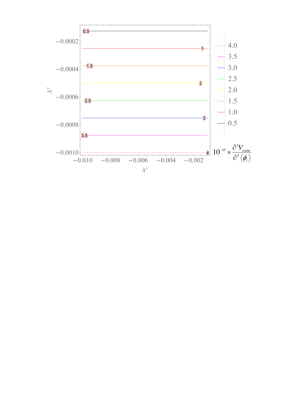
the quantities ∂2Vscalar∂⟨Φ⟩2​(Φ=H,ϕl,ϕν,η,ϕs,ηs)\frac{\partial^{2}V_{\mathrm{scalar}}}{\partial\langle\Phi\rangle^{2}}\,(\Phi=H,\phi_{l},\phi_{\nu},\eta,\phi_{s},\eta_{s}) depend on two parameters λx\lambda^{x} and λy\lambda^{y} with λx∈(−10−2,−10−3)\lambda^{x}\in(-10^{-2},-10^{-3}) and λy∈(−10−3,−10−4)\lambda^{y}\in(-10^{-3},-10^{-4}). Fig.1 implies that99 9 As an example, in the case of λx=−10−3\lambda^{x}=-10^{-3} and λy=−10−4\lambda^{y}=-10^{-4} we get ∂2Vscalar∂⟨H⟩2∼1043,∂2Vscalar∂⟨ϕl⟩2∼∂2Vscalar∂⟨ϕs⟩2\frac{\partial^{2}V_{\mathrm{scalar}}}{\partial\langle H\rangle^{2}}\sim 10^{43},\hskip 5.69046pt\frac{\partial^{2}V_{\mathrm{scalar}}}{\partial\langle\phi_{l}\rangle^{2}}\sim\frac{\partial^{2}V_{\mathrm{scalar}}}{\partial\langle\phi_{s}\rangle^{2}} ∼1034\sim 10^{34}, ∂2Vscalar∂⟨ϕν⟩2∼1053\frac{\partial^{2}V_{\mathrm{scalar}}}{\partial\langle\phi_{\nu}\rangle^{2}}\sim 10^{53} and ∂2Vscalar∂⟨η⟩2∼∂2Vscalar∂⟨ηs⟩2∼1042\frac{\partial^{2}V_{\mathrm{scalar}}}{\partial\langle\eta\rangle^{2}}\sim\frac{\partial^{2}V_{\mathrm{scalar}}}{\partial\langle\eta_{s}\rangle^{2}}\sim 10^{42}., the inequalities in (17) and (18) are always satisfied by the solutions of Eqs. (11)–(15) as given in Appendix B. This proves that the VEV alignments in Eq. (5) is the natural solution of the minimum condition of VscalarV_{\mathrm{scalar}} as expected.

Refer to caption
Refer to caption
Refer to caption
Refer to caption
Refer to caption
Refer to caption
Figure 1: ∂2Vscalar∂⟨Φ⟩2​(Φ=H,ϕl,ϕν,η,ϕs,ηs)\frac{\partial^{2}V_{\mathrm{scalar}}}{\partial\langle\Phi\rangle^{2}}\,(\Phi=H,\phi_{l},\phi_{\nu},\eta,\phi_{s},\eta_{s}) versus λx\lambda^{x} and λy\lambda^{y} with λx∈(−10−2,−10−3)\lambda^{x}\in(-10^{-2},-10^{-3}) and λy∈(−10−3,−10−4)\lambda^{y}\in(-10^{-3},-10^{-4}).

IV 3+1 active - sterile neutrino mixing

With the help of (5) and the Clebsch-Gordan coefficients of A4A_{4} group ishi, from Eq. (1) we get the charged lepton masses and the corresponding mixing matrices:

me\displaystyle m_{e} =\displaystyle= 2​3​x1​c​l​vH​(vlΛ)2,mμ=3​x2​c​l​vH​vlΛ,mτ=3​vH​x3​c​l​vlΛ,\displaystyle 2\sqrt{3}x_{1cl}v_{H}\left(\frac{v_{l}}{\Lambda}\right)^{2},\hskip 5.69046ptm_{\mu}=\sqrt{3}x_{2cl}v_{H}\frac{v_{l}}{\Lambda},\hskip 5.69046ptm_{\tau}=\sqrt{3}v_{H}x_{3cl}\frac{v_{l}}{\Lambda}, (23)
UL+\displaystyle U^{+}_{L} =\displaystyle= 13​(1   1   11ω2ω1ωω2),UR=1,ω=ei​2​π/3.\displaystyle\frac{1}{\sqrt{3}}\left(\begin{array}[]{ccc}1&\,\,\,1&\,\,\,1\\ 1&\,\,\,\omega^{2}&\,\,\,\omega\\ 1&\,\,\,\omega&\,\,\,\omega^{2}\\ \end{array}\right),\hskip 5.69046ptU_{R}=1,\hskip 5.69046pt\omega=e^{i2\pi/3}.

The Eq. (23) tells us that mem_{e} is suppressed by a factor of vH​(vlΛ)2∼10−4​GeVv_{H}\left(\frac{v_{l}}{\Lambda}\right)^{2}\sim 10^{-4}\,\mathrm{GeV} compared to mμm_{\mu} and mτm_{\tau} of the order of vH​vlΛ∼10−1​GeV\frac{v_{H}v_{l}}{\Lambda}\sim 10^{-1}\,\mathrm{GeV}. Thus, the considered model naturally explain the charged-lepton mass hierarchy.

By comparing me,μ,τm_{e,\mu,\tau} in (23) with the data given in Ref. PDG2020, me≃0.511​MeV,mμ≃105.66​MeVm_{e}\simeq 0.511\,\mathrm{MeV},m_{\mu}\simeq 105.66\,\mathrm{MeV} and mτ≃1776.86​MeVm_{\tau}\simeq 1776.86\,\mathrm{MeV}, along with the help of Eqs. (6)-(8), we obtain

x1​c​l=0.848,x2​c​l=0.351,x3​c​l=5.90.\displaystyle x_{1cl}=0.848,\hskip 5.69046ptx_{2cl}=0.351,\hskip 5.69046ptx_{3cl}=5.90. (28)

Coming back to the neutrino sector. Using the Clebsch-Gordan coefficient property of A4A_{4} group ishi, from Eq. (1), the Lagrangian for the neutrino sector becomes

−ℒν\displaystyle-\mathcal{L}_{\nu} =\displaystyle= x1​ν​(ψ¯1​L​ν1​R+ψ¯2​L​ν2​R+ψ¯3​L​ν3​R)​H~\displaystyle x_{1\nu}\left(\bar{\psi}_{1L}\nu_{1R}+\bar{\psi}_{2L}\nu_{2R}+\bar{\psi}_{3L}\nu_{3R}\right)\widetilde{H} (29)
+\displaystyle+ x2​νΛ​[(ψ¯2​L​ν3​R+ψ¯3​L​ν2​R)​H~​ϕ1​ν+(ψ¯3​L​ν1​R+ψ¯1​L​ν3​R)​H~​ϕ2​ν+(ψ¯1​L​ν2​R+ψ¯2​L​ν1​R)​H~​ϕ3​ν]\displaystyle\frac{x_{2\nu}}{\Lambda}\left[(\bar{\psi}_{2L}\nu_{3R}+\bar{\psi}_{3L}\nu_{2R})\widetilde{H}\phi_{1\nu}+(\bar{\psi}_{3L}\nu_{1R}+\bar{\psi}_{1L}\nu_{3R})\widetilde{H}\phi_{2\nu}+(\bar{\psi}_{1L}\nu_{2R}+\bar{\psi}_{2L}\nu_{1R})\widetilde{H}\phi_{3\nu}\right]
+\displaystyle+ x3​νΛ​[(ψ¯2​L​ν3​R−ψ¯3​L​ν2​R)​H~​ϕ1​ν+(ψ¯3​L​ν1​R−ψ¯1​L​ν3​R)​H~​ϕ2​ν+(ψ¯1​L​ν2​R−ψ¯2​L​ν1​R)​H~​ϕ3​ν]\displaystyle\frac{x_{3\nu}}{\Lambda}\left[(\bar{\psi}_{2L}\nu_{3R}-\bar{\psi}_{3L}\nu_{2R})\widetilde{H}\phi_{1\nu}+(\bar{\psi}_{3L}\nu_{1R}-\bar{\psi}_{1L}\nu_{3R})\widetilde{H}\phi_{2\nu}+(\bar{\psi}_{1L}\nu_{2R}-\bar{\psi}_{2L}\nu_{1R})\widetilde{H}\phi_{3\nu}\right]
+\displaystyle+ yν2​(ν¯1​Rc​ν1​R+ν¯2​Rc​ν2​R+ν¯2​Rc​ν3​R)​η+ysΛ​(ν¯sc​ν1​R​ηs​ϕ1​s+ν¯sc​ν2​R​ηs​ϕ2​s+ν¯sc​ν3​R​ηs​ϕ3​s)\displaystyle\frac{y_{\nu}}{2}\left(\bar{\nu}^{c}_{1R}\nu_{1R}+\bar{\nu}^{c}_{2R}\nu_{2R}+\bar{\nu}^{c}_{2R}\nu_{3R}\right)\eta+\frac{y_{s}}{\Lambda}\left(\bar{\nu}^{c}_{s}\nu_{1R}\eta_{{\color[rgb]{0,0,1}s}}\phi_{1s}+\bar{\nu}^{c}_{s}\nu_{2R}\eta_{{\color[rgb]{0,0,1}s}}\phi_{2s}+\bar{\nu}^{c}_{s}\nu_{3R}\eta_{{\color[rgb]{0,0,1}s}}\phi_{3s}\right)
+\displaystyle+ H.c.\displaystyle\mathrm{H.c}.

After symmetry breaking, we find the 7×77\times 7 neutrino mass matrix in the basis (νL,νRc,Sc)(\nu_{L},\nu^{c}_{R},S^{c}) as follows

Mν7×7=(0MD0MDTMRMST0MS0),\displaystyle M_{\nu}^{7\times 7}=\begin{pmatrix}0&M_{D}&0\\ M^{T}_{D}&M_{R}&M^{T}_{S}\\ 0&M_{S}&0\end{pmatrix}, (30)

where MD,MRM_{D},M_{R} and MSM_{S} take the form:

MD\displaystyle M_{D} =\displaystyle= vH​(x1​ν0vνΛ​(x2​ν−x3​ν)0x1​ν0vνΛ​(x2​ν+x3​ν)0x1​ν),\displaystyle v_{H}\left(\begin{array}[]{ccc}x_{1\nu}&0&\frac{v_{\nu}}{\Lambda}\left(x_{2\nu}-x_{3\nu}\right)\\ 0&x_{1\nu}&0\\ \frac{v_{\nu}}{\Lambda}\left(x_{2\nu}+x_{3\nu}\right)&0&x_{1\nu}\\ \end{array}\right),
MR\displaystyle M_{R} =\displaystyle= yν​vη​𝐈,Ms=ysΛ​vηs​vs​(101).\displaystyle y_{\nu}v_{\eta}\mathbf{I},\hskip 5.69046pt\hskip 5.69046ptM_{s}=\frac{y_{s}}{\Lambda}v_{\eta_{\color[rgb]{0,0,1}s}}v_{s}(1\hskip 9.95863pt0\hskip 9.95863pt1). (35)

In the case where MR≫MS>MDM_{R}\gg M_{S}>M_{D}, the effective 4×44\times 4 light neutrino mass matrix in the basis (νL,Sc)(\nu_{L},S^{c}) is constructed by the following expression Barry2011; Zhang2012; Das2019ea; Krishnan2020:

Mν=−(MD​MR−1​MDTMD​MR−1​MSTMS​(MR−1)T​MDTMS​MR−1​MST).M_{\nu}=-\left(\begin{array}[]{cc}M_{D}M^{-1}_{R}M^{T}_{D}&M_{D}M^{-1}_{R}M^{T}_{S}\\ M_{S}(M^{-1}_{R})^{T}M^{T}_{D}&M_{S}M^{-1}_{R}M^{T}_{S}\end{array}\right). (36)

The expression (35) shows that, there are five complex parameters thus has ten real parameters in the neutrino sector. Considering the case of real VEV for the singlet scalars ϕν,ϕs\phi_{\nu},\,\phi_{s} and η\eta, the phase redefinition of the leptonic fields ψL,νR\psi_{L},\nu_{R} and νs\nu_{s} allows to rotate away the phase of four neutrino Yukawa couplings x2​ν,x3​ν,yνx_{2\nu},x_{3\nu},y_{\nu} and ysy_{s}, reducing to six physical parameters. On the other hand, one parameter is absorbed by defining the hermitian matrix. Thus, in the neutrino sector, there are five real parameters, including α1=arg⁡(x1​ν)\alpha_{1}=\mathrm{arg}(x_{1\nu}), k2,3,m0k_{2,3},m_{0} and msm_{s} which are defined are defined as follows:

k2=vν​x2​νΛ​|x1​ν|,k3=vν​x3​νΛ​|x1​ν|,m0=vH2​|x1​ν|2vη​yν,ms=2​vηs2​vs2​ys2vη​Λ2​yν.\displaystyle k_{2}=\frac{v_{\nu}x_{2\nu}}{\Lambda|x_{1\nu}|},\hskip 5.69046ptk_{3}=\frac{v_{\nu}x_{3\nu}}{\Lambda|x_{1\nu}|},\hskip 5.69046ptm_{0}=\frac{v^{2}_{H}|x_{1\nu}|^{2}}{v_{\eta}y_{\nu}},\hskip 5.69046ptm_{s}=\frac{2v^{2}_{\eta_{s}}v^{2}_{s}y_{s}^{2}}{v_{\eta}\Lambda^{2}y_{\nu}}. (37)

Combining Eqs.(35) and (36) yields:

Mν4×4=−(m0​(e2​i​α1+(k2−k3)202​k2​ei​α10e2​i​α102​k2​ei​α10e2​i​α1+(k2+k3)2)m0​ms2​(ei​α1+(k2−k3)0ei​α1+(k2+k3))m0​ms2​(ei​α1+(k2−k3)0ei​α1+(k2+k3))ms),\displaystyle M^{4\times 4}_{\nu}=-\left(\begin{array}[]{cccc}\hskip-2.84544ptm_{0}\left(\begin{array}[]{ccc}e^{2i\alpha_{1}}+(k_{2}-k_{3})^{2}&0&2k_{2}e^{i\alpha_{1}}\\ 0&e^{2i\alpha_{1}}&0\\ 2k_{2}e^{i\alpha_{1}}&0&\hskip 5.69046pte^{2i\alpha_{1}}+(k_{2}+k_{3})^{2}\\ \end{array}\right)&\hskip-2.84544pt\sqrt{\frac{m_{0}m_{s}}{2}}\left(\begin{array}[]{c}e^{i\alpha_{1}}+(k_{2}-k_{3})\\ 0\\ e^{i\alpha_{1}}+(k_{2}+k_{3})\\ \end{array}\right)\\ \hskip-21.33955pt\sqrt{\frac{m_{0}m_{s}}{2}}\left(\begin{array}[]{ccc}e^{i\alpha_{1}}+(k_{2}-k_{3})&0&\hskip 5.69046pte^{i\alpha_{1}}+(k_{2}+k_{3})\\ \end{array}\right)&\quad\quad\quad\hskip 5.69046ptm_{s}\\ \end{array}\right),
(48)

where α1=arg⁡(x1​ν)\alpha_{1}=\mathrm{arg}(x_{1\nu}), and k2,3,m0k_{2,3},m_{0} and msm_{s} are defined in Eq. (37).

Suppose that MD<MsM_{D}<M_{s}, we can therefore apply the type-I seesaw mechanism on Eq.(36) to obtain the active neutrino mass matrix as Barry2011; Zhang2012; Das2019ea; Krishnan2020

Mν\displaystyle M_{\nu} =\displaystyle= MD​MR−1​MsT​(Ms​MR−1​MsT)−1​Ms​MR−1​MDT−MD​MR−1​MDT\displaystyle M_{D}M_{R}^{-1}M_{s}^{T}(M_{s}M_{R}^{-1}M_{s}^{T})^{-1}M_{s}M_{R}^{-1}M_{D}^{T}-M_{D}M_{R}^{-1}M_{D}^{T}
=\displaystyle= −m02​((ei​α1−(k2−k3))20k32−(ei​α1−k2)202​e2​i​α10k32−(ei​α1−k2)20(ei​α1−(k2+k3))2).\displaystyle-\frac{m_{0}}{2}\left(\begin{array}[]{ccc}\left(e^{i\alpha_{1}}-(k_{2}-k_{3})\right)^{2}&0&k_{3}^{2}-(e^{i\alpha_{1}}-k_{2})^{2}\\ 0&2e^{2i\alpha_{1}}&0\\ k_{3}^{2}-(e^{i\alpha_{1}}-k_{2})^{2}&0&\left(e^{i\alpha_{1}}-(k_{2}+k_{3})\right)^{2}\\ \end{array}\right).

Since k2,3k_{2,3} and m0m_{0} are real, MνM_{\nu} is complex. To diagonalise the matrix MνM_{\nu}, let us define a Hermitian matrix 𝐦ν2\mathbf{m}^{2}_{\nu}, given by

𝐦ν2=\displaystyle\mathbf{m}^{2}_{\nu}= Mν​Mν†=m022​(A1+A20−B1+i​B​2020−B1−i​B20A1−A2),\displaystyle M_{\nu}M^{\dagger}_{\nu}=\frac{m^{2}_{0}}{2}\left(\begin{array}[]{ccc}A_{1}+A_{2}&0&-B_{1}+iB2\\ 0&2&0\\ -B_{1}-iB_{2}&0&A_{1}-A_{2}\\ \end{array}\right),

where

A1=(1+k22+k32−2k2cosα1)2,\displaystyle A_{1}=\left(1+k_{2}^{2}+k_{3}^{2}-2k_{2}\cos\alpha_{1}\right)^{2},
A2=2k3(cosα1−k2)(1+k22+k32−2k2cosα1),\displaystyle A_{2}=2k_{3}(\cos\alpha_{1}-k_{2})(1+k_{2}^{2}+k_{3}^{2}-2k_{2}\cos\alpha_{1}),
B1=(1+k22−k32−2k2cosα1)(1+k22+k32−2k2cosα1),\displaystyle B_{1}=(1+k_{2}^{2}-k_{3}^{2}-2k_{2}\cos\alpha_{1})(1+k_{2}^{2}+k_{3}^{2}-2k_{2}\cos\alpha_{1}),
B2=2k3(1+k22+k32−2k2cosα1)sinα1.\displaystyle B_{2}=2k_{3}(1+k_{2}^{2}+k_{3}^{2}-2k_{2}\cos\alpha_{1})\sin\alpha_{1}. (57)

The matrix 𝐦ν2\mathbf{m}^{2}_{\nu} in Eq. (IV) is diagonalized by UνU_{\nu} satisfying

Uν+​𝐦ν2​Uν={(0000m02000k02​m02),Uν=(1x1+i​x20−1y1+i​y20101x001y0)​for NH,(k02​m02000m020000),Uν=(−1y1+i​y201x1+i​x20101y001x0)​for IH,U_{\nu}^{+}\mathbf{m}^{2}_{\nu}U_{\nu}=\left\{\begin{array}[]{l}\left(\begin{array}[]{ccc}0&0&0\\ 0&m^{2}_{0}&0\\ 0&0&k^{2}_{0}m^{2}_{0}\\ \end{array}\right),\hskip 2.84544ptU_{\nu}=\left(\begin{array}[]{ccc}\frac{1}{x_{1}+ix_{2}}&0&\hskip 5.69046pt-\frac{1}{y_{1}+iy_{2}}\\ 0&1&0\\ \frac{1}{x_{0}}&0&\frac{1}{y_{0}}\\ \end{array}\right)\hskip 5.69046pt\mbox{for NH,}\\ \left(\begin{array}[]{ccc}k^{2}_{0}m^{2}_{0}&0&0\\ 0&m^{2}_{0}&0\\ 0&0&0\\ \end{array}\right),\hskip 2.84544ptU_{\nu}=\left(\begin{array}[]{ccc}-\frac{1}{y_{1}+iy_{2}}&0&\hskip 5.69046pt\frac{1}{x_{1}+ix_{2}}\\ 0&1&0\\ \frac{1}{y_{0}}&0&\frac{1}{x_{0}}\\ \end{array}\right)\hskip 5.69046pt\mbox{for IH,}\end{array}\right. (58)

thus the light neutrino masses are

{m21=0,m22=m20,m23=m20k20for NH,m21=m20k20,m22=m20,m23=0for IH,\displaystyle\left\{\begin{array}[]{l}m^{2}_{1}=0,\hskip 20.62842ptm^{2}_{2}=m^{2}_{0},\hskip 2.84544ptm^{2}_{3}=m^{2}_{0}k^{2}_{0}\hskip 5.69046pt\mbox{for NH},\\ m^{2}_{1}=m^{2}_{0}k^{2}_{0},\hskip 1.42271ptm^{2}_{2}=m^{2}_{0},\hskip 2.84544ptm^{2}_{3}=0\hskip 22.76228pt\,\mbox{for IH},\end{array}\right.

where

k0=1+k22+k32−2k2cosα1,\displaystyle k_{0}=1+k_{2}^{2}+k_{3}^{2}-2k_{2}\cos\alpha_{1}, (62)
x0=2​k0k0+2​k3​(cos⁡α1−k2),y0=2​k0k0+2​k3​(k2−cos⁡α1),\displaystyle x_{0}=\sqrt{\frac{2k_{0}}{k_{0}+2k_{3}(\cos\alpha_{1}-k_{2})}},\hskip 1.42271pty_{0}=\sqrt{\frac{2k_{0}}{k_{0}+2k_{3}(k_{2}-\cos\alpha_{1})}}, (63)
x1=(k0−2​k32)​x0k0+2​k3​(k2−cos⁡α1),y1=(k0−2​k32)​y0k0+2​k3​(cos⁡α1−k2),\displaystyle x_{1}=\frac{(k_{0}-2k^{2}_{3})x_{0}}{k_{0}+2k_{3}(k_{2}-\cos\alpha_{1})},\hskip 12.80365pty_{1}=\frac{(k_{0}-2k^{2}_{3})y_{0}}{k_{0}+2k_{3}(\cos\alpha_{1}-k_{2})}, (64)
x2=2k3x0sinα1k0+2​k3​(k2−cos⁡α1),y2=2k3y0sinα1k0+2​k3​(cos⁡α1−k2).\displaystyle x_{2}=\frac{2k_{3}x_{0}\sin\alpha_{1}}{k_{0}+2k_{3}(k_{2}-\cos\alpha_{1})},\hskip 12.80365pty_{2}=\frac{2k_{3}y_{0}\sin\alpha_{1}}{k_{0}+2k_{3}(\cos\alpha_{1}-k_{2})}. (65)

The corresponding leptonic mixing matrix is

Ul​e​p=UL†​Uν={13​(1x0+1x1+i​x211y0−1y1+i​y2ωx0+1x1+i​x2ω2ωy0−1y1+i​y2ω2x0+1x1+i​x2ωω2y0−1y1+i​y2)​for   NH,13​(1y0−1y1+i​y211x0+1x1+i​x2ωy0−1y1+i​y2ω2ωx0+1x1+i​x2ω2y0−1y1+i​y2ωω2x0+1x1+i​x2)​for   IH,U_{lep}=U_{L}^{{\dagger}}U_{\nu}=\left\{\begin{array}[]{l}\frac{1}{\sqrt{3}}\left(\begin{array}[]{ccc}\frac{1}{x_{0}}+\frac{1}{x_{1}+ix_{2}}&1&\frac{1}{y_{0}}-\frac{1}{y_{1}+iy_{2}}\\ \frac{\omega}{x_{0}}+\frac{1}{x_{1}+ix_{2}}&\omega^{2}&\hskip 5.69046pt\frac{\omega}{y_{0}}-\frac{1}{y_{1}+iy_{2}}\\ \frac{\omega^{2}}{x_{0}}+\frac{1}{x_{1}+ix_{2}}&\omega&\hskip 5.69046pt\frac{\omega^{2}}{y_{0}}-\frac{1}{y_{1}+iy_{2}}\\ \end{array}\right)\hskip 5.69046pt\mbox{for \, NH},\\ \frac{1}{\sqrt{3}}\left(\begin{array}[]{ccc}\frac{1}{y_{0}}-\frac{1}{y_{1}+iy_{2}}&1&\frac{1}{x_{0}}+\frac{1}{x_{1}+ix_{2}}\\ \frac{\omega}{y_{0}}-\frac{1}{y_{1}+iy_{2}}&\omega^{2}&\hskip 5.69046pt\frac{\omega}{x_{0}}+\frac{1}{x_{1}+ix_{2}}\\ \frac{\omega^{2}}{y_{0}}-\frac{1}{y_{1}+iy_{2}}&\omega&\hskip 5.69046pt\frac{\omega^{2}}{x_{0}}+\frac{1}{x_{1}+ix_{2}}\\ \end{array}\right)\hskip 5.69046pt\mbox{for \, IH},\end{array}\right. (66)

which being being the TM2\mathrm{TM}_{2} form. Eq. (IV) implies the neutrino mass ordering should be either (0,m0,m0​k0)(0,m_{0},m_{0}k_{0}) or (m0​k0,m0,0)(m_{0}k_{0},m_{0},0). It is very interesting to note that depending on the sign of cos⁡α1\cos\alpha_{1}, k0k_{0} can be greater or less than 1 so both NH (m1<m2m_{1}<m_{2}) and IH (m2<m1m_{2}<m_{1}) are consistent with the experimental data given that k2k_{2} and k3k_{3} are real parameters. Threrefore, our model predicts both NH and IH of the active neutrino masses which is in consistent with the data taken from Ref. Salas2020 and different from that of Ref. Krishnan2020.

The lepton mixing angles, in the three-neutrino scheme, is defined as PDG2020

s132=|Ue​3|2={23​k32k0​for   NH,23​(1−k32k0)​for   IH,\displaystyle s_{13}^{2}=\left|\mathrm{U}_{e3}\right|^{2}=\left\{\begin{array}[]{l}\frac{2}{3}\frac{k_{3}^{2}}{k_{0}}\hskip 8.5359pt\mbox{for \, NH},\\ \frac{2}{3}\left(1-\frac{k^{2}_{3}}{k_{0}}\right)\hskip 7.11317pt\,\mbox{for \, IH},\end{array}\right.
s122=|Ue​2|21−|Ue​3|2=13​c132​for   both  NH  and   IH,\displaystyle s_{12}^{2}=\frac{\left|\mathrm{U}_{e2}\right|^{2}}{1-\left|\mathrm{U}_{e3}\right|^{2}}=\frac{1}{3c^{2}_{13}}\hskip 7.11317pt\,\mbox{for \, both \,NH\, and \, IH}, (70)
s232=|Uμ​3|21−|Ue​3|2={12+3k3sinα13​k0−2​k32​for   NH,12−3k3sinα1k0+2​k32​for   IH,\displaystyle s_{23}^{2}=\frac{\left|\mathrm{U}_{\mu 3}\right|^{2}}{1-\left|\mathrm{U}_{e3}\right|^{2}}=\left\{\begin{array}[]{l}\frac{1}{2}+\frac{\sqrt{3}k_{3}\sin\alpha_{1}}{3k_{0}-2k_{3}^{2}}\hskip 8.5359pt\mbox{for \, NH},\\ \frac{1}{2}-\frac{\sqrt{3}k_{3}\sin\alpha_{1}}{k_{0}+2k_{3}^{2}}\hskip 7.11317pt\,\mbox{for \, IH},\end{array}\right.

where θi​j\theta_{ij} are neutrino mixing angles and t12=s12/c12t_{12}=s_{12}/c_{12}, t23=s23/c23t_{23}=s_{23}/c_{23}, ci​j=cos⁡θi​jc_{ij}=\cos\theta_{ij}, si​j=sin⁡θi​js_{ij}=\sin\theta_{ij}.

The Jarlskog invariant, determined from Eq. (66), takes the form Jarlskog1; Jarlskog2; Jarlskog3; PDG2020

JC​P\displaystyle J_{CP} =\displaystyle= Im⁡(U12​U23​U13∗​U22∗)={k3​(cos⁡α1−k2)3​3​k0​for   NH,k3​(k2−cos⁡α1)3​3​k0​for   IH.\displaystyle\mathrm{Im}(U_{12}U_{23}U^{*}_{13}U^{*}_{22})=\left\{\begin{array}[]{l}\frac{k_{3}(\cos\alpha_{1}-k_{2})}{3\sqrt{3}k_{0}}\hskip 8.5359pt\mbox{for \, NH},\\ \frac{k_{3}(k_{2}-\cos\alpha_{1})}{3\sqrt{3}k_{0}}\hskip 7.11317pt\,\mbox{for \, IH}.\end{array}\right.

From Eqs. (58) and (IV)-(IV), we can express m0,k0,k2,3m_{0},k_{0},k_{2,3} and sin⁡δC​P\sin\delta_{CP} in terms of four observables Δ​m212,Δ​m312\Delta m^{2}_{21},\Delta m^{2}_{31}, s232s^{2}_{23} and s132s^{2}_{13} and α1\alpha_{1} as follows:

m02={Δ​m212for NH,Δ​m212−Δ​m312​for  IH,\displaystyle m^{2}_{0}=\left\{\begin{array}[]{l}\Delta m^{2}_{21}\hskip 44.813pt\mbox{for NH},\\ \Delta m^{2}_{21}-\Delta m^{2}_{31}\hskip 2.84544pt\,\mbox{for\, IH},\end{array}\right.
k02={Δ​m312m02for   NH,−Δ​m312m02​for   IH,\displaystyle k^{2}_{0}=\left\{\begin{array}[]{l}\frac{\Delta m^{2}_{31}}{m^{2}_{0}}\hskip 11.38092pt\mbox{for \, NH},\\ \frac{-\Delta m^{2}_{31}}{m^{2}_{0}}\hskip 2.84544pt\,\mbox{for \, IH},\end{array}\right.
k2=cos⁡α1∓k0−k32−sin2⁡α1​for both NH and IH,\displaystyle k_{2}=\cos\alpha_{1}\mp\sqrt{k_{0}-k_{3}^{2}-\sin^{2}\alpha_{1}}\hskip 7.11317pt\mbox{for\ both\ NH\ and IH,} (83)
k32={32​k0​s132for   NH,k02​(2−3​s132)​for   IH,\displaystyle k^{2}_{3}=\left\{\begin{array}[]{l}\frac{3}{2}k_{0}s^{2}_{13}\hskip 34.14322pt\mbox{for \, NH},\\ \frac{k_{0}}{2}\left(2-3s^{2}_{13}\right)\hskip 1.42271pt\,\mbox{for \, IH},\end{array}\right.
sin⁡δC​P=3​JC​Ps13​s23​c23​2−3​s132​for both NH and IH,\displaystyle\sin\delta_{CP}=\frac{3J_{CP}}{s_{13}s_{23}c_{23}\sqrt{2-3s^{2}_{13}}}\hskip 7.11317pt\mbox{for\ both\ NH\ and IH,} (87)

with JC​PJ_{CP} is determined in Eq. (IV).

Using the approximation MD<MsM_{D}<M_{s}, we obtain the mass of the 4th4^{\text{th}} mass eigenstate Barry2011; Zhang2012; Das2019ea; Krishnan2020,

m4=−Ms​MR−1​MsT=ms,\displaystyle m_{4}=-M_{s}M_{R}^{-1}M_{s}^{T}=m_{s}, (88)

with msm_{s} is defined in Eq. (37). Combining Eqs. (IV) and (88) yields:

ms=m4={Δ​m412for NH,Δ​m412+m02​k02​for IH.\displaystyle m_{s}=m_{4}=\left\{\begin{array}[]{l}\sqrt{\Delta m^{2}_{41}}\hskip 11.38092pt\mbox{for NH},\\ \sqrt{\Delta m^{2}_{41}+m^{2}_{0}k^{2}_{0}}\hskip 2.84544pt\,\mbox{for IH}.\end{array}\right.

The 4×44\times 4 light neutrino mixing matrix is given by Barry2011; Zhang2012; Das2019ea; Krishnan2020:

U=UL†​Uν=(UL†​(1−12​R​R†)​UνUL†​R−R†​Uν1−12​R†​R),\displaystyle U=U^{\dagger}_{L}U_{\nu}=\left(\begin{array}[]{cc}U^{\dagger}_{L}(1-\frac{1}{2}RR^{\dagger})U_{\nu}&U^{\dagger}_{L}R\\ -R^{\dagger}U_{\nu}&1-\frac{1}{2}R^{\dagger}R\end{array}\right),

where the three-component column vector RR is given by Barry2011; Zhang2012; Das2019ea; Krishnan2020

R=MD​MR−1​MsT​(Ms​MR−1​MsT)−1=m02​ms​(ei​α1+(k2−k3)0ei​α1+(k2+k3)).\displaystyle R=M_{D}M_{R}^{-1}M_{s}^{T}(M_{s}M_{R}^{-1}M_{s}^{T})^{-1}=\sqrt{\frac{m_{0}}{2m_{s}}}\left(\begin{array}[]{c}e^{i\alpha_{1}}+(k_{2}-k_{3})\\ 0\\ e^{i\alpha_{1}}+(k_{2}+k_{3})\\ \end{array}\right).

Combining Eqs. (IV) and (IV), the strength of the active-sterile mixing is given by

UL†​R\displaystyle U^{\dagger}_{L}R =\displaystyle= 16​m0ms​(2​(ei​α1+k2)12​[(1−i​3)​(k2+ei​α1)−(3+i​3)​k3]12​[(1+i​3)​(k2+ei​α1)−(3−i​3)​k3])≡(Ue​4Uμ​4Uτ​4),\displaystyle\frac{1}{\sqrt{6}}\sqrt{\frac{m_{0}}{m_{s}}}\left(\begin{array}[]{c}2(e^{i\alpha_{1}}+k_{2})\\ \frac{1}{2}\left[\left(1-i\sqrt{3}\right)\left(k_{2}+e^{i\alpha_{1}}\right)-\left(3+i\sqrt{3}\right)k_{3}\right]\\ \frac{1}{2}\left[\left(1+i\sqrt{3}\right)\left(k_{2}+e^{i\alpha_{1}}\right)-\left(3-i\sqrt{3}\right)k_{3}\right]\\ \end{array}\right)\equiv\left(\begin{array}[]{c}U_{e4}\\ U_{\mu 4}\\ U_{\tau 4}\\ \end{array}\right),

which leads to

|U14|2=23m0ms(1+k22+2k2cosα1),\displaystyle|U_{14}|^{2}=\frac{2}{3}\frac{m_{0}}{m_{s}}\left(1+k_{2}^{2}+2k_{2}\cos\alpha_{1}\right), (106)
|U24|2=16m0ms(1+k22+3k32+2k2cosα1−23k3sinα1),\displaystyle|U_{24}|^{2}=\frac{1}{6}\frac{m_{0}}{m_{s}}\left(1+k_{2}^{2}+3k_{3}^{2}+2k_{2}\cos\alpha_{1}-2\sqrt{3}k_{3}\sin\alpha_{1}\right), (107)
|U34|2=16m0ms(1+k22+3k32+2k2cosα1+23k3sinα1).\displaystyle|U_{34}|^{2}=\frac{1}{6}\frac{m_{0}}{m_{s}}\left(1+k_{2}^{2}+3k_{3}^{2}+2k_{2}\cos\alpha_{1}+2\sqrt{3}k_{3}\sin\alpha_{1}\right). (108)

The effective neutrino masses betdecay1; betdecay2; betdecay3, determined from Eqs. (IV), (66), (88) and (IV), possess the following forms1010 10 Eqs. (109) and (110) are satisfied for both NH and IH.:

⟨me​e⟩=|∑i=14Ue​i2​mi|=m03​Γek0+2k3(k2−2cosα1),\displaystyle\langle m_{ee}\rangle=\left|\sum^{4}_{i=1}U_{ei}^{2}m_{i}\right|=\frac{m_{0}}{3}\sqrt{\frac{\Gamma_{\mathrm{e}}}{k_{0}+2k_{3}(k_{2}-2\cos\alpha_{1})}}, (109)
mβ=∑i=14|Ue​i|2​mi2=m03​1+2k0k32+2​msm0(1+k22+2k2cosα1),\displaystyle m_{\beta}=\sqrt{\sum^{4}_{i=1}\left|U_{ei}\right|^{2}m_{i}^{2}}=\frac{m_{0}}{\sqrt{3}}\sqrt{1+2k_{0}k_{3}^{2}+\frac{2m_{s}}{m_{0}}\left(1+k_{2}^{2}+2k_{2}\cos\alpha_{1}\right)}, (110)
⟨me​e(3​ν)⟩=|∑i=13Ue​i2​mi|=m03​Γe(3)k0+2k3(k2−2cosα1),\displaystyle\langle m^{(3\nu)}_{ee}\rangle=\left|\sum^{3}_{i=1}U_{ei}^{2}m_{i}\right|=\frac{m_{0}}{3}\sqrt{\frac{\Gamma^{(3)}_{\mathrm{e}}}{k_{0}+2k_{3}(k_{2}-2\cos\alpha_{1})}}, (111)
mβ(3​ν)=∑i=13|Ue​i|2​mi2=m03​1+2​k0​k32,\displaystyle m^{(3\nu)}_{\beta}=\sqrt{\sum^{3}_{i=1}\left|U_{ei}\right|^{2}m_{i}^{2}}=\frac{m_{0}}{\sqrt{3}}\sqrt{1+2k_{0}k_{3}^{2}}, (112)

with

Γe\displaystyle\Gamma_{\mathrm{e}} =\displaystyle= 5+(1+8​k22+4​k24)​k22+2​[4​k22​(3+k22)−7]​k2​k3+[12​(2+k22)​k22+5]​k32\displaystyle 5+(1+8k_{2}^{2}+4k_{2}^{4})k_{2}^{2}+2[4k_{2}^{2}(3+k_{2}^{2})-7]k_{2}k_{3}+[12(2+k_{2}^{2})k_{2}^{2}+5]k_{3}^{2} (113)
+\displaystyle+ 8(2k22+1)k2k33+4(3k22+2)k34+4(2k2+k3)k35+2[4(k23+3k22k3+2k33)k22\displaystyle 8(2k_{2}^{2}+1)k_{2}k_{3}^{3}+4(3k_{2}^{2}+2)k_{3}^{4}+4(2k_{2}+k_{3})k_{3}^{5}+2\left[4(k_{2}^{3}+3k_{2}^{2}k_{3}+2k_{3}^{3})k_{2}^{2}\right.
−\displaystyle- 7k3+(8k32−4)k23+(5+8k32+4k34)k2−4(1+k32)k33]cosα1\displaystyle\left.7k_{3}+(8k_{3}^{2}-4)k_{2}^{3}+(5+8k_{3}^{2}+4k_{3}^{4})k_{2}-4(1+k_{3}^{2})k_{3}^{3}\right]\cos\alpha_{1}
−\displaystyle- 4​[(2​k24−1)+(3+2​k32)​k22+4​(1+k32)​k2​k3−2​(1+k32)​k32]​cos⁡2​α1\displaystyle 4\left[(2k_{2}^{4}-1)+(3+2k_{3}^{2})k_{2}^{2}+4(1+k_{3}^{2})k_{2}k_{3}-2(1+k_{3}^{2})k_{3}^{2}\right]\cos 2\alpha_{1}
−\displaystyle- 4​[(1+2​k22)​(k2+k3)+4​k33]​cos⁡3​α1+8​k32​cos⁡4​α1,\displaystyle 4\left[(1+2k_{2}^{2})(k_{2}+k_{3})+4k_{3}^{3}\right]\cos 3\alpha_{1}+8k_{3}^{2}\cos 4\alpha_{1},
Γe(3)\displaystyle\Gamma^{(3)}_{\mathrm{e}} =\displaystyle= 1+4k32(k32+cos2α1)+(1+2k32)2[(k2+k3)2−2(k2+k3)cosα1].\displaystyle 1+4k_{3}^{2}\left(k^{2}_{3}+\cos 2\alpha_{1}\right)+(1+2k_{3}^{2})^{2}\left[(k_{2}+k_{3})^{2}-2(k_{2}+k_{3})\cos\alpha_{1}\right]. (114)

Although the NH seems favored by some global analysisCapozzi2017; Salas2018; Esteban2019, however, it is the fact that the neutrino mass spectrum is currently unknown and it can be normal (m1<m2<m3m_{1}<m_{2}<m_{3}) or inverted (m3<m1<m2m_{3}<m_{1}<m_{2}) ordering depending on the sign of Δ​m312\Delta m^{2}_{31} Salas2020; Kelly2021. In the next section, we will show that our model can explain the stirile-active neutrino mas and mixing as well as the recent three neutrino oscillation data given in Table 1 in the minimal extended seesaw framework for both NH and IH.

V Numerical analysis

In this work, eleven independent experimentally measured quantities in the neutrino sector, including sin2⁡θ12\sin^{2}\theta_{12}, sin2⁡θ23\sin^{2}\theta_{23}, sin2⁡θ13\sin^{2}\theta_{13}, sin⁡δ\sin\delta, Δ​m212\Delta m^{2}_{21}, Δ​m312\Delta m^{2}_{31}, ⟨me​e⟩\langle m_{ee}\rangle, Δ​m412\Delta m^{2}_{41}, |U14|2|U_{14}|^{2}, |U24|2|U_{24}|^{2} and |U34|2|U_{34}|^{2}, can be expressed in terms of five model parameters including k2k_{2}, k3k_{3}, m0m_{0}, msm_{s} and α1\alpha_{1}. We calculate the model parameters using the experimental data and also make predictions. To calculate the allowed ranges of the model parameters k2k_{2}, k3k_{3}, m0,msm_{0},m_{s} and α1\alpha_{1} as well as predictive ranges for the experimental parameters sin2⁡θ12\sin^{2}\theta_{12}, sin⁡δ\sin\delta, ⟨me​e⟩\langle m_{ee}\rangle, |U14|2|U_{14}|^{2}, |U24|2|U_{24}|^{2} and |U34|2|U_{34}|^{2}, we utilize the observables Δ​m212\Delta m^{2}_{21}, Δ​m312,Δ​m412\Delta m^{2}_{31},\Delta m^{2}_{41}, sin2⁡θ13\sin^{2}\theta_{13} and sin2⁡θ23\sin^{2}\theta_{23} whose experimental values are shown in Table 1.

Firstly, using the 3​σ3\sigma experimental range of Δ​m212\Delta m^{2}_{21} and Δ​m312\Delta m^{2}_{31} taken from Tab. 1, we get the constraints

m02∈{(69.4,81.4)​meV2​for NH,(2439,2611)​meV2​for IH,\displaystyle m^{2}_{0}\in\left\{\begin{array}[]{l}(69.4,81.4)\,\mathrm{meV}^{2}\hskip 7.11317pt\mbox{for NH},\\ (2439,2611)\,\mathrm{meV}^{2}\hskip 7.11317pt\mbox{for IH},\end{array}\right.
k02∈{(30.34,37.90)​meV​for NH,(0.967,0.973)​meV​for IH,\displaystyle k^{2}_{0}\in\left\{\begin{array}[]{l}(30.34,37.90)\,\mathrm{meV}\hskip 7.11317pt\mbox{for NH},\\ (0.967,0.973)\,\mathrm{meV}\hskip 7.11317pt\mbox{for IH},\end{array}\right.

In 3​σ3\sigma range of s13s_{13} Salas2020, 2.000×10⁻²<s132<2.405×10−22.000\times 10^{-2}<s^{2}_{13}<2.405\times 10^{-2} for NH and 2.018×10⁻²<s132<2.424×10−22.018\times 10^{-2}<s^{2}_{13}<2.424\times 10^{-2} for IH; thus, Eq. (70) implies that

s122∈{(0.3401,0.3415)​for NH,(0.3402,0.3416)​for IH,\displaystyle s^{2}_{12}\in\left\{\begin{array}[]{l}(0.3401,0.3415)\hskip 7.11317pt\mbox{for NH},\\ (0.3402,0.3416)\hskip 7.11317pt\mbox{for IH},\end{array}\right.

i.e.,

θ12(∘)∈{(35.68,35.76)​for NH,(35.68,35.77)​for IH,\displaystyle\theta_{12}(^{\circ})\in\left\{\begin{array}[]{l}(35.68,35.76)\hskip 7.11317pt\mbox{for NH},\\ (35.68,35.77)\hskip 7.11317pt\mbox{for IH},\end{array}\right.

which all belong to 3​σ3\sigma range of s122s^{2}_{12} Salas2020 as given in Tab. 1.

Next, using the constraints of k0k_{0} in Eq. (V) and the 3​σ3\sigma range of reactor mixing angle s13s_{13}, i.e., s132∈(2.00, 2.405)​10−2s^{2}_{13}\in(2.00,\,2.405)10^{-2} for NH and s132∈(2.018, 2.424)​10−2s^{2}_{13}\in(2.018,\,2.424)10^{-2} for IH, from Eq. (IV), we can depict the dependence of k32k^{2}_{3} on k02k^{2}_{0} and s132s^{2}_{13} as shown in Fig. 2, which implies that

k32∈{(0.17, 0.22)​for NH,(0.948,0.956)​for IH.\displaystyle k^{2}_{3}\in\left\{\begin{array}[]{l}(0.17,\,0.22)\hskip 7.11317pt\mbox{for NH},\\ (0.948,0.956)\hskip 7.11317pt\mbox{for IH}.\end{array}\right.
Refer to caption
Refer to caption
Figure 2: The contour plot of k32k^{2}_{3} as a function of k02k^{2}_{0} and s132s^{2}_{13} with k02∈(30.34,37.9)k^{2}_{0}\in(30.34,37.9) and s132∈(2.00,2.405)​10−2s^{2}_{13}\in(2.00,2.405)10^{-2} for NH (left panel) while k02∈(0.967,0.973)k^{2}_{0}\in(0.967,0.973) and s132∈(2.018,2.424)​10−2s^{2}_{13}\in(2.018,2.424)10^{-2} for IH (right panel).

Equation (IV) shows that s232s^{2}_{23} depends on k0,k3k_{0},k_{3} and sin⁡α1\sin\alpha_{1}. At the best-fit values of Δ​m212\Delta m^{2}_{21} and Δ​m312\Delta m^{2}_{31}, we get

m02={75.0​meV2​for NH,2525.0​meV2​for IH,​k02={34.0​for NH,0.9703​for IH,\displaystyle m^{2}_{0}=\left\{\begin{array}[]{l}75.0\,\mathrm{meV}^{2}\hskip 7.11317pt\mbox{for NH},\\ 2525.0\,\mathrm{meV}^{2}\hskip 7.11317pt\mbox{for IH},\end{array}\right.\hskip 5.69046ptk^{2}_{0}=\left\{\begin{array}[]{l}34.0\hskip 7.11317pt\mbox{for NH},\\ 0.9703\hskip 7.11317pt\mbox{for IH},\end{array}\right.
{m1=0meV,m2=8.66meV,m3=50.50meVfor NH,m1=49.50meV,m2=50.25meV,m3=0meVfor IH,\displaystyle\left\{\begin{array}[]{l}m_{1}=0\,\mathrm{meV},\hskip 5.69046ptm_{2}=8.66\,\mathrm{meV},\hskip 5.69046ptm_{3}=50.50\,\mathrm{meV}\hskip 7.11317pt\mbox{for NH},\\ m_{1}=49.50\,\mathrm{meV},\hskip 5.69046ptm_{2}=50.25\,\mathrm{meV},\hskip 5.69046ptm_{3}=0\,\mathrm{meV}\hskip 7.11317pt\mbox{for IH},\end{array}\right.

and we find the ranges of sin⁡α1\sin\alpha_{1} that of s232s^{2}_{23} lies in 3​σ3\sigma range given in Table 1 as depicted in Fig. 3 which implies

s232∈{(0.46,0.54)​for NH,(0.44,0.60)​for IH.\displaystyle s^{2}_{23}\in\left\{\begin{array}[]{l}(0.46,0.54)\hskip 7.11317pt\mbox{for NH},\\ (0.44,0.60)\hskip 7.11317pt\mbox{for IH}.\end{array}\right.
Refer to caption
Refer to caption
Figure 3: s232s^{2}_{23} versus k32k^{2}_{3} and sin⁡α1\sin\alpha_{1} with k32∈(0.17,0.22)k^{2}_{3}\in(0.17,0.22) and sin⁡α1∈(−1, 1)\sin\alpha_{1}\in(-1,\,1) for NH (left panel) while k32∈(0.948,0.956)k^{2}_{3}\in(0.948,0.956) and sin⁡α1∈(−0.065, 0.045)\sin\alpha_{1}\in(-0.065,\,0.045) for IH (right panel).

Further, Eqs. (IV) and (83)-(87) impliy that, at the best-fit values of Δ​m212\Delta m^{2}_{21} and Δ​m312\Delta m^{2}_{31}, k2k_{2} and sin⁡δC​P\sin\delta_{CP} depend on two parameters θ13\theta_{13} and θ23\theta_{23} which are plotted in Figs. 4 and 5, respectively. These figures indicates that

k2∈{(2.00,3.40)​for NH,(0.68,0.80)​for IH,\displaystyle k_{2}\in\left\{\begin{array}[]{l}(2.00,3.40)\hskip 7.11317pt\mbox{for NH},\\ (0.68,0.80)\hskip 7.11317pt\mbox{for IH},\end{array}\right.
sin⁡δC​P∈{(−0.60,−0.20)​for NH,(−0.95,−0.60)​for IH,\displaystyle\sin\delta_{CP}\in\left\{\begin{array}[]{l}(-0.60,-0.20)\hskip 7.11317pt\mbox{for NH},\\ (-0.95,-0.60)\hskip 7.11317pt\mbox{for IH},\end{array}\right.
Refer to caption
Refer to caption
Figure 4: k2k_{2} versus s132s^{2}_{13} and s232s^{2}_{23} with s132∈(2.00,2.405)​ 10−2s^{2}_{13}\in(2.00,2.405)\,10^{-2} and s232∈(0.46,0.54)s^{2}_{23}\in(0.46,0.54) for NH (left panel) while s132∈(2.018,2.424)​ 10−2s^{2}_{13}\in(2.018,2.424)\,10^{-2} and s232∈(0.44,0.60)s^{2}_{23}\in(0.44,0.60) for IH (right panel).
Refer to caption
Refer to caption
Figure 5: sin⁡δC​P\sin\delta_{CP} versus s132s^{2}_{13} and s232s^{2}_{23} with s132∈(2.00,2.405)​ 10−2s^{2}_{13}\in(2.00,2.405)\,10^{-2} and s232∈(0.46,0.54)s^{2}_{23}\in(0.46,0.54) for NH (left panel) while s132∈(2.018,2.424)​ 10−2s^{2}_{13}\in(2.018,2.424)\,10^{-2} and s232∈(0.44,0.60)s^{2}_{23}\in(0.44,0.60) for IH (right panel).

At present, there are various experimental bounds on Δ​m412\Delta m^{2}_{41} Aguilar2001; Arevalo2013; Acero2008; Arevalo2010; Mention2011; An2014; Arevalo2018; Gariazzo17; Adamson2019; Adamson2020; Aartsen2020; Beheraa2019; BeheraPRD2020, for example, Δ​m412∈(0.01,1.0)​eV2\Delta m^{2}_{41}\in(0.01,1.0)\,\mathrm{eV}^{2} Arevalo2013, Δ​m412>10−2​eV2\Delta m^{2}_{41}>10^{-2}\,\mathrm{eV}^{2} Adamson2019, Δ​m412=0.041​eV2\Delta m^{2}_{41}=0.041\,\mathrm{eV}^{2} Arevalo2018, Δ​m412∈(0.1,1.0)​eV2\Delta m^{2}_{41}\in(0.1,1.0)\,\mathrm{eV}^{2} Arevalo2010, Δ​m412∈(0.2,10.0)​eV2\Delta m^{2}_{41}\in(0.2,10.0)\,\mathrm{eV}^{2} Aguilar2001, Δ​m412≥0.1​eV2\Delta m^{2}_{41}\geq 0.1\,\mathrm{eV}^{2} Acero2008, Δ​m412=1.0​eV2\Delta m^{2}_{41}=1.0\,\mathrm{eV}^{2} Beheraa2019; BeheraPRD2020, Δ​m412>1.5​eV2\Delta m^{2}_{41}>1.5\,\mathrm{eV}^{2} Mention2011, Δ​m412=1.7​eV2\Delta m^{2}_{41}=1.7\,\mathrm{eV}^{2} Gariazzo17, Δ​m412<10.0​eV2\Delta m^{2}_{41}<10.0\,\mathrm{eV}^{2} Adamson2020 Δ​m412=1.45​eV2\Delta m^{2}_{41}=1.45\,\mathrm{eV}^{2} Aartsen2020. Expressions (70)-(IV), (88), (106)-(108) implies that |U14|2|U_{14}|^{2}, |U24|2|U_{24}|^{2} and |U34|2|U_{34}|^{2} depend on five experimental parameters Δ​m212\Delta m^{2}_{21}, Δ​m312,Δ​m412\Delta m^{2}_{31},\Delta m^{2}_{41}, sin2⁡θ13\sin^{2}\theta_{13} and sin2⁡θ23\sin^{2}\theta_{23}. At the best-fit values of Δ​m212,Δ​m312\Delta m^{2}_{21},\Delta m^{2}_{31} and s132s^{2}_{13}, three mixing elements |U14|2|U_{14}|^{2}, |U24|2|U_{24}|^{2} and |U34|2|U_{34}|^{2} depend on two parameters msm_{s} (or Δ​m412\Delta m^{2}_{41}) and θ23\theta_{23}. We found the possible values of Δ​m412\Delta m^{2}_{41} and θ23\theta_{23} with Δ​m412∈(0.5, 10.0)​eV2,s232∈(0.46,0.54)\Delta m^{2}_{41}\in(0.5,\,10.0)\,\mathrm{eV}^{2},s^{2}_{23}\in(0.46,0.54) for NH and Δ​m412∈(7.0, 50.0)​eV2,s232∈(0.44,0.60)\Delta m^{2}_{41}\in(7.0,\,50.0)\,\mathrm{eV}^{2},s^{2}_{23}\in(0.44,0.60) for IH that satisfy the experimental constraints on |U14|2|U_{14}|^{2}, |U24|2|U_{24}|^{2} and |U34|2|U_{34}|^{2} are shown in Table 1 which are plotted in Figs. 6, 7 and 8. Thus in this work, Δ​m412\Delta m^{2}_{41} is chosen in the range of Δ​m412∈(0.5,10)​eV2\Delta m^{2}_{41}\in(0.5,10)\,\mathrm{eV}^{2} for NH while Δ​m412∈(7.0,50.0)​eV2\Delta m^{2}_{41}\in(7.0,50.0)\,\mathrm{eV}^{2} for IH, and Eq. (IV) implies

ms∈{(707.11, 3162.28)​meV​for NH,(2646.22, 7071.24)​meV​for IH.\displaystyle m_{s}\in\left\{\begin{array}[]{l}(707.11,\,3162.28)\,\mathrm{meV}\hskip 7.11317pt\mbox{for NH},\\ (2646.22,\,7071.24)\,\mathrm{meV}\hskip 5.69046pt\mbox{for IH}.\end{array}\right.
Refer to caption
Refer to caption
Figure 6: The contour plot of |U14|2|U_{14}|^{2} as a function of msm_{s} and s232s^{2}_{23} with ms∈(707.11, 3162.28)meV[i.e.,Δm412∈(0.5, 10.0)eV2]m_{s}\in(707.11,\,3162.28)\,\mathrm{meV}\,\left[\mathrm{i.e.},\Delta m^{2}_{41}\in(0.5,\,10.0)\,\mathrm{eV}^{2}\right] and s232∈(0.46,0.54)s^{2}_{23}\in(0.46,0.54) for NH (left panel) while ms∈(2646.22,7071.24)meV[i.e.,Δm412∈(7.0, 50.0)eV2]m_{s}\in(2646.22,7071.24)\,\mathrm{meV}\,\left[\mathrm{i.e.},\Delta m^{2}_{41}\in(7.0,\,50.0)\,\mathrm{eV}^{2}\right] and s232∈(0.44,0.60)s^{2}_{23}\in(0.44,0.60) for IH (right panel).
Refer to caption
Refer to caption
Figure 7: The contour plot of |U24|2|U_{24}|^{2} as a function of msm_{s} and s232s^{2}_{23} with ms∈(707.11, 3162.28)meV[i.e.,Δm412∈(0.5, 10.0)eV2]m_{s}\in(707.11,\,3162.28)\,\mathrm{meV}\,\left[\mathrm{i.e.},\Delta m^{2}_{41}\in(0.5,\,10.0)\,\mathrm{eV}^{2}\right] and s232∈(0.46,0.54)s^{2}_{23}\in(0.46,0.54) for NH (left panel) while ms∈(2646.22,7071.24)meV[i.e.,Δm412∈(7.0, 50.0)eV2]m_{s}\in(2646.22,7071.24)\,\mathrm{meV}\,\left[\mathrm{i.e.},\Delta m^{2}_{41}\in(7.0,\,50.0)\,\mathrm{eV}^{2}\right] and s232∈(0.44,0.60)s^{2}_{23}\in(0.44,0.60) for IH (right panel).
Refer to caption
Refer to caption
Figure 8: The contour plot of |U34|2|U_{34}|^{2} as a function of msm_{s} and s232s^{2}_{23} with ms∈(707.11, 3162.28)meV[i.e.,Δm412∈(0.5, 10.0)eV2]m_{s}\in(707.11,\,3162.28)\,\mathrm{meV}\,\left[\mathrm{i.e.},\Delta m^{2}_{41}\in(0.5,\,10.0)\,\mathrm{eV}^{2}\right] and s232∈(0.46,0.54)s^{2}_{23}\in(0.46,0.54) for NH (left panel) while ms∈(2646.22,7071.24)meV[i.e.,Δm412∈(7.0, 50.0)eV2]m_{s}\in(2646.22,7071.24)\,\mathrm{meV}\,\left[\mathrm{i.e.},\Delta m^{2}_{41}\in(7.0,\,50.0)\,\mathrm{eV}^{2}\right] and s232∈(0.44,0.60)s^{2}_{23}\in(0.44,0.60) for IH (right panel).

Figures 6, 7 and 8 show that our model predicts the range of |Ue​4|2,|Uμ​4|2|U_{e4}|^{2},|U_{\mu 4}|^{2} and |Uτ​4|2|U_{\tau 4}|^{2} as follows

|U14|2∈{(0.015, 0.045)for NH,(0.020, 0.045)for IH,\displaystyle|U_{14}|^{2}\in\left\{\begin{array}[]{l}(0.015,\,0.045)\,\ \ \,\,\,\mbox{for \ \ NH,}\\ (0.020,\,0.045)\,\ \,\,\,\,\,\mbox{for \ \ IH,}\end{array}\right.
|U24|2∈{(0.004,  0.012)for NH,(0.008, 0.018)for IH,\displaystyle|U_{24}|^{2}\in\left\{\begin{array}[]{l}(0.004,\,\,0.012)\ \ \ \mbox{for \ \ \ NH,}\\ (0.008,\,0.018)\ \ \ \ \mbox{for \ \ \ IH,}\end{array}\right.
|U34|2∈{(0.004, 0.014)for NH,(0.008,  0.022)for IH.\displaystyle|U_{34}|^{2}\in\left\{\begin{array}[]{l}(0.004,\,0.014)\ \ \ \ \mbox{for \ \ \ NH,}\\ (0.008,\,\,0.022)\ \ \ \ \mbox{for \ \ \ IH.}\end{array}\right.

Further, Eqs. (IV)–(IV) and (106)–(110) imply that ⟨me​e⟩\langle m_{ee}\rangle, ⟨me​e(3)⟩\langle m^{(3)}_{ee}\rangle and mβ(3)m^{(3)}_{\beta} depend on four parameters Δ​m212,Δ​m312\Delta m^{2}_{21},\Delta m^{2}_{31}, θ13\theta_{13} and θ23\theta_{23} while mβm_{\beta}, |Ue​4|2,|Uμ​4|2|U_{e4}|^{2},|U_{\mu 4}|^{2} and |Uτ​4|2|U_{\tau 4}|^{2} depend on five parameters Δ​m212,Δ​m312\Delta m^{2}_{21},\Delta m^{2}_{31}, θ13,θ23\theta_{13},\theta_{23} and msm_{s}. At the best-fit values of Δ​m212,Δ​m312\Delta m^{2}_{21},\Delta m^{2}_{31} taken from Table 1, we get

k32={0.1924​for NH,0.9522​for IH,\displaystyle k^{2}_{3}=\left\{\begin{array}[]{l}0.1924\hskip 7.11317pt\mbox{for NH},\\ 0.9522\hskip 7.11317pt\mbox{for IH},\end{array}\right.

and the effective neutrino masses ⟨me​e⟩\langle m_{ee}\rangle, ⟨me​e(3)⟩\langle m^{(3)}_{ee}\rangle and mβ(3)m^{(3)}_{\beta} depend on θ13\theta_{13} and θ23\theta_{23} which is depicted in Figs. 9, 10 and 11.

Refer to caption
Refer to caption
Figure 9: ⟨me​e⟩\langle m_{ee}\rangle versus s132s^{2}_{13} and s232s^{2}_{23} with s132∈(2.00,2.405)​10−2s^{2}_{13}\in(2.00,2.405)10^{-2} and s232∈(0.46,0.54)s^{2}_{23}\in(0.46,0.54) for NH (left panel) while s132∈(2.018,2.424)​10−2s^{2}_{13}\in(2.018,2.424)10^{-2} and s232∈(0.44,0.60)s^{2}_{23}\in(0.44,0.60) for IH (right panel).
Refer to caption
Refer to caption
Figure 10: ⟨me​e(3)⟩\langle m^{(3)}_{ee}\rangle versus s132s^{2}_{13} and s232s^{2}_{23} with s132∈(2.00,2.405)​10−2s^{2}_{13}\in(2.00,2.405)10^{-2} and s232∈(0.46,0.54)s^{2}_{23}\in(0.46,0.54) for NH (left panel) while s132∈(2.018,2.424)​10−2s^{2}_{13}\in(2.018,2.424)10^{-2} and s232∈(0.44,0.60)s^{2}_{23}\in(0.44,0.60) for IH (right panel).
Refer to caption
Refer to caption
Figure 11: The contour plot of mβ(3)m^{(3)}_{\beta} as a function of s132s^{2}_{13} and s232s^{2}_{23} with s132∈(2.00,2.405)​10−2s^{2}_{13}\in(2.00,2.405)10^{-2} and s232∈(0.46,0.54)s^{2}_{23}\in(0.46,0.54) for NH (left panel) while s132∈(2.018,2.424)​10−2s^{2}_{13}\in(2.018,2.424)10^{-2} and s232∈(0.44,0.60)s^{2}_{23}\in(0.44,0.60) for IH (right panel).

At the best-fit values of Δ​m212,Δ​m312\Delta m^{2}_{21},\Delta m^{2}_{31} and s132s^{2}_{13}, mβm_{\beta}, |Ue​4|2|U_{e4}|^{2}, |Uμ​4|2|U_{\mu 4}|^{2} and |Uτ​4|2|U_{\tau 4}|^{2} depend on msm_{s} and θ23\theta_{23} which are plotted in Figs. 12, 6, 7 and 8.

Refer to caption
Refer to caption
Figure 12: The contour plot of mβm_{\beta} as a function of msm_{s} and s232s^{2}_{23} with ms∈(707.11, 3162.28)meV[i.e.,Δm412∈(0.5, 10.0)eV2]m_{s}\in(707.11,\,3162.28)\,\mathrm{meV}\,\left[\mathrm{i.e.},\Delta m^{2}_{41}\in(0.5,\,10.0)\,\mathrm{eV}^{2}\right] and s232∈(0.46,0.54)s^{2}_{23}\in(0.46,0.54) for NH (left panel) while ms∈(2646.22,7071.24)meV[i.e.,Δm412∈(7.0, 50.0)eV2]m_{s}\in(2646.22,7071.24)\,\mathrm{meV}\,\left[\mathrm{i.e.},\Delta m^{2}_{41}\in(7.0,\,50.0)\,\mathrm{eV}^{2}\right] and s232∈(0.44,0.60)s^{2}_{23}\in(0.44,0.60) for IH (right panel).

Figures 9–12 show that our model predicts the range of the effective neutrino mass parameters as follows

⟨me​e⟩∈{(35.70,  36.50)​meV​for   NH,(160.0, 168.0)​meV​for   IH,\displaystyle\langle m_{ee}\rangle\in\left\{\begin{array}[]{l}(35.70,\,\,36.50)\,\mbox{meV}\hskip 7.11317pt\mbox{for \hskip 1.42271pt NH,}\\ (160.0,\,168.0)\,\mbox{meV}\hskip 7.11317pt\mbox{for \hskip 1.42271pt IH,}\end{array}\right.
⟨me​e(3)⟩∈{(3.65,  4.10)​meVfor  NH,(47.80, 48.70)​meV​for  IH,\displaystyle\langle m^{(3)}_{ee}\rangle\in\left\{\begin{array}[]{l}(3.65,\,\,4.10)\,\,\mbox{meV}\hskip 12.0925pt\mbox{for \hskip 1.42271ptNH,}\\ (47.80,\,48.70)\,\,\mbox{meV}\hskip 2.84544pt\mbox{for \hskip 1.42271ptIH,}\end{array}\right.
mβ(3)∈{(5.50,  7.25)​meVfor  NH,(49.16, 49.24)​meV​for   IH,\displaystyle m^{(3)}_{\beta}\in\left\{\begin{array}[]{l}(5.50,\,\,7.25)\,\,\mbox{meV}\hskip 12.0925pt\mbox{for \hskip 1.42271ptNH,}\\ (49.16,\,49.24)\,\,\mbox{meV}\hskip 2.84544pt\mbox{for \hskip 1.42271pt IH,}\end{array}\right.
mβ∈{(160.0,  320.0)​meV​for   NH,(550.0, 900.0)​meV​for   IH.\displaystyle m_{\beta}\in\left\{\begin{array}[]{l}(160.0,\,\,320.0)\,\,\mbox{meV}\hskip 7.82433pt\mbox{for \hskip 1.42271pt NH,}\\ (550.0,\,900.0)\,\mbox{meV}\hskip 5.69046pt\mbox{for \hskip 1.42271pt IH{\color[rgb]{1,0,0}.}}\end{array}\right.

We see that the resulting effective neutrino mass for three neutrino scheme in Eq. (V), for both normal and inverted hierarchies, are below all the upper bounds taken from GERDA Agostini18⟨me​e⟩<120÷260​meV\langle m_{ee}\rangle<120\div 260\,\mathrm{meV}, MAJORANA MAJO ⟨me​e⟩<24÷53​meV\langle m_{ee}\rangle<24\div 53\,\mathrm{meV}, CUORE CUORE18 ⟨me​e⟩<110÷500​meV\langle m_{ee}\rangle<110\div 500\,\mathrm{meV}, KamLAND-Zen KamLAND16 ⟨me​e⟩<61÷165​meV\langle m_{ee}\rangle<61\div 165\,\mathrm{meV}, GERDA GERDA19 ⟨me​e⟩<104÷228​meV\langle m_{ee}\rangle<104\div 228\,\mathrm{meV} and CUORE CUORE20 ⟨me​e⟩<75÷350​meV\langle m_{ee}\rangle<75\div 350\,\mathrm{meV}. Furthermor, the resulting effective neutrino mass for 3+1 scheme in Eq. (V) are below all the upper bounds taken from CUPID-Mo experiment CUPID2021, ⟨me​e⟩<300÷500​meV\langle m_{ee}\rangle<300\div 500\,\mathrm{meV}.

Finally, from the above analysis, we can summarize the obtained parameters of the model as shown in Table 3.

Table 3: The model prediction compared to the experimental range
Parameters Prediction (NH) Experimental range (NH) Prediction (IH) Experimental range (IH)
  sin2⁡θ12\sin^{2}\theta_{12}   0.3401→0.34150.3401\rightarrow 0.3415   0.271→0.3690.271\rightarrow 0.369   0.3402→0.34160.3402\rightarrow 0.3416   0.271→0.3690.271\rightarrow 0.369
  sin2⁡θ23\sin^{2}\theta_{23}   0.460→0.5400.460\rightarrow 0.540   0.434→0.6100.434\rightarrow 0.610   0.44→0.600.44\rightarrow 0.60   0.433→0.6080.433\rightarrow 0.608
  δC​P(∘)\delta_{CP}(^{\circ})   −0.60→−0.20-0.60\rightarrow-0.20   −1.0→0.79-1.0\rightarrow 0.79   −0.95→−0.6-0.95\rightarrow-0.6   −1.0→−0.125-1.0\rightarrow-0.125
   |U14|2|U_{14}|^{2}   0.015→0.0450.015\rightarrow 0.045   0.012→0.0470.012\rightarrow 0.047   0.020→0.0450.020\rightarrow 0.045   0.012→0.0470.012\rightarrow 0.047
   |U24|2|U_{24}|^{2}   0.004→0.0120.004\rightarrow 0.012   0.005→0.030.005\rightarrow 0.03   0.008→0.0180.008\rightarrow 0.018   0.005→0.030.005\rightarrow 0.03
   |U34|2|U_{34}|^{2}   0.004→0.0140.004\rightarrow 0.014   0→0.160\rightarrow 0.16   0.008→0.0220.008\rightarrow 0.022   0→0.160\rightarrow 0.16

In the case s232=0.47​(θ23=43.30∘)s^{2}_{23}=0.47\,(\theta_{23}=43.30^{\circ}) and Δ​m412=1.45​eV2\Delta m^{2}_{41}=1.45\,\mathrm{eV}^{2} Aartsen2020 for NH while s232=0.578​(θ23=49.50∘)s^{2}_{23}=0.578\,(\theta_{23}=49.50^{\circ}) and Δ​m412=15.0​eV2​(ms=1873.30​meV)\Delta m^{2}_{41}=15.0\,\mathrm{eV}^{2}\,(m_{s}=1873.30\,\mathrm{meV}) for IH, we get the explicit parameters as listed in Tab. 4.

Table 4: The obtained parameters
Parameters The derived values (NH) The derived values (IH)
  k2k_{2}   1.541.54   0.8680.868
  α1(∘)\alpha_{1}(^{\circ})   137.50137.50   352.34352.34
  δC​P(∘)\delta_{CP}(^{\circ})   160.20160.20   316.70316.70
  ms​(eV)m_{s}\,(\mathrm{eV})   1.2041.204   3.8733.873
   |U14|2|U_{14}|^{2}   0.0270.027   0.03010.0301
   |U24|2|U_{24}|^{2}   0.006220.00622   0.01270.0127
   |U34|2|U_{34}|^{2}   0.008830.00883   0.01470.0147
   ⟨me​e⟩​(meV)\langle m_{ee}\rangle\,(\mathrm{meV})   36.0036.00   164.00164.00
   ⟨me​e(3)⟩​(meV)\langle m^{(3)}_{ee}\rangle\,(\mathrm{meV})   3.613.61   48.1048.10
   mβ​(meV)m_{\beta}\,(\mathrm{meV})   198.00198.00   673.00673.00
   mβ(3)​(meV)m^{(3)}_{\beta}\,(\mathrm{meV})   6.126.12   49.2049.20

VI Conclusions

The combination of B−LB-L model and discrete symmetry A4×Z3×Z4A_{4}\times Z_{3}\times Z_{4} can successfully explain both the active and the sterile mixing observables in 3+1 scheme. In the model, the tiny neutrino mass the mass hierarchy are obtained by the type-I seesaw mechanism and the minimal extended seesaw and the charged lepton mass hierarchy is satisfied by a factor of vH​(vlΛ)2∼10−4​GeVv_{H}\left(\frac{v_{l}}{\Lambda}\right)^{2}\sim 10^{-4}\,\mathrm{GeV} of the electron mass compared to the muon and the tau masses of the order of vH​vlΛ∼10−1​GeV\frac{v_{H}v_{l}}{\Lambda}\sim 10^{-1}\,\mathrm{GeV}. The observables are given in terms of five model parameters, k2,3k_{2,3}, m0,msm_{0},m_{s} and α1\alpha_{1}. The experimental ranges of the reactor mixing angle (s132s^{2}_{13}) and the two mass-squared differences (Δ​m212,Δ​m312\Delta m^{2}_{21},\,\Delta m^{2}_{31}) are chosen to obtain the allowed values of s12s_{12} and k3k_{3} for both NH and IH. The possible range values of sin⁡α1\sin\alpha_{1} gives the predictive range of s23s_{23}. α1\alpha_{1} and s13s_{13} are used to predict k2k_{2} and δC​P\delta_{CP}. The model parameter msm_{s} (corresponds to the sterile neutrino mass) is determined by the active-sterile mass-squared difference Δ​m412\Delta m^{2}_{41} for NH and by Δ​m412,Δ​m312\Delta m^{2}_{41},\Delta m^{2}_{31} and Δ​m212\Delta m^{2}_{21} [Eqs. (IV), (IV) and (IV)] for IH. The experimental ranges of s13s_{13} and the extracted values of s23s_{23} are used to evaluate the effective neutrino masses governing the neutrinoless double-beta decay while the extracted values of msm_{s} and s23s_{23} are used to evaluate the active-sterile mixing.

The 3+13+1 active-sterile neutrino mixings are predicted to be 0.015≤|U14|2≤0.0450.015\leq|U_{14}|^{2}\leq 0.045, 0.004≤|U24|2≤0.0120.004\leq|U_{24}|^{2}\leq 0.012, 0.004≤|U34|2≤0.0140.004\leq|U_{34}|^{2}\leq 0.014 for normal hierarchy and 0.020≤|U14|2≤0.0450.020\leq|U_{14}|^{2}\leq 0.045, 0.008≤|U24|2≤0.0180.008\leq|U_{24}|^{2}\leq 0.018, 0.008≤|U34|2≤0.0220.008\leq|U_{34}|^{2}\leq 0.022 for inverted hierarchy. Sterile neutrino masses are predicted to be 0.7≲ms​(eV)≲3.160.7\lesssim m_{s}\,(\mathrm{eV})\lesssim 3.16 for normal hierarchy and 2.6≲ms​(eV)≲7.12.6\lesssim m_{s}\,(\mathrm{eV})\lesssim 7.1 for inverted hierarchy. For three neutrino scheme the model predicts 0.3401≤sin2⁡θ12≤0.3415, 0.460≤sin2⁡θ23≤0.540,−0.60≤sin⁡δC​P≤−0.200.3401\leq\sin^{2}\theta_{12}\leq 0.3415,\,0.460\leq\sin^{2}\theta_{23}\leq 0.540,\,-0.60\leq\sin\delta_{CP}\leq-0.20 for normal hierarchy and 0.3402≤sin2⁡θ12≤0.3416, 0.434≤sin2⁡θ23≤0.610,−0.95≤sin⁡δC​P≤−0.600.3402\leq\sin^{2}\theta_{12}\leq 0.3416,\,0.434\leq\sin^{2}\theta_{23}\leq 0.610,\,-0.95\leq\sin\delta_{CP}\leq-0.60 for inverted hierarchy. The effective neutrino masses are predicted to be 35.70≤⟨me​e⟩​[meV]≤36.5035.70\leq\langle m_{ee}\rangle[\mbox{meV}]\leq 36.50 in 3+1 scheme and 3.65≤⟨me​e(3)⟩​[meV]≤4.103.65\leq\langle m^{(3)}_{ee}\rangle[\mbox{meV}]\leq 4.10 in three neutrino scheme for NH while 160.0≤⟨me​e⟩​[meV]≤168.0160.0\leq\langle m_{ee}\rangle[\mbox{meV}]\leq 168.0 in 3+1 scheme and 47.80≤⟨me​e(3)⟩​[meV]≤48.7047.80\leq\langle m^{(3)}_{ee}\rangle[\mbox{meV}]\leq 48.70 in three neutrino scheme for for IH which are all in agreement with the recent experimental bounds.

Appendix A Higgs potential invariant under 𝚪\mathbf{\Gamma} symmety

The total scalar potential invariant under Γ\mathrm{\Gamma} symmetry, up to five-dimension, is given by1111 11 Here, V(α1→α2,β1→β2,⋯)≡V(α1,β1,⋯)∣{α1=α2,β1=β2,⋯}V(\alpha_{1}\rightarrow\alpha_{2},\beta_{1}\rightarrow\beta_{2},\cdots)\equiv V(\alpha_{1},\beta_{1},\cdots)\!\!\!\mid_{\{\alpha_{1}=\alpha_{2},\beta_{1}=\beta_{2},\cdots\}}.:

Vscalar\displaystyle V_{\mathrm{scalar}} =\displaystyle= V⁡(H)+V⁡(ϕl)+V⁡(ϕν)+V⁡(η)+V⁡(ϕs)\displaystyle V(H)+V(\phi_{l})+V(\phi_{\nu})+V(\eta)+V(\phi_{s}) (174)
+\displaystyle+ V⁡(H,ϕl)+V⁡(H,ϕν)+V⁡(H,η)+V⁡(H,ϕs)+V⁡(ϕl,ϕν)\displaystyle V(H,\phi_{l})+V(H,\phi_{\nu})+V(H,\eta)+V(H,\phi_{s})+V(\phi_{l},\phi_{\nu})
+\displaystyle+ V⁡(ϕl,η)+V⁡(ϕl,ϕs)+V⁡(ϕν,η)+V⁡(ϕν,ϕs)+V⁡(η,ϕs)+Vtriple,\displaystyle V(\phi_{l},\eta)+V(\phi_{l},\phi_{s})+V(\phi_{\nu},\eta)+V(\phi_{\nu},\phi_{s})+V(\eta,\phi_{s})+V_{\mathrm{triple}},

where

V⁡(H)=μH2​(H†​H)1¯+λH​(H†​H)1¯​(H†​H)1¯,\displaystyle V(H)=\mu_{H}^{2}(H^{\dagger}H)_{\underline{1}}+\lambda_{H}({H}^{\dagger}H)_{\underline{1}}({H}^{\dagger}H)_{\underline{1}}, (175)
V(ϕl)=μϕl2(ϕl†ϕl)1¯+λ1ϕl(ϕl†ϕl)1¯(ϕl†ϕl)1¯+λ2ϕl(ϕl†ϕl)1¯′(ϕl†ϕl)1¯′′\displaystyle V(\phi_{l})=\mu_{\phi_{l}}^{2}(\phi_{l}^{\dagger}\phi_{l})_{\underline{1}}+\lambda^{\phi_{l}}_{1}(\phi_{l}^{\dagger}\phi_{l})_{\underline{1}}(\phi_{l}^{\dagger}\phi_{l})_{\underline{1}}+\lambda^{\phi_{l}}_{2}(\phi_{l}^{\dagger}\phi_{l})_{\underline{1}^{^{\prime}}}(\phi_{l}^{\dagger}\phi_{l})_{\underline{1}^{{}^{\prime\prime}}}
+λ3ϕl(ϕl†ϕl)1¯′′(ϕl†ϕl)1¯′+λ4ϕl(ϕl†ϕl)3¯s(ϕl†ϕl)3¯s+λ5ϕl(ϕl†ϕl)3¯a(ϕl†ϕl)3¯a,\displaystyle\hskip 31.2982pt+\,\lambda^{\phi_{l}}_{3}(\phi_{l}^{\dagger}\phi_{l})_{\underline{1}^{{}^{\prime\prime}}}(\phi_{l}^{\dagger}\phi_{l})_{\underline{1}^{{}^{\prime}}}+\lambda^{\phi_{l}}_{4}(\phi_{l}^{\dagger}\phi_{l})_{\underline{3}_{s}}(\phi_{l}^{\dagger}\phi_{l})_{\underline{3}_{s}}+\lambda^{\phi_{l}}_{5}(\phi_{l}^{\dagger}\phi_{l})_{\underline{3}_{a}}(\phi_{l}^{\dagger}\phi_{l})_{\underline{3}_{a}}, (176)
V⁡(ϕν)=V⁡(ϕl→ϕν),V⁡(η)=V⁡(H→η),V⁡(ϕs)=V⁡(ϕl→ϕs),V⁡(ηs)=V⁡(ηs→η),\displaystyle V(\phi_{\nu})=V(\phi_{l}\rightarrow\phi_{\nu}),\,V(\eta)=V(H\rightarrow\eta),\,V(\phi_{s})=V(\phi_{l}\rightarrow\phi_{s}),\,V(\eta_{s})=V(\eta_{s}\rightarrow\eta), (177)
V(H,ϕl)=λ1H​ϕl(H†H)1¯(ϕl†ϕl)1¯+λ2H​ϕl(H†ϕl)3¯(ϕl†H)3¯,V(H,ϕν)=V(H,ϕl→ϕν),\displaystyle V(H,\phi_{l})=\lambda^{H\phi_{l}}_{1}({H}^{\dagger}H)_{\underline{1}}(\phi_{l}^{\dagger}\phi_{l})_{\underline{1}}+\lambda^{H\phi_{l}}_{2}({H}^{\dagger}\phi_{l})_{\underline{3}}(\phi_{l}^{\dagger}H)_{\underline{3}},\hskip 5.69046ptV(H,\phi_{\nu})=V(H,\phi_{l}\rightarrow\phi_{\nu}), (178)
V(H,η)=λ1H​η(H†H)1¯(η†η)1¯+λ2H​η(H†η)1¯(η†H)1¯,V(H,ϕs)=V(H,ϕl→ϕs),\displaystyle V(H,\eta)=\lambda^{H\eta}_{1}({H}^{\dagger}H)_{\underline{1}}(\eta^{\dagger}\eta)_{\underline{1}}+\lambda^{H\eta}_{2}({H}^{\dagger}\eta)_{\underline{1}}(\eta^{\dagger}H)_{\underline{1}},\hskip 5.69046ptV(H,\phi_{s})=V(H,\phi_{l}\rightarrow\phi_{s}), (179)
V(H,ηs)=V(H,η→ηs),V(ϕl,ϕν)=λ1ϕl​ϕν(ϕl†ϕl)1¯(ϕν†ϕν)1¯+λ2ϕl​ϕν(ϕl†ϕl)1¯′(ϕν†ϕν)1¯′′\displaystyle V(H,\eta_{s})=V(H,\eta\rightarrow\eta_{s}),\hskip 5.69046ptV(\phi_{l},\phi_{\nu})=\lambda^{\phi_{l}\phi_{\nu}}_{1}(\phi_{l}^{\dagger}\phi_{l})_{\underline{1}}(\phi_{\nu}^{\dagger}\phi_{\nu})_{\underline{1}}+\lambda^{\phi_{l}\phi_{\nu}}_{2}(\phi_{l}^{\dagger}\phi_{l})_{\underline{1}^{^{\prime}}}(\phi_{\nu}^{\dagger}\phi_{\nu})_{\underline{1}^{{}^{\prime\prime}}}
+λ3ϕl​ϕν(ϕl†ϕl)1¯′′(ϕν†ϕν)1¯′+λ4ϕl​ϕν(ϕl†ϕl)3¯s(ϕν†ϕν)3¯s+λ5ϕl​ϕν(ϕl†ϕl)3¯a(ϕν†ϕν)3¯a\displaystyle\hskip 36.98866pt+\,\lambda^{\phi_{l}\phi_{\nu}}_{3}(\phi_{l}^{\dagger}\phi_{l})_{\underline{1}^{{}^{\prime\prime}}}(\phi_{\nu}^{\dagger}\phi_{\nu})_{\underline{1}^{{}^{\prime}}}+\lambda^{\phi_{l}\phi_{\nu}}_{4}(\phi_{l}^{\dagger}\phi_{l})_{\underline{3}_{s}}(\phi_{\nu}^{\dagger}\phi_{\nu})_{\underline{3}_{s}}+\lambda^{\phi_{l}\phi_{\nu}}_{5}(\phi_{l}^{\dagger}\phi_{l})_{\underline{3}_{a}}(\phi_{\nu}^{\dagger}\phi_{\nu})_{\underline{3}_{a}}
+λ6ϕl​ϕν(ϕl†ϕν)1¯(ϕν†ϕl)1¯+λ7ϕl​ϕν(ϕl†ϕν)1¯′(ϕν†ϕl)1¯′′+λ8ϕl​ϕν(ϕl†ϕν)1¯′′(ϕν†ϕl)1¯′\displaystyle\hskip 36.98866pt+\lambda^{\phi_{l}\phi_{\nu}}_{6}(\phi_{l}^{\dagger}\phi_{\nu})_{\underline{1}}(\phi_{\nu}^{\dagger}\phi_{l})_{\underline{1}}+\lambda^{\phi_{l}\phi_{\nu}}_{7}(\phi_{l}^{\dagger}\phi_{\nu})_{\underline{1}^{^{\prime}}}(\phi_{\nu}^{\dagger}\phi_{l})_{\underline{1}^{{}^{\prime\prime}}}+\lambda^{\phi_{l}\phi_{\nu}}_{8}(\phi_{l}^{\dagger}\phi_{\nu})_{\underline{1}^{{}^{\prime\prime}}}(\phi_{\nu}^{\dagger}\phi_{l})_{\underline{1}^{{}^{\prime}}}
+λ9ϕl​ϕν(ϕl†ϕν)3¯s(ϕν†ϕl)3¯s+λ10ϕl​ϕν(ϕl†ϕν)3¯a(ϕν†ϕl)3¯a,V(ϕl,η)=V(ϕl,H→η),\displaystyle\hskip 36.98866pt+\,\lambda^{\phi_{l}\phi_{\nu}}_{9}(\phi_{l}^{\dagger}\phi_{\nu})_{\underline{3}_{s}}(\phi_{\nu}^{\dagger}\phi_{l})_{\underline{3}_{s}}+\lambda^{\phi_{l}\phi_{\nu}}_{10}(\phi_{l}^{\dagger}\phi_{\nu})_{\underline{3}_{a}}(\phi_{\nu}^{\dagger}\phi_{l})_{\underline{3}_{a}},\hskip 5.69046ptV(\phi_{l},\eta)=V(\phi_{l},H\rightarrow\eta), (180)
V(ϕl,ϕs)=V(ϕl,ϕν→ϕs),V(ϕl,ηs)=V(ϕl,η→ηs),V(ϕν,η)=V(ϕl→ϕν,η),\displaystyle V(\phi_{l},\phi_{s})=V(\phi_{l},\phi_{\nu}\rightarrow\phi_{s}),\hskip 5.69046ptV(\phi_{l},\eta_{s})=V(\phi_{l},\eta\rightarrow\eta_{s}),\hskip 5.69046ptV(\phi_{\nu},\eta)=V(\phi_{l}\rightarrow\phi_{\nu},\eta), (181)
V(ϕν,ϕs)=V(ϕl→ϕν,ϕs),V(ϕν,ηs)=V(ϕν,η→ηs),V(ϕs,η)=V(ϕl→ϕs,η),\displaystyle V(\phi_{\nu},\phi_{s})=V(\phi_{l}\rightarrow\phi_{\nu},\phi_{s}),\hskip 5.69046ptV(\phi_{\nu},\eta_{s})=V(\phi_{\nu},\eta\rightarrow\eta_{s}),\hskip 5.69046ptV(\phi_{s},\eta)=V(\phi_{l}\rightarrow\phi_{s},\eta), (182)
V(η,ηs)=λ1η​ηs(η†η)(ηs†ηs)+λ1η​ηs(ηs†η)(η†ηs),V(ϕs,ηs)=V(ϕs,η→ηs),\displaystyle V(\eta,\eta_{s})=\lambda^{\eta\eta_{s}}_{1}(\eta^{\dagger}\eta)(\eta^{\dagger}_{s}\eta_{s})+\lambda^{\eta\eta_{s}}_{1}(\eta_{s}^{\dagger}\eta)(\eta^{\dagger}\eta_{s}),\hskip 5.69046ptV(\phi_{s},\eta_{s})=V(\phi_{s},\eta\rightarrow\eta_{s}), (183)
Vtriple=λ1H​ϕl​ϕs​(H†​H)1¯​(ϕl†​ϕl)3¯s​ϕν+λ2H​ϕl​ϕs​(H†​H)1¯​(ϕl†​ϕl)3¯a​ϕν\displaystyle V_{\mathrm{triple}}=\lambda^{H\phi_{l}\phi_{s}}_{1}({H}^{\dagger}H)_{\underline{1}}(\phi_{l}^{\dagger}\phi_{l})_{\underline{3}_{s}}\phi_{\nu}+\lambda^{H\phi_{l}\phi_{s}}_{2}({H}^{\dagger}H)_{\underline{1}}(\phi_{l}^{\dagger}\phi_{l})_{\underline{3}_{a}}\phi_{\nu}
+λ1H​ϕs​ϕν​(H†​H)1¯​(ϕs†​ϕs)3¯s​ϕν+λ2H​ϕs​ϕν​(H†​H)1¯​(ϕs†​ϕs)3¯a​ϕν\displaystyle\hskip 31.2982pt+\,\lambda^{H\phi_{s}\phi_{\nu}}_{1}({H}^{\dagger}H)_{\underline{1}}(\phi_{s}^{\dagger}\phi_{s})_{\underline{3}_{s}}\phi_{\nu}+\lambda^{H\phi_{s}\phi_{\nu}}_{2}({H}^{\dagger}H)_{\underline{1}}(\phi_{s}^{\dagger}\phi_{s})_{\underline{3}_{a}}\phi_{\nu}
+λ1ϕl​ϕν​η​(η†​η)1¯​(ϕl†​ϕl)3¯s​ϕν+λ2ϕl​ϕν​η​(η†​η)1¯​(ϕl†​ϕl)3¯a​ϕν\displaystyle\hskip 31.2982pt+\,\lambda^{\phi_{l}\phi_{\nu}\eta}_{1}({\eta}^{\dagger}\eta)_{\underline{1}}(\phi_{l}^{\dagger}\phi_{l})_{\underline{3}_{s}}\phi_{\nu}+\,\lambda^{\phi_{l}\phi_{\nu}\eta}_{2}({\eta}^{\dagger}\eta)_{\underline{1}}(\phi_{l}^{\dagger}\phi_{l})_{\underline{3}_{a}}\phi_{\nu}
+λ1ϕl​ϕν​ϕs​(ϕl†​ϕl)3¯s​ϕν​(ϕs†​ϕs)1¯+λ2ϕl​ϕν​ϕs​(ϕl†​ϕl)3¯a​ϕν​(ϕs†​ϕs)1¯\displaystyle\hskip 31.2982pt+\,\lambda^{\phi_{l}\phi_{\nu}\phi_{s}}_{1}(\phi_{l}^{\dagger}\phi_{l})_{\underline{3}_{s}}\phi_{\nu}(\phi_{s}^{\dagger}\phi_{s})_{\underline{1}}+\lambda^{\phi_{l}\phi_{\nu}\phi_{s}}_{2}(\phi_{l}^{\dagger}\phi_{l})_{\underline{3}_{a}}\phi_{\nu}(\phi_{s}^{\dagger}\phi_{s})_{\underline{1}}
+λ3ϕl​ϕν​ϕs​(ϕs†​ϕs)3¯s​ϕν​(ϕl†​ϕl)1¯+λ4ϕl​ϕν​ϕs​(ϕs†​ϕs)3¯a​ϕν​(ϕl†​ϕl)1¯\displaystyle\hskip 31.2982pt+\,\lambda^{\phi_{l}\phi_{\nu}\phi_{s}}_{3}(\phi_{s}^{\dagger}\phi_{s})_{\underline{3}_{s}}\phi_{\nu}(\phi_{l}^{\dagger}\phi_{l})_{\underline{1}}+\,\lambda^{\phi_{l}\phi_{\nu}\phi_{s}}_{4}(\phi_{s}^{\dagger}\phi_{s})_{\underline{3}_{a}}\phi_{\nu}(\phi_{l}^{\dagger}\phi_{l})_{\underline{1}}
+λ5ϕl​ϕν​ϕs​(ϕl†​ϕs)3¯s​ϕν​(ϕs†​ϕl)1¯+λ6ϕl​ϕν​ϕs​(ϕl†​ϕs)3¯a​ϕν​(ϕs†​ϕl)1¯\displaystyle\hskip 31.2982pt+\,\lambda^{\phi_{l}\phi_{\nu}\phi_{s}}_{5}(\phi_{l}^{\dagger}\phi_{s})_{\underline{3}_{s}}\phi_{\nu}(\phi_{s}^{\dagger}\phi_{l})_{\underline{1}}+\lambda^{\phi_{l}\phi_{\nu}\phi_{s}}_{6}(\phi_{l}^{\dagger}\phi_{s})_{\underline{3}_{a}}\phi_{\nu}(\phi_{s}^{\dagger}\phi_{l})_{\underline{1}}
+λ7ϕl​ϕν​ϕs​(ϕs†​ϕl)3¯s​ϕν​(ϕl†​ϕs)1¯+λ8ϕl​ϕν​ϕs​(ϕs†​ϕl)3¯a​ϕν​(ϕl†​ϕs)1¯\displaystyle\hskip 31.2982pt+\,\lambda^{\phi_{l}\phi_{\nu}\phi_{s}}_{7}(\phi_{s}^{\dagger}\phi_{l})_{\underline{3}_{s}}\phi_{\nu}(\phi_{l}^{\dagger}\phi_{s})_{\underline{1}}+\lambda^{\phi_{l}\phi_{\nu}\phi_{s}}_{8}(\phi_{s}^{\dagger}\phi_{l})_{\underline{3}_{a}}\phi_{\nu}(\phi_{l}^{\dagger}\phi_{s})_{\underline{1}}
+λ1ϕν​η​ϕs​(η†​η)1​(ϕs†​ϕs)3¯s​ϕν+λ2ϕν​η​ϕs​(η†​η)1​(ϕs†​ϕs)3¯a​ϕν\displaystyle\hskip 31.2982pt+\,\lambda^{\phi_{\nu}\eta\phi_{s}}_{1}(\eta^{\dagger}\eta)_{1}(\phi_{s}^{\dagger}\phi_{s})_{\underline{3}_{s}}\phi_{\nu}+\lambda^{\phi_{\nu}\eta\phi_{s}}_{2}(\eta^{\dagger}\eta)_{1}(\phi_{s}^{\dagger}\phi_{s})_{\underline{3}_{a}}\phi_{\nu}
+λϕl​ϕν​ηs​(ϕl∗​ϕl)3s​ϕν​(ηs∗​ηs)1+λϕν​ϕs​ηs​(ϕs∗​ϕs)3s​ϕν​(ηs∗​ηs)1.\displaystyle\hskip 31.2982pt+\,\lambda^{\phi_{l}\phi_{\nu}\eta_{s}}(\phi^{*}_{l}\phi_{l})_{3_{s}}\phi_{\nu}(\eta^{*}_{s}\eta_{s})_{1}+\lambda^{\phi_{\nu}\phi_{s}\eta_{s}}(\phi^{*}_{s}\phi_{s})_{3_{s}}\phi_{\nu}(\eta^{*}_{s}\eta_{s})_{1}. (184)

All the other triple, quartic and quintic terms, up to five-dimension, of three or four or five differential scalar fields are forbidden by one (or some) of the model symmetries, for instance, (H†​H)1¯​(ϕl†​ϕν)1¯({H}^{\dagger}H)_{\underline{1}}(\phi_{l}^{\dagger}\phi_{\nu})_{\underline{1}}, (H†​H)1¯​(ϕν†​ϕν)3¯s​ϕl({H}^{\dagger}H)_{\underline{1}}(\phi_{\nu}^{\dagger}\phi_{\nu})_{\underline{3}_{s}}\phi_{l} and (H†​H)1¯​(ϕν†​ϕν)3¯s​ϕl({H}^{\dagger}H)_{\underline{1}}(\phi_{\nu}^{\dagger}\phi_{\nu})_{\underline{3}_{s}}\phi_{l} are forbidden by Z3Z_{3} and Z4Z_{4}; (H†​H)1¯​(η†​η)1¯​ϕl({H}^{\dagger}H)_{\underline{1}}(\eta^{\dagger}\eta)_{\underline{1}}\phi_{l} is forbidden by A4,Z3A_{4},Z_{3} and Z4Z_{4}; (H†​H)1¯​ϕl​ϕν​η({H}^{\dagger}H)_{\underline{1}}\phi_{l}\phi_{\nu}\eta is forbidden by U​(1)B−LU(1)_{B-L} and so on.

Appendix B The solution of Eqs. (11)–(15)

λH=−μH2+3​λH​ϕl​vl2+λH​ϕν​vν2+λH​η​vη2+2​λH​ϕs​vs2+2​ΛH​ϕl​ϕν​ϕs​vν+λH​ηs​vηs22​vH2,\displaystyle\lambda^{H}=-\frac{\mu_{H}^{2}+3\lambda^{H\phi_{l}}v_{l}^{2}+\lambda^{H\phi_{\nu}}v_{\nu}^{2}+\lambda^{H\eta}v_{\eta}^{2}+2\lambda^{H\phi_{s}}v_{s}^{2}+2\Lambda^{H\phi_{l}\phi_{\nu}\phi_{s}}v_{\nu}+\lambda^{H\eta_{s}}v_{\eta_{s}}^{2}}{2v_{H}^{2}}, (185)
λϕl=−3​μϕl2+3​λH​ϕl​vH2+λϕl​ϕν​vν2+λϕl​ϕs​vs2+3​λϕl​η​vη2+2​Λ1H​ϕl​ϕν​ϕs​η​vν6​vl2\displaystyle\lambda^{\phi_{l}}=-\frac{3\mu_{\phi_{l}}^{2}+3\lambda^{H\phi_{l}}v_{H}^{2}+\lambda^{\phi_{l}\phi_{\nu}}v^{2}_{\nu}+\lambda^{\phi_{l}\phi_{s}}v_{s}^{2}+3\lambda^{\phi_{l}\eta}v_{\eta}^{2}+2\Lambda^{H\phi_{l}\phi_{\nu}\phi_{s}\eta}_{1}v_{\nu}}{6v_{l}^{2}}
−(3​λϕl​ηs+2​λϕl​ϕν​ηs​vν)​vηs26​vl2,\displaystyle\hskip 18.49411pt-\,\frac{(3\lambda^{\phi_{l}\eta_{s}}+2\lambda^{\phi_{l}\phi_{\nu}\eta_{s}}v_{\nu})v_{\eta_{s}}^{2}}{6v_{l}^{2}}, (186)
λϕν=−μν2+λH​ϕν​vH2+λϕl​ϕν​vl2+λϕν​η​vη2−λϕν​ϕs​vs22​vν2−Λ2H​ϕl​ϕν​η​ϕs​vl2+Λ3H​ϕl​ϕν​η​ϕs​vs22​vν3\displaystyle\lambda^{\phi_{\nu}}=-\frac{\mu_{\nu}^{2}+\lambda^{H\phi_{\nu}}v_{H}^{2}+\lambda^{\phi_{l}\phi_{\nu}}v_{l}^{2}+\lambda^{\phi_{\nu}\eta}v_{\eta}^{2}-\lambda^{\phi_{\nu}\phi_{s}}v_{s}^{2}}{2v_{\nu}^{2}}-\frac{\Lambda^{H\phi_{l}\phi_{\nu}\eta\phi_{s}}_{2}v_{l}^{2}+\Lambda^{H\phi_{l}\phi_{\nu}\eta\phi_{s}}_{3}v_{s}^{2}}{2v_{\nu}^{3}}
−(Λϕl​ϕν​ηs​vl2+Λϕν​ϕs​ηs​vs2+Λϕν​ηs​vν)​vηs22​vν3,\displaystyle\hskip 19.91684pt-\frac{\left(\Lambda^{\phi_{l}\phi_{\nu}\eta_{s}}v_{l}^{2}+\Lambda^{\phi_{\nu}\phi_{s}\eta_{s}}v_{s}^{2}+\Lambda^{\phi_{\nu}\eta_{s}}v_{\nu}\right)v_{\eta_{s}}^{2}}{2v_{\nu}^{3}}, (187)
λη=−μη2+λH​η​vH2+3​λϕl​η​vl2+λϕν​η​vν2+2​λϕs​η​vs2+2​(λ1ϕl​ϕν​η​vl2+λϕν​η​ϕs​vs2)​vν+λη​ηs​vηs22​vη2,\displaystyle\lambda^{\eta}=-\frac{\mu_{\eta}^{2}+\lambda^{H\eta}v_{H}^{2}+3\lambda^{\phi_{l}\eta}v_{l}^{2}+\lambda^{\phi_{\nu}\eta}v_{\nu}^{2}+2\lambda^{\phi_{s}\eta}v_{s}^{2}+2(\lambda^{\phi_{l}\phi_{\nu}\eta}_{1}v_{l}^{2}+\lambda^{\phi_{\nu}\eta\phi_{s}}v_{s}^{2})v_{\nu}+\lambda^{\eta\eta_{s}}v_{\eta_{s}}^{2}}{2v_{\eta}^{2}},\hskip 5.69046pt (188)
(189)
λϕs=−2​μs2+2​λH​ϕs​vH2+λϕl​ϕs​vl2−λϕν​ϕs​vν2+2​λϕs​η​vη2+2​Λ3H​ϕl​ϕν​η​ϕs​vν2​vs2\displaystyle\lambda^{\phi_{s}}=-\frac{2\mu_{s}^{2}+2\lambda^{H\phi_{s}}v_{H}^{2}+\lambda^{\phi_{l}\phi_{s}}v_{l}^{2}-\lambda^{\phi_{\nu}\phi_{s}}v_{\nu}^{2}+2\lambda^{\phi_{s}\eta}v_{\eta}^{2}+2\Lambda^{H\phi_{l}\phi_{\nu}\eta\phi_{s}}_{3}v_{\nu}}{2v_{s}^{2}}
−(λϕs​ηs+λϕν​ϕs​ηs​vν)​vηs2vs2,\displaystyle\hskip 18.49411pt-\,\frac{(\lambda^{\phi_{s}\eta_{s}}+\lambda^{\phi_{\nu}\phi_{s}\eta_{s}}v_{\nu})v_{\eta_{s}}^{2}}{v_{s}^{2}},\hskip 5.69046pt (190)
ληs=−μηs2+λη​ηs​vη2+λH​ηs​vH2+2​λϕl​ϕν​ηs​vl2​vν+3​λϕl​ηs​vl2+λϕν​ηs​vν22​vηs2\displaystyle\lambda^{\eta_{s}}=-\frac{\mu_{\eta_{s}}^{2}+\lambda^{\eta\eta_{s}}v_{\eta}^{2}+\lambda^{H\eta_{s}}v_{H}^{2}+2\lambda^{\phi_{l}\phi_{\nu}\eta_{s}}v_{l}^{2}v_{\nu}+3\lambda^{\phi_{l}\eta_{s}}v_{l}^{2}+\lambda^{\phi_{\nu}\eta_{s}}v_{\nu}^{2}}{2v_{\eta_{s}}^{2}}
−(λϕν​ϕs​ηs​vν+λϕs​ηs)​vs2vηs2.\displaystyle\hskip 17.07182pt-\frac{(\lambda^{\phi_{\nu}\phi_{s}\eta_{s}}v_{\nu}+\lambda^{\phi_{s}\eta_{s}})v_{s}^{2}}{v_{\eta_{s}}^{2}}. (191)

References

  • (1) P. F. de Salas et. al., 2020 Global reassessment of the neutrino oscillation picture, J. High Energ. Phys. 2021, 71 (2021). https://doi.org/10.1007/JHEP02(2021)071.
  • (2) A. Aguilar et al. [LSND Collaboration], Evidence for neutrino oscillations from the observation of ν¯e\bar{\nu}_{e} appearance in a ν¯μ\bar{\nu}_{\mu} beam, Phys. Rev. D 64 (2001) 112007. https://doi.org/10.1103/PhysRevD.64.112007.
  • (3) M. Maltoni, T. Schwetz, M. Tortola and J. Valle, Constraining neutrino oscillation parameters with current solar and atmospheric data, Phys. Rev. D 67 (2003) 013011. https://doi.org/10.1103/PhysRevD.67.013011.
  • (4) A. A. Aguilar-Arevalo et al. [MiniBooNE Collaboration], Improved Search for ν¯μ→ν¯e\bar{\nu}_{\mu}\rightarrow\bar{\nu}_{e} Oscillations in the MiniBooNE Experiment, Phys. Rev. Lett. 110 (2013) 161801. https://doi.org/10.1103/PhysRevLett.110.161801.
  • (5) M. A. Acero, C. Giunti, M. Laveder, Limits on νe→ν¯e\nu_{e}\rightarrow\bar{\nu}_{e} disappearance from Gallium and reactor experiments, Phys.Rev.D 78 (2008) 073009. https://doi.org/10.1103/PhysRevD.78.073009.
  • (6) A. A. Aguilar-Arevalo et al. [MiniBooNE Collaboration], Event excess in the MiniBooNE search for ν¯μ→ν¯e\bar{\nu}_{\mu}\rightarrow\bar{\nu}_{e} oscillations, Phys. Rev. Lett. 105 (2010) 181801. https://doi.org/10.1103/PhysRevLett.105.181801.
  • (7) G. Mention et al., The Reactor Antineutrino Anomaly, Phys. Rev. D 83 (2011) 073006. https://doi.org/10.1103/PhysRevD.83.073006.
  • (8) F. P. An et al. [Daya Bay Collaboration], Search for a Light Sterile Neutrino at Daya Bay, Phys. Rev. Lett. 113 (2014) 141802. https://doi.org/10.1103/PhysRevLett.113.141802.
  • (9) S. Gariazzo et al., Light sterile neutrinos, J. Phys. G 43 (2016) 033001. https://doi.org/10.1088/0954-3899/43/3/033001.
  • (10) A. A. Aguilar-Arevalo et al. [MiniBooNE Collaboration], Significant Excess of ElectronLike Events in the MiniBooNE Short-Baseline Neutrino Experiment, Phys. Rev. Lett. 121 (2018) 221801. https://doi.org/10.1103/PhysRevLett.121.221801.
  • (11) P. Adamson et al. [MINOS+ Collaboration], Search for sterile neutrinos in MINOS and MINOS+ using a two-detector fit, Phys. Rev. Lett. 122 (2019) 091803. https://doi.org/10.1103/PhysRevLett.122.091803.
  • (12) P. Adamson et al. [Daya Bay Collaboration, MINOS + Collaboration], Improved Constraints on Sterile Neutrino Mixing from Disappearance Searches in the MINOS, MINOS+, Daya Bay, and Bugey-3 Experiments, Phys. Rev. Lett. 125 (2020) 071801. https://doi.org/10.1103/PhysRevLett.125.071801.
  • (13) M. G. Aartsen et al. [IceCube Collaboration], An eV-scale sterile neutrino search using eight years of atmospheric muon neutrino data from the IceCube Neutrino Observatory, Phys. Rev. Lett. 125 (2020) 141801. https://doi.org/10.1103/PhysRevLett.125.141801.
  • (14) S. P. Behera, D. K. Mishrab, L. M. Pant, Sensitivity to sterile neutrino mixing using reactor antineutrinos, Eur. Phys. J. C 79 (2019) 86. https://doi.org/10.1140/epjc/s10052-019-6591-0.
  • (15) S. P. Behera, D. K. Mishra, L. M. Pant, Active-sterile neutrino mixing constraint using reactor antineutrinos with the ISMRAN set-up, Phys. Rev. D 102 (2020) 013002. https://doi.org/10.1103/PhysRevD.102.013002.
  • (16) S. K. Kang, Yeong-Duk Kim, Young-Ju Ko, K. Siyeon, Four-neutrino analysis of 1.5km-baseline reactor antineutrino oscillations, Adv. High Energy Phys. 2013 (2013) 138109. https://doi.org/10.1155/2013/138109.
  • (17) Ivan Girardi et. al., Constraining Sterile Neutrinos Using Reactor Neutrino Experiments, J. High Energ. Phys. 2014, 57 (2014). https://doi.org/10.1007/JHEP08(2014)057.
  • (18) D. C. Rivera-Agudelo, A. Pérez-Lorenzana, Generating θ13\theta_{13} from sterile neutrinos in μ−τ\mu-\tau symmetric models, Phys. Rev. D 92 (2015) 073009. https://doi.org/10.1103/PhysRevD.92.073009.
  • (19) S. Gariazzo, C. Giunti, M. Laveder, and Y. F. Li, Updated Global 3+1 Analysis of Short-BaseLine Neutrino Oscillations, J. High Energ. Phys. 2017, 135 (2017). https://doi.org/10.1007/JHEP06(2017)135.
  • (20) Pilar Coloma, David V. Forero, Stephen J. Parke, DUNE sensitivities to the mixing between sterile and tau neutrinos, J. High Energ. Phys. 2018, 79 (2018). https://doi.org/10.1007/JHEP07(2018)079.
  • (21) Jun-Hao Liu, Shun Zhou, Another look at the impact of an eV-mass sterile neutrino on the effective neutrino mass of neutrinoless double-beta decays, Int. J. Mod. Phys. A 33 (2018) 1850014. https://doi.org/10.1142/S0217751X18500148.
  • (22) S. Gariazzo, C. Giunti, M. Laveder, Y.F. Li, Model-Independent ν¯e\bar{\nu}_{e} Short-Baseline Oscillations from Reactor Spectral Ratios, Phys. Lett. B 782 (2018) 13. https://doi.org/10.1016/j.physletb.2018.04.057.
  • (23) Mona Dentler et al., Updated global analysis of neutrino oscillations in the presence of eV-scale sterile neutrinos, J. High Energ. Phys. 2018, 10 (2018). https://doi.org/10.1007/JHEP08(2018)010.
  • (24) Shivani Gupta, Zachary M. Matthews, Pankaj Sharma, Anthony G. Williams, The Effect of a Light Sterile Neutrino at NOν\nuA and DUNE, Phys. Rev. D 98 (2018) 035042. https://doi.org/10.1103/PhysRevD.98.035042.
  • (25) Tarak Thakore, Moon Moon Devi, Sanjib Kumar Agarwalla, Amol Dighe, Active-sterile neutrino oscillations at INO-ICAL over a wide mass-squared range, J. High Energ. Phys. 2018, 22 (2018). https://doi.org/10.1007/JHEP08(2018)022.
  • (26) S. Dev, DeshRaj, Radha Raman Gautam, Lal Singh, New mixing schemes for (3+1) neutrinos, Nucl. Phys. B 941 (2019) 401. https://doi.org/10.1016/j.nuclphysb.2019.02.003.
  • (27) Luis Salvador Miranda, Soebur Razzaque, Revisiting constraints on 3+1 active-sterile neutrino mixing using IceCube data, J. High Energ. Phys. 2019, 203 (2019). https://doi.org/10.1007/JHEP03(2019)203.
  • (28) C. Giunti, T. Lasserre, eV-scale Sterile Neutrinos, Annu. Rev. Nucl. Part. Sci. 69 (2019) 163. https://doi.org/10.1146/annurev-nucl-101918-023755.
  • (29) Sebastian Böser et al., Status of Light Sterile Neutrino Searches, Prog. Part. Nucl. Phys. 111 (2020) 103736. https://doi.org/10.1016/j.ppnp.2019.103736.
  • (30) C. Giunti, Y.F. Li, Y.Y. Zhang, KATRIN bound on 3+1 active-sterile neutrino mixing and the reactor antineutrino anomaly, J. High Energ. Phys. 2020, 61 (2020). https://doi.org/10.1007/JHEP05(2020)061.
  • (31) S. P. Behera, D. K. Mishra, L. M. Pant, Active-sterile neutrino mixing constraint using reactor antineutrinos with the ISMRAN set-up, Phys. Rev. D 102 (2020) 013002. https://doi.org/10.1103/PhysRevD.102.013002.
  • (32) A. Diaz et al., Where Are We With Light Sterile Neutrinos?, Phys. Rep. 884 (2020) 1. https://doi.org/10.1016/j.physrep.2020.08.005.
  • (33) A. E. Nelson, Effects of CP Violation from Neutral Heavy Fermions on Neutrino Oscillations, and the LSND/MiniBooNE Anomalies, Phys. Rev. D84 (2011) 053001. https://doi.org/10.1103/PhysRevD.84.053001.
  • (34) J. Fan and P. Langacker, Light Sterile Neutrinos and Short Baseline Neutrino Oscillation Anomalies, J. High Energ. Phys. 2012, 83 (2012). https://doi.org/10.1007/JHEP04(2012)083.
  • (35) E. Kuflik, S. D. McDermott, and K. M. Zurek, Neutrino Phenomenology in a 3+1+1 Framework, Phys. Rev. D86 (2012) 033015. https://doi.org/10.1103/PhysRevD.86.033015.
  • (36) J. Huang and A. E. Nelson, MeV dark matter in the 3+1+1 model, Phys. Rev. D88 (2013) 033016. https://doi.org/10.1103/PhysRevD.88.033016.
  • (37) C. Giunti, M. Laveder, Y. Li, and H. Long, A Pragmatic View of Short-Baseline Neutrino Oscillations, Phys. Rev. D88 (2013) 073008. https://doi.org/10.1103/PhysRevD.88.073008.
  • (38) J. Kopp, M. Maltoni, and T. Schwetz, re there sterile neutrinos at the eV scale?, Phys. Rev. Lett.107 (2011) 091801. https://doi.org/10.1103/PhysRevLett.107.091801.
  • (39) J. Kopp, P. A. N. Machado, M. Maltoni, and T. Schwetz, Sterile Neutrino Oscillations: The Global Picture, J. High Energ. Phys. 2013, 50 (2013). https://doi.org/10.1007/JHEP05(2013)050.
  • (40) M. Sorel, J. Conrad, and M. Shaevitz, A combined analysis of short-baseline neutrino experiments in the (3+1) and (3+2) sterile neutrino oscillation hypotheses, Phys. Rev. D 70 (2004) 073004. https://doi.org/10.1103/PhysRevD.70.073004.
  • (41) G. Karagiorgi et al., Leptonic CP violation studies at MiniBooNE in the (3+2) sterile neutrino oscillation hypothesis, Phys. Rev. D75 (2007) 013011. https://doi.org/10.1103/PhysRevD.75.013011. [Erratum-ibid.D 80 (2009) 099902]
  • (42) M. Maltoni and T. Schwetz, Sterile neutrino oscillations after first MiniBooNE results, Phys. Rev. D76 (2007) 093005. https://doi.org/10.1088/1742-6596/110/8/082011.
  • (43) S. Goswami and W. Rodejohann, MiniBooNE results and neutrino schemes with 2 sterile neutrinos: Possible mass orderings and observables related to neutrino masses, JHEP10 (2007) 073. https://doi.org/10.1088/1126-6708/2007/10/073.
  • (44) G. Karagiorgi et al., Viability of Δ​m2∼1​eV2\Delta m^{2}\sim 1\,\mathrm{eV}^{2} sterile neutrino mixing models in light of MiniBooNE electron neutrino and antineutrino data from the Booster and NuMI beamlines, Phys. Rev. D80 (2009) 073001. https://doi.org/10.1103/PhysRevD.80.073001.
  • (45) C. Giunti and M. Laveder, 3+1 and 3+2 Sterile Neutrino Fits, Phys. Rev. D84 (2011) 073008. https://doi.org/10.1103/PhysRevD.84.073008.
  • (46) A. Donini et al., The minimal 3+2 neutrino model versus oscillation anomalies, J. High Energ. Phys. 2012, 161 (2012). https://doi.org/10.1007/JHEP07(2012)161.
  • (47) M. Archidiacono, N. Fornengo, C. Giunti, and A. Melchiorri, Testing 3+1 and 3+2 neutrino mass models with cosmology and short baseline experiments, Phys. Rev. D86 (2012) 065028. https://doi.org/10.1103/PhysRevD.86.065028.
  • (48) E. Akhmedov and T. Schwetz, MiniBooNE and LSND data: non-standard neutrino interactions in a (3+1) scheme versus (3+2) oscillations, J. High Energ. Phys. 2010, 115 (2010). https://doi.org/10.1007/JHEP10(2010)115.
  • (49) J. Liao and D. Marfatia, Impact of nonstandard interactions on sterile neutrino searches at IceCube, Phys. Rev. Lett. 117 (2016) 071802. https://doi.org/10.1103/PhysRevLett.117.071802.
  • (50) K. S. Babu, D. W. McKay, I. Mocioiu, and S. Pakvasa, Light Sterile Neutrinos, Lepton Number Violating Interactions and the LSND Anomaly, Phys. Rev. D93 (2016) 113019. https://doi.org/10.1103/PhysRevD.93.113019.
  • (51) M. Blennow et. al., Non-Unitarity, sterile neutrinos, and Non-Standard neutrino Interactions, J. High Energ. Phys. 2017, 153 (2017). https://doi.org/10.1007/JHEP04(2017)153
  • (52) A. Esmaili and H. Nunokawa, On the robustness of IceCube’s bound on sterile neutrinos in the presence of non-standard interactions, Eur. Phys. J. C 79, 70 (2019). https://doi.org/10.1140/epjc/s10052-019-6595-9.
  • (53) S. N. Gninenko, Sterile neutrino decay as a common origin for LSND/MiniBooNe and T2K excess events, Phys. Rev. D 85 (2012) 051702. https://doi.org/10.1103/PhysRevD.85.051702.
  • (54) S. N. Gninenko, New limits on radiative sterile neutrino decays from a search for single photons in neutrino interactions, Phys. Lett. B 710 (2012) 86. https://doi.org/10.1016/j.physletb.2012.02.071.
  • (55) R. Krishnan, A. Mukherjee and S. Goswami, Realization of the minimal extended seesaw mechanism and the T​M2TM_{2} type neutrino mixing, J. High Energ. Phys. 2020, 50 (2020). https://doi.org/10.1007/JHEP09(2020)050.
  • (56) J. Barry, W. Rodejohann and H. Zhang, Light Sterile Neutrinos: Models and Phenomenology, J. High Energ. Phys. 2011, 91 (2011). https://doi.org/10.1007/JHEP07(2011)091.
  • (57) J. Barry, W. Rodejohann and H. Zhang, Sterile Neutrinos for Warm Dark Matter and the Reactor Anomaly in Flavor Symmetry Models, https://doi.org/10.1088/1475-7516/2012/01/052, JCAP 1201 (2012) 052.
  • (58) H. Zhang, Light Sterile Neutrino in the Minimal Extended Seesaw, Phys. Lett. B 714 (2012) 262. https://doi.org/10.1016/j.physletb.2012.06.074.
  • (59) D. Borah, Non-zero θ13\theta_{13} with Unbroken μ−τ\mu-\tau Symmetry of the Active Neutrino Mass Matrix in the Presence of a Light Sterile Neutrino, Phys. Rev. D 95 (2017) 035016. https://doi.org/10.1103/PhysRevD.95.035016.
  • (60) P. Das, A. Mukherjee, M. K. Das, Active and sterile neutrino phenomenology with A4A_{4} based minimal extended seesaw, Nucl. Phys. B 941 (2019) 755. https://doi.org/10.1016/j.nuclphysb.2019.02.024.
  • (61) Neelakshi Sarma, Kalpana Bora, Debasish Borah, Compatibility of A4A_{4} Flavour Symmetric Minimal Extended Seesaw with (3+1) Neutrino Data, Eur. Phys. J. C 79 2 (2019) 129. https://doi.org/10.1140/epjc/s10052-019-6584-z.
  • (62) D. Suematsu, A light sterile neutrino based on the seesaw mechanism, Prog.Theor.Phys. 106 (2001) 587. https://doi.org/10.1143/PTP.106.587.
  • (63) R. N. Mohapatra, Connecting bimaximal neutrino mixing to a light sterile neutrino, Phys.Rev. D 64 (2001) 091301. https://doi.org/10.1103/PhysRevD.64.091301.
  • (64) K.S. Babu, G. Seidl, Simple Model for (3+2) Neutrino Oscillations, Phys.Lett. B 591 (2004) 127. https://doi.org/10.1016/j.physletb.2004.03.086.
  • (65) R.N. Mohapatra, S. Nasri, Hai-Bo Yu, Seesaw Right Handed Neutrino as the Sterile Neutrino for LSND, Phys. Rev. D 72 (2005) 033007. https://doi.org/10.1103/PhysRevD.72.033007.
  • (66) A. C. B. Machado, V. Pleitez, Quasi-Dirac neutrinos in a model with local B-L symmetry, J. Phys. G: Nucl. Part. Phys. 40 (2013) 035002. https://doi.org/10.1088/0954-3899/40/3/035002.
  • (67) M. Ghosh, S. Goswami, S. Gupta, Two-Zero mass matrices and sterile neutrinos, J. High Energ. Phys. 2013, 103 (2013). https://doi.org/10.1007/JHEP04(2013)103.
  • (68) Y. Zhang, Majorana neutrino mass matrices with three texture zeros and the sterile neutrino, Phys. Rev. D 87 (2013) 053020. https://doi.org/10.1103/PhysRevD.87.053020.
  • (69) Y. Zhang, X. Ji and R. N. Mohapatra, A Naturally Light Sterile neutrino in an Asymmetric Dark Matter Model, J. High Energ. Phys. 2013, 104 (2013). https://doi.org/10.1007/JHEP10(2013)104.
  • (70) M. Frank and L. Selbuz, Sterile neutrinos in U​(1)′U(1)^{\prime} with R-parity Violation, Phys. Rev. D 88 (2013) 055003. https://doi.org/10.1103/PhysRevD.88.055003.
  • (71) D. Borah and R. Adhikari, Common Radiative Origin of Active and Sterile Neutrino Masses, Phys. Lett. B 729 (2014) 143. https://doi.org/10.1016/j.physletb.2014.01.018.
  • (72) A. Merle, S. Morisi, W. Winter, Common origin of reactor and sterile neutrino mixing, J. High Energ. Phys.1407 (2014) 039. https://doi.org/10.1007/JHEP07(2014)039.
  • (73) Newton Nath, Monojit Ghosh, Shivani Gupta, Understanding the Masses and Mixings of One-Zero Textures in 3+1 Scenario, Int. J. Mod. Phys. A 31 (2016) 1650132. https://doi.org/10.1142/S0217751X16501323.
  • (74) D. Borah et. al., Analysis of four-zero textures in 3+1 framework, Phys. Rev. D 94 (2016) 113001. https://doi.org/10.1103/PhysRevD.94.113001.
  • (75) D. Borah, Light Sterile Neutrino and Dark Matter in Left-Right Symmetric Models Without Higgs Bidoublet, Phys. Rev. D94 (2016) 075024. https://doi.org/10.1103/PhysRevD.94.075024.
  • (76) S. Dev, D. Raj, R. R. Gautam, Deviations in Tribimaximal Mixing From Sterile Neutrino Sector, Nucl. Phys. B 911 (2016) 744. https://doi.org/10.1016/j.nuclphysb.2016.08.015.
  • (77) N. Nath, M. Ghosh, S. Goswami and S. Gupta, Phenomenological study of extended seesaw model for light sterile neutrino, J. High Energ. Phys. 1703 (2017) 075. https://doi.org/10.1007/JHEP03(2017)075.
  • (78) D. Borah, M. Ghosh, S. Gupta and S. K. Raut, Texture zeros of low-energy Majorana neutrino mass matrix in 3+1 scheme, Phys. Rev. D 96 (2017) 055017. https://doi.org/10.1103/PhysRevD.96.055017.
  • (79) Imtiyaz Ahmad Bhat, Rathin Adhikari, Dark matter mass from relic abundance, an extra U(1) gauge boson, and active-sterile neutrino mixing, Phys. Rev. D 101 (2020) 075030. https://doi.org/10.1103/PhysRevD.101.075030.
  • (80) C. A. de S. Pires, A cosmologically viable eV sterile neutrino model, . https://doi.org/10.1016/j.physletb.2019.135135.
  • (81) Priyanka Kumar, Mahadev Patgiri, Minimal extended seesaw and group symmetry realization of two-zero textures of neutrino mass matrices, Nucl.Phys. B957 (2020) 115082. https://doi.org/10.1016/j.nuclphysb.2020.115082.
  • (82) João Paulo Pinheiro, C. A. de S. Pires, Vacuum stability and spontaneous violation of the lepton number at low energy scale in a model for light sterile neutrinos, Phys. Rev. D 102 (2020) 015015.https://doi.org/10.1103/PhysRevD.102.015015.
  • (83) V. V. Vien, 3+1 active–sterile neutrino mixing in B-L model with S3×Z4×Z2S_{3}\times Z_{4}\times Z_{2} symmetry for normal neutrino mass ordering, Eur. Phys. J. C 81 (2021) 416. https://doi.org/10.1140/epjc/s10052-021-09214-5.
  • (84) R. E. Marshak and R. N. Mohapatra, Quark - Lepton Symmetry and B-L as the U(1) Generator of the Electroweak Symmetry Group, Phys. Lett. 91B (1980) 222. https://doi.org/10.1016/0370-2693(80)90436-0.
  • (85) C. Wetterich, Neutrino masses and the scale of B-L violation, Nucl. Phys. B 187 (1981) 343. https://doi.org/10.1016/0550-3213(81)90279-0.
  • (86) W. Abdallah, D. Delepine, S. Khalil, TeV Scale Leptogenesis in B-L Model with Alternative Cosmologies, Phys.Lett. B 725 (2013) 361. https://doi.org/10.1016/j.physletb.2013.07.047.
  • (87) C. Pallis, Q. Shafi, Update on Minimal Supersymmetric Hybrid Inflation in Light of PLANCK, Physics Letters B 725 (2013) 327. https://doi.org/10.1016/j.physletb.2013.07.029.
  • (88) W. Buchmu¨\ddot{\mathrm{u}}llera, V. Domckeb, K. Kamadac, K. Schmitzd, Hybrid Inflation in the Complex Plane, JCAP07 (2014) 054. https://doi.org/10.1088/1475-7516/2014/07/054.
  • (89) A. Moursy, No-scale gauge non-singlet inflation inducing TeV scale inverse seesaw mechanism, J. High Energ. Phys. 2021, 208 (2021). https://doi.org/10.1007/JHEP10(2021)208.
  • (90) K. Aoki, T. Q. Loc, T. Noumi, and J. Tokuda, Is the Standard Model in the Swampland? Consistency Requirements from Gravitational Scattering, Phys. Rev. Lett. 127 (2021) 091602, https://doi.org/10.1103/PhysRevLett.127.091602.
  • (91) A. Davidson, B−LB-L as the fourth color within an S​U​(2)L×U​(1)R×U⁡(1)SU(2)_{L}\times U(1)_{R}\times U(1) model, Phys. Rev. D 20 (1979) 776. https://doi.org/10.1103/PhysRevD.20.776.
  • (92) R. N. Mohapatra and R. E. Marshak, Local B−LB-L Symmetry of Electroweak Interactions, Majorana Neutrinos, and Neutron Oscillations, Phys. Rev. Lett. 44 (1980) 1316. https://doi.org/10.1103/PhysRevLett.44.1316.
  • (93) S. Khalil, Low scale B-L extension of the Standard Model at the LHC, J. Phys. G 35 (2008) 055001. https://doi.org/10.1088/0954-3899/35/5/055001.
  • (94) M . Abbas, S. Khalil, Neutrino masses, mixing and leptogenesis in TeV scale B-L extension of the standard model, J. High Energ. Phys.04 (2008) 056. https://doi.org/10.1088/1126-6708/2008/04/056.
  • (95) S. Iso, N. Okada and Y. Orikasa, Classically Conformal B-L extended Standard Model, Phys. Lett. B 676 (2009) 81. https://doi.org/10.1016/j.physletb.2009.04.046.
  • (96) S. Iso, N. Okada and Y. Orikasa, The minimal B-L model naturally realized at TeV scale, Phys. Rev. D 80 (2009) 115007. https://doi.org/10.1103/PhysRevD.80.115007.
  • (97) N. Sahu and U. A. Yajnik, Dark matter and leptogenesis in gauged B-L symmetric models embedding ν\nuMSM, Phys. Lett. B635 (2006) 1116. https://doi.org/10.1016/j.physletb.2006.02.040.
  • (98) W. Emam, S. Khalil, Higgs and Z′Z^{\prime} Phenomenology in B-L extension of the Standard Model at LHC, Eur.Phys.J.C 55 (2007) 625. https://doi.org/10.1140/epjc/s10052-007-0411-7.
  • (99) T. Basak and T. Mondal, Constraining Minimal U​(1)B−LU(1)_{B-L} model from Dark Matter Observations, Phys. Rev. D 89 (2014) 063527. https://doi.org/10.1103/PhysRevD.89.063527.
  • (100) W. Rodejohann and C. E. Yaguna, Scalar dark matter in the B-L model, JCAP 1512 (2015) 032. https://doi.org/10.1088/1475-7516/2015/12/032.
  • (101) J. Guo, Z. Kang, P. Ko, and Y. Orikasa, Accidental Dark Matter: Case in the Scale Invariant Local B-L Models, Phys. Rev. D 91 (2015) 115017. https://doi.org/10.1103/PhysRevD.91.115017.
  • (102) A. El-Zant, S. Khalil, and A. Sil, Warm Dark Matter in B-L Inverse Seesaw, Phys. Rev. D 91 (2015) 035030. https://doi.org/10.1103/PhysRevD.91.035030.
  • (103) S. Khalil, H. Okada, Dark Matter in B-L Extended MSSM Models, Phys.Rev.D 79 (2009) 083510. https://doi.org/10.1103/PhysRevD.79.083510.
  • (104) T. Higaki, R. Kitano, R. Sato, Neutrinoful Universe, J. High Energ. Phys. 2014, 44 (2014). https://doi.org/10.1007/JHEP07(2014)044.
  • (105) P. S. B. Dev, R. N. Mohapatra, Y. Zhang, Leptogenesis constraints on B- L breaking Higgs boson in TeV scale seesaw models, J. High Energ. Phys. 2018, 122 (2018). https://doi.org/10.1007/JHEP03(2018)122.
  • (106) T. Hasegawa, N. Okada and O. Seto, Gravitational waves from the minimal gauged U​(1)B−LU(1)_{B-L} model, Phys. Rev. D 99 (2019) 095039. https://doi.org/10.1103/PhysRevD.99.095039.
  • (107) H. Ishimori et. al., Non-Abelian Discrete Symmetries in Particle Physics, Prog. Theor. Phys. Suppl. 183 (2010) 1. https://doi.org/10.1143/PTPS.183.1.
  • (108) P. A. Zyla et al. (Particle Data Group), Review of Particle Physics, Prog. Theor. Exp. Phys. 2020, 083C01 (2020). https://doi.org/10.1093/ptep/ptaa104.
  • (109) C. Jarlskog, Commutator of the Quark Mass Matrices in the Standard Electroweak Model and a Measure of Maximal CP Nonconservation, Phys. Rev. Lett. 55 (1985) 1039. https://doi.org/10.1103/PhysRevLett.55.1039.
  • (110) D.-d. Wu, Rephasing invariants and CP violation, Phys. Rev. D 33 (1986) 860. https://doi.org/10.1103/PhysRevD.33.860.
  • (111) O.W. Greenberg, Rephasing invariant formulation of CP violation in the Kobayashi-Maskawa framework, Phys. Rev. D32 (1985) 1841. https://doi.org/10.1103/PhysRevD.32.1841.
  • (112) M. Mitra, G. Senjanovic, F. Vissani, Neutrinoless Double Beta Decay and Heavy Sterile Neutrinos, Nucl. Phys. B 856 (2012) 26. https://doi.org/10.1016/j.nuclphysb.2011.10.035.
  • (113) W. Rodejohann, Neutrinoless double beta decay and neutrino physics, J. Phys. G39 (2012) 124008. https://doi.org/10.1088/0954-3899/39/12/124008.
  • (114) J. D. Vergados, H. Ejiri and F. Simkovic, Theory of neutrinoless double beta decay, Rep. Prog. Phys. 75 (2012) 106301. https://doi.org/10.1088/0034-4885/75/10/106301.
  • (115) F. Capozzi et. al., Global constraints on absolute neutrino masses and their ordering, Phys. Rev. D 95 (2017) 096014. https://doi.org/10.1103/PhysRevD.95.096014.
  • (116) P. de Salas et. al., Status of neutrino oscillations 2018: 3σ\sigma hint for normal mass ordering and improved CP, Phys. Lett. B 782 (2018) 633. https://doi.org/10.1016/j.physletb.2018.06.019.
  • (117) I. Esteban, M.C. Gonzalez-Garcia and M. Maltoni, Global analysis of three-flavour neutrino oscillations: synergies and tensions in the determination of θ23,δC​P\theta_{23},\delta_{CP}, and the mass ordering, J. High Energ. Phys. 2019 (2019) 55. https://doi.org/10.1007/JHEP01(2019)106.
  • (118) Kevin J. Kelly et. al., Neutrino mass ordering in light of recent data, Phys. Rev. D 103 (2021) 013004. https://doi.org/10.1103/PhysRevD.103.013004.
  • (119) M. Agostini et al. (GERDA Collaboration), Improved limit on neutrinoless double beta decay of G76​e{}^{76}Ge from GERDA Phase II, Phys. Rev. Lett. 120 (2018) 132503. https://doi.org/10.1103/PhysRevLett.120.132503.
  • (120) C. E. Aalseth et al. (Majorana Collaboration), Search for Zero-Neutrino Double Beta Decay in G76​e{}^{76}Ge with the Majorana Demonstrator, Phys. Rev. Lett. 120 (2018) 132502. https://doi.org/10.1103/PhysRevLett.120.132502.
  • (121) C. Alduino et al.(CUORE collaboration), First Results from CUORE: A Search for Lepton Number Violation via 0​ν​β​β0\nu\beta\beta Decay of T130​e{}^{130}Te, Phys.Rev.Lett.120 (2018) 132501. https://doi.org/10.1103/PhysRevLett.120.132501.
  • (122) A. Gando et al. (KamLAND-Zen Collaboration), Phys. Rev. Lett. 117 (2016) 082503.
  • (123) M. Agostini et al. (GERDA Collaboration), Probing Majorana neutrinos with double-β\beta decay, Science 365 (2019) 1445. DOI:10.1126/science.aav8613.
  • (124) D. Adams et al. (CUORE collaboration), Improved Limit on Neutrinoless Double-Beta Decay in T130​e{}^{130}Te with CUORE, Phys. Rev. Lett. 124 (2020) 122501. https://doi.org/10.1103/PhysRevLett.124.122501.
  • (125) E. Armengaud et al. (CUPID-Mo Collaboration), New Limit for Neutrinoless Double-Beta Decay of M100​o{}^{100}Mo from the CUPID-Mo Experiment, Phys. Rev. Lett. 126 (2021) 181802. https://doi.org/10.1103/PhysRevLett.126.181802.