On the Distributional Properties of Adaptive Gradients
Abstract
Adaptive gradient methods have achieved remarkable success in training deep neural networks on a wide variety of tasks. However, not much is known about the mathematical and statistical properties of this family of methods. This work aims at providing a series of theoretical analyses of its statistical properties justified by experiments. In particular, we show that when the underlying gradient obeys a normal distribution, the variance of the magnitude of the update is an increasing and bounded function of time and does not diverge. This work suggests that the divergence of variance is not the cause of the need for warm up of the Adam optimizer, contrary to what is believed in the current literature.
1 Introduction
In the last ten years, the optimization of deep neural networks has become an important research topic [Zhang et al. 2018, Jiwoong Im et al. 2016, Le et al. 2011, Choi et al. 2020, Sun 2019, Barakat and Bianchi 2018, Barakat and Bianchi 2020]. Designing larger and larger neural networks puts an increasing demand for developing an efficient neural network training algorithm. Traditionally, stochastic gradient descent is deployed to train neural networks. In the last ten years, the adaptive gradient family, including but not limited to RMSProp [Tieleman and Hinton 2012], Adam [Kingma and Ba 2014], AdaGrad [Duchi et al. 2011], has emerged as the major tool for training deep neural networks. Many variants in the adaptive gradient family have been proposed, but none of these methods has shown dominating advantage or popularity over the other [Reddi et al. 2018, Liu et al. 2019, Loshchilov and Hutter 2017, Luo et al. 2019]. Two notable works that advanced mathematical understanding of the adaptive gradients include the work by [Reddi et al. 2018], which shows that, when hyperparameter does not match the setting of the problem, the adaptive gradient method might not converge at all, and the work by [Liu et al. 2019], which proposes a new algorithm based on the argument that, at initialization steps, the adaptive gradient method has a divergent variance.
In this work, we take the first step for studying a rather fundamental problem in the study of adaptive gradients; we propose to study the distributional properties of the update in the adaptive gradient method. The most closely related previous work is [Liu et al. 2019]. The difference is that this work goes much deeper into the detail in the theoretical analysis and contradicts the results in [Liu et al. 2019]. The main contributions of this work are the following: (1) We prove that the variance of the adaptive gradient method is always finite (Proposition 1), which contradicts the result in Liu et al. 2019; this proof does not make any assumption regarding the distribution of the gradient. (2) Under the assumption that the gradient is time-independent isotropic Gaussian and that the preconditioner is obtained by merely averaging (same as in previous work Liu et al. 2019), we derive the exact distribution of the update for every time-step . While the derivation is simple, the exact formula is not known previously (Section 3-4). (3) The predicted distribution is shown to agree well with experiments, even on modern architectures, including the transformers, with state-of-the-art performance and a single training trajectory level (Section 5 and Supplementary); (4) We experimentally study and discuss when and why experiments could deviate from our theoretical prediction (Section 6).

2 Related works
Adaptive learning rate methods. The adaptive gradient methods have emerged as the most popular tool for training deep neural networks over the last few years, and they have been of great use both industrially and academically. The adaptive gradient family makes an update by dividing the gradient by the running root mean square (RMS) of the gradients [Duchi et al. 2011, Tieleman and Hinton 2012, Kingma and Ba 2014], which speeds up training by effectively rescaling the update to the order of throughout the training trajectory. The most popular method among this family is the Adam algorithm [Kingma and Ba 2014], which computes the momentum and the preconditioner as exponential averages with decay hyperparameter (also referred to as in literature), where bias correction terms correct the bias in the initialization. The Adam algorithm can be written as:
| (1) | ||||
| (2) | ||||
| (3) | ||||
| (4) |
is the gradient at time step ; Adam sets and ; in the literature, is called the preconditioner; and is a very small numerical bias to prevent divergence. This work focuses on the study of the distribution of the update, defined as . Several variants of Adam also exist [Reddi et al. 2018, Liu et al. 2019, Loshchilov and Hutter 2017, Luo et al. 2019]. However, it remains inconclusive as to which method is the best and the various “fixes" of Adam do not show consistent better performance. Therefore, we focus on studying the original Adam algorithm, and we believe that qualitatively similar results will carry over to other algorithms as well. Theoretically, we also work in the limit when to avoid notational overload, but we note that its effect can be incorporated in a rather straightforward way.
The need for warmup in recent adaptive gradient method. While simpler models can be trained with the adaptive gradient methods with ease without paying particular care to the learning rate, larger and modern models tend to need special tuning of the learning rate . One notable example is the transformer architecture, which is the current state-of-the-art model for language tasks, and, what is more, it is empirically found that transformer can only be trained with a scheme that makes an explicit function of time [Vaswani et al. 2017, Young et al. 2018, Devlin et al. 2018, Lan et al. 2019]. In particular, one often increases from a minimal value to a maximum value with linear or other power-law monotonic functions through the beginning time steps [Popel and Bojar 2018]. This learning rate scheduling technique is called warmup. However, the cause of the need for warmup is not yet understood; it is imaginable that a correct understanding of the adaptive gradient’s problem will advance our understanding of deep neural network optimization and benefit the industry. In [Liu et al. 2019], it is argued that the necessity of warmup may be due to the divergence of Adam’s variance at initialization. However, the result of this work suggests that it is not the case and that the understanding of the reason for the need for warmup remains open.
3 Notation and Preliminaries
While our theory focuses on deriving distributions of the functions of a simple Gaussian variable , it is helpful to keep in mind that, for application, will be linked to the gradient, and its estimated second momentum will be linked to the preconditioner that is commonly in use in the adaptive gradient methods, and the number of samples will be linked to the time step of an optimization trajectory.
Let be i.i.d. random variables (RV) drawn from a Gaussian distribution . We may want to estimate its mean by taking average of many samples . is also Gaussian with variance scaled by . We also want to estimate the variance of , through many samples. When , the maximum likelihood estimator (MLE) is . The RV obeys a distribution with degree of freedom , whose density is
| (5) |
Here is the gamma function. The properties of the distribution is well-known, including (1) sum of RVs is again a RV with its degree of freedom added; (2) when , we obtain the exponential distribution; (3) when , the density converges to a Gaussian with mean . The empirical variance follows the reduced distribution, whose density we can obtain by performing a change of variable :
| (6) |
when is very large, this converges to a Gaussian with mean and variance . Also, one might use the unbiased estimator instead of in many cases.
Now consider the RV : we can transform it into a standard Gaussian by dividing by its standard deviation, . However, when the true variance is not known, we have to divide by the estimated variance , and it can be fruitful to find the distribution for RV . Assuming that and are independent, the well-known result is that obeys the well-known student- distribution with the degree of freedom . When , we obtain a Cauchy distribution, whose second moment diverges. The variance for this distribution is . This means that we would like to estimate the denominator with samples to avoid variance explosion. As , we see that the above distribution converges to a standard Gaussian, as expected. To be more general, we define
and obeys a -distribution with degree of freedom .
One might also consider a more general random variable. Let be distributions with degree of freedom respectively, then we can define , and this follows the -distribution. We are interested in estimating the variable . This obeys the distribution
| (7) |
Notice that if we consider the variable , then we recover the student’s -distribution. The distribution has mean , and variance , which is a decreasing function of time (and is divergent when 11 1 Similar problem of the RAdam algorithm proposed in [Liu et al. 2019] has been noticed in [Ma and Yarats 2019], where it is shown that, in most of the problems, the RAdam algorithm is equivalent to running steps of SGD and then switching to Adam. These two facts seem to be related.). In the Theorem 1 of [Liu et al. 2019], the gradient is assumed to be from a normal distribution, and the variable is used to model the distribution of , and it is shown that its variance decreases through time and diverges at the initial time steps. However, it is not hard to see that the update of Adam will not diverge when because the numerator and denominator in the update are correlated, and this correlation suppresses the divergence, even if the bias factor . One can show the following result.
Proposition 1.
When , , , and when are i.i.d. gaussian variables, then is a sub-gaussian variable, whose higher moments exist and are bounded.
Proof sketch. By the proposition 1 of [Ziyin et al. 2020], we have that when , , the update of Adam is bounded by a constant that only dependent on and . This means that is a bounded variable and, therefore, subgaussian. The boundedness of the higher moments follows from the established properties of a subgaussian variable.
This means that trying to separately understand the distribution of and will lead to incorrect results, predicting divergence even if there is none. In the following discussion, we work out the actual distribution of using similar assumptions as in [Liu et al. 2019]. Contrary to the previous result, we show that the actual variance of is a constant in time while that of increasing function of time (instead of decreasing), and its distribution asymptotically converges to a gaussian as .
3.1 Effect of Exponential Averaging
In practice, we often resort to a form of exponential averaging in the deep learning optimization literature. Here the averaging of an RV is defined as
Often to make the sum convergent, but the sum may be extrapolated to regions outside . By the additivity of Gaussian variables, the distribution is
| (8) |
We first note that, if , then the distribution converges to . If , then using L’Hopital’s rule we find that its variance goes to , i.e., converging to a delta distribution. To convert this distribution to an unbiased estimator of , we may divide by . Converting the distribution to
| (9) |
or, equivalently,
| (10) |
and by the Cauchy-Schwarz inequality, we see that the new variance is always smaller than , i.e. showing some sign of convergence. For example, when the variance converges to ; when the variance converges to . Yet, unless , the distribution has non-zero variance at infinite . As (and keeping ), we obtain
| (11) |
which agrees with the result using simple averaging. We may also use this relation to define a relation to approximate the exponentially averaged RVs:
| (12) |
When we cannot solve for the exponentially averaged RVs, we rely on this approximation to give qualitative understanding. Also notice the relation , which is reminiscent of the optimal momentum rate derived by Nesterov [Nesterov 1983, da Silva and Gazeau 2018].
Now we also would like to compute our estimated variance in this way. Similarly, we define
| (13) |
and the distribution of is given by the distribution of the variable . However, this distribution cannot be solved for analytically due to the effect of exponential averaging, and, as in [Liu et al. 2019], we approximate the effect of exponential averaging by simple averaging. This approximation is good when is close to , which is indeed the case in practice. The default value of for Adam is [Kingma and Ba 2014], and this is the choice of the majority of works that uses Adam as optimizer, for RMSProp, the default value is [Tieleman and Hinton 2012]. This means that the simple-average approximation should apply to most of the practical situations we are aware of22 2 The smallest value of in use that the authors are aware of is in [Lan et al. 2019].
4 Dependent distributions
We have shown in proposition 1 that the distribution of cannot be understood unless the correlation is taken into account. The estimated mean and are correlated since they are often estimated using the same samples. This turns out to have important implication for the distribution of the variable . To start, we consider the distribution of a random variable (which approximates ),
| (14) |
where or depending on which normalization condition we use; notice that the expected value of gives the variance of .Once we obtain the distribution of , we may then take the square root and perform a transformation of RV to obtain the other related distributions. Note that G can be written as
| (15) |
where , according to the discussion before, is a RV obeying the distribution with degree of freedom , and is a distribution with degree of freedom . and are uncorrelated by definition. For convenience, we also define the special case .
| (16) |
We now derive the distribution for . Write as , and we know that and are independent, and the joint distribution is then
| (17) |
we transform the variable from to and then integrate out to obtain the distribution for . The Jacobian for this transformation is
| (18) |
The joint distribution for is then (noticing )
| (19) |
we now integrate over to obtain
| (20) |
or, equivalently,
| (21) |
This is the distribution. The expected value of is:
| (22) |
The mode for this distribution is .
Now we transform to get () to obtain the distribution for . First, we let
| (23) |
and, by definition, . From the result on the distribution, we have
| (24) |
and the mode is simply . This shows that the variance of is a constant in time. On the other hand, had we chosen , then the expected value would then be , while the mode be . This agrees with experiment. See section 5 for detail.
This is the distribution we want to find. This can be analytically integrated over to find its moments, which are the quantities we care about. For now, we focus on the interesting special cases for . We first consider the limiting distribution as , we obtain
| (25) |
which is simply a distribution with degree of freedom , with expected value and variance , which is expected. The more interesting limit is when is small. For , we have
| (26) |
For . We have
| (27) |
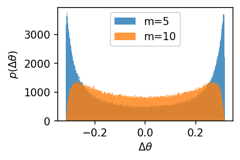
which is a (shifted and rescaled) sinusoidal distribution. This means that, when , is either very close to or very close to . We might even go one step further to see what happens if . For , , while for and , the limit is not well-defined. This is a signature that the distribution is tending to a mixed delta-distribution proportional to . The fact that this is not a well-defined limit suggests that there is a singularity in the variable when , and some qualitative transition has happened as we approach the limit. For , by definition we should obtain a delta distribution , which is what one expects.
Now we are ready to obtain the distribution for . Applying the transformation rule to Equation 21 (and extend the distribution from to ), we obtain
| (28) |
this is the predicted distribution of . We plot the theoretical p.d.f. in Figure 1. We may perform another transformation of variable to see that this is still distribution. As expected in Proposition 1, this distribution is bounded and sub-gaussian. Let , we see
| (29) |
where is the normalizing constant. This is a distribution, centered, and with a Gaussian asymptotic distribution.
Now we proceed to define and extend the support from to ; we obtain
| (30) |
Again, when ,
| (31) |
which is the Gaussian distribution. The more interesting case is also the non-asymptotic case. When , we have that
| (32) |
which is the sinusoidal distribution. When ,
| (33) |
which is a uniform distribution supported on .
To summarize, we have derived the major theoretical result of this work.
Theorem 1.
Let be i.i.d. sampled from , , and , , then the p.d.f. of is given by Equation 30.
It is interesting to compare this with the -distribution. While the -distribution is unbounded, this distribution is bounded for any finite . As , the two distributions converge to the same limiting Gaussian distribution with variance . The variance for at finite is , while that of the has variance , and we obtain the relation
| (34) |
and the inequality becomes equality when . This shows that approximating by neglecting the correlation between the numerator and denominator overestimates the variance; it also predicts to have the wrong trend: while the actual distribution has decreasing variance as decreases, the -distribution predicts increasing variance, with its variance diverging at .

Besides the p.d.f. for , the following two corollaries summarizes the most important predictions of this work. Agreement with the experiment would suggest that the assumptions made in this work are valid and applicable to real situations. The limitation is that these results hinge on the assumption that the gradient’s underlying distribution is a zero-mean Gaussian with a constant variance; the deviation between the theoretical distribution and the measured distribution can be used to probe the skewed-ness of the gradient, the existence of a correlation between the different parameters, and the time evolution of the variance.
Corollary 1.
The variance of is .
Corollary 2.
The variance of is
an increasing function of time and converges to a finite value as .
5 Experiments
In this section, we conduct experiments to test our theory. Notice that the experiments and plots are obtained from a single training trajectory instead of obtained by averaging over an ensemble of training trajectories with different initializations of the networks. We expect the agreement for all experiments to get even better when such ensembling is used. The fact that the agreement is right on a single trajectory level makes our theory more applicable to real problems (so that the practitioners only have to run once and check what went wrong). The agreement is expected to become better if we average over multiple runs.


5.1 Distribution the Update
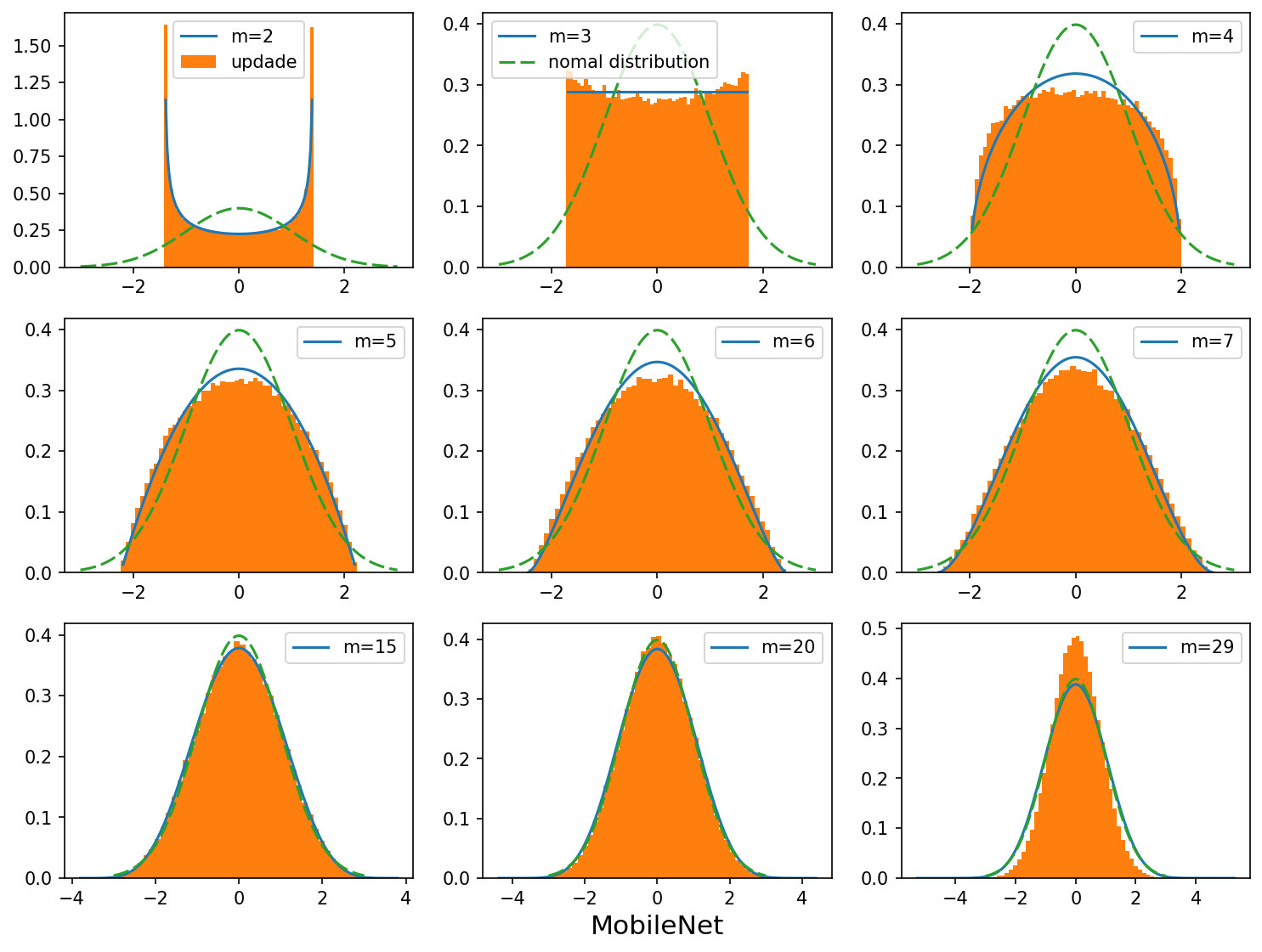
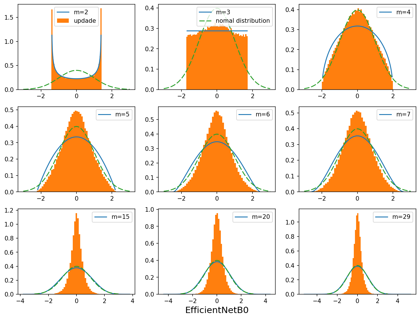
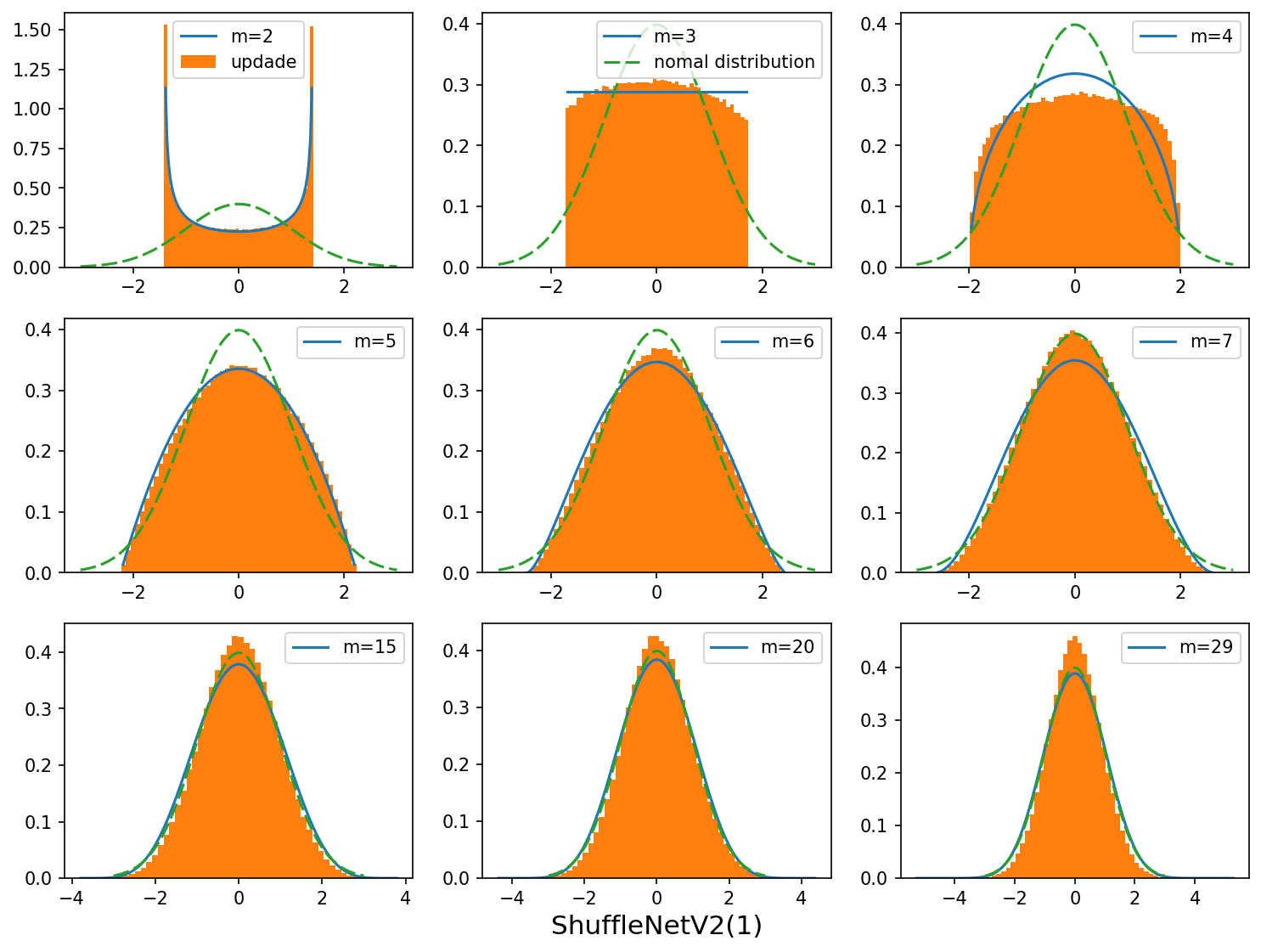
We measure the probability density function of the update of the adaptive gradient when we train on RegNetX-200MF [Radosavovic et al. 2020] on the CIFAR-10 dataset33 3 RegNetX is the newest generation of modern CNN architectures with state-of-the-art performance in computer vision. It is based on the residual structure [He et al. 2016]. See Figure 2. We see that the agreement between our prediction and experiment is good both quantitatively and qualitatively. Qualitatively, the following two predictions are confirmed: (1) the distribution transitions from a bi-modal distribution to a uni-modal distribution at increases; for this task, it is even more surprising that the transition to a uni-modal distribution occurs exactly at the predicted time step ; (2) the distribution converges to a gaussian distribution. A similar level of agreement is observed for all other layers of the network (see appendix); this suggests our assumptions’ general applicability and, therefore, our theory. One interesting point is that the empirical data seems slightly right-skewed. We hypothesize that this is because the underlying distribution of has a non-vanishing mean (also see our experiments in Section 6 for why this is the case). In the appendix, we also plot the single-trajectory update distribution for VGG [Simonyan and Zisserman 2014], ResNet-18 [He et al. 2016], ShuffleNet-V2 [Zhang et al. 2018], ResNeXt-29 [Xie et al. 2017], MobileNet [Howard et al. 2017], EfficientNet-B0 [Tan and Le 2019], and DenseNet-121 [Huang et al. 2017], which we show to also agree well with the prediction44 4 Some deviation is also observed, but such deviations seem to appear in a consistent way for a fixed architecture, suggesting that the actual distribution has some sensitivity to the model..
We also plot compare the distribution over different random initializations in Figure 8. We plot the overlap of three different random seed in dark red, which also agrees well with the prediction. We see that the variance of the distribution across different seeds is relatively small, and all agree well with the theoretical prediction.

5.2 Increasing and Bounded variance
One of the key predictions of this work is that the adaptive gradients’ variance is an increasing function of time when the training is not far from initialization, and we verify this prediction in this section. We plot the variance of the update versus the time step on CIFAR-10, for different model architectures: RegNetX, MobileNet [Howard et al. 2017], and ShuffleNet [Zhang et al. 2018]. See Figure 3. The agreement between our theory and experiment is excellent. There are two points worth noticing: (1) the agreement is very good for , suggesting that a constant Gaussian distribution well approximates the distribution of the gradient before this point; (2) there is no occasion when the variance of the update becomes anomalously large. This agreement suggests that (1) the distribution of gradient at initialization can be well-approximated by a time-independent gaussian at the initialization; (2) how far this approximation continues to hold as increases depends on the architecture of the model and the nature of the task. In the appendix, we show that there are also architectures that deviate from the predicted value from smaller values of , but they all have smaller variances than the predicted value, which further corroborates with the intended message that there is no problem with the variance of the adaptive gradients.
5.3 Distribution of the Transformer
In this section, we study the distribution of the original transformer architecture [Vaswani et al. 2017], since this is the situation where the distribution of the adaptive gradients is pathological. As in [Liu et al. 2019], we run transformer on the IWLST14 Ger-Eng dataset, using the default implementation in the Fairseq package [Ott et al. 2019]. See Figure 3-Right. We see that the transformer also has a very regular variance in the update, as expected by the theory. This suggests that the attribution of the pathological training behavior of transformers to the variance of Adam [Liu et al. 2019] is incorrect. We now show the empirical distribution of the updates in a single layer of the transformer architecture in Figure 4. We see that the distribution of the transformer is pathological and does not seem to obey a simple distribution. For example, at step (), there seem to be five prominent peaks in a single layer, which is a sign that the distribution is a composite one. Comparing with the experiment in Figure 5.LEFT and Figure 7, we hypothesize that there are at least two different underlying distributions: (1) a heavy-tail-like distribution feature the first, third, and fifth peak, and (2) a distribution with increasing variance featuring the second and the fourth peak. One essential future work is to investigate the cause of each of these peaks, which we believe, will shed new and important light on this poorly understood problem.
6 What affects the distribution of the update?
During training, it is often the case that the practitioners have to continually check the distribution of the gradient to infer what might be wrong with the training. For example, when the training of a model does not proceed well; one might suspect that it is due to (1) update too small; (2) update too large; or (3) update fluctuates too much, and these can only be known once one inspects the distribution of the update. Therefore, it is worth studying what might affect the distribution of the update. In our framework, this effect can incorporated by setting the variance of the underlying gradient distribution to be a function of time: . The distribution of the corresponding update no longer takes a simple analytic form now; therefore, we resort to simulations to answer this problem.
6.1 When is the update distribution bi-modal?
It is identified in [Liu et al. 2019] that the number of modes in the update distribution might affect ease of optimization, and the authors incorrectly attributed the cause to the divergence of the variance of the update. In this section, we show that the cause of bi-modality is the sudden increase of the variance of the gradient. See Figure 5. We experiment with the following two kinds of time-dependent gradient distribution: (1) ; (2) . We see that, in an increasing variance, the bi-modal structure remains for a relatively long time, while, in a decreasing variance, the bi-modal structure disappears very fast, and the distribution becomes thinner and sharper through time. This deformity can be compared with some real-task update distributions we encounter. For example, we plot the distribution of training a simple -layer CNN on MNIST in the appendix, where the bi-modal structure is shown to remain for a relatively long time; this suggests that, in this task, the variance of the gradient is increasing as time proceeds.


6.2 When is the distribution skewed?
Intuitively, the answer is simple: when the underlying distribution of has non zero-mean. Here, we do some numerical simulation to check what that will affect the distribution quantitatively. Here, we experiment with following two kinds of noise; since the distribution simply flips if we change the sign of the mean, we only simulate with negative mean value: (1) ; (2) . See Figure 6 for the result. We see that the resulting distribution is left-skewed but moves back towards the center as increases. It is also interesting to notice that the distribution gets thinner and less skewed when the magnitude of the mean increases with time.

6.3 Heavy-tailed gradient distribution
The gradient may take a heavy-tailed distribution55 5 There is increasing research interest in studying the case when the underlying gradient is heavy-tailed [Gurbuzbalaban et al. 2020, Simsekli et al. 2019]. It is not rare that the update distribution of real tasks shows a trimodal structure. Many figures in [Liu et al. 2019] suggest the existence of a trimodal structure when a transformer is trained on a machine learning task.. We simulate this by sampling from a standard Cauchy distribution. See Figure 7. Interestingly, the distribution takes a trimodal structure. This trimodality suggests that the update distribution’s trimodal structure may suggest (1) the existence of a large-norm but sparse gradient or (2) the training has very strong or even divergent noise. In fact, the update distribution for ResNet-18 and VGG21 are observed to be clearly bimodal at the initial step while the other studied models do not; see the appendix.
7 Concluding Remark
In this work, we studied the distribution of the update of the adaptive gradient methods. We showed that the variance of (any higher moment of, in fact) of the adaptive gradient method does not diverge. The variance of the update is a constant, and the variance of its magnitude is an increasing function of time; this, in turn, means that the adaptive gradient methods are surprisingly stable, especially at the beginning of training. Adam’s unexpected stability at initialization also implies that the previous understanding that the need for the warmup of Adam [Liu et al. 2019] is still an open problem. We believe that identifying the correct cause of Adam’s incapability to train transformers will ultimately benefit the community.
Implications. There are a few important implications of this work. Correlation of the gradient. Our analysis’s limitation is obvious, the most important one being that the gradient is assumed to be uncorrelated for different parameters; this assumption leads to the analytical formula we derived, which, intuitively, is unlikely to be the case for a non-linear system. What is surprising here is that a theory based on such limited theory agrees excellently with the experiments; this, in turn, implies that the gradient noises of minibatch SGD are likely well-approximated by a diagonal matrix. The reason behind this anomalous suppression of off-diagonal covariance should be a crucial topic to study in the future. Approximate Bayesian Inference. Knowing the posterior distribution of the iteration of the optimization algorithm has important application to approximate Bayesian inference, where SGD and Adam are used as MCMC algorithms for approximating the posterior distribution of the model parameters [Mandt et al. 2017, Liu et al. 2020, Ziyin et al. 2021], which are often useful for assessing the uncertainty in the model parameters.
References
- Barakat and Bianchi [2018] Anas Barakat and Pascal Bianchi. Convergence and dynamical behavior of the adam algorithm for non-convex stochastic optimization. arXiv preprint arXiv:1810.02263, 2018.
- Barakat and Bianchi [2020] Anas Barakat and Pascal Bianchi. Convergence rates of a momentum algorithm with bounded adaptive step size for nonconvex optimization. In Asian Conference on Machine Learning, pages 225–240. PMLR, 2020.
- Choi et al. [2020] Dami Choi, Christopher J. Shallue, Zachary Nado, Jaehoon Lee, Chris J. Maddison, and George E. Dahl. On empirical comparisons of optimizers for deep learning, 2020.
- da Silva and Gazeau [2018] André Belotto da Silva and Maxime Gazeau. A general system of differential equations to model first order adaptive algorithms. arXiv preprint arXiv:1810.13108, 2018.
- Devlin et al. [2018] Jacob Devlin, Ming-Wei Chang, Kenton Lee, and Kristina Toutanova. Bert: Pre-training of deep bidirectional transformers for language understanding. arXiv preprint arXiv:1810.04805, 2018.
- Duchi et al. [2011] John Duchi, Elad Hazan, and Yoram Singer. Adaptive subgradient methods for online learning and stochastic optimization. J. Mach. Learn. Res., 12:2121–2159, July 2011. ISSN 1532-4435. URL http://dl.acm.org/citation.cfm?id=1953048.2021068.
- Gurbuzbalaban et al. [2020] Mert Gurbuzbalaban, Umut Simsekli, and Lingjiong Zhu. The heavy-tail phenomenon in sgd. arXiv preprint arXiv:2006.04740, 2020.
- He et al. [2016] Kaiming He, Xiangyu Zhang, Shaoqing Ren, and Jian Sun. Deep residual learning for image recognition. In Proceedings of the IEEE conference on computer vision and pattern recognition, pages 770–778, 2016.
- Howard et al. [2017] Andrew G Howard, Menglong Zhu, Bo Chen, Dmitry Kalenichenko, Weijun Wang, Tobias Weyand, Marco Andreetto, and Hartwig Adam. Mobilenets: Efficient convolutional neural networks for mobile vision applications. arXiv preprint arXiv:1704.04861, 2017.
- Huang et al. [2017] Gao Huang, Zhuang Liu, Laurens Van Der Maaten, and Kilian Q Weinberger. Densely connected convolutional networks. In Proceedings of the IEEE conference on computer vision and pattern recognition, pages 4700–4708, 2017.
- Jiwoong Im et al. [2016] D. Jiwoong Im, M. Tao, and K. Branson. An empirical analysis of the optimization of deep network loss surfaces. ArXiv e-prints, December 2016.
- Kingma and Ba [2014] Diederik P. Kingma and Jimmy Ba. Adam: A method for stochastic optimization. CoRR, abs/1412.6980, 2014. URL http://dblp.uni-trier.de/db/journals/corr/corr1412.html#KingmaB14.
- Lan et al. [2019] Zhenzhong Lan, Mingda Chen, Sebastian Goodman, Kevin Gimpel, Piyush Sharma, and Radu Soricut. Albert: A lite bert for self-supervised learning of language representations. arXiv preprint arXiv:1909.11942, 2019.
- Le et al. [2011] Quoc V Le, Jiquan Ngiam, Adam Coates, Ahbik Lahiri, Bobby Prochnow, and Andrew Y Ng. On optimization methods for deep learning. In ICML, 2011.
- Liu et al. [2020] Kangqiao Liu, Liu Ziyin, and Masahito Ueda. Stochastic gradient descent with large learning rate. arXiv preprint arXiv:2012.03636, 2020.
- Liu et al. [2019] Liyuan Liu, Haoming Jiang, Pengcheng He, Weizhu Chen, Xiaodong Liu, Jianfeng Gao, and Jiawei Han. On the variance of the adaptive learning rate and beyond. arXiv preprint arXiv:1908.03265, 2019.
- Loshchilov and Hutter [2017] Ilya Loshchilov and Frank Hutter. Fixing weight decay regularization in adam. arXiv preprint arXiv:1711.05101, 2017.
- Luo et al. [2019] Liangchen Luo, Yuanhao Xiong, Yan Liu, and Xu Sun. Adaptive gradient methods with dynamic bound of learning rate. In Proceedings of the 7th International Conference on Learning Representations, New Orleans, Louisiana, May 2019.
- Ma and Yarats [2019] Jerry Ma and Denis Yarats. On the adequacy of untuned warmup for adaptive optimization. arXiv preprint arXiv:1910.04209, 2019.
- Mandt et al. [2017] Stephan Mandt, Matthew D Hoffman, and David M Blei. Stochastic gradient descent as approximate bayesian inference. arXiv preprint arXiv:1704.04289, 2017.
- Nesterov [1983] Yurii E Nesterov. A method for solving the convex programming problem with convergence rate . In Dokl. akad. nauk Sssr, volume 269, pages 543–547, 1983.
- Ott et al. [2019] Myle Ott, Sergey Edunov, Alexei Baevski, Angela Fan, Sam Gross, Nathan Ng, David Grangier, and Michael Auli. fairseq: A fast, extensible toolkit for sequence modeling. In Proceedings of NAACL-HLT 2019: Demonstrations, 2019.
- Popel and Bojar [2018] Martin Popel and Ondřej Bojar. Training tips for the transformer model. The Prague Bulletin of Mathematical Linguistics, 110(1):43–70, 2018.
- Radosavovic et al. [2020] Ilija Radosavovic, Raj Prateek Kosaraju, Ross Girshick, Kaiming He, and Piotr Dollár. Designing network design spaces. In Proceedings of the IEEE/CVF Conference on Computer Vision and Pattern Recognition, pages 10428–10436, 2020.
- Reddi et al. [2018] Sashank Reddi, Satyen Kale, and Sanjiv Kumar. On the convergence of adam and beyond. In International Conference on Learning Representations, 2018.
- Simonyan and Zisserman [2014] Karen Simonyan and Andrew Zisserman. Very deep convolutional networks for large-scale image recognition. arXiv preprint arXiv:1409.1556, 2014.
- Simsekli et al. [2019] Umut Simsekli, Levent Sagun, and Mert Gurbuzbalaban. A tail-index analysis of stochastic gradient noise in deep neural networks. arXiv preprint arXiv:1901.06053, 2019.
- Sun [2019] Ruoyu Sun. Optimization for deep learning: theory and algorithms. arXiv preprint arXiv:1912.08957, 2019.
- Tan and Le [2019] Mingxing Tan and Quoc V Le. Efficientnet: Rethinking model scaling for convolutional neural networks. arXiv preprint arXiv:1905.11946, 2019.
- Tieleman and Hinton [2012] T. Tieleman and G. Hinton. Lecture 6.5—RmsProp: Divide the gradient by a running average of its recent magnitude. COURSERA: Neural Networks for Machine Learning, 2012.
- Vaswani et al. [2017] Ashish Vaswani, Noam Shazeer, Niki Parmar, Jakob Uszkoreit, Llion Jones, Aidan N Gomez, Łukasz Kaiser, and Illia Polosukhin. Attention is all you need. In Advances in neural information processing systems, pages 5998–6008, 2017.
- Xie et al. [2017] Saining Xie, Ross Girshick, Piotr Dollár, Zhuowen Tu, and Kaiming He. Aggregated residual transformations for deep neural networks. In Proceedings of the IEEE conference on computer vision and pattern recognition, pages 1492–1500, 2017.
- Young et al. [2018] Tom Young, Devamanyu Hazarika, Soujanya Poria, and Erik Cambria. Recent trends in deep learning based natural language processing. ieee Computational intelligenCe magazine, 13(3):55–75, 2018.
- Zhang et al. [2018] C. Zhang, Q. Liao, A. Rakhlin, B. Miranda, N. Golowich, and T. Poggio. Theory of Deep Learning IIb: Optimization Properties of SGD. ArXiv e-prints, January 2018.
- Zhang et al. [2018] Xiangyu Zhang, Xinyu Zhou, Mengxiao Lin, and Jian Sun. Shufflenet: An extremely efficient convolutional neural network for mobile devices. In Proceedings of the IEEE conference on computer vision and pattern recognition, pages 6848–6856, 2018.
- Ziyin et al. [2020] Liu Ziyin, Zhikang T Wang, and Masahito Ueda. Laprop: a better way to combine momentum with adaptive gradient. arXiv preprint arXiv:2002.04839, 2020.
- Ziyin et al. [2021] Liu Ziyin, Kangqiao Liu, Takashi Mori, and Masahito Ueda. On minibatch noise: Discrete-time sgd, overparametrization, and bayes, 2021.
Appendix A Additional Experiments
A.1 Distribution across different random seeds
We also plot compare the distribution over different random initializations in Figure 8. We plot the overlap of three different random seed in dark red, which also agrees well with the prediction. We see that the variance of the distribution across different seeds is relatively small, and all agree well with the theoretical prediction.

A.2 Other Experiments on CIFAR-10
In this section, we present more experiments to validify our theory. We first plot the distribution of update for a different layer (from what appeared in the main text) RegNetX-200MF trained on CIFAR-10, and excellent agreement between our theory and experiment is observed. We then plot the distribution of updates from random layers (with more than parameters) of VGG [Simonyan and Zisserman 2014], ResNet-18 [He et al. 2016], ShuffleNet-V2 [Zhang et al. 2018], ResNeXt-29 [Xie et al. 2017], MobileNet [Howard et al. 2017], EfficientNet-B0 [Tan and Le 2019], DenseNet-121 [Huang et al. 2017]. We first plot the variance of and in Figure 9. While some nets deviate from the theory, others agree quite well. For those that deviate from the prediction, we observe that they all have smaller variances than the predicted value, this agrees with our message that the adaptive gradient methods do not have exploding variance problem at the beginning of training. We then plot the distributions of for a single trajectory for each of these models.