Efficient Least Squares Monte-Carlo Technique for PFE/EE Calculations
Abstract
We describe a regression-based method, generally referred to as the Least Squares Monte Carlo (LSMC) method, to speed up exposure calculations of a portfolio. We assume that the portfolio contains several exotic derivatives that are priced using Monte-Carlo on each real world scenario and time step. Such a setting is often referred to as a Monte Carlo over a Monte Carlo or a Nested Monte Carlo method.
Keywords American Monte-Carlo Least-Squares Monte-Carlo AMC LSMC Nested Simulation
1 Introduction
Least Squares Monte-Carlo (LSMC) is a technique based on least squares regression, which we describe in this paper. We think of LSMC as a special case of a larger class of methods that are referred to as American Monte-Carlo in the literature [1], [2]. The term AMC has its origins in the work of Longstaff and Schwartz [3]. Therein, the authors describe a method to price American Options that relies on building a conditional expectation function using a least squares regression technique over a set of explanatory variables. In the simplest case, the set of explanatory variables would include the current state of the underlying risk factors. In its original form, the method uses two sets of Monte-Carlo simulations. One simulation is used to build the conditional expectation function by regressing over the stock price and the indicator that the option is in the money using backward propagation of state variables. Once the backward pass is done, a different set of Monte-Carlo paths are used to move forward to price the instrument. During the forward pass, the already constructed conditional expectation functions are used at every observation date to determine whether it is optimal to exercise or not.
In its modern usage, in the context of risk management, the term AMC (or LSMC) is used to handle the Nested Monte-Carlo (NMC). As an illustration, consider Potential Future Exposure (PFE) or Expected Exposure (EE) for a portfolio consisting of exotic instruments.11 1 For detailed example of PFE and EE see [4]. To estimate an EE and PFE profiles, we value the portfolio on a set of future market, or “outer”, scenarios generated across time. Suppose we use 5,000 such scenarios, and use 5,000 risk-neutral, “inner”, paths to obtain a single price estimate on each outer scenario. Under this set-up, the computational cost for each exotic instrument will be proportional to on each time step. Clearly, we need to apply some clever techniques to reduce the computation cost.
One such solution has been proposed by Barrie and Hibbert [5]. Berrie and Hibbert’s method reduces the overall computational cost by decreasing the number of inner paths. Their method aims at reducing Monte-Carlo errors by regressing the estimated prices against a set of explanatory variables generated in the outer loop. We refer to price estimates obtained using this method as LSMC price estimates. To illustrate the LSMC method, consider a vanilla call option under Geometric Brownian Motion with constant drift and volatility. We use a GBM model in the outer loop to generate a set of underlying stock prices and use GBM model within the inner loop to price the option. Assume that the option matures in one year (time step 360), and we are interested in computing prices at time steps 15, 30, …, 360. On each time step, in a typical NMC setting, we use 5,000 inner paths to obtain MC price estimates. Under the LSMC setting, we use 30 inner paths, for example, per outer scenario to obtain a set of MC prices on a given time step. When these prices are plotted against 5,000 underlying (outer) spot values on a given time step, we expect to see some relationship. We assume that this relationship can be explained by
| (1.1) |
where is the MC price, is the spot price of the equity, and is the error on the scenario.
Once the preliminary simulation is done, we have 5,000 MC price estimates and 5,000 spot values that we use to build regression model (1.1) to obtain coefficient estimates . These coefficient estimates are then used to obtain LSMC price estimates given by
Figure 1 compares the LSMC price estimates to the Black-Scholes analytic prices. The graphs are provided for time steps 15 and 345. In order to obtain the “hockey stick” shape near maturity of the option, we incorporate a dummy variable
into equation (1.1) to yield
| (1.2) |
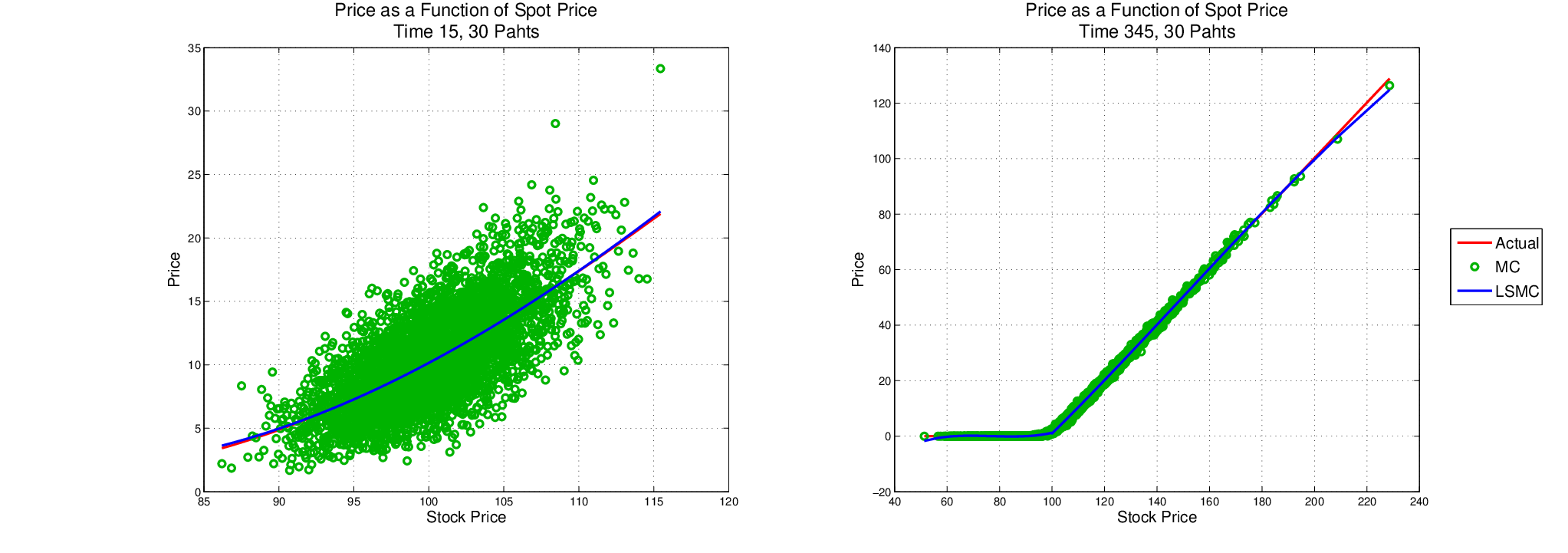
Figure 1 reveals that the LSMC price estimates are much closer to the true analytic prices than the original MC prices. Interestingly enough, Barrie and Hibbert’s method can be viewed as a variance reduction technique, though it was not presented as such in their original report. In this paper we look at the method more closely and present a variance formulation that could be used to evaluate the accuracy of price estimates. We also look at the PFE and EE profiles for a set of exotic instruments to test the accuracy of this method.
2 Least Squares Monte-Carlo
We assume, at outset, that Monte-Carlo scenarios have been generated over time points in the set , where , for . These time points may represent important dates such as payment dates, fixing dates, etc. At any time , we have vectors , for , representing the cross sectional information obtained from the scenarios at time and absorbing all the information up to time . These vectors form the explanatory variables for the regression model for time .
Suppose that we are interested in obtaining the time price of an exotic instrument maturing at time . If denotes the discounted payoff of this instrument, then the time price is obtained under the conditional expectation
| (2.1) |
One can estimate the integral on the right-hand-size of equation (2.1) using a MC method. Doing so, will generate a sequence of MC estimates , at each time . These prices form the corresponding set of response variables for our regression model. We can write the relationship as
| (2.2) |
where are coefficients of expansion (as in equation (1.1))) and are basis functions (as in equation (1.1)). We obtain MC prices by computing the mean of generated discounted payoffs in the inner loop. Specifically,
| (2.3) |
where is generated under risk neutral measure, and is the value of the discounted payoff function on the path. The Monte-Carlo price can represented as the sum of the true value and a Monte-Carlo error , or
| (2.4) |
Now, suppose we let in equation (2.2), then
| (2.5) |
As the number of paths tends to infinity, will approach . 22 2 by the Strong Law of Large Numbers. In case of a perfect model, equals zero. Generally, is measurable (deterministic) and is often a function of . From equation (2.5), we conclude that
| (2.6) |
Substituting the right-hand-side of equation (2.6) into equation (2.4) yields the final model
The total error from equation (2.2) can be viewed as the sum of deterministic part and a random part . In practice, we do not observe directly nor can accurately measure unless we use high number of paths. However, we can estimate the variance of using the discounted payoff.
For sufficiently large number of paths, follows normal distribution with mean and . The non-biased estimator for then is given by
| (2.7) |
In case , the MC variance estimator becomes
In a matrix notation, we can write the regression model (2.2) as
| (2.8) |
then, the coefficient estimator becomes
and
with
is also known as an orthogonal projection. Conquently, the total variance of is lower than the total variance of . This is given by the following theorem and is proven in appendix A.
Theorem 2.1.
Let be a random vector having a finite variance, and let be an orthogonal projection onto a linear subspace of . Then,
where denotes the trace operator.
By Theorem 2.1, we know that the total variance reduction is expected under an orthogonal projection
| (2.9) |
where represents the covariance matrix of that is estimated using the discounted payoffs generated in the inner loop. Furthermore, when the covariance matrix is equal to for some constant the ratio of total LSMC variance and total MC variance is given by
which follows from the properties of .
3 Illustrative Results
In this section, we test the accuracy of the LSMC methodology. An Arithmetic Asian Option is used to check the fit of various degree polynomials. After we obtain a good fit, we look at the EE and PFE profiles of a Barrier Option, Target Accrual Redemption Note, Accumulating Forward Contract and Asian Option. For the reader’s convenience, we describe the payoffs of these instruments in appendix B.
3.1 LSMC Analysis
Consider an Arithmetic Asian Put Option that matures at time with time fixings and weights . The payoff at maturity takes the form
| (3.1) |
where is the price of the underlying equity at time . For simplicity, assume that follows a GBM with constant drift and volatility in the outer and inner loops.33 3 The drift in the outer loop is set at 0.1, while the drift in the inner loop is set at 0.05. Let the observation time be for . We consider orthogonal Forsythe polynomials [6] for basis functions using as the explanatory variable in the regression model. We perform the following steps to obtain LSMC estimates:
- •
Transform the explanatory variables to take values between and using
- •
Obtain regression matrix using Forsythe polynomial expansion
- •
Estimate the coefficients in model (2.8)
- •
Use the coefficient estimates to obtain LSMC prices
We set a numerical experiment with 1, 10, 30, 50, 100 and 10,000 inner paths to compute and regress against to get . To study the accuracy of the fit and variance reduction, we compare LSMC estimates to MC prices obtained using Sobol paths. The results are summarized in Figures2 3 and 4.
First time step fit using polynomial of degree five

Note that fully estimated covariance matrix was used to obtain the ratio of total of MC variance and total of LSMC variance. As one can see, the ratio of total of MC to LSMC variance is close to . That is, using regression, we are able to reduce the variance by about 99.9%.
First time step

From Figure 2, one may infer that we can obtain very accurate price estimates using 10 paths per outer scenario. Then, assuming that a typical Nested Monte-Carlo requires 5,000 inner paths to get a reasonable PFE and EE profile, we can speed up the computation by a factor of 500 using LSMC. Furthermore, one can argue that a higher polynomial degree could provide a better fit. Though this may be true when one is dealing with a closed-form functional approximation, high-degree polynomials tend to overfit data with noise. These results are most evident in Figure 5, where we plot the sum of squared deterministic residuals (SSE) .
First time step fit using polynomial of degree five

Let , , , , be the Actual value, the Actual fit, MC price and LSMC price, respectively. Figure 5 compares SSE values computed with
First time step fit with varying degree polynomials

We define Actual fit as the least squares fit of price estimates computed using a large number () of Sobol paths. The SSE of Actual fit that has been computed using has a very small (quasi) MC error and serves as a measure of accuracy. From Figure 5, we observe monotonic decrease of SSE when we select higher degree polynomials for the Actual fit. This does not happen when we fit data with noise. In general, the less accurate are the price estimates, the sooner SSE starts to increase. That is, higher degree polynomials tend to overfit data with noise. With that in mind, we use the third degree polynomial for PFE and EE estimation: it appears to be the highest degree at which SSE does not increase in the graphs presented.
3.2 PFE and EE Results
For PFE and EE computations, we use a joint Hull-White two-factor model for interest rates and Heston stochastic volatility model for FX and Equity to generate outer, real scenarios. We use different models for pricing, which vary depending on the instrument. Table 1 summarizes the risk-neutral models used in the inner loop for each instrument. For computational efficiency, with no loss of generality, all instruments mature in one year and have fixing dates set at 15 day intervals. The profiles obtained for PFE and EE per instrument are summarized in Figures 6 and 7, respectively.
| Instrument | Model | Underlying |
|---|---|---|
| Asian | Hull-White-Black-Scholes | Foreign Exchange |
| Forward | Geometric Brownian Motion | Equity |
| Barrier | Hull-White-Black-Scholes | Foreign Exchange |
| TARN | Libor Market Model | Libor Rate |


The PFE and EE profiles for the Actual data series in Figures 6 and 7 are obtained using 4096 Sobol paths in the inner loop. For the LSMC PFE and EE profiles, we used varying numbers of paths that were determined by numerical experiments. We found that smooth instruments such as Asian, TARN and Accumulative Forward require smaller numbers of paths. In most cases, we were able to obtain fairly accurate price estimates using anywhere between 10 and 30 inner paths. To get accurate LSMC Barrier price estimates, we used anywhere between 30 and 64 inner paths. On average, we were able to speed up the computation of PFE and EE profiles by a factor of 60.
4 Conclusion
In this paper, we were able to show that the least squares Monte-Carlo approach proposed by Barrie and Hibbert, can capture the tails of the distribution with a high degree of accuracy. This method, however, does call for numerical experiments for model calibration where an appropriate number of inner paths and basis functions need to be selected. Though we were able to capture all instrument prices with third degree polynomial basis functions, one should exercise care and diligence when selecting a higher degree. As mentioned previously, high-degree polynomials may overfit data with noise, which would result in worse price estimates.
In this paper, we have also proved that the total variance of the least squares estimates is no greater than the total variance of the original MC estimates. Indeed, this result should be anticipated since the LSMC method can be viewed as a smoothing method. Our current results suggest that LSMC should perform better in aggregate risk metrics such as CVA and/or CVA sensitivity, which is a topic for a future study.
Acknowledgement
We express special thanks to Ian Isoce for checking the main result and the time spent in numerous discussions. We also thank Raymond Lee for helping to produce numerical results, and Alejandra Premat for suggesting credit risk metrics.
Appendix A Least Squares Linear Regression
In this section we review the linear regression model and a reduction of variance theorem. Linear regression modelling and estimation techniques can be found in many linear regression textbooks such as [7]. We start with a linear regression model of the form
| (A.1) |
with a response variable , regression variables and error terms . The least squares estimator is the solution to
| (A.2) |
where is -norm of vector . The solution to problem (A.2) is given by , and the estimator of is
| (A.3) |
provided that is invertible.
, commonly known as the hat matrix, maps the response variables onto by minimizing the sum of squared errors . is also the orthogonal projection onto the column space of . Clearly, is symmetric and idempotent.
We can also look at the problem (A.1) from a statistical point of view and compute the variance of our mean estimator . Suppose is a random vector with finite variance, then the covariance of the mean response is given by
| (A.4) |
where is the covariance matrix of . Furthermore, we can conclude that the total variance of the mean response estimator is less than or equal to the total variance of the original vector by the following theorem.
Theorem.
Let be a random vector having a finite variance, and let be an orthogonal projection onto a linear subspace of . Then,
where denotes the trace operator.
Proof.
Expressing , then
by properties of and operator. ∎
Appendix B Definition of Instruments
B.1 Notation
- •
denotes the price of the underlying at time .
- •
denotes a stopping time.
- •
.
- •
is maturity of the instrument unless otherwise stated.
- •
.
- •
.
B.2 Payoff Functions
- •
K-Strike Arithmetic Asian Option with weights :
put call - •
K-Strike Up-and-Out Barrier Option with barrier and rebate :
put call where . The rebate is paid at time and is paid at maturity.
- •
Accumulating Forward Contract with n-payments and barrier :
short long where
- •
Target Accrual Redemption Note with barrier on accrual payments, LIBOR rate and fixed rates and :
receiver payer where .
References
- [1] Samim Ghamami and Bo Zhang. Efficient Monte Carlo Counterparty Credit Risk Pricing and Measurement. Technical report, Federal Reserve, 2014.
- [2] Alexander Sokol. Long Term Portfolio Simulation for XVA, Limits, Liquidity and Regulatroy Capital. Risk Books, July 2014.
- [3] Francis A. Longstaff and Eduardo S. Schwartz. Valuing American Options by Simulation: A Simple Least-Sqaures Approach. The Review of Financial Studies, pages 113–147, 2001.
- [4] Ignacio Ruiz. XVA Desks - A New Era for Risk Management. Palgrave Macmillan, 2015.
- [5] Adam Koursaris. A Least Squares Monte Carlo Approach to Liability Proxy Modelling and Capial Calculation. Technical report, Barrie & Hibbert; A Moody’s Analytics Company, September 2011.
- [6] George E. Forsythe. Generation and use of orthogonal polynomials for data fitting with a digital computer. Journal of the Society of Industrial Applied Mathematics, pages 74–88, May 1957.
- [7] George A. F. Seber and Alan J. Lee. Linear Regression Analysis. John Wiley & Sons, Inc, 2003.