跳到论文正文
W Papers独立论文阅读器 arXiv:2105.07047 论文正文 计算阅读时间 · 0%
引用这篇论文根据当前论文元数据生成,正式投稿前建议核对。


License: arXiv.org perpetual non-exclusive license
arXiv:2105.07047v1 [eess.SP] 14 May 2021

On Performance of Energy Harvested Cooperative NOMA Under Imperfect CSI and Imperfect SIC

Shubham Bisen    Parvez Shaik    Vimal Bhatia Thanks: Shubham Bisen, Parvez Shaik and Vimal Bhatia are with the Discipline of Electrical Engineering, Indian Institute of Technology Indore, Indore 453552, India (e-mail: {phd1901202001; phd1601202003; vbhatia}@iiti.ac.in.)
Abstract

With the advent of 5G and the need for energy-efficient massively connected wireless networks, in this work, we consider an energy harvesting (EH) based multi-relay downlink cooperative non-orthogonal multiple access (NOMA) system with practical constraints. The base station serves NOMA users with the help of decode-and-forward based multiple EH relays, where relays harvest the energy from the base station’s radio frequency. A relay is selected from the multiple K-relay by using a partial relay selection protocol. The system is considered to operate in half-duplex mode over a generalized independent and identical Nakagami−m-m fading channel. The closed-form expression of outage probability and ergodic rate are derived for users, under the assumption of imperfect channel state information (CSI) and imperfect successive interference cancellation (SIC) at the receiver node. Expression of outage probability and ergodic rate for both users under the assumption of perfect CSI and perfect SIC are also presented. Further, the asymptotic expression for the outage probability is also shown. The derived analytical expressions are verified through Monte-Carlo simulations.

Index Terms: 
NOMA, Energy harvesting, Nakagami−m-m fading, outage probability, asymptotic outage, ergodic rate.

I Introduction

5t​h5^{th} generation (5G) wireless communication standard is drafted by the third generation partnership project to meet the growing demands of multi-rates data applications. Non-orthogonal multiple access (NOMA) is one of the leading beyond 5G technologies and is considered a prominent and promising solution with superior spectrum efficiency and massive connectivity [1, 2, 3]. Recently, cooperative relaying and the NOMA system have gained research attention due to its significant and prominent advantages in improving the coverage and reliability. [4, 5, 6, 7, 8, 9, 10, 11]. In [5], authors investigated cooperative-NOMA with amplify-and-forward (AF) and decode-and-forward (DF) relaying and derived the outage probability and asymptotic outage probability expressions. Considering the fact that multiple relays provide a significant performance gain in cooperative networks, special attention has been given to the cooperative NOMA with multiple relays and analysis of relay selection techniques [7, 8, 9, 10]. In [7], the authors have provided a two-stage max-min relay selection scheme for the NOMA system with fixed power allocation at relays and different quality of service (QoS) requirements at users. In [7], the users are selected based on different QoS requirements, whereas in [8], authors have considered the users according to their channel condition, with fixed and adaptive power allocation at the relay node. In [9], the outage probability of cooperative NOMA with multiple half-duplex DF relays is analyzed. In [10], the outage probability and sum rate of cooperative NOMA with multiple half-duplex AF relays were studied, considering partial relay selection (PRS). Energy harvesting (EH) from radio frequency signals is considered a viable solution to provide additional lifespan to energy-constrained nodes. Hence, EH based NOMA systems have gained research attention to meet the needs of 5G and beyond communications. In [12, 13, 14, 15, 16, 17], the performance of cooperative NOMA has been studied with EH relaying. A cooperative NOMA with simultaneous wireless information and power transfer is studied in [12], where nearby users acting as EH relays assist the far away NOMA users. In [13], authors analyzed the performance of cooperative NOMA network with EH relaying over Rayleigh fading. In [14], a multi-user NOMA system is analyzed with an EH powered relay node. In [15], the authors evaluated the NOMA system’s performance with multiple EH relaying and derived the closed-form expressions of outage probability and ergodic capacity over the Rayleigh fading channel. In [16], the authors analyzed the NOMA system’s outage probability with multiple EH AF relays with imperfect CSI and hardware impairment.
In the literature, most of the work assumes perfect knowledge of the channel state information (CSI) at the receiver, which is too idealistic for a practical system. However, in practice, knowledge of perfect CSI is unavailable at the receivers, which leads to channel estimation error (CEE). CEE significantly deteriorates the performance of the system [18, 19, 16]. In [18], a closed-form expression of outage probability is derived of a downlink relay aided NOMA system with multiple users over Nakagami-mm fading with imperfect CSI.

Contributions

To the best of the author’s knowledge, the NOMA system’s performance with decode-and-forward (DF) based multiple EH relays over Nakagami−m-m fading channels has not been considered. Further, a detailed study on the impact of practical constraint, imperfect CSI at receiver nodes, and imperfect SIC is not available in the literature. Nakagami-mm fading is considered due to its generalization to a variety of realistic fading channels, which includes Rayleigh fading channel with mm = 1, recently for THz channels with mm = 3 [20], and also for the unmanned aerial vehicle (UAV) [21]. The main contributions of this work are:

  • •

    For the first time in EH based multi-relay NOMA system, we consider the practical case of imperfect CSI at receiver nodes and imperfect SIC, and its impact on the system is analyzed.

  • •

    We present a DF based cooperative multiple EH relay based NOMA system employing relay selection and analyze its performance in terms of outage probability by deriving its closed-from expression from the novel end-to-end (e2e) SNR of the considered system for both users for both perfect and imperfect cases.

  • •

    Further, we analyzed the system performance at high SNR by deriving the expression of asymptotic outage probability and useful insights are drawn.

  • •

    We optimized the EH time fraction parameter (α\alpha) to maximize the system throughput. The optimization problem is solved by adopting the particle swarm optimization (PSO) under both perfect and imperfect CSI/SIC conditions.

  • •

    Rate analysis of the system is performed by deriving the closed-form expression of ergodic rate for both users and the impact of imperfect CSI and SIC is analyzed.

The rest of the paper is organized as follows: the system model is introduced in Section II. Outage probability analysis is presented in Section III. Asymptotic outage probability analysis is presented in Section IV. Ergodic rate is analyzed in Section V. Numerical and simulation results are discussed in Section VI. Finally, in Section VII, conclusions are drawn.
Notation: Γ⁡(⋅)\text{$\Gamma$}(\cdot) is gamma function, G​mnpq​(a1,…,apb1,…,bp|x)G\begin{smallmatrix}m&n\\ p&q\end{smallmatrix}\left(\begin{smallmatrix}a_{1},\ldots,a_{p}\\ b_{1},\ldots,b_{p}\end{smallmatrix}\middle|x\right) is MeigerG function. Square of the norm is denoted by |⋅|2|\cdot|^{2}. Complex Gaussian distribution with mean 0, variance σ2\sigma^{2} is denoted by 𝒞​𝒩​(0,σ2)\mathcal{CN}(0,\sigma^{2}) and modified Bessel function of second kind of order nn is denoted by Kn​(⋅)K_{n}(\cdot). Expectation operator is denoted by E​(⋅)\text{E}(\cdot). Gaussian random variable (RV) with mean μ\mu and variance σ2\sigma^{2} is represented as 𝒩⁡(μ,σ2)\mathcal{N}({\mu,\sigma^{2}}). Probability density function (PDF) and cumulative distribution function (CDF) are given by f⁡(⋅)f(\cdot) and F⁡(⋅)F(\cdot), respectively. Factorial is denoted by (⋅)!(\cdot)!.

II System Model

R1R_{1}R2R_{2}RKR_{K}U1U_{1}U2U_{2}SSourcehrk,2h_{r_{k},2}hrk,1h_{r_{k},1}hs,r1h_{s,r_{1}}hs,r2h_{s,r_{2}}hs,rKh_{s,r_{K}}
Fig. 1: NOMA system with multiple EH relays

We consider a downlink cooperative NOMA system with EH-multiple relays as shown in Fig. 1, where a transmitter (S)(S), i.e., the base station (BS) transmits messages to the downlink users, i.e., U1U_{1} and U2U_{2}, with the help of cooperative relaying [7, 8]. Both users are ordered according to their channel condition. It is assumed that the weak users (U2U_{2}) is with poor channel condition and strong users (U1U_{1}) is with good channel condition. To facilitate cooperative relaying, it is also assumed that there are K numbers of relays in the system with DF relaying. Further, it is assumed that each node is equipped with a single antenna and operates in half-duplex mode. All the channel links are considered to be independent and identically distributed (i.i.d), which are modeled by Nakagami−m-m fading, the channel coefficients corresponding to links are represented as hi,jh_{i,j}, i∈(s,rk)i\in(s,r_{k}) and j∈(rk,1,2)j\in(r_{k},1,2), where the subscript s,rk,1s,r_{k},1 and 22 represent BS, RkR_{k}, U1U_{1} and U2U_{2} respectively. The |hi,j||h_{i,j}| is assumed to be Nakagami−m-m with shape parameter mi,jm_{i,j} and variance E⁡[|hi,j|2]=λi,jE[|h_{i,j}|^{2}]=\lambda_{i,j}. Under imperfect CSI, according to minimum mean squared error (MMSE) estimation [22, 23, 24],

hi,j=h^i,j+ϵi,j,h_{i,j}=\hat{h}_{i,j}+\epsilon_{i,j}, (1)

where hi,jh_{i,j} is actual channel and h^i,j\hat{h}_{i,j} is the estimate of the channel hi,jh_{i,j}, where hi,jh_{i,j} and h^i,j\hat{h}_{i,j} are jointly ergodic and stationary Gaussian process [25]. The ϵs,r\epsilon_{s,r} is the CEE, which is assumed to be complex normal with mean zero and variance σe2\sigma^{2}_{e}[26]. Assuming that h^i,j\hat{h}_{i,j} and ϵi,j\epsilon_{i,j} are independent11 1 The independence of h^i,j\hat{h}_{i,j} and ϵi,j\epsilon_{i,j} was not required, only that they were uncorrelated [22]., thus the estimated channel variance is given as λ^i,j=λi,j−σe2\hat{\lambda}_{i,j}=\lambda_{i,j}-\sigma_{e}^{2} [27].
In this work, the partial relay selection scheme (PRS) is considered for the selection of relay node, where the BS selects the relay which provides the best instantaneous channel gain between the BS and relay [28]. The BS continuously monitors the quality of the links between the BS and relays and based on this information, the source selects the best link. The PRS scheme to select the best source to relay link is expressed as |h^s,r|2=arg⁡maxk=1,2,…,K⁡|h^s,rk|2|\hat{h}_{s,r}|^{2}=\arg\max\limits_{k=1,2,...,K}|\hat{h}_{s,r_{k}}|^{2}.
Furthermore, relays harvest the energy from the source transmitted signal. In this paper, we considered the time switching (TS) protocol to harvest energy for α​T\alpha T block time, where α\alpha (0≤α≤1)(0\leq\alpha\leq 1) is the fraction of block time over which relay harvest the energy from a source transmitted signal. The remaining (1−α)​T(1-\alpha)T block time is assigned for the information transfer. The information transfer completes in two blocks, the first half of time block (1−α)​T2(1-\alpha)\frac{T}{2} is assigned for source to relay transmission, and the remaining half (1−α)​T2(1-\alpha)\frac{T}{2} for relay to users transmission. Thus, the harvested energy for α​T\alpha T time is given by [29] EH=Ps​μ​|h^s,r|2​α​TE_{H}=P_{s}\mu|\hat{h}_{s,r}|^{2}\alpha T, where 0≤μ≤10\leq\mu\leq 1 denotes energy conversion efficiency. The transmit power at RkR_{k} is expressed as Pr=EH(1−α)​T/2=2​Ps​μ​|h^s,r|2​α1−α.P_{r}=\frac{E_{H}}{(1-\alpha)T/2}=\frac{2P_{s}\mu|\hat{h}_{s,r}|^{2}\alpha}{1-\alpha}. Initially, BS transmits the NOMA signal for users by performing power domain multiplexing and superposition coding. The transmitted signal is given by xs=∑i=12ai​xix_{s}=\sum_{i=1}^{2}\sqrt{a_{i}}{x_{i}}, where, xi{x_{i}} denotes complex modulated symbols with unit energy for UiU_{i} (i.e., E​{|xi|2}=1\text{E}\left\{|x_{i}|^{2}\right\}=1). Further, aia_{i} is the power allocation coefficients for xix_{i} with ∑i=12ai=1\sum_{i=1}^{2}a_{i}=1 and ai>0a_{i}>0. The received signal at RkR_{k} is given by yrk=(h^s,r+ϵs,rk)​Ps​xs+zs,rk,y_{r_{k}}=(\hat{h}_{s,r}+\epsilon_{s,r_{k}})\sqrt{P_{s}}x_{s}+z_{s,r_{k}}, where, PsP_{s} indicates the total transmit power at BS, zs,rz_{s,r} represents additive white Gaussian noise (AWGN) with zero mean and variance σ02\sigma^{2}_{0}. As DF transmission protocol is employed at the relay, RkR_{k} has to first decode both x1x_{1} and x2x_{2} before transmitting. The signal-to-interference noise ratio (SINR) at RkR_{k} to decode x2x_{2} in the presence of imperfect CSI is given by

γrk,2=|h^s,r|2​Ps​a2|h^s,r|2​Ps​a1+Ps​σe2+σ02.\displaystyle\gamma_{r_{k},2}=\frac{|\hat{h}_{s,r}|^{2}P_{s}a_{2}}{|\hat{h}_{s,r}|^{2}P_{s}a_{1}+P_{s}\sigma^{2}_{e}+\sigma^{2}_{0}}. (2)

According to SIC principle, x1x_{1} is decoded by removing x2x_{2} from yrky_{r_{k}}, the SIC is perfect, x2x_{2} will be completely removed. Otherwise decoding of x1x_{1} will be carried out in the presence of residual interference due to imperfect SIC. Thus SINR in the presence of imperfect CSI and imperfect SIC at RkR_{k} to decode x1x_{1} is given by

γrk,1=|h^s,r|2​Ps​a1|h^s,r|2​β​Ps​a2+Ps​a1​σe2+Ps​β​a2​σe2+σ02.\displaystyle\gamma_{r_{k},1}=\frac{|\hat{h}_{s,r}|^{2}P_{s}a_{1}}{|\hat{h}_{s,r}|^{2}\beta P_{s}a_{2}+P_{s}a_{1}\sigma^{2}_{e}+P_{s}\beta a_{2}\sigma^{2}_{e}+\sigma^{2}_{0}}. (3)

where, β\beta represents the residual interference due to imperfect SIC, 0≤β≤10\leq\beta\leq 1, and β=0\beta=0 refer to perfect SIC. After decoding x2{x_{2}} and x1x_{1}, RkR_{k} will re-encode the information bit using superposition coding. Thus the transmitted signal by RkR_{k} is given by xr=∑i=12ai​xix_{r}=\sum_{i=1}^{2}\sqrt{a_{i}}{x_{i}}. The received signal at U1U_{1} and U2U_{2} is given as yl=(h^rk,l+ϵrk,l)Prxr+zrk,l,l=1,2.y_{l}=(\hat{h}_{r_{k},l}+\epsilon_{r_{k},l})\sqrt{P_{r}}x_{r}+z_{r_{k},l},\;l=1,2. Where PrP_{r} is harvested power at RkR_{k}, zrk,lz_{r_{k},l} represent AWGN with zero mean and variance σ02\sigma^{2}_{0}. Thereafter, U1U_{1} will performs SIC to obtain its own symbol x1x_{1}. Thus, the SINR at U1U_{1} to decode x2x_{2} and x1x_{1} under imperfect CSI and imperfect SCI are given as

γ1,2=|h^rk,1|2​Pr​a2|h^rk,1|2​Pr​a1+Pr​σe2+σ02,\displaystyle\gamma_{1,2}=\frac{|\hat{h}_{r_{k},1}|^{2}P_{r}a_{2}}{|\hat{h}_{r_{k},1}|^{2}P_{r}a_{1}+P_{r}\sigma^{2}_{e}+\sigma^{2}_{0}}, (4)
γ1,1=|h^rk,1|2​Pr​a1|h^rk,1|2​β​Pr​a2+Pr​a1​σe2+Pr​β​a1​σe2+σ02.\displaystyle\gamma_{1,1}=\frac{|\hat{h}_{r_{k},1}|^{2}P_{r}a_{1}}{|\hat{h}_{r_{k},1}|^{2}\beta P_{r}a_{2}+P_{r}a_{1}\sigma^{2}_{e}+P_{r}\beta a_{1}\sigma^{2}_{e}+\sigma^{2}_{0}}. (5)

The SINR to decode x2x_{2} at U2U_{2} under imperfect CSI is given by

γ2,2=|h^rk,2|2​Pr​a2|h^rk,2|2​Pr​a1+Pr​σe2+σ02.\displaystyle\gamma_{2,2}=\frac{|\hat{h}_{r_{k},2}|^{2}P_{r}a_{2}}{|\hat{h}_{r_{k},2}|^{2}P_{r}a_{1}+P_{r}\sigma^{2}_{e}+\sigma^{2}_{0}}. (6)

III Outage Probability Analysis

In this section, we derive the outage probability expression for both NOMA users. Outage probability gives the achievable maximum rate for error-free transmission [30]. The closed-form outage probability expressions for U1U_{1} and U2U_{2} under imperfect CSI/ SCI and perfect CSI/SIC are obtained in the following subsections.

III-A Outage probability of U1U_{1} under imperfect CSI and imperfect SIC

U1U_{1} is said to be in outage, when U1U_{1} fails to detect either of the two symbols x1x_{1} and x2x_{2} at RkR_{k} and U1U_{1}. Therefore the outage probability of U1U_{1} is defined as

Po​u​t,1=\displaystyle P_{out,1}= Pr{γrk,2<γt​h​2,γrk,1<γt​h​1,\displaystyle\Pr\big\{\gamma_{r_{k},2}<\gamma_{th2},\,\gamma_{r_{k},1}<\gamma_{th1},\,
γ1,2<γt​h​2,γ1,1<γt​h​1},\displaystyle\gamma_{1,2}<\gamma_{th2},\,\gamma_{1,1}<\gamma_{th1}\big\}, (7)

where, γt​h​1\gamma_{th1} and γt​h​2\gamma_{th2} are predefined SINR threshold. γt​h​1\gamma_{th1} and γt​h​2\gamma_{th2} can be represented as γt​h​1=22​r11−α−1\gamma_{th1}=2^{\frac{2r_{1}}{1-\alpha}}-1 and γt​h​2=22​r21−α−1\gamma_{th2}=2^{\frac{2r_{2}}{1-\alpha}}-1, where, r1r_{1} and r2r_{2} are the desired target rates.

Lemma 1.

When γt​h​2<a2a1\gamma_{th2}<\frac{a_{2}}{a_{1}}, γt​h​1<a1β​a2\gamma_{th1}<\frac{a_{1}}{\beta a_{2}}, λ2>λ1\lambda_{2}>\lambda_{1} and Ω1>Ω2\Omega_{1}>\Omega_{2}. The outage probability of U1U_{1} under imperfect CSI and imperfect SIC is defined in ()

In (), A1=K(ms,rk−1)!​∑n=0mrk,1−1∑j=0n1n!​β^rk,1n​(nj)A_{1}=\frac{K}{(m_{s,r_{k}}-1)!}\sum_{n=0}^{m_{r_{k},1}-1}\sum_{j=0}^{n}\frac{1}{n!}\hat{\beta}_{r_{k},1}^{n}\binom{n}{j}, A2=∑k=1K−1⋃kΞ1,k​Ξ2,k​(−1)k​(K−1k),κ1=ms,rk−j−l1,κ2=ms,rk−j−l2+i¯,λ1=γt​h​2​σ02​(1−α)(a2−a1​γt​h​2)​α​μ​2​ρ,A_{2}=\sum_{k=1}^{K-1}\bigcup_{k}\Xi_{1,k}\Xi_{2,k}\left(-1\right)^{k}\binom{K-1}{k},\,\kappa_{1}=m_{s,r_{k}}-j-l_{1},\,\kappa_{2}=m_{s,r_{k}}-j-l_{2}+\bar{i},\,\lambda_{1}=\frac{\gamma_{th2}\sigma_{0}^{2}\left(1-\alpha\right)}{\left(a_{2}-a_{1}\gamma_{th2}\right)\alpha\mu 2\rho},\, λ2=γt​h​1​(1−α)(a1−a2​β​γt​h​1)​α​μ​2​ρ,Ω1=γt​h​2​σe2a2−a1​γt​h​2,Ω2=γt​h​2​(a1+a2​β)​σe2a1−a2​β​γt​h​2,γ=max⁡[ψ,(λ2−λ1Ω1−Ω2)],ρ=Psσ02,β^rk,1=mrk,1λ^rk,1,β^s,rk=ms,rkλ^s,rk,ψ=max⁡[Δ1,γt​h​1​(σe2​(a1+a2​β)+(1/ρ))(a1−a2​β​γt​h​1)],Δ1=γt​h​2​(σe2+(1/ρ))(a2−a1​γt​h​2),ι1=∑l1=0Nt(−1)l1l1!,ι2=∑l2=0Nt(−1)l2l2!,\lambda_{2}=\frac{\gamma_{th1}\left(1-\alpha\right)}{\left(a_{1}-a_{2}\beta\gamma_{th1}\right)\alpha\mu 2\rho},\,\Omega_{1}=\frac{\gamma_{th2}\sigma_{e}^{2}}{a_{2}-a_{1}\gamma_{th2}},\,\Omega_{2}=\frac{\gamma_{th2}\left(a_{1}+a_{2}\beta\right)\sigma_{e}^{2}}{a_{1}-a_{2}\beta\gamma_{th2}},\,\gamma=\max\left[\psi,\left(\frac{\lambda_{2}-\lambda_{1}}{\Omega_{1}-\Omega_{2}}\right)\right],\,\rho=\frac{P_{s}}{\sigma^{2}_{0}},\,\hat{\beta}_{r_{k},1}=\frac{m_{r_{k},1}}{\hat{\lambda}_{r_{k},1}},\,\hat{\beta}_{s,r_{k}}=\frac{m_{s,r_{k}}}{\hat{\lambda}_{s,r_{k}}},\,\psi=\max\left[\Delta_{1},\frac{\gamma_{th1}\left(\sigma_{e}^{2}\left(a_{1}+a_{2}\beta\right)+(1/\rho)\right)}{\left(a_{1}-a_{2}\beta\gamma_{th1}\right)}\right],\,\Delta_{1}=\frac{\gamma_{th2}\left(\sigma_{e}^{2}+(1/\rho)\right)}{\left(a_{2}-a_{1}\gamma_{th2}\right)},\,\iota_{1}=\sum_{l_{1}=0}^{N_{t}}\frac{(-1)^{l_{1}}}{l_{1}!},\,\iota_{2}=\sum_{l_{2}=0}^{N_{t}}\frac{(-1)^{l_{2}}}{l_{2}!},


⋃k=∑i1k∑i2k−i2…∑ims,rkk−i1′′′​ims,rk−2,Ξ1,k=(ki1)…(k−i1−…​ims,rkims,rk),Ξ2,k=∏n=0ms,rk−2(β^s,rknn!)in+1(β^s,rkms,rk−1(ms,rk−1)!)k−i1−…​ims,rk−1\bigcup_{k}=\sum_{i_{1}}^{k}\sum_{i_{2}}^{k-i_{2}}...\sum_{i_{m_{s,r_{k}}}}^{k-i_{1}^{\prime\prime\prime}i_{m_{s,r_{k}}}-2},\,\\ \Xi_{1,k}=\binom{k}{i_{1}}...\binom{k-i_{1}-...i_{m_{s,r_{k}}}}{i_{m_{s,r_{k}}}},\Xi_{2,k}=\prod_{n=0}^{m_{s,r_{k}}-2}\left(\frac{\hat{\beta}_{s,r_{k}}^{n}}{n!}\right)^{i_{n}+1}\left(\frac{\hat{\beta}_{s,r_{k}}^{m_{s,r_{k}}-1}}{(m_{s,r_{k}}-1)!}\right)^{k-i_{1}-...i_{m_{s},{r_{k}}}-1} and i¯=(ms,rk−1)​(k−i1)−(ms,rk−2)​i2−(ms,rk−3)​i3−…​ims,rk−1\bar{i}=(m_{s,r_{k}}-1)(k-i_{1})-(m_{s,r_{k}}-2)i_{2}-(m_{s,r_{k}}-3)i_{3}-...i_{m_{s,r_{k}}-1}. Further, when γt​h​2>a2a1\gamma_{th2}>\frac{a_{2}}{a_{1}}, γt​h​1>a1β​a2\gamma_{th1}>\frac{a_{1}}{\beta a_{2}}, Po​u​t,1=1P_{out,1}=1. Proof: See Appendix A

III-B Outage probability of U2U_{2} under imperfect CSI

U2U_{2} is said to be in outage, when U2U_{2} fails to detect x2x_{2} at RkR_{k} and U2U_{2}.

Po​u​t,2=\displaystyle P_{out,2}= Pr⁡{γrk,2<γt​h​2,γ2,2<γt​h​2},\displaystyle\Pr\big\{\gamma_{r_{k},2}<\gamma_{th2},\,\gamma_{2,2}<\gamma_{th2}\big\}, (9)
Lemma 2.

The outage probability of U2U_{2} under imperfect CSI is given as

Po​u​t,2=\displaystyle\small P_{out,2}= 1−e−Ω1​β^rk,2A3Ω1n−jλ1j[ι1(β^rk,2λ1)l1β^s,rk(j+l1)\displaystyle 1-e^{-\Omega_{1}\hat{\beta}_{r_{k},2}}A_{3}\Omega_{1}^{n-j}\lambda_{1}^{j}\Big[\iota_{1}\left(\hat{\beta}_{r_{k},2}\lambda_{1}\right)^{l_{1}}\hat{\beta}_{s,r_{k}}^{(j+l_{1})}
Γ⁡(κ1,β^s,rk​Δ1)+A2​ι2​(β^rk,2​λ1)l2​β^s,rk(j+l2−i¯)\displaystyle\Gamma\left(\kappa_{1},\,\hat{\beta}_{s,r_{k}}\Delta_{1}\right)+A_{2}\iota_{2}\left(\hat{\beta}_{r_{k},2}\lambda_{1}\right)^{l_{2}}\hat{\beta}_{s,r_{k}}^{(j+l_{2}-\bar{i})}
(k+1)−κ2Γ(κ2,(k+1)β^s,rkΔ1)],\displaystyle\left(k+1\right)^{-\kappa_{2}}\Gamma\left(\kappa_{2},\,(k+1)\hat{\beta}_{s,r_{k}}\Delta_{1}\right)\Big], (10)

where A3=K(ms,rk−1)!​∑n=0mrk,2−1∑j=0n1n!​(mrk,2λrk,2)n​(nj)A_{3}=\frac{K}{(m_{s,r_{k}}-1)!}\sum_{n=0}^{m_{r_{k},2}-1}\sum_{j=0}^{n}\frac{1}{n!}\left(\frac{m_{r_{k},2}}{\lambda_{r_{k},2}}\right)^{n}\\ \binom{n}{j}. Further when γt​h​2>a2a1\gamma_{th2}>\frac{a_{2}}{a_{1}}, Po​u​t,2=1P_{out,2}=1.
Proof: See Appendix B

III-C Outage probability of U1U_{1} under perfect CSI and perfect SIC

The outage probability of U1U_{1} under perfect CSI and perfect SIC is obtained by considering the perfect channel estimation and perfect SIC at all nodes. The |h^i,j|2=|hi,j|2|\hat{h}_{i,j}|^{2}=|h_{i,j}|^{2} i.e., the CEE ϵi,j=0\epsilon_{i,j}=0 and residual interference due to imperfect SIC β=0\beta=0.

Lemma 3.

The outage probability of U1U_{1} under perfect CSI/SIC is expressed as

Po​u​t,1P=\displaystyle\small P_{out,1}^{P}= 1−B1(βrk,1Δ2)n[ι1(βrk,1Δ2)l1\displaystyle 1-B_{1}\left(\beta_{r_{k},1}\Delta_{2}\right)^{n}\Big[\iota_{1}\left(\beta_{r_{k},1}\Delta_{2}\right)^{l_{1}}
Γ⁡(κ3,βs,rk​Δ3)​βs,rk(n+l1)+A2​ι2​(βrk,1​Δ2)l2\displaystyle\Gamma\left(\kappa_{3},\,\beta_{s,r_{k}}\Delta_{3}\right)\beta_{s,r_{k}}^{(n+l_{1})}+A_{2}\iota_{2}\left(\beta_{r_{k},1}\Delta_{2}\right)^{l_{2}}
(k+1)−κ4βs,rk(n+l2−i¯)Γ(κ4,(k+1)βs,rkΔ3)],\displaystyle\left(k+1\right)^{-\kappa_{4}}\beta_{s,r_{k}}^{(n+l_{2}-\bar{i})}\Gamma\left(\kappa_{4},\,(k+1)\beta_{s,r_{k}}\Delta_{3}\right)\bigg], (11)

where B1=K(ms,rk−1)!​∑n=0mrk,1−11n!,κ3=ms,rk−n−l1,B_{1}=\frac{K}{(m_{s,r_{k}}-1)!}\sum_{n=0}^{m_{r_{k},1}-1}\frac{1}{n!},\,\kappa_{3}=m_{s,r_{k}}-n-l_{1}, κ4=ms,rk−n−l2+i¯,\,\kappa_{4}=m_{s,r_{k}}-n-l_{2}+\bar{i},\, Δ3=max⁡[γt​h​2(a2−a1​γt​h​2)​ρ,γt​h​1a1​ρ]\Delta_{3}=\max[\frac{\gamma_{th2}}{(a_{2}-a_{1}\gamma_{th2})\rho},\frac{\gamma_{th1}}{a_{1}\rho}], Δ2=max⁡[λ1,γt​h​1​(1−α)a1​α​2​μ​ρ]\Delta_{2}=\max[\lambda_{1},\frac{\gamma_{th1}(1-\alpha)}{a_{1}\alpha 2\mu\rho}].
Proof: See Appendix C

III-D Outage probability of U2U_{2} under perfect CSI

The outage probability of U2U_{2} under perfect CSI is obtained by considering the perfect CSI assumption as used in Po​u​t,1PP_{out,1}^{P}. Thus the outage probability of U2U_{2} under perfect CSI is given as

Po​u​t,2P=\displaystyle P_{out,2}^{P}= 1−B2(βrk,2λ1)n[ι1(βrk,2λ1)l1(βs,rk)n+l1\displaystyle 1-B_{2}\left(\beta_{r_{k},2}\lambda_{1}\right)^{n}\Big[\iota_{1}\left(\beta_{r_{k},2}\lambda_{1}\right)^{l_{1}}\left(\beta_{s,r_{k}}\right)^{n+l_{1}}
Γ⁡(κ3,χ)+A2​ι2​(k+1)κ4​(βrk,2​λ1)l2\displaystyle\Gamma\left(\kappa_{3},\chi\right)+A_{2}\iota_{2}\left(k+1\right)^{\kappa_{4}}\left(\beta_{r_{k},2}\lambda_{1}\right)^{l_{2}}
(βs,rk)n+l2−i¯Γ(κ4,(k+1)χ)],\displaystyle\left(\beta_{s,r_{k}}\right)^{n+l_{2}-\bar{i}}\Gamma\left(\kappa_{4},(k+1)\chi\right)\Big], (12)

where B2=K(ms,rk−1)!​∑n=0mrk,2−11n!B_{2}=\frac{K}{(m_{s,r_{k}}-1)!}\sum_{n=0}^{m_{r_{k},2}-1}\frac{1}{n!}, χ=ms,rk​γt​h​2λs,rk​(a2−a1​γt​h​2)​ρ\chi=\frac{m_{s,r_{k}}\gamma_{th2}}{\lambda_{s,r_{k}}(a_{2}-a_{1}\gamma_{th2})\rho}. Further, when γt​h​2>a2a1\gamma_{th2}>\frac{a_{2}}{a_{1}}, Po​u​t,2P=1P^{P}_{out,2}=1.

IV Asymptotic Outage Probability

In this section, an approximation of the outage probability at a high SNR region is provided. The asymptotic outage probability is obtained by considering the ρ→∞\rho\to\infty. Further, at high SNR, the approximated CDF is given as F⁡(x)​≈x→0​1mi,j!​(βi,j​x)mi,jF(x)\underset{x\to 0}{\approx}\frac{1}{m_{i,j}!}\left(\beta_{i,j}x\right)^{m_{i,j}} [16].

IV-A Asymptotic outage probability of U1U_{1} under imperfect CSI and imperfect SIC

At high SNR, the asymptotic outage probability of U1U_{1} is obtained by utilizing the approximated CDF equation in (A) and equating 1ρ→0\frac{1}{\rho}\to 0 in λ1\lambda_{1} and λ2\lambda_{2}. The asymptotic outage probability of U1U_{1} under imperfect CSI/SIC is given as

Po​u​t,1a​s​y=\displaystyle\small P_{out,1}^{asy}= 1−[(1−1ms,rk!(β^s,rkψ)ms,rk)K\displaystyle 1-\bigg[\left(1-\frac{1}{m_{s,r_{k}}!}\left(\hat{\beta}_{s,r_{k}}\psi\right)^{m_{s,r_{k}}}\right)^{K}
e−β^rk,1​a∑n=0mrK,1−11n!(β^rk,1a)n],\displaystyle e^{-\hat{\beta}_{r_{k},1}a}\sum_{n=0}^{m_{r_{K},1}-1}\frac{1}{n!}\left(\hat{\beta}_{r_{k},1}a\right)^{n}\bigg], (13)

where, a=max⁡[Ω1,Ω2]a=\max[\Omega_{1},\Omega_{2}].

IV-B Asymptotic outage probability of U2U_{2} under imperfect CSI

The asymptotic outage probability of U2U_{2} is obtained by approximating CDF equation and equating 1ρ→0\frac{1}{\rho}\to 0 in λ1\lambda_{1}. The asymptotic outage probability of U2U_{2} under imperfect CSI is given as

Po​u​t,2a​s​y=\displaystyle\small P_{out,2}^{asy}= 1−[(1−1ms,rk(β^s,rkΔ1)ms,rk)K\displaystyle 1-\bigg[\left(1-\frac{1}{m_{s,r_{k}}}\left(\hat{\beta}_{s,r_{k}}\Delta_{1}\right)^{m_{s,r_{k}}}\right)^{K}
e−β^rk,2​Ω1∑n=0mrK,2−11n!(β^rk,2Ω1)n].\displaystyle e^{-\hat{\beta}_{r_{k},2}\Omega_{1}}\sum_{n=0}^{m_{r_{K},2}-1}\frac{1}{n!}\left(\hat{\beta}_{r_{k},2}\Omega_{1}\right)^{n}\bigg]. (14)

IV-C Asymptotic outage probability of U1U_{1} under perfect CSI and perfect SIC

The asymptotic outage probability of U1U_{1} under perfect CSI and SIC is obtained by utilizing the approximated CDF. The asymptotic outage probability of U1U_{1} under perfect CSI/SIC is given by

Po​u​t,1P,a​s​y=\displaystyle\small P_{out,1}^{P,asy}= (1ms,rk!​(βs,rk​Δ3)ms,rk)K+(βrk,1​Δ2)mrk,1(ms,rk−1)!\displaystyle\left(\frac{1}{m_{s,r_{k}}!}\left(\beta_{s,r_{k}}\Delta_{3}\right)^{m_{s,r_{k}}}\right)^{K}+\frac{\left(\beta_{r_{k},1}\Delta_{2}\right)^{m_{r_{k},1}}}{(m_{s,r_{k}}-1)!}
Kmrk,1![βs,rkmrk,1Γ(κ5,βs,rkΔ3)+A2βs,rk(mrk,1−i¯)\displaystyle\frac{K}{m_{r_{k},1}!}\big[\beta_{s,r_{k}}^{m_{r_{k},1}}\Gamma\left(\kappa_{5},\beta_{s,r_{k}}\Delta_{3}\right)+A_{2}\beta_{s,r_{k}}^{(m_{r_{k},1}-\bar{i})}
(k+1)−(κ5+OPENi)¯CLOSEΓ(κ5+i¯,(k+1)βs,rkΔ1)].\displaystyle\left(k+1\right)^{-(\kappa_{5}+\bar{i)}}\Gamma\left(\kappa_{5}+\bar{i},(k+1)\beta_{s,r_{k}}\Delta_{1}\right)\big]. (15)

where κ5=ms,rk−mrk,1\kappa_{5}=m_{s,r_{k}}-m_{r_{k},1}.

IV-D Asymptotic outage probability of U2U_{2} under perfect CSI

The asymptotic outage probability of U2U_{2} under perfect CSI is obtained by approximating CDF. The asymptotic outage probability of U2U_{2} under perfect CSI is given by

Po​u​t,2P,a​s​y=\displaystyle\small P_{out,2}^{P,asy}= (1ms,rk!​χms,rk)K+K​(βrk,2​λ1)mrk,2(ms,rk−1)!​mrk,2!\displaystyle\left(\frac{1}{m_{s,r_{k}}!}\chi^{m_{s,r_{k}}}\right)^{K}+\frac{K\left(\beta_{r_{k},2}\lambda_{1}\right)^{m_{r_{k},2}}}{(m_{s,r_{k}}-1)!m_{r_{k},2}!}
[βs,rkmrk,2Γ(κ6,χ)+A2(k+1)−(κ6+i)\displaystyle\big[\beta_{s,r_{k}}^{m_{r_{k},2}}\Gamma\left(\kappa_{6},\chi\right)+A_{2}\left(k+1\right)^{-\left(\kappa_{6}+i\right)}
(βs,rk)mrk,2−i¯Γ(κ6+i¯,(k+1)χ)].\displaystyle\left(\beta_{s,r_{k}}\right)^{m_{r_{k},2}-\bar{i}}\Gamma\left(\kappa_{6}+\bar{i},(k+1)\chi\right)\big]. (16)

where κ6=ms,rk−mrk,2\kappa_{6}=m_{s,r_{k}}-m_{r_{k},2}.

IV-E Optimization of fraction of EH time (α\alpha)

In this section, fraction of EH time (α\alpha) is optimized in order to maximize the throughput of the system. The system throughput of a dual-hop system in a delay-limited transmission mode for a fixed transmission rate from the outage probability is given as [31]

τ=(1−Po​u​t,1)​r1​(1−α)2+(1−Po​u​t,2)​r2​(1−α)2,\displaystyle\tau=\frac{(1-P_{out,1})r_{1}(1-\alpha)}{2}+\frac{(1-P_{out,2})r_{2}(1-\alpha)}{2}, (17)

where λt​h​1=22​r11−α−1\lambda_{th1}=2^{\frac{2r_{1}}{1-\alpha}}-1 and λt​h​2=22​r21−α−1\lambda_{th2}=2^{\frac{2r_{2}}{1-\alpha}}-1 are the threshold SNR for a fixed rate r1r_{1} and r2r_{2} respectively. Maximum throughput can be attained by optimizing α\alpha. The objective function for maximizing throughput can be formulated as follows

α∗=arg​maxα​τsubject to0<α<1,\displaystyle\alpha^{*}=\text{arg}\max_{\alpha}{\tau}\quad\textrm{subject to}\quad 0<\alpha<1, (18)
α∗=arg​maxα(1−Po​u​t,1)​R1​(1−α)2\displaystyle\alpha^{*}=\text{arg}\max_{\alpha}\quad\frac{(1-P_{out,1})R_{1}(1-\alpha)}{2}
+(1−Po​u​t,2)​R2​(1−α)2\displaystyle+\frac{(1-P_{out,2})R_{2}(1-\alpha)}{2}
subject to0<α<1\displaystyle\textrm{subject to}\quad 0<\alpha<1

The objective function in (18) is nonlinear and non-convex. Thus, we propose a low-complexity optimum fraction of EH time that maximize the system throughput based on a PSO algorithm [32], wherein the optimal solution from each iteration in the search space is based on swarm of particles. It is noteworthy that we choose PSO because it offers fast convergence and stability [33, 34]. The algorithm for determining the PSO-based solution is shown in Algorithm 1. Let τ⁡(α)\tau(\alpha) denote the objective value of solution α\alpha as given in (17). Let αi\alpha_{i} denotes the position of particle ii (1≤i≤M​A​Xp​a​r​t​i​c​l​e​s1\leq i\leq MAX_{particles}), where M​A​Xp​a​r​t​i​c​l​e​sMAX_{particles} denotes the number of particles.

Input: Lower Bound of Decision Variables =0=0, Upper Bound of Decision Variables =1=1,
Output: the best fitness value (optPosition) and the corresponding solution (optcost)
Initialize G​l​o​b​a​l​B​e​s​t=−I​n​f​i​n​i​t​yGlobalBest=-Infinity for each particle i ≤\leq M​A​Xp​a​r​t​i​c​l​e​sMAX_{particles} do
initialize αi\alpha_{i}, in the interval of [00, 11] randomly
initialize velocity, vi=0v_{i}=0
Compute the fitness value of particle ii, τ⁡(αi)\tau(\alpha_{i}) and set the best solution of particle ii as B​e​s​t​C​o​s​tiBestCost_{i} and corresponding position B​e​s​t​P​o​s​i​t​i​o​niBestPosition_{i}. if the B​e​s​t​C​o​s​tiBestCost_{i} is greater than the G​l​o​b​a​l​B​e​s​tGlobalBest then
    set current value as the new G​l​o​b​a​l​B​e​s​tGlobalBest value and corresponding position G​l​o​b​a​l​P​o​s​i​t​i​o​nGlobalPosition end if
    end for
for t ≤\leq 20 do
for each particle i ≤\leq M​A​Xp​a​r​t​i​c​l​e​sMAX_{particles} do
   calculate the velocity of particle ii
vi=vi+2∗v_{i}=v_{i}+2*random function in the interval of [00, 11]∗(B​e​s​t​P​o​s​i​t​i​o​niCLOSE*(BestPosition_{i}
−αi)+2∗-\alpha_{i})+2*random function in the interval of [00, 11]∗(G​l​o​b​a​l​P​o​s​i​t​i​o​n−αi)*(GlobalPosition-\alpha_{i})
update the particle position
αi=αi+vi;\alpha_{i}=\alpha_{i}+v_{i};
αi=m​a​x​(αi,0);\alpha_{i}=max(\alpha_{i},0);
αi=m​i​n​(αi,1)\alpha_{i}=min(\alpha_{i},1)
calculate the fitness value τ⁡(αi)\tau(\alpha_{i}) according to new position if the fitness value is greater than the best fitness value in history then
      set current value as the new B​e​s​t​C​o​s​tiBestCost_{i} of particle end if
      if the fitness value is greater than the global best value in history then
      set current value as the new G​l​o​b​a​l​B​e​s​tGlobalBest value and corresponding position G​l​o​b​a​l​P​o​s​i​t​i​o​nGlobalPosition end if
       end for
   set optcost= G​l​o​b​a​l​B​e​s​tGlobalBest and optPosition= G​l​o​b​a​l​P​o​s​i​t​i​o​nGlobalPosition end for
Algorithm 1 PSO algorithms

V Ergodic Rate

In this section, we derive the ergodic rate expression for NOMA users. The achievable rate for error-free transmission is given as

Ri\displaystyle R_{i} =E⁡[1−α2​log2⁡(1+γi,j)],\displaystyle=E\left[\frac{1-\alpha}{2}\log_{2}(1+\gamma_{i,j})\right],
=1−α2​ln⁡2​∫z=0∞1−Fi,j​(z)1+z​𝑑z.\displaystyle=\frac{1-\alpha}{2\ln 2}\int_{z=0}^{\infty}\frac{1-F_{i,j}(z)}{1+z}dz. (19)

where Fi,jF_{i,j} represents CDF of SNR γi,j\gamma_{i,j}. The closed-form ergodic rate expressions for U1U_{1} and U2U_{2} are obtained in the following subsections.

V-A Ergodic rate of U1U_{1} under imperfect CSI and imperfect SIC

The ergodic rate of U1U_{1} is defined as

R1=\displaystyle R_{1}= E⁡[1−α2​log2⁡(1+min⁡(γrk,1,γ1,1))],\displaystyle E\left[\frac{1-\alpha}{2}\log_{2}\left(1+\min(\gamma_{r_{k},1},\gamma_{1,1})\right)\right], (20)
R1=\displaystyle R_{1}= E[1−α2log2(1+min(\displaystyle E\bigg[\frac{1-\alpha}{2}\log_{2}(1+\min(
|h^s,r|2​Ps​a1|h^s,r|2​β​Ps​a2+Ps​σe2​(β​a2+a1)+σ02,\displaystyle\frac{|\hat{h}_{s,r}|^{2}P_{s}a_{1}}{|\hat{h}_{s,r}|^{2}\beta P_{s}a_{2}+P_{s}\sigma^{2}_{e}(\beta a_{2}+a_{1})+\sigma^{2}_{0}},
|h^rk,1|2​Pr​a1|h^rk,1|2​β​Pr​a2+Pr​σe2​(β​a2+a1)+σ02)].\displaystyle\frac{|\hat{h}_{r_{k},1}|^{2}P_{r}a_{1}}{|\hat{h}_{r_{k},1}|^{2}\beta P_{r}a_{2}+P_{r}\sigma^{2}_{e}(\beta a_{2}+a_{1})+\sigma^{2}_{0}})\bigg]. (21)

Considering the practical scenario, the harvested energy at the relay is always small. Hence the transmit power of the relay is much lower than that of the source. Thus it is assumed that the SINR at the destinations is lower than the SINR at the relay [15].

|h^s,r|2​Ps​a1|h^s,r|2​β​Ps​a2+Ps​σe2​(β​a2+a1)+σ02>\displaystyle\frac{|\hat{h}_{s,r}|^{2}P_{s}a_{1}}{|\hat{h}_{s,r}|^{2}\beta P_{s}a_{2}+P_{s}\sigma^{2}_{e}(\beta a_{2}+a_{1})+\sigma^{2}_{0}}>
|h^rk,1|2​Pr​a1|h^rk,1|2​β​Pr​a2+Pr​σe2​(β​a2+a1)+σ02.\displaystyle\frac{|\hat{h}_{r_{k},1}|^{2}P_{r}a_{1}}{|\hat{h}_{r_{k},1}|^{2}\beta P_{r}a_{2}+P_{r}\sigma^{2}_{e}(\beta a_{2}+a_{1})+\sigma^{2}_{0}}. (22)

Therefore, (21) will reduce to

R1=\displaystyle R_{1}= E[1−α2log2(1+\displaystyle E\bigg[\frac{1-\alpha}{2}\log_{2}\Big(1+
|h^rk,1|2​Pr​a1|h^rk,1|2​β​Pr​a2+Pr​σe2​(β​a2+a1)+σ02)],\displaystyle\frac{|\hat{h}_{r_{k},1}|^{2}P_{r}a_{1}}{|\hat{h}_{r_{k},1}|^{2}\beta P_{r}a_{2}+P_{r}\sigma^{2}_{e}(\beta a_{2}+a_{1})+\sigma^{2}_{0}}\Big)\bigg], (23)

After some manipulation and by using (V), the above equation can be further simplified as

R1=\displaystyle R_{1}= 1−α2​ln⁡2​∫z=0∞1−FP​(z)1+z​𝑑z\displaystyle\frac{1-\alpha}{2\ln 2}\int_{z=0}^{\infty}\frac{1-F_{P}(z)}{1+z}dz
−1−α2​ln⁡2∫z=0∞1−FQ​(z)1+zdz,\displaystyle-\frac{1-\alpha}{2\ln 2}\int_{z=0}^{\infty}\frac{1-F_{Q}(z)}{1+z}dz, (24)

where P=|h^rk,1|2​Pr​(β​a2+a1)+Pr​σe2​(β​a2+a1)P=|\hat{h}_{r_{k},1}|^{2}P_{r}(\beta a_{2}+a_{1})+P_{r}\sigma^{2}_{e}(\beta a_{2}+a_{1}) and Q=|h^rk,1|2​β​Pr​a2+Pr​σe2​(β​a2+a1)Q=|\hat{h}_{r_{k},1}|^{2}\beta P_{r}a_{2}+P_{r}\sigma^{2}_{e}(\beta a_{2}+a_{1}). After some manipulation and using [35, eq.(3.471.9)], the CDF of P and Q are given as follow

FP​(z)=\displaystyle\small F_{P}(z)= 1−2​eβ^rk,1​σe2​A1​(−σe2)n−j​β^s,rkms,rk​(zζ)j\displaystyle 1-2e^{\hat{\beta}_{r_{k},1}\sigma_{e}^{2}}A_{1}(-\sigma_{e}^{2})^{n-j}\hat{\beta}_{s,r_{k}}^{m_{s,r_{k}}}\left(\frac{z}{\zeta}\right)^{j}
[(β^rk,1​zβ^s,rk​ζ)τ12Kτ1(2ξ1​z)+A2(β^rk,1β^s,rk)τ1+i¯2\displaystyle\Bigg[\Big(\frac{\hat{\beta}_{r_{k},1}z}{\hat{\beta}_{s,r_{k}}\zeta}\Big)^{\frac{\tau_{1}}{2}}K_{\tau_{1}}\left(2\sqrt{\xi_{1}z}\right)+A_{2}\Big(\frac{\hat{\beta}_{r_{k},1}}{\hat{\beta}_{s,r_{k}}}\Big)^{\frac{\tau_{1}+\bar{i}}{2}}
(zζ⁡(k+1))τ1+i¯2Kτ1+i¯(2ξ1​z​(k+1))],\displaystyle\left(\frac{z}{\zeta(k+1)}\right)^{\frac{\tau_{1}+\bar{i}}{2}}K_{\tau_{1}+\bar{i}}\left(2\sqrt{\xi_{1}z(k+1)}\right)\Bigg], (25)

where τ1=ms,rk−j\tau_{1}=m_{s,r_{k}}-j, ξ1=β^rk,1​β^s,rkζ\xi_{1}=\frac{\hat{\beta}_{r_{k},1}\hat{\beta}_{s,r_{k}}}{\zeta} and ζ=2​ρ​μ​α​(a1+β​a2)1−α\zeta=\frac{2\rho\mu\alpha(a_{1}+\beta a_{2})}{1-\alpha}.

FQ​(z)=\displaystyle\small F_{Q}(z)= 1−2​eβ^rk,1​ξ3​A1​(−ξ3)n−j​β^s,rkms,rk​(zζ¯)j\displaystyle 1-2e^{\hat{\beta}_{r_{k},1}\xi_{3}}A_{1}(-\xi_{3})^{n-j}\hat{\beta}_{s,r_{k}}^{m_{s,r_{k}}}\left(\frac{z}{\bar{\zeta}}\right)^{j}
[Kτ1(2ξ2​z)(β^rk,1​zβ^s,rk​ζ¯)τ12+A2(β^rk,1β^s,rk)τ1+i¯2\displaystyle\Big[K_{\tau_{1}}\left(2\sqrt{\xi_{2}z}\right)\Big(\frac{\hat{\beta}_{r_{k},1}z}{\hat{\beta}_{s,r_{k}}\bar{\zeta}}\Big)^{\frac{\tau_{1}}{2}}+A_{2}\Big(\frac{\hat{\beta}_{r_{k},1}}{\hat{\beta}_{s,r_{k}}}\Big)^{\frac{\tau_{1}+\bar{i}}{2}}
(zζ¯​(k+1))τ1+i¯2Kτ1+i¯(2ξ2​z​(k+1))],\displaystyle\left(\frac{z}{\bar{\zeta}(k+1)}\right)^{\frac{\tau_{1}+\bar{i}}{2}}\ K_{\tau_{1}+\bar{i}}\left(2\sqrt{\xi_{2}z(k+1)}\right)\Big], (26)

where ξ2=β^rk,1​β^s,rkζ¯\xi_{2}=\frac{\hat{\beta}_{r_{k},1}\hat{\beta}_{s,r_{k}}}{\bar{\zeta}}, ξ3=σe2​(a1+β​a2)β​a2\xi_{3}=\frac{\sigma_{e}^{2}(a_{1}+\beta a_{2})}{\beta a_{2}} and ζ¯=2​ρ​μ​α​β​a21−α\bar{\zeta}=\frac{2\rho\mu\alpha\beta a_{2}}{1-\alpha}. Further, substituting (V-A) and (V-A) in (V-A), and using [35, eq. (7.811.5), (9.34.3)], after some manipulation the ergodic rate of U1U_{1} is given as

R1=1−α2​ln⁡2​I1\displaystyle R_{1}=\frac{1-\alpha}{2\ln 2}I_{1} (27)

where I1I_{1} is defined in ().

V-B Ergodic rate of U2U_{2} under imperfect CSI

The ergodic rate of U2U_{2} is define as

R2=\displaystyle\small R_{2}= E⁡[1−α2​log2⁡(1+min⁡(γrk,2,γ2,2))],\displaystyle E\left[\frac{1-\alpha}{2}\log_{2}\left(1+\min(\gamma_{r_{k},2},\gamma_{2,2})\right)\right], (28)

Substituting (2) and (6) in (28), and by employing the same approach as of U1U_{1}, the ergodic rate of U2U_{2} is given by

R2=1−α2​ln⁡2​J1,\displaystyle\small R_{2}=\frac{1-\alpha}{2\ln 2}J_{1}, (29)

where J1J_{1} is defined in (). where ν=2​ρ​μ​α1−α\nu=\frac{2\rho\mu\alpha}{1-\alpha} and ν¯=2​ρ​a1​μ​α1−α\bar{\nu}=\frac{2\rho a_{1}\mu\alpha}{1-\alpha}.

V-C Ergodic rate of U1U_{1} under perfect CSI and perfect SIC

The ergodic rate of U1U_{1} is obtained by substituting the SINR under the assumption of perfect CSI/SIC in (20). The ergodic rate of U1U_{1} under perfect CSI/SIC is given as

R1P=\displaystyle\small R_{1}^{P}= 1−α2​ln⁡2B1[G1331(00,ms,rk,n|ξ4)+A2βs,rk−i¯\displaystyle\frac{1-\alpha}{2\ln 2}B_{1}\Big[G\begin{smallmatrix}1&3\\ 3&1\end{smallmatrix}\left(\begin{smallmatrix}0\\ 0,m_{s,r_{k}},n\end{smallmatrix}\middle|\xi_{4}\right)+A_{2}\beta_{s,r_{k}}^{-\bar{i}}
(1k+1)ms,rk+i¯G1331(00,ms,rk+i¯,n|ξ4)].\displaystyle\left(\frac{1}{k+1}\right)^{m_{s,r_{k}}+\bar{i}}G\begin{smallmatrix}1&3\\ 3&1\end{smallmatrix}\left(\begin{smallmatrix}0\\ 0,m_{s,r_{k}}+\bar{i},n\end{smallmatrix}\middle|\xi_{4}\right)\Big]. (30)

where ξ4=βs,rk​βrk,1ν¯\xi_{4}=\frac{\beta_{s,r_{k}}\beta_{r_{k},1}}{\bar{\nu}}.

V-D Ergodic rate of U2U_{2} under perfect CSI

The ergodic rate of U2U_{2} is obtained by substituting the SINR under the perfect CSI assumption in (28). The ergodic rate of U2U_{2} under perfect CSI is given as

R2P=\displaystyle\small R_{2}^{P}= 1−α2​ln⁡2[B2(G1331(00,ms,rk,n|ξ5)+A2βs,rk−i¯\displaystyle\frac{1-\alpha}{2\ln 2}\bigg[B_{2}\Bigg(G\begin{smallmatrix}1&3\\ 3&1\end{smallmatrix}\left(\begin{smallmatrix}0\\ 0,m_{s,r_{k}},n\end{smallmatrix}\middle|\xi_{5}\right)+A_{2}\beta_{s,r_{k}}^{-\bar{i}}
OPEN(1k+1)ms,rk+i¯​G​1331​(00,ms,rk+i¯,n|ξ5​(k+1)))\displaystyle\Big(\frac{1}{k+1}\Big)^{m_{s,r_{k}}+\bar{i}}G\begin{smallmatrix}1&3\\ 3&1\end{smallmatrix}\left(\begin{smallmatrix}0\\ 0,m_{s,r_{k}}+\bar{i},n\end{smallmatrix}\middle|\xi_{5}(k+1)\right)\bigg)
−\displaystyle- B2​(G​1331​(00,ms,rk,n|ξ6)+A2​(1k+1)ms,rk+i¯CLOSE\displaystyle B_{2}\Bigg(G\begin{smallmatrix}1&3\\ 3&1\end{smallmatrix}\left(\begin{smallmatrix}0\\ 0,m_{s,r_{k}},n\end{smallmatrix}\middle|\xi_{6}\right)+A_{2}\Big(\frac{1}{k+1}\Big)^{m_{s,r_{k}}+\bar{i}}
βs,rk−i¯G1331(00,ms,rk+i¯,n|(k+1)ξ6))],\displaystyle\beta_{s,r_{k}}^{-\bar{i}}G\begin{smallmatrix}1&3\\ 3&1\end{smallmatrix}\left(\begin{smallmatrix}0\\ 0,m_{s,r_{k}}+\bar{i},n\end{smallmatrix}\middle|(k+1)\xi_{6}\right)\Bigg)\Bigg], (31)

where ξ5=βs,rk​βrk,2ν\xi_{5}=\frac{\beta_{s,r_{k}}\beta_{r_{k},2}}{\nu} and ξ6=βs,rk​βrk,2ν¯\xi_{6}=\frac{\beta_{s,r_{k}}\beta_{r_{k},2}}{\bar{\nu}}.

VI Numerical and Simulation Results

In this section, numerical and simulation results are presented to evaluate the impact of imperfect CSI/SIC, the number of relays, EH time fraction (α\alpha) and σe2\sigma_{e}^{2} on the considered NOMA system. Unless specified, the system parameter are as follows. The target data rate r2=r1=0.5r_{2}=r_{1}=0.5 bpcu, α=0.35\alpha=0.35, energy conversion efficiency μ=0.9\mu=0.9, mi,j=2m_{i,j}=2, β=0.15\beta=0.15, the channel gains λs,rk=λrk,1=1\lambda_{s,r_{k}}=\lambda_{r_{k},1}=1, λrk,2=0.5\lambda_{r_{k},2}=0.5, σe2=0.01\sigma_{e}^{2}=0.01, a1=0.3a_{1}=0.3 and M​A​Xp​a​r​t​i​c​l​e​s=30MAX_{particles}=30. [15]. The correctness of the derived analytical expressions is validated through Monte-Carlo simulations. Simulations are performed using Matlab, and analytical results are obtained using Mathematica. In the figures, (Sim.) denotes Matlab simulation result.
In Fig. 2, the outage probability experienced by U1U_{1} and U2U_{2} under imperfect CSI/SIC is compared with perfect CSI/SIC for the considered NOMA system. Results show a significant impact on the outage probability of both users due to imperfect CSI/SIC. It is observed that at the outage of 10−110^{-1} with K=2, U1U_{1} with perfect CSI/SIC provides SNR gain of 5 dB over imperfect CSI/SIC case and U2U_{2} with perfect CSI/SIC provides SNR gain of 10 dB over imperfect CSI/SIC. Whereas, at high SNR regime, the outage probability of users with imperfect CSI/SIC suffers outage floor and reaches a constant value of 0.038 and 0.12 for U1U_{1} and U2U_{2} respectively. With the increase in SNR, CEE increases and thus limits outage probability to further decrease and maintains a constant value for both users under imperfect CSI. However, in U1U_{1}, the residual interference due to imperfect SIC also increases with the increase in the SNR, thus causing degradation in the outage probability of U1U_{1}. Further, from the figure, a performance gain is observed as we increase the K. A gain of 3 dB is observed for both users under perfect CSI/SIC, with the increase in relays from 2 to 5 for an outage probability of 10−210^{-2}.

In the case of imperfect CSI/SIC, an SNR gain of 2 dB is observed at an outage probability of 0.1 and 0.2 for U1U_{1} and U2U_{2}, respectively. Whereas at high value of SNR, due to the presence of CEE and residual interference due to imperfect SCI performance gain is not observed with the increase in K. It is also observed that the analytical results are perfectly matching with the simulation result. Further, the derived asymptotic outage results match the derived analytical and the simulation results at a high SNR value, which validates our results.
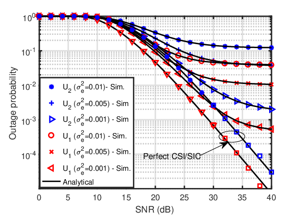
Fig. 3 investigates the impact of CEE σe2\sigma^{2}_{e} on U1U_{1} and U2U_{2} with the fixed residual interference due to SIC error β\beta. It is observed the outage floor decreases with a decrease in σe2\sigma^{2}_{e} and approaches towards perfect CSI/SIC case for both the users. In U1U_{1}, for high CEE values σe2=0.01\sigma^{2}_{e}=0.01 and σe2=0.005\sigma^{2}_{e}=0.005, perfect CSI/SIC has an SNR gain of 4 dB and 3 dB for an outage of 10−110^{-1}. However, for smaller values of CEE (σe2=0.001)(\sigma^{2}_{e}=0.001), the gain is 5 dB for an outage of 10−310^{-3}. Thus, the outage probability is more limited by CEE than SIC error, as high CEE shows degradation in outage probability with the same value of β\beta.

. Refer to caption

Fig. 2: Outage probability of U1U_{1} and U2U_{2} with respect to transmit SNR ( a2=0.7a_{2}=0.7, α=0.35\alpha=0.35).
Refer to caption
Fig. 3: Outage probability of U1U_{1} and U2U_{2} under imperfect CSI/SIC with respect to transmit SNR for different value of σe2\sigma_{e}^{2} ( a2=0.7a_{2}=0.7, α=0.35\alpha=0.35).

Fig. 4 and Fig. 5 illustrate the impact of α\alpha, the fraction of EH time, on the outage probability of U1U_{1} and U2U_{2}. In the given scenario, the α\alpha is ranged between 0.1 and 0.7, whereas the ρ\rho and σe2\sigma_{e}^{2} are fixed at 20 dB and 0.01 respectively. In Fig. 4, the system’s performance comparison under perfect CSI/SIC and imperfect CSI/SIC are shown. With the increase in α\alpha, the EH time increases, thus reducing the information processing time and hence outage probability of users increases for the entire time duration. The plot shows that the optimum value of α\alpha, which minimizes the outage probability, lies in the range of 0.2 to 0.3 for both perfect and imperfect CSI/SIC. Further, it is observed that at a high value of α\alpha, i.e., above 0.45, the outage probability of users become one. With the increase in the α\alpha, the threshold SNR, i.e., γt​h​1\gamma_{th1} and γt​h​2\gamma_{th2}, also increases to maintain the constant target data rates r1r_{1} and r2r_{2}, respectively. Thus, the outage probability criteria γt​h​2<a2a1\gamma_{th2}<\frac{a_{2}}{a_{1}} and γt​h​1<a1β​a2\gamma_{th1}<\frac{a_{1}}{\beta a_{2}} does not satisfied and makes the outage probability Po​u​t,1=Po​u​t,2=1P_{out,1}=P_{out,2}=1. In Fig. 5, the impact of a1a_{1} and β\beta on the outage probability of users under imperfect CSI/SIC is analyzed. In the case of U2U_{2}, it is observed that the outage probability with a1=0.1a_{1}=0.1 shows significant improvement over a1=0.3a_{1}=0.3 since more power is allocated to the symbol intended for U2U_{2}. However, in U1U_{1}, Po​u​t,1P_{out,1} tends to unity due to failure of outage criteria γt​h​1<a1β​a2\gamma_{th1}<\frac{a_{1}}{\beta a_{2}} and γt​h​2<a2a1\gamma_{th2}<\frac{a_{2}}{a_{1}}. Considering the high residual interference due to imperfect SIC, i.e., β=0.16\beta=0.16 and β=0.1\beta=0.1, the outage criteria is not satisfied and leads to constant noise error floor. With a further decrease in residual interference i.e. β=0.01\beta=0.01, the outage probability of U1U_{1} reduces. Hence, selection of a1a_{1} and β\beta plays a crucial role on the outage performance of U1U_{1}.

Refer to caption
Fig. 4: Outage probability of U1U_{1} and U2U_{2} with respect to α\alpha (K=2, ρ=20​d​B\rho=20dB, a2=0.7a_{2}=0.7)
Refer to caption
Fig. 5: Outage probability of U1U_{1} and U2U_{2} under imperfect CSI/SIC with respect to α\alpha (K=2, ρ=20​d​B\rho=20dB, σe2=0.01\sigma_{e}^{2}=0.01)
Refer to caption
Fig. 6: System throughput with respect to transmit SNR, comparison study of optimized and non optimized fraction of EH time (K=2, a1=0.3a_{1}=0.3)
Refer to caption
Fig. 7: Ergidic rate of U1U_{1} and U2U_{2} with respect to transmit SNR (K=2, a1=0.3a_{1}=0.3)

Fig. 6 shows the system throughput under optimized and non-optimized, i.e., (arbitrary) α=0.3\alpha=0.3 value. It is observed that the system throughput of the optimized NOMA scheme under both perfect and imperfect SIC/CSI is enhanced compared to the non-optimized value. It is observed that at the system throughput of 0.3 bps/Hz, the optimized value provides an SNR gain of 3 dB over the non-optimized fixed value. In Fig. 7, both users’ ergodic rate under perfect CSI/SIC and imperfect CSI/SIC are plotted against SNR. It is observed from the figure that the ergodic rate of U1U_{1} under perfect CSI/SIC outperforms the ergodic rate of all other cases. The ergodic rate of U1U_{1} under perfect CSI/SIC increases linearly with the SNR, whereas in case of U2U_{2}, the ergodic rate saturate at a high SNR region. The ergodic rate of 0.5 bps/Hz the U1U_{1} provides an SNR gain of 7 dB over U2U_{2} with perfect CSI/SIC. With the increase in SNR, the interference generated by the symbol of U1U_{1} increases and leads to saturation in the ergodic rate plot. It is also observed that both users under imperfect CSI/SIC shows are marginal increasing trend at low SNR region and saturates at high SNR region. This is due to the increase in SNR, the interference due to imperfect CSI/SIC increases, thus the ergodic rate reduces effectively. Further, the NOMA system’s sum rate (i.e., r1+r2r_{1}+r_{2}) is also presented under perfect CSI/SIC and imperfect CSI/SIC. For the ergodic rate of 1 bps/Hz, the perfect CSI/SIC case provides an SNR gain of 10dB over imperfect CSI/SIC. It is observed that at high SNR values, there is a marginal gap between the analytical and simulated curve for U1U_{1}, which is because of the approximation used in the analytical expression.

VII Conclusion

In this paper, the analysis of downlink multiple EH relay-based NOMA system over Nakagami−m-m fading is performed. The practical assumption of imperfect SIC and imperfect CSI were taken into consideration for investigation. The closed-form expressions for the outage probability, asymptotic outage probability, and ergodic rate of the users under imperfect CSI/SIC are obtained. The analytical results showed that the system under imperfect CSI/SIC provides massive performance degradation compared to the perfect CSI/SIC NOMA system. It is observed that the users’ performance improved with increasing the total number of active relay nodes in the system. The significance of channel estimation error over the performance of users is analyzed. The impact of power allocation coefficient and a fraction of block time over the user performances are also analyzed. Further, the impact of SIC error over the performance of U1U_{1} is analyzed. It is also observed that there is an optimum value of α\alpha for users’ minimum outage probability. Obtained analytical results are validated through extensive simulation results. This generalized analysis is useful for future applications, including UAV, THz, and Internet of Things deployments for beyond 5G networks.

Appendix A Proof of lemma 1

Proof.

The closed-from expression of () is derived as follows. Consider the outage probability definition given in (III-A). Substituting (2), (3), (4) and (5) in (III-A), on rearranging, we get

Po​u​t,1=\displaystyle\small P_{out,1}= 1−Pr{|h^s,r|2>γt​h​2​(Ps​σe2+σ02)(a2−a1​γt​h​2)​Ps,\displaystyle 1-\Pr\Big\{|\hat{h}_{s,r}|^{2}>\frac{\gamma_{th2}(P_{s}\sigma^{2}_{e}+\sigma^{2}_{0})}{(a_{2}-a_{1}\gamma_{th2})P_{s}},
|h^rk,1|2>γt​h​2​(Pr​σe2+σ02)(a2−a1​γt​h​2)​Pr,\displaystyle|\hat{h}_{r_{k},1}|^{2}>\frac{\gamma_{th2}(P_{r}\sigma^{2}_{e}+\sigma^{2}_{0})}{(a_{2}-a_{1}\gamma_{th2})P_{r}},
|h^s,r|2>γt​h​1​(Ps​σe2​(a2+β​a1)+σ02)(a1−β​a2​γt​h​1)​Ps,\displaystyle|\hat{h}_{s,r}|^{2}>\frac{\gamma_{th1}(P_{s}\sigma^{2}_{e}(a_{2}+\beta a_{1})+\sigma^{2}_{0})}{(a_{1}-\beta a_{2}\gamma_{th1})P_{s}},
|h^rk,1|2>γt​h​1​(Pr​σe2​(a1+β​a2)+σ02)(a1−β​a2​γt​h​1)​Pr},\displaystyle|\hat{h}_{r_{k},1}|^{2}>\frac{\gamma_{th1}(P_{r}\sigma^{2}_{e}(a_{1}+\beta a_{2})+\sigma^{2}_{0})}{(a_{1}-\beta a_{2}\gamma_{th1})P_{r}}\Big\}, (A.1)

According to EH criteria the transmitted power at relay is given as Pr=2​Ps​μ​|h^s,r|2​α1−αP_{r}=\frac{2P_{s}\mu|\hat{h}_{s,r}|^{2}\alpha}{1-\alpha}. Substituting PrP_{r} in (A), and after some simplification (A) is given as

Po​u​t,1=\displaystyle\small P_{out,1}= 1−Pr{|h^s,r|2>ψ,|hrk,1|2>λ1|h^s,r|2\displaystyle 1-\Pr\Big\{|\hat{h}_{s,r}|^{2}>\psi,\,|h_{r_{k},1}|^{2}>\frac{\lambda_{1}}{|\hat{h}_{s,r}|^{2}}
+Ω1,|hrk,1|2>λ2|h^s,r|2+Ω2},\displaystyle+\Omega_{1},\,|h_{r_{k},1}|^{2}>\frac{\lambda_{2}}{|\hat{h}_{s,r}|^{2}}+\Omega_{2}\Big\}, (A.2)

where, Δ1=γt​h​2​(σe2+(1/ρ))(a2−a1​γt​h​2)\Delta_{1}=\frac{\gamma_{th2}(\sigma^{2}_{e}+(1/\rho))}{(a_{2}-a_{1}\gamma_{th2})}, λ1=γt​h​2​(1−α)(a2−a1​γt​h​2)​α​μ​2​ρ\lambda_{1}=\frac{\gamma_{th2}\left(1-\alpha\right)}{\left(a_{2}-a_{1}\gamma_{th2}\right)\alpha\mu 2\rho}, λ2=γt​h​1​(1−α)(a1−a2​β​γt​h​1)​α​μ​2​ρ\lambda_{2}=\frac{\gamma_{th1}\left(1-\alpha\right)}{\left(a_{1}-a_{2}\beta\gamma_{th1}\right)\alpha\mu 2\rho}, Ω1=γt​h​2​σe2a2−a1​γt​h​2\Omega_{1}=\frac{\gamma_{th2}\sigma_{e}^{2}}{a_{2}-a_{1}\gamma_{th2}}, Ω2=γt​h​2​(a1+a2​β)​σe2a1−a2​β​γt​h​2\Omega_{2}=\frac{\gamma_{th2}\left(a_{1}+a_{2}\beta\right)\sigma_{e}^{2}}{a_{1}-a_{2}\beta\gamma_{th2}}, ψ=max⁡[Δ1,γt​h​1​(Ps​σe2​(a1+a2​β)+σ02)(a1−a2​β​γt​h​1)​Ps]\psi=\max\left[\Delta_{1},\frac{\gamma_{th1}\left(P_{s}\sigma_{e}^{2}\left(a_{1}+a_{2}\beta\right)+\sigma_{0}^{2}\right)}{\left(a_{1}-a_{2}\beta\gamma_{th1}\right)P_{s}}\right].

Po​u​t,1=\displaystyle\small P_{out,1}= 1−[Pr{|h^s,r|2>ψ,|hrk,1|2>λ1|h^s,r|2\displaystyle 1-\Big[\Pr\Big\{|\hat{h}_{s,r}|^{2}>\psi,\,|h_{r_{k},1}|^{2}>\frac{\lambda_{1}}{|\hat{h}_{s,r}|^{2}}
+Ω1,|h^s,r|2>λ2−λ1Ω1−Ω2}\displaystyle+\Omega_{1},\,|\hat{h}_{s,r}|^{2}>\frac{\lambda_{2}-\lambda_{1}}{\Omega_{1}-\Omega_{2}}\Big\}
+Pr{|h^s,r|2>ψ,|hrk,1|2>λ2|h^s,r|2\displaystyle+\Pr\Big\{|\hat{h}_{s,r}|^{2}>\psi,\,|h_{r_{k},1}|^{2}>\frac{\lambda_{2}}{|\hat{h}_{s,r}|^{2}}
+Ω2,|h^s,r|2<λ2−λ1Ω1−Ω2}].\displaystyle+\Omega_{2},\,|\hat{h}_{s,r}|^{2}<\frac{\lambda_{2}-\lambda_{1}}{\Omega_{1}-\Omega_{2}}\Big\}\Big]. (A.3)

Let Po​u​t,1=1−(A+B)P_{out,1}=1-(A+B), where AA and BB are separately evaluated as follows. Assume the links in the network to be independent, γt​h​1<a1a2​β\gamma_{th1}<\frac{a_{1}}{a_{2}\beta}, γt​h​2<a2a1\gamma_{th2}<\frac{a_{2}}{a_{1}}, λ2>λ1\lambda_{2}>\lambda_{1} and Ω1>Ω2\Omega_{1}>\Omega_{2}. Since i.i.d Nakagami fading is assumed, the channel power gains |h^i,j||\hat{h}_{i,j}| are gamma function. The PDF and CDF [36] of |h^i,j|2|\hat{h}_{i,j}|^{2} with parameter mi,jm_{i,j} and λ^i,j\hat{\lambda}_{i,j} is given as

f|h^i,j|2​(x)=(mi,jλ^i,j)mi,j​xmi,j−1Γ⁡(mi,j)​e−x​mi,jλ^i,j,f_{|\hat{h}_{i,j}|^{2}}(x)=\left(\frac{m_{i,j}}{\hat{\lambda}_{i,j}}\right)^{m_{i,j}}\frac{x^{m_{i,j}-1}}{\Gamma(m_{i,j})}e^{\frac{-xm_{i,j}}{\hat{\lambda}_{i,j}}}, (A.4)
F|h^i,j|2​(x)=1−e−x​mi,jλ^i,j​∑n=0mi,j−11n!​(x​mi,jλ^i,j)n,F_{|\hat{h}_{i,j}|^{2}}(x)=1-e^{\frac{-xm_{i,j}}{\hat{\lambda}_{i,j}}}\sum_{n=0}^{m_{i,j}-1}\frac{1}{n!}\left(\frac{xm_{i,j}}{\hat{\lambda}_{i,j}}\right)^{n}, (A.5)

Let β^i,j=mi,jλ^i,j\hat{\beta}_{i,j}=\frac{m_{i,j}}{\hat{\lambda}_{i,j}}, since PRS with K-relays is performed,the CDF and PDF of the |h^s,r|2|\hat{h}_{s,r}|^{2} is given by

F|h^s,r|2​(x)=[1−e−x​β^s,rk​∑n=0ms,rk−11n!​(x​β^s,rk)n]K,\small F_{|\hat{h}_{s,r}|^{2}}(x)=\left[1-e^{-x\hat{\beta}_{s,r_{k}}}\sum_{n=0}^{m_{s,r_{k}}-1}\frac{1}{n!}\left(x\hat{\beta}_{s,r_{k}}\right)^{n}\right]^{K}, (A.6)
f|h^s,r|2​(x)=\displaystyle\small f_{|\hat{h}_{s,r}|^{2}}(x)= Kβ^s,rkms,rkxms,rk−1(ms,rk−1)!e−x​β^s,rk[1+∑k=1K−1\displaystyle K{\hat{\beta}_{s,r_{k}}}^{m_{s,r_{k}}}\frac{x^{m_{s,r_{k}}-1}}{(m_{s,r_{k}}-1)!}e^{-x\hat{\beta}_{s,r_{k}}}\Bigg[1+\sum_{k=1}^{K-1}
(−1)k​(K−1k)​e−k​x​β^s,rk\displaystyle(-1)^{k}\binom{K-1}{k}e^{-kx\hat{\beta}_{s,r_{k}}}
(∑n=0ms,rk−11n!(xβ^s,rk)n)k],\displaystyle\left(\sum_{n=0}^{m_{s,r_{k}}-1}\frac{1}{n!}\left(x\hat{\beta}_{s,r_{k}}\right)^{n}\right)^{k}\Bigg], (A.7)

By using the Binomial expression for the term (∑n=0ms,rk−11n!​(x​β^s,rk)n)k\tiny\left(\sum_{n=0}^{m_{s,r_{k}}-1}\frac{1}{n!}\left(x\hat{\beta}_{s,r_{k}}\right)^{n}\right)^{k}, the Binomial expansion is given as [18]

=∑i1=0k∑i2=0k−i2⋯∑ims,rk−1=0k−i1⋯ims,rk−2(ki1)(k−i1i2)…\displaystyle=\sum_{i_{1}=0}^{k}\sum_{i_{2}=0}^{k-i_{2}}\dotsm\sum_{i_{m_{s,r_{k}}-1}=0}^{k-i_{1}\cdots i_{m_{s,r_{k}}-2}}\binom{k}{i_{1}}\binom{k-i_{1}}{i_{2}}\ldots
(k−i1−…​ims,rk−2ims,rk−1)​∏r=0ms,rk−2((β^s,rk​x)rr!)ir+1\displaystyle\binom{k-i_{1}-...i_{m_{s,r_{k}}-2}}{i_{m_{s,r_{k}}-1}}\prod_{r=0}^{m_{s,r_{k}}-2}\left(\frac{{(\hat{\beta}_{s,r_{k}}x)}^{r}}{r!}\right)^{i_{r+1}}
(β^s,rkms,rk−1​x(ms,rk−1)!)k−i1−…​ims,rk−1\displaystyle\left(\frac{\hat{\beta}_{s,r_{k}}^{m_{s,r_{k}}-1}x}{(m_{s,r_{k}}-1)!}\right)^{k-i_{1}-...i_{m_{s},{r_{k}}-1}} (A.8)

Substituting (A) in (A), the CDF is obtained. By utilizing the above equation A is obtained as follows

A=\displaystyle A= ∫x=γ∞[1−Frk,1​(λ1x+Ω1)]​fs,rk​(x)​𝑑x,\displaystyle\int_{x=\gamma}^{\infty}\left[1-F_{r_{k},1}\left(\frac{\lambda_{1}}{x}+\Omega_{1}\right)\right]f_{s,r_{k}}(x)dx, (A.9)
A=\displaystyle A= ∫x=γ∞e−β^rk,1​(λ1x+Ω1)​∑n=0mrk,1−1Kn!​β^s,rkms,rk​e−x​β^s,rk\displaystyle\int_{x=\gamma}^{\infty}e^{-\hat{\beta}_{r_{k},1}\left(\frac{\lambda_{1}}{x}+\Omega_{1}\right)}\sum_{n=0}^{m_{r_{k},1}-1}\frac{K}{n!}\hat{\beta}_{s,r_{k}}^{m_{s,r_{k}}}e^{-x\hat{\beta}_{s,r_{k}}}
(β^rk,1(λ1x+Ω1))nxms,rk−1(ms,rk−1)![1+∑k=1K−1\displaystyle\left(\hat{\beta}_{r_{k},1}\left(\frac{\lambda_{1}}{x}+\Omega_{1}\right)\right)^{n}\frac{x^{m_{s,r_{k}}-1}}{(m_{s,r_{k}}-1)!}\Bigg[1+\sum_{k=1}^{K-1}
(−1)k(K−1k)e−k​x​β^s,rk⋃kΞ1,kΞ2,kxi¯]dx,\displaystyle(-1)^{k}\binom{K-1}{k}e^{-kx\hat{\beta}_{s,r_{k}}}\bigcup_{k}\Xi_{1,k}\Xi_{2,k}x^{\bar{i}}\Bigg]dx, (A.10)

where γ=max[ψ,(λ2−λ1Ω1−Ω2)],⋃k=∑i1=0k∑i2=0k−i2⋯∑ims,rk=0k−i1⋯ims,rk−2,Ξ1,k=(ki1)(k−i1i2)…(k−i1−…​ims,rk−2ims,rk−1),Ξ2,k=∏r=0ms,rk−2(β^s,rkrr!)ir+1(β^s,rkms,rk−1(ms,rk−1)!)k−i1−…​ims,rk−1\gamma=\max\left[\psi,\left(\frac{\lambda_{2}-\lambda_{1}}{\Omega_{1}-\Omega_{2}}\right)\right],\,\bigcup_{k}=\sum_{i_{1}=0}^{k}\sum_{i_{2}=0}^{k-i_{2}}\dotsm\sum_{i_{m_{s,r_{k}}=0}}^{k-i_{1}\cdots i_{m_{s,r_{k}}-2}},\,\Xi_{1,k}=\binom{k}{i_{1}}\binom{k-i_{1}}{i_{2}}...\binom{k-i_{1}-...i_{m_{s,r_{k}}-2}}{i_{m_{s,r_{k}}-1}},\,\Xi_{2,k}=\prod_{r=0}^{m_{s,r_{k}}-2}\left(\frac{\hat{\beta}_{s,r_{k}}^{r}}{r!}\right)^{i_{r+1}}\left(\frac{\hat{\beta}_{s,r_{k}}^{m_{s,r_{k}}-1}}{(m_{s,r_{k}}-1)!}\right)^{k-i_{1}-...i_{m_{s},{r_{k}}}-1} and i¯=(ms,rk−1)​(k−i1)−(ms,rk−2)​i2−(ms,rk−3)​i3−…​ims,rk−1\bar{i}=(m_{s,r_{k}}-1)(k-i_{1})-(m_{s,r_{k}}-2)i_{2}-(m_{s,r_{k}}-3)i_{3}-...i_{m_{s,r_{k}}-1}. Using Binomial expansion on (λ1x+Ω1)n\left(\frac{\lambda_{1}}{x}+\Omega_{1}\right)^{n}, the above equation can further simplified as

A=\displaystyle A= e−β^rk,1​Ω1​∑n=0mrk,1−11n!​β^rk,1n​K​β^s,rkms,rk​1(ms,rk−1)!\displaystyle e^{-\hat{\beta}_{r_{k},1}\Omega_{1}}\sum_{n=0}^{m_{r_{k},1}-1}\frac{1}{n!}\hat{\beta}_{r_{k},1}^{n}K\hat{\beta}_{s,r_{k}}^{m_{s,r_{k}}}\frac{1}{(m_{s,r_{k}}-1)!}
∑j=0n(nj)λ1jΩ1n−j[∫x=γ∞xms,rk−j−1e−x​β^s,rk\displaystyle\sum_{j=0}^{n}\binom{n}{j}\lambda_{1}^{j}\Omega_{1}^{n-j}\Bigg[\int_{x=\gamma}^{\infty}x^{m_{s,r_{k}}-j-1}e^{-x\hat{\beta}_{s,r_{k}}}
e−β^rk,1​λ1x​d​x+∑k=1K−1(−1)k​(K−1k)​⋃kΞ1,k​Ξ2,k\displaystyle e^{\frac{-\hat{\beta}_{r_{k},1}\lambda_{1}}{x}}dx+\sum_{k=1}^{K-1}(-1)^{k}\binom{K-1}{k}\bigcup_{k}\Xi_{1,k}\Xi_{2,k}
∫x=γ∞e−x⁡(k+1)​β^s,rkxms,rk−j+i¯−1e−β^rk,1​λ1xdx].\displaystyle\int_{x=\gamma}^{\infty}e^{-x(k+1)\hat{\beta}_{s,r_{k}}}x^{m_{s,r_{k}}-j+\bar{i}-1}e^{\frac{-\hat{\beta}_{r_{k},1}\lambda_{1}}{x}}dx\Bigg]. (A.11)

Now, using Taylor’s series expansion, as e−β^rk,1​λ1x=∑l1=0Nt(−1)l1l1!​(β^rk,1​λ1x)l1e^{\frac{-\hat{\beta}_{r_{k},1}\lambda_{1}}{x}}=\sum_{l_{1}=0}^{N_{t}}\frac{(-1)^{l_{1}}}{l_{1}!}\left(\frac{\hat{\beta}_{r_{k},1}\lambda_{1}}{x}\right)^{l_{1}} where Nt∈{2,3,…​∞}N_{t}\in\{2,3,...\infty\} and using [35, eq. (3.351.4)] the (A) can be simplified. Further, the B is simplified as follows

B=\displaystyle B= ∫x=ψλ2=λ1Ω1−Ω2[1−Frk,1​(λ2x+Ω2)]​fs,r​(x)​𝑑x.\displaystyle\int_{x=\psi}^{\frac{\lambda_{2}=\lambda_{1}}{\Omega_{1}-\Omega_{2}}}\left[1-F_{r_{k},1}\left(\frac{\lambda_{2}}{x}+\Omega_{2}\right)\right]f_{s,r}(x)dx. (A.12)

The (A.12), can be simplified by following the same approach as used in (A.9), the obtained result Po​u​t,1=1−(A+B)P_{out,1}=1-(A+B) is given by (). ∎

Appendix B Proof of lemma 2

Proof.

The closed form expression of (2) is obtained as follows. Substitute (2) and (6) in (9), after some manipulation (9) can be simplified as

Po​u​t,2=\displaystyle P_{out,2}= 1−Pr{|h^s,r|2>γt​h​2​(Ps​σe2+σ02)(a2−a1​γt​h​2)​Ps,\displaystyle 1-\Pr\Big\{|\hat{h}_{s,r}|^{2}>\frac{\gamma_{th2}(P_{s}\sigma^{2}_{e}+\sigma^{2}_{0})}{(a_{2}-a_{1}\gamma_{th2})P_{s}},
|h^rk,2|2>γt​h​2​(Pr​σe2+σ02)(a2−a1​γt​h​2)​Pr},\displaystyle|\hat{h}_{r_{k},2}|^{2}>\frac{\gamma_{th2}(P_{r}\sigma^{2}_{e}+\sigma^{2}_{0})}{(a_{2}-a_{1}\gamma_{th2})P_{r}}\Big\}, (B.1)

Substituting Pr=2​Ps​α​μ​|h^s,r|21−αP_{r}=\frac{2P_{s}\alpha\mu|\hat{h}_{s,r}|^{2}}{1-\alpha}, (B) can be further reduced as

Po​u​t,2=\displaystyle P_{out,2}= 1−Pr{|h^s,r|2>Δ1,\displaystyle 1-\Pr\Big\{|\hat{h}_{s,r}|^{2}>\Delta_{1},
|h^rk,1|2>λ1|h^s,r|2+Ω1},\displaystyle|\hat{h}_{r_{k},1}|^{2}>\frac{\lambda_{1}}{|\hat{h}_{s,r}|^{2}}+\Omega_{1}\Big\}, (B.2)
Po​u​t,2=\displaystyle P_{out,2}= 1−∫x=Δ1∞[1−Frk,2​(λ1x+Ω1)]​fs,r​(x)​𝑑x.\displaystyle 1-\int_{x=\Delta_{1}}^{\infty}\left[1-F_{r_{k},2}\left(\frac{\lambda_{1}}{x}+\Omega_{1}\right)\right]f_{s,r}(x)dx. (B.3)

The integration in (B.3) can be simply simplify by following the same approach as of (A.9) of Appendix A. The obtained closed-form expression is given by (2). ∎

Appendix C Proof of lemma 3

Proof.

Considering the perfect CSI and perfect SIC condition on the SINR’s equation (2), (3), (4) and (5). The outage probability of U1U_{1} under perfect SIC and perfect CSI is given as

Po​u​t,1P=\displaystyle P_{out,1}^{P}= 1−Pr{|hs,r|2​Ps​a2|hs,r|2​Ps​a1+σ02.>γt​h​2,\displaystyle 1-\Pr\Big\{\frac{|{h}_{s,r}|^{2}P_{s}a_{2}}{|{h}_{s,r}|^{2}P_{s}a_{1}+\sigma^{2}_{0}}.>\gamma_{th2},
|hrk,1|2​Pr​a2|hrk,1|2​Pr​a1+σ02>γt​h​2,|hs,r|2​Ps​a1σ02\displaystyle\frac{|{h}_{r_{k},1}|^{2}P_{r}a_{2}}{|{h}_{r_{k},1}|^{2}P_{r}a_{1}+\sigma^{2}_{0}}>\gamma_{th2},\frac{|{h}_{s,r}|^{2}P_{s}a_{1}}{\sigma^{2}_{0}}
>γt​h​1,|hrk,1|2​Pr​a1σ02.>γt​h​1}.\displaystyle>\gamma_{th1},\frac{|{h}_{r_{k},1}|^{2}P_{r}a_{1}}{\sigma^{2}_{0}}.>\gamma_{th1}\Big\}. (C.1)

substituting Pr=2​Ps​μ​|hs,r|2​α1−αP_{r}=\frac{2P_{s}\mu|h_{s,r}|^{2}\alpha}{1-\alpha} and after some manipulation, (C) further simplified as

Po​u​t,1P=\displaystyle P_{out,1}^{P}= 1−Pr⁡{|hs,r|2>Δ3,|hrk,1|>Δ2|hs,r|2},\displaystyle 1-\Pr\Big\{|{h}_{s,r}|^{2}>\Delta_{3},|{h}_{r_{k},1}|>\frac{\Delta_{2}}{|h_{s,r}|^{2}}\Big\}, (C.2)

where Δ3=max⁡[γt​h​2​σ02(a2−a1​γt​h​2)​Ps,γt​h​1​σ02a1​Ps]\Delta_{3}=\max[\frac{\gamma_{th2}\sigma_{0}^{2}}{(a_{2}-a_{1}\gamma_{th2})P_{s}},\frac{\gamma_{th1}\sigma_{0}^{2}}{a_{1}P_{s}}], Δ2=max⁡[λ1,γt​h​1​(1−α)a1​α​2​μ​Ps]\Delta_{2}=\max[\lambda_{1},\frac{\gamma_{th1}(1-\alpha)}{a_{1}\alpha 2\mu P_{s}}]. Let Po​u​t,1P=1−DP_{out,1}^{P}=1-D, where D is evaluated as follow

D=\displaystyle D= ∫x=Δ3∞[1−Frk,1​(Δ2x)]​fs,rk​(x)​𝑑x,\displaystyle\int_{x=\Delta_{3}}^{\infty}\left[1-F_{r_{k},1}\left(\frac{\Delta_{2}}{x}\right)\right]f_{s,r_{k}}(x)dx, (C.3)
=\displaystyle= ∑n=0mrk,1−11(ms,rk−1)!​(mrk,1​Δ2λrk,1)n​(ms,rkλs,rk)ms,rk\displaystyle\sum_{n=0}^{m_{r_{k},1}-1}\frac{1}{(m_{s,r_{k}}-1)!}\left(\frac{m_{r_{k},1}\Delta_{2}}{\lambda_{r_{k},1}}\right)^{n}\left(\frac{m_{s,r_{k}}}{\lambda_{s,r_{k}}}\right)^{m_{s,r_{k}}}
Kn![∫x=Δ3∞xms,rk−n−1ems,rk​xλs,rke−mrk,1​Δ2λrk,1​xdx\displaystyle\frac{K}{n!}\Bigg[\int_{x=\Delta_{3}}^{\infty}x^{m_{s,r_{k}}-n-1}e^{\frac{m_{s,r_{k}}x}{\lambda_{s,r_{k}}}}e^{\frac{-m_{r_{k},1}\Delta_{2}}{\lambda_{r_{k},1}x}}dx
+∑k=1K−1(−1)k(K−1k)⋃kΞ1,kΞ2,k∫x=Δ3∞\displaystyle+\sum_{k=1}^{K-1}(-1)^{k}\binom{K-1}{k}\bigcup_{k}\Xi_{1,k}\Xi_{2,k}\int_{x=\Delta_{3}}^{\infty}
e−x⁡(k+1)​ms,rkλs,rkxms,rk−n+i¯−1e−mrk,1​Δ2λrk,1​xdx].\displaystyle e^{\frac{-x(k+1)m_{s,r_{k}}}{\lambda_{s,r_{k}}}}x^{m_{s,r_{k}}-n+\bar{i}-1}e^{\frac{-m_{r_{k},1}\Delta_{2}}{\lambda_{r_{k},1}x}}dx\Bigg].

The integration in (C), is same as in (A) in appendix A. Hence, D can be obtained following the similar procedure as adopted in (A), which is given by (3). ∎

References

  • [1] Z. Ding, X. Lei, G. K. Karagiannidis, R. Schober, J. Yuan, and V. K. Bhargava, “A survey on non-orthogonal multiple access for 5G networks: Research challenges and future trends,” IEEE J. Sel. Areas Commun., vol. 35, no. 10, pp. 2181–2195, Jul. 2017.
  • [2] P. Swami, V. Bhatia, S. Vuppala, and T. Ratnarajah, “A cooperation scheme for user fairness and performance enhancement in NOMA-HCN,” IEEE Trans. Veh. Technol., vol. 67, no. 12, pp. 11 965–11 978, Oct. 2018.
  • [3] Y. Liu, Z. Qin, M. Elkashlan, Z. Ding, A. Nallanathan, and L. Hanzo, “Nonorthogonal Multiple Access for 5G and Beyond,” IEEE Proc., vol. 105, no. 12, pp. 2347–2381, Dec. 2017.
  • [4] J. Kim and I. Lee, “Non-Orthogonal Multiple Access in Coordinated Direct and Relay Transmission,” IEEE Commun. Lett., vol. 19, no. 11, pp. 2037–2040, Nov. 2015.
  • [5] Z. Ding, M. Peng, and H. V. Poor, “Cooperative non-orthogonal multiple access in 5G systems,” IEEE Commun. Lett., vol. 19, no. 8, pp. 1462–1465, Jun. 2015.
  • [6] J. Men, J. Ge, and C. Zhang, “Performance analysis of nonorthogonal multiple access for relaying networks over Nakagami-mm fading channels,” IEEE Trans. Veh. Technol., vol. 66, no. 2, pp. 1200–1208, Feb. 2017.
  • [7] Z. Ding, H. Dai, and H. V. Poor, “Relay selection for cooperative NOMA,” IEEE Wireless Commun. Lett., vol. 5, no. 4, pp. 416–419, Aug. 2016.
  • [8] P. Xu, Z. Yang, Z. Ding, and Z. Zhang, “Optimal relay selection schemes for cooperative NOMA,” IEEE Trans. on Veh. Technol., vol. 67, no. 8, pp. 7851–7855, Aug. 2018.
  • [9] Y. Li, Y. Li, X. Chu, Y. Ye, and H. Zhang, “Performance analysis of relay selection in cooperative NOMA networks,” IEEE Commun. Lett., vol. 23, no. 4, pp. 760–763, Apr. 2019.
  • [10] S. Lee, D. B. da Costa, Q. Vien, T. Q. Duong, and R. T. de Sousa, “Non-orthogonal multiple access schemes with partial relay selection,” IET Commun., vol. 11, no. 6, pp. 846–854, Apr. 2017.
  • [11] J. Jose, P. Shaik, and V. Bhatia, “VFD-NOMA under imperfect SIC and residual inter-relay interference over generalized nakagami-m fading channels,” IEEE Commun. Lett., pp. 1–1, 2020.
  • [12] Y. Liu, Z. Ding, M. Elkashlan, and H. V. Poor, “Cooperative non-orthogonal multiple access with simultaneous wireless information and power transfer,” IEEE J. Sel. Areas Commun., vol. 34, no. 4, pp. 938–953, Apr. 2016.
  • [13] H. Dac-Binh and N. Sang Quang, “Outage performance of energy harvesting DF relaying NOMA networks,” Mobile Netw. and Appl., vol. 23, no. 6, pp. 1572–1585, Dec. 2018.
  • [14] Y. Zhang and J. Ge, “Performance analysis for non-orthogonal multiple access in energy harvesting relaying networks,” IET Commun., vol. 11, no. 11, pp. 1768–1774, Aug. 2017.
  • [15] H.  Tran Manh, N. Tan. Nguyen Trungand Hoang, and P. Hiep, “Performance analysis of decode-and-forward partial relay selection in NOMA systems with RF energy harvesting,” Wireless Netw., vol. 25, no. 8, pp. 4585–4595, Feb. 2019.
  • [16] X. Li, J. Li, P. T. Mathiopoulos, D. Zhang, L. Li, and J. Jin, “Joint impact of hardware impairments and imperfect CSI on cooperative SWIPT NOMA multi-relaying systems,” Proc. IEEE/CIC Int. Conf. commun. China, pp. 95–99, Jul. 2018.
  • [17] D. Do, M. Vaezi, and T. Nguyen, “Wireless powered cooperative relaying using NOMA with imperfect CSI,” in Proc. IEEE Globecom Workshops, Dec. 2018, pp. 1–6.
  • [18] J. Men, J. Ge, and C. Zhang, “Performance analysis for downlink relaying aided non-orthogonal multiple access networks with imperfect CSI over Nakagami-m{m} fading,” IEEE Access, vol. 5, pp. 998–1004, Mar. 2017.
  • [19] P. Shaik, P. K. Singya, and V. Bhatia, “On impact of imperfect CSI over hexagonal QAM for TAS/MRC-MIMO cooperative relay network,” IEEE Commun. Lett., vol. 23, no. 10, pp. 1721–1724, Oct. 2019.
  • [20] E. N. Papasotiriou, A. A. Boulogeorgos, and A. Alexiou, “Performance analysis of THz wireless systems in the presence of antenna misalignment and phase noise,” IEEE Commun. Lett., vol. 24, no. 6, pp. 1211–1215, Jun. 2020.
  • [21] M. Alzenad and H. Yanikomeroglu, “Coverage and rate analysis for unmanned aerial vehicle base stations with LoS/NLoS propagation,” in Proc. IEEE Globecom Commun. Conf. Workshops, Dec. 2018, pp. 1–7.
  • [22] S. M. Kay, Fundamental of statistical signal processing: estimation theory. Prentice-hall, 1993.
  • [23] X. Liang, Y. Wu, D. W. K. Ng, S. Jin, Y. Yao, and T. Hong, “Outage probability of cooperative NOMA networks under imperfect CSI with user selection,” IEEE Access, vol. 8, pp. 117 921–117 931, May 2020.
  • [24] D. Do, T. Anh Le, T. N. Nguyen, X. Li, and K. M. Rabie, “Joint impacts of imperfect CSI and imperfect SIC in cognitive radio-assisted NOMA-V2X communications,” IEEE Access, vol. 8, pp. 128 629–128 645, Jul. 2020.
  • [25] Taesang Yoo and A. Goldsmith, “Capacity and power allocation for fading MIMO channels with channel estimation error,” IEEE Trans. on Inf. Theory, vol. 52, no. 5, pp. 2203–2214, May 2006.
  • [26] F. Fang, H. Zhang, J. Cheng, S. Roy, and V. C. M. Leung, “Joint user scheduling and power allocation optimization for energy-efficient noma systems with imperfect CSI,” IEEE J. Sel. Areas in Commun., vol. 35, no. 12, pp. 2874–2885, Dec. 2017.
  • [27] L. L. Scharf, Statistical Signal Processing: Detection, Estimation, and Time-series Analysis. Reading, MA: Addison-Wesley, 1991.
  • [28] I. Krikidis, J. Thompson, S. Mclaughlin, and N. Goertz, “Amplify-and-forward with partial relay selection,” IEEE Commun. Lett., vol. 12, no. 4, pp. 235–237, Apr. 2008.
  • [29] S. Parvez, D. Kumar, and V. Bhatia, “On performance of SWIPT enabled two-way relay system with non-linear power amplifier,” in National Conf. on Commun., Feb. 2020, pp. 1–6.
  • [30] S. Parvez, P. K. Singya, and V. Bhatia, “On ASER analysis of energy efficient modulation schemes for a device-to-device MIMO relay network,” IEEE Access, vol. 8, pp. 2499–2512, Jan. 2020.
  • [31] P. Shaik, P. K. Singya, N. Kumar, K. K. Garg, and V. Bhatia, “On impact of imperfect CSI over SWIPT device-to-device (D2D) MIMO relay systems,” in 2020 Int. Conf. on Signal Process. and Commun., 2020, pp. 1–5.
  • [32] W. Shuming, Z. Yudong, W. Shuihua, and J. Genlin, “A comprehensive survey on particle swarm optimization algorithm and its applications,” Math. Problems Eng., pp. 1211–1215, Feb. 2015.
  • [33] M. Song and M. Zheng, “Energy efficiency optimization for wireless powered sensor networks with nonorthogonal multiple access,” IEEE Sensors Lett., vol. 2, no. 1, pp. 1–4, Mar. 2018.
  • [34] A. Masaracchia, D. B. Da Costa, T. Q. Duong, M. Nguyen, and M. T. Nguyen, “A PSO-based approach for user-pairing schemes in NOMA systems: Theory and applications,” IEEE Access, vol. 7, pp. 90 550–90 564, Jul. 2019.
  • [35] I. S. Gradshteyn and I. M. Ryzhik, Table of integrals, series, and products. Academic Press, 2014.
  • [36] A. Goldsmith, Wireless Communications. Cambridge University Press, 2005.