跳到论文正文
W Papers独立论文阅读器 arXiv:2105.06884 论文正文 计算阅读时间 · 0%
引用这篇论文根据当前论文元数据生成,正式投稿前建议核对。


License: arXiv.org perpetual non-exclusive license
arXiv:2105.06884v3 [math.ST] 19 Apr 2022

Nadaraya-Watson Estimator for I.I.D. Paths of Diffusion Processes

Nicolas MARIE† Address: †,⋄Laboratoire Modal’X, Université Paris Nanterre, Nanterre, France Email address: nmarie@parisnanterre.fr and Amélie ROSIER⋄ Address: ⋄ESME Sudria, Paris, France Email address: amelie.rosier@esme.fr
Abstract.

This paper deals with a nonparametric Nadaraya-Watson estimator b^\widehat{b} of the drift function computed from independent continuous observations of a diffusion process. Risk bounds on b^\widehat{b} and its discrete-time approximation are established. The paper also deals with extensions of the PCO and leave-one-out cross validation bandwidth selection methods for b^\widehat{b}. Finally, some numerical experiments are provided.

Key words and phrases: 
Diffusion processes ; Nonparametric drift estimation ; Nadaraya-Watson estimator ; PCO method ; Cross validation.

MSC2020 subject classifications. 62G05 ; 62M05.

1. Introduction

Consider the stochastic differential equation

(1) Xt=x0+∫0tb⁡(Xs)​𝑑s+∫0tσ⁡(Xs)​d​Ws,X_{t}=x_{0}+\int_{0}^{t}b(X_{s})ds+\int_{0}^{t}\sigma(X_{s})dW_{s},

where b,σ:ℝ→ℝb,\sigma:\mathbb{R}\rightarrow\mathbb{R} are two continuous functions and W=(Wt)t∈[0,T]W=(W_{t})_{t\in[0,T]} is a Brownian motion.

Since the 1980’s, the statistical inference for stochastic differential equations (SDE) has been widely investigated by many authors in the parametric and in the nonparametric frameworks. Classically (see Hoffmann [20], Kessler [22], Kutoyants [24], Dalalyan [9], Comte et al. [6], etc.), the estimators of the drift function are computed from one path of the solution to Equation (1) and converge when TT goes to infinity. The existence and the uniqueness of the stationary solution to Equation (1) are then required, and obtained thanks to restrictive conditions on bb.

Let ℐ:(x,w)↦ℐ⁡(x,w)\mathcal{I}:(x,w)\mapsto\mathcal{I}(x,w) be the Itô map for Equation (1) and, for N∈ℕ∗N\in\mathbb{N}^{*} copies W1,…,WNW^{1},\dots,W^{N} of WW, consider Xi=ℐ⁡(x0,Wi)X^{i}=\mathcal{I}(x_{0},W^{i}) for every i∈{1,…,N}i\in\{1,\dots,N\}. The estimation of the drift function bb from continuous-time and discrete-time observations of (X1,…,XN)(X^{1},\dots,X^{N}) is a functional data analysis problem already investigated in the parametric framework (see Ditlevsen and De Gaetano [16], Overgaard et al. [27], Picchini, De Gaetano and Ditlevsen [28], Picchini and Ditlevsen [29], Comte, Genon-Catalot and Samson [7], Delattre and Lavielle [12], Delattre, Genon-Catalot and Samson [11], Dion and Genon-Catalot [15], Delattre, Genon-Catalot and Larédo [10], etc.) and more recently in the nonparametric framework (see Comte and Genon-Catalot [4, 5], Della Maestra and Hoffmann [13] and Denis et al. [14]). In [13], the authors also study a Nadaraya-Watson type estimator, presented bellow, of the drift function in McKean-Vlasov models.

Under the appropriate conditions on bb and σ\sigma recalled at Section 2, the distribution of XtX_{t} has a density pt(x0,.)p_{t}(x_{0},.) for every t∈(0,T]t\in(0,T], and then one can define

f⁡(x):=1T−t0​∫t0Tpt​(x0,x)​𝑑t​ ; ​x∈ℝf(x):=\frac{1}{T-t_{0}}\int_{t_{0}}^{T}p_{t}(x_{0},x)dt\textrm{ $;$ }x\in\mathbb{R}

for any t0>0t_{0}>0. Clearly, ff is a density function:

∫−∞∞f⁡(x)​𝑑x=1T−t0​∫t0T∫−∞∞pt​(x0,x)​𝑑x​𝑑t=1.\int_{-\infty}^{\infty}f(x)dx=\frac{1}{T-t_{0}}\int_{t_{0}}^{T}\int_{-\infty}^{\infty}p_{t}(x_{0},x)dxdt=1.

Let K:ℝ→ℝK:\mathbb{R}\rightarrow\mathbb{R} be a kernel (i.e. an integrable function such that ∫K=1\int K=1) and consider Kh​(x):=h−1​K​(h−1​x)K_{h}(x):=h^{-1}K(h^{-1}x) with h∈(0,1]h\in(0,1]. In the spirit of Comte and Genon-Catalot [4, 5], our paper deals first with the continuous-time Nadaraya-Watson estimator

(2) b^N,h​(x):=b​f^N,h​(x)f^N,h​(x)\widehat{b}_{N,h}(x):=\frac{\widehat{bf}_{N,h}(x)}{\widehat{f}_{N,h}(x)}

of the drift function bb, where

(3) f^N,h​(x):=1N⁡(T−t0)​∑i=1N∫t0TKh​(Xti−x)​𝑑t\widehat{f}_{N,h}(x):=\frac{1}{N(T-t_{0})}\sum_{i=1}^{N}\int_{t_{0}}^{T}K_{h}(X_{t}^{i}-x)dt

is an estimator of ff and

(4) b​f^N,h​(x):=1N⁡(T−t0)​∑i=1N∫t0TKh​(Xti−x)​d​Xti\widehat{bf}_{N,h}(x):=\frac{1}{N(T-t_{0})}\sum_{i=1}^{N}\int_{t_{0}}^{T}K_{h}(X_{t}^{i}-x)dX_{t}^{i}

is an estimator of b​fbf. From independent copies of XX continuously observed on [0,T][0,T], b^N,h\widehat{b}_{N,h} is a natural extension of the Nadaraya-Watson estimator already well-studied in the regression framework (see Comte [2], Chapter 4 or Györfi et al. [18], Chapter 5). The paper also deals with a discrete-time approximate of the previous Nadaraya-Watson estimator:

(5) b^n,N,h​(x):=b​f^n,N,h​(x)f^n,N,h​(x),\widehat{b}_{n,N,h}(x):=\frac{\widehat{bf}_{n,N,h}(x)}{\widehat{f}_{n,N,h}(x)},

where

(6) f^n,N,h​(x):=1n​N​∑i=1N∑j=0n−1Kh​(Xtji−x)\widehat{f}_{n,N,h}(x):=\frac{1}{nN}\sum_{i=1}^{N}\sum_{j=0}^{n-1}K_{h}(X_{t_{j}}^{i}-x)

is an estimator of ff,

(7) b​f^n,N,h​(x):=1N⁡(T−t0)​∑i=1N∑j=0n−1Kh​(Xtji−x)​(Xtj+1i−Xtji)\widehat{bf}_{n,N,h}(x):=\frac{1}{N(T-t_{0})}\sum_{i=1}^{N}\sum_{j=0}^{n-1}K_{h}(X_{t_{j}}^{i}-x)(X_{t_{j+1}}^{i}-X_{t_{j}}^{i})

is an estimator of b​fbf, and (t0,t1,…,tn)(t_{0},t_{1},\dots,t_{n}) is the dissection of [t0,T][t_{0},T] such that tj=t0+(T−t0)​j/nt_{j}=t_{0}+(T-t_{0})j/n for every j∈{1,…,n}j\in\{1,\dots,n\}. Finally, our paper deals with a risk bound on the adaptive double bandwidths Nadaraya-Watson’s estimator

b^N,h^,h^′​(x):=b​f^N,h^​(x)f^N,h^′​(x),\widehat{b}_{N,\widehat{h},\widehat{h}^{\prime}}(x):=\frac{\widehat{bf}_{N,\widehat{h}}(x)}{\widehat{f}_{N,\widehat{h}^{\prime}}(x)},

where h^\widehat{h} (resp. h^′\widehat{h}^{\prime}) is selected via a penalized comparison to overfitting (PCO) type criterion for its numerator (resp. denominator). However, in the nonparametric regression framework, it is established in Comte and Marie [8] that the leave-one-out cross-validation (looCV) bandwidth selection method for Nadaraya-Watson’s estimator is numerically more satisfactory than two alternative procedures based on Goldenshluger-Lepski’s method and on the PCO method. For this reason, an extension of the looCV method to b^n,N,h\widehat{b}_{n,N,h} is also provided, with numerical experiments, even if it seems difficult to establish a risk bound on the associated adaptive estimator.

Now, let us compare b^N,h\widehat{b}_{N,h} with the estimator of Della Maestra and Hoffmann [13] restricted to our framework:

b^N,𝐡​(x):=∑i=1N∫0TLh1​(τ−t)​Kh2​(Xti−x)​d​Xti∑i=1NKh3​(Xτi−x),\widehat{b}_{N,\mathbf{h}}(x):=\frac{\displaystyle{\sum_{i=1}^{N}\int_{0}^{T}L_{h_{1}}(\tau-t)K_{h_{2}}(X_{t}^{i}-x)dX_{t}^{i}}}{\displaystyle{\sum_{i=1}^{N}K_{h_{3}}(X_{\tau}^{i}-x)}},

where L:ℝ→ℝL:\mathbb{R}\rightarrow\mathbb{R} is another kernel, h1,h2,h3∈(0,1]h_{1},h_{2},h_{3}\in(0,1], 𝐡=(h1,h2,h3)\mathbf{h}=(h_{1},h_{2},h_{3}) and τ∈(0,T)\tau\in(0,T). In [13], the authors provide a nice risk bound on the adaptive estimator obtained by selecting (h1,h2)(h_{1},h_{2}) (resp. h3h_{3}) via a Goldenshluger-Lepski type procedure on the numerator (resp. the denominator) of b^N,𝐡\widehat{b}_{N,\mathbf{h}}. As mentioned above, in Comte and Marie [8], it has been established that in the nonparametric regression framework, this approach is numerically less satisfactory than the looCV method. However, the looCV method provided in our paper doesn’t extend to b^N,𝐡\widehat{b}_{N,\mathbf{h}} because it cannot be written easily as a linear combination. Note also that even if it is numerically less satisfactory than the looCV method provided at Subsection 5.2, the PCO type method provided in our paper at Subsection 5.1 is easier to implement and numerically faster than a Goldenshluger-Lepski type method because, as in the nonparametric regression framework, the criterion to minimize depends on one variable instead of two, and because there is no constant to calibrate. For technical reasons explained at Section 6, the condition (N​h3)−1⩽1(Nh^{3})^{-1}\leqslant 1 is required on the bandwidths collection to establish a risk bound on our PCO based adaptive estimator of b​fbf, when Della Maestra and Hoffmann only need the condition log⁡(N)2​(N​h)−1⩽1\log(N)^{2}(Nh)^{-1}\leqslant 1 to establish a risk bound on their Goldenshluger-Lepski based adaptive estimator of bpτ(x0,.)bp_{\tau}(x_{0},.) in [13]. However, Remark 5.4 explains why the condition (N​h3)−1⩽1(Nh^{3})^{-1}\leqslant 1 on the bandwidths collection is not that uncomfortable. Finally, under similar conditions on bb, σ\sigma and KK, the rate of convergence of our continuous-time Nadaraya-Watson estimator is of same order than the rate of convergence of the estimator of Della Maestra and Hoffmann [13] in the nonadaptive case. There is no discrete-time approximate of b^N,𝐡\widehat{b}_{N,\mathbf{h}} studied in [13].

Finally, even if they deal with a different type of nonparametric estimators, let us say few words on the recent papers of Comte and Genon-Catalot [4] and Denis et al. [14]. On the one hand, in [4], the authors extend to the diffusion processes framework, for continuous-time observations, the least squares projection estimator already well studied in the regression framework (see Cohen et al. [1], Comte and Genon-Catalot [3], etc.). In particular, they provide a model selection procedure and establish a risk bound on the associated adaptive estimator. As explained at Section 3, in the nonadaptive case, the variance term of their estimator is comparable with the variance term of b^N,h\widehat{b}_{N,h}, but as in the nonparametric regression framework, the rate of convergence of the least squares projection estimator depends on the regularity space associated to the projection basis. On the other hand, in [14], the authors focus on a projection least squares estimator computed from discrete-time observations and on a BB-spline space. They provide a model selection procedure and prove both upper and lower bounds on the associated adaptive estimator.

Section 2 deals with the existence and the regularity of the density pt(x0,.)p_{t}(x_{0},.) of XtX_{t} for every t∈(0,T]t\in(0,T], and with a Nikol’skii type condition fulfilled by ff. Section 3 deals with a risk bound on the continuous-time Nadaraya-Watson estimator and Section 4 with a risk bound on its discrete-time approximate. Finally, Section 5 provides extensions of the PCO and looCV methods for the Nadaraya-Watson estimator studied in this paper. Some numerical experiments on the looCV based adaptive Nadaraya-Watson estimator are also provided. The proofs are postponed to Appendix A.

Notations and basic definitions:

  • •

    For every A,B∈ℝA,B\in\mathbb{R} such that A<BA<B, C0​([A,B],ℝ)C^{0}([A,B];\mathbb{R}) is equipped with the uniform norm ∥.∥∞,A,B\|.\|_{\infty,A,B}, and C0​(ℝ)C^{0}(\mathbb{R}) is equipped with the uniform (semi-)norm ∥.∥∞\|.\|_{\infty}.

  • •

    For every p∈ℕ¯p\in\overline{\mathbb{N}}, Cbp(ℝ):=∩j=0p{φ∈Cp(ℝ):φ(j) is bounded}C_{\rm b}^{p}(\mathbb{R}):=\cap_{j=0}^{p}\{\varphi\in C^{p}(\mathbb{R}):\varphi^{(j)}\textrm{ is bounded}\}.

  • •

    For every p⩾1p\geqslant 1, 𝕃p​(ℝ,d​x)\mathbb{L}^{p}(\mathbb{R},dx) is equipped with its usual norm ∥.∥p\|.\|_{p} such that

    ‖φ‖p:=(∫−∞∞φ​(x)p​𝑑x)1/p​; ​∀φ∈𝕃p​(ℝ,𝑑x).\|\varphi\|_{p}:=\left(\int_{-\infty}^{\infty}\varphi(x)^{p}dx\right)^{1/p}\textrm{$;$ }\forall\varphi\in\mathbb{L}^{p}(\mathbb{R},dx).
  • •

    ℍ2\mathbb{H}^{2} is the space of the processes (Yt)t∈[0,T](Y_{t})_{t\in[0,T]}, adapted to the filtration generated by WW, such that

    ∫0T𝔼⁡(Yt2)​𝑑t<∞.\int_{0}^{T}\mathbb{E}(Y_{t}^{2})dt<\infty.
  • •

    For a given kernel δ\delta, the usual scalar product on 𝕃2​(ℝ,δ​(x)​d​x)\mathbb{L}^{2}(\mathbb{R},\delta(x)dx) is denoted by ⟨.,.⟩2,δ\langle.,.\rangle_{2,\delta} and the associated norm by ∥.∥2,δ\|.\|_{2,\delta}.

2. Preliminaries: regularity of the density and estimates

This section deals with the existence and the regularity of the density pt(x0,.)p_{t}(x_{0},.) of XtX_{t} for every t∈(0,T]t\in(0,T], with the Kusuoka-Stroock bounds on (t,x)↦pt​(x0,x)(t,x)\mapsto p_{t}(x_{0},x) and its derivatives, and then with a Nikol’skii type condition fulfilled by ff.

In the sequel, in order to ensure the existence and the uniqueness of the (strong) solution to Equation (1), bb and σ\sigma fulfill the following regularity assumption.

Assumption 2.1.

The functions bb and σ\sigma are Lipschitz continuous.

Now, assume that the solution XX to Equation (1) fulfills the following assumption.

Assumption 2.2.

There exists β∈ℕ∗\beta\in\mathbb{N}^{*} such that, for any t∈(0,T]t\in(0,T], the distribution of XtX_{t} has a β\beta times continuously derivable density pt(x0,.)p_{t}(x_{0},.). Moreover, for every x∈ℝx\in\mathbb{R},

0<pt​(x0,x)⩽𝔠2.2,1t1/2​exp⁡[−𝔪2.2,1​(x−x0)2t]0<p_{t}(x_{0},x)\leqslant\frac{\mathfrak{c}_{\ref{assumption_bound_derivative_density_x},1}}{t^{1/2}}\exp\left[-\mathfrak{m}_{\ref{assumption_bound_derivative_density_x},1}\frac{(x-x_{0})^{2}}{t}\right]

and

|∂xℓpt​(x0,x)|⩽𝔠2.2,2​(ℓ)tq2​(ℓ)​exp⁡[−𝔪2.2,2​(ℓ)​(x−x0)2t]​ ; ​∀ℓ∈{1,…,β},|\partial_{x}^{\ell}p_{t}(x_{0},x)|\leqslant\frac{\mathfrak{c}_{\ref{assumption_bound_derivative_density_x},2}(\ell)}{t^{q_{2}(\ell)}}\exp\left[-\mathfrak{m}_{\ref{assumption_bound_derivative_density_x},2}(\ell)\frac{(x-x_{0})^{2}}{t}\right]\textrm{ $;$ }\forall\ell\in\{1,\dots,\beta\},

where all the constants are positive, depend on TT, but not on tt and xx.

At Section 4, the following assumption on XX is also required.

Assumption 2.3.

For any x∈ℝx\in\mathbb{R}, the function t∈(0,T]↦pt​(x0,x)t\in(0,T]\mapsto p_{t}(x_{0},x) is continuously derivable. Moreover,

|∂tpt​(x0,x)|⩽𝔠2.3,3tq3​exp⁡[−𝔪2.3,3​(x−x0)2t]​ ; ​∀t∈(0,T],|\partial_{t}p_{t}(x_{0},x)|\leqslant\frac{\mathfrak{c}_{\ref{assumption_bound_derivative_density_t},3}}{t^{q_{3}}}\exp\left[-\mathfrak{m}_{\ref{assumption_bound_derivative_density_t},3}\frac{(x-x_{0})^{2}}{t}\right]\textrm{ $;$ }\forall t\in(0,T],

where 𝔠2.3,3\mathfrak{c}_{\ref{assumption_bound_derivative_density_t},3}, 𝔪2.3,3\mathfrak{m}_{\ref{assumption_bound_derivative_density_t},3} and q3q_{3} are three positive constants depending on TT but not on tt and xx.

Let us provide some examples of diffusion processes categories satisfying Assumptions 2.2 and/or 2.3.

Examples:

  1. (1)

    Assume that the functions bb and σ\sigma belong to Cb∞​(ℝ)C_{\rm b}^{\infty}(\mathbb{R}), and that there exists α>0\alpha>0 such that

    (8) |σ⁡(x)|>α​ ; ​∀x∈ℝ.|\sigma(x)|>\alpha\textrm{ $;$ }\forall x\in\mathbb{R}.

    Then, by Kusuoka and Stroock [23], Corollary 3.25, XX fulfills Assumptions 2.2 and 2.3.

  2. (2)

    Assume that bb is Lipschitz continuous (but not bounded) and that σ∈Cb1​(ℝ)\sigma\in C_{\rm b}^{1}(\mathbb{R}). Assume also that σ\sigma satisfies the non-degeneracy condition (8) and that σ′\sigma^{\prime} is Hölder continuous. Then, by Menozzi et al. [26], Theorem 1.2, XX fulfills Assumption 2.2 with β=1\beta=1 (but not necessarily Assumption 2.3). Note that the conditions required to apply Menozzi et al. [26], Theorem 1.2 are fulfilled by the so-called Ornstein-Uhlenbeck process, that is the solution to the Langevin equation:

    (9) Xt=x0−θ​∫0tXs​𝑑s+σ​Wt​ ; ​t∈ℝ+,X_{t}=x_{0}-\theta\int_{0}^{t}X_{s}ds+\sigma W_{t}\textrm{ $;$ }t\in\mathbb{R}_{+},

    where θ,σ>0\theta,\sigma>0 and x0∈ℝ+x_{0}\in\mathbb{R}_{+}. In this special case, since it is well-known that the solution to Equation (9) is a Gaussian process such that

    𝔼⁡(Xt)=x0​e−θ​tandvar⁡(Xt)=σ22​θ​(1−e−2​θ​t)​ ; ​∀t∈[0,T],\mathbb{E}(X_{t})=x_{0}e^{-\theta t}\quad\textrm{and}\quad{\rm var}(X_{t})=\frac{\sigma^{2}}{2\theta}(1-e^{-2\theta t})\textrm{ $;$ }\forall t\in[0,T],

    one can show that XX also fulfills Assumption 2.3.

Remark 2.4.

Under Assumptions 2.1 and 2.2, for any p⩾1p\geqslant 1 and any continuous function φ:ℝ→ℝ\varphi:\mathbb{R}\rightarrow\mathbb{R} having polynomial growth, t∈[0,T]↦𝔼⁡(|φ⁡(Xt)|p)t\in[0,T]\mapsto\mathbb{E}(|\varphi(X_{t})|^{p}) is bounded. Indeed, for any t∈[0,T]t\in[0,T],

𝔼⁡(|φ⁡(Xt)|p)\displaystyle\mathbb{E}(|\varphi(X_{t})|^{p}) ⩽\displaystyle\leqslant 𝔠1​(1+𝔼⁡(|Xt|p​q))=𝔠1​∫−∞∞(1+|x|p​q)​pt​(x0,x)​𝑑x\displaystyle\mathfrak{c}_{1}(1+\mathbb{E}(|X_{t}|^{pq}))=\mathfrak{c}_{1}\int_{-\infty}^{\infty}(1+|x|^{pq})p_{t}(x_{0},x)dx
⩽\displaystyle\leqslant 𝔠1​𝔠2.2,1​∫−∞∞(1+|t1/2​x+x0|p​q)​e−𝔪2.2,1​x2​𝑑x⩽𝔠2​(1∨Tp​q/2)\displaystyle\mathfrak{c}_{1}\mathfrak{c}_{\ref{assumption_bound_derivative_density_x},1}\int_{-\infty}^{\infty}(1+|t^{1/2}x+x_{0}|^{pq})e^{-\mathfrak{m}_{\ref{assumption_bound_derivative_density_x},1}x^{2}}dx\leqslant\mathfrak{c}_{2}(1\vee T^{pq/2})

where

𝔠2=𝔠1​𝔠2.2,1​∫−∞∞[1+(|x|+|x0|)p​q]​e−𝔪2.2,1​x2​𝑑x\mathfrak{c}_{2}=\mathfrak{c}_{1}\mathfrak{c}_{\ref{assumption_bound_derivative_density_x},1}\int_{-\infty}^{\infty}[1+(|x|+|x_{0}|)^{pq}]e^{-\mathfrak{m}_{\ref{assumption_bound_derivative_density_x},1}x^{2}}dx

and the constants 𝔠1,q>0\mathfrak{c}_{1},q>0 only depend on φ\varphi. Moreover,

‖φ‖p,f\displaystyle\|\varphi\|_{p,f} :⁣=\displaystyle:= ∫−∞∞|φ⁡(x)|p​f​(x)​𝑑x\displaystyle\int_{-\infty}^{\infty}|\varphi(x)|^{p}f(x)dx
=\displaystyle= 1T−t0​∫t0T𝔼⁡(|φ⁡(Xt)|p)​𝑑t⩽𝔠2​(1∨Tp​q/2).\displaystyle\frac{1}{T-t_{0}}\int_{t_{0}}^{T}\mathbb{E}(|\varphi(X_{t})|^{p})dt\leqslant\mathfrak{c}_{2}(1\vee T^{pq/2}).

Then, φ∈𝕃p​(ℝ,f⁡(x)​d​x)\varphi\in\mathbb{L}^{p}(\mathbb{R},f(x)dx) and ‖φ‖p,f\|\varphi\|_{p,f} is bounded by a constant which doesn’t depend on t0t_{0}. In particular, the remark applies to bb and σ\sigma with q=1q=1 by Assumption 2.1.

Finally, let us show that ff fulfills a Nikol’skii type condition.

Corollary 2.5.

Under Assumption 2.1, f⁡(x)>0f(x)>0 for every x∈ℝx\in\mathbb{R}. Moreover, under Assumptions 2.1 and 2.2, there exists 𝔠2.5>0\mathfrak{c}_{\ref{Nikolskii_f}}>0, depending on TT but not on t0t_{0}, such that for every ℓ∈{0,…,β−1}\ell\in\{0,\dots,\beta-1\} and θ∈ℝ\theta\in\mathbb{R},

∫−∞∞[f(ℓ)​(x+θ)−f(ℓ)​(x)]2​𝑑x⩽𝔠2.5t02​q2​(ℓ+1)​(θ2+|θ|3).\int_{-\infty}^{\infty}[f^{(\ell)}(x+\theta)-f^{(\ell)}(x)]^{2}dx\leqslant\frac{\mathfrak{c}_{\ref{Nikolskii_f}}}{t_{0}^{2q_{2}(\ell+1)}}(\theta^{2}+|\theta|^{3}).
Remark 2.6.

Assumption 2.2, Assumption 2.3 and Corollary 2.5 are crucial in the sequel, but t0t_{0} has to be chosen carefully to get reasonable risk bounds on the estimators b^N,h\widehat{b}_{N,h} and b^n,N,h\widehat{b}_{n,N,h}. Indeed, the behavior of the Kusuoka-Stroock bounds on (t,x)↦pt​(x0,x)(t,x)\mapsto p_{t}(x_{0},x) and its derivatives is singular at point (0,x0)(0,x_{0}). This is due to the fact that the distribution of XX at time 00 is a Dirac measure while that it has a smooth density with respect to Lebesgue’s measure for every t∈(0,T]t\in(0,T]. Moreover, since XX is not a stationary process in general, the Kusuoka-Stroock bounds on (t,x)↦pt​(x0,x)(t,x)\mapsto p_{t}(x_{0},x) and its derivatives explode when T→∞T\rightarrow\infty. The same difficulty appears with the estimators studied in Comte and Genon-Catalot [4] and in Della Maestra and Hoffmann [13]. So, it is recommended to take TT as small as possible in practice. In the sequel, only the dependence in t0t_{0} is tracked in the risk bounds derived from Assumption 2.2, Assumption 2.3 and Corollary 2.5 because it is specific to our approach. Finally, these risk bounds only depend on t0t_{0} through a multiplicative constant of order 1/min⁡{t0α,T−t0}1/\min\{t_{0}^{\alpha},T-t_{0}\} (α>0\alpha>0). So, to take t0∈[1,T−1]t_{0}\in[1,T-1] when T>1T>1 gives constants not depending on t0t_{0}.

3. Risk bound on the continuous-time Nadaraya-Watson estimator

This section deals with risk bounds on f^N,h\widehat{f}_{N,h}, b​f^N,h\widehat{bf}_{N,h}, and then on the Nadaraya-Watson estimator b^N,h\widehat{b}_{N,h}.

In the sequel, the kernel KK fulfills the following usual assumptions.

Assumption 3.1.

The kernel KK is symmetric, continuous and belongs to 𝕃2​(ℝ,d​x)\mathbb{L}^{2}(\mathbb{R},dx).

Assumption 3.2.

There exists υ∈ℕ∗\upsilon\in\mathbb{N}^{*} such that

∫−∞∞|zυ+1​K​(z)|𝑑z<∞and∫−∞∞zℓ​K​(z)​𝑑z=0​ ; ​∀ℓ∈{1,…,υ}.\int_{-\infty}^{\infty}|z^{\upsilon+1}K(z)|dz<\infty\quad\textrm{and}\quad\int_{-\infty}^{\infty}z^{\ell}K(z)dz=0\textrm{ $;$ }\forall\ell\in\{1,\dots,\upsilon\}.

About the construction of kernels fulfilling both Assumptions 3.1 and 3.2, the reader can refer to Comte [2], Proposition 2.10. The following proposition provides a risk bound on f^N,h\widehat{f}_{N,h} (see (3)).

Proposition 3.3.

Under Assumptions 2.1, 2.2, 3.1 and 3.2 with υ=β\upsilon=\beta,

𝔼⁡(‖f^N,h−f‖22)⩽𝔠3.3​(t0)​h2​β+‖K‖22N​h\mathbb{E}(\|\widehat{f}_{N,h}-f\|_{2}^{2})\leqslant\mathfrak{c}_{\ref{risk_bound_denominator}}(t_{0})h^{2\beta}+\frac{\|K\|_{2}^{2}}{Nh}

with

𝔠3.3​(t0)=𝔠2.5|(β−2)!|2​t02​q2​(β)​(∫−∞∞|z|β​(1+|z|1/2)​|K⁡(z)|​𝑑z)2.\mathfrak{c}_{\ref{risk_bound_denominator}}(t_{0})=\frac{\mathfrak{c}_{\ref{Nikolskii_f}}}{|(\beta-2)!|^{2}t_{0}^{2q_{2}(\beta)}}\left(\int_{-\infty}^{\infty}|z|^{\beta}(1+|z|^{1/2})|K(z)|dz\right)^{2}.

Note that thanks to Proposition 3.3, the bias-variance tradeoff is reached by (the risk bound on) f^N,h\widehat{f}_{N,h} when hh is of order N−1/(2β+1)N^{-1/(2\beta+1)}, leading to a rate of order N−2β/(2β+1)N^{-2\beta/(2\beta+1)}. Moreover, by Remark 2.6, to take t0⩾1t_{0}\geqslant 1 when T>1T>1 gives

𝔼⁡(‖f^N,h−f‖22)⩽𝔠3.3​h2​β+‖K‖22N​hwith𝔠3.3=𝔠2.5|(β−2)!|2​(∫−∞∞|z|β​(1+|z|1/2)​|K⁡(z)|​𝑑z)2.\mathbb{E}(\|\widehat{f}_{N,h}-f\|_{2}^{2})\leqslant\mathfrak{c}_{\ref{risk_bound_denominator}}h^{2\beta}+\frac{\|K\|_{2}^{2}}{Nh}\quad{\rm with}\quad\mathfrak{c}_{\ref{risk_bound_denominator}}=\frac{\mathfrak{c}_{\ref{Nikolskii_f}}}{|(\beta-2)!|^{2}}\left(\int_{-\infty}^{\infty}|z|^{\beta}(1+|z|^{1/2})|K(z)|dz\right)^{2}.

Note also that in the risk bound on f^N,h\widehat{f}_{N,h} of Proposition 3.3, only the control of the bias term depends on TT, trough the constant 𝔠2.5\mathfrak{c}_{\ref{Nikolskii_f}}, depending itself on the constants 𝔠2.2,2​(ℓ)\mathfrak{c}_{\ref{assumption_bound_derivative_density_x},2}(\ell), ℓ∈{1,…,β}\ell\in\{1,\dots,\beta\}, involved in the Kusuoka-Strook bounds (see Assumption 2.2). Indeed, except in the special case of the Ornstein-Uhlenbeck process which is stationary, for all the examples of diffusion processes fulfilling Assumption 2.2 (see Kusuoka and Stroock [23] and Menozzi et al. [26]), the constants 𝔠2.2,2​(ℓ)\mathfrak{c}_{\ref{assumption_bound_derivative_density_x},2}(\ell), ℓ∈{1,…,β}\ell\in\{1,\dots,\beta\}, depend on TT. The variance term doesn’t depend on time at all.

In the sequel, 𝕃2​(ℝ,f​(x)​d​x)\mathbb{L}^{2}(\mathbb{R},f(x)dx) is equipped with the ff-weighted norm ∥.∥2,f\|.\|_{2,f} defined at the end of the introduction section. Let us recall that by Remark 2.4, for every φ∈𝕃2​(ℝ,f⁡(x)​d​x)\varphi\in\mathbb{L}^{2}(\mathbb{R},f(x)dx), ‖φ‖2,f\|\varphi\|_{2,f} is bounded by a constant which doesn’t depend on t0t_{0}.

The following proposition provides a risk bound on b​f^N,h\widehat{bf}_{N,h} (see (4)).

Proposition 3.4.

Under Assumptions 2.1 and 3.1,

𝔼⁡(‖b​f^N,h−b​f‖22)⩽‖(b​f)h−b​f‖22+𝔠3.4​(t0)N​h\mathbb{E}(\|\widehat{bf}_{N,h}-bf\|_{2}^{2})\leqslant\|(bf)_{h}-bf\|_{2}^{2}+\frac{\mathfrak{c}_{\ref{risk_bound_numerator}}(t_{0})}{Nh}

with (b​f)h:=Kh∗(b​f)(bf)_{h}:=K_{h}\ast(bf) and

𝔠3.4​(t0)=2​‖K‖22​(‖b‖2,f2+1T−t0​‖σ‖2,f2).\mathfrak{c}_{\ref{risk_bound_numerator}}(t_{0})=2\|K\|_{2}^{2}\left(\|b\|_{2,f}^{2}+\frac{1}{T-t_{0}}\|\sigma\|_{2,f}^{2}\right).

Assume that b​fbf is γ∈ℕ∗\gamma\in\mathbb{N}^{*} times continuously derivable and that there exists φ∈𝕃1​(ℝ,|z|γ−1​K​(z)​d​z)\varphi\in\mathbb{L}^{1}(\mathbb{R},|z|^{\gamma-1}K(z)dz) such that, for every θ∈ℝ\theta\in\mathbb{R} and h∈(0,1]h\in(0,1],

(10) ∫−∞∞[(b​f)(γ−1)​(x+h​θ)−(b​f)(γ−1)​(x)]2​𝑑x⩽φ⁡(θ)​h2.\int_{-\infty}^{\infty}[(bf)^{(\gamma-1)}(x+h\theta)-(bf)^{(\gamma-1)}(x)]^{2}dx\leqslant\varphi(\theta)h^{2}.

If in addition KK fulfills Assumption 3.2 with υ=γ\upsilon=\gamma, then ‖(b​f)h−b​f‖22\|(bf)_{h}-bf\|_{2}^{2} is of order h2​γh^{2\gamma}, and by Proposition 3.4, the bias-variance tradeoff is reached by b​f^N,h\widehat{bf}_{N,h} when hh is of order N−1/(2γ+1)N^{-1/(2\gamma+1)}, leading to the rate N−2γ/(2γ+1)N^{-2\gamma/(2\gamma+1)}. Moreover, by Remark 2.6, to take t0⩽T−1t_{0}\leqslant T-1 when T>1T>1 gives

𝔼⁡(‖b​f^N,h−b​f‖22)⩽‖(b​f)h−b​f‖22+𝔠3.4N​hwith𝔠3.4=2​‖K‖22​(‖b‖2,f2+‖σ‖2,f2).\mathbb{E}(\|\widehat{bf}_{N,h}-bf\|_{2}^{2})\leqslant\|(bf)_{h}-bf\|_{2}^{2}+\frac{\mathfrak{c}_{\ref{risk_bound_numerator}}}{Nh}\quad{\rm with}\quad\mathfrak{c}_{\ref{risk_bound_numerator}}=2\|K\|_{2}^{2}(\|b\|_{2,f}^{2}+\|\sigma\|_{2,f}^{2}).

Note also that the variance term in this risk bound doesn’t depend on TT.

Finally, Propositions 3.3 and 3.4 allow to provide a risk bound on a truncated version of the Nadaraya-Watson estimator b^N,h\widehat{b}_{N,h} (see (2)).

Proposition 3.5.

Consider the 2 bandwidths (truncated) Nadaraya-Watson (2bNW) estimator

b^N,h,h′​(x):=b​f^N,h​(x)f^N,h′​(x)​𝟏f^N,h′​(x)>m/2withh,h′>0,\widehat{b}_{N,h,h^{\prime}}(x):=\frac{\widehat{bf}_{N,h}(x)}{\widehat{f}_{N,h^{\prime}}(x)}\mathbf{1}_{\widehat{f}_{N,h^{\prime}}(x)>m/2}\quad\textrm{with}\quad h,h^{\prime}>0,

and assume that f⁡(x)>m>0f(x)>m>0 for every x∈[A,B]x\in[A,B] (m∈(0,1]m\in(0,1] and A,B∈ℝA,B\in\mathbb{R} such that A<BA<B). Under Assumptions 2.1, 2.2, 3.1 and 3.2 with υ=β\upsilon=\beta,

𝔼⁡(‖b^N,h,h′−b‖f,A,B2)⩽𝔠3.5m2​[‖(b​f)h−b​f‖22+𝔠3.4​(t0)N​h+2​‖b‖2,f2​(𝔠3.3​(t0)​(h′)2​β+‖K‖22N​h′)]\mathbb{E}(\|\widehat{b}_{N,h,h^{\prime}}-b\|_{f,A,B}^{2})\leqslant\frac{\mathfrak{c}_{\ref{risk_bound_NW}}}{m^{2}}\left[\|(bf)_{h}-bf\|_{2}^{2}+\frac{\mathfrak{c}_{\ref{risk_bound_numerator}}(t_{0})}{Nh}+2\|b\|_{2,f}^{2}\left(\mathfrak{c}_{\ref{risk_bound_denominator}}(t_{0})(h^{\prime})^{2\beta}+\frac{\|K\|_{2}^{2}}{Nh^{\prime}}\right)\right]

with 𝔠3.5:=8​(‖f‖∞∨‖b2​f‖∞)\mathfrak{c}_{\ref{risk_bound_NW}}:=8(\|f\|_{\infty}\vee\|b^{2}f\|_{\infty}) and ‖φ‖f,A,B:=‖φ​𝟏[A,B]‖2,f\|\varphi\|_{f,A,B}:=\|\varphi\mathbf{1}_{[A,B]}\|_{2,f} for every φ∈𝕃2​(ℝ,f⁡(x)​d​x)\varphi\in\mathbb{L}^{2}(\mathbb{R},f(x)dx).

Proposition 3.5 says that the risk of b^N,h,h′\widehat{b}_{N,h,h^{\prime}} can be controlled by the sum of those of b​f^N,h\widehat{bf}_{N,h} and f^N,h′\widehat{f}_{N,h^{\prime}} up to a multiplicative constant. Now, if KK fulfills Assumption 3.2 with υ=β∨γ\upsilon=\beta\vee\gamma, and if b​fbf satisfies Condition (10), then the risk bound on b^N,h,h′\widehat{b}_{N,h,h^{\prime}} is of order h2​γ+(h′)2​β+1/(N​h)+1/(N​h′)h^{2\gamma}+(h^{\prime})^{2\beta}+1/(Nh)+1/(Nh^{\prime}), and the bias-variance tradeoff is reached when hh (resp. h′h^{\prime}) is of order N−1/(2γ+1)N^{-1/(2\gamma+1)} (resp. N−1/(2β+1)N^{-1/(2\beta+1)}), leading to the rate

N−2​[(γ2​γ+1)∧(β2​β+1)]=N−2​(β∧γ)2​(β∧γ)+1,N^{-2\left[\left(\frac{\gamma}{2\gamma+1}\right)\wedge\left(\frac{\beta}{2\beta+1}\right)\right]}=N^{-\frac{2(\beta\wedge\gamma)}{2(\beta\wedge\gamma)+1}},

which is of same order than the rate of the nonadaptive version of the estimator of Della Maestra and Hoffmann [13] (see their Theorem 15). Note also that to consider the 2bNW estimator is crucial to extend the PCO method to our framework in the spirit of Comte and Marie [8] (see Subsection 5.1). However, by taking h=h′h=h^{\prime} of order N−1/(2(β∧γ)+1)N^{-1/(2(\beta\wedge\gamma)+1)}, the bias-variance tradeoff is reached by the 11 bandwidth (truncated) Nadaraya-Watson estimator with the same rate. Finally, if h=h′h=h^{\prime} and σ\sigma is bounded, then the variance term in the risk bound of Proposition 3.5 is comparable to the variance term in the risk bound obtained by Comte and Genon-Catalot in [4] for their least squares projection estimator (see [4], Propositions 2.1 and 2.2). Indeed, for a dd-dimensional projection space, the variance term in the risk bound of Comte and Genon-Catalot [4], Proposition 2.1 is of order d/Nd/N which is comparable to 1/(N​h)1/(Nh). The rate of convergence of their least squares projection estimator depends on the regularity space associated to the projection basis but, as in the nonparametric regression framework, not on the regularity of ff.
The limitation of our Proposition 3.5 is that mm is unknown in general and must be replaced by an estimator as well. Most of the time, as stated in Comte [2], Chapter 4, the minimum of an estimator of ff is taken to choose mm in practice:

m^N,h′=min{f^N,h′(x) ; x∈[A,B]}\widehat{m}_{N,h^{\prime}}=\min\{\widehat{f}_{N,h^{\prime}}(x)\textrm{ $;$ }x\in[A,B]\}

for instance. A more naive way to solve this difficulty in practice is to take

m=mN=𝔠N−ε2⋅2​(β∧γ)2​(β∧γ)+1→N→∞0,m=m_{N}=\mathfrak{c}N^{-\frac{\varepsilon}{2}\cdot\frac{2(\beta\wedge\gamma)}{2(\beta\wedge\gamma)+1}}\xrightarrow[N\rightarrow\infty]{}0,

where 𝔠>0\mathfrak{c}>0 is a fixed constant and ε∈(0,1)\varepsilon\in(0,1) is chosen as close as possible to 00. Under Assumption 2.2, by Corollary 2.5,

∃N0∈ℕ:∀N>N0​, ​∀x∈[A,B]​, ​f​(x)>mN.\exists N_{0}\in\mathbb{N}:\forall N>N_{0}\textrm{, }\forall x\in[A,B]\textrm{, }f(x)>m_{N}.

So, by Proposition 3.5, when hh (resp. h′h^{\prime}) is of order N−1/(2γ+1)N^{-1/(2\gamma+1)} (resp. N−1/(2β+1)N^{-1/(2\beta+1)}), b^N,h,h′\widehat{b}_{N,h,h^{\prime}} converges with the slightly degraded rate

N−(1−ε)​2​(β∧γ)2​(β∧γ)+1.N^{-(1-\varepsilon)\frac{2(\beta\wedge\gamma)}{2(\beta\wedge\gamma)+1}}.

This last comment remains true for Proposition 4.5 and Corollary 5.3.

4. Risk bound on the discrete-time approximate Nadaraya-Watson estimator

This section deals with risk bounds on f^n,N,h\widehat{f}_{n,N,h}, b​f^n,N,h\widehat{bf}_{n,N,h}, and then on the approximate Nadaraya-Watson estimator b^n,N,h\widehat{b}_{n,N,h}.

In the sequel, in addition to Assumptions 3.1 and 3.2, KK fulfills the following one.

Assumption 4.1.

The kernel KK is two times continuously derivable on ℝ\mathbb{R} and K′,K′′∈𝕃2​(ℝ,d​x)K^{\prime},K^{\prime\prime}\in\mathbb{L}^{2}(\mathbb{R},dx).

Compactly supported kernels belonging to C2​(ℝ)C^{2}(\mathbb{R}) or Gaussian kernels fulfill Assumption 4.1. The following proposition provides a risk bound on f^n,N,h\widehat{f}_{n,N,h} (see (6)).

Proposition 4.2.

Under Assumptions 2.1, 2.2, 2.3, 3.1, 3.2 with υ=β\upsilon=\beta, and 4.1, if

1n​h2⩽1,\frac{1}{nh^{2}}\leqslant 1,

then there exists a constant 𝔠4.2>0\mathfrak{c}_{\ref{risk_bound_approximate_denominator}}>0, not depending on hh, NN, nn and t0t_{0}, such that

𝔼⁡(‖f^n,N,h−f‖22)⩽𝔠4.2min⁡{t02​q2​(β),t02​q3}​(h2​β+1N​h+1n2)+1N​n​h3.\mathbb{E}(\|\widehat{f}_{n,N,h}-f\|_{2}^{2})\leqslant\frac{\mathfrak{c}_{\ref{risk_bound_approximate_denominator}}}{\min\{t_{0}^{2q_{2}(\beta)},t_{0}^{2q_{3}}\}}\left(h^{2\beta}+\frac{1}{Nh}+\frac{1}{n^{2}}\right)+\frac{1}{Nnh^{3}}.

Assume that β=1\beta=1 (extreme case) and hh is of order N−1/3N^{-1/3}. As mentioned at Section 3, under this condition, the bias-variance tradeoff is reached by the continuous-time estimator of ff. Then, the approximation error of f^n,N,h\widehat{f}_{n,N,h} is of order 1/n1/n, which is the order of the variance of the Brownian motion increments along the dissection (t0,t1,…,tn)(t_{0},t_{1},\dots,t_{n}) of [t0,T][t_{0},T]. For this reason, the risk bound established in Proposition 4.2 is satisfactory. Moreover, by Remark 2.6, to take t0⩾1t_{0}\geqslant 1 when T>1T>1 gives

𝔼⁡(‖f^n,N,h−f‖22)⩽𝔠4.2​(h2​β+1N​h+1n2)+1N​n​h3.\mathbb{E}(\|\widehat{f}_{n,N,h}-f\|_{2}^{2})\leqslant\mathfrak{c}_{\ref{risk_bound_approximate_denominator}}\left(h^{2\beta}+\frac{1}{Nh}+\frac{1}{n^{2}}\right)+\frac{1}{Nnh^{3}}.

The following proposition provides a risk bound on b​f^n,N,h\widehat{bf}_{n,N,h} (see (7)).

Proposition 4.3.

Consider ε∈(0,1)\varepsilon\in(0,1). Under Assumptions 2.1, 2.2, 2.3, 3.1 and 4.1, if

1n​h2−ε⩽1,\frac{1}{nh^{2-\varepsilon}}\leqslant 1,

the kernel KK belongs to 𝕃4​(ℝ,d​x)\mathbb{L}^{4}(\mathbb{R},dx) and z↦z​K′​(z)z\mapsto zK^{\prime}(z) belongs to 𝕃2​(ℝ,d​x)\mathbb{L}^{2}(\mathbb{R},dx), then there exist a constant 𝔠4.3>0\mathfrak{c}_{\ref{risk_bound_approximate_numerator}}>0, not depending on ε\varepsilon, hh, NN, nn and t0t_{0}, and a constant 𝔠4.3​(ε)>0\mathfrak{c}_{\ref{risk_bound_approximate_numerator}}(\varepsilon)>0, depending on ε\varepsilon but not on hh, NN, nn and t0t_{0}, such that

𝔼⁡(‖b​f^n,N,h−b​f‖22)\displaystyle\mathbb{E}(\|\widehat{bf}_{n,N,h}-bf\|_{2}^{2}) ⩽\displaystyle\leqslant 𝔠4.3min⁡{t01/2,t02​q3,T−t0}​(‖(b​f)h−b​f‖22+1N​h+1n)\displaystyle\frac{\mathfrak{c}_{\ref{risk_bound_approximate_numerator}}}{\min\{t_{0}^{1/2},t_{0}^{2q_{3}},T-t_{0}\}}\left(\|(bf)_{h}-bf\|_{2}^{2}+\frac{1}{Nh}+\frac{1}{n}\right)
+𝔠4.3​(ε)min⁡{1,t0(1−ε)/2}⋅1N​n​h3+ε.\displaystyle\hskip 170.71652pt+\frac{\mathfrak{c}_{\ref{risk_bound_approximate_numerator}}(\varepsilon)}{\min\{1,t_{0}^{(1-\varepsilon)/2}\}}\cdot\frac{1}{Nnh^{3+\varepsilon}}.
Remark 4.4.

Note that if bb and σ\sigma are bounded, Proposition 4.3 can be improved. Precisely, with ε=0\varepsilon=0 and without the additional conditions K∈𝕃4​(ℝ,d​x)K\in\mathbb{L}^{4}(\mathbb{R},dx) and z↦z​K′​(z)z\mapsto zK^{\prime}(z) belongs to 𝕃2​(ℝ,d​x)\mathbb{L}^{2}(\mathbb{R},dx), the risk bound on b​f^n,N,h\widehat{bf}_{n,N,h} is of same order than in Proposition 4.2 (see Remark A.3 for details).

Assume that b​fbf fulfills Condition (10) with γ=1\gamma=1 (extreme case), and that hh is of order N−1/3N^{-1/3}. Then, for ε>0\varepsilon>0 as close as possible to 00, the approximation error of b​f^n,N,h\widehat{bf}_{n,N,h} is of order Nε/3/nN^{\varepsilon/3}/n. If in addition bb and σ\sigma are bounded, thanks to Remark 4.4, with ε=0\varepsilon=0 and without the additional conditions K∈𝕃4​(ℝ,d​x)K\in\mathbb{L}^{4}(\mathbb{R},dx) and z↦z​K′​(z)z\mapsto zK^{\prime}(z) belongs to 𝕃2​(ℝ,d​x)\mathbb{L}^{2}(\mathbb{R},dx), then the approximation error of b​f^n,N,h\widehat{bf}_{n,N,h} is of order 1/n1/n as the error of f^n,N,h\widehat{f}_{n,N,h}. Moreover, by Remark 2.6, to take t0∈[1,T−1]t_{0}\in[1,T-1] when T>1T>1 gives

𝔼⁡(‖b​f^n,N,h−b​f‖22)⩽𝔠4.3​(‖(b​f)h−b​f‖22+1N​h+1n)+𝔠4.3​(ε)N​n​h3+ε.\mathbb{E}(\|\widehat{bf}_{n,N,h}-bf\|_{2}^{2})\leqslant\mathfrak{c}_{\ref{risk_bound_approximate_numerator}}\left(\|(bf)_{h}-bf\|_{2}^{2}+\frac{1}{Nh}+\frac{1}{n}\right)+\frac{\mathfrak{c}_{\ref{risk_bound_approximate_numerator}}(\varepsilon)}{Nnh^{3+\varepsilon}}.

Finally, Propositions 4.2 and 4.3 allow to provide a risk bound on a truncated version the approximate Nadaraya-Watson estimator b^n,N,h\widehat{b}_{n,N,h} (see (5)).

Proposition 4.5.

Consider ε>0\varepsilon>0, m∈(0,1]m\in(0,1], and assume that f⁡(x)>m>0f(x)>m>0 for every x∈[A,B]x\in[A,B] (A,B∈ℝA,B\in\mathbb{R} such that A<BA<B). Under the assumptions of Proposition 4.3 and, in addition, Assumptions 2.3 and 4.1, there exist a constant 𝔠4.5>0\mathfrak{c}_{\ref{risk_bound_approximate_NW}}>0, not depending on ε\varepsilon, AA, BB, hh, NN, nn and t0t_{0}, and a constant 𝔠4.5​(ε)>0\mathfrak{c}_{\ref{risk_bound_approximate_NW}}(\varepsilon)>0, depending on ε\varepsilon but not on AA, BB, hh, NN, nn and t0t_{0}, such that

𝔼⁡(‖b~n,N,h−b‖f,A,B2)\displaystyle\mathbb{E}(\|\widetilde{b}_{n,N,h}-b\|_{f,A,B}^{2}) ⩽\displaystyle\leqslant 𝔠3.5m2​min⁡{1,t0(1−ε)/2,t01/2,t02​q2​(β),t02​q3,T−t0}\displaystyle\frac{\mathfrak{c}_{\ref{risk_bound_NW}}}{m^{2}\min\{1,t_{0}^{(1-\varepsilon)/2},t_{0}^{1/2},t_{0}^{2q_{2}(\beta)},t_{0}^{2q_{3}},T-t_{0}\}}
×[𝔠4.5​(‖(b​f)h−b​f‖22+h2​β+1N​h+1n)+𝔠4.5​(ε)N​n​h3+ε]\displaystyle\hskip 42.67912pt\times\left[\mathfrak{c}_{\ref{risk_bound_approximate_NW}}\left(\|(bf)_{h}-bf\|_{2}^{2}+h^{2\beta}+\frac{1}{Nh}+\frac{1}{n}\right)+\frac{\mathfrak{c}_{\ref{risk_bound_approximate_NW}}(\varepsilon)}{Nnh^{3+\varepsilon}}\right]

with b~n,N,h(.):=b^n,N,h(.)𝟏f^n,N,h(.)>m/2\widetilde{b}_{n,N,h}(.):=\widehat{b}_{n,N,h}(.)\mathbf{1}_{\widehat{f}_{n,N,h}(.)>m/2}.

The proof of Proposition 4.5 given Propositions 4.2 and 4.3 is almost the same than the proof of Proposition 3.5 given Propositions 3.3 and 3.4. Of course one can establish a risk bound on the discrete-time approximate 2bNW estimator, but to focus on the 1 bandwidth estimator is clearer and sufficient to introduce the looCV selection method based on discrete-time observations of X1,…,XNX^{1},\dots,X^{N} at Subsection 5.2. Now, assume that b​fbf satisfies Condition (10) with γ=β\gamma=\beta, and that KK fulfills Assumption 3.2 with υ=β\upsilon=\beta. Then, ‖(b​f)h−b​f‖22\|(bf)_{h}-bf\|_{2}^{2} is of order h2​βh^{2\beta}. For the sake of simplicity, assume also that bb is bounded, and then let’s take ε=0\varepsilon=0 in Proposition 4.5. First, note that the minimization problem

minh∈(0,∞)⁡{h2​β+1N​h+1n+1N​n​h3}\min_{h\in(0,\infty)}\left\{h^{2\beta}+\frac{1}{Nh}+\frac{1}{n}+\frac{1}{Nnh^{3}}\right\}

has unfortunately no explicit solutions. However, let us provide an upper-bound on the rate of our discrete-time estimator. Since (n​h2)−1⩽1(nh^{2})^{-1}\leqslant 1, Proposition 4.5 says that the risk of b~n,N,h\widetilde{b}_{n,N,h} is at most of order h2​β+1/(N​h)+1/nh^{2\beta}+1/(Nh)+1/n. So, the optimal bandwidth for this bound is of order N−1/(2β+1)N^{-1/(2\beta+1)}, leading to the rate

N−2​β2​β+1+1n.N^{-\frac{2\beta}{2\beta+1}}+\frac{1}{n}.

Moreover, by taking a bandwidth of order N−1/(2β+1)N^{-1/(2\beta+1)} such that (n​h2)−1⩽1(nh^{2})^{-1}\leqslant 1, NN is at most of order n(2​β+1)/2n^{(2\beta+1)/2}. So, clearly, the more ff and b​fbf are regular, the more NN can be chosen freely with respect to nn, and if NN is of order n(2​β+1)/2n^{(2\beta+1)/2}, then the risk of b~n,N,h\widetilde{b}_{n,N,h} is at most of order 1/n1/n. Finally, note that if β=1\beta=1, for a bandwidth of order N−1/3N^{-1/3} such that (n​h2)−1⩽1(nh^{2})^{-1}\leqslant 1, then

1/n⩽h2∝N−2/3,1/n\leqslant h^{2}\propto N^{-2/3},

and the rate of b~n,N,h\widetilde{b}_{n,N,h} is of order N−2/3N^{-2/3} (the optimal rate).

5. Bandwidth selection and numerical experiments

This section deals with extensions of the PCO (see Lacour et al. [25]) and looCV methods to the Nadaraya-Watson estimator studied in this paper (see Subsections 5.2 and 5.1). Subsection 5.3 deals with some numerical experiments on the looCV based adaptive Nadaraya-Watson estimator which is, as explained in Comte and Marie [8] in the nonparametric regression framework, numerically more satisfactory than the PCO based one. However, and this is its main advantage, the PCO based adaptive Nadaraya-Watson estimator offers theoretical guarantees: an oracle inequality is established in Subsection 5.1. Note also that the PCO method is easier to implement and numerically faster than the Goldenshluger-Lepski method which has been extended by Della Maestra and Hoffmann in [13] for their estimator of the drift function in McKean-Vlasov models.

5.1. An extension of the Penalized Comparison to Overfitting method

Let ℋN\mathcal{H}_{N} (resp. ℋN′\mathcal{H}_{N}^{\prime}) be a finite subset of [h0,1][h_{0},1] (resp. [h0′,1][h_{0}^{\prime},1]), where h0>0h_{0}>0 and (N​h03)−1⩽1(Nh_{0}^{3})^{-1}\leqslant 1 (resp. h0′>0h_{0}^{\prime}>0 and (N​h0′)−1⩽1(Nh_{0}^{\prime})^{-1}\leqslant 1). Consider an additional kernel δ\delta,

(11) h^∈arg⁡minh∈ℋN​{‖b​f^N,h−b​f^N,h0‖2,δ2+pen​(h)}\widehat{h}\in\arg\min_{h\in\mathcal{H}_{N}}\{\|\widehat{bf}_{N,h}-\widehat{bf}_{N,h_{0}}\|_{2,\delta}^{2}+\textrm{pen}(h)\}

with

(12) pen(h):=2(T−t0)2​N2∑i=1N⟨∫t0TKh(Xsi−⋅)dXsi,∫t0TKh0(Xsi−⋅)dXsi⟩2,δ ; ∀h∈ℋN,\textrm{pen}(h):=\frac{2}{(T-t_{0})^{2}N^{2}}\sum_{i=1}^{N}\left\langle\int_{t_{0}}^{T}K_{h}(X_{s}^{i}-\cdot)dX_{s}^{i},\int_{t_{0}}^{T}K_{h_{0}}(X_{s}^{i}-\cdot)dX_{s}^{i}\right\rangle_{2,\delta}\textrm{ $;$ }\forall h\in\mathcal{H}_{N},

and

(13) h^′∈arg⁡minh∈ℋN′​{‖f^N,h−f^N,h0′‖22+pen′​(h)}\widehat{h}^{\prime}\in\arg\min_{h\in\mathcal{H}_{N}^{\prime}}\{\|\widehat{f}_{N,h}-\widehat{f}_{N,h_{0}^{\prime}}\|_{2}^{2}+\textrm{pen}^{\prime}(h)\}

with

pen′(h):=2(T−t0)2​N2∑i=1N⟨∫t0TKh(Xsi−⋅)ds,∫t0TKh0′(Xsi−⋅)ds⟩2 ; ∀h∈ℋN′.\textrm{pen}^{\prime}(h):=\frac{2}{(T-t_{0})^{2}N^{2}}\sum_{i=1}^{N}\left\langle\int_{t_{0}}^{T}K_{h}(X_{s}^{i}-\cdot)ds,\int_{t_{0}}^{T}K_{h_{0}^{\prime}}(X_{s}^{i}-\cdot)ds\right\rangle_{2}\textrm{ $;$ }\forall h\in\mathcal{H}_{N}^{\prime}.

This subsection deals with risk bounds on the adaptive estimators b​f^N,h^(.)\widehat{bf}_{N,\widehat{h}}(.) (see (3)), f^N,h^′(.)\widehat{f}_{N,\widehat{h}^{\prime}}(.) (see (4)) and

b^N,h^,h^′​(x)=b​f^N,h^​(x)f^N,h^′​(x)​𝟏f^N,h^′​(x)>m/2​ ; ​x∈[A,B]\widehat{b}_{N,\widehat{h},\widehat{h}^{\prime}}(x)=\frac{\widehat{bf}_{N,\widehat{h}}(x)}{\widehat{f}_{N,\widehat{h}^{\prime}}(x)}\mathbf{1}_{\widehat{f}_{N,\widehat{h}^{\prime}}(x)>m/2}\textrm{ $;$ }x\in[A,B]

with the notations of Proposition 3.5. In the sequel, KK, δ\delta and σ\sigma fulfill the following technical assumption.

Assumption 5.1.

The kernels KK and δ\delta are continuously derivable on ℝ\mathbb{R}, the derivative of KK belongs to 𝕃2​(ℝ,d​x)\mathbb{L}^{2}(\mathbb{R},dx), δ\delta is positive and its derivative is bounded, and σ\sigma is bounded.

Moreover, recall that under Assumptions 2.1 and 2.2, b2b^{2} and σ2\sigma^{2} belong to 𝕃1​(ℝ,f​(x)​d​x)\mathbb{L}^{1}(\mathbb{R},f(x)dx) (see Remark 2.4).

Theorem 5.2.

Under Assumptions 2.1, 2.2, 3.1 and 5.1,

  1. (1)

    There exist two deterministic constants 𝔠5.2,1,𝔠5.2,2>0\mathfrak{c}_{\ref{risk_bound_PCO_estimator_bf},1},\mathfrak{c}_{\ref{risk_bound_PCO_estimator_bf},2}>0, not depending on NN, such that for every ϑ∈(0,1)\vartheta\in(0,1) and λ>0\lambda>0, with probability larger than 1−𝔠5.2,1​|ℋN|​e−λ1-\mathfrak{c}_{\ref{risk_bound_PCO_estimator_bf},1}|\mathcal{H}_{N}|e^{-\lambda},

    ‖b​f^N,h^−b​f‖2,δ2⩽(1+ϑ)​minh∈ℋN​‖b​f^N,h−b​f‖2,δ2+𝔠5.2,2ϑ​[‖(b​f)h0−b​f‖2,δ2+(1+λ)3N].\|\widehat{bf}_{N,\widehat{h}}-bf\|_{2,\delta}^{2}\leqslant(1+\vartheta)\min_{h\in\mathcal{H}_{N}}\|\widehat{bf}_{N,h}-bf\|_{2,\delta}^{2}+\frac{\mathfrak{c}_{\ref{risk_bound_PCO_estimator_bf},2}}{\vartheta}\left[\|(bf)_{h_{0}}-bf\|_{2,\delta}^{2}+\frac{(1+\lambda)^{3}}{N}\right].
  2. (2)

    There exist two deterministic constants 𝔠¯5.2,1,𝔠¯5.2,2>0\overline{\mathfrak{c}}_{\ref{risk_bound_PCO_estimator_bf},1},\overline{\mathfrak{c}}_{\ref{risk_bound_PCO_estimator_bf},2}>0, not depending on NN, such that for every ϑ∈(0,1)\vartheta\in(0,1) and λ>0\lambda>0, with probability larger than 1−𝔠¯5.2,1​|ℋN|​e−λ1-\overline{\mathfrak{c}}_{\ref{risk_bound_PCO_estimator_bf},1}|\mathcal{H}_{N}|e^{-\lambda},

    ‖f^N,h^′−f‖22⩽(1+ϑ)​minh′∈ℋN​‖f^N,h′−f‖22+𝔠¯5.2,2ϑ​[‖fh0′−f‖22+(1+λ)3N].\|\widehat{f}_{N,\widehat{h}^{\prime}}-f\|_{2}^{2}\leqslant(1+\vartheta)\min_{h^{\prime}\in\mathcal{H}_{N}}\|\widehat{f}_{N,h^{\prime}}-f\|_{2}^{2}+\frac{\overline{\mathfrak{c}}_{\ref{risk_bound_PCO_estimator_bf},2}}{\vartheta}\left[\|f_{h_{0}^{\prime}}-f\|_{2}^{2}+\frac{(1+\lambda)^{3}}{N}\right].
Corollary 5.3.

Under Assumptions 2.1, 2.2, 3.1 and 5.1, if f⁡(x),δ⁡(x)>m>0f(x),\delta(x)>m>0 for every x∈[A,B]x\in[A,B] (m∈(0,1]m\in(0,1] and A,B∈ℝA,B\in\mathbb{R} such that A<BA<B), then there exists a deterministic constant 𝔠5.3>0\mathfrak{c}_{\ref{risk_bound_NW_PCO}}>0, not depending on NN, AA and BB, such that for every ϑ∈(0,1)\vartheta\in(0,1),

𝔼⁡(‖b^N,h^,h^′−b‖f,A,B2)\displaystyle\mathbb{E}(\|\widehat{b}_{N,\widehat{h},\widehat{h}^{\prime}}-b\|_{f,A,B}^{2}) ⩽\displaystyle\leqslant 2​𝔠3.5​(1∨‖δ‖∞)m3[(1+ϑ)min(h,h′)∈ℋN×ℋN′{𝔼(∥b​f^N,h−bf∥22)+𝔼(∥f^N,h′−f∥22)}\displaystyle\frac{2\mathfrak{c}_{\ref{risk_bound_NW}}(1\vee\|\delta\|_{\infty})}{m^{3}}\left[(1+\vartheta)\min_{(h,h^{\prime})\in\mathcal{H}_{N}\times\mathcal{H}_{N}^{\prime}}\{\mathbb{E}(\|\widehat{bf}_{N,h}-bf\|_{2}^{2})+\mathbb{E}(\|\widehat{f}_{N,h^{\prime}}-f\|_{2}^{2})\}\right.
+𝔠5.3ϑ(∥(bf)h0−bf∥22+∥fh0′−f∥22+1N)].\displaystyle\hskip 113.81102pt\left.+\frac{\mathfrak{c}_{\ref{risk_bound_NW_PCO}}}{\vartheta}\left(\|(bf)_{h_{0}}-bf\|_{2}^{2}+\|f_{h_{0}^{\prime}}-f\|_{2}^{2}+\frac{1}{N}\right)\right].

Corollary 5.3 says that the risk of the adaptive estimator b^N,h^,h^′\widehat{b}_{N,\widehat{h},\widehat{h}^{\prime}} is controlled by the sum of the minimal risks of

b​f^N,handf^N,h′​ ; ​(h,h′)∈ℋN,\widehat{bf}_{N,h}\quad{\rm and}\quad\widehat{f}_{N,h^{\prime}}\textrm{ $;$ }(h,h^{\prime})\in\mathcal{H}_{N},

up to a multiplicative constant and a negligible additive term.

Remark 5.4.

The condition (N​h03)−1⩽1(Nh_{0}^{3})^{-1}\leqslant 1 on the bandwidths collection ℋN\mathcal{H}_{N} is quite uncomfortable but not that much because if b​fbf satisfies Condition (10) with γ=β⩾2\gamma=\beta\geqslant 2, then the (unknown) bandwidth h∗h^{*} of order N−1/(2β+1)N^{-1/(2\beta+1)} such that our estimator of b​fbf reaches the bias-variance tradeoff (see Section 3) possibly belongs to ℋN\mathcal{H}_{N}. Indeed, there exists an unknown constant 𝔠∗>0\mathfrak{c}^{*}>0 such that h∗=𝔠∗N−1/(2β+1)h^{*}=\mathfrak{c}^{*}N^{-1/(2\beta+1)}, and then

1N​(h∗)3=(𝔠∗)−3​N22​β+1​(1−β)⩽1\frac{1}{N(h^{*})^{3}}=(\mathfrak{c}^{*})^{-3}N^{\frac{2}{2\beta+1}(1-\beta)}\leqslant 1

for NN large enough. Moreover, the proof of Proposition 5.2 remains true by replacing the condition (N​h03)−1⩽1(Nh_{0}^{3})^{-1}\leqslant 1 by (N​h03)−1⩽𝔪(Nh_{0}^{3})^{-1}\leqslant\mathfrak{m} with 𝔪>0\mathfrak{m}>0. So, even for β=1\beta=1, (N​(h∗)3)−1⩽(𝔠∗)−3(N(h^{*})^{3})^{-1}\leqslant(\mathfrak{c}^{*})^{-3} and then h∗h^{*} possibly belongs to ℋN\mathcal{H}_{N} when 𝔪\mathfrak{m} is large enough.

Remark 5.5.

A nice choice for δ\delta is the standard normal density:

δ⁡(x):=e−x2/22​π​ ; ​∀x∈ℝ.\delta(x):=\frac{e^{-x^{2}/2}}{\sqrt{2\pi}}\textrm{ $;$ }\forall x\in\mathbb{R}.

First, δ\delta obviously fulfills Assumption 5.1. Moreover, ‖δ‖∞⩽1\|\delta\|_{\infty}\leqslant 1. Finally, by assuming that f⁡(x)>m1f(x)>m_{1} for every x∈[A,B]x\in[A,B] (m1∈(0,1]m_{1}\in(0,1] and A,B∈ℝA,B\in\mathbb{R} such that A<BA<B), since δ\delta is continuous and positive on ℝ\mathbb{R} (supp⁡(δ)=ℝ{\rm supp}(\delta)=\mathbb{R}), necessarily there exists m2>0m_{2}>0 such that δ⁡(x)>m2\delta(x)>m_{2} for every x∈[A,B]x\in[A,B]. So, f⁡(x),δ⁡(x)>m=m1∧m2>0f(x),\delta(x)>m=m_{1}\wedge m_{2}>0 for every x∈[A,B]x\in[A,B]. Therefore, under Assumptions 2.1, 2.2, 3.1 and 5.1, by Corollary 5.3,

𝔼⁡(‖b^N,h^,h^′−b‖f,A,B2)\displaystyle\mathbb{E}(\|\widehat{b}_{N,\widehat{h},\widehat{h}^{\prime}}-b\|_{f,A,B}^{2}) ⩽\displaystyle\leqslant 2​𝔠3.5m3[(1+ϑ)min(h,h′)∈ℋN×ℋN′{𝔼(∥b​f^N,h−bf∥22)+𝔼(∥f^N,h′−f∥22)}\displaystyle\frac{2\mathfrak{c}_{\ref{risk_bound_NW}}}{m^{3}}\left[(1+\vartheta)\min_{(h,h^{\prime})\in\mathcal{H}_{N}\times\mathcal{H}_{N}^{\prime}}\{\mathbb{E}(\|\widehat{bf}_{N,h}-bf\|_{2}^{2})+\mathbb{E}(\|\widehat{f}_{N,h^{\prime}}-f\|_{2}^{2})\}\right.
+𝔠5.3ϑ(∥(bf)h0−bf∥22+∥fh0′−f∥22+1N)]\displaystyle\hskip 113.81102pt\left.+\frac{\mathfrak{c}_{\ref{risk_bound_NW_PCO}}}{\vartheta}\left(\|(bf)_{h_{0}}-bf\|_{2}^{2}+\|f_{h_{0}^{\prime}}-f\|_{2}^{2}+\frac{1}{N}\right)\right]

for every ϑ∈(0,1)\vartheta\in(0,1).

5.2. An extension of the leave-one-out cross-validation method

First of all, note that the estimator b^n,N,h\widehat{b}_{n,N,h} (see (5)) can be written the following way:

b^n,N,h​(x)=∑i=1N∑j=0n−1ωji​(x)​(Xtj+1i−Xtji)\widehat{b}_{n,N,h}(x)=\sum_{i=1}^{N}\sum_{j=0}^{n-1}\omega_{j}^{i}(x)(X_{t_{j+1}}^{i}-X_{t_{j}^{i}})

with

ωji​(x):=Kh​(Xtji−x)∑k=1N∑ℓ=0n−1Kh​(Xtℓk−x)​(tℓ+1−tℓ)​ ; ​∀(j,i)∈{0,…,n−1}×{1,…,N},\omega_{j}^{i}(x):=\frac{K_{h}(X_{t_{j}}^{i}-x)}{\displaystyle{\sum_{k=1}^{N}\sum_{\ell=0}^{n-1}K_{h}(X_{t_{\ell}}^{k}-x)(t_{\ell+1}-t_{\ell})}}\textrm{ $;$ }\forall(j,i)\in\{0,\dots,n-1\}\times\{1,\dots,N\},

satisfying

∑i=1N∑j=0n−1ωji​(x)​(tj+1−tj)=1.\sum_{i=1}^{N}\sum_{j=0}^{n-1}\omega_{j}^{i}(x)(t_{j+1}-t_{j})=1.

This nice (weighted) representation of b^n,N,h​(x)\widehat{b}_{n,N,h}(x) allows us to consider the following extension of the well-known looCV criterion in our framework:

CV⁡(h):=∑i=1N[∑j=0n−1b^n,N,h−i​(Xtji)2​(tj+1−tj)−2​∑j=0n−1b^n,N,h−i​(Xtji)​(Xtj+1i−Xtji)]{\rm CV}(h):=\sum_{i=1}^{N}\left[\sum_{j=0}^{n-1}\widehat{b}_{n,N,h}^{-i}(X_{t_{j}}^{i})^{2}(t_{j+1}-t_{j})-2\sum_{j=0}^{n-1}\widehat{b}_{n,N,h}^{-i}(X_{t_{j}}^{i})(X_{t_{j+1}}^{i}-X_{t_{j}}^{i})\right]

with

b^n,N,h−i​(x):=∑k∈{1,…,N}\{i}∑j=0n−1ωjk​(x)​(Xtj+1k−Xtjk)​ ; ​∀i∈{1,…,N}.\widehat{b}_{n,N,h}^{-i}(x):=\sum_{k\in\{1,\dots,N\}\backslash\{i\}}\sum_{j=0}^{n-1}\omega_{j}^{k}(x)(X_{t_{j+1}}^{k}-X_{t_{j}}^{k})\textrm{ $;$ }\forall i\in\{1,\dots,N\}.

Let us explain heuristically this extension of the looCV criterion. By assuming that d​Xt=Yt​d​tdX_{t}=Y_{t}dt, Equation (1) leads to the regression model

Ytj=b⁡(Xtj)+εtjwith∫0tjεs​𝑑s=∫0tjσ⁡(Xs)​d​Ws.Y_{t_{j}}=b(X_{t_{j}})+\varepsilon_{t_{j}}\quad{\rm with}\quad\int_{0}^{t_{j}}\varepsilon_{s}ds=\int_{0}^{t_{j}}\sigma(X_{s})dW_{s}.

Then, a natural extension of the looCV criterion is

CV∗​(h)\displaystyle{\rm CV}^{*}(h) :⁣=\displaystyle:= ∑i=1N∑j=0n−1(Ytji−b^n,N,h−i​(Xtji))2​(tj+1−tj)\displaystyle\sum_{i=1}^{N}\sum_{j=0}^{n-1}(Y_{t_{j}}^{i}-\widehat{b}_{n,N,h}^{-i}(X_{t_{j}}^{i}))^{2}(t_{j+1}-t_{j})
≈\displaystyle\approx CV⁡(h)+∑i=1N∑j=0n−1(Ytji)2​(tj+1−tj)\displaystyle{\rm CV}(h)+\sum_{i=1}^{N}\sum_{j=0}^{n-1}(Y_{t_{j}}^{i})^{2}(t_{j+1}-t_{j})

because Ytj​(tj+1−tj)≈Xtj+1−XtjY_{t_{j}}(t_{j+1}-t_{j})\approx X_{t_{j+1}}-X_{t_{j}} thanks to the assumption d​Xt=Yt​d​tdX_{t}=Y_{t}dt. Of course CV∗​(h){\rm CV}^{*}(h) is not satisfactory because the last term of its previous decomposition doesn’t exist, but since this term doesn’t depend on hh, to minimize CV∗(.){\rm CV}^{*}(.) is almost equivalent to minimize CV(.){\rm CV}(.) which only involves quantities existing without the condition d​Xt=Yt​d​tdX_{t}=Y_{t}dt.

5.3. Numerical experiments

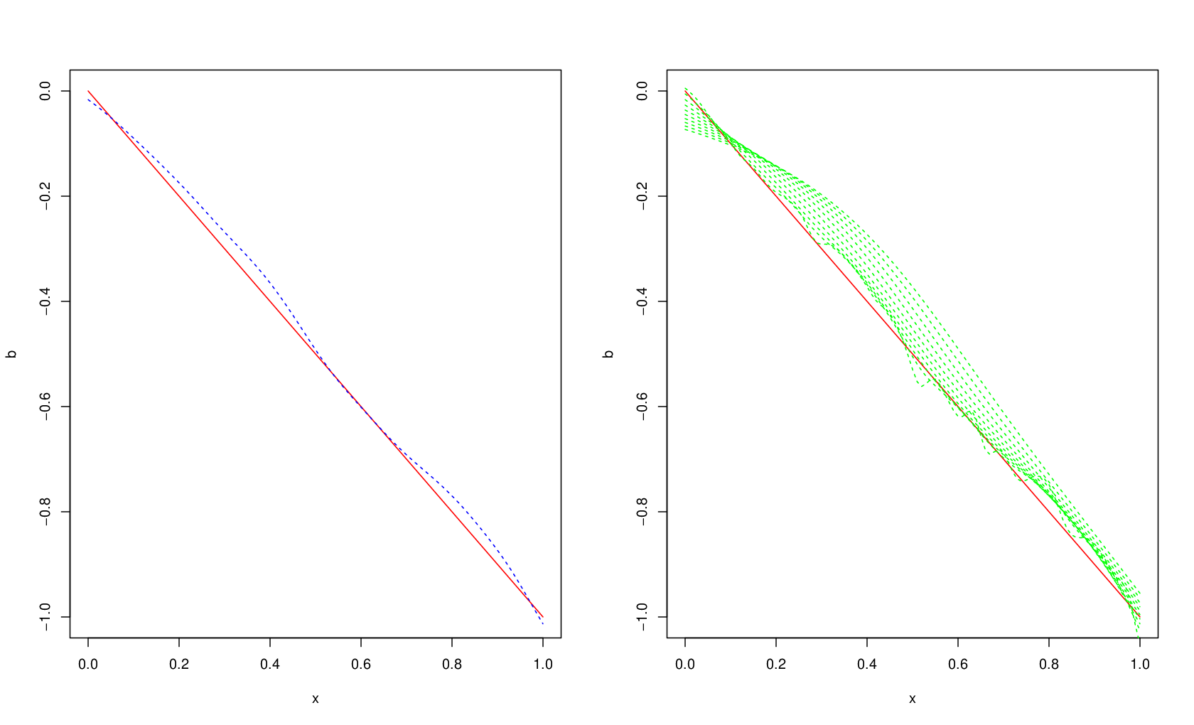
Some numerical experiments on our estimation method are presented in this subsection. The discrete-time approximate Nadaraya-Watson (NW) (see (5)) estimator is computed on 4 datasets generated by SDEs with various types of vector fields. In each case, the bandwidth of the NW estimator is selected via the looCV method introduced at Subsection 5.2. On the one hand, two models with the same linear drift function are considered, but with an additive noise for the first one and a multiplicative noise for the second one:

  • 1.

    The so-called Langevin equation, that is

    Xt=x0−∫0tXs​𝑑s+0.1⋅Wt.X_{t}=x_{0}-\int_{0}^{t}X_{s}ds+0.1\cdot W_{t}.
  • 2.

    The hyperbolic diffusion process, that is

    Xt=x0−∫0tXs​𝑑s+0.1​∫0t1+Xs2​d​Ws.X_{t}=x_{0}-\int_{0}^{t}X_{s}ds+0.1\int_{0}^{t}\sqrt{1+X_{s}^{2}}dW_{s}.

On the other hand, two models having the same non-linear drift function involving sin(.)\sin(.) are considered, but here again with an additive noise for the first one and a multiplicative noise for the second one:

  • 3.

    The third model is defined by

    Xt=x0−∫0t(Xs+sin⁡(4​Xs))​𝑑s+0.1⋅Wt.X_{t}=x_{0}-\int_{0}^{t}(X_{s}+\sin(4X_{s}))ds+0.1\cdot W_{t}.
  • 4.

    The fourth model is defined by

    Xt=x0−∫0t(Xs+sin⁡(4​Xs))​𝑑s+0.1​∫0t(2+cos⁡(Xs))​d​Ws.X_{t}=x_{0}-\int_{0}^{t}(X_{s}+\sin(4X_{s}))ds+0.1\int_{0}^{t}(2+\cos(X_{s}))dW_{s}.

The models and the estimator are implemented by taking N=200N=200, n=50n=50, T=5T=5, x0=2x_{0}=2, t0=1t_{0}=1 and KK the Gaussian kernel z↦(2π)−1/2e−z2/2z\mapsto(2\pi)^{-1/2}e^{-z^{2}/2}. For Models 1 and 2, the estimator of the drift function is computed for the bandwidths set

ℋ1:={0.02​k​ ; ​k=1,…,10},\mathcal{H}_{1}:=\{0.02k\textrm{ $;$ }k=1,\dots,10\},

and for Models 3 and 4, it is computed for the bandwidths set

ℋ2:={0.01​k​ ; ​k=1,…,10}.\mathcal{H}_{2}:=\{0.01k\textrm{ $;$ }k=1,\dots,10\}.

Each set of bandwidths has been chosen after testing different values of hh, to see with which ones the estimation performs better. To choose smaller values in the second set of bandwidths allows to check that the looCV method does not systematically select the smallest bandwidth for Models 3 and 4.

For each of the previous models, on Figures 1, 2, 3 and 4 respectively, the true drift function (in red) and the looCV adaptive NW estimator (in blue) are plotted on the left-hand side, and the beam of proposals is plotted in green on the right-hand side. On Figures 1 and 2, one can see that the drift function is well estimated by the looCV adaptive NW estimator, with a MSE equal to 2.95⋅10−42.95\cdot 10^{-4} for the Langevin equation and to 8.31⋅10−48.31\cdot 10^{-4} for the hyperbolic diffusion process. As presumed, the multiplicative noise in Model 2 slightly degrades the MSE. Note that when the bandwidth is too small, the estimation degrades, but the looCV method selects a higher value of hh which performs better on the estimation. This means that, as expected, the looCV method selects a reasonable approximation of the bandwidth for which the NW estimator reaches the bias-variance tradeoff. On Figures 3 and 4, one can see that the drift function of Models 3 and 4 is still well estimated by our looCV adaptive NW estimator. However, note that there is a significant degradation of the MSE, which is equal to 2.89⋅10−32.89\cdot 10^{-3} for Model 3 and to 9.26⋅10−39.26\cdot 10^{-3} for Model 4. This is probably related to the nonlinearity of the drift function to estimate. Once again, to consider a multiplicative noise in Model 4 degrades the estimation quality with respect to Model 3. As for Models 1 and 2, note that the looCV does not systematically select the smallest bandwidth.

Refer to caption
Figure 1. LooCV NW estimation for Model 1 (Langevin equation), h^=0.04\widehat{h}=0.04.
Refer to caption
Figure 2. LooCV NW estimation for Model 2 (hyperbolic diffusion process), h^=0.04\widehat{h}=0.04.
Refer to caption
Figure 3. LooCV NW estimation for Model 3, h^=0.02\widehat{h}=0.02.
Refer to caption
Figure 4. LooCV NW estimation for Model 4, h^=0.06\widehat{h}=0.06.


For Model 1, at levels n=10,20,…,100n=10,20,\dots,100, Figure 5 shows the evolution of the MSE of the looCV adaptive NW estimator as a function of NN. For this study, the value of NN ranges from 2020 to 200200. Figure 5 shows that the MSE of our adaptive estimator remains low regardless to the value of (n,N)(n,N) (from 4.50⋅10−54.50\cdot 10^{-5} to 9.01⋅10−39.01\cdot 10^{-3}), decreases when NN increases (for each nn), and decreases when nn increases (for a fixed NN). This is consistent with the risk bounds of Section 4. Note also that for N⩾70N\geqslant 70, there is no significant gain to take nn larger than 3030. For Model 3, Figure 6 shows the evolution of the MSE of the looCV adaptive NW estimator as a function of NN and leads to the same conclusions than for Model 1. Note anyway that due to the nonlinearity of bb, the MSE of our adaptive estimator reaches higher values (from 2.67⋅10−42.67\cdot 10^{-4} to 4.49⋅10−24.49\cdot 10^{-2}) than for Model 1. Again, there is no significant gain to take nn larger than 3030, and above all larger than 7070.

Refer to caption
Figure 5. MSE of the looCV estimator with respect to NN and nn for Model 1.
Refer to caption
Figure 6. MSE of the looCV estimator with respect to NN and nn for Model 3.


Finally, for each model, Table 1 gathers the mean MSE of 100 looCV NW estimations of the drift function as well as the mean MSE of the corresponding 100 oracle estimations. The mean MSEs are globally low, but significantly higher for the models with a nonlinear drift function (Models 3 and 4) than for the models with a linear one (Models 1 and 2). Moreover, for each drift function, the mean MSE is slightly degraded for the models with a multiplicative noise (Models 2 and 4) with respect to the models with an additive one (Models 1 and 3). Note also that for each model, the mean MSE of the looCV estimations is close to the mean MSE of the corresponding oracle estimations. This means that our looCV method performs well in practice.

looCV Oracle
Model 1 3.03⋅10−43.03\cdot 10^{-4} 2.67⋅10−42.67\cdot 10^{-4}
Model 2 6.52⋅10−46.52\cdot 10^{-4} 4.96⋅10−44.96\cdot 10^{-4}
Model 3 2.45⋅10−32.45\cdot 10^{-3} 1.99⋅10−31.99\cdot 10^{-3}
Model 4 9.15⋅10−39.15\cdot 10^{-3} 6.02⋅10−36.02\cdot 10^{-3}
Table 1. Mean MSEs of 100 looCV adaptive NW estimations compared to the oracle estimations.
Remark 5.6.

Note that to take t0⩾1t_{0}\geqslant 1 (here t0=1t_{0}=1) is recommended even in numerical experiments. Indeed, for instance, the mean MSE of 10 looCV estimations for Model 1 is significantly lower with t0=1t_{0}=1 (2.49⋅10−42.49\cdot 10^{-4}) than with t0=0t_{0}=0 (3.82⋅10−33.82\cdot 10^{-3}).

6. Concluding remarks

In this paper, first, a risk bound on our continuous-time Nadaraya-Watson estimator of bb has been established. This bound is satisfactory because it leads to a rate of same order than in the classic nonparametric regression framework (see Comte [2], Chapter 4), and of same order than in Della Maestra and Hoffmann [13] for their estimator of the drift function in McKean-Vlasov models. Then, a risk bound on a discrete-time approximate estimator of bb has been established too. The bound is satisfactory when bb and σ\sigma are bounded, but a bit degraded when bb is unbounded. To improve this bound will be the subject of future investigations.

In a second part, two bandwidth selection methods are provided. The first one is an extension of the PCO method to the 2bNW estimator of bb in the spirit of Comte and Marie [8]. An oracle inequality is established but under the condition (N​h3)−1⩽1(Nh^{3})^{-1}\leqslant 1 (instead of (N​h)−1⩽1(Nh)^{-1}\leqslant 1) on the bandwidths collection. Unfortunately, it seems difficult to bypass this condition because of some constants involved in Bernstein’s inequality and in the concentration inequality for U-statistics of Giné and Nickl [17] (see Subsection A.7), but as explained at Remark 5.4 this condition is not so bad. The second bandwidth selection method is an extension of the looCV procedure for the discrete-time approximate estimator written has a convex combination. As in the nonparametric regression framework, this method is numerically satisfactory but it seems difficult to establish a theoretical risk bound on the associated adaptive estimator.

Finally, the estimation of bb has been only investigated in the case of one-dimensional diffusion processes because of its simplicity, but by following the same ideas than Halconruy and Marie used in the nonparametric regression framework in [19], the major part of the results of the present paper should be extendable to multidimensional diffusion processes.

References

  • [1] A. Cohen, M.A. Leviatan and D. Leviatan. On the Stability and Accuracy of Least Squares Approximations. Found. Comput. Math. 13, 819-834, 2013.
  • [2] F. Comte. Estimation non-paramétrique. 2e édition. Spartacus IDH, 2017.
  • [3] F. Comte and V. Genon-Catalot. Regression Function Estimation on Non Compact Support as a Partly Inverse Problem. The Annals of the Institute of Statistical Mathematics 72, 4, 1023-1054, 2020.
  • [4] F. Comte and V. Genon-Catalot. Nonparametric Drift Estimation for i.i.d. Paths of Stochastic Differential Equations. The Annals of Statistics 48, 6, 3336-3365, 2020.
  • [5] F. Comte and V. Genon-Catalot. Drift Estimation on Non Compact Support for Diffusion Models. Stoch. Proc. Appl. 134, 174-207, 2021.
  • [6] F. Comte, V. Genon-Catalot and Y. Rozenholc. Penalized Nonparametric Mean Square Estimation of the Coefficients of Diffusion Processes. Bernoulli 12, 2, 514-543, 2007.
  • [7] F. Comte, V. Genon-Catalot and A. Samson. Nonparametric Estimation for Stochastic Differential Equations with Random Effects. Stoch. Proc. Appl. 123, 2522-2551, 2013.
  • [8] F. Comte and N. Marie. On a Nadaraya-Watson Estimator with Two Bandwidths. Electronic Journal of Statistics 15, 1, 2566-2607, 2021.
  • [9] A. Dalalyan. Sharp Adaptive Estimation of the Trend Coefficient for Ergodic Diffusion. The Annals of Statistics 33, 6, 2507-2528, 2005.
  • [10] M. Delattre, V. Genon-Catalot and C. Larédo. Parametric Inference for Discrete Observations of Diffusion Processes with Mixed Effects. Stoch. Proc. Appl. 128, 1929-1957, 2018.
  • [11] M. Delattre, V. Genon-Catalot and A. Samson. Maximum Likelihood Estimation for Stochastic Differential Equations with Random Effects. Scand. J. Stat. 40, 322-343, 2013.
  • [12] M. Delattre and M. Lavielle. Coupling the SAEM Algorithm and the Extended Kalman Filter for Maximum Likelihood Estimation in Mixed-Effects Diffusion Models. Stat. Interface 6, 519-532, 2013.
  • [13] L. Della Maestra and M. Hoffmann. Nonparametric Estimation for Interacting Particle Systems: McKean-Vlasov Models. To appear in Probability Theory and Related Fields, 2021.
  • [14] C. Denis, C. Dion and M. Martinez. A Ridge Estimator of the Drift from Discrete Repeated Observations of the Solutions of a Stochastic Differential Equation. To appear in Bernoulli, 2021.
  • [15] C. Dion and V. Genon-Catalot. Bidimensional Random Effect Estimation in Mixed Stochastic Differential Model. Stat. Inference Stoch. Process. 19, 131-158, 2016.
  • [16] S. Ditlevsen and A. De Gaetano. Mixed Effects in Stochastic Differential Equation Models. REVSTAT 3, 137-153, 2005.
  • [17] E. Giné and R. Nickl. Mathematical Foundations of Infinite-Dimensional Statistical Models. Cambridge University Press, 2015.
  • [18] L. Györfi, M. Kohler, A. Krzyzak and H. Walk. A Distribution-Free Theory of Nonparametric Regression. Springer Series in Statistics. Springer-Verlag, New York, 2002.
  • [19] H. Halconruy and N. Marie. Kernel Selection in Nonparametric Regression. Mathematical Methods of Statistics 29, 1, 32-56, 2020.
  • [20] M. Hoffmann. Adaptive Estimation in Diffusion Processes. Stoch. Proc. Appl. 79, 135-163, 1999.
  • [21] C. Houdré and P. Reynaud-Bouret. Exponential Inequalities, with Constants, for U-statistics of Order Two. Stochastic Inequalities and Applications, vol. 56 of Progr. Proba, 55-69, Birkhauser, 2003.
  • [22] M. Kessler. Simple and Explicit Estimating Functions for a Discretely Observed Diffusion Process. Scandinavian Journal of Statistics 27, 1, 65-82, 2000.
  • [23] S. Kusuoka and D. Stroock. Applications of the Malliavin Calculus, Part II. J. Fac. Sci. Univ. Tokyo 32, 1-76, 1985.
  • [24] Y. Kutoyants. Statistical Inference for Ergodic Diffusion Processes. Springer, 2004.
  • [25] C. Lacour, P. Massart and V. Rivoirard. Estimator Selection: New Method with Applications to Kernel Density Estimation. Sankhia A 79, 2, 298-335, 2017.
  • [26] S. Menozzi, A. Pesce and X. Zhang. Density and Gradient Estimates for Non Degenerate Brownian SDEs with Unbounded Measurable Drift. Journal of Differential Equations 272, 330-369, 2021.
  • [27] R. Overgaard, N. Jonsson, C. Tornoe, H. Madsen. Non-Linear Mixed Effects Models with Stochastic Differential Equations: Implementation of an Estimation Algorithm. J. Pharmacokinet. Pharmacodyn. 32, 85-107, 2005.
  • [28] U. Picchini, A. De Gaetano and S. Ditlevsen. Stochastic Differential Mixed-Effects Models. Scand. J. Stat. 37, 67-90, 2010.
  • [29] U. Picchini and S. Ditlevsen. Practical Estimation of High Dimensional Stochastic Differential Mixed-Effects Models. Comput. Statist. Data Anal. 55, 1426-1444, 2011.

Appendix A Proofs

A.1. Proof of Corollary 2.5

First of all, since pt​(x0,x)>0p_{t}(x_{0},x)>0 for every (t,x)∈(0,T]×ℝ(t,x)\in(0,T]\times\mathbb{R},

f⁡(x)=1T−t0​∫t0Tpt​(x0,x)​𝑑t>0f(x)=\frac{1}{T-t_{0}}\int_{t_{0}}^{T}p_{t}(x_{0},x)dt>0

for every x∈ℝx\in\mathbb{R}. Consider ℓ∈{0,…,β−1}\ell\in\{0,\dots,\beta-1\} and θ∈ℝ+\theta\in\mathbb{R}_{+}. Thanks to the bound on (t,x)↦∂xℓ+1pt​(x0,x)(t,x)\mapsto\partial_{x}^{\ell+1}p_{t}(x_{0},x) given in Assumption 2.2,

∥f(ℓ)(⋅+θ)−f(ℓ)∥22=∫−∞∞[f(ℓ)(x+x0+θ)−f(ℓ)(x+x0)]2dx\displaystyle\|f^{(\ell)}(\cdot+\theta)-f^{(\ell)}\|_{2}^{2}=\int_{-\infty}^{\infty}[f^{(\ell)}(x+x_{0}+\theta)-f^{(\ell)}(x+x_{0})]^{2}dx
⩽1T−t0​∫t0T∫−∞∞(∂2ℓpt​(x0,x+x0+θ)−∂2ℓpt​(x0,x+x0))2​𝑑x​𝑑t\displaystyle\hskip 28.45274pt\leqslant\frac{1}{T-t_{0}}\int_{t_{0}}^{T}\int_{-\infty}^{\infty}(\partial_{2}^{\ell}p_{t}(x_{0},x+x_{0}+\theta)-\partial_{2}^{\ell}p_{t}(x_{0},x+x_{0}))^{2}dxdt
⩽θ2T−t0​∫t0T∫−∞∞supz∈[x,x+θ]|∂2ℓ+1pt​(x0,z+x0)|2​𝑑x​𝑑t\displaystyle\hskip 28.45274pt\leqslant\frac{\theta^{2}}{T-t_{0}}\int_{t_{0}}^{T}\int_{-\infty}^{\infty}\sup_{z\in[x,x+\theta]}|\partial_{2}^{\ell+1}p_{t}(x_{0},z+x_{0})|^{2}dxdt
⩽𝔠2.2,2​(ℓ+1)2​θ2T−t0​∫t0T1t2​q2​(ℓ+1)​∫−∞∞supz∈[x,x+θ]exp⁡(−2​𝔪2.2,2​(ℓ+1)​z2t)​𝑑x​𝑑t\displaystyle\hskip 28.45274pt\leqslant\mathfrak{c}_{\ref{assumption_bound_derivative_density_x},2}(\ell+1)^{2}\frac{\theta^{2}}{T-t_{0}}\int_{t_{0}}^{T}\frac{1}{t^{2q_{2}(\ell+1)}}\int_{-\infty}^{\infty}\sup_{z\in[x,x+\theta]}\exp\left(-2\mathfrak{m}_{\ref{assumption_bound_derivative_density_x},2}(\ell+1)\frac{z^{2}}{t}\right)dxdt
=𝔠2.2,2(ℓ+1)2θ2T−t0∫t0T1t2​q2​(ℓ+1)×\displaystyle\hskip 28.45274pt=\mathfrak{c}_{\ref{assumption_bound_derivative_density_x},2}(\ell+1)^{2}\frac{\theta^{2}}{T-t_{0}}\int_{t_{0}}^{T}\frac{1}{t^{2q_{2}(\ell+1)}}\times
[∫−∞−θexp⁡(−2​𝔪2.2,2​(ℓ+1)​(x+θ)2t)​𝑑x+θ+∫0∞exp⁡(−2​𝔪2.2,2​(ℓ+1)​x2t)​𝑑x]​𝑑t\displaystyle\hskip 56.9055pt\left[\int_{-\infty}^{-\theta}\exp\left(-2\mathfrak{m}_{\ref{assumption_bound_derivative_density_x},2}(\ell+1)\frac{(x+\theta)^{2}}{t}\right)dx+\theta+\int_{0}^{\infty}\exp\left(-2\mathfrak{m}_{\ref{assumption_bound_derivative_density_x},2}(\ell+1)\frac{x^{2}}{t}\right)dx\right]dt
⩽1t02​q2​(ℓ+1)​[𝔠1​θ2+θ3​maxk∈{0,…,β−1}​𝔠2.2,2​(k+1)2]\displaystyle\hskip 28.45274pt\leqslant\frac{1}{t_{0}^{2q_{2}(\ell+1)}}\left[\mathfrak{c}_{1}\theta^{2}+\theta^{3}\max_{k\in\{0,\dots,\beta-1\}}\mathfrak{c}_{\ref{assumption_bound_derivative_density_x},2}(k+1)^{2}\right]

with

𝔠1=2​maxk∈{0,…,β−1}​{𝔠2.2,2​(k+1)2​∫0∞exp⁡(−2​𝔪2.2,2​(k+1)​x2T)​𝑑x},\mathfrak{c}_{1}=2\max_{k\in\{0,\dots,\beta-1\}}\left\{\mathfrak{c}_{\ref{assumption_bound_derivative_density_x},2}(k+1)^{2}\int_{0}^{\infty}\exp\left(-2\mathfrak{m}_{\ref{assumption_bound_derivative_density_x},2}(k+1)\frac{x^{2}}{T}\right)dx\right\},

and the same way,

∥f(ℓ)(⋅−θ)−f(ℓ)∥22⩽θ2T−t0∫t0T∫−∞∞supz∈[x−θ,x]|∂2ℓ+1pt(x0,z+x0)|2dxdt\displaystyle\|f^{(\ell)}(\cdot-\theta)-f^{(\ell)}\|_{2}^{2}\leqslant\frac{\theta^{2}}{T-t_{0}}\int_{t_{0}}^{T}\int_{-\infty}^{\infty}\sup_{z\in[x-\theta,x]}|\partial_{2}^{\ell+1}p_{t}(x_{0},z+x_{0})|^{2}dxdt
⩽𝔠2.2,2(ℓ+1)2θ2T−t0∫t0T1t2​q2​(ℓ+1)×\displaystyle\hskip 28.45274pt\leqslant\mathfrak{c}_{\ref{assumption_bound_derivative_density_x},2}(\ell+1)^{2}\frac{\theta^{2}}{T-t_{0}}\int_{t_{0}}^{T}\frac{1}{t^{2q_{2}(\ell+1)}}\times
[∫−∞0exp⁡(−2​𝔪2.2,2​(ℓ+1)​x2t)​𝑑x+θ+∫θ∞exp⁡(−2​𝔪2.2,2​(ℓ+1)​(x−θ)2t)​𝑑x]​𝑑t\displaystyle\hskip 56.9055pt\left[\int_{-\infty}^{0}\exp\left(-2\mathfrak{m}_{\ref{assumption_bound_derivative_density_x},2}(\ell+1)\frac{x^{2}}{t}\right)dx+\theta+\int_{\theta}^{\infty}\exp\left(-2\mathfrak{m}_{\ref{assumption_bound_derivative_density_x},2}(\ell+1)\frac{(x-\theta)^{2}}{t}\right)dx\right]dt
⩽1t02​q2​(ℓ+1)​[𝔠1​θ2+θ3​maxk∈{0,…,β−1}​𝔠2.2,2​(k+1)2].\displaystyle\hskip 28.45274pt\leqslant\frac{1}{t_{0}^{2q_{2}(\ell+1)}}\left[\mathfrak{c}_{1}\theta^{2}+\theta^{3}\max_{k\in\{0,\dots,\beta-1\}}\mathfrak{c}_{\ref{assumption_bound_derivative_density_x},2}(k+1)^{2}\right].

This concludes the proof.

A.2. Proof of Proposition 3.3

First of all, the bias of f^N,h​(x)\widehat{f}_{N,h}(x) is denoted by 𝔟⁡(x)\mathfrak{b}(x) and its variance by 𝔳⁡(x)\mathfrak{v}(x). Moreover, let us recall the bias-variance decomposition of the 𝕃2\mathbb{L}^{2}-risk of f^N,h\widehat{f}_{N,h}:

𝔼⁡(‖f^N,h−f‖22)=∫−∞∞𝔟​(x)2​𝑑x+∫−∞∞𝔳⁡(x)​𝑑x.\displaystyle\mathbb{E}(\|\widehat{f}_{N,h}-f\|_{2}^{2})=\int_{-\infty}^{\infty}\mathfrak{b}(x)^{2}dx+\int_{-\infty}^{\infty}\mathfrak{v}(x)dx.

On the one hand, let us find a suitable bound on the integrated variance of f^N,h\widehat{f}_{N,h}. Since X1,…,XNX^{1},\dots,X^{N} are i.i.d. copies of XX, and thanks to Jensen’s inequality,

𝔳⁡(x)\displaystyle\mathfrak{v}(x) =\displaystyle= var⁡(1N⁡(T−t0)​∑i=1N∫t0TKh​(Xti−x)​𝑑t)\displaystyle\mathrm{var}\left(\frac{1}{N(T-t_{0})}\sum_{i=1}^{N}\int_{t_{0}}^{T}K_{h}(X_{t}^{i}-x)dt\right)
=\displaystyle= 1N​(T−t0)2​var​(∫t0TKh​(Xt−x)​𝑑t)⩽1N​𝔼​[(∫t0TKh​(Xt−x)​d​tT−t0)2]\displaystyle\frac{1}{N(T-t_{0})^{2}}\mathrm{var}\left(\int_{t_{0}}^{T}K_{h}(X_{t}-x)dt\right)\leqslant\frac{1}{N}\mathbb{E}\left[\left(\int_{t_{0}}^{T}K_{h}(X_{t}-x)\frac{dt}{T-t_{0}}\right)^{2}\right]
⩽\displaystyle\leqslant 1N⁡(T−t0)​∫t0T𝔼⁡(Kh​(Xt−x)2)​𝑑t=1N​∫−∞∞Kh​(z−x)2​f​(z)​𝑑z.\displaystyle\frac{1}{N(T-t_{0})}\int_{t_{0}}^{T}\mathbb{E}(K_{h}(X_{t}-x)^{2})dt=\frac{1}{N}\int_{-\infty}^{\infty}K_{h}(z-x)^{2}f(z)dz.

Thus, since KK is symmetric,

∫−∞∞𝔳⁡(x)​𝑑x\displaystyle\int_{-\infty}^{\infty}\mathfrak{v}(x)dx ⩽\displaystyle\leqslant 1N​∫−∞∞f⁡(z)​∫−∞∞Kh​(z−x)2​𝑑x​𝑑z\displaystyle\frac{1}{N}\int_{-\infty}^{\infty}f(z)\int_{-\infty}^{\infty}K_{h}(z-x)^{2}dxdz
=\displaystyle= 1N​h​(∫−∞∞f⁡(z)​𝑑z)​(∫−∞∞K​(x)2​𝑑x)=‖K‖22N​h.\displaystyle\frac{1}{Nh}\left(\int_{-\infty}^{\infty}f(z)dz\right)\left(\int_{-\infty}^{\infty}K(x)^{2}dx\right)=\frac{\|K\|_{2}^{2}}{Nh}.

On the other hand, let us find a suitable bound on the integrated squared-bias of f^N,h​(x)\widehat{f}_{N,h}(x). Since X1,…,XNX^{1},\dots,X^{N} are i.i.d. copies of XX,

𝔟⁡(x)\displaystyle\mathfrak{b}(x) =\displaystyle= 1T−t0​∫t0T𝔼⁡(Kh​(Xt−x))​𝑑t−f⁡(x)\displaystyle\frac{1}{T-t_{0}}\int_{t_{0}}^{T}\mathbb{E}(K_{h}(X_{t}-x))dt-f(x)
=\displaystyle= 1h​∫−∞∞K⁡(z−xh)​f​(z)​𝑑z−f⁡(x)\displaystyle\frac{1}{h}\int_{-\infty}^{\infty}K\left(\frac{z-x}{h}\right)f(z)dz-f(x)
=\displaystyle= ∫−∞∞K⁡(z)​(f⁡(h​z+x)−f⁡(x))​𝑑z.\displaystyle\int_{-\infty}^{\infty}K(z)(f(hz+x)-f(x))dz.

First, assume that β=1\beta=1. By Assumption 3.2, the generalized Minkowski inequality and Corollary 2.5,

∫−∞∞𝔟​(x)2​𝑑x\displaystyle\int_{-\infty}^{\infty}\mathfrak{b}(x)^{2}dx ⩽\displaystyle\leqslant ∫−∞∞(∫−∞∞K⁡(z)​(f⁡(h​z+x)−f⁡(x))​𝑑z)2​𝑑x\displaystyle\int_{-\infty}^{\infty}\left(\int_{-\infty}^{\infty}K(z)(f(hz+x)-f(x))dz\right)^{2}dx
⩽\displaystyle\leqslant [∫−∞∞K⁡(z)​(∫−∞∞(f⁡(h​z+x)−f⁡(x))2​𝑑x)1/2​𝑑z]2⩽𝔠1​(t0)​h2\displaystyle\left[\int_{-\infty}^{\infty}K(z)\left(\int_{-\infty}^{\infty}(f(hz+x)-f(x))^{2}dx\right)^{1/2}dz\right]^{2}\leqslant\mathfrak{c}_{1}(t_{0})h^{2}

with

𝔠1​(t0)=𝔠2.5t02​q2​(1)​(∫−∞∞|z|​(1+|z|1/2)​|K⁡(z)|​𝑑z)2.\mathfrak{c}_{1}(t_{0})=\frac{\mathfrak{c}_{\ref{Nikolskii_f}}}{t_{0}^{2q_{2}(1)}}\left(\int_{-\infty}^{\infty}|z|(1+|z|^{1/2})|K(z)|dz\right)^{2}.

Now, assume that β⩾2\beta\geqslant 2. By the Taylor formula with integral remainder, for every z∈ℝz\in\mathbb{R},

f⁡(h​z+x)−f⁡(x)=𝟏β⩾3​∑ℓ=1β−2(h​z)ℓℓ!​f(ℓ)​(x)+(h​z)β−1(β−2)!​∫01(1−τ)β−2​f(β−1)​(τ​h​z+x)​𝑑τ.f(hz+x)-f(x)=\mathbf{1}_{\beta\geqslant 3}\sum_{\ell=1}^{\beta-2}\frac{(hz)^{\ell}}{\ell!}f^{(\ell)}(x)+\frac{(hz)^{\beta-1}}{(\beta-2)!}\int_{0}^{1}(1-\tau)^{\beta-2}f^{(\beta-1)}(\tau hz+x)d\tau.

Then, by Assumption 3.2, the generalized Minkowski inequality (two times) and Corollary 2.5,

∫−∞∞𝔟​(x)2​𝑑x=∫−∞∞(∫−∞∞K⁡(z)​(f⁡(h​z+x)−f⁡(x))​𝑑z)2​𝑑x\displaystyle\int_{-\infty}^{\infty}\mathfrak{b}(x)^{2}dx=\int_{-\infty}^{\infty}\left(\int_{-\infty}^{\infty}K(z)(f(hz+x)-f(x))dz\right)^{2}dx
=h2​(β−1)|(β−2)!|2​∫−∞∞(∫−∞∞zβ−1​K​(z)​∫01(1−τ)β−2​[f(β−1)​(τ​h​z+x)−f(β−1)​(x)]​𝑑τ​𝑑z)2​𝑑x\displaystyle\hskip 28.45274pt=\frac{h^{2(\beta-1)}}{|(\beta-2)!|^{2}}\int_{-\infty}^{\infty}\left(\int_{-\infty}^{\infty}z^{\beta-1}K(z)\int_{0}^{1}(1-\tau)^{\beta-2}[f^{(\beta-1)}(\tau hz+x)-f^{(\beta-1)}(x)]d\tau dz\right)^{2}dx
⩽h2​(β−1)|(β−2)!|2×\displaystyle\hskip 28.45274pt\leqslant\frac{h^{2(\beta-1)}}{|(\beta-2)!|^{2}}\times
[∫−∞∞|z|β−1​|K⁡(z)|​∫01(1−τ)β−2​(∫−∞∞[f(β−1)​(τ​h​z+x)−f(β−1)​(x)]2​𝑑x)1/2​𝑑τ​𝑑z]2\displaystyle\hskip 56.9055pt\left[\int_{-\infty}^{\infty}|z|^{\beta-1}|K(z)|\int_{0}^{1}(1-\tau)^{\beta-2}\left(\int_{-\infty}^{\infty}[f^{(\beta-1)}(\tau hz+x)-f^{(\beta-1)}(x)]^{2}dx\right)^{1/2}d\tau dz\right]^{2}
⩽𝔠2.5​h2​β|(β−2)!|2​t02​q2​(β)​(∫−∞∞|z|β−1​|K⁡(z)|​∫01(1−τ)β−2​[τ​|z|+(τ​|z|)3/2]​𝑑τ​𝑑z)2⩽𝔠2​(t0)​h2​β\displaystyle\hskip 28.45274pt\leqslant\frac{\mathfrak{c}_{\ref{Nikolskii_f}}h^{2\beta}}{|(\beta-2)!|^{2}t_{0}^{2q_{2}(\beta)}}\left(\int_{-\infty}^{\infty}|z|^{\beta-1}|K(z)|\int_{0}^{1}(1-\tau)^{\beta-2}[\tau|z|+(\tau|z|)^{3/2}]d\tau dz\right)^{2}\leqslant\mathfrak{c}_{2}(t_{0})h^{2\beta}

with

𝔠2​(t0)=𝔠2.5|(β−2)!|2​t02​q2​(β)​(∫−∞∞|z|β​(1+|z|1/2)​|K⁡(z)|​𝑑z)2.\mathfrak{c}_{2}(t_{0})=\frac{\mathfrak{c}_{\ref{Nikolskii_f}}}{|(\beta-2)!|^{2}t_{0}^{2q_{2}(\beta)}}\left(\int_{-\infty}^{\infty}|z|^{\beta}(1+|z|^{1/2})|K(z)|dz\right)^{2}.

This concludes the proof.

A.3. Proof of Proposition 3.4

First of all,

𝔼⁡(‖b​f^N,h−b​f‖22)=∫−∞∞𝔟​(x)2​𝑑x+∫−∞∞𝔳⁡(x)​𝑑x\displaystyle\mathbb{E}(\|\widehat{bf}_{N,h}-bf\|_{2}^{2})=\int_{-\infty}^{\infty}\mathfrak{b}(x)^{2}dx+\int_{-\infty}^{\infty}\mathfrak{v}(x)dx

where 𝔟⁡(x)\mathfrak{b}(x) (resp. 𝔳⁡(x)\mathfrak{v}(x)) is the bias (resp. the variance) term of b​f^N,h​(x)\widehat{bf}_{N,h}(x) for any x∈ℝx\in\mathbb{R}. On the one hand, let us find a suitable bound on the integrated variance of b​f^N,h\widehat{bf}_{N,h}. Since X1,…,XNX^{1},\dots,X^{N} are i.i.d. copies of XX,

𝔳⁡(x)\displaystyle\mathfrak{v}(x) =\displaystyle= var​(1N⁡(T−t0)​∑i=1N∫t0TKh​(Xti−x)​d​Xti)⩽1N​(T−t0)2​𝔼​[(∫t0TKh​(Xt−x)​d​Xt)2]\displaystyle\textrm{var}\left(\frac{1}{N(T-t_{0})}\sum_{i=1}^{N}\int_{t_{0}}^{T}K_{h}(X_{t}^{i}-x)dX_{t}^{i}\right)\leqslant\frac{1}{N(T-t_{0})^{2}}\mathbb{E}\left[\left(\int_{t_{0}}^{T}K_{h}(X_{t}-x)dX_{t}\right)^{2}\right]
⩽\displaystyle\leqslant 2N​𝔼​[(∫t0TKh​(Xt−x)​b​(Xt)​d​tT−t0)2+1(T−t0)2​(∫t0TKh​(Xt−x)​σ​(Xt)​d​Wt)2].\displaystyle\frac{2}{N}\mathbb{E}\left[\left(\int_{t_{0}}^{T}K_{h}(X_{t}-x)b(X_{t})\frac{dt}{T-t_{0}}\right)^{2}+\frac{1}{(T-t_{0})^{2}}\left(\int_{t_{0}}^{T}K_{h}(X_{t}-x)\sigma(X_{t})dW_{t}\right)^{2}\right].

In the right-hand side of the previous inequality, Jensen’s inequality on the first term and the isometry property for Itô’s integral on the second one give

𝔳⁡(x)\displaystyle\mathfrak{v}(x) ⩽\displaystyle\leqslant 2N⁡(T−t0)​∫t0T𝔼⁡[Kh​(Xt−x)2​b​(Xt)2]​𝑑t+2N​(T−t0)2​∫t0T𝔼⁡[Kh​(Xt−x)2​σ​(Xt)2]​𝑑t\displaystyle\frac{2}{N(T-t_{0})}\int_{t_{0}}^{T}\mathbb{E}[K_{h}(X_{t}-x)^{2}b(X_{t})^{2}]dt+\frac{2}{N(T-t_{0})^{2}}\int_{t_{0}}^{T}\mathbb{E}[K_{h}(X_{t}-x)^{2}\sigma(X_{t})^{2}]dt
=\displaystyle= 2N​∫−∞∞Kh​(z−x)2​b​(z)2​f​(z)​𝑑z+2N⁡(T−t0)​∫−∞∞Kh​(z−x)2​σ​(z)2​f​(z)​𝑑z.\displaystyle\frac{2}{N}\int_{-\infty}^{\infty}K_{h}(z-x)^{2}b(z)^{2}f(z)dz+\frac{2}{N(T-t_{0})}\int_{-\infty}^{\infty}K_{h}(z-x)^{2}\sigma(z)^{2}f(z)dz.

Moreover, KK is symmetric and K∈𝕃2​(ℝ,d​x)K\in\mathbb{L}^{2}(\mathbb{R},dx) by Assumption 3.1, and b,σ∈𝕃2​(ℝ,f⁡(x)​d​x)b,\sigma\in\mathbb{L}^{2}(\mathbb{R},f(x)dx) by Remark 2.4. Then,

∫−∞∞𝔳⁡(x)​𝑑x\displaystyle\int_{-\infty}^{\infty}\mathfrak{v}(x)dx ⩽\displaystyle\leqslant 2N​∫ℝ2Kh​(z−x)2​b​(z)2​f​(z)​𝑑z​𝑑x+2N⁡(T−t0)​∫ℝ2Kh​(z−x)2​σ​(z)2​f​(z)​𝑑z​𝑑x\displaystyle\frac{2}{N}\int_{\mathbb{R}^{2}}K_{h}(z-x)^{2}b(z)^{2}f(z)dzdx+\frac{2}{N(T-t_{0})}\int_{\mathbb{R}^{2}}K_{h}(z-x)^{2}\sigma(z)^{2}f(z)dzdx
=\displaystyle= 2N​h​∫−∞∞b​(z)2​f​(z)​∫−∞∞K​(x)2​𝑑x​𝑑z+2N⁡(T−t0)​h​∫−∞∞σ​(z)2​f​(z)​∫−∞∞K​(x)2​𝑑x​𝑑z\displaystyle\frac{2}{Nh}\int_{-\infty}^{\infty}b(z)^{2}f(z)\int_{-\infty}^{\infty}K(x)^{2}dxdz+\frac{2}{N(T-t_{0})h}\int_{-\infty}^{\infty}\sigma(z)^{2}f(z)\int_{-\infty}^{\infty}K(x)^{2}dxdz
⩽\displaystyle\leqslant 2​‖K‖22N​h​(∫−∞∞b​(z)2​f​(z)​𝑑z+1T−t0​∫−∞∞σ​(z)2​f​(z)​𝑑z).\displaystyle\frac{2\|K\|_{2}^{2}}{Nh}\left(\int_{-\infty}^{\infty}b(z)^{2}f(z)dz+\frac{1}{T-t_{0}}\int_{-\infty}^{\infty}\sigma(z)^{2}f(z)dz\right).

On the other hand, let us find a suitable bound on the integrated squared-bias of b​f^N,h​(x)\widehat{bf}_{N,h}(x). Again, since X1,…,XNX^{1},\dots,X^{N} are i.i.d. copies of XX, and since Itô’s integral restricted to ℍ2\mathbb{H}^{2} is a martingale-valued map,

𝔟⁡(x)\displaystyle\mathfrak{b}(x) =\displaystyle= 𝔼⁡[1N⁡(T−t0)​∑i=1N∫t0TKh​(Xti−x)​d​Xti]−b⁡(x)​f​(x)\displaystyle\mathbb{E}\left[\frac{1}{N(T-t_{0})}\sum_{i=1}^{N}\int_{t_{0}}^{T}K_{h}(X_{t}^{i}-x)dX_{t}^{i}\right]-b(x)f(x)
=\displaystyle= 1T−t0​𝔼​(∫t0TKh​(Xt−x)​d​Xt)−b⁡(x)​f​(x)\displaystyle\frac{1}{T-t_{0}}\mathbb{E}\left(\int_{t_{0}}^{T}K_{h}(X_{t}-x)dX_{t}\right)-b(x)f(x)
=\displaystyle= 1T−t0​[𝔼⁡(∫t0TKh​(Xt−x)​b​(Xt)​𝑑t)+𝔼⁡(∫t0TKh​(Xt−x)​σ​(Xt)​d​Wt)]−b⁡(x)​f​(x)\displaystyle\frac{1}{T-t_{0}}\left[\mathbb{E}\left(\int_{t_{0}}^{T}K_{h}(X_{t}-x)b(X_{t})dt\right)+\mathbb{E}\left(\int_{t_{0}}^{T}K_{h}(X_{t}-x)\sigma(X_{t})dW_{t}\right)\right]-b(x)f(x)
=\displaystyle= 1T−t0​∫t0T𝔼⁡(Kh​(Xt−x)​b​(Xt))​𝑑t−b⁡(x)​f​(x)=∫−∞∞Kh​(z−x)​b​(z)​f​(z)​𝑑z−b⁡(x)​f​(x).\displaystyle\frac{1}{T-t_{0}}\int_{t_{0}}^{T}\mathbb{E}(K_{h}(X_{t}-x)b(X_{t}))dt-b(x)f(x)=\int_{-\infty}^{\infty}K_{h}(z-x)b(z)f(z)dz-b(x)f(x).

Then,

𝔟​(x)2=((b​f)h−b​f)​(x)2with(b​f)h=Kh∗(b​f).\displaystyle\mathfrak{b}(x)^{2}=((bf)_{h}-bf)(x)^{2}\quad\textrm{with}\quad(bf)_{h}=K_{h}\ast(bf).

Therefore, since ff is bounded and bb belongs to 𝕃2​(ℝ,f​(x)​d​x)\mathbb{L}^{2}(\mathbb{R},f(x)dx) by Remark 2.4,

∫−∞∞𝔟​(x)2​𝑑x=‖b​f−(b​f)h‖22.\int_{-\infty}^{\infty}\mathfrak{b}(x)^{2}dx=\|bf-(bf)_{h}\|_{2}^{2}.

This concludes the proof.

A.4. Proof of Proposition 3.5

First of all,

b^N,h,h′−b=[b​f^N,h−b​ff^N,h′+(1f^N,h′−1f)bf]𝟏f^N,h′(.)>m/2−b𝟏f^N,h′(.)⩽m/2.\widehat{b}_{N,h,h^{\prime}}-b=\left[\frac{\widehat{bf}_{N,h}-bf}{\widehat{f}_{N,h^{\prime}}}+\left(\frac{1}{\widehat{f}_{N,h^{\prime}}}-\frac{1}{f}\right)bf\right]\mathbf{1}_{\widehat{f}_{N,h^{\prime}}(.)>m/2}-b\mathbf{1}_{\widehat{f}_{N,h^{\prime}}(.)\leqslant m/2}.

Then,

‖b^N,h,h′−b‖f,A,B2\displaystyle\|\widehat{b}_{N,h,h^{\prime}}-b\|_{f,A,B}^{2} ⩽\displaystyle\leqslant 2‖[b​f^N,h−b​ff^N,h′+(1f^N,h′−1f)bf]𝟏f^N,h′(.)>m/2‖f,A,B2+2∥b𝟏f^N,h′(.)⩽m/2∥f,A,B2.\displaystyle 2\left\|\left[\frac{\widehat{bf}_{N,h}-bf}{\widehat{f}_{N,h^{\prime}}}+\left(\frac{1}{\widehat{f}_{N,h^{\prime}}}-\frac{1}{f}\right)bf\right]\mathbf{1}_{\widehat{f}_{N,h^{\prime}}(.)>m/2}\right\|_{f,A,B}^{2}+2\|b\mathbf{1}_{\widehat{f}_{N,h^{\prime}}(.)\leqslant m/2}\|_{f,A,B}^{2}.

Moreover, for any x∈[A,B]x\in[A,B], since f⁡(x)>mf(x)>m, for every ω∈{f^N,h′(.)⩽m/2}\omega\in\{\widehat{f}_{N,h^{\prime}}(.)\leqslant m/2\},

|f⁡(x)−f^N,h′​(x,ω)|⩾f⁡(x)−f^N,h′​(x,ω)>m−m2=m2.|f(x)-\widehat{f}_{N,h^{\prime}}(x,\omega)|\geqslant f(x)-\widehat{f}_{N,h^{\prime}}(x,\omega)>m-\frac{m}{2}=\frac{m}{2}.

Thus,

‖b^N,h,h′−b‖f,A,B2\displaystyle\|\widehat{b}_{N,h,h^{\prime}}-b\|_{f,A,B}^{2} ⩽\displaystyle\leqslant 8m2∥b​f^N,h−bf∥2,f2+8m2∥(f−f^N,h′)b∥f,A,B2+2∥b𝟏|f(.)−f^N,h′(.)|>m/2∥f,A,B2\displaystyle\frac{8}{m^{2}}\|\widehat{bf}_{N,h}-bf\|_{2,f}^{2}+\frac{8}{m^{2}}\|(f-\widehat{f}_{N,h^{\prime}})b\|_{f,A,B}^{2}+2\|b\mathbf{1}_{|f(.)-\widehat{f}_{N,h^{\prime}}(.)|>m/2}\|_{f,A,B}^{2}
⩽\displaystyle\leqslant 8m2​∫−∞∞(b​f^N,h−b​f)​(x)2​f​(x)​𝑑x\displaystyle\frac{8}{m^{2}}\int_{-\infty}^{\infty}(\widehat{bf}_{N,h}-bf)(x)^{2}f(x)dx
+8m2∫AB(f(x)−f^N,h′(x))2b(x)2f(x)dx\displaystyle\hskip 42.67912pt+\frac{8}{m^{2}}\int_{A}^{B}(f(x)-\widehat{f}_{N,h^{\prime}}(x))^{2}b(x)^{2}f(x)dx
+2∫ABb(x)2f(x)𝟏|f⁡(x)−f^N,h′​(x)|>m/2dx.\displaystyle\hskip 85.35826pt+2\int_{A}^{B}b(x)^{2}f(x)\mathbf{1}_{|f(x)-\widehat{f}_{N,h^{\prime}}(x)|>m/2}dx.

Since ff has a sub-Gaussian tail by Assumption 2.2, and since bb has at most linear growth because it is Lipschitz continuous from ℝ\mathbb{R} into itself (see Assumption 2.1), b2​fb^{2}f is bounded on ℝ\mathbb{R}. So,

‖b^N,h,h′−b‖f,A,B2\displaystyle\|\widehat{b}_{N,h,h^{\prime}}-b\|_{f,A,B}^{2} ⩽\displaystyle\leqslant 8​‖f‖∞m2​‖b​f^N,h−b​f‖22\displaystyle\frac{8\|f\|_{\infty}}{m^{2}}\|\widehat{bf}_{N,h}-bf\|_{2}^{2}
+8​‖b2​f‖∞m2​‖f^N,h′−f‖22+2​‖b2​f‖∞​∫−∞∞𝟏|f⁡(x)−f^N,h′​(x)|>m/2​𝑑x.\displaystyle\quad+\frac{8\|b^{2}f\|_{\infty}}{m^{2}}\|\widehat{f}_{N,h^{\prime}}-f\|_{2}^{2}+2\|b^{2}f\|_{\infty}\int_{-\infty}^{\infty}\mathbf{1}_{|f(x)-\widehat{f}_{N,h^{\prime}}(x)|>m/2}dx.

Therefore, thanks to Markov’s inequality,

𝔼⁡(‖b^N,h,h′−b‖f,A,B2)\displaystyle\mathbb{E}(\|\widehat{b}_{N,h,h^{\prime}}-b\|_{f,A,B}^{2}) ⩽\displaystyle\leqslant 8​‖f‖∞m2​𝔼​(‖b​f^N,h−b​f‖22)\displaystyle\frac{8\|f\|_{\infty}}{m^{2}}\mathbb{E}(\|\widehat{bf}_{N,h}-bf\|_{2}^{2})
+8​‖b2​f‖∞m2​𝔼​(‖f^N,h′−f‖22)+8​‖b2​f‖∞m2​∫−∞∞𝔼⁡(|f⁡(x)−f^N,h′​(x)|2)​𝑑x\displaystyle\quad+\frac{8\|b^{2}f\|_{\infty}}{m^{2}}\mathbb{E}(\|\widehat{f}_{N,h^{\prime}}-f\|_{2}^{2})+\frac{8\|b^{2}f\|_{\infty}}{m^{2}}\int_{-\infty}^{\infty}\mathbb{E}(|f(x)-\widehat{f}_{N,h^{\prime}}(x)|^{2})dx
⩽\displaystyle\leqslant 8​(‖f‖∞∨‖b2​f‖∞)m2​[𝔼⁡(‖b​f^N,h−b​f‖22)+2​𝔼​(‖f^N,h′−f‖22)].\displaystyle\frac{8(\|f\|_{\infty}\vee\|b^{2}f\|_{\infty})}{m^{2}}[\mathbb{E}(\|\widehat{bf}_{N,h}-bf\|_{2}^{2})+2\mathbb{E}(\|\widehat{f}_{N,h^{\prime}}-f\|_{2}^{2})].

Propositions 3.4 and 3.3 allow to conclude.

A.5. Proof of Proposition 4.2

First of all, note that

𝔼⁡(‖f^n,N,h−f‖22)\displaystyle\mathbb{E}(\|\widehat{f}_{n,N,h}-f\|_{2}^{2}) ⩽\displaystyle\leqslant 2​𝔼​(‖f^N,h−f‖22)+2​𝔼​(‖f^N,h−f^n,N,h‖22)\displaystyle 2\mathbb{E}(\|\widehat{f}_{N,h}-f\|_{2}^{2})+2\mathbb{E}(\|\widehat{f}_{N,h}-\widehat{f}_{n,N,h}\|_{2}^{2})
⩽\displaystyle\leqslant 2[𝔠3.3(t0)h2​β+1N​h+∫−∞∞𝔼(f^N,h(x)−f^n,N,h(x))2dx\displaystyle 2\left[\mathfrak{c}_{\ref{risk_bound_denominator}}(t_{0})h^{2\beta}+\frac{1}{Nh}+\int_{-\infty}^{\infty}\mathbb{E}(\widehat{f}_{N,h}(x)-\widehat{f}_{n,N,h}(x))^{2}dx\right.
+∫−∞∞var(f^N,h(x)−f^n,N,h(x))dx]\displaystyle\hskip 113.81102pt\left.+\int_{-\infty}^{\infty}{\rm var}(\widehat{f}_{N,h}(x)-\widehat{f}_{n,N,h}(x))dx\right]

by Proposition 3.3, and note also that

f^N,h​(x)−f^n,N,h​(x)=1N⁡(T−t0)​∑i=1N∑j=0n−1∫tjtj+1(Kh,x​(Xti)−Kh,x​(Xtji))​𝑑t\widehat{f}_{N,h}(x)-\widehat{f}_{n,N,h}(x)=\frac{1}{N(T-t_{0})}\sum_{i=1}^{N}\sum_{j=0}^{n-1}\int_{t_{j}}^{t_{j+1}}(K_{h,x}(X_{t}^{i})-K_{h,x}(X_{t_{j}}^{i}))dt

with Kh,x(.):=Kh(⋅−x)K_{h,x}(.):=K_{h}(\cdot-x). On the one hand, for every s,u∈[t0,T]s,u\in[t_{0},T] such that s⩽us\leqslant u, by Itô’s formula, Jensen’s inequality, the isometry property for Itô’s integral and Remark 2.4,

∫−∞∞𝔼⁡[(Kh,x​(Xu)−Kh,x​(Xs))2]​𝑑x\displaystyle\int_{-\infty}^{\infty}\mathbb{E}[(K_{h,x}(X_{u})-K_{h,x}(X_{s}))^{2}]dx =\displaystyle= ∫−∞∞𝔼⁡[(∫suKh,x′​(Xt)​d​Xt+12​∫suKh,x′′​(Xt)​d​⟨X⟩t)2]​𝑑x\displaystyle\int_{-\infty}^{\infty}\mathbb{E}\left[\left(\int_{s}^{u}K_{h,x}^{\prime}(X_{t})dX_{t}+\frac{1}{2}\int_{s}^{u}K_{h,x}^{\prime\prime}(X_{t})d\langle X\rangle_{t}\right)^{2}\right]dx
⩽\displaystyle\leqslant 𝔠1∫−∞∞[𝔼[(∫suKh,x′(Xt)b(Xt)dt)2]\displaystyle\mathfrak{c}_{1}\int_{-\infty}^{\infty}\left[\mathbb{E}\left[\left(\int_{s}^{u}K_{h,x}^{\prime}(X_{t})b(X_{t})dt\right)^{2}\right]\right.
+𝔼⁡[(∫suKh,x′′​(Xt)​σ​(Xt)2​𝑑t)2]\displaystyle\hskip 42.67912pt+\mathbb{E}\left[\left(\int_{s}^{u}K_{h,x}^{\prime\prime}(X_{t})\sigma(X_{t})^{2}dt\right)^{2}\right]
+𝔼[(∫suKh,x′(Xt)σ(Xt)dWt)2]]dx\displaystyle\hskip 85.35826pt\left.+\mathbb{E}\left[\left(\int_{s}^{u}K_{h,x}^{\prime}(X_{t})\sigma(X_{t})dW_{t}\right)^{2}\right]\right]dx
⩽\displaystyle\leqslant 𝔠1[(u−s)∫su𝔼(b(Xt)2∫−∞∞Kh,x′(Xt)2dx)dt\displaystyle\mathfrak{c}_{1}\left[(u-s)\int_{s}^{u}\mathbb{E}\left(b(X_{t})^{2}\int_{-\infty}^{\infty}K_{h,x}^{\prime}(X_{t})^{2}dx\right)dt\right.
+(u−s)∫su𝔼(σ(Xt)4∫−∞∞Kh,x′′(Xt)2dx)dt\displaystyle\hskip 42.67912pt+(u-s)\int_{s}^{u}\mathbb{E}\left(\sigma(X_{t})^{4}\int_{-\infty}^{\infty}K_{h,x}^{\prime\prime}(X_{t})^{2}dx\right)dt
+∫su𝔼(σ(Xt)2∫−∞∞Kh,x′(Xt)2dx)dt]\displaystyle\hskip 85.35826pt\left.+\int_{s}^{u}\mathbb{E}\left(\sigma(X_{t})^{2}\int_{-\infty}^{\infty}K_{h,x}^{\prime}(X_{t})^{2}dx\right)dt\right]
⩽\displaystyle\leqslant 𝔠2​[(u−s)2h3+(u−s)2h5+u−sh3]\displaystyle\mathfrak{c}_{2}\left[\frac{(u-s)^{2}}{h^{3}}+\frac{(u-s)^{2}}{h^{5}}+\frac{u-s}{h^{3}}\right]

where 𝔠1\mathfrak{c}_{1} and 𝔠2\mathfrak{c}_{2} are two positive constants not depending on ss, uu, hh, NN, nn and t0t_{0}. Then,

∫−∞∞var⁡(f^n,N,h​(x)−f^N,h​(x))​𝑑x\displaystyle\int_{-\infty}^{\infty}{\rm var}(\widehat{f}_{n,N,h}(x)-\widehat{f}_{N,h}(x))dx
=1N​(T−t0)2​∫−∞∞var⁡[∑j=0n−1∫tjtj+1(Kh,x​(Xt)−Kh,x​(Xtj))​𝑑t]​𝑑x\displaystyle\hskip 56.9055pt=\frac{1}{N(T-t_{0})^{2}}\int_{-\infty}^{\infty}{\rm var}\left[\sum_{j=0}^{n-1}\int_{t_{j}}^{t_{j+1}}(K_{h,x}(X_{t})-K_{h,x}(X_{t_{j}}))dt\right]dx
⩽1N⁡(T−t0)​∑j=0n−1∫tjtj+1∫−∞∞𝔼⁡[(Kh,x​(Xt)−Kh,x​(Xtj))2]​𝑑x​𝑑t⩽𝔠3N​n​h3\displaystyle\hskip 56.9055pt\leqslant\frac{1}{N(T-t_{0})}\sum_{j=0}^{n-1}\int_{t_{j}}^{t_{j+1}}\int_{-\infty}^{\infty}\mathbb{E}[(K_{h,x}(X_{t})-K_{h,x}(X_{t_{j}}))^{2}]dxdt\leqslant\frac{\mathfrak{c}_{3}}{Nnh^{3}}

where the constant 𝔠3>0\mathfrak{c}_{3}>0 is not depending on hh, NN, nn and t0t_{0}. On the other hand, by Assumption 2.3,

|𝔼⁡(f^N,h​(x)−f^n,N,h​(x))|\displaystyle|\mathbb{E}(\widehat{f}_{N,h}(x)-\widehat{f}_{n,N,h}(x))| ⩽\displaystyle\leqslant 1T−t0​∑j=0n−1∫tjtj+1|𝔼⁡(Kh,x​(Xt))−𝔼⁡(Kh,x​(Xtj))|​𝑑t\displaystyle\frac{1}{T-t_{0}}\sum_{j=0}^{n-1}\int_{t_{j}}^{t_{j+1}}|\mathbb{E}(K_{h,x}(X_{t}))-\mathbb{E}(K_{h,x}(X_{t_{j}}))|dt
⩽\displaystyle\leqslant 1T−t0​∑j=0n−1∫tjtj+1∫−∞∞|Kh​(z−x)|⋅|pt​(x0,z)−ptj​(x0,z)|​𝑑z​𝑑t\displaystyle\frac{1}{T-t_{0}}\sum_{j=0}^{n-1}\int_{t_{j}}^{t_{j+1}}\int_{-\infty}^{\infty}|K_{h}(z-x)|\cdot|p_{t}(x_{0},z)-p_{t_{j}}(x_{0},z)|dzdt
⩽\displaystyle\leqslant 1T−t0​∑j=0n−1[∫tjtj+1(t−tj)​𝑑t]\displaystyle\frac{1}{T-t_{0}}\sum_{j=0}^{n-1}\left[\int_{t_{j}}^{t_{j+1}}(t-t_{j})dt\right]
×[∫−∞∞|Kh​(z−x)|​supu∈[t0,T]|∂upu​(x0,z)|​𝑑z]\displaystyle\hskip 85.35826pt\times\left[\int_{-\infty}^{\infty}|K_{h}(z-x)|\sup_{u\in[t_{0},T]}|\partial_{u}p_{u}(x_{0},z)|dz\right]
⩽\displaystyle\leqslant 𝔠2.3,3​T−t0n​t0q3​∫−∞∞|K⁡(z)|​exp⁡[−𝔪2.3,3​(h​z+x−x0)2T]​𝑑z.\displaystyle\mathfrak{c}_{\ref{assumption_bound_derivative_density_t},3}\frac{T-t_{0}}{nt_{0}^{q_{3}}}\int_{-\infty}^{\infty}|K(z)|\exp\left[-\mathfrak{m}_{\ref{assumption_bound_derivative_density_t},3}\frac{(hz+x-x_{0})^{2}}{T}\right]dz.

Then, by Jensen’s inequality,

∫−∞∞𝔼​(f^N,h​(x)−f^n,N,h​(x))2​𝑑x\displaystyle\int_{-\infty}^{\infty}\mathbb{E}(\widehat{f}_{N,h}(x)-\widehat{f}_{n,N,h}(x))^{2}dx ⩽\displaystyle\leqslant 𝔠5n2​t02​q3​∫−∞∞|K⁡(z)|​∫−∞∞exp⁡[−2​𝔪2.3,3​(h​z+x−x0)2T]​𝑑x​𝑑z\displaystyle\frac{\mathfrak{c}_{5}}{n^{2}t_{0}^{2q_{3}}}\int_{-\infty}^{\infty}|K(z)|\int_{-\infty}^{\infty}\exp\left[-2\mathfrak{m}_{\ref{assumption_bound_derivative_density_t},3}\frac{(hz+x-x_{0})^{2}}{T}\right]dxdz
=\displaystyle= 𝔠6n2​t02​q3\displaystyle\frac{\mathfrak{c}_{6}}{n^{2}t_{0}^{2q_{3}}}

where

𝔠6=𝔠5​‖K‖1​∫−∞∞exp⁡[−2​𝔪2.3,3​(x−x0)2T]​𝑑x\mathfrak{c}_{6}=\mathfrak{c}_{5}\|K\|_{1}\int_{-\infty}^{\infty}\exp\left[-2\mathfrak{m}_{\ref{assumption_bound_derivative_density_t},3}\frac{(x-x_{0})^{2}}{T}\right]dx

and the constant 𝔠5>0\mathfrak{c}_{5}>0 is not depending on hh, NN, nn and t0t_{0}. This concludes the proof.

A.6. Proof of Proposition 4.3

The proof of Proposition 4.3 relies on the two following technical lemmas.

Lemma A.1.

Consider a symmetric and continuous function φ1:ℝ→ℝ\varphi_{1}:\mathbb{R}\rightarrow\mathbb{R} such that φ¯1:z↦z​φ1​(z)\overline{\varphi}_{1}:z\mapsto z\varphi_{1}(z) belongs to 𝕃2​(ℝ,d​x)\mathbb{L}^{2}(\mathbb{R},dx). Consider also φ2,ψ∈C0​(ℝ)\varphi_{2},\psi\in C^{0}(\mathbb{R}) having polynomial growth. Under Assumptions 2.1 and 2.2, for every p>0p>0, there exists a constant 𝔠A.1​(p)>0\mathfrak{c}_{\ref{extended_BDG_inequality}}(p)>0, not depending on φ1\varphi_{1} and t0t_{0}, such that for every s,t∈[t0,T]s,t\in[t_{0},T] satisfying s<ts<t,

∫−∞∞𝔼⁡[(∫stφ1​(x−Xu)​φ2​(Xu)​d​Wu)2​ψ​(Xt)2]​𝑑x\displaystyle\int_{-\infty}^{\infty}\mathbb{E}\left[\left(\int_{s}^{t}\varphi_{1}(x-X_{u})\varphi_{2}(X_{u})dW_{u}\right)^{2}\psi(X_{t})^{2}\right]dx
⩽𝔠A.1​(p)​(t−s)​[‖φ1‖22+‖φ¯1‖22+1t01/(2​p)​(∫−∞∞φ1​(z)2​p​𝑑z)1/p].\displaystyle\hskip 113.81102pt\leqslant\mathfrak{c}_{\ref{extended_BDG_inequality}}(p)(t-s)\left[\|\varphi_{1}\|_{2}^{2}+\|\overline{\varphi}_{1}\|_{2}^{2}+\frac{1}{t_{0}^{1/(2p)}}\left(\int_{-\infty}^{\infty}\varphi_{1}(z)^{2p}dz\right)^{1/p}\right].
Lemma A.2.

Consider φ∈C0​(ℝ)\varphi\in C^{0}(\mathbb{R}). Under Assumptions 2.1 and 2.2, for every s,t∈[t0,T]s,t\in[t_{0},T] such that s<ts<t,

∫−∞∞𝔼​(Kh,x​(Xs)​φ​(Xs,Xt))2​𝑑x⩽𝔠2.2,1​‖K‖12t01/2​𝔼​[φ​(Xs,Xt)2].\int_{-\infty}^{\infty}\mathbb{E}(K_{h,x}(X_{s})\varphi(X_{s},X_{t}))^{2}dx\leqslant\frac{\mathfrak{c}_{\ref{assumption_bound_derivative_density_x},1}\|K\|_{1}^{2}}{t_{0}^{1/2}}\mathbb{E}[\varphi(X_{s},X_{t})^{2}].

The proof of Lemma A.1 (resp. Lemma A.2) is postponed to Subsubection A.6.1 (resp. Subsubsection A.6.2).

First of all, note that

𝔼⁡(‖b​f^n,N,h−b​f‖22)\displaystyle\mathbb{E}(\|\widehat{bf}_{n,N,h}-bf\|_{2}^{2}) ⩽\displaystyle\leqslant 2​𝔼​(‖b​f^N,h−b​f‖22)+2​𝔼​(‖b​f^N,h−b​f^n,N,h‖22)\displaystyle 2\mathbb{E}(\|\widehat{bf}_{N,h}-bf\|_{2}^{2})+2\mathbb{E}(\|\widehat{bf}_{N,h}-\widehat{bf}_{n,N,h}\|_{2}^{2})
⩽\displaystyle\leqslant 2[∥(bf)h−bf∥22+𝔠3.4​(t0)N​h+∫−∞∞𝔼(b​f^N,h(x)−b​f^n,N,h(x))2dx\displaystyle 2\left[\|(bf)_{h}-bf\|_{2}^{2}+\frac{\mathfrak{c}_{\ref{risk_bound_numerator}}(t_{0})}{Nh}+\int_{-\infty}^{\infty}\mathbb{E}(\widehat{bf}_{N,h}(x)-\widehat{bf}_{n,N,h}(x))^{2}dx\right.
+∫−∞∞var(b​f^N,h(x)−b​f^n,N,h(x))dx]\displaystyle\hskip 142.26378pt\left.+\int_{-\infty}^{\infty}{\rm var}(\widehat{bf}_{N,h}(x)-\widehat{bf}_{n,N,h}(x))dx\right]
=:\displaystyle=: 2​[‖(b​f)h−b​f‖22+𝔠3.4​(t0)N​h+Bn,N,h+Vn,N,h]\displaystyle 2\left[\|(bf)_{h}-bf\|_{2}^{2}+\frac{\mathfrak{c}_{\ref{risk_bound_numerator}}(t_{0})}{Nh}+B_{n,N,h}+V_{n,N,h}\right]

by Proposition 3.4, and note also that

b​f^N,h​(x)−b​f^n,N,h​(x)=1N⁡(T−t0)​∑i=1N∑j=0n−1∫tjtj+1(Kh,x​(Xti)−Kh,x​(Xtji))​d​Xti.\widehat{bf}_{N,h}(x)-\widehat{bf}_{n,N,h}(x)=\frac{1}{N(T-t_{0})}\sum_{i=1}^{N}\sum_{j=0}^{n-1}\int_{t_{j}}^{t_{j+1}}(K_{h,x}(X_{t}^{i})-K_{h,x}(X_{t_{j}}^{i}))dX_{t}^{i}.

The proof is dissected in two steps. The term Vn,N,hV_{n,N,h} is controlled in the first step, and then Bn,N,hB_{n,N,h} is controlled in the second one.

Step 1. First of all, by Jensen’s inequality,

Vn,N,h\displaystyle V_{n,N,h} =\displaystyle= 1N​(T−t0)2​∫−∞∞var⁡[∑j=0n−1∫tjtj+1(Kh,x​(Xt)−Kh,x​(Xtj))​d​Xt]​𝑑x\displaystyle\frac{1}{N(T-t_{0})^{2}}\int_{-\infty}^{\infty}{\rm var}\left[\sum_{j=0}^{n-1}\int_{t_{j}}^{t_{j+1}}(K_{h,x}(X_{t})-K_{h,x}(X_{t_{j}}))dX_{t}\right]dx
⩽\displaystyle\leqslant 2N⁡(T−t0)​∫−∞∞[∑j=0n−1∫tjtj+1𝔼⁡[(Kh,x​(Xt)−Kh,x​(Xtj))2​b​(Xt)2]​𝑑t]​𝑑x+Vn,N,hσ\displaystyle\frac{2}{N(T-t_{0})}\int_{-\infty}^{\infty}\left[\sum_{j=0}^{n-1}\int_{t_{j}}^{t_{j+1}}\mathbb{E}[(K_{h,x}(X_{t})-K_{h,x}(X_{t_{j}}))^{2}b(X_{t})^{2}]dt\right]dx+V_{n,N,h}^{\sigma}

with

Vn,N,hσ:=2N​(T−t0)2​∫−∞∞𝔼⁡[(∑j=0n−1∫tjtj+1(Kh,x​(Xt)−Kh,x​(Xtj))​σ​(Xt)​d​Wt)2]​𝑑x.V_{n,N,h}^{\sigma}:=\frac{2}{N(T-t_{0})^{2}}\int_{-\infty}^{\infty}\mathbb{E}\left[\left(\sum_{j=0}^{n-1}\int_{t_{j}}^{t_{j+1}}(K_{h,x}(X_{t})-K_{h,x}(X_{t_{j}}))\sigma(X_{t})dW_{t}\right)^{2}\right]dx.

In order to control Vn,N,hV_{n,N,h} as in the proof of Proposition 4.2, a preliminary bound on Vn,N,hσV_{n,N,h}^{\sigma} has to be established via the isometry property of Itô’s integral:

Vn,N,hσ\displaystyle V_{n,N,h}^{\sigma} =\displaystyle= 2N​(T−t0)2​∫−∞∞𝔼⁡[(∫t0T(∑j=0n−1(Kh,x​(Xt)−Kh,x​(Xtj))​σ​(Xt)​𝟏[tj,tj+1]​(t))​d​Wt)2]​𝑑x\displaystyle\frac{2}{N(T-t_{0})^{2}}\int_{-\infty}^{\infty}\mathbb{E}\left[\left(\int_{t_{0}}^{T}\left(\sum_{j=0}^{n-1}(K_{h,x}(X_{t})-K_{h,x}(X_{t_{j}}))\sigma(X_{t})\mathbf{1}_{[t_{j},t_{j+1}]}(t)\right)dW_{t}\right)^{2}\right]dx
=\displaystyle= 2N​(T−t0)2​∫−∞∞∫t0T𝔼⁡[(∑j=0n−1(Kh,x​(Xt)−Kh,x​(Xtj))​σ​(Xt)​𝟏[tj,tj+1]​(t))2]​𝑑t​𝑑x\displaystyle\frac{2}{N(T-t_{0})^{2}}\int_{-\infty}^{\infty}\int_{t_{0}}^{T}\mathbb{E}\left[\left(\sum_{j=0}^{n-1}(K_{h,x}(X_{t})-K_{h,x}(X_{t_{j}}))\sigma(X_{t})\mathbf{1}_{[t_{j},t_{j+1}]}(t)\right)^{2}\right]dtdx
=\displaystyle= 2N⁡(T−t0)​∫−∞∞(∑j=0n−1∫tjtj+1𝔼⁡[(Kh,x​(Xt)−Kh,x​(Xtj))2​σ​(Xt)2]​𝑑t)​𝑑x.\displaystyle\frac{2}{N(T-t_{0})}\int_{-\infty}^{\infty}\left(\sum_{j=0}^{n-1}\int_{t_{j}}^{t_{j+1}}\mathbb{E}[(K_{h,x}(X_{t})-K_{h,x}(X_{t_{j}}))^{2}\sigma(X_{t})^{2}]dt\right)dx.

Then,

Vn,N,h\displaystyle V_{n,N,h} ⩽\displaystyle\leqslant 2N⁡(T−t0)​∑j=0n−1∫tjtj+1∫−∞∞𝔼⁡[(Kh,x​(Xt)−Kh,x​(Xtj))2​b​(Xt)2]​𝑑x​𝑑t\displaystyle\frac{2}{N(T-t_{0})}\sum_{j=0}^{n-1}\int_{t_{j}}^{t_{j+1}}\int_{-\infty}^{\infty}\mathbb{E}[(K_{h,x}(X_{t})-K_{h,x}(X_{t_{j}}))^{2}b(X_{t})^{2}]dxdt
+2N⁡(T−t0)∑j=0n−1∫tjtj+1∫−∞∞𝔼[(Kh,x(Xt)−Kh,x(Xtj))2σ(Xt)2]dxdt.\displaystyle\hskip 56.9055pt+\frac{2}{N(T-t_{0})}\sum_{j=0}^{n-1}\int_{t_{j}}^{t_{j+1}}\int_{-\infty}^{\infty}\mathbb{E}[(K_{h,x}(X_{t})-K_{h,x}(X_{t_{j}}))^{2}\sigma(X_{t})^{2}]dxdt.

For φ=b\varphi=b or φ=σ\varphi=\sigma, by Itô’s formula,

∑j=0n−1∫tjtj+1∫−∞∞𝔼⁡[(Kh,x​(Xt)−Kh,x​(Xtj))2​φ​(Xt)2]​𝑑x​𝑑t\displaystyle\sum_{j=0}^{n-1}\int_{t_{j}}^{t_{j+1}}\int_{-\infty}^{\infty}\mathbb{E}[(K_{h,x}(X_{t})-K_{h,x}(X_{t_{j}}))^{2}\varphi(X_{t})^{2}]dxdt
⩽𝔠1∑j=0n−1∫tjtj+1∫−∞∞[𝔼[(∫tjtKh,x′(Xu)b(Xu)du)2φ(Xt)2]\displaystyle\hskip 56.9055pt\leqslant\mathfrak{c}_{1}\sum_{j=0}^{n-1}\int_{t_{j}}^{t_{j+1}}\int_{-\infty}^{\infty}\left[\mathbb{E}\left[\left(\int_{t_{j}}^{t}K_{h,x}^{\prime}(X_{u})b(X_{u})du\right)^{2}\varphi(X_{t})^{2}\right]\right.
+𝔼⁡[(∫tjtKh,x′′​(Xu)​σ​(Xu)2​𝑑u)2​φ​(Xt)2]\displaystyle\hskip 113.81102pt+\mathbb{E}\left[\left(\int_{t_{j}}^{t}K_{h,x}^{\prime\prime}(X_{u})\sigma(X_{u})^{2}du\right)^{2}\varphi(X_{t})^{2}\right]
+𝔼[(∫tjtKh,x′(Xu)σ(Xu)dWu)2φ(Xt)2]]dxdt\displaystyle\hskip 170.71652pt\left.+\mathbb{E}\left[\left(\int_{t_{j}}^{t}K_{h,x}^{\prime}(X_{u})\sigma(X_{u})dW_{u}\right)^{2}\varphi(X_{t})^{2}\right]\right]dxdt

where the constant 𝔠1>0\mathfrak{c}_{1}>0 is not depending on φ\varphi, hh, NN, nn and t0t_{0}. Moreover, for every j∈{0,…,n−1}j\in\{0,\dots,n-1\} and t∈[tj,tj+1]t\in[t_{j},t_{j+1}], by Lemma A.1 with p=1/(1−ε)p=1/(1-\varepsilon),

∫−∞∞𝔼⁡[(∫tjtKh,x′​(Xu)​σ​(Xu)​d​Wu)2​φ​(Xt)2]​𝑑x\displaystyle\int_{-\infty}^{\infty}\mathbb{E}\left[\left(\int_{t_{j}}^{t}K_{h,x}^{\prime}(X_{u})\sigma(X_{u})dW_{u}\right)^{2}\varphi(X_{t})^{2}\right]dx ⩽\displaystyle\leqslant 𝔠A.1​(p)​(t−tj)​∫−∞∞Kh′​(z)2​𝑑z\displaystyle\mathfrak{c}_{\ref{extended_BDG_inequality}}(p)(t-t_{j})\int_{-\infty}^{\infty}K_{h}^{\prime}(z)^{2}dz
+𝔠A.1(p)(t−tj)∫−∞∞z2Kh′(z)2dz\displaystyle\hskip 28.45274pt+\mathfrak{c}_{\ref{extended_BDG_inequality}}(p)(t-t_{j})\int_{-\infty}^{\infty}z^{2}K_{h}^{\prime}(z)^{2}dz
+𝔠A.1​(p)t01/(2​p)​(t−tj)​(∫−∞∞Kh′​(z)2​p​𝑑z)1/p\displaystyle\hskip 56.9055pt+\frac{\mathfrak{c}_{\ref{extended_BDG_inequality}}(p)}{t_{0}^{1/(2p)}}(t-t_{j})\left(\int_{-\infty}^{\infty}K_{h}^{\prime}(z)^{2p}dz\right)^{1/p}
⩽\displaystyle\leqslant 𝔠2​(ε)​(t−tj)​[1+1h3+t0−(1−ε)/2h3+ε]\displaystyle\mathfrak{c}_{2}(\varepsilon)(t-t_{j})\left[1+\frac{1}{h^{3}}+\frac{t_{0}^{-(1-\varepsilon)/2}}{h^{3+\varepsilon}}\right]

where the constant 𝔠2​(ε)>0\mathfrak{c}_{2}(\varepsilon)>0 depends on ε\varepsilon, but not on φ\varphi, jj, tt, hh, NN, nn and t0t_{0}. Thus, by Jensen’s inequality and Remark 2.4,

∑j=0n−1∫tjtj+1∫−∞∞𝔼⁡[(Kh,x​(Xt)−Kh,x​(Xtj))2​φ​(Xt)2]​𝑑x​𝑑t\displaystyle\sum_{j=0}^{n-1}\int_{t_{j}}^{t_{j+1}}\int_{-\infty}^{\infty}\mathbb{E}[(K_{h,x}(X_{t})-K_{h,x}(X_{t_{j}}))^{2}\varphi(X_{t})^{2}]dxdt
⩽𝔠3(ε)∑j=0n−1∫tjtj+1[(t−tj)∫tjt𝔼(φ(Xt)2b(Xu)2∫−∞∞Kh,x′(Xu)2dx)du\displaystyle\hskip 28.45274pt\leqslant\mathfrak{c}_{3}(\varepsilon)\sum_{j=0}^{n-1}\int_{t_{j}}^{t_{j+1}}\left[(t-t_{j})\int_{t_{j}}^{t}\mathbb{E}\left(\varphi(X_{t})^{2}b(X_{u})^{2}\int_{-\infty}^{\infty}K_{h,x}^{\prime}(X_{u})^{2}dx\right)du\right.
+(t−tj)∫tjt𝔼(φ(Xt)2σ(Xu)4∫−∞∞Kh,x′′(Xu)2dx)du+(t−tj)[1+1h3+t0−(1−ε)/2h3+ε]]dt\displaystyle\hskip 56.9055pt\left.+(t-t_{j})\int_{t_{j}}^{t}\mathbb{E}\left(\varphi(X_{t})^{2}\sigma(X_{u})^{4}\int_{-\infty}^{\infty}K_{h,x}^{\prime\prime}(X_{u})^{2}dx\right)du+(t-t_{j})\left[1+\frac{1}{h^{3}}+\frac{t_{0}^{-(1-\varepsilon)/2}}{h^{3+\varepsilon}}\right]\right]dt
⩽𝔠4​(ε)min⁡{1,t0(1−ε)/2}​(T−t0)3​(1n2​h3+1n2​h5+1n​h3+ε)\displaystyle\hskip 28.45274pt\leqslant\frac{\mathfrak{c}_{4}(\varepsilon)}{\min\{1,t_{0}^{(1-\varepsilon)/2}\}}(T-t_{0})^{3}\left(\frac{1}{n^{2}h^{3}}+\frac{1}{n^{2}h^{5}}+\frac{1}{nh^{3+\varepsilon}}\right)

where 𝔠3​(ε)\mathfrak{c}_{3}(\varepsilon) and 𝔠4​(ε)\mathfrak{c}_{4}(\varepsilon) are two positive constants depending on ε\varepsilon, but not on φ\varphi, hh, NN, nn and t0t_{0}. Therefore,

Vn,N,h⩽𝔠5​(ε)min⁡{1,t0(1−ε)/2}⋅1N​n​h3+εV_{n,N,h}\leqslant\frac{\mathfrak{c}_{5}(\varepsilon)}{\min\{1,t_{0}^{(1-\varepsilon)/2}\}}\cdot\frac{1}{Nnh^{3+\varepsilon}}

where the constant 𝔠5​(ε)>0\mathfrak{c}_{5}(\varepsilon)>0 depends on ε\varepsilon, but not on hh, NN, nn and t0t_{0}.

Step 2. First of all, since Itô’s integral restricted to ℍ2\mathbb{H}^{2} is a martingale-valued map, since Kh,xK_{h,x} is a kernel, by Lemma A.2, by Assumptions 2.2 and 2.3, and since bb is Lipschitz continuous,

∫−∞∞𝔼​(b​f^N,h​(x)−b​f^n,N,h​(x))2​𝑑x\displaystyle\int_{-\infty}^{\infty}\mathbb{E}(\widehat{bf}_{N,h}(x)-\widehat{bf}_{n,N,h}(x))^{2}dx
=∫−∞∞(1T−t0​∑j=0n−1∫tjtj+1𝔼⁡((Kh,x​(Xt)−Kh,x​(Xtj))​b​(Xt))​𝑑tCLOSE\displaystyle\hskip 56.9055pt=\int_{-\infty}^{\infty}\left(\frac{1}{T-t_{0}}\sum_{j=0}^{n-1}\int_{t_{j}}^{t_{j+1}}\mathbb{E}((K_{h,x}(X_{t})-K_{h,x}(X_{t_{j}}))b(X_{t}))dt\right.
+1T−t0∑j=0n−1𝔼[∫tjtj+1(Kh,x(Xt)−Kh,x(Xtj))σ(Xt)dWt])2dx\displaystyle\hskip 113.81102pt\left.+\frac{1}{T-t_{0}}\sum_{j=0}^{n-1}\mathbb{E}\left[\int_{t_{j}}^{t_{j+1}}(K_{h,x}(X_{t})-K_{h,x}(X_{t_{j}}))\sigma(X_{t})dW_{t}\right]\right)^{2}dx
⩽2T−t0​∑j=0n−1∫tjtj+1∫−∞∞𝔼​(Kh,x​(Xt)​b​(Xt)−Kh,x​(Xtj)​b​(Xtj))2​𝑑x​𝑑t\displaystyle\hskip 56.9055pt\leqslant\frac{2}{T-t_{0}}\sum_{j=0}^{n-1}\int_{t_{j}}^{t_{j+1}}\int_{-\infty}^{\infty}\mathbb{E}(K_{h,x}(X_{t})b(X_{t})-K_{h,x}(X_{t_{j}})b(X_{t_{j}}))^{2}dxdt
+2T−t0∑j=0n−1∫tjtj+1∫−∞∞𝔼(|Kh,x(Xtj)|⋅|b(Xt)−b(Xtj)|)2dxdt\displaystyle\hskip 113.81102pt+\frac{2}{T-t_{0}}\sum_{j=0}^{n-1}\int_{t_{j}}^{t_{j+1}}\int_{-\infty}^{\infty}\mathbb{E}(|K_{h,x}(X_{t_{j}})|\cdot|b(X_{t})-b(X_{t_{j}})|)^{2}dxdt
⩽2​‖K‖1T−t0​∑j=0n−1∫tjtj+1∫−∞∞(∫−∞∞|Kh,x​(z)|​𝑑x)​b​(z)2​(pt​(x0,z)−ptj​(x0,z))2​𝑑z​𝑑t\displaystyle\hskip 56.9055pt\leqslant\frac{2\|K\|_{1}}{T-t_{0}}\sum_{j=0}^{n-1}\int_{t_{j}}^{t_{j+1}}\int_{-\infty}^{\infty}\left(\int_{-\infty}^{\infty}|K_{h,x}(z)|dx\right)b(z)^{2}(p_{t}(x_{0},z)-p_{t_{j}}(x_{0},z))^{2}dzdt
+2​𝔠2.2,1​‖K‖12t01/2​(T−t0)∑j=0n−1∫tjtj+1𝔼[(b(Xt)−b(Xtj))2]dt\displaystyle\hskip 113.81102pt+\frac{2\mathfrak{c}_{\ref{assumption_bound_derivative_density_x},1}\|K\|_{1}^{2}}{t_{0}^{1/2}(T-t_{0})}\sum_{j=0}^{n-1}\int_{t_{j}}^{t_{j+1}}\mathbb{E}[(b(X_{t})-b(X_{t_{j}}))^{2}]dt
⩽4​‖K‖12T−t0​∑j=0n−1[∫tjtj+1(t−tj)2​𝑑t]​[∫−∞∞b​(z)2​supu∈[t0,T]|∂upu​(x0,z)|2​𝑑z]\displaystyle\hskip 56.9055pt\leqslant\frac{4\|K\|_{1}^{2}}{T-t_{0}}\sum_{j=0}^{n-1}\left[\int_{t_{j}}^{t_{j+1}}(t-t_{j})^{2}dt\right]\left[\int_{-\infty}^{\infty}b(z)^{2}\sup_{u\in[t_{0},T]}|\partial_{u}p_{u}(x_{0},z)|^{2}dz\right]
+2​𝔠2.2,1​‖K‖12t01/2​(T−t0)∥b′∥∞2∑j=0n−1∫tjtj+1𝔼[(Xt−Xtj)2]dt\displaystyle\hskip 113.81102pt+\frac{2\mathfrak{c}_{\ref{assumption_bound_derivative_density_x},1}\|K\|_{1}^{2}}{t_{0}^{1/2}(T-t_{0})}\|b^{\prime}\|_{\infty}^{2}\sum_{j=0}^{n-1}\int_{t_{j}}^{t_{j+1}}\mathbb{E}[(X_{t}-X_{t_{j}})^{2}]dt
⩽𝔠6​(1t02​q3​n2+1t01/2​(T−t0)​∑j=0n−1∫tjtj+1𝔼⁡[(Xt−Xtj)2]​𝑑t)\displaystyle\hskip 56.9055pt\leqslant\mathfrak{c}_{6}\left(\frac{1}{t_{0}^{2q_{3}}n^{2}}+\frac{1}{t_{0}^{1/2}(T-t_{0})}\sum_{j=0}^{n-1}\int_{t_{j}}^{t_{j+1}}\mathbb{E}[(X_{t}-X_{t_{j}})^{2}]dt\right)

where the constant 𝔠6>0\mathfrak{c}_{6}>0 is not depending on hh, NN, nn and t0t_{0}. Moreover, for any j∈{0,…,n−1}j\in\{0,\dots,n-1\} and t∈[tj,tj+1]t\in[t_{j},t_{j+1}],

Xt−Xtj=∫tjtb⁡(Xu)​𝑑u+∫tjtσ⁡(Xu)​d​WuX_{t}-X_{t_{j}}=\int_{t_{j}}^{t}b(X_{u})du+\int_{t_{j}}^{t}\sigma(X_{u})dW_{u}

and then, by Jensen’s inequality, the isometry property of Itô’s integral and Remark 2.4,

𝔼⁡[(Xt−Xtj)2]\displaystyle\mathbb{E}[(X_{t}-X_{t_{j}})^{2}] ⩽\displaystyle\leqslant (t−tj)​∫tjt𝔼⁡(b​(Xu)2)​𝑑u+∫tjt𝔼⁡(σ​(Xu)2)​𝑑u\displaystyle(t-t_{j})\int_{t_{j}}^{t}\mathbb{E}(b(X_{u})^{2})du+\int_{t_{j}}^{t}\mathbb{E}(\sigma(X_{u})^{2})du
⩽\displaystyle\leqslant (t−tj)2​supu∈[t0,T]𝔼⁡(b​(Xu)2)+(t−tj)​supu∈[t0,T]𝔼⁡(σ​(Xu)2)⩽𝔠7​(t−tj)\displaystyle(t-t_{j})^{2}\sup_{u\in[t_{0},T]}\mathbb{E}(b(X_{u})^{2})+(t-t_{j})\sup_{u\in[t_{0},T]}\mathbb{E}(\sigma(X_{u})^{2})\leqslant\mathfrak{c}_{7}(t-t_{j})

where the constant 𝔠7>0\mathfrak{c}_{7}>0 is not depending on jj, tt, hh, NN, nn and t0t_{0}. Therefore,

∫−∞∞𝔼​(b​f^N,h​(x)−b​f^n,N,h​(x))2​𝑑x⩽𝔠8min⁡{t01/2,t02​q3}​(1n2+1n)\int_{-\infty}^{\infty}\mathbb{E}(\widehat{bf}_{N,h}(x)-\widehat{bf}_{n,N,h}(x))^{2}dx\leqslant\frac{\mathfrak{c}_{8}}{\min\{t_{0}^{1/2},t_{0}^{2q_{3}}\}}\left(\frac{1}{n^{2}}+\frac{1}{n}\right)

where the constant 𝔠8>0\mathfrak{c}_{8}>0 is not depending on nn, NN, hh and t0t_{0}.

Remark A.3.

Assume that bb and σ\sigma are bounded. Then, in Step 1, for φ=b\varphi=b or φ=σ\varphi=\sigma,

∑j=0n−1∫tjtj+1∫−∞∞𝔼⁡[(Kh,x​(Xt)−Kh,x​(Xtj))2​φ​(Xt)2]​𝑑x​𝑑t\displaystyle\sum_{j=0}^{n-1}\int_{t_{j}}^{t_{j+1}}\int_{-\infty}^{\infty}\mathbb{E}[(K_{h,x}(X_{t})-K_{h,x}(X_{t_{j}}))^{2}\varphi(X_{t})^{2}]dxdt
⩽𝔠1∑j=0n−1∫tjtj+1∫−∞∞[𝔼[(∫tjtKh,x′(Xu)b(Xu)du)2φ(Xt)2]\displaystyle\hskip 42.67912pt\leqslant\mathfrak{c}_{1}\sum_{j=0}^{n-1}\int_{t_{j}}^{t_{j+1}}\int_{-\infty}^{\infty}\left[\mathbb{E}\left[\left(\int_{t_{j}}^{t}K_{h,x}^{\prime}(X_{u})b(X_{u})du\right)^{2}\varphi(X_{t})^{2}\right]\right.
+𝔼⁡[(∫tjtKh,x′′​(Xu)​σ​(Xu)2​𝑑u)2​φ​(Xt)2]\displaystyle\hskip 85.35826pt+\mathbb{E}\left[\left(\int_{t_{j}}^{t}K_{h,x}^{\prime\prime}(X_{u})\sigma(X_{u})^{2}du\right)^{2}\varphi(X_{t})^{2}\right]
+𝔼[(∫tjtKh,x′(Xu)σ(Xu)dWu)2φ(Xt)2]]dxdt\displaystyle\hskip 128.0374pt\left.+\mathbb{E}\left[\left(\int_{t_{j}}^{t}K_{h,x}^{\prime}(X_{u})\sigma(X_{u})dW_{u}\right)^{2}\varphi(X_{t})^{2}\right]\right]dxdt
⩽𝔠1∥φ∥∞2∑j=0n−1∫tjtj+1∫−∞∞[𝔼[(∫tjtKh,x′(Xu)b(Xu)du)2]\displaystyle\hskip 42.67912pt\leqslant\mathfrak{c}_{1}\|\varphi\|_{\infty}^{2}\sum_{j=0}^{n-1}\int_{t_{j}}^{t_{j+1}}\int_{-\infty}^{\infty}\left[\mathbb{E}\left[\left(\int_{t_{j}}^{t}K_{h,x}^{\prime}(X_{u})b(X_{u})du\right)^{2}\right]\right.
+𝔼[(∫tjtKh,x′′(Xu)σ(Xu)2du)2]+𝔼[(∫tjtKh,x′(Xu)σ(Xu)dWu)2]]dxdt.\displaystyle\hskip 85.35826pt\left.+\mathbb{E}\left[\left(\int_{t_{j}}^{t}K_{h,x}^{\prime\prime}(X_{u})\sigma(X_{u})^{2}du\right)^{2}\right]+\mathbb{E}\left[\left(\int_{t_{j}}^{t}K_{h,x}^{\prime}(X_{u})\sigma(X_{u})dW_{u}\right)^{2}\right]\right]dxdt.

So, in this special case, the bound on Vn,N,hV_{n,N,h} is established by using the exact same arguments than in the proof of Proposition 4.2. In particular, one can take ε=0\varepsilon=0, the additional conditions K∈𝕃4​(ℝ,d​x)K\in\mathbb{L}^{4}(\mathbb{R},dx) and z↦z​K​(z)z\mapsto zK(z) belongs to 𝕃2​(ℝ,d​x)\mathbb{L}^{2}(\mathbb{R},dx) are not required, and the bound on Vn,N,hV_{n,N,h} is of order 1/(N​n​h3)1/(Nnh^{3}) and doesn’t depend on t0t_{0}. When φ=b\varphi=b or φ=σ\varphi=\sigma is not bounded, since φ⁡(Xt)\varphi(X_{t}) is not σ⁡(Wu)\sigma(W_{u})-measurable for every u∈[tj,t)u\in[t_{j},t) (j∈{0,…,n−1}j\in\{0,\dots,n-1\}), the Hölder inequality has to be used to get a suitable bound on

∫−∞∞𝔼⁡[(∫tjtKh,x′​(Xu)​σ​(Xu)​d​Wu)2​φ​(Xt)2]​𝑑x\int_{-\infty}^{\infty}\mathbb{E}\left[\left(\int_{t_{j}}^{t}K_{h,x}^{\prime}(X_{u})\sigma(X_{u})dW_{u}\right)^{2}\varphi(X_{t})^{2}\right]dx

(see the proof of Lemma A.1), and for this reason the variance term in the bound of Proposition 4.3 is of order 1/(N​n​h3+ε)1/(Nnh^{3+\varepsilon}) instead of 1/(N​n​h3)1/(Nnh^{3}) as when bb and σ\sigma are bounded.

A.6.1. Proof of Lemma A.1

Consider φ⁡(x,z):=φ1​(x−z)​φ2​(z)\varphi(x,z):=\varphi_{1}(x-z)\varphi_{2}(z) for every z∈ℝz\in\mathbb{R}, q>0q>0 such that 1/p+1/q=11/p+1/q=1, and s,t∈[0,T]s,t\in[0,T] such that s<ts<t. First of all, by the isometry property of Itô’s integral, Burkholder-Davis-Gundy’s inequality, Hölder’s inequality, Markov’s inequality, Remark 2.4, and the generalized Minkowski inequality,

𝔼⁡[(∫stφ⁡(x,Xu)​d​Wu)2​ψ​(Xt)2]\displaystyle\mathbb{E}\left[\left(\int_{s}^{t}\varphi(x,X_{u})dW_{u}\right)^{2}\psi(X_{t})^{2}\right]
⩽x2​𝔼​[(∫stφ⁡(x,Xu)​d​Wu)2​𝟏ψ​(Xt)2⩽x2]\displaystyle\hskip 28.45274pt\leqslant x^{2}\mathbb{E}\left[\left(\int_{s}^{t}\varphi(x,X_{u})dW_{u}\right)^{2}\mathbf{1}_{\psi(X_{t})^{2}\leqslant x^{2}}\right]
+𝔼​[(∫stφ⁡(x,Xu)​d​Wu)2​p]1/p​𝔼​(ψ​(Xt)4​q)1/(2​q)​ℙ​(ψ​(Xt)2>x2)1/(2​q)\displaystyle\hskip 56.9055pt+\mathbb{E}\left[\left(\int_{s}^{t}\varphi(x,X_{u})dW_{u}\right)^{2p}\right]^{1/p}\mathbb{E}(\psi(X_{t})^{4q})^{1/(2q)}\mathbb{P}(\psi(X_{t})^{2}>x^{2})^{1/(2q)}
⩽x2​∫st𝔼⁡[φ​(x,Xu)2]​𝑑u+𝔠1​(p)​𝔼​[(∫stφ​(x,Xu)2​𝑑u)p]1/p​𝔼​(ψ​(Xt)4​q)1/(2​q)\displaystyle\hskip 28.45274pt\leqslant x^{2}\int_{s}^{t}\mathbb{E}[\varphi(x,X_{u})^{2}]du+\mathfrak{c}_{1}(p)\mathbb{E}\left[\left(\int_{s}^{t}\varphi(x,X_{u})^{2}du\right)^{p}\right]^{1/p}\mathbb{E}(\psi(X_{t})^{4q})^{1/(2q)}
×[𝔼​(ψ​(Xt)2)1/(2​q)x1/q​𝟏[−1,1]​(x)+𝔼​(ψ​(Xt)4​q)1/(2​q)x2​𝟏ℝ\[−1,1]​(x)]\displaystyle\hskip 170.71652pt\times\left[\frac{\mathbb{E}(\psi(X_{t})^{2})^{1/(2q)}}{x^{1/q}}\mathbf{1}_{[-1,1]}(x)+\frac{\mathbb{E}(\psi(X_{t})^{4q})^{1/(2q)}}{x^{2}}\mathbf{1}_{\mathbb{R}\backslash[-1,1]}(x)\right]
⩽x2​∫st𝔼⁡[φ​(x,Xu)2]​𝑑u+𝔠2​(p)​(∫st𝔼​[φ​(x,Xu)2​p]1/p​𝑑u)​(1x1/q​𝟏[−1,1]​(x)+1x2​𝟏ℝ\[−1,1]​(x))\displaystyle\hskip 28.45274pt\leqslant x^{2}\int_{s}^{t}\mathbb{E}[\varphi(x,X_{u})^{2}]du+\mathfrak{c}_{2}(p)\left(\int_{s}^{t}\mathbb{E}[\varphi(x,X_{u})^{2p}]^{1/p}du\right)\left(\frac{1}{x^{1/q}}\mathbf{1}_{[-1,1]}(x)+\frac{1}{x^{2}}\mathbf{1}_{\mathbb{R}\backslash[-1,1]}(x)\right)

where 𝔠1​(p)\mathfrak{c}_{1}(p) and 𝔠2​(p)\mathfrak{c}_{2}(p) are two positive constants depending on pp, but not on xx, ss, tt, φ\varphi and t0t_{0}. On the one hand, since φ2\varphi_{2} has polynomial growth, by Remark 2.4, for every u∈[s,t]u\in[s,t],

∫−∞∞x2​𝔼​[φ​(x,Xu)2]​𝑑x\displaystyle\int_{-\infty}^{\infty}x^{2}\mathbb{E}[\varphi(x,X_{u})^{2}]dx =\displaystyle= ∫−∞∞∫−∞∞x2​φ1​(x−z)2​φ2​(z)2​pu​(x0,z)​𝑑x​𝑑z\displaystyle\int_{-\infty}^{\infty}\int_{-\infty}^{\infty}x^{2}\varphi_{1}(x-z)^{2}\varphi_{2}(z)^{2}p_{u}(x_{0},z)dxdz
=\displaystyle= ∫−∞∞∫−∞∞(x+z)2​φ1​(x)2​φ2​(z)2​pu​(x0,z)​𝑑x​𝑑z\displaystyle\int_{-\infty}^{\infty}\int_{-\infty}^{\infty}(x+z)^{2}\varphi_{1}(x)^{2}\varphi_{2}(z)^{2}p_{u}(x_{0},z)dxdz
⩽\displaystyle\leqslant 2​(∫−∞∞x2​φ1​(x)2​𝑑x)​(∫−∞∞φ2​(z)2​pu​(x0,z)​𝑑z)\displaystyle 2\left(\int_{-\infty}^{\infty}x^{2}\varphi_{1}(x)^{2}dx\right)\left(\int_{-\infty}^{\infty}\varphi_{2}(z)^{2}p_{u}(x_{0},z)dz\right)
+2​(∫−∞∞φ1​(x)2​𝑑x)​(∫−∞∞z2​φ2​(z)2​pu​(x0,z)​𝑑z)\displaystyle\hskip 56.9055pt+2\left(\int_{-\infty}^{\infty}\varphi_{1}(x)^{2}dx\right)\left(\int_{-\infty}^{\infty}z^{2}\varphi_{2}(z)^{2}p_{u}(x_{0},z)dz\right)
⩽\displaystyle\leqslant 𝔠3​(‖φ¯1‖22+‖φ1‖22)\displaystyle\mathfrak{c}_{3}(\|\overline{\varphi}_{1}\|_{2}^{2}+\|\varphi_{1}\|_{2}^{2})

where the constant 𝔠3>0\mathfrak{c}_{3}>0 is not depending on uu, φ1\varphi_{1} and t0t_{0}. Then,

∫−∞∞x2​∫st𝔼⁡[φ​(x,Xu)2]​𝑑u​𝑑x⩽𝔠3​(t−s)​(‖φ¯1‖22+‖φ1‖22).\int_{-\infty}^{\infty}x^{2}\int_{s}^{t}\mathbb{E}[\varphi(x,X_{u})^{2}]dudx\leqslant\mathfrak{c}_{3}(t-s)(\|\overline{\varphi}_{1}\|_{2}^{2}+\|\varphi_{1}\|_{2}^{2}).

On the other hand, since φ2\varphi_{2} has polynomial growth, by Assumption 2.2, for every x∈ℝx\in\mathbb{R},

∫st𝔼​[φ​(x,Xu)2​p]1/p​𝑑u\displaystyle\int_{s}^{t}\mathbb{E}[\varphi(x,X_{u})^{2p}]^{1/p}du =\displaystyle= ∫st(∫−∞∞φ1​(z)2​p​φ2​(z+x)2​p​pu​(x0,z+x)​𝑑z)1/p​𝑑u\displaystyle\int_{s}^{t}\left(\int_{-\infty}^{\infty}\varphi_{1}(z)^{2p}\varphi_{2}(z+x)^{2p}p_{u}(x_{0},z+x)dz\right)^{1/p}du
⩽\displaystyle\leqslant 𝔠4​(p)t01/(2​p)​(t−s)​(∫−∞∞φ1​(z)2​p​𝑑z)1/p\displaystyle\frac{\mathfrak{c}_{4}(p)}{t_{0}^{1/(2p)}}(t-s)\left(\int_{-\infty}^{\infty}\varphi_{1}(z)^{2p}dz\right)^{1/p}

where the constant 𝔠4​(p)>0\mathfrak{c}_{4}(p)>0 depends on pp, but not on xx, ss, tt, φ1\varphi_{1} and t0t_{0}. Then,

∫−∞∞(∫st𝔼​[φ​(x,Xu)2​p]1/p​𝑑u)​(1x1/q​𝟏[−1,1]​(x)+1x2​𝟏ℝ\[−1,1]​(x))​𝑑x\displaystyle\int_{-\infty}^{\infty}\left(\int_{s}^{t}\mathbb{E}[\varphi(x,X_{u})^{2p}]^{1/p}du\right)\left(\frac{1}{x^{1/q}}\mathbf{1}_{[-1,1]}(x)+\frac{1}{x^{2}}\mathbf{1}_{\mathbb{R}\backslash[-1,1]}(x)\right)dx
⩽𝔠5​(p)t01/(2​p)​(t−s)​(∫−∞∞φ1​(z)2​p​𝑑z)1/p\displaystyle\hskip 199.16928pt\leqslant\frac{\mathfrak{c}_{5}(p)}{t_{0}^{1/(2p)}}(t-s)\left(\int_{-\infty}^{\infty}\varphi_{1}(z)^{2p}dz\right)^{1/p}

with

𝔠5​(p)=𝔠4​(p)​(∫−11d​xx1/q+∫ℝ\[−1,1]d​xx2)<∞.\mathfrak{c}_{5}(p)=\mathfrak{c}_{4}(p)\left(\int_{-1}^{1}\frac{dx}{x^{1/q}}+\int_{\mathbb{R}\backslash[-1,1]}\frac{dx}{x^{2}}\right)<\infty.

A.6.2. Proof of Lemma A.2

Consider s,t∈[t0,T]s,t\in[t_{0},T] such that s<ts<t, and let ps,tp_{s,t} (resp. pt|sp_{t|s}) be the density of (Xs,Xt)(X_{s},X_{t}) (resp. the conditional density of XtX_{t} with respect to XsX_{s}). Moreover, for the sake of readability, ps(x0,.)p_{s}(x_{0},.) is denoted by ps(.)p_{s}(.) in this proof. By Assumption 2.2,

𝔼​(Kh,x​(Xs)​φ​(Xs,Xt))2\displaystyle\mathbb{E}(K_{h,x}(X_{s})\varphi(X_{s},X_{t}))^{2} =\displaystyle= ‖K‖12​[∫−∞∞Kh,x​(y)‖Kh,x‖1​(∫−∞∞φ⁡(y,z)​pt|s​(z|y)​𝑑z)​ps​(y)​𝑑y]2\displaystyle\|K\|_{1}^{2}\left[\int_{-\infty}^{\infty}\frac{K_{h,x}(y)}{\|K_{h,x}\|_{1}}\left(\int_{-\infty}^{\infty}\varphi(y,z)p_{t|s}(z|y)dz\right)p_{s}(y)dy\right]^{2}
⩽\displaystyle\leqslant ‖K‖1​∫−∞∞|Kh,x​(y)|​(∫−∞∞φ⁡(y,z)​pt|s​(z|y)​𝑑z)2​ps​(y)2​𝑑y\displaystyle\|K\|_{1}\int_{-\infty}^{\infty}|K_{h,x}(y)|\left(\int_{-\infty}^{\infty}\varphi(y,z)p_{t|s}(z|y)dz\right)^{2}p_{s}(y)^{2}dy
⩽\displaystyle\leqslant ‖K‖1​sups∈[t0,T]{supy∈ℝps​(y)}​∫−∞∞|Kh,x​(y)|​(∫−∞∞φ​(y,z)2​pt|s​(z|y)​𝑑z)​ps​(y)​𝑑y\displaystyle\|K\|_{1}\sup_{s\in[t_{0},T]}\left\{\sup_{y\in\mathbb{R}}p_{s}(y)\right\}\int_{-\infty}^{\infty}|K_{h,x}(y)|\left(\int_{-\infty}^{\infty}\varphi(y,z)^{2}p_{t|s}(z|y)dz\right)p_{s}(y)dy
⩽\displaystyle\leqslant 𝔠2.2,1​‖K‖1t01/2​∫−∞∞|Kh,x​(y)|​∫−∞∞φ​(y,z)2​ps,t​(y,z)​𝑑z​𝑑y.\displaystyle\frac{\mathfrak{c}_{\ref{assumption_bound_derivative_density_x},1}\|K\|_{1}}{t_{0}^{1/2}}\int_{-\infty}^{\infty}|K_{h,x}(y)|\int_{-\infty}^{\infty}\varphi(y,z)^{2}p_{s,t}(y,z)dzdy.

Therefore,

∫−∞∞𝔼​(Kh,x​(Xs)​φ​(Xs,Xt))2​𝑑x\displaystyle\int_{-\infty}^{\infty}\mathbb{E}(K_{h,x}(X_{s})\varphi(X_{s},X_{t}))^{2}dx ⩽\displaystyle\leqslant 𝔠2.2,1​‖K‖1t01/2​∫−∞∞(∫−∞∞|Kh,x​(y)|​𝑑x)​(∫−∞∞φ​(y,z)2​ps,t​(y,z)​𝑑z)​𝑑y\displaystyle\frac{\mathfrak{c}_{\ref{assumption_bound_derivative_density_x},1}\|K\|_{1}}{t_{0}^{1/2}}\int_{-\infty}^{\infty}\left(\int_{-\infty}^{\infty}|K_{h,x}(y)|dx\right)\left(\int_{-\infty}^{\infty}\varphi(y,z)^{2}p_{s,t}(y,z)dz\right)dy
=\displaystyle= 𝔠2.2,1​‖K‖12t01/2​∫−∞∞∫−∞∞φ​(y,z)2​ps,t​(y,z)​𝑑z​𝑑y\displaystyle\frac{\mathfrak{c}_{\ref{assumption_bound_derivative_density_x},1}\|K\|_{1}^{2}}{t_{0}^{1/2}}\int_{-\infty}^{\infty}\int_{-\infty}^{\infty}\varphi(y,z)^{2}p_{s,t}(y,z)dzdy
=\displaystyle= 𝔠2.2,1​‖K‖12t01/2​𝔼​[φ​(Xs,Xt)2].\displaystyle\frac{\mathfrak{c}_{\ref{assumption_bound_derivative_density_x},1}\|K\|_{1}^{2}}{t_{0}^{1/2}}\mathbb{E}[\varphi(X_{s},X_{t})^{2}].

A.7. Proof of Theorem 5.2

Throughout this subsection, 𝒦\mathcal{K} is a primitive function of the kernel KK. The proof of Theorem 5.2.(1) relies on the following technical lemmas proved at the end of this subsection. The proof of Theorem 5.2.(2) is left to the reader because it is similar but simpler than the proof of Theorem 5.2.(1) detailed in this subsection.

Lemma A.4.

Under Assumptions 2.1, 2.2, 3.1 and 5.1,

1T−t0​∫t0TKh​(Xt−x)​d​Xt=Φh​(X,x)​ ; ​∀x∈ℝ​, ​∀h>0,\frac{1}{T-t_{0}}\int_{t_{0}}^{T}K_{h}(X_{t}-x)dX_{t}=\Phi_{h}(X,x)\textrm{ $;$ }\forall x\in\mathbb{R}\textrm{, }\forall h>0,

where (x,h,φ)↦Φh​(φ,x)(x,h,\varphi)\mapsto\Phi_{h}(\varphi,x) is the map from ℝ×(0,∞)×C0​([t0,T],ℝ)\mathbb{R}\times(0,\infty)\times C^{0}([t_{0},T];\mathbb{R}) into ℝ\mathbb{R} defined by

Φh​(φ,x):=1T−t0​[𝒦⁡(φ⁡(T)−xh)−𝒦⁡(φ⁡(t0)−xh)−12​h2​∫t0TK′​(φ⁡(t)−xh)​σ​(φ⁡(t))2​𝑑t]\Phi_{h}(\varphi,x):=\frac{1}{T-t_{0}}\left[\mathcal{K}\left(\frac{\varphi(T)-x}{h}\right)-\mathcal{K}\left(\frac{\varphi(t_{0})-x}{h}\right)-\frac{1}{2h^{2}}\int_{t_{0}}^{T}K^{\prime}\left(\frac{\varphi(t)-x}{h}\right)\sigma(\varphi(t))^{2}dt\right]

for every x∈ℝx\in\mathbb{R}, h>0h>0 and φ∈C0​([t0,T],ℝ)\varphi\in C^{0}([t_{0},T];\mathbb{R}). Moreover,

  1. (1)

    For every x∈ℝx\in\mathbb{R}, h>0h>0 and φ∈C0​([t0,T],ℝ)\varphi\in C^{0}([t_{0},T];\mathbb{R}),

    |Φh​(φ,x)|⩽2​‖𝒦‖∞T−t0+‖σ‖∞2​‖K′‖∞2​h2.|\Phi_{h}(\varphi,x)|\leqslant\frac{2\|\mathcal{K}\|_{\infty}}{T-t_{0}}+\frac{\|\sigma\|_{\infty}^{2}\|K^{\prime}\|_{\infty}}{2h^{2}}.
  2. (2)

    For every h>0h>0 and φ∈C0​([t0,T],ℝ)\varphi\in C^{0}([t_{0},T];\mathbb{R}),

    ∥Φh(φ,.)∥2,δ2⩽6​‖𝒦‖∞2(T−t0)2+‖δ‖∞​‖σ‖∞4​‖K′‖22h3.\|\Phi_{h}(\varphi,.)\|_{2,\delta}^{2}\leqslant\frac{6\|\mathcal{K}\|_{\infty}^{2}}{(T-t_{0})^{2}}+\frac{\|\delta\|_{\infty}\|\sigma\|_{\infty}^{4}\|K^{\prime}\|_{2}^{2}}{h^{3}}.
  3. (3)

    There exists a deterministic constant 𝔠A.4,1>0\mathfrak{c}_{\ref{alternative_expression_numerator},1}>0 such that, for every h,h′>0h,h^{\prime}>0,

    𝔼(⟨Φh(X1,.),Φh′(X2,.)⟩2,δ2)⩽𝔠A.4,1𝔪(h′)\mathbb{E}(\langle\Phi_{h}(X^{1},.),\Phi_{h^{\prime}}(X^{2},.)\rangle_{2,\delta}^{2})\leqslant\mathfrak{c}_{\ref{alternative_expression_numerator},1}\mathfrak{m}(h^{\prime})

    with

    𝔪(h′)=𝔼(∥Φh′(X,.)∥2,δ2).\mathfrak{m}(h^{\prime})=\mathbb{E}(\|\Phi_{h^{\prime}}(X,.)\|_{2,\delta}^{2}).
  4. (4)

    There exists a deterministic constant 𝔠A.4,2>0\mathfrak{c}_{\ref{alternative_expression_numerator},2}>0 such that, for every h>0h>0 and φ∈𝕃2​(ℝ,d​x)\varphi\in\mathbb{L}^{2}(\mathbb{R},dx),

    𝔼(⟨Φh(X,.),φ⟩2,δ2)⩽𝔠A.4,2∥φ∥2,δ2.\mathbb{E}(\langle\Phi_{h}(X,.),\varphi\rangle_{2,\delta}^{2})\leqslant\mathfrak{c}_{\ref{alternative_expression_numerator},2}\|\varphi\|_{2,\delta}^{2}.
  5. (5)

    There exists a deterministic constant 𝔠A.4,3>0\mathfrak{c}_{\ref{alternative_expression_numerator},3}>0 such that, for every h,h′∈ℋNh,h^{\prime}\in\mathcal{H}_{N},

    |⟨Φh(X,.),(bf)h′⟩2,δ|⩽𝔠A.4,3a.s.|\langle\Phi_{h}(X,.),(bf)_{h^{\prime}}\rangle_{2,\delta}|\leqslant\mathfrak{c}_{\ref{alternative_expression_numerator},3}\quad{\rm a.s.}
Lemma A.5.

Consider

(14) Uh,h′(N):=∑i≠j⟨Φh(Xi,.)−(bf)h,Φh′(Xj,.)−(bf)h′⟩2,δ ; ∀h,h′∈ℋN.U_{h,h^{\prime}}(N):=\sum_{i\not=j}\langle\Phi_{h}(X^{i},.)-(bf)_{h},\Phi_{h^{\prime}}(X^{j},.)-(bf)_{h^{\prime}}\rangle_{2,\delta}\textrm{ $;$ }\forall h,h^{\prime}\in\mathcal{H}_{N}.

Under Assumptions 2.1, 2.2, 3.1 and 5.1, there exists a deterministic constant 𝔠A.5>0\mathfrak{c}_{\ref{bound_U_statistics}}>0, not depending on NN, such that for every θ∈(0,1)\theta\in(0,1) and λ>0\lambda>0, with probability larger than 1−5.4​|ℋN|​e−λ1-5.4|\mathcal{H}_{N}|e^{-\lambda},

suph∈ℋN{|Uh,h0​(N)|N2−θ​𝔪​(h)N}⩽𝔠A.5​(1+λ)3θ​N\sup_{h\in\mathcal{H}_{N}}\left\{\frac{|U_{h,h_{0}}(N)|}{N^{2}}-\frac{\theta\mathfrak{m}(h)}{N}\right\}\leqslant\frac{\mathfrak{c}_{\ref{bound_U_statistics}}(1+\lambda)^{3}}{\theta N}

and

suph∈ℋN{|Uh,h​(N)|N2−θ​𝔪​(h)N}⩽𝔠A.5​(1+λ)3θ​N.\sup_{h\in\mathcal{H}_{N}}\left\{\frac{|U_{h,h}(N)|}{N^{2}}-\frac{\theta\mathfrak{m}(h)}{N}\right\}\leqslant\frac{\mathfrak{c}_{\ref{bound_U_statistics}}(1+\lambda)^{3}}{\theta N}.
Lemma A.6.

Consider

Vh(N):=1N∑i=1N∥Φh(Xi,.)−(bf)h∥2,δ2 ; ∀h∈ℋN.V_{h}(N):=\frac{1}{N}\sum_{i=1}^{N}\|\Phi_{h}(X^{i},.)-(bf)_{h}\|_{2,\delta}^{2}\textrm{ $;$ }\forall h\in\mathcal{H}_{N}.

Under Assumptions 2.1, 2.2, 3.1 and 5.1, there exists a deterministic constant 𝔠A.6>0\mathfrak{c}_{\ref{bound_trace_term}}>0, not depending on NN, such that for every θ∈(0,1)\theta\in(0,1) and λ>0\lambda>0, with probability larger than 1−2​|ℋN|​e−λ1-2|\mathcal{H}_{N}|e^{-\lambda},

suph∈ℋN{1N​|Vh​(N)−𝔪⁡(h)|−θ​𝔪​(h)N}⩽𝔠A.6​(1+λ)θ​N.\sup_{h\in\mathcal{H}_{N}}\left\{\frac{1}{N}|V_{h}(N)-\mathfrak{m}(h)|-\frac{\theta\mathfrak{m}(h)}{N}\right\}\leqslant\frac{\mathfrak{c}_{\ref{bound_trace_term}}(1+\lambda)}{\theta N}.
Lemma A.7.

Consider

(15) Wh,h′​(N):=⟨b​f^N,h−(b​f)h,(b​f)h′−b​f⟩2,δ​ ; ​∀h,h′∈ℋN.W_{h,h^{\prime}}(N):=\langle\widehat{bf}_{N,h}-(bf)_{h},(bf)_{h^{\prime}}-bf\rangle_{2,\delta}\textrm{ $;$ }\forall h,h^{\prime}\in\mathcal{H}_{N}.

Under Assumptions 2.1, 2.2, 3.1 and 5.1, there exists a deterministic constant 𝔠A.7>0\mathfrak{c}_{\ref{bound_crossed_term}}>0, not depending on NN, such that for every θ∈(0,1)\theta\in(0,1) and λ>0\lambda>0, with probability larger than 1−2​|ℋN|​e−λ1-2|\mathcal{H}_{N}|e^{-\lambda},

suph∈ℋN{|Wh,h0​(N)|−θ​‖(b​f)h0−b​f‖2,δ2}\displaystyle\sup_{h\in\mathcal{H}_{N}}\{|W_{h,h_{0}}(N)|-\theta\|(bf)_{h_{0}}-bf\|_{2,\delta}^{2}\} ⩽\displaystyle\leqslant 𝔠A.7​(1+λ)2θ​N,\displaystyle\frac{\mathfrak{c}_{\ref{bound_crossed_term}}(1+\lambda)^{2}}{\theta N},
suph∈ℋN{|Wh0,h​(N)|−θ​‖(b​f)h−b​f‖2,δ2}\displaystyle\sup_{h\in\mathcal{H}_{N}}\{|W_{h_{0},h}(N)|-\theta\|(bf)_{h}-bf\|_{2,\delta}^{2}\} ⩽\displaystyle\leqslant 𝔠A.7​(1+λ)2θ​N​ and\displaystyle\frac{\mathfrak{c}_{\ref{bound_crossed_term}}(1+\lambda)^{2}}{\theta N}\textrm{ and}
suph∈ℋN{|Wh,h​(N)|−θ​‖(b​f)h−b​f‖2,δ2}\displaystyle\sup_{h\in\mathcal{H}_{N}}\{|W_{h,h}(N)|-\theta\|(bf)_{h}-bf\|_{2,\delta}^{2}\} ⩽\displaystyle\leqslant 𝔠A.7​(1+λ)2θ​N.\displaystyle\frac{\mathfrak{c}_{\ref{bound_crossed_term}}(1+\lambda)^{2}}{\theta N}.

A.7.1. Steps of the proof

The proof of Theorem 5.2.(1) is dissected in four steps.

Step 1. This first step provides a suitable decomposition of ‖b​f^N,h^−b​f‖2,δ2\|\widehat{bf}_{N,\widehat{h}}-bf\|_{2,\delta}^{2}. First,

‖b​f^N,h^−b​f‖2,δ2\displaystyle\|\widehat{bf}_{N,\widehat{h}}-bf\|_{2,\delta}^{2} =\displaystyle= ‖b​f^N,h^−b​f^N,h0‖2,δ2+‖b​f^N,h0−b​f‖2,δ2\displaystyle\|\widehat{bf}_{N,\widehat{h}}-\widehat{bf}_{N,h_{0}}\|_{2,\delta}^{2}+\|\widehat{bf}_{N,h_{0}}-bf\|_{2,\delta}^{2}
−2​⟨b​f^N,h0−b​f^N,h^,b​f^N,h0−b​f⟩2,δ.\displaystyle\hskip 85.35826pt-2\langle\widehat{bf}_{N,h_{0}}-\widehat{bf}_{N,\widehat{h}},\widehat{bf}_{N,h_{0}}-bf\rangle_{2,\delta}.

Then, by (11) and the definition of pen(.){\rm pen}(.) (see (12)), for any h∈ℋNh\in\mathcal{H}_{N},

(16) ‖b​f^N,h^−b​f‖2,δ2\displaystyle\|\widehat{bf}_{N,\widehat{h}}-bf\|_{2,\delta}^{2} ⩽\displaystyle\leqslant ‖b​f^N,h−b​f^N,h0‖2,δ2+pen​(h)−pen​(h^)\displaystyle\|\widehat{bf}_{N,h}-\widehat{bf}_{N,h_{0}}\|_{2,\delta}^{2}+\textrm{pen}(h)-\textrm{pen}(\widehat{h})
+‖b​f^N,h0−b​f‖2,δ2−2​⟨b​f^N,h0−b​f^N,h^,b​f^N,h0−b​f⟩2,δ\displaystyle\hskip 56.9055pt+\|\widehat{bf}_{N,h_{0}}-bf\|_{2,\delta}^{2}-2\langle\widehat{bf}_{N,h_{0}}-\widehat{bf}_{N,\widehat{h}},\widehat{bf}_{N,h_{0}}-bf\rangle_{2,\delta}
⩽\displaystyle\leqslant ‖b​f^N,h−b​f‖2,δ2+pen​(h)−pen​(h^)\displaystyle\|\widehat{bf}_{N,h}-bf\|_{2,\delta}^{2}+\textrm{pen}(h)-\textrm{pen}(\widehat{h})
+‖b​f^N,h0−b​f‖2,δ2−2​⟨b​f^N,h−b​f^N,h^,b​f^N,h0−b​f⟩2,δ\displaystyle\hskip 56.9055pt+\|\widehat{bf}_{N,h_{0}}-bf\|_{2,\delta}^{2}-2\langle\widehat{bf}_{N,h}-\widehat{bf}_{N,\widehat{h}},\widehat{bf}_{N,h_{0}}-bf\rangle_{2,\delta}
=\displaystyle= ‖b​f^N,h−b​f‖2,δ2−ψN​(h)+ψN​(h^)\displaystyle\|\widehat{bf}_{N,h}-bf\|_{2,\delta}^{2}-\psi_{N}(h)+\psi_{N}(\widehat{h})

where

ψN​(h):=2​⟨b​f^N,h−b​f,b​f^N,h0−b​f⟩2,δ−pen​(h).\psi_{N}(h):=2\langle\widehat{bf}_{N,h}-bf,\widehat{bf}_{N,h_{0}}-bf\rangle_{2,\delta}-\textrm{pen}(h).

Let’s complete the decomposition of ‖b​f^N,h^−b​f‖2,δ2\|\widehat{bf}_{N,\widehat{h}}-bf\|_{2,\delta}^{2} by writing

ψN​(h)=2​(ψ1,N​(h)+ψ2,N​(h)+ψ3,N​(h)),\psi_{N}(h)=2(\psi_{1,N}(h)+\psi_{2,N}(h)+\psi_{3,N}(h)),

where

ψ1,N​(h)\displaystyle\psi_{1,N}(h) :⁣=\displaystyle:= 1(T−t0)2​N2∑i=1N⟨∫t0TKh(Xsi−⋅)dXsi,∫t0TKh0(Xsi−⋅)dXsi⟩2,δ+Uh,h0​(N)N2−12pen(h)\displaystyle\frac{1}{(T-t_{0})^{2}N^{2}}\sum_{i=1}^{N}\left\langle\int_{t_{0}}^{T}K_{h}(X_{s}^{i}-\cdot)dX_{s}^{i},\int_{t_{0}}^{T}K_{h_{0}}(X_{s}^{i}-\cdot)dX_{s}^{i}\right\rangle_{2,\delta}+\frac{U_{h,h_{0}}(N)}{N^{2}}-\frac{1}{2}{\rm pen}(h)
=Uh,h0​(N)N2,\displaystyle\hskip 56.9055pt=\frac{U_{h,h_{0}}(N)}{N^{2}},
ψ2,N​(h)\displaystyle\psi_{2,N}(h) :⁣=\displaystyle:= −1N2(∑i=1N⟨1T−t0∫t0TKh0(Xsi−⋅)dXsi,(bf)h⟩2,δ+\displaystyle-\frac{1}{N^{2}}\left(\sum_{i=1}^{N}\left\langle\frac{1}{T-t_{0}}\int_{t_{0}}^{T}K_{h_{0}}(X_{s}^{i}-\cdot)dX_{s}^{i},(bf)_{h}\right\rangle_{2,\delta}+\right.
+∑i=1N⟨1T−t0∫t0TKh(Xsi−⋅)dXsi,(bf)h0⟩2,δ)+1N⟨(bf)h0,(bf)h⟩2,δ and\displaystyle\hskip 56.9055pt\left.+\sum_{i=1}^{N}\left\langle\frac{1}{T-t_{0}}\int_{t_{0}}^{T}K_{h}(X_{s}^{i}-\cdot)dX_{s}^{i},(bf)_{h_{0}}\right\rangle_{2,\delta}\right)+\frac{1}{N}\langle(bf)_{h_{0}},(bf)_{h}\rangle_{2,\delta}\textrm{ and}
ψ3,N​(h)\displaystyle\psi_{3,N}(h) :⁣=\displaystyle:= Wh,h0​(N)+Wh0,h​(N)+⟨(b​f)h−b​f,(b​f)h0−b​f⟩2,δ.\displaystyle W_{h,h_{0}}(N)+W_{h_{0},h}(N)+\langle(bf)_{h}-bf,(bf)_{h_{0}}-bf\rangle_{2,\delta}.

Step 2. This step deals with bounds on 𝔼​(ψj,N​(h))\mathbb{E}(\psi_{j,N}(h)) and 𝔼​(ψj,N​(h^))\mathbb{E}(\psi_{j,N}(\widehat{h})) for j=1,2,3j=1,2,3.

  • •

    By Lemma A.5, for any λ>0\lambda>0 and θ∈(0,1)\theta\in(0,1), with probability larger than 1−5.4​|ℋN|​e−λ1-5.4|\mathcal{H}_{N}|e^{-\lambda},

    |ψ1,N​(h)|⩽θ​𝔪​(h)N+𝔠A.5​(1+λ)3θ​Nand|ψ1,N​(h^)|⩽θ​𝔪​(h^)N+𝔠A.5​(1+λ)3θ​N.|\psi_{1,N}(h)|\leqslant\frac{\theta\mathfrak{m}(h)}{N}+\frac{\mathfrak{c}_{\ref{bound_U_statistics}}(1+\lambda)^{3}}{\theta N}\quad{\rm and}\quad|\psi_{1,N}(\widehat{h})|\leqslant\frac{\theta\mathfrak{m}(\widehat{h})}{N}+\frac{\mathfrak{c}_{\ref{bound_U_statistics}}(1+\lambda)^{3}}{\theta N}.
  • •

    On the one hand, for any h,h′∈ℋNh,h^{\prime}\in\mathcal{H}_{N}, consider

    Ψ2,N(h,h′):=1N∑i=1N⟨Φh(Xi,.),(bf)h′⟩2,δ.\Psi_{2,N}(h,h^{\prime}):=\frac{1}{N}\sum_{i=1}^{N}\langle\Phi_{h}(X^{i},.),(bf)_{h^{\prime}}\rangle_{2,\delta}.

    By Lemma A.4,

    |Ψ2,N​(h,h′)|⩽1N​∑i=1N|∫−∞∞Φh​(Xi,x)​(b​f)h′​(x)​δ​(x)​𝑑x|⩽𝔠A.4,3a.s.|\Psi_{2,N}(h,h^{\prime})|\leqslant\frac{1}{N}\sum_{i=1}^{N}\left|\int_{-\infty}^{\infty}\Phi_{h}(X^{i},x)(bf)_{h^{\prime}}(x)\delta(x)dx\right|\\ \leqslant\mathfrak{c}_{\ref{alternative_expression_numerator},3}\quad{\rm a.s.}

    On the other hand,

    |⟨(b​f)h,(b​f)h0⟩2,δ|⩽‖δ‖∞​‖Kh∗(b​f)‖∞​‖Kh0∗(b​f)‖1⩽‖δ‖∞​‖K‖12​‖b​f‖∞​‖b​f‖1.|\langle(bf)_{h},(bf)_{h_{0}}\rangle_{2,\delta}|\leqslant\|\delta\|_{\infty}\|K_{h}\ast(bf)\|_{\infty}\|K_{h_{0}}\ast(bf)\|_{1}\leqslant\|\delta\|_{\infty}\|K\|_{1}^{2}\|bf\|_{\infty}\|bf\|_{1}.

    Then, there exists a deterministic constant 𝔠1>0\mathfrak{c}_{1}>0, not depending on NN and hh, such that

    |ψ2,N​(h)|⩽𝔠1Nand|ψ2,N​(h^)|⩽suph′∈ℋN|ψ2,N​(h′)|⩽𝔠1Na.s.|\psi_{2,N}(h)|\leqslant\frac{\mathfrak{c}_{1}}{N}\quad{\rm and}\quad|\psi_{2,N}(\widehat{h})|\leqslant\sup_{h^{\prime}\in\mathcal{H}_{N}}|\psi_{2,N}(h^{\prime})|\leqslant\frac{\mathfrak{c}_{1}}{N}\quad{\rm a.s.}
  • •

    By Lemma A.7 and Cauchy-Schwarz’s inequality, with probability larger that 1−|ℋN|​e−λ1-|\mathcal{H}_{N}|e^{-\lambda},

    |ψ3,N​(h)|\displaystyle|\psi_{3,N}(h)| ⩽\displaystyle\leqslant θ4​(‖(b​f)h−b​f‖2,δ2+‖(b​f)h0−b​f‖2,δ2)+8​𝔠A.7​(1+λ)2θ​N\displaystyle\frac{\theta}{4}(\|(bf)_{h}-bf\|_{2,\delta}^{2}+\|(bf)_{h_{0}}-bf\|_{2,\delta}^{2})+\frac{8\mathfrak{c}_{\ref{bound_crossed_term}}(1+\lambda)^{2}}{\theta N}
    +2×121/2(θ2)1/2∥(bf)h−bf∥2,δ×121/2(2θ)1/2∥(bf)h0−bf∥2,δ\displaystyle\hskip 56.9055pt+2\times\frac{1}{2^{1/2}}\left(\frac{\theta}{2}\right)^{1/2}\|(bf)_{h}-bf\|_{2,\delta}\times\frac{1}{2^{1/2}}\left(\frac{2}{\theta}\right)^{1/2}\|(bf)_{h_{0}}-bf\|_{2,\delta}
    ⩽\displaystyle\leqslant θ2​‖(b​f)h−b​f‖2,δ2+(θ4+1θ)​‖(b​f)h0−b​f‖2,δ2+8​𝔠A.7​(1+λ)2θ​N\displaystyle\frac{\theta}{2}\|(bf)_{h}-bf\|_{2,\delta}^{2}+\left(\frac{\theta}{4}+\frac{1}{\theta}\right)\|(bf)_{h_{0}}-bf\|_{2,\delta}^{2}+\frac{8\mathfrak{c}_{\ref{bound_crossed_term}}(1+\lambda)^{2}}{\theta N}

    and

    |ψ3,N​(h^)|⩽θ2​‖(b​f)h^−b​f‖2,δ2+(θ4+1θ)​‖(b​f)h0−b​f‖2,δ2+8​𝔠A.7​(1+λ)2θ​N.|\psi_{3,N}(\widehat{h})|\leqslant\frac{\theta}{2}\|(bf)_{\widehat{h}}-bf\|_{2,\delta}^{2}+\left(\frac{\theta}{4}+\frac{1}{\theta}\right)\|(bf)_{h_{0}}-bf\|_{2,\delta}^{2}+\frac{8\mathfrak{c}_{\ref{bound_crossed_term}}(1+\lambda)^{2}}{\theta N}.

Step 3. Let us establish that there exist two deterministic constants 𝔠2,𝔠¯2>0\mathfrak{c}_{2},\overline{\mathfrak{c}}_{2}>0, not depending on NN and θ\theta, such that with probability larger than 1−𝔠¯2​|ℋN|​e−λ1-\overline{\mathfrak{c}}_{2}|\mathcal{H}_{N}|e^{-\lambda},

suph∈ℋN{‖b​f^N,h−b​f‖2,δ2−(1+θ)​(‖(b​f)h−b​f‖2,δ2+𝔪⁡(h)N)}⩽𝔠2​(1+λ)3θ​N\sup_{h\in\mathcal{H}_{N}}\left\{\|\widehat{bf}_{N,h}-bf\|_{2,\delta}^{2}-(1+\theta)\left(\|(bf)_{h}-bf\|_{2,\delta}^{2}+\frac{\mathfrak{m}(h)}{N}\right)\right\}\leqslant\frac{\mathfrak{c}_{2}(1+\lambda)^{3}}{\theta N}

and

suph∈ℋN{‖(b​f)h−b​f‖2,δ2+𝔪⁡(h)N−11−θ​‖b​f^N,h−b​f‖2,δ2}⩽𝔠2​(1+λ)3θ⁡(1−θ)​N.\sup_{h\in\mathcal{H}_{N}}\left\{\|(bf)_{h}-bf\|_{2,\delta}^{2}+\frac{\mathfrak{m}(h)}{N}-\frac{1}{1-\theta}\|\widehat{bf}_{N,h}-bf\|_{2,\delta}^{2}\right\}\leqslant\frac{\mathfrak{c}_{2}(1+\lambda)^{3}}{\theta(1-\theta)N}.

On the one hand, note that

‖b​f^N,h−b​f‖2,δ2−(1+θ)​(‖(b​f)h−b​f‖2,δ2+𝔪⁡(h)N)\|\widehat{bf}_{N,h}-bf\|_{2,\delta}^{2}-(1+\theta)\left(\|(bf)_{h}-bf\|_{2,\delta}^{2}+\frac{\mathfrak{m}(h)}{N}\right)

can be written

‖b​f^N,h−(b​f)h‖2,δ2−(1+θ)​𝔪​(h)N+2​Wh​(N)−θ​‖(b​f)h−b​f‖2,δ2,\|\widehat{bf}_{N,h}-(bf)_{h}\|_{2,\delta}^{2}-\frac{(1+\theta)\mathfrak{m}(h)}{N}+2W_{h}(N)-\theta\|(bf)_{h}-bf\|_{2,\delta}^{2},

where Wh​(N):=Wh,h​(N)W_{h}(N):=W_{h,h}(N) (see (15)). Moreover, for any h∈ℋNh\in\mathcal{H}_{N},

(17) ‖b​f^N,h−(b​f)h‖2,δ2=Uh​(N)N2+Vh​(N)N\|\widehat{bf}_{N,h}-(bf)_{h}\|_{2,\delta}^{2}=\frac{U_{h}(N)}{N^{2}}+\frac{V_{h}(N)}{N}

with Uh​(N)=Uh,h​(N)U_{h}(N)=U_{h,h}(N) (see (14)). So, with probability larger than 1−𝔠¯2​|ℋN|​e−λ1-\overline{\mathfrak{c}}_{2}|\mathcal{H}_{N}|e^{-\lambda},

suph∈ℋN{|‖b​f^N,h−(b​f)h‖2,δ2−𝔪⁡(h)N|−θ​𝔪​(h)N}⩽2​(𝔠A.5+𝔠A.6)​(1+λ)3θ​N\sup_{h\in\mathcal{H}_{N}}\left\{\left|\|\widehat{bf}_{N,h}-(bf)_{h}\|_{2,\delta}^{2}-\frac{\mathfrak{m}(h)}{N}\right|-\frac{\theta\mathfrak{m}(h)}{N}\right\}\leqslant\frac{2(\mathfrak{c}_{\ref{bound_U_statistics}}+\mathfrak{c}_{\ref{bound_trace_term}})(1+\lambda)^{3}}{\theta N}

by Lemmas A.5 and A.6, and then

suph∈ℋN{‖b​f^N,h−b​f‖2,δ2−(1+θ)​(‖(b​f)h−b​f‖2,δ2+𝔪⁡(h)N)}⩽𝔠2​(1+λ)3θ​N\sup_{h\in\mathcal{H}_{N}}\left\{\|\widehat{bf}_{N,h}-bf\|_{2,\delta}^{2}-(1+\theta)\left(\|(bf)_{h}-bf\|_{2,\delta}^{2}+\frac{\mathfrak{m}(h)}{N}\right)\right\}\leqslant\frac{\mathfrak{c}_{2}(1+\lambda)^{3}}{\theta N}

by Lemma A.7. On the other hand, for any h∈ℋNh\in\mathcal{H}_{N},

‖(b​f)h−b​f‖2,δ2=‖b​f^N,h−b​f‖2,δ2−‖b​f^N,h−(b​f)h‖2,δ2−Wh​(N).\|(bf)_{h}-bf\|_{2,\delta}^{2}=\|\widehat{bf}_{N,h}-bf\|_{2,\delta}^{2}-\|\widehat{bf}_{N,h}-(bf)_{h}\|_{2,\delta}^{2}-W_{h}(N).

Then,

(1−θ)​(‖(b​f)h−b​f‖2,δ2+𝔪⁡(h)N)−‖b​f^N,h−b​f‖2,δ2⩽|Wh​(N)|−θ​‖(b​f)h−b​f‖2,δ2+Λh​(N)−θ​𝔪​(h)N(1-\theta)\left(\|(bf)_{h}-bf\|_{2,\delta}^{2}+\frac{\mathfrak{m}(h)}{N}\right)-\|\widehat{bf}_{N,h}-bf\|_{2,\delta}^{2}\leqslant|W_{h}(N)|-\theta\|(bf)_{h}-bf\|_{2,\delta}^{2}+\Lambda_{h}(N)-\frac{\theta\mathfrak{m}(h)}{N}

where

Λh​(N):=|‖b​f^N,h−(b​f)h‖2,δ2−𝔪⁡(h)N|.\Lambda_{h}(N):=\left|\|\widehat{bf}_{N,h}-(bf)_{h}\|_{2,\delta}^{2}-\frac{\mathfrak{m}(h)}{N}\right|.

By Equality (17),

Λh​(N)=|Uh​(N)N2+Vh​(N)N−𝔪⁡(h)N|.\Lambda_{h}(N)=\left|\frac{U_{h}(N)}{N^{2}}+\frac{V_{h}(N)}{N}-\frac{\mathfrak{m}(h)}{N}\right|.

By Lemmas A.6 and A.5, there exist two deterministic constants 𝔠3,𝔠¯3>0\mathfrak{c}_{3},\overline{\mathfrak{c}}_{3}>0, not depending NN and θ\theta, such that with probability larger than 1−𝔠¯3​|ℋN|​e−λ1-\overline{\mathfrak{c}}_{3}|\mathcal{H}_{N}|e^{-\lambda},

suph∈ℋN{Λh​(N)−θ​𝔪⁡(h)N}⩽𝔠3​(1+λ)3θ​N.\sup_{h\in\mathcal{H}_{N}}\left\{\Lambda_{h}(N)-\theta\frac{\mathfrak{m}(h)}{N}\right\}\leqslant\frac{\mathfrak{c}_{3}(1+\lambda)^{3}}{\theta N}.

By Lemma A.7, with probability larger than 1−2​|ℋN|​e−λ1-2|\mathcal{H}_{N}|e^{-\lambda},

suph∈ℋN{|Wh​(N)|−θ​‖(b​f)h−b​f‖2,δ2}⩽𝔠A.7​(1+λ)2θ​N.\sup_{h\in\mathcal{H}_{N}}\{|W_{h}(N)|-\theta\|(bf)_{h}-bf\|_{2,\delta}^{2}\}\leqslant\frac{\mathfrak{c}_{\ref{bound_crossed_term}}(1+\lambda)^{2}}{\theta N}.

Therefore, with probability larger than 1−𝔠¯2​|ℋN|​e−λ1-\overline{\mathfrak{c}}_{2}|\mathcal{H}_{N}|e^{-\lambda},

suph∈ℋN{‖(b​f)h−b​f‖2,δ2+𝔪⁡(h)N−11−θ​‖b​f^N,h−b​f‖2,δ2}⩽𝔠2​(1+λ)3θ⁡(1−θ)​N.\sup_{h\in\mathcal{H}_{N}}\left\{\|(bf)_{h}-bf\|_{2,\delta}^{2}+\frac{\mathfrak{m}(h)}{N}-\frac{1}{1-\theta}\|\widehat{bf}_{N,h}-bf\|_{2,\delta}^{2}\right\}\leqslant\frac{\mathfrak{c}_{2}(1+\lambda)^{3}}{\theta(1-\theta)N}.

Step 4. By step 2, there exist two deterministic constants 𝔠4,𝔠¯4>0\mathfrak{c}_{4},\overline{\mathfrak{c}}_{4}>0, not depending on NN, θ\theta, hh and h0h_{0}, such that with probability larger than 1−𝔠¯4​|ℋN|​e−λ1-\overline{\mathfrak{c}}_{4}|\mathcal{H}_{N}|e^{-\lambda},

|ψN​(h)|⩽θ⁡(‖(b​f)h−b​f‖2,δ2+𝔪⁡(h)N)+(θ2+2θ)​‖(b​f)h0−b​f‖2,δ2+𝔠4​(1+λ)3θ​N|\psi_{N}(h)|\leqslant\theta\left(\|(bf)_{h}-bf\|_{2,\delta}^{2}+\frac{\mathfrak{m}(h)}{N}\right)+\left(\frac{\theta}{2}+\frac{2}{\theta}\right)\|(bf)_{h_{0}}-bf\|_{2,\delta}^{2}+\frac{\mathfrak{c}_{4}(1+\lambda)^{3}}{\theta N}

and

|ψN​(h^)|⩽θ⁡(‖(b​f)h^−b​f‖2,δ2+𝔪⁡(h^)N)+(θ2+2θ)​‖(b​f)h0−b​f‖2,δ2+𝔠4​(1+λ)3θ​N.|\psi_{N}(\widehat{h})|\leqslant\theta\left(\|(bf)_{\widehat{h}}-bf\|_{2,\delta}^{2}+\frac{\mathfrak{m}(\widehat{h})}{N}\right)+\left(\frac{\theta}{2}+\frac{2}{\theta}\right)\|(bf)_{h_{0}}-bf\|_{2,\delta}^{2}+\frac{\mathfrak{c}_{4}(1+\lambda)^{3}}{\theta N}.

Then, by step 3, there exist two deterministic constants 𝔠5,𝔠¯5>0\mathfrak{c}_{5},\overline{\mathfrak{c}}_{5}>0, not depending on NN, θ\theta, hh and h0h_{0}, such that with probability larger than 1−𝔠¯5​|ℋN|​e−λ1-\overline{\mathfrak{c}}_{5}|\mathcal{H}_{N}|e^{-\lambda},

|ψN​(h)|⩽θ1−θ​‖b​f^N,h−b​f‖2,δ2+(θ2+2θ)​‖(b​f)h0−b​f‖2,δ2+𝔠5​(1θ+11−θ)​(1+λ)3N|\psi_{N}(h)|\leqslant\frac{\theta}{1-\theta}\|\widehat{bf}_{N,h}-bf\|_{2,\delta}^{2}+\left(\frac{\theta}{2}+\frac{2}{\theta}\right)\|(bf)_{h_{0}}-bf\|_{2,\delta}^{2}+\mathfrak{c}_{5}\left(\frac{1}{\theta}+\frac{1}{1-\theta}\right)\frac{(1+\lambda)^{3}}{N}

and

|ψN​(h^)|⩽θ1−θ​‖b​f^N,h^−b​f‖2,δ2+(θ2+2θ)​‖(b​f)h0−b​f‖2,δ2+𝔠5​(1θ+11−θ)​(1+λ)3N.|\psi_{N}(\widehat{h})|\leqslant\frac{\theta}{1-\theta}\|\widehat{bf}_{N,\widehat{h}}-bf\|_{2,\delta}^{2}+\left(\frac{\theta}{2}+\frac{2}{\theta}\right)\|(bf)_{h_{0}}-bf\|_{2,\delta}^{2}+\mathfrak{c}_{5}\left(\frac{1}{\theta}+\frac{1}{1-\theta}\right)\frac{(1+\lambda)^{3}}{N}.

By the decomposition (16), there exist two deterministic constants 𝔠6,𝔠¯6>0\mathfrak{c}_{6},\overline{\mathfrak{c}}_{6}>0, not depending on NN, θ\theta, hh and h0h_{0}, such that with probability larger than 1−𝔠¯6​|ℋN|​e−λ1-\overline{\mathfrak{c}}_{6}|\mathcal{H}_{N}|e^{-\lambda},

‖b​f^N,h^−b​f‖2,δ2\displaystyle\|\widehat{bf}_{N,\widehat{h}}-bf\|_{2,\delta}^{2} ⩽\displaystyle\leqslant ‖b​f^N,h−b​f‖2,δ2+|ψN​(h)|+|ψN​(h^)|\displaystyle\|\widehat{bf}_{N,h}-bf\|_{2,\delta}^{2}+|\psi_{N}(h)|+|\psi_{N}(\widehat{h})|
⩽\displaystyle\leqslant (1+θ1−θ)​‖b​f^N,h−b​f‖2,δ2+θ1−θ​‖b​f^N,h^−b​f‖2,δ2\displaystyle\left(1+\frac{\theta}{1-\theta}\right)\|\widehat{bf}_{N,h}-bf\|_{2,\delta}^{2}+\frac{\theta}{1-\theta}\|\widehat{bf}_{N,\widehat{h}}-bf\|_{2,\delta}^{2}
+𝔠6θ​‖(b​f)h0−b​f‖2,δ2+𝔠6θ⁡(1−θ)⋅(1+λ)3N.\displaystyle\hskip 56.9055pt+\frac{\mathfrak{c}_{6}}{\theta}\|(bf)_{h_{0}}-bf\|_{2,\delta}^{2}+\frac{\mathfrak{c}_{6}}{\theta(1-\theta)}\cdot\frac{(1+\lambda)^{3}}{N}.

This concludes the proof.

A.7.2. Proof of Lemma A.4

First of all, for any x∈ℝx\in\mathbb{R} and h>0h>0, by Itô’s formula,

𝒦⁡(XT−xh)=𝒦⁡(Xt0−xh)+∫t0TKh​(Xt−x)​d​Xt+12​h2​∫t0TK′​(Xt−xh)​d​⟨X⟩t.\mathcal{K}\left(\frac{X_{T}-x}{h}\right)=\mathcal{K}\left(\frac{X_{t_{0}}-x}{h}\right)+\int_{t_{0}}^{T}K_{h}(X_{t}-x)dX_{t}+\frac{1}{2h^{2}}\int_{t_{0}}^{T}K^{\prime}\left(\frac{X_{t}-x}{h}\right)d\langle X\rangle_{t}.

So,

∫t0TKh​(Xt−x)​d​Xt\displaystyle\int_{t_{0}}^{T}K_{h}(X_{t}-x)dX_{t} =\displaystyle= 𝒦⁡(XT−xh)−𝒦⁡(Xt0−xh)\displaystyle\mathcal{K}\left(\frac{X_{T}-x}{h}\right)-\mathcal{K}\left(\frac{X_{t_{0}}-x}{h}\right)
−12​h2∫t0TK′(Xt−xh)σ(Xt)2dt=(T−t0)Φh(X,x).\displaystyle\hskip 56.9055pt-\frac{1}{2h^{2}}\int_{t_{0}}^{T}K^{\prime}\left(\frac{X_{t}-x}{h}\right)\sigma(X_{t})^{2}dt=(T-t_{0})\Phi_{h}(X,x).

Lemma A.4.(1) is a straightforward consequence of the previous equality and Lemma A.4.(2) is easy to establish: for every h>0h>0 and φ∈C0​([t0,T],ℝ)\varphi\in C^{0}([t_{0},T];\mathbb{R}),

(T−t0)2∥Φh(φ,.)∥2,δ2\displaystyle(T-t_{0})^{2}\|\Phi_{h}(\varphi,.)\|_{2,\delta}^{2} ⩽\displaystyle\leqslant 2​∫−∞∞𝒦​(φ⁡(T)−xh)2​δ​(x)​𝑑x+4​∫−∞∞𝒦​(φ⁡(t0)−xh)2​δ​(x)​𝑑x\displaystyle 2\int_{-\infty}^{\infty}\mathcal{K}\left(\frac{\varphi(T)-x}{h}\right)^{2}\delta(x)dx+4\int_{-\infty}^{\infty}\mathcal{K}\left(\frac{\varphi(t_{0})-x}{h}\right)^{2}\delta(x)dx
+1h4∫−∞∞[∫t0TK′(φ⁡(t)−xh)σ(φ(t))2dt]2δ(x)dx\displaystyle\hskip 85.35826pt+\frac{1}{h^{4}}\int_{-\infty}^{\infty}\left[\int_{t_{0}}^{T}K^{\prime}\left(\frac{\varphi(t)-x}{h}\right)\sigma(\varphi(t))^{2}dt\right]^{2}\delta(x)dx
⩽\displaystyle\leqslant 6​‖𝒦‖∞2+T−t0h4​∫t0Tσ​(φ⁡(t))4​∫−∞∞K′​(φ⁡(t)−xh)2​δ​(x)​𝑑x​𝑑t\displaystyle 6\|\mathcal{K}\|_{\infty}^{2}+\frac{T-t_{0}}{h^{4}}\int_{t_{0}}^{T}\sigma(\varphi(t))^{4}\int_{-\infty}^{\infty}K^{\prime}\left(\frac{\varphi(t)-x}{h}\right)^{2}\delta(x)dxdt
⩽\displaystyle\leqslant 6​‖𝒦‖∞2+(T−t0)2​‖δ‖∞​‖σ‖∞4​‖K′‖22h3.\displaystyle 6\|\mathcal{K}\|_{\infty}^{2}+\frac{(T-t_{0})^{2}\|\delta\|_{\infty}\|\sigma\|_{\infty}^{4}\|K^{\prime}\|_{2}^{2}}{h^{3}}.

Let us prove Lemma A.4.(3,4,5). First, for any h,h′>0h,h^{\prime}>0,

𝔼(⟨Φh(X1,.),Φh′(X2,.)⟩2,δ2)\displaystyle\mathbb{E}(\langle\Phi_{h}(X^{1},.),\Phi_{h^{\prime}}(X^{2},.)\rangle_{2,\delta}^{2})
=1(T−t0)4​𝔼​[(∫−∞∞(∫t0TKh​(Xt1−x)​d​Xt1)​(∫t0TKh′​(Xt2−x)​d​Xt2)​δ​(x)​𝑑x)2]\displaystyle\hskip 56.9055pt=\frac{1}{(T-t_{0})^{4}}\mathbb{E}\left[\left(\int_{-\infty}^{\infty}\left(\int_{t_{0}}^{T}K_{h}(X_{t}^{1}-x)dX_{t}^{1}\right)\left(\int_{t_{0}}^{T}K_{h^{\prime}}(X_{t}^{2}-x)dX_{t}^{2}\right)\delta(x)dx\right)^{2}\right]
⩽2(T−t0)4​(𝔼⁡(Ah,h′2)+𝔼⁡(Bh,h′2))\displaystyle\hskip 56.9055pt\leqslant\frac{2}{(T-t_{0})^{4}}(\mathbb{E}(A_{h,h^{\prime}}^{2})+\mathbb{E}(B_{h,h^{\prime}}^{2}))

with

Ah,h′\displaystyle A_{h,h^{\prime}} :⁣=\displaystyle:= ∫−∞∞(∫t0TKh​(Xt1−x)​σ​(Xt1)​d​Wt1)​(∫t0TKh′​(Xt2−x)​d​Xt2)​δ​(x)​𝑑x​ and\displaystyle\int_{-\infty}^{\infty}\left(\int_{t_{0}}^{T}K_{h}(X_{t}^{1}-x)\sigma(X_{t}^{1})dW_{t}^{1}\right)\left(\int_{t_{0}}^{T}K_{h^{\prime}}(X_{t}^{2}-x)dX_{t}^{2}\right)\delta(x)dx\textrm{ and}
Bh,h′\displaystyle B_{h,h^{\prime}} :⁣=\displaystyle:= ∫−∞∞(∫t0TKh​(Xt1−x)​b​(Xt1)​𝑑t)​(∫t0TKh′​(Xt2−x)​d​Xt2)​δ​(x)​𝑑x.\displaystyle\int_{-\infty}^{\infty}\left(\int_{t_{0}}^{T}K_{h}(X_{t}^{1}-x)b(X_{t}^{1})dt\right)\left(\int_{t_{0}}^{T}K_{h^{\prime}}(X_{t}^{2}-x)dX_{t}^{2}\right)\delta(x)dx.

Bound on 𝔼⁡(Ah,h′2)\mathbb{E}(A_{h,h^{\prime}}^{2}). Since (X1,W1)(X^{1},W^{1}) and X2X^{2} are independent,

𝔼⁡(Ah,h′2)\displaystyle\mathbb{E}(A_{h,h^{\prime}}^{2}) =\displaystyle= ∫−∞∞∫−∞∞𝔼⁡[(∫t0TKh​(Xt1−x)​σ​(Xt1)​d​Wt1)​(∫t0TKh​(Xt1−y)​σ​(Xt1)​d​Wt1)]\displaystyle\int_{-\infty}^{\infty}\int_{-\infty}^{\infty}\mathbb{E}\left[\left(\int_{t_{0}}^{T}K_{h}(X_{t}^{1}-x)\sigma(X_{t}^{1})dW_{t}^{1}\right)\left(\int_{t_{0}}^{T}K_{h}(X_{t}^{1}-y)\sigma(X_{t}^{1})dW_{t}^{1}\right)\right]
×𝔼⁡[(∫t0TKh′​(Xt2−x)​d​Xt2)​(∫t0TKh′​(Xt2−y)​d​Xt2)]​δ​(x)​δ​(y)​𝑑x​𝑑y.\displaystyle\hskip 56.9055pt\times\mathbb{E}\left[\left(\int_{t_{0}}^{T}K_{h^{\prime}}(X_{t}^{2}-x)dX_{t}^{2}\right)\left(\int_{t_{0}}^{T}K_{h^{\prime}}(X_{t}^{2}-y)dX_{t}^{2}\right)\right]\delta(x)\delta(y)dxdy.

On the one hand, for every x,y∈ℝx,y\in\mathbb{R}, by the isometry property of Itô’s integral and the definition of ff,

𝔼⁡[(∫t0TKh​(Xt1−x)​σ​(Xt1)​d​Wt1)​(∫t0TKh​(Xt1−y)​σ​(Xt1)​d​Wt1)]\displaystyle\mathbb{E}\left[\left(\int_{t_{0}}^{T}K_{h}(X_{t}^{1}-x)\sigma(X_{t}^{1})dW_{t}^{1}\right)\left(\int_{t_{0}}^{T}K_{h}(X_{t}^{1}-y)\sigma(X_{t}^{1})dW_{t}^{1}\right)\right]
=∫t0T𝔼⁡(Kh​(Xt1−x)​Kh​(Xt1−y)​σ​(Xt1)2)​𝑑t=(T−t0)​∫−∞∞Kh​(z−x)​Kh​(z−y)​σ​(z)2​f​(z)​𝑑z.\displaystyle\hskip 28.45274pt=\int_{t_{0}}^{T}\mathbb{E}(K_{h}(X_{t}^{1}-x)K_{h}(X_{t}^{1}-y)\sigma(X_{t}^{1})^{2})dt=(T-t_{0})\int_{-\infty}^{\infty}K_{h}(z-x)K_{h}(z-y)\sigma(z)^{2}f(z)dz.

Then,

𝔼⁡(Ah,h′2)\displaystyle\mathbb{E}(A_{h,h^{\prime}}^{2}) =\displaystyle= (T−t0)​∫−∞∞∫−∞∞∫−∞∞Kh​(z−x)​Kh​(z−y)​σ​(z)2​f​(z)\displaystyle(T-t_{0})\int_{-\infty}^{\infty}\int_{-\infty}^{\infty}\int_{-\infty}^{\infty}K_{h}(z-x)K_{h}(z-y)\sigma(z)^{2}f(z)
×𝔼⁡[(∫t0TKh′​(Xt2−x)​d​Xt2)​(∫t0TKh′​(Xt2−y)​d​Xt2)]​δ​(x)​δ​(y)​𝑑x​𝑑y​𝑑z\displaystyle\hskip 56.9055pt\times\mathbb{E}\left[\left(\int_{t_{0}}^{T}K_{h^{\prime}}(X_{t}^{2}-x)dX_{t}^{2}\right)\left(\int_{t_{0}}^{T}K_{h^{\prime}}(X_{t}^{2}-y)dX_{t}^{2}\right)\right]\delta(x)\delta(y)dxdydz
=\displaystyle= (T−t0)​∫−∞∞σ​(z)2​f​(z)​𝔼​[(∫−∞∞Kh​(z−x)​δ​(x)​∫t0TKh′​(Xt2−x)​d​Xt2​𝑑x)2]​𝑑z.\displaystyle(T-t_{0})\int_{-\infty}^{\infty}\sigma(z)^{2}f(z)\mathbb{E}\left[\left(\int_{-\infty}^{\infty}K_{h}(z-x)\delta(x)\int_{t_{0}}^{T}K_{h^{\prime}}(X_{t}^{2}-x)dX_{t}^{2}dx\right)^{2}\right]dz.

On the other hand, for every z∈ℝz\in\mathbb{R}, x↦|Kh​(z−x)|/‖K‖1x\mapsto|K_{h}(z-x)|/\|K\|_{1} is a density function. Then, by Jensen’s inequality,

𝔼⁡(Ah,h′2)\displaystyle\mathbb{E}(A_{h,h^{\prime}}^{2}) ⩽\displaystyle\leqslant (T−t0)|K|∫−∞∞1⁡σ​(z)2​f​(z)​∫−∞∞|Kh​(z−x)|​δ​(x)2​𝔼​[(∫t0TKh′​(Xt2−x)​d​Xt2)2]​𝑑x​𝑑z\displaystyle(T-t_{0})\|K\|_{1}\int_{-\infty}^{\infty}\sigma(z)^{2}f(z)\int_{-\infty}^{\infty}|K_{h}(z-x)|\delta(x)^{2}\mathbb{E}\left[\left(\int_{t_{0}}^{T}K_{h^{\prime}}(X_{t}^{2}-x)dX_{t}^{2}\right)^{2}\right]dxdz
⩽\displaystyle\leqslant (T−t0)​‖σ2​f‖∞​‖K‖12|δ|∫−∞∞∞⁡δ⁡(x)​𝔼​[(∫t0TKh′​(Xt2−x)​d​Xt2)2]​𝑑x\displaystyle(T-t_{0})\|\sigma^{2}f\|_{\infty}\|K\|_{1}^{2}\|\delta\|_{\infty}\int_{-\infty}^{\infty}\delta(x)\mathbb{E}\left[\left(\int_{t_{0}}^{T}K_{h^{\prime}}(X_{t}^{2}-x)dX_{t}^{2}\right)^{2}\right]dx
⩽(T−t0)3​‖σ2​f‖∞​‖K‖12​‖δ‖∞​𝔪​(h′).\displaystyle\hskip 227.62204pt\leqslant(T-t_{0})^{3}\|\sigma^{2}f\|_{\infty}\|K\|_{1}^{2}\|\delta\|_{\infty}\mathfrak{m}(h^{\prime}).

Bound on 𝔼⁡(Bh,h′2)\mathbb{E}(B_{h,h^{\prime}}^{2}). Since x↦|Kh​(Xt​(ω)−x)|/‖K‖1x\mapsto|K_{h}(X_{t}(\omega)-x)|/\|K\|_{1} is a density function for every (t,ω)∈[t0,T]×Ω(t,\omega)\in[t_{0},T]\times\Omega, by Jensen’s inequality,

𝔼⁡(Bh,h′2)\displaystyle\mathbb{E}(B_{h,h^{\prime}}^{2}) =\displaystyle= 𝔼⁡[(∫t0T∫−∞∞Kh​(Xt1−x)​b​(Xt1)​δ​(x)​∫t0TKh′​(Xs2−x)​d​Xs2​𝑑x​𝑑t)2]\displaystyle\mathbb{E}\left[\left(\int_{t_{0}}^{T}\int_{-\infty}^{\infty}K_{h}(X_{t}^{1}-x)b(X_{t}^{1})\delta(x)\int_{t_{0}}^{T}K_{h^{\prime}}(X_{s}^{2}-x)dX_{s}^{2}dxdt\right)^{2}\right]
⩽\displaystyle\leqslant (T−t0)​‖K‖1​∫t0T∫−∞∞𝔼⁡(|Kh​(Xt1−x)|​b​(Xt1)2)​δ​(x)2​𝔼​[(∫t0TKh′​(Xs2−x)​d​Xs2)2]​𝑑x​𝑑t\displaystyle(T-t_{0})\|K\|_{1}\int_{t_{0}}^{T}\int_{-\infty}^{\infty}\mathbb{E}(|K_{h}(X_{t}^{1}-x)|b(X_{t}^{1})^{2})\delta(x)^{2}\mathbb{E}\left[\left(\int_{t_{0}}^{T}K_{h^{\prime}}(X_{s}^{2}-x)dX_{s}^{2}\right)^{2}\right]dxdt
=\displaystyle= (T−t0)2|K|∫−∞∞1⁡(∫−∞∞|Kh​(z−x)|​b​(z)2​f​(z)​𝑑z)​δ​(x)2​𝔼​[(∫t0TKh′​(Xs2−x)​d​Xs2)2]​𝑑x\displaystyle(T-t_{0})^{2}\|K\|_{1}\int_{-\infty}^{\infty}\left(\int_{-\infty}^{\infty}|K_{h}(z-x)|b(z)^{2}f(z)dz\right)\delta(x)^{2}\mathbb{E}\left[\left(\int_{t_{0}}^{T}K_{h^{\prime}}(X_{s}^{2}-x)dX_{s}^{2}\right)^{2}\right]dx
⩽\displaystyle\leqslant (T−t0)2​‖b2​f‖∞​‖K‖12|δ|∫−∞∞∞⁡δ⁡(x)​𝔼​[(∫t0TKh′​(Xs2−x)​d​Xs2)2]​𝑑x\displaystyle(T-t_{0})^{2}\|b^{2}f\|_{\infty}\|K\|_{1}^{2}\|\delta\|_{\infty}\int_{-\infty}^{\infty}\delta(x)\mathbb{E}\left[\left(\int_{t_{0}}^{T}K_{h^{\prime}}(X_{s}^{2}-x)dX_{s}^{2}\right)^{2}\right]dx
⩽(T−t0)4​‖b2​f‖∞​‖K‖12​‖δ‖∞​𝔪​(h′).\displaystyle\hskip 227.62204pt\leqslant(T-t_{0})^{4}\|b^{2}f\|_{\infty}\|K\|_{1}^{2}\|\delta\|_{\infty}\mathfrak{m}(h^{\prime}).

Now, for any h>0h>0 and φ∈𝕃2​(ℝ,d​x)\varphi\in\mathbb{L}^{2}(\mathbb{R},dx),

𝔼(⟨Φh(X,.),φ⟩2,δ2)\displaystyle\mathbb{E}(\langle\Phi_{h}(X,.),\varphi\rangle_{2,\delta}^{2}) =\displaystyle= 1(T−t0)2​𝔼​[(∫−∞∞φ⁡(x)​δ​(x)​∫t0TKh​(Xt−x)​d​Xt​𝑑x)2]\displaystyle\frac{1}{(T-t_{0})^{2}}\mathbb{E}\left[\left(\int_{-\infty}^{\infty}\varphi(x)\delta(x)\int_{t_{0}}^{T}K_{h}(X_{t}-x)dX_{t}dx\right)^{2}\right]
⩽\displaystyle\leqslant 2(T−t0)2​(𝔼⁡(Ch2)+𝔼⁡(Dh2))\displaystyle\frac{2}{(T-t_{0})^{2}}(\mathbb{E}(C_{h}^{2})+\mathbb{E}(D_{h}^{2}))

with

Ch\displaystyle C_{h} :⁣=\displaystyle:= ∫−∞∞φ⁡(x)​δ​(x)​∫t0TKh​(Xt−x)​σ​(Xt)​d​Wt​𝑑x​ and\displaystyle\int_{-\infty}^{\infty}\varphi(x)\delta(x)\int_{t_{0}}^{T}K_{h}(X_{t}-x)\sigma(X_{t})dW_{t}dx\textrm{ and}
Dh\displaystyle D_{h} :⁣=\displaystyle:= ∫−∞∞φ⁡(x)​δ​(x)​∫t0TKh​(Xt−x)​b​(Xt)​𝑑t​𝑑x.\displaystyle\int_{-\infty}^{\infty}\varphi(x)\delta(x)\int_{t_{0}}^{T}K_{h}(X_{t}-x)b(X_{t})dtdx.

Bound on 𝔼⁡(Ch2)\mathbb{E}(C_{h}^{2}). By the isometry property of Itô’s integral and the definition of ff,

𝔼⁡(Ch2)\displaystyle\mathbb{E}(C_{h}^{2}) =\displaystyle= ∫−∞∞∫−∞∞φ⁡(x)​φ​(y)​δ​(x)​δ​(y)​∫t0T𝔼⁡(Kh​(Xt−x)​Kh​(Xt−y)​σ​(Xt)2)​𝑑t​𝑑x​𝑑y\displaystyle\int_{-\infty}^{\infty}\int_{-\infty}^{\infty}\varphi(x)\varphi(y)\delta(x)\delta(y)\int_{t_{0}}^{T}\mathbb{E}(K_{h}(X_{t}-x)K_{h}(X_{t}-y)\sigma(X_{t})^{2})dtdxdy
=\displaystyle= (T−t0)​∫−∞∞∫−∞∞φ⁡(x)​φ​(y)​δ​(x)​δ​(y)​∫−∞∞Kh​(z−x)​Kh​(z−y)​σ​(z)2​f​(z)​𝑑z​𝑑x​𝑑y\displaystyle(T-t_{0})\int_{-\infty}^{\infty}\int_{-\infty}^{\infty}\varphi(x)\varphi(y)\delta(x)\delta(y)\int_{-\infty}^{\infty}K_{h}(z-x)K_{h}(z-y)\sigma(z)^{2}f(z)dzdxdy
=\displaystyle= (T−t0)​∫−∞∞(Kh∗(φ​δ))​(z)2​σ​(z)2​f​(z)​𝑑z⩽(T−t0)​‖σ2​f‖∞​‖K‖12​‖δ‖∞​‖φ‖2,δ2.\displaystyle(T-t_{0})\int_{-\infty}^{\infty}(K_{h}\ast(\varphi\delta))(z)^{2}\sigma(z)^{2}f(z)dz\leqslant(T-t_{0})\|\sigma^{2}f\|_{\infty}\|K\|_{1}^{2}\|\delta\|_{\infty}\|\varphi\|_{2,\delta}^{2}.

Bound on 𝔼⁡(Dh2)\mathbb{E}(D_{h}^{2}). By the definition of ff,

𝔼⁡(Dh2)\displaystyle\mathbb{E}(D_{h}^{2}) =\displaystyle= 𝔼⁡[(∫t0Tb⁡(Xt)​∫−∞∞Kh​(Xt−x)​φ​(x)​δ​(x)​𝑑x​𝑑t)2]⩽(T−t0)​∫t0T𝔼⁡(b​(Xt)2​(Kh∗(φ​δ))​(Xt)2)​𝑑t\displaystyle\mathbb{E}\left[\left(\int_{t_{0}}^{T}b(X_{t})\int_{-\infty}^{\infty}K_{h}(X_{t}-x)\varphi(x)\delta(x)dxdt\right)^{2}\right]\leqslant(T-t_{0})\int_{t_{0}}^{T}\mathbb{E}(b(X_{t})^{2}(K_{h}\ast(\varphi\delta))(X_{t})^{2})dt
⩽\displaystyle\leqslant (T−t0)2​∫−∞∞(Kh∗(φ​δ))​(z)2​b​(z)2​f​(z)​𝑑z⩽(T−t0)2​‖b2​f‖∞​‖K‖12​‖δ‖∞​‖φ‖2,δ2.\displaystyle(T-t_{0})^{2}\int_{-\infty}^{\infty}(K_{h}\ast(\varphi\delta))(z)^{2}b(z)^{2}f(z)dz\leqslant(T-t_{0})^{2}\|b^{2}f\|_{\infty}\|K\|_{1}^{2}\|\delta\|_{\infty}\|\varphi\|_{2,\delta}^{2}.

Finally, since XX is a semi-martingale and since the map (t,ω,x)↦Kh​(Xt​(ω)−x)​(b​f)h′​(x)​δ​(x)(t,\omega,x)\mapsto K_{h}(X_{t}(\omega)-x)(bf)_{h^{\prime}}(x)\delta(x) is measurable and bounded for any h,h′∈ℋNh,h^{\prime}\in\mathcal{H}_{N}, by the stochastic Fubini theorem and Itô’s formula,

(T−t0)⟨Φh(X,.),(bf)h′⟩2,δ\displaystyle(T-t_{0})\langle\Phi_{h}(X,.),(bf)_{h^{\prime}}\rangle_{2,\delta} =\displaystyle= (T−t0)​∫−∞∞Φh​(X,x)​(b​f)h′​(x)​δ​(x)​𝑑x\displaystyle(T-t_{0})\int_{-\infty}^{\infty}\Phi_{h}(X,x)(bf)_{h^{\prime}}(x)\delta(x)dx
=\displaystyle= ∫t0T∫−∞∞Kh​(Xt−x)​(b​f)h′​(x)​δ​(x)​𝑑x​d​Xta.s.\displaystyle\int_{t_{0}}^{T}\int_{-\infty}^{\infty}K_{h}(X_{t}-x)(bf)_{h^{\prime}}(x)\delta(x)dxdX_{t}\quad{\rm a.s.}
=\displaystyle= ∫t0T[Kh∗((b​f)h′​δ)]​(Xt)​d​Xt\displaystyle\int_{t_{0}}^{T}[K_{h}\ast((bf)_{h^{\prime}}\delta)](X_{t})dX_{t}
=\displaystyle= Ψh,h′​(XT)−Ψh,h′​(Xt0)−12​∫t0Tψh,h′′​(Xt)​σ​(Xt)2​𝑑t\displaystyle\Psi_{h,h^{\prime}}(X_{T})-\Psi_{h,h^{\prime}}(X_{t_{0}})-\frac{1}{2}\int_{t_{0}}^{T}\psi_{h,h^{\prime}}^{\prime}(X_{t})\sigma(X_{t})^{2}dt

where

ψh,h′:=Kh∗((bf)h′δ),andΨh,h′:=𝒦(./h)∗((bf)h′δ)\psi_{h,h^{\prime}}:=K_{h}\ast((bf)_{h^{\prime}}\delta),\quad{\rm and}\quad\Psi_{h,h^{\prime}}:=\mathcal{K}(./h)\ast((bf)_{h^{\prime}}\delta)

is a primitive function of ψh,h′\psi_{h,h^{\prime}}. On the one hand,

ψh,h′′\displaystyle\psi_{h,h^{\prime}}^{\prime} =\displaystyle= Kh∗((b​f)h′​δ)′\displaystyle K_{h}\ast((bf)_{h^{\prime}}\delta)^{\prime}
=\displaystyle= Kh∗((b​f)h′​δ′)+Kh∗((Kh′∗(b​f)′)​δ)\displaystyle K_{h}\ast((bf)_{h^{\prime}}\delta^{\prime})+K_{h}\ast((K_{h^{\prime}}\ast(bf)^{\prime})\delta)
=\displaystyle= Kh∗((b​f)h′​δ′)+Kh∗((Kh′∗(b​f′))​δ)+Kh∗((Kh′∗(b′​f))​δ).\displaystyle K_{h}\ast((bf)_{h^{\prime}}\delta^{\prime})+K_{h}\ast((K_{h^{\prime}}\ast(bf^{\prime}))\delta)+K_{h}\ast((K_{h^{\prime}}\ast(b^{\prime}f))\delta).

Then, since b​fbf, b​f′bf^{\prime} and b′​fb^{\prime}f are bounded under Assumption 2.2,

‖ψh,h′′‖∞\displaystyle\|\psi_{h,h^{\prime}}^{\prime}\|_{\infty} ⩽\displaystyle\leqslant ∥Kh∥1∥Kh′∗(bf)∥∞∥δ′∥∞+∥Kh∥1∥Kh′∗(bf′)∥∞∥δ∥∞+∥Kh∥1∥Kh′∗(b′f))∥∞∥δ∥∞\displaystyle\|K_{h}\|_{1}\|K_{h^{\prime}}\ast(bf)\|_{\infty}\|\delta^{\prime}\|_{\infty}+\|K_{h}\|_{1}\|K_{h^{\prime}}\ast(bf^{\prime})\|_{\infty}\|\delta\|_{\infty}+\|K_{h}\|_{1}\|K_{h^{\prime}}\ast(b^{\prime}f))\|_{\infty}\|\delta\|_{\infty}
⩽\displaystyle\leqslant ‖K‖12​‖b​f‖∞​‖δ′‖∞+‖K‖12​‖b​f′‖∞​‖δ‖∞+‖K‖12​‖b′​f‖∞​‖δ‖∞<∞.\displaystyle\|K\|_{1}^{2}\|bf\|_{\infty}\|\delta^{\prime}\|_{\infty}+\|K\|_{1}^{2}\|bf^{\prime}\|_{\infty}\|\delta\|_{\infty}+\|K\|_{1}^{2}\|b^{\prime}f\|_{\infty}\|\delta\|_{\infty}<\infty.

On the other hand,

∥Ψh,h′∥∞⩽∥𝒦(./h)∥∞∥(Kh′∗(bf))δ∥1⩽∥𝒦∥∞∥δ∥∞∥K∥1∥bf∥1<∞.\|\Psi_{h,h^{\prime}}\|_{\infty}\leqslant\|\mathcal{K}(./h)\|_{\infty}\|(K_{h^{\prime}}\ast(bf))\delta\|_{1}\leqslant\|\mathcal{K}\|_{\infty}\|\delta\|_{\infty}\|K\|_{1}\|bf\|_{1}<\infty.

This concludes the proof because

(T−t0)|⟨Φh(X,.),(bf)h′⟩2,δ|⩽2∥Ψh,h′∥∞+T−t02∥σ∥∞2∥ψh,h′′∥∞a.s.(T-t_{0})|\langle\Phi_{h}(X,.),(bf)_{h^{\prime}}\rangle_{2,\delta}|\leqslant 2\|\Psi_{h,h^{\prime}}\|_{\infty}+\frac{T-t_{0}}{2}\|\sigma\|_{\infty}^{2}\|\psi_{h,h^{\prime}}^{\prime}\|_{\infty}\quad{\rm a.s.}

A.7.3. Proof of Lemma A.5

For any h,h′∈ℋNh,h^{\prime}\in\mathcal{H}_{N},

Uh,h′​(N)=∑i≠jgh,h′​(Xi,Xj)U_{h,h^{\prime}}(N)=\sum_{i\not=j}g_{h,h^{\prime}}(X^{i},X^{j})

with, for every φ1,φ2∈E=C0​([0,T],ℝ)\varphi_{1},\varphi_{2}\in E=C^{0}([0,T];\mathbb{R}),

gh,h′(φ1,φ2):=⟨Φh(φ1,.)−(bf)h,Φh′(φ2,.)−(bf)h′⟩2,δ.g_{h,h^{\prime}}(\varphi_{1},\varphi_{2}):=\langle\Phi_{h}(\varphi_{1},.)-(bf)_{h},\Phi_{h^{\prime}}(\varphi_{2},.)-(bf)_{h^{\prime}}\rangle_{2,\delta}.

On the one hand, since 𝔼⁡(gh,h′​(φ,X))=0\mathbb{E}(g_{h,h^{\prime}}(\varphi,X))=0 for every φ∈E\varphi\in E, by Giné and Nickl [17], Theorem 3.4.8, there exists a universal constant 𝔪⩾1\mathfrak{m}\geqslant 1 such that for any λ>0\lambda>0, with probability larger than 1−5.4​e−λ1-5.4e^{-\lambda},

|Uh,h′​(N)|N2⩽𝔪N2​(𝔠h,h′​(N)​λ1/2+𝔡h,h′​(N)​λ+𝔟h,h′​(N)​λ3/2+𝔞h,h′​(N)​λ2)\frac{|U_{h,h^{\prime}}(N)|}{N^{2}}\leqslant\frac{\mathfrak{m}}{N^{2}}(\mathfrak{c}_{h,h^{\prime}}(N)\lambda^{1/2}+\mathfrak{d}_{h,h^{\prime}}(N)\lambda+\mathfrak{b}_{h,h^{\prime}}(N)\lambda^{3/2}+\mathfrak{a}_{h,h^{\prime}}(N)\lambda^{2})

where the constants 𝔞h,h′​(N)\mathfrak{a}_{h,h^{\prime}}(N), 𝔟h,h′​(N)\mathfrak{b}_{h,h^{\prime}}(N), 𝔠h,h′​(N)\mathfrak{c}_{h,h^{\prime}}(N) and 𝔡h,h′​(N)\mathfrak{d}_{h,h^{\prime}}(N) are defined and controlled later. First, note that

(18) Uh,h′​(N)=∑i≠j(g¯h,h′​(Xi,Xj)−g~h,h′​(Xi)−g~h′,h​(Xj)+𝔼⁡(g¯h,h′​(Xi,Xj)))U_{h,h^{\prime}}(N)=\sum_{i\not=j}(\overline{g}_{h,h^{\prime}}(X^{i},X^{j})-\widetilde{g}_{h,h^{\prime}}(X^{i})-\widetilde{g}_{h^{\prime},h}(X^{j})+\mathbb{E}(\overline{g}_{h,h^{\prime}}(X^{i},X^{j})))

where, for every η,η′∈ℋN\eta,\eta^{\prime}\in\mathcal{H}_{N} and φ1,φ2,ψ∈E\varphi_{1},\varphi_{2},\psi\in E,

g¯η,η′(φ1,φ2):=⟨Φη(φ1,.),Φη′(φ2,.)⟩2,δandg~η,η′(ψ):=⟨Φη(ψ,.),(bf)η′⟩2,δ=𝔼(g¯η,η′(ψ,X)).\overline{g}_{\eta,\eta^{\prime}}(\varphi_{1},\varphi_{2}):=\langle\Phi_{\eta}(\varphi_{1},.),\Phi_{\eta^{\prime}}(\varphi_{2},.)\rangle_{2,\delta}\quad{\rm and}\quad\widetilde{g}_{\eta,\eta^{\prime}}(\psi):=\langle\Phi_{\eta}(\psi,.),(bf)_{\eta^{\prime}}\rangle_{2,\delta}=\mathbb{E}(\overline{g}_{\eta,\eta^{\prime}}(\psi,X)).

Let us now control 𝔞h,h′​(N)\mathfrak{a}_{h,h^{\prime}}(N), 𝔟h,h′​(N)\mathfrak{b}_{h,h^{\prime}}(N), 𝔠h,h′​(N)\mathfrak{c}_{h,h^{\prime}}(N) and 𝔡h,h′​(N)\mathfrak{d}_{h,h^{\prime}}(N):

  • •

    The constant 𝔞h,h′​(N)\mathfrak{a}_{h,h^{\prime}}(N). Consider

    𝔞h,h′​(N):=supφ1,φ2∈E|gh,h′​(φ1,φ2)|.\mathfrak{a}_{h,h^{\prime}}(N):=\sup_{\varphi_{1},\varphi_{2}\in E}|g_{h,h^{\prime}}(\varphi_{1},\varphi_{2})|.

    By (18), Cauchy-Schwarz’s inequality and Lemma A.4,

    𝔞h,h′​(N)\displaystyle\mathfrak{a}_{h,h^{\prime}}(N) ⩽\displaystyle\leqslant 4supφ1,φ2∈E|⟨Φh(φ1,.),Φh′(φ2,.)⟩2,δ|⩽4(supφ1∈E∥Φh(φ1,.)∥2,δ)(supφ2∈E∥Φh′(φ2,.)∥2,δ)\displaystyle 4\sup_{\varphi_{1},\varphi_{2}\in E}|\langle\Phi_{h}(\varphi_{1},.),\Phi_{h^{\prime}}(\varphi_{2},.)\rangle_{2,\delta}|\leqslant 4\left(\sup_{\varphi_{1}\in E}\|\Phi_{h}(\varphi_{1},.)\|_{2,\delta}\right)\left(\sup_{\varphi_{2}\in E}\|\Phi_{h^{\prime}}(\varphi_{2},.)\|_{2,\delta}\right)
    ⩽\displaystyle\leqslant 4​[6​‖𝒦‖∞2(T−t0)2+‖δ‖∞​‖σ‖∞4​‖K′‖22h3]1/2​[6​‖𝒦‖∞2(T−t0)2+‖δ‖∞​‖σ‖∞4​‖K′‖22(h′)3]1/2⩽𝔠1h03\displaystyle 4\left[\frac{6\|\mathcal{K}\|_{\infty}^{2}}{(T-t_{0})^{2}}+\frac{\|\delta\|_{\infty}\|\sigma\|_{\infty}^{4}\|K^{\prime}\|_{2}^{2}}{h^{3}}\right]^{1/2}\left[\frac{6\|\mathcal{K}\|_{\infty}^{2}}{(T-t_{0})^{2}}+\frac{\|\delta\|_{\infty}\|\sigma\|_{\infty}^{4}\|K^{\prime}\|_{2}^{2}}{(h^{\prime})^{3}}\right]^{1/2}\leqslant\frac{\mathfrak{c}_{1}}{h_{0}^{3}}

    with

    𝔠1=4​[6​‖𝒦‖∞2(T−t0)2+‖δ‖∞​‖σ‖∞4​‖K′‖22].\mathfrak{c}_{1}=4\left[\frac{6\|\mathcal{K}\|_{\infty}^{2}}{(T-t_{0})^{2}}+\|\delta\|_{\infty}\|\sigma\|_{\infty}^{4}\|K^{\prime}\|_{2}^{2}\right].

    So, since (N​h03)−1⩽1(Nh_{0}^{3})^{-1}\leqslant 1,

    𝔞h,h′​(N)​λ2N2⩽𝔠1​λ2N2​h03⩽𝔠1​λ2N.\frac{\mathfrak{a}_{h,h^{\prime}}(N)\lambda^{2}}{N^{2}}\leqslant\frac{\mathfrak{c}_{1}\lambda^{2}}{N^{2}h_{0}^{3}}\leqslant\frac{\mathfrak{c}_{1}\lambda^{2}}{N}.
  • •

    The constant 𝔟h,h′​(N)\mathfrak{b}_{h,h^{\prime}}(N). Consider

    𝔟h,h′​(N)2:=N​supφ∈E𝔼⁡(gh,h′​(φ,X)2).\mathfrak{b}_{h,h^{\prime}}(N)^{2}:=N\sup_{\varphi\in E}\mathbb{E}(g_{h,h^{\prime}}(\varphi,X)^{2}).

    By (18), Cauchy-Schwarz’s inequality and Lemma A.4,

    𝔟h,h′​(N)2\displaystyle\mathfrak{b}_{h,h^{\prime}}(N)^{2} ⩽\displaystyle\leqslant 16Nsupφ∈E𝔼(⟨Φh(φ,.),Φh′(X,.)⟩2,δ2)\displaystyle 16N\sup_{\varphi\in E}\mathbb{E}(\langle\Phi_{h}(\varphi,.),\Phi_{h^{\prime}}(X,.)\rangle_{2,\delta}^{2})
    ⩽\displaystyle\leqslant 16N𝔼(∥Φh′(X,.)∥2,δ2)supφ∈E∥Φh(φ,.)∥2,δ2⩽𝔠2​𝔪​(h′)​Nh3with𝔠2=4𝔠1.\displaystyle 16N\mathbb{E}(\|\Phi_{h^{\prime}}(X,.)\|_{2,\delta}^{2})\sup_{\varphi\in E}\|\Phi_{h}(\varphi,.)\|_{2,\delta}^{2}\leqslant\frac{\mathfrak{c}_{2}\mathfrak{m}(h^{\prime})N}{h^{3}}\quad{\rm with}\quad\mathfrak{c}_{2}=4\mathfrak{c}_{1}.

    So, for any θ∈(0,1)\theta\in(0,1), since (N​h03)−1⩽1(Nh_{0}^{3})^{-1}\leqslant 1,

    𝔟h,h′​(N)​λ3/2N2\displaystyle\frac{\mathfrak{b}_{h,h^{\prime}}(N)\lambda^{3/2}}{N^{2}} ⩽\displaystyle\leqslant 2​(θ3​𝔪)1/2​𝔪​(h′)1/2N​h3/2×(3​𝔪θ)1/2​𝔠21/2​λ3/2N1/2\displaystyle 2\left(\frac{\theta}{3\mathfrak{m}}\right)^{1/2}\frac{\mathfrak{m}(h^{\prime})^{1/2}}{Nh^{3/2}}\times\left(\frac{3\mathfrak{m}}{\theta}\right)^{1/2}\frac{\mathfrak{c}_{2}^{1/2}\lambda^{3/2}}{N^{1/2}}
    ⩽\displaystyle\leqslant θ​𝔪​(h′)3​𝔪​N2​h3+3​𝔠2​𝔪​λ3θ​N⩽θ​𝔪​(h′)3​𝔪​N+3​𝔠2​𝔪​λ3θ​N.\displaystyle\frac{\theta\mathfrak{m}(h^{\prime})}{3\mathfrak{m}N^{2}h^{3}}+\frac{3\mathfrak{c}_{2}\mathfrak{m}\lambda^{3}}{\theta N}\leqslant\frac{\theta\mathfrak{m}(h^{\prime})}{3\mathfrak{m}N}+\frac{3\mathfrak{c}_{2}\mathfrak{m}\lambda^{3}}{\theta N}.
  • •

    The constant 𝔠h,h′​(N)\mathfrak{c}_{h,h^{\prime}}(N). Consider

    𝔠h,h′​(N)2:=N2​𝔼​(gh,h′​(X1,X2)2).\mathfrak{c}_{h,h^{\prime}}(N)^{2}:=N^{2}\mathbb{E}(g_{h,h^{\prime}}(X^{1},X^{2})^{2}).

    By (18) and Lemma A.4,

    𝔠h,h′​(N)2\displaystyle\mathfrak{c}_{h,h^{\prime}}(N)^{2} ⩽\displaystyle\leqslant 16N2𝔼(⟨Φh(X1,.),Φh′(X2,.)⟩2,δ2)\displaystyle 16N^{2}\mathbb{E}(\langle\Phi_{h}(X^{1},.),\Phi_{h^{\prime}}(X^{2},.)\rangle_{2,\delta}^{2})
    ⩽\displaystyle\leqslant 𝔠3​𝔪​(h′)​N2with𝔠3=16​𝔠A.4,1.\displaystyle\mathfrak{c}_{3}\mathfrak{m}(h^{\prime})N^{2}\quad{\rm with}\quad\mathfrak{c}_{3}=16\mathfrak{c}_{\ref{alternative_expression_numerator},1}.

    So, as previously,

    𝔠h,h′​(N)​λ1/2N2⩽θ​𝔪​(h′)3​𝔪​N+3​𝔠3​𝔪​λθ​N.\frac{\mathfrak{c}_{h,h^{\prime}}(N)\lambda^{1/2}}{N^{2}}\leqslant\frac{\theta\mathfrak{m}(h^{\prime})}{3\mathfrak{m}N}+\frac{3\mathfrak{c}_{3}\mathfrak{m}\lambda}{\theta N}.
  • •

    The constant 𝔡h,h′​(N)\mathfrak{d}_{h,h^{\prime}}(N). Consider

    𝔡h,h′​(N):=sup(a,b)∈𝒜𝔼⁡[∑i<jai​(Xi)​bj​(Xj)​gh,h′​(Xi,Xj)],\mathfrak{d}_{h,h^{\prime}}(N):=\sup_{(a,b)\in\mathcal{A}}\mathbb{E}\left[\sum_{i<j}a_{i}(X^{i})b_{j}(X^{j})g_{h,h^{\prime}}(X^{i},X^{j})\right],

    where

    𝒜:={(a,b):∑i=1N−1𝔼⁡(ai​(Xi)2)⩽1​ and ​∑j=2N𝔼⁡(bj​(Xj)2)⩽1}.\mathcal{A}:=\left\{(a,b):\sum_{i=1}^{N-1}\mathbb{E}(a_{i}(X^{i})^{2})\leqslant 1\textrm{ and }\sum_{j=2}^{N}\mathbb{E}(b_{j}(X^{j})^{2})\leqslant 1\right\}.

    By (18), Cauchy-Schwarz’s inequality, Jensen’s inequality and Lemma A.4,

    𝔡h,h′​(N)\displaystyle\mathfrak{d}_{h,h^{\prime}}(N) ⩽\displaystyle\leqslant 4​sup(a,b)∈𝒜𝔼⁡(∑i=1N−1∑j=i+1N|ai​(Xi)​bj​(Xj)​g¯h,h′​(Xi,Xj)|)\displaystyle 4\sup_{(a,b)\in\mathcal{A}}\mathbb{E}\left(\sum_{i=1}^{N-1}\sum_{j=i+1}^{N}|a_{i}(X^{i})b_{j}(X^{j})\overline{g}_{h,h^{\prime}}(X^{i},X^{j})|\right)
    ⩽\displaystyle\leqslant 4N𝔼(⟨Φh(X1,.),Φh′(X2,.)⟩2,δ2)1/2⩽𝔠31/2𝔪(h′)1/2N.\displaystyle 4N\mathbb{E}(\langle\Phi_{h}(X^{1},.),\Phi_{h^{\prime}}(X^{2},.)\rangle_{2,\delta}^{2})^{1/2}\leqslant\mathfrak{c}_{3}^{1/2}\mathfrak{m}(h^{\prime})^{1/2}N.

    So, as previously,

    𝔡h,h′​(N)​λN2⩽θ​𝔪​(h′)3​𝔪​N+3​𝔠3​𝔪​λ2θ​N.\frac{\mathfrak{d}_{h,h^{\prime}}(N)\lambda}{N^{2}}\leqslant\frac{\theta\mathfrak{m}(h^{\prime})}{3\mathfrak{m}N}+\frac{3\mathfrak{c}_{3}\mathfrak{m}\lambda^{2}}{\theta N}.

Therefore, there exists a deterministic constant 𝔠4>0\mathfrak{c}_{4}>0, not depending on NN, hh and h′h^{\prime}, such that with probability larger than 1−5.4​e−λ1-5.4e^{-\lambda},

|Uh,h′​(N)|N2⩽θ​𝔪​(h′)N+𝔠4​(1+λ)3θ​N.\frac{|U_{h,h^{\prime}}(N)|}{N^{2}}\leqslant\frac{\theta\mathfrak{m}(h^{\prime})}{N}+\frac{\mathfrak{c}_{4}(1+\lambda)^{3}}{\theta N}.

In conclusion, with probability larger than 1−5.4​|ℋN|​e−λ1-5.4|\mathcal{H}_{N}|e^{-\lambda},

suph∈ℋN{|Uh,h0​(N)|N2−θ​𝔪​(h)N}⩽𝔠4​(1+λ)3θ​N\sup_{h\in\mathcal{H}_{N}}\left\{\frac{|U_{h,h_{0}}(N)|}{N^{2}}-\frac{\theta\mathfrak{m}(h)}{N}\right\}\leqslant\frac{\mathfrak{c}_{4}(1+\lambda)^{3}}{\theta N}

and

suph∈ℋN{|Uh,h​(N)|N2−θ​𝔪​(h)N}⩽𝔠4​(1+λ)3θ​N.\sup_{h\in\mathcal{H}_{N}}\left\{\frac{|U_{h,h}(N)|}{N^{2}}-\frac{\theta\mathfrak{m}(h)}{N}\right\}\leqslant\frac{\mathfrak{c}_{4}(1+\lambda)^{3}}{\theta N}.

A.7.4. Proof of Lemma A.6

First, the two following results are used several times in the sequel:

(19) ‖(b​f)h‖2,δ2\displaystyle\|(bf)_{h}\|_{2,\delta}^{2} ⩽\displaystyle\leqslant ‖δ‖∞​∫−∞∞(∫−∞∞Kh​(y−x)​b​(y)​f​(y)​𝑑y)2​𝑑x\displaystyle\|\delta\|_{\infty}\int_{-\infty}^{\infty}\left(\int_{-\infty}^{\infty}K_{h}(y-x)b(y)f(y)dy\right)^{2}dx
⩽\displaystyle\leqslant ‖δ‖∞​∫−∞∞b​(y)2​f​(y)​∫−∞∞Kh​(y−x)2​𝑑x​𝑑y⩽‖δ‖∞​‖K‖22​‖b2​f‖1h\displaystyle\|\delta\|_{\infty}\int_{-\infty}^{\infty}b(y)^{2}f(y)\int_{-\infty}^{\infty}K_{h}(y-x)^{2}dxdy\leqslant\frac{\|\delta\|_{\infty}\|K\|_{2}^{2}\|b^{2}f\|_{1}}{h}

and

(20) 𝔼​(Vh​(N))\displaystyle\mathbb{E}(V_{h}(N)) =\displaystyle= 𝔼(∥Φh(X,.)−(bf)h∥2,δ2)\displaystyle\mathbb{E}(\|\Phi_{h}(X,.)-(bf)_{h}\|_{2,\delta}^{2})
=\displaystyle= 𝔼(∥Φh(X,.)∥2,δ2)+∥(bf)h∥2,δ2−2∫−∞∞(bf)h(x)𝔼(Φh(X,x))δ(x)dx\displaystyle\mathbb{E}(\|\Phi_{h}(X,.)\|_{2,\delta}^{2})+\|(bf)_{h}\|_{2,\delta}^{2}-2\int_{-\infty}^{\infty}(bf)_{h}(x)\mathbb{E}(\Phi_{h}(X,x))\delta(x)dx
=\displaystyle= 𝔼(∥Φh(X,.)∥2,δ2)−∥(bf)h∥2,δ2.\displaystyle\mathbb{E}(\|\Phi_{h}(X,.)\|_{2,\delta}^{2})-\|(bf)_{h}\|_{2,\delta}^{2}.

Consider

vh​(N):=Vh​(N)−𝔼⁡(Vh​(N))=1N​∑i=1N(gh​(Xi)−𝔼⁡(gh​(Xi)))v_{h}(N):=V_{h}(N)-\mathbb{E}(V_{h}(N))=\frac{1}{N}\sum_{i=1}^{N}(g_{h}(X^{i})-\mathbb{E}(g_{h}(X^{i})))

with

gh(φ):=∥Φh(φ,.)−(bf)h∥2,δ2 ; ∀φ∈E.g_{h}(\varphi):=\|\Phi_{h}(\varphi,.)-(bf)_{h}\|_{2,\delta}^{2}\textrm{ $;$ }\forall\varphi\in E.

By Bernstein’s inequality, for any λ>0\lambda>0, with probability larger than 1−2​e−λ1-2e^{-\lambda},

|vh​(N)|⩽2​𝔳h​λN+𝔠h​λN|v_{h}(N)|\leqslant\sqrt{\frac{2\mathfrak{v}_{h}\lambda}{N}}+\frac{\mathfrak{c}_{h}\lambda}{N}

where

𝔠h=‖gh‖∞3and𝔳h=𝔼⁡(gh​(X)2).\mathfrak{c}_{h}=\frac{\|g_{h}\|_{\infty}}{3}\quad{\rm and}\quad\mathfrak{v}_{h}=\mathbb{E}(g_{h}(X)^{2}).

Moreover, by Inequality (19) and Lemma A.4,

𝔠h\displaystyle\mathfrak{c}_{h} =\displaystyle= 13supφ∈E∥Φh(φ,.)−(bf)h∥2,δ2⩽23(supφ∈E∥Φh(φ,.)∥2,δ2+∥(bf)h∥2,δ2)\displaystyle\frac{1}{3}\sup_{\varphi\in E}\|\Phi_{h}(\varphi,.)-(bf)_{h}\|_{2,\delta}^{2}\leqslant\frac{2}{3}\left(\sup_{\varphi\in E}\|\Phi_{h}(\varphi,.)\|_{2,\delta}^{2}+\|(bf)_{h}\|_{2,\delta}^{2}\right)
⩽\displaystyle\leqslant 𝔠1h3with𝔠1=23​[6​‖𝒦‖∞2(T−t0)2+‖δ‖∞​‖σ‖∞4​‖K′‖22+‖δ‖∞​‖K‖22​‖b2​f‖1]\displaystyle\frac{\mathfrak{c}_{1}}{h^{3}}\quad{\rm with}\quad\mathfrak{c}_{1}=\frac{2}{3}\left[\frac{6\|\mathcal{K}\|_{\infty}^{2}}{(T-t_{0})^{2}}+\|\delta\|_{\infty}\|\sigma\|_{\infty}^{4}\|K^{\prime}\|_{2}^{2}+\|\delta\|_{\infty}\|K\|_{2}^{2}\|b^{2}f\|_{1}\right]

and, by Inequality (19), Equality (20) and Lemma A.4,

𝔳h\displaystyle\mathfrak{v}_{h} ⩽\displaystyle\leqslant ∥gh∥∞𝔼(Vh(N))⩽3​𝔠1h3(𝔼(∥Φh(X,.)∥2,δ2)−∥(bf)h∥2,δ2)\displaystyle\|g_{h}\|_{\infty}\mathbb{E}(V_{h}(N))\leqslant\frac{3\mathfrak{c}_{1}}{h^{3}}(\mathbb{E}(\|\Phi_{h}(X,.)\|_{2,\delta}^{2})-\|(bf)_{h}\|_{2,\delta}^{2})
⩽\displaystyle\leqslant 𝔠2​𝔪​(h)h3with𝔠2=3​𝔠1.\displaystyle\frac{\mathfrak{c}_{2}\mathfrak{m}(h)}{h^{3}}\quad{\rm with}\quad\mathfrak{c}_{2}=3\mathfrak{c}_{1}.

Then, for any θ∈(0,1)\theta\in(0,1), since (N​h03)−1⩽1(Nh_{0}^{3})^{-1}\leqslant 1, with probability larger than 1−2​e−λ1-2e^{-\lambda},

|vh​(N)|\displaystyle|v_{h}(N)| ⩽\displaystyle\leqslant 2​𝔠2​𝔪​(h)​λN​h3+𝔠1​λN​h3\displaystyle 2\sqrt{\frac{\mathfrak{c}_{2}\mathfrak{m}(h)\lambda}{Nh^{3}}}+\frac{\mathfrak{c}_{1}\lambda}{Nh^{3}}
⩽\displaystyle\leqslant θ​𝔪​(h)+(𝔠1+𝔠2)​λθ​N​h3⩽θ​𝔪​(h)+(𝔠1+𝔠2)​λθ.\displaystyle\theta\mathfrak{m}(h)+\frac{(\mathfrak{c}_{1}+\mathfrak{c}_{2})\lambda}{\theta Nh^{3}}\leqslant\theta\mathfrak{m}(h)+\frac{(\mathfrak{c}_{1}+\mathfrak{c}_{2})\lambda}{\theta}.

So, with probability larger than 1−2​|ℋN|​e−λ1-2|\mathcal{H}_{N}|e^{-\lambda},

suph∈ℋN{|vh​(N)|N−θ​𝔪​(h)N}⩽(𝔠1+𝔠2)​λθ​N.\sup_{h\in\mathcal{H}_{N}}\left\{\frac{|v_{h}(N)|}{N}-\frac{\theta\mathfrak{m}(h)}{N}\right\}\leqslant\frac{(\mathfrak{c}_{1}+\mathfrak{c}_{2})\lambda}{\theta N}.

Therefore, by Equality (20), with probability larger that 1−2​|ℋN|​e−λ1-2|\mathcal{H}_{N}|e^{-\lambda},

suph∈ℋN{1N|Vh(N)−𝔼(∥Φh(X,.)∥2,δ2)|−θ​𝔪​(h)N}\displaystyle\sup_{h\in\mathcal{H}_{N}}\left\{\frac{1}{N}|V_{h}(N)-\mathbb{E}(\|\Phi_{h}(X,.)\|_{2,\delta}^{2})|-\frac{\theta\mathfrak{m}(h)}{N}\right\}
⩽suph∈ℋN{|vh​(N)|N−θ​𝔪​(h)N}+1N​‖Kh∗(b​f)‖2,δ2⩽(𝔠1+𝔠2+‖δ‖∞​‖K‖12​‖b​f‖22)​(1+λ)θ​N.\displaystyle\hskip 42.67912pt\leqslant\sup_{h\in\mathcal{H}_{N}}\left\{\frac{|v_{h}(N)|}{N}-\frac{\theta\mathfrak{m}(h)}{N}\right\}+\frac{1}{N}\|K_{h}\ast(bf)\|_{2,\delta}^{2}\leqslant\frac{(\mathfrak{c}_{1}+\mathfrak{c}_{2}+\|\delta\|_{\infty}\|K\|_{1}^{2}\|bf\|_{2}^{2})(1+\lambda)}{\theta N}.

A.7.5. Proof of Lemma A.7

For any h,h′∈ℋNh,h^{\prime}\in\mathcal{H}_{N},

Wh,h′​(N)=1N​∑i=1N(gh,h′​(Xi)−𝔼⁡(gh,h′​(Xi)))W_{h,h^{\prime}}(N)=\frac{1}{N}\sum_{i=1}^{N}(g_{h,h^{\prime}}(X^{i})-\mathbb{E}(g_{h,h^{\prime}}(X^{i})))

with, for every φ∈E\varphi\in E,

gh,h′(φ):=⟨Φh(φ,.),(bf)h′−bf⟩2,δ.g_{h,h^{\prime}}(\varphi):=\langle\Phi_{h}(\varphi,.),(bf)_{h^{\prime}}-bf\rangle_{2,\delta}.

By Bernstein’s inequality, for any λ>0\lambda>0, with probability larger than 1−2​e−λ1-2e^{-\lambda},

|Wh,h′​(N)|⩽2​𝔳h,h′​λN+𝔠h,h′​λN|W_{h,h^{\prime}}(N)|\leqslant\sqrt{\frac{2\mathfrak{v}_{h,h^{\prime}}\lambda}{N}}+\frac{\mathfrak{c}_{h,h^{\prime}}\lambda}{N}

where

𝔠h,h′=‖gh,h′‖∞3and𝔳h,h′=𝔼⁡(gh,h′​(X)2).\mathfrak{c}_{h,h^{\prime}}=\frac{\|g_{h,h^{\prime}}\|_{\infty}}{3}\quad{\rm and}\quad\mathfrak{v}_{h,h^{\prime}}=\mathbb{E}(g_{h,h^{\prime}}(X)^{2}).

Moreover, by Lemma A.4,

𝔠h,h′\displaystyle\mathfrak{c}_{h,h^{\prime}} =\displaystyle= 13supφ∈E|⟨Φh(φ,.),(bf)h′−bf⟩2,δ|⩽13∥(bf)h′−bf∥2,δsupφ∈E∥Φh(φ,.)∥2,δ\displaystyle\frac{1}{3}\sup_{\varphi\in E}|\langle\Phi_{h}(\varphi,.),(bf)_{h^{\prime}}-bf\rangle_{2,\delta}|\leqslant\frac{1}{3}\|(bf)_{h^{\prime}}-bf\|_{2,\delta}\sup_{\varphi\in E}\|\Phi_{h}(\varphi,.)\|_{2,\delta}
⩽\displaystyle\leqslant 𝔠1h3/2​‖(b​f)h′−b​f‖2,δwith𝔠1=13​[6​‖𝒦‖∞2(T−t0)2+‖δ‖∞​‖σ‖∞4​‖K′‖22]1/2\displaystyle\frac{\mathfrak{c}_{1}}{h^{3/2}}\|(bf)_{h^{\prime}}-bf\|_{2,\delta}\quad{\rm with}\quad\mathfrak{c}_{1}=\frac{1}{3}\left[\frac{6\|\mathcal{K}\|_{\infty}^{2}}{(T-t_{0})^{2}}+\|\delta\|_{\infty}\|\sigma\|_{\infty}^{4}\|K^{\prime}\|_{2}^{2}\right]^{1/2}

and

𝔳h,h′⩽𝔼(⟨Φh(X,.),(bf)h′−bf⟩2,δ2)⩽𝔠A.4,2∥(bf)h′−bf∥2,δ2.\mathfrak{v}_{h,h^{\prime}}\leqslant\mathbb{E}(\langle\Phi_{h}(X,.),(bf)_{h^{\prime}}-bf\rangle_{2,\delta}^{2})\\ \leqslant\mathfrak{c}_{\ref{alternative_expression_numerator},2}\|(bf)_{h^{\prime}}-bf\|_{2,\delta}^{2}.

Then, for any θ∈(0,1)\theta\in(0,1), with probability larger than 1−2​e−λ1-2e^{-\lambda},

|Wh,h′​(N)|\displaystyle|W_{h,h^{\prime}}(N)| ⩽\displaystyle\leqslant 2​𝔠A.4,2​λN​‖(b​f)h′−b​f‖2,δ2+𝔠1​λN​h3/2​‖(b​f)h′−b​f‖2,δ\displaystyle 2\sqrt{\frac{\mathfrak{c}_{\ref{alternative_expression_numerator},2}\lambda}{N}\|(bf)_{h^{\prime}}-bf\|_{2,\delta}^{2}}+\frac{\mathfrak{c}_{1}\lambda}{Nh^{3/2}}\|(bf)_{h^{\prime}}-bf\|_{2,\delta}
⩽\displaystyle\leqslant θ​‖(b​f)h′−b​f‖2,δ2+2​𝔠A.4,2​λθ​N+2​𝔠12​λ2θ​N2​h3⩽θ​‖(b​f)h′−b​f‖2,δ2+2​(𝔠A.4,2+𝔠12)​(1+λ)2θ​N.\displaystyle\theta\|(bf)_{h^{\prime}}-bf\|_{2,\delta}^{2}+\frac{2\mathfrak{c}_{\ref{alternative_expression_numerator},2}\lambda}{\theta N}+\frac{2\mathfrak{c}_{1}^{2}\lambda^{2}}{\theta N^{2}h^{3}}\leqslant\theta\|(bf)_{h^{\prime}}-bf\|_{2,\delta}^{2}+\frac{2(\mathfrak{c}_{\ref{alternative_expression_numerator},2}+\mathfrak{c}_{1}^{2})(1+\lambda)^{2}}{\theta N}.

So, with probability larger than 1−2​|ℋN|​e−λ1-2|\mathcal{H}_{N}|e^{-\lambda},

suph∈ℋN{|Wh,h0​(N)|−θ​‖(b​f)h0−b​f‖2,δ2}\displaystyle\sup_{h\in\mathcal{H}_{N}}\{|W_{h,h_{0}}(N)|-\theta\|(bf)_{h_{0}}-bf\|_{2,\delta}^{2}\} ⩽\displaystyle\leqslant 𝔠A.7​(1+λ)2θ​N,\displaystyle\frac{\mathfrak{c}_{\ref{bound_crossed_term}}(1+\lambda)^{2}}{\theta N},
suph∈ℋN{|Wh0,h​(N)|−θ​‖(b​f)h−b​f‖2,δ2}\displaystyle\sup_{h\in\mathcal{H}_{N}}\{|W_{h_{0},h}(N)|-\theta\|(bf)_{h}-bf\|_{2,\delta}^{2}\} ⩽\displaystyle\leqslant 𝔠A.7​(1+λ)2θ​N​ and\displaystyle\frac{\mathfrak{c}_{\ref{bound_crossed_term}}(1+\lambda)^{2}}{\theta N}\textrm{ and}
suph∈ℋN{|Wh,h​(N)|−θ​‖(b​f)h−b​f‖2,δ2}\displaystyle\sup_{h\in\mathcal{H}_{N}}\{|W_{h,h}(N)|-\theta\|(bf)_{h}-bf\|_{2,\delta}^{2}\} ⩽\displaystyle\leqslant 𝔠A.7​(1+λ)2θ​N.\displaystyle\frac{\mathfrak{c}_{\ref{bound_crossed_term}}(1+\lambda)^{2}}{\theta N}.

A.8. Proof of Corollary 5.3

On the one hand, as in the proof of Proposition 3.5 and since δ⁡(x)>m\delta(x)>m for every x∈[A,B]x\in[A,B],

𝔼⁡(‖b^N,h^,h^′−b‖f,A,B2)\displaystyle\mathbb{E}(\|\widehat{b}_{N,\widehat{h},\widehat{h}^{\prime}}-b\|_{f,A,B}^{2}) ⩽\displaystyle\leqslant 𝔠3.5m2​[𝔼⁡(‖b​f^N,h^−b​f‖2,A,B2)+2​𝔼​(‖f^N,h^′−f‖22)]\displaystyle\frac{\mathfrak{c}_{\ref{risk_bound_NW}}}{m^{2}}[\mathbb{E}(\|\widehat{bf}_{N,\widehat{h}}-bf\|_{2,A,B}^{2})+2\mathbb{E}(\|\widehat{f}_{N,\widehat{h}^{\prime}}-f\|_{2}^{2})]
⩽\displaystyle\leqslant 2​𝔠3.5m3​[𝔼⁡(‖b​f^N,h^−b​f‖2,δ2)+𝔼⁡(‖f^N,h^′−f‖22)].\displaystyle\frac{2\mathfrak{c}_{\ref{risk_bound_NW}}}{m^{3}}[\mathbb{E}(\|\widehat{bf}_{N,\widehat{h}}-bf\|_{2,\delta}^{2})+\mathbb{E}(\|\widehat{f}_{N,\widehat{h}^{\prime}}-f\|_{2}^{2})].

On the other hand, by Theorem 5.2 and union bounds,

𝔼⁡(‖b​f^N,h^−b​f‖2,δ2)\displaystyle\mathbb{E}(\|\widehat{bf}_{N,\widehat{h}}-bf\|_{2,\delta}^{2}) ⩽\displaystyle\leqslant (1+ϑ)​minh∈ℋN⁡𝔼⁡(‖b​f^N,h−b​f‖2,δ2)+𝔠5.2,2ϑ​(‖(b​f)h0−b​f‖2,δ2+1N)\displaystyle(1+\vartheta)\min_{h\in\mathcal{H}_{N}}\mathbb{E}(\|\widehat{bf}_{N,h}-bf\|_{2,\delta}^{2})+\frac{\mathfrak{c}_{\ref{risk_bound_PCO_estimator_bf},2}}{\vartheta}\left(\|(bf)_{h_{0}}-bf\|_{2,\delta}^{2}+\frac{1}{N}\right)
⩽\displaystyle\leqslant (1∨‖δ‖∞)​[(1+ϑ)​minh∈ℋN⁡𝔼⁡(‖b​f^N,h−b​f‖22)+𝔠5.2,2ϑ​(‖(b​f)h0−b​f‖22+1N)]\displaystyle(1\vee\|\delta\|_{\infty})\left[(1+\vartheta)\min_{h\in\mathcal{H}_{N}}\mathbb{E}(\|\widehat{bf}_{N,h}-bf\|_{2}^{2})+\frac{\mathfrak{c}_{\ref{risk_bound_PCO_estimator_bf},2}}{\vartheta}\left(\|(bf)_{h_{0}}-bf\|_{2}^{2}+\frac{1}{N}\right)\right]

and

𝔼⁡(‖f^N,h^′−f‖22)⩽(1+ϑ)​minh′∈ℋN⁡𝔼⁡(‖f^N,h′−f‖22)+𝔠¯5.2,2ϑ​(‖fh0′−f‖22+1N).\mathbb{E}(\|\widehat{f}_{N,\widehat{h}^{\prime}}-f\|_{2}^{2})\leqslant(1+\vartheta)\min_{h^{\prime}\in\mathcal{H}_{N}}\mathbb{E}(\|\widehat{f}_{N,h^{\prime}}-f\|_{2}^{2})+\frac{\overline{\mathfrak{c}}_{\ref{risk_bound_PCO_estimator_bf},2}}{\vartheta}\left(\|f_{h_{0}^{\prime}}-f\|_{2}^{2}+\frac{1}{N}\right).

Therefore,

𝔼⁡(‖b^N,h^,h^′−b‖f,A,B2)\displaystyle\mathbb{E}(\|\widehat{b}_{N,\widehat{h},\widehat{h}^{\prime}}-b\|_{f,A,B}^{2}) ⩽\displaystyle\leqslant 2​𝔠3.5​(1∨‖δ‖∞)m3[(1+ϑ)min(h,h′)∈ℋN×ℋN′{𝔼(∥b​f^N,h−bf∥22)+𝔼(∥f^N,h′−f∥22)}\displaystyle\frac{2\mathfrak{c}_{\ref{risk_bound_NW}}(1\vee\|\delta\|_{\infty})}{m^{3}}\left[(1+\vartheta)\min_{(h,h^{\prime})\in\mathcal{H}_{N}\times\mathcal{H}_{N}^{\prime}}\{\mathbb{E}(\|\widehat{bf}_{N,h}-bf\|_{2}^{2})+\mathbb{E}(\|\widehat{f}_{N,h^{\prime}}-f\|_{2}^{2})\}\right.
+𝔠5.3ϑ(∥(bf)h0−bf∥22+∥fh0′−f∥22+1N)].\displaystyle\hskip 113.81102pt\left.+\frac{\mathfrak{c}_{\ref{risk_bound_NW_PCO}}}{\vartheta}\left(\|(bf)_{h_{0}}-bf\|_{2}^{2}+\|f_{h_{0}^{\prime}}-f\|_{2}^{2}+\frac{1}{N}\right)\right].

Acknowledgments. Many thanks to Fabienne Comte and Valentine Genon-Catalot for their constructive comments about this work.