Deep Neural Networks Guided Ensemble Learning for Point EstimationThanks: Haoda Fu is an employee of Eli Lilly and Company. Thanks: Jian Kang is Professor in the Department of Biostatistics at the University of Michigan, Ann Arbor.
Abstract
In modern statistics, interests shift from pursuing the uniformly minimum variance unbiased estimator to reducing mean squared error (MSE) or residual squared error. Shrinkage-based estimation and regression methods offer better prediction accuracy and improved interpretation. However, the characterization of such optimal statistics in terms of minimizing MSE remains open and challenging in many problems, for example, estimating the treatment effect in adaptive clinical trials with pre-planned modifications to design aspects based on accumulated data. From an alternative perspective, we propose a deep neural network based automatic method to construct an improved estimator from existing ones. Theoretical properties are studied to provide guidance on applicability of our estimator to seek potential improvement. Simulation studies demonstrate that the proposed method has considerable finite-sample efficiency gain compared to several common estimators. In the Adaptive COVID-19 Treatment Trial (ACTT) as a motivating example, our ensemble estimator essentially contributes to a more ethical and efficient adaptive clinical trial with fewer patients enrolled. The proposed framework can be generally applied to various statistical problems, and can serve as a reference measure to guide statistical research.
Keywords: Deep learning, Efficiency, Improved statistics.
1 Introduction
The uniformly minimum variance unbiased estimator is one of the most fundamental and important estimation methods in classical statistics, but its existence and characterization are usually challenging to investigate when one moves beyond exponential families (Lehmann and Casella 2006). In the past several decades, many shrinkage estimation, regression and variable selection methods were proposed (James and Stein 1992; Efron 2012; Tibshirani 1996; Varewyck et al. 2014). For instance, the James–Stein estimator dominates the maximum likelihood estimator in terms of expected total squared loss beyond two-dimensional Gaussian models (James and Stein 1992; Efron 2012); lasso offers a better interpretation and prediction accuracy than the ordinary least squares estimates (Tibshirani 1996).
However, it remains open and challenging in many problems to identify or construct such optimal statistics with minimized estimation error. For example in the scale-uniform distribution which does not satisfy the usual differentiability assumptions leading to the Cramér–Rao bound (Galili and Meilijson 2016), a direct optimization approach may not be feasible. As compared with traditional clinical trials, adaptive clinical trials, for example, the Adaptive COVID-19 Treatment Trial (ACTT) (National Institutes of Health 2020), are appealing to accommodate uncertainty with limited knowledge of the treatment profiles by allowing prospectively planned modifications to design aspects based on accumulated unblinded data (Bretz et al. 2009; Chen et al. 2010; Chen et al. 2014). One is interested in an unbiased or consistent estimator of the underlying treatment effect to have an accurate assessment of the efficacy of the study drug, but traditional estimators are often biased (Bretz et al. 2009). Although several methods (Shen 2001; Stallard et al. 2008) have been proposed to estimate the bias, its correction in adaptive design is still a less well-studied phenomenon, as acknowledged by the Food and Drug Administration [FDA; Food and Drug Administration 2019] and the European Medicines Agency [EMA; European Medicines Agency 2007]. Moving beyond, the next question is how to identify a more efficient estimator of the treatment effect, which further contributes to a more ethical adaptive clinical trial with fewer patients enrolled.
In this article, we propose a novel deep neural networks guided ensemble learning framework to construct an improved estimator based on existing ones. This is motivated by the spirit of ensemble learning, for example, XGBoost (Chen and Guestrin 2016) and Super Learner (van der Laan et al. 2007), to build a prediction model by combining the strengths of a collection of simpler base models. Deep learning techniques are utilized in the proposed method due to their strong functional representation and scalability to large datasets (Yang et al. 2007; Goodfellow et al. 2016; Ioannou et al. 2020; Liu et al. 2020). Our framework automatically leverages machine intelligence to construct a feasible estimator, which can serve as a reference measure to guide future statistical research in a particular problem. Based on the obtained theoretical results, we discuss the conditions for our ensemble estimator to gain efficiency, and further provide a few points to consider in general applications.
The remainder of this article is organized as follows. We introduce our framework in Section 2, and propose a deep learning based algorithm in Section 3. In Section 4, we study theoretical properties of this estimator and provide practical guidance on implementation. Two simulation studies are conducted in Section 5 to show efficiency gain. We apply the proposed method to the Adaptive COVID-19 Treatment Trial in Section 6 to make it more efficient and ethical. Concluding remarks are provided in Section 7.
2 An ensemble estimator
Our parameter of interest is under an open and bounded . For illustration, is considered as a scalar quantity, but the proposed method can be readily applied to a vector as considered in the regression problem at Section 5.2. Let be independent and identically distributed (i.i.d.) random variables given on the probability space , where is a compact set in and is the probability function. The nuisance parameters is of dimension with an open and bounded support and is an integer larger than .
Let and be two estimators of . We construct by a linear combination of them,
| (1) |
where . The optimal weight is the one that minimizes the MSE of for ,
| (2) | |||||
where the expectation is with respect to without being further specified. The estimator in (1) is unbiased if combined with two unbiased estimators. We investigate the reduction of MSE in the following Proposition 1 with proof in the Appendix A of the Supplementary Materials. For simplicity, “” is removed from the notations of and .
This variance improvement is non-negative with . In some problems where (2) is free from and or can be evaluated in a closed form, the solution of is straightforward – for example, on estimating the mean of a normal distribution with known coefficient of variation based on two unbiased estimators from the sample mean and the sample variance (Khan 2015). In general, in (2) is a function of , and sample size , but does not necessarily have an analytic solution. For many problems, we do not have closed forms of the distributions of and , and thus the direct computation is not feasible. For some other problems, and themselves do not have closed forms, making the computation even harder.
While it is usually feasible to empirically estimate given underlying and , our goal is to construct improved statistics by building a prospective mapping function before observing current data. We further denote . In the next Section 3, we introduce our proposed algorithm for approximating by deep neural networks.
In this article, we focus on the setting with two base estimators. The generalization to multiple base estimators is provided in Appendix B of the Supplemental Materials with supporting simulation results in Supplemental Table 8.
3 A deep learning guide algorithm to approximate
3.1 Review on deep neural networks
We first provide a short review of deep neural networks. Deep learning is a specific subfield of machine learning with a major application to approximate a function (Goodfellow et al. 2016). We consider the feedforward neural networks, which define a mapping function and learn values of that result in the best function approximation.
Consider a motivating example of a neural network with two hidden layers in Supplemental Figure 1. The input parameter has a dimension on the left, with a scaler output on the right. The DNN is formulated as,
where is the function connecting the input layer to the first hidden layer, connects the first to the second hidden layer, and connects the second hidden layer to the output layer. For , is the weights, the biases, and is the activation function. To approximate continuous output , the last layer activation function can be set as the identity function and inner activation functions and can be chosen as non-linear functions, e.g., ReLU function . The parameter denotes a stack of the weights and bias parameters in the neural networks with dimension .
We follow the notations in Anthony and Bartlett 2009 to characterize the complexity of its structure. There are computation units from the two hidden layers, a total of weights parameters, and bias parameters. Therefore, the dimension of is . We define as the depth and as the total number of computation units, weights and bias parameters, where and in this illustrative example.
3.2 Approximation error bound of deep neural networks
We propose to construct a mapping function to approximate by deep neural networks, where . Before studying the approximation error, we first list the following regularity conditions,
- A.1
Let of dimension be open and bounded, with of class .
- A.2
, , , and are Lipschitz continuous on for some constants , , , and , respectively.
- A.3
and have finite second moments bounded by and , respectively, for .
- A.4
, for a positive constant .
Remarks: Condition A.1 specifies that the parameter space is open and bounded with a continuously differentiable boundary (Evans 2010). Condition A.2 requires that the first and second moments of , cannot be too steep. A function is Lipschitz continuous on if for some constant and every . This condition is weaker than differentiation but stronger than continuity. Consider an example where of size follows a normal distribution with mean zero and variance , and is the sample mean with . It can be shown that satisfies the above definition for every . This condition is usually satisfied by and in common statistical models. These two base statistics are required to have finite second moments in Condition A.3. The fourth condition A.4 requires that the variance of is lower bounded by a positive constant. A trivial counterexample is that the variance of becomes zero when . We provide more discussion on how to choose and in practice in Section 4.2.
In the following Proposition 2, we show that under those four regularity conditions, there exists a neural network with as a stack of weight and bias parameters in DNN with finite and that can well approximate with the uniform maximum error defined by,
| (4) |
Proposition 2.
Under regularity conditions A.1 - A.4, for a given dimension and an error tolerance , there exists a neural network with underlying and ReLU activation function that is capable of expressing with the uniform maximum error
The neural network has a finite number of layers , finite total number of computation units, weight and bias parameters , which satisfy and
, for some constant depending on .
The proof is provided in the Appendix C of the Supplementary Materials. We first show that the objective function in (2) is Lipschitz continuous for under those four regularity conditions. Therefore, it belongs to a Sobolev space with the norm
| (5) |
where , , is the respective weak derivative, and “” is the essential supremum (Evans 2010). The norm in (5) is denoted as . Then we obtain the upper bounds on and following related results in Yarotsky 2017.
3.3 A deep learning based method
In the previous section, we have shown that there exists a deep neural network that can well approximate with a controlled uniform maximum error in (4) by Proposition 2. Then we follow the diagram in Figure 1 to obtain the ensemble estimator.

At Step 1 and 2 of Figure 1 , we construct input of neural networks as , and output as of size . The input are i.i.d. random variables containing and nuisance paramters defined on a working probability space , where is a compact set in . The working multivariate probability function is usually set as some flat distributions to let simulated spread within the support . In the remainder of this article, we draw each of the elements in for from separate uniform distributions under its corresponding support in . The output is as an estimate of the underlying in (2), whose functional form is usually unknown. It can be obtained from the numerical integration method if the joint distribution of and is known, or it can be estimated by the sparse grid method in a high-dimensional setting (Shen and Yu 2010) or by Monte Carlo samples. For a general demonstration, we obtain with
| (6) |
where of size are drawn from the distribution function , for .
In Step 3 and 4, we train a neural network to approximate based on observed data. This can be viewed as a nonlinear regression problem to find the least squared estimator of (Goodfellow et al. 2016; Bauer et al. 2019) based on mean squared error loss function, where is given by
| (7) |
and is a compact subset of ; and recall that is the dimension of . For a generic conclusion, we consider that the error of is upper bounded by ,
| (8) |
Under several conditions including bounded empirical risk, Schmidt-Hieber (2020) investigated the convergence rate with based on certain smoothness indices using a fully connected network with ReLU activation function (Schmidt-Hieber et al. 2020). Since is our design parameter, it can be chosen sufficiently large to control the estimation error . The optimization error of obtaining by minimizing non-convex loss function can also be incorporated to (Goodfellow et al. 2016; Bach 2017). In this article, we adopt the squared loss as a common choice for prediction. Additionally, its scale in squared term is consistent with our objective of minimizing the MSE of the ensemble estimator. Empirical results in Supplemental Materials Table 7 show that the proposed method and the plug-in method have very similar performance, implying that DNN with squared loss can well approximate the true optional weight .
It is important to select a proper network structure by cross-validation at Step 3 (Goodfellow et al. 2016). We use of data as training data, and the remaining for validation. By increasing the number of layers and number of nodes, the training MSE usually decreases by containing more complex structures. However, the validation error may increase with poor performance at generalization tasks. One can further implement regulation approaches, for example, dropout techniques (Goodfellow et al. 2016), on the over-saturated structure to decrease validation error below a certain tolerance. After obtaining this initial working DNN structure, we propose several varying candidate structures around it. The structure with the smallest validation error within this candidate pool is used in Step 4.
4 Point estimation of
4.1 Construct the ensemble estimator
After obtaining as an estimate of , we are now ready to construct the ensemble estimator in Figure 1 Step 5. We denote the MSE of and in (1) as and , respectively. Suppose that and can be decomposed as follows,
| (9) | ||||
| (10) |
where and are positive constants, and the leading terms and are positive as well. For example, if is the sample mean of drawn from a Normal distribution with mean and variance , then with and . Without loss of generality, we assume that , which means that is more precise than .
Denote as an estimator of the nuisance parameters . Given observed data , we can use to estimate , and therefore approximates . We plug to equation (1), and compute the ensemble estimator of as , which is denoted as for simplicity.
Our newly constructed estimator is a function of data , and does not require further computation after observing . An alternative plug-in approach is to directly estimate based on Monte Carlo samples with estimated by . However, such a method requires simulations after obtaining data . On the other hand, our method is prospective in the sense that all training processes are done in advance. In the example of adaptive clinical trials of Section 6, our pre-specified statistic is more appealing to regulatory agencies to ensure study integrity. Additionally, our proposed method requires a moderate time to train DNN but can instantly calculate based on well-trained DNN. Section 6 provides more comparisons between the two methods on efficiency and computational time.
4.2 Mean squared error
Before discussing about the MSE of , we introduce two more conditions,
- B.1
There exists an estimator of the nuisance parameter , such that as the maximum of the fourth central moment of estimating , and estimating is finite.
- B.2
The maximum of element-wise absolute value of the first order partial derivative
and are upper bounded at and , respectively, for , , and are the th element of and , respectively.
Condition B.1 requires that the fourth central moment of , and are upper bounded. This condition is usually satisfied when in (9) and in (10) shrink with increased and is a consistent estimator of . Condition B.2 can be checked empirically based on the fitted neural network . Specifically, is usually small because gradient descent type algorithms are used in DNN training to obtain , and one can narrow to make this value bounded. Next, we provide upper bounds on the mean square error of in the following Theorem 1.
Theorem 1.
The proof and functional forms of and are provided in the Appendix D of the Supplementary Materials. in (11) is the MSE of (12) with the unknown optimal weight .
In the next Corollary 1, we investigate sufficient conditions for to have a smaller MSE than , which is more precise than .
- C.1
and .
- C.2
.
Corollary 1.
If conditions A.1 - A.4, B.1, B.2, C.1 and C.2 and (8) are satisfied, then the ensemble estimator has a smaller MSE than .
Both conditions C.1 and C.2 can be empirically checked based on specific choices of and in the validation stage with numerical errors acknowledged. One can simulate data from the parametric distribution in Section 2 to estimate and in by their empirical counterparts. Numerical methods can be implemented to estimate . is usually negligible in practice due to small by properly choosing a DNN structure as discussed in Section 3.3.
As noted in Corollary 1, C.1 and C.2 are sufficient but not necessary conditions for the improvement of , in the sense that the lower bound of the MSE improvement is positive. When C.1 and C.2 are not satisfied, one can still implement our method to obtain and evaluate its performance in the validation stage. In particular problems where is close to , C.1 may not be met because its right-hand side is approximately zero. This finding is also useful to support that the base estimator itself is a feasible choice in practice. Essentially, C.1 makes sure that the upper bound of in C.2 is achievable. Guided by C.2, we can choose two estimators that are not highly correlated to seek improvement.
5 Simulations
5.1 Scale-uniform family of distributions
In this section, we consider the scale-uniform distribution with the parameter of interest and a known design parameter (Galili and Meilijson 2016), where denotes the Uniform distribution. Let be the probability density function of . Since the support is not the same for all with as an open interval in , this distribution family does not satisfy the usual differentiability assumptions leading to the Cramér–Rao bound and efficiency of maximum likelihood estimators (Lehmann and Casella 2006; Galili and Meilijson 2016). While it can be challenging to optimize MSE directly, we apply the proposed method to construct a more efficient estimator of based on existing ones.
As a starting point, we utilize the Rao–Blackwell Theorem to construct as an improved unbiased estimator. The minimal sufficient statistic for is , where and . Since is unbiased for , then by the Rao–Blackwell theorem we have,
| (15) |
We consider the James–Stein estimator (James and Stein 1992) as the second estimator :
| (16) |
where is an estimator of variance and is the unbiased corrected version of the maximum likelihood estimator (Galili and Meilijson 2016). Since is a numerical value in this example, we set the dimension for illustrating purposes.
We combine and in (1) to construct a new estimator based on the proposed method. Suppose we are interested in as an open interval in with finite data size . We simulate training input data of varying from with a wider range to cover and the known parameter at either or to accommodate the scenarios considered at Table 1 for performance evaluation. The above training data sample spaces can be set wider as needed. Supplemental Table 2 and 3 evaluate a narrower range of when training DNN, and results are generally robust but slightly worse than Table 1. Therefore, it is recommended to set a relatively wide range of in the training stage.
The input data of the neural network is , and the output in (6) is evaluated by Monte Carlo samples. In cross-validation, we consider 4 candidate structures: hidden layers with nodes per layer, hidden layers with nodes per layer, hidden layers with nodes per layer, hidden layers with nodes per layer. We use a dropout rate of , number of training epochs at , and a batch size of in the training process to obtain a fitted network . The above hyperparameters can be chosen by cross-validation, and are utilized throughout this article if not specified otherwise. The training process is implemented by the R package keras (Allaire and Chollet 2020) with more details in our shared R code. The number of iterations for testing at Table 1 is .
To evaluate the efficiency gain of our method, we compute the relative efficiency of versus five existing estimators: , , , and as the sample mean. The relative efficiency of two estimators is defined as the inverse ratio of their MSEs. Under several scenarios in Table 1, the ensemble estimator is uniformly more efficient than four comparators, as demonstrated by all ratios larger than . We also validate that both conditions C.1 and C.2 in Section 4.2 are satisfied under values of and in Table 1. These findings further support the observed MSE improvement. Additionally, a minimax study that computes the minimum of relative efficiency gain with respect to shows consistent findings. We observe that is more efficient than when , and vice versa when . Our learns their advantages under different ’s and shows a consistently better performance.
On computational time, it takes minutes to simulate training data with , seconds to conduct hyperparameter tuning with sets of parameters and less than seconds to train the final DNN model. With the fitted DNN model, it only takes minutes to generate results in Table 1 with simulation iterations for each scenario.
We further evaluate our proposed method versus directly applying Support Vector Machine (SVM; Boser et al. 1992), Gaussian Process Regression (GPR; Williams and Rasmussen 2006), XGBoost (Chen and Guestrin 2016) and Super Learner (SL; van der Laan et al. 2007) with base models of SVM, XGBoost and neural networks. Their bootstrap training data size is , which is the same as our training data size. The proposed method has a consistently better performance than the four methods with results in Supplemental Table 5. Additional analysis with in the Supplemental Table 1 of the Supplementary Materials also demonstrates the superior performance of the proposed method.
| Relative efficiency versus | |||||||||
|---|---|---|---|---|---|---|---|---|---|
| Root of MSE | |||||||||
| 0.1 | 0.5 | 0.006 | 1.008 | 1.566 | 1.109 | 1.566 | 2.220 | ||
| 0.1 | 1 | 0.012 | 1.009 | 1.564 | 1.108 | 1.564 | 2.221 | ||
| 0.1 | 5 | 0.061 | 1.008 | 1.566 | 1.109 | 1.566 | 2.211 | ||
| 0.1 | (0.5, 5) | - | 1.008 | 1.564 | 1.108 | 1.564 | 2.211 | ||
| 0.9 | 0.5 | 0.043 | 1.679 | 1.003 | 1.149 | 1.010 | 3.699 | ||
| 0.9 | 1 | 0.086 | 1.680 | 1.003 | 1.149 | 1.010 | 3.691 | ||
| 0.9 | 5 | 0.428 | 1.676 | 1.003 | 1.148 | 1.010 | 3.690 | ||
| 0.9 | (0.5, 5) | - | 1.674 | 1.003 | 1.147 | 1.010 | 3.677 | ||
5.2 Regression model for analyzing heterogeneous data
Aggregating and analyzing heterogeneous data is one of the most fundamental challenges in scientific data analysis (Fan et al. 2014). For observable and a discrete variable , a general mixture model assumes for a distribution with parameters in the sub-population (Fan et al. 2018). The variable can be known in some applications, for example, synthesizing control information from multiple historical clinical trials (Neuenschwander et al. 2010); or it can be latent in general (Fan et al. 2014).
In this motivating simulation study, we consider the following Gaussian regression model where the variance of the dependent variable is proportional to the square of its expected value (Amemiya 1973),
| (17) |
where is a vector of covariates for subject , and is a vector of unknown parameters.
Challenges exist in this problem to find an efficient estimator of in finite samples. The minimal sufficient statistics consisting of sample mean and sample variance are not complete for (Khan 2015). When is relatively small, the Fisher information matrix can be ill-conditioned (Amemiya 1973), which may introduce substantial bias in the maximum likelihood estimator (MLE). As robust alternatives, Amemiya 1973 considers the following estimators,
where is the least square estimator and is the weighted least square estimators. We upper bound the weight by to avoid extreme values. Quantile regression estimator (Koenker 2005) can also be applied to estimate based on heterogeneous data. We utilize our proposed method to assemble as and as to obtain a better estimator .
In this study, we consider that is a four-dimensional vector with as intercept and , and as coefficients. The parameter space for , , and are considered at . Covariates , for , are simulated from a uniform distribution with a lower bound and an upper bound . A moderate sample size of is evaluated in this study. The number of Monte Carlo samples is when computing in (6).
Table 2 shows that our estimator is consistently more efficient than three comparators, as demonstrated by relative efficiencies larger than one under all scenarios. Even though is generally more efficient than , our ensemble estimator can still decrease MSE based on those two base estimators.
| Relative efficiency versus | |||||||
|---|---|---|---|---|---|---|---|
| 0.2 | 0.2 | 0.2 | -0.2 | 1.089 | 1.524 | 1.677 | |
| 0.2 | 0.2 | -0.2 | -0.2 | 1.068 | 1.457 | 1.655 | |
| 0.2 | -0.2 | -0.2 | -0.2 | 1.045 | 1.521 | 1.486 | |
| 1.2 | 1.2 | 1.2 | -1.2 | 1.150 | 1.832 | 1.783 | |
| 1.2 | 1.2 | -1.2 | -1.2 | 1.090 | 1.867 | 1.685 | |
| 1.2 | -1.2 | -1.2 | -1.2 | 1.041 | 1.659 | 1.489 | |
6 Adaptive COVID-19 Treatment Trial
In this section, we apply our method to the Adaptive COVID-19 Treatment Trial to evaluate the safety and efficacy of remdesivir from Gilead Inc. in hospitalized adults diagnosed with COVID-19 (National Institutes of Health 2020). We conduct simulation studies based on summary statistics obtained from the literature. For illustration, we consider the sample size reassessment adaptive design with a binary endpoint of achieving hospital discharge on Day 14. The objective is to estimate the treatment effect , where and are the response rates of achieving such binary endpoint in the placebo and the treatment, respectively. The underlying and are assumed based on interim results (National Institutes of Health 2020). In this case study, we estimate the treatment effect with unknown and .
We consider a two-stage adaptive design, where subjects are randomized to the treatment group and subjects to the control group in the first stage. After observing interim data from those subjects, we adjust sample size based on the following rule,
| (18) |
where is the sample average, is a vector of observed binary data of size for group , at stage , , and , and are pre-specified design features. Basically, in the second stage is decreased to if a promising treatment effect larger than a clinically meaningful difference is observed, but increased to otherwise. We apply the proposed method to this problem to construct an improved estimator.
We consider and as our parameter spaces, and , , and as design features in (18). We first build an unbiased estimator of as the weighted average of treatment effects from two stages (Bretz et al. 2009),
| (19) |
where is a constant, and is based on data at stage , for . We combine and in our framework to deliver a more accurate estimator within a neighborhood of the underlying . The input data for neural network is . The nuisance parameter is estimated by . Three comparators are evaluated as well: , and in (19) with , and , respectively.
Our estimator is more efficient than three comparators, supported by the high relative efficiency in Table 3. In particular, it learns the better efficiency of under and under to achieve a superior performance under all scenarios evaluated. Additionally, our method also has a small bias by combining the two unbiased estimators. Additional analysis in the Supplemental Table 6 of the Supplementary Materials shows consistent findings. Supplemental Table 8 of the Supplementary Materials demonstrates that our method constructs a more efficient estimator by combining three estimators in adaptive designs with three stages.
As compared with the plug-in approach discussed in Section 4.1, our method can obtain the functional form of before observing data. This pre-specified feature is more appealing to regulatory agencies to ensure study integrity. Supplemental Table 7 shows that both methods have very similar MSE, and Supplemental Materials Section 5 discusses the saving in computational time of our method when there are a large number of simulation iterations in the testing stage.
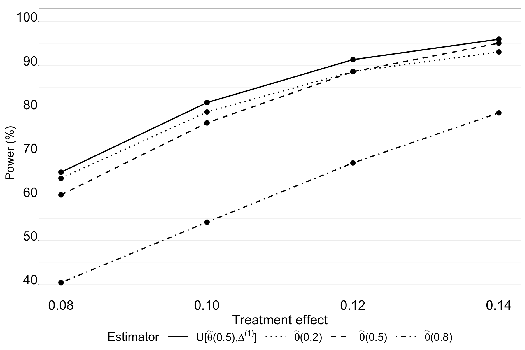
In terms of hypothesis testing to detect a promising treatment effect, we plot the power of rejecting the one-sided null hypothesis at a type I error rate under and varying treatment effect in Figure 2. The critical values of rejecting are computed at for our method, for , for , and for by the grid search method to control validating type I error rates not exceeding when . Our proposed method has a consistently higher power of detecting a promising treatment effect than the other three estimators. A more ethical and efficient adaptive clinical trial can be designed based on our proposed method to evaluate treatment options to cure COVID-19.
| Relative efficiency versus | |||||||||
|---|---|---|---|---|---|---|---|---|---|
| Bias | Root of MSE | ||||||||
| 0.47 | 0.47 | 0 | 0.001 | 0.039 | 1.012 | 1.164 | 2.154 | ||
| 0.57 | 0.1 | 0.001 | 0.045 | 1.195 | 1.035 | 1.621 | |||
| 0.59 | 0.12 | 0.001 | 0.047 | 1.286 | 1.018 | 1.484 | |||
| 0.61 | 0.14 | 0.050 | 1.383 | 1.007 | 1.355 | ||||
7 Discussion
In this article, we develop our ensemble framework by combining two base estimators with a linear formulation in (1). An alternative approach is to directly train DNN with base estimators as input to minimize MSE. As compared with this alternative, our proposed method has tractable MSE studied in Theorem 1 and conditions of achieving MSE reduction in Corollary 1. Moreover, our method has a small bias when combining two unbiased base estimators, with the upper bound studied in Theorem 2 in the Supplemental Materials and simulation results in Table 3. In addition to a reduced MSE, a smaller bias is also important for point estimation to more accurately estimate the parameter of interest, especially for the Adaptive COVID-19 Treatment Trial in Section 6.
Our proposed framework is general, in the sense that DNN can be replaced by other prediction models, for example, Support Vector Machine (SVM) or Random Forest (RF). The approximation error in Proposition 2 and the estimation error in (8) can be updated by corresponding results. As shown in Supplemental Table 4, DNN has a better performance than SVM and RF when estimating quantiles of scale-uniform distribution. In practice, one can implement our framework with different models and select the best one for a particular problem. With modified combination weight in (2) to accommodate different objectives, our automatic framework can be widely applied to many statistical problems, for example, variable selection with high dimensional data. Even in scenarios with limited improvement, the ensemble estimator is still meaningful in confirming that the base estimators have satisfactory performance.
There are some potential limitations of our method. The deep learning based approach requires additional training and computational time to obtain the estimator. However, as illustrated in our shared code, one can instantly compute the weight parameter based on well-trained neural networks and construct the ensemble estimator. Our method is currently under a parametric framework, such that the sampling distribution is known in Figure 1. Future works include generalization to nonparametric settings, and making statistical inference of the parameter of interest based on the proposed estimator.
Supplemental Materials
Supplementary Materials including Appendices, Tables and Figures referenced in this article are available online. The R code and a help file to replicate results in the main article are available at https://github.com/tian-yu-zhan/DNN_Point_Estimation.
Acknowledgements
The authors thank the editorial board and reviewers for their constructive comments.
This manuscript was supported by AbbVie Inc. AbbVie participated in the review and approval of the content. Tianyu Zhan is employed by AbbVie Inc., Haoda Fu is employed by Eli Lilly and Company, and Jian Kang is Professor in the Department of Biostatistics at the University of Michigan, Ann Arbor. Kang’s research was partially supported by NIH R01 GM124061 and R01 MH105561. All authors may own AbbVie stock.
Conflict of Interest
No potential competing interest was reported by the authors.
References
- Allaire and Chollet (2020) Allaire, J. and F. Chollet (2020). keras: R Interface to ’Keras’. R package version 2.2.5.0. https://keras.rstudio.com.
- Amemiya (1973) Amemiya, T. (1973). Regression analysis when the variance of the dependent variable is proportional to the square of its expectation. Journal of the American Statistical Association 68(344), 928–934.
- Anthony and Bartlett (2009) Anthony, M. and P. L. Bartlett (2009). Neural network learning: Theoretical foundations. Cambridge University Press.
- Bach (2017) Bach, F. (2017). Breaking the curse of dimensionality with convex neural networks. The Journal of Machine Learning Research 18(1), 629–681.
- Bauer et al. (2019) Bauer, B., M. Kohler, et al. (2019). On deep learning as a remedy for the curse of dimensionality in nonparametric regression. Annals of Statistics 47(4), 2261–2285.
- Boser et al. (1992) Boser, B. E., I. M. Guyon, and V. N. Vapnik (1992). A training algorithm for optimal margin classifiers. In Proceedings of the fifth annual workshop on Computational learning theory, pp. 144–152.
- Bretz et al. (2009) Bretz, F., F. Koenig, W. Brannath, E. Glimm, and M. Posch (2009). Adaptive designs for confirmatory clinical trials. Statistics in Medicine 28(8), 1181–1217.
- Chen et al. (2010) Chen, M.-H., D. K. Dey, P. Müller, D. Sun, and K. Ye (2010). Bayesian clinical trials. Frontiers of Statistical Decision Making and Bayesian Analysis, 257–284.
- Chen et al. (2014) Chen, M.-H., J. G. Ibrahim, D. Zeng, K. Hu, and C. Jia (2014). Bayesian design of superiority clinical trials for recurrent events data with applications to bleeding and transfusion events in myelodyplastic syndrome. Biometrics 70(4), 1003–1013.
- Chen and Guestrin (2016) Chen, T. and C. Guestrin (2016). XGBoost: A scalable tree boosting system. Proceedings of the 22nd acm sigkdd international conference on knowledge discovery and data mining, 785–794.
- Efron (2012) Efron, B. (2012). Large-scale inference: empirical Bayes methods for estimation, testing, and prediction, Volume 1. Cambridge University Press.
- European Medicines Agency (2007) European Medicines Agency (2007). Reflection paper on methodological issues in confirmatory clinical trials planned with an adaptive design. EMEA.
- Evans (2010) Evans, L. C. (2010). Partial differential equations. American Mathematical Society.
- Fan et al. (2014) Fan, J., F. Han, and H. Liu (2014). Challenges of big data analysis. National Science Review 1(2), 293–314.
- Fan et al. (2018) Fan, J., H. Liu, Z. Wang, and Z. Yang (2018). Curse of heterogeneity: Computational barriers in sparse mixture models and phase retrieval. arXiv preprint arXiv:1808.06996.
- Food and Drug Administration (2019) Food and Drug Administration (2019). Adaptive design clinical trials for drugs and biologics guidance for industry. https://www.fda.gov/regulatory-information/search-fda-guidance-documents/adaptive-design-clinical-trials-drugs-and-biologics-guidance-industry.
- Galili and Meilijson (2016) Galili, T. and I. Meilijson (2016). An example of an improvable Rao-Blackwell improvement, inefficient maximum likelihood estimator, and unbiased generalized bayes estimator. The American Statistician 70(1), 108–113.
- Goodfellow et al. (2016) Goodfellow, I., Y. Bengio, and A. Courville (2016). Deep learning. MIT press.
- Ioannou et al. (2020) Ioannou, G. N., W. Tang, L. A. Beste, M. A. Tincopa, G. L. Su, T. Van, E. B. Tapper, A. G. Singal, J. Zhu, and A. K. Waljee (2020). Assessment of a deep learning model to predict hepatocellular carcinoma in patients with hepatitis c cirrhosis. JAMA network open 3(9), e2015626–e2015626.
- James and Stein (1992) James, W. and C. Stein (1992). Estimation with quadratic loss. Breakthroughs in Statistics, 443–460.
- Khan (2015) Khan, R. A. (2015). A remark on estimating the mean of a normal distribution with known coefficient of variation. Statistics 49(3), 705–710.
- Koenker (2005) Koenker, R. (2005). Quantile regression. Cambridge University Press.
- Lehmann and Casella (2006) Lehmann, E. L. and G. Casella (2006). Theory of point estimation. Springer Science & Business Media.
- Liu et al. (2020) Liu, L. Y.-F., Y. Liu, and H. Zhu (2020). Masked convolutional neural network for supervised learning problems. Stat 9(1), e290.
- National Institutes of Health (2020) National Institutes of Health (2020). NIH Clinical Trial Shows Remdesivir Accelerates Recovery from Advanced COVID-19 . https://www.niaid.nih.gov/news-events/nih-clinical-trial-shows-remdesivir-accelerates-recovery-advanced-covid-19.
- Neuenschwander et al. (2010) Neuenschwander, B., G. Capkun-Niggli, M. Branson, and D. J. Spiegelhalter (2010). Summarizing historical information on controls in clinical trials. Clinical Trials 7(1), 5–18.
- Schmidt-Hieber et al. (2020) Schmidt-Hieber, J. et al. (2020). Nonparametric regression using deep neural networks with ReLU activation function. Annals of Statistics 48(4), 1875–1897.
- Shen and Yu (2010) Shen, J. and H. Yu (2010). Efficient spectral sparse grid methods and applications to high-dimensional elliptic problems. SIAM Journal on Scientific Computing 32(6), 3228–3250.
- Shen (2001) Shen, L. (2001). An improved method of evaluating drug effect in a multiple dose clinical trial. Statistics in Medicine 20(13), 1913–1929.
- Stallard et al. (2008) Stallard, N., S. Todd, and J. Whitehead (2008). Estimation following selection of the largest of two normal means. Journal of Statistical Planning and Inference 138(6), 1629–1638.
- Tibshirani (1996) Tibshirani, R. (1996). Regression shrinkage and selection via the lasso. Journal of the Royal Statistical Society: Series B (Methodological) 58(1), 267–288.
- van der Laan et al. (2007) van der Laan, M. J., E. C. Polley, and A. E. Hubbard (2007). Super learner. Statistical applications in genetics and molecular biology 6(1).
- Varewyck et al. (2014) Varewyck, M., E. Goetghebeur, M. Eriksson, and S. Vansteelandt (2014). On shrinkage and model extrapolation in the evaluation of clinical center performance. Biostatistics 15(4), 651–664.
- Williams and Rasmussen (2006) Williams, C. K. and C. E. Rasmussen (2006). Gaussian processes for machine learning, Volume 2. MIT press Cambridge, MA.
- Yang et al. (2007) Yang, H.-J., B. P. Roe, and J. Zhu (2007). Studies of stability and robustness for artificial neural networks and boosted decision trees. Nuclear Instruments and Methods in Physics Research Section A: Accelerators, Spectrometers, Detectors and Associated Equipment 574(2), 342–349.
- Yarotsky (2017) Yarotsky, D. (2017). Error bounds for approximations with deep ReLU networks. Neural Networks 94, 103–114.