跳到论文正文
W Papers独立论文阅读器 arXiv:2105.06265 论文正文 计算阅读时间 · 0%
引用这篇论文根据当前论文元数据生成,正式投稿前建议核对。


License: arXiv.org perpetual non-exclusive license
arXiv:2105.06265v2 [hep-lat] 20 Jul 2021

Lattice simulation of (2+1)​D(2+1)D phonetic solitons and the Renormalization group

Sadataka Furui Affiliation: (Formerly) Graduate School of Science and Engineering, Teikyo University, Utsunomiya, 320 Japan Email: furui@umb.teikyo-u.ac.jp
August 11, 2026
Abstract

The outline of lattice simulations of (2+1)​D(2+1)D soliton-propagations in the background of Weyl spinors is presented. Clifford algebra is applied on Luescher’s domain decomposition method. The Clifford algebra shows that there are loop parts and interpolating surface parts in the Wilson’s lattice action.

We adopt the Migdal-Kadanoff prescription and the fixed point action in momentum space of Benfatto and Gallavotti, and shows a road map for simulating phonetic solitons in materials.

Detections of topological anomalies (APS index) in nondestructive testing are discussed.

Keywords: 
Renormalization group and APS Index and Nonlinear PDE and Soliton

I Introduction

Propagation of a soliton in backgrounds of fermions is an interesting problem. In nondestructive testing (NDT), convolutions of a ultrasonic wave and its time reversed (TR) wave were measured to find anomalies in materialsFDS20; DSP20.

In the study of many fermion system, Luttinger Luttinger63 constructed a model whose exact solutions was derived. Wilson and Fischer WF72 studied critical exponents of Ising-like X​YXY model, using the fixed point(FP) method.

Bell and Wilson BW74 studied nonlinear renormalzation group in 2 and 4 fermion interacting Hamiltonian system in momentum space. Phase transitions in gauge and spin-lattice systems were studied by Migdal Migdal75a; Migdal75b. KadanoffKadanoff77 studied lattice renormalization group and the FP phenomenology. Creutz Creutz80 reviewed the beta function of the Migdal-Kadanoff prescription, and Wilson’s lattice simulations Wilson71a; Wilson71b; Wilson74.

In order to study Dirac fermion systems with Fermi momentum pF=(2​π/L)​(nF+12)p_{F}=(2\pi/L)(n_{F}+\frac{1}{2}) where [0,L][0,L] is the domain of a fermion, Benfatto et al. Gallavotti85; BG90; BGM92; BGPS94; BG95 adopted the renormalization group method. They studied beta function of fermions and bosons in the renormalization group theory.

Gruzberg et al. GRV05 showed that in the Altland-Zirnbauer (AZ) symmetry classes D​I​I​IDIII AZ97, there is a TR symmetry unbroken but spin-rotation (SR) broken phase exists. Ryu et al.RML12 studied gravitational and electromagnetic thermal responses using the AZ symmetry classes. In order to analyze whether there is time reversal symmetric spin rotation broken phase exist in bounded fermion background, and whether topological anomaly in fermionic materials can be detected is our problem.

Atiyah and Singer defined an index Hirzebruch78 as the difference of number of zero modes with positive chirality n+n+ and that with negative chirality n−n-, for locally elliptic differential operator DD in a compact Riemann manifold.

The Atiyah-Patodi-Singer (APS) index theoremAPS75 gives a relation between the number of zero modes in a bounded manifold. Atiyah, Bott and Patodi ABP73 considered a heat expansions of the index in a bounded region and studied the difference of number of zero mode in t≥0t\geq 0 region and that in t<0t<0 region. t≥0t\geq 0 region that in t<0t<0 region on Riemann manifolds with boundaries.

I was interested in the APS index as I analyzed the (2+1)​D(2+1)D convolution of a ultrasonic non-linear wave propagating in a plane and its time reversed (TR) wave, which is used in non destructive testings (NDT) by Dos Santos’ groupDSP20.

Nonlinear partial differential equation of Khokhlov-Zaboltskaya (KhZa) has a soliton solution, whose evolution is defined by real variables, and adopted as a model of phonon propagations.

The ratio of the length at which a discontinuity is formed ls=c02/ϵ​ω​u0l_{s}=c_{0}^{2}/\epsilon\omega u_{0}, diffraction length ld=ω​a2/2​c0l_{d}=\omega a^{2}/2c_{0} define variables z=x/lsz=x/l_{s}, N=ls/ldN=l_{s}/l_{d}.

A solution V=u/u0V=u/u_{0}, where u0u_{0} is a characteristic amplitude, can be expressed by a series of Bessel functions,

V\displaystyle V =\displaystyle= ∑n=1∞2n​z​Jn​(n​z1+N2​z2​e​x​p​(−R21+N2​z2))\displaystyle\sum_{n=1}^{\infty}\frac{2}{nz}J_{n}(\frac{nz}{\sqrt{1+N^{2}z^{2}}}exp(-\frac{R^{2}}{1+N^{2}z^{2}}))
×sin⁡n⁡[θ+a​r​c​t​a​n​(N​z)−R2​N​z1+N2​z2]\displaystyle\times\sin n[\theta+arctan(Nz)-R^{2}\frac{Nz}{1+{N^{2}z^{2}}}]
Refer to caption
Figure 1: The contour of the convolution at N=0.5N=0.5 near boundaries of z=0z=0 and z=1z=1. Three Δ​z\Delta z dependence are compared. Δ​z=1/36\Delta z=1/36(blue), 1/481/48 (green) and 1/721/72 (red).

A 2​D2D convolution as a function of zz at N=0.5N=0.5, there are two negative points near the boundary of the Liouville region as shown in Fig.1. The logaithm of negative convolution has the positive imaginary part. It means that t≥0t\geq 0 region is stable and t<0t<0 region is unstable, and n+−n−=2n_{+}-n_{-}=2.

In order to preserve chiral symmetry on lattices, Bell and WilsonBW74 proposed the Fixed Point(FP) action. Luescher and WeiszLW85 defined improved lattice gauge action following the program of Symanzik. Its action consists of a trial action 𝒜⁡(𝐒){\mathcal{A}}({\bf S}) of coarse lattices and correction terms which are defined recursively. Chiral fermions were studied in GW81; Luescher98a; Luescher98b; Luescher03; NN93; DGHHN95; HN97; Neuberger97; Hasenfratz98; Niedermeyer99

The method was applied in two dimensional O⁡(3)​σO(3)\sigma model by Blatter et al.BBHN96. The partition function on a lattice is given in a form

Z=∫D​𝐒​e−β​𝒜​(𝐒),Z=\int D{\bf S}e^{-\beta{\mathcal{A}}({\bf S})},

where the action in the continuum is

𝒜c​o​n​t​(𝐒)=12​∫d2​x​∂μ𝐒⁡(x)⋅∂μ𝐒⁡(x).{\mathcal{A}}_{cont}({\bf S})=\frac{1}{2}\int d^{2}x\partial_{\mu}{\bf S}(x)\cdot\partial_{\mu}{\bf S}(x).

The structure of this article is as follows. In the Section II, we explain FP lattice actions in (2+1)​D(2+1)D. An explicit calculation of eigenvalues of Wilson loop of length less than or equal to 8​a8a is given. In the Section III. recursive renormalization group analysis of (2+1)​D(2+1)D lattices is explained. In the Section IV, application of Luescher’s action of unitary groups to the symplectic group C​ℓ1,3+C\ell_{1,3}^{+} is explained. Application of the renormalization group to the scaling problem in propagation of phonetic solitons are discussed in Sction V. In view of success of instanton picture in spin field theory, relations between the topological charge and instantons and perspective is given in Section VI.

II Fixed point lattice actions in (2+1)​D(2+1)D

II.1 Paths on one 2DD plane expanded by e1e_{1} and e2e_{2}

DeGrand et al. DGHHN95 adopted FP action in chirally symmetric lattice QCD simulations in 4​D4D. space-time using S​U​(3)SU(3) symmetric Lie groups. They decomposed the FP action SF​P​(V)S^{FP}(V) as

SF​P​(V)=m​i​nU​(S0​(U)+T⁡(U,V))=SF​P​(U0)+T⁡(U0,V)S^{FP}(V)=min_{U}(S_{0}(U)+T(U,V))=S^{FP}(U_{0})+T(U_{0},V)

where U0U_{0} is the fine configuration. S0​(U)S_{0}(U) is a selected sets of configutations and T⁡(U,V)T(U,V) is obtained from an average of coarse configurations which is called 𝐑{\bf R} and VV, The series of a configuration UU to U0U_{0} is chosen by reducing the lattice spacing by a factor of 2.

In this process we replace actions on quarks to actions of Weyl spinors represented by quaternions, and necessarily the FP actions changes to eigenvalues of configurations described by quaternions.

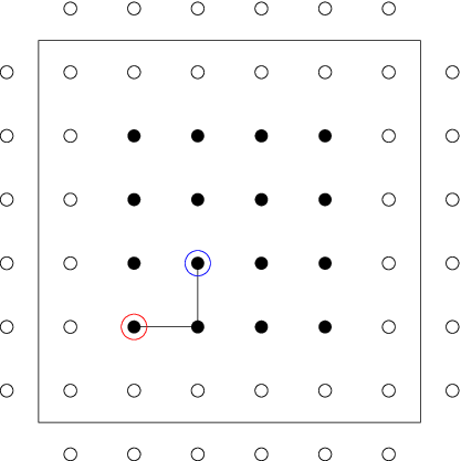
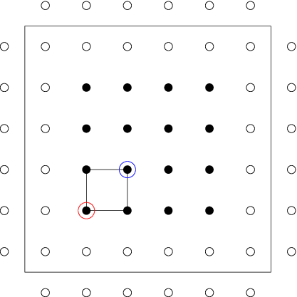
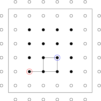
The Wilson loops that DeGrand et al. considered relevant to our (2+1)​D(2+1)D actions on a 2DD plane are shown in Fig.2, Fig.3 and Fig.4.

Refer to caption
Refer to caption
Figure 2: Loop1, Loop2 (left) and Loop5 (right). (Loop28 is a double path of Loop1.)
Refer to caption
Refer to caption
Figure 3: Loop6 (left) and Loop11 (right).
Refer to caption
Refer to caption
Figure 4: Loop12 (left) and Loop18 (right). ( Path orders of Loop5 and Loop12 are different.)

The Wilson loop plaquette calculation using the Clifford algebra can be performed as follows.

We define pure quaternions 𝐒∈𝐒3{\bf S}\in{\bf S}^{3} mapped from u=u1+−1​u2∈𝐂u=u_{1}+\sqrt{-1}u_{2}\in{\bf C} by

Si=2​ui1+|u|2(i=1,2),S0=1−|u|21+|u|2.\displaystyle{S}^{i}=\frac{2u_{i}}{1+|u|^{2}}\quad(i=1,2),\quad{S}^{0}=\frac{1-|u|^{2}}{1+|u|^{2}}.
𝐒=S1​e1+S2​e2+S0​e1∧e2.\displaystyle{\bf S}=S^{1}e_{1}+S^{2}e_{2}+S^{0}e_{1}\wedge e_{2}.

Here we use e1=(0110),e2=(0−−1−10)e_{1}=\left(\begin{array}[]{cc}0&1\\ 1&0\end{array}\right),\quad e_{2}=\left(\begin{array}[]{cc}0&-\sqrt{-1}\\ \sqrt{-1}&0\end{array}\right).

For a q∈𝐇q\in{\bf H}, taking a conjugation in 𝐂{\bf C} corresponds to taking a reversion, and we express it by q~\tilde{q}.

A mapping from a coordinate xx in the space 𝐑1,3{\bf R}^{1,3} is calculated by using X=(xx​x−Ix−)X=\left(\begin{array}[]{cc}x&xx^{-}\\ I&x^{-}\end{array}\right), where I=e0=(1001)I=e_{0}=\left(\begin{array}[]{cc}1&0\\ 0&1\end{array}\right) and the hyperplane reflection x→−x−x\to-x^{-} is represented by a multiplication of (01−10)\left(\begin{array}[]{cc}0&1\\ -1&0\end{array}\right).

e0−=−e0e_{0}^{-}=-e_{0}, e1−=(100−1)e_{1}^{-}=\left(\begin{array}[]{cc}1&0\\ 0&-1\end{array}\right) and e2−=(−100−1)e_{2}^{-}=\left(\begin{array}[]{cc}\sqrt{-1}&0\\ 0&\sqrt{-1}\end{array}\right).

A translation operator 𝒯=(Ic0I){\mathcal{T}}=\left(\begin{array}[]{cc}I&c\\ 0&I\end{array}\right), shifts the coordinate xx by cc Porteous95. The mapping X→YX\to Y is realized by

𝒯.X.𝒯−1=(x+c(x+c)​(x−−c)Ix−−c)=(yy​y−Iy−).{\mathcal{T}}.X.{\mathcal{T}}^{-1}=\left(\begin{array}[]{cc}x+c&(x+c)(x^{-}-c)\\ I&x^{-}-c\end{array}\right)=\left(\begin{array}[]{cc}y&yy^{-}\\ I&y^{-}\end{array}\right).

We define 𝒯(m,n)=(I(m​e1+n​e2)​a0I),{\mathcal{T}}_{(m,n)}=\left(\begin{array}[]{cc}I&(me_{1}+ne_{2})a\\ 0&I\end{array}\right), where aa is the lattice constant, and 𝒯(m,n)−1=𝒯(−m,−n){\mathcal{T}}^{-1}_{(m,n)}={\mathcal{T}}_{(-m,-n)}.

𝒯(m,n)​(x⁡(u1,u2)x​x−​(u1,u2)Ix−​(u1,u2))​𝒯(−m,−n){\mathcal{T}}_{(m,n)}\left(\begin{array}[]{cc}x(u_{1},u_{2})&xx^{-}(u_{1},u_{2})\\ I&x^{-}(u_{1},u_{2})\end{array}\right){\mathcal{T}}_{(-m,-n)}

agrees with

(x⁡(u1′,u2′)x​x−​(u1′,u2′)Ix−​(u1′,u2′))\quad\quad\left(\begin{array}[]{cc}x(u_{1}^{\prime},u_{2}^{\prime})&xx^{-}(u_{1}^{\prime},u_{2}^{\prime})\\ I&x^{-}(u_{1}^{\prime},u_{2}^{\prime})\end{array}\right)

where x⁡(u1′,u2′)x(u_{1}^{\prime},u_{2}^{\prime}) are x⁡(u1+m​a,u2+n​a)x(u_{1}+ma,u_{2}+na), up to linear order of aa.

Using a mapping of 𝐇{\bf H} to 𝐂{\bf C}, XX can be expressed as

X⁡(u1,u2)=\displaystyle X(u_{1},u_{2})=
(−1​u1u2−1​u12−u1​u2−u1​u2+−1​u22−u2−−1​u1−u1​u2−−1​u22−1​u12+u1​u210u1+−1​u20010u1+−1​u2)\displaystyle\left(\begin{array}[]{cccc}\sqrt{-1}u_{1}&u_{2}&\sqrt{-1}u_{1}^{2}-u_{1}u_{2}&-u_{1}u_{2}+\sqrt{-1}u_{2}^{2}\\ -u_{2}&-\sqrt{-1}u_{1}&-u_{1}u_{2}-\sqrt{-1}u_{2}^{2}&\sqrt{-1}u_{1}^{2}+u_{1}u_{2}\\ 1&0&u_{1}+\sqrt{-1}u_{2}&0\\ 0&1&0&u_{1}+\sqrt{-1}u_{2}\end{array}\right)

We calculate the product 𝒯(m,n)​X​(u1,u2)​𝒯(−m,−n){\mathcal{T}}_{(m,n)}X(u_{1},u_{2}){\mathcal{T}}_{(-m,-n)} using MathematicaMathematica and obtain the link matrix that that operates on quaternions sitting at (u1,u2)(u_{1},u_{2}) to another quaternion.

We define ∂1𝐒⁡[u1,u2]\partial_{1}{\bf S}[u_{1},u_{2}] as

d​𝐒1​[u1,u2]=(𝒯(1,0)​X​(u1,u2)​𝒯(−1,−0)−X⁡(u1,u2))/a.,d{\bf S}_{1}[u_{1},u_{2}]=({\mathcal{T}}_{(1,0)}X(u_{1},u_{2}){\mathcal{T}}_{(-1,-0)}-X(u_{1},u_{2}))/a.,

and ∂2𝐒⁡[u1,u2]\partial_{2}{\bf S}[u_{1},u_{2}] as

d​𝐒2​[u1,u2]=(𝒯(0,1)​X​(u1,u2)​𝒯(−0,−1)−X⁡(u1,u2))/a.d{\bf S}_{2}[u_{1},u_{2}]=({\mathcal{T}}_{(0,1)}X(u_{1},u_{2}){\mathcal{T}}_{(-0,-1)}-X(u_{1},u_{2}))/a.

If the linked quaternion is separated by a​e1ae_{1}, the matrix element is denoted as t​1​[a,u1,u2]i​jt1[a,u_{1},u_{2}]_{ij} (1≤i,j≤41\leq i,j\leq 4).

t​1​[a,u1,u2]11=−1​(a+2​u11+u12+u22),\displaystyle t1[a,u_{1},u_{2}]_{11}=\sqrt{-1}(a+\frac{2u_{1}}{1+u_{1}^{2}+u_{2}^{2}}),
t​1​[a,u1,u2]12=−−1​(u12+(−1+u2)2)1+u12+u22,\displaystyle t1[a,u_{1},u_{2}]_{12}=-\frac{\sqrt{-1}(u_{1}^{2}+(\sqrt{-1}+u_{2})^{2})}{1+u_{1}^{2}+u_{2}^{2}},
t​1​[a,u1,u2]13=1(1+u12+u22)2\displaystyle t1[a,u_{1},u_{2}]_{13}=\frac{1}{(1+u_{1}^{2}+u_{2}^{2})^{2}}
×(−8​−1​u1​u2+a⁡(1+u12+u22)​(u12+(−−1+u2)2)CLOSE\displaystyle\times(-8\sqrt{-1}u_{1}u_{2}+a(1+u_{1}^{2}+u_{2}^{2})(u_{1}^{2}+(-\sqrt{-1}+u_{2})^{2})
OPEN+a⁡(1+u12+u22)​(2​u1+a⁡(1+u12+u22))),\displaystyle+a(1+u_{1}^{2}+u_{2}^{2})(2u_{1}+a(1+u_{1}^{2}+u_{2}^{2}))),
t​1​[a,u1,u2]14=1(1+u12+u22)2​(u14+(−1+u2)4CLOSE\displaystyle t1[a,u_{1},u_{2}]_{14}=\frac{1}{(1+u_{1}^{2}+u_{2}^{2})^{2}}(u_{1}^{4}+(\sqrt{-1}+u_{2})^{4}
+2​a​u1​(1+u12+u22)+2​u12​(1+2​−1​u2+u22)\displaystyle+2au_{1}(1+u_{1}^{2}+u_{2}^{2})+2u_{1}^{2}(1+2\sqrt{-1}u_{2}+u_{2}^{2})
OPEN+a⁡(1+u12+u22)​(u12+(−1+u2)2)),\displaystyle+a(1+u_{1}^{2}+u_{2}^{2})(u_{1}^{2}+(\sqrt{-1}+u_{2})^{2})),
t​1​[a,u1,u2]21=−−1​(u12+(−−1+u2)2)1+u12+u22,\displaystyle t1[a,u_{1},u_{2}]_{21}=-\frac{\sqrt{-1}(u_{1}^{2}+(-\sqrt{-1}+u_{2})^{2})}{1+u_{1}^{2}+u_{2}^{2}},
t​1​[a,u1,u2]22=−−1​(a+2​u11+u12+u22),\displaystyle t1[a,u_{1},u_{2}]_{22}=-\sqrt{-1}(a+\frac{2u_{1}}{1+u_{1}^{2}+u_{2}^{2}}),
t​1​[a,u1,u2]23=−1(1+u12+u22)2\displaystyle t1[a,u_{1},u_{2}]_{23}=-\frac{1}{(1+u_{1}^{2}+u_{2}^{2})^{2}}
×(u14+(−−1+u2)4+2​a​u1​(1+u12+u22)CLOSE\displaystyle\times(u_{1}^{4}+(-\sqrt{-1}+u_{2})^{4}+2au_{1}(1+u_{1}^{2}+u_{2}^{2})
+2​u12​(1−2​−1​u2+u22)\displaystyle+2u_{1}^{2}(1-2\sqrt{-1}u_{2}+u_{2}^{2})
OPEN+a⁡(1+u12+u22)​(u12+(−−1+u2)2)),\displaystyle+a(1+u_{1}^{2}+u_{2}^{2})(u_{1}^{2}+(-\sqrt{-1}+u_{2})^{2})),
t​1​[a,u1,u2]24=1(1+u12+u22)2\displaystyle t1[a,u_{1},u_{2}]_{24}=\frac{1}{(1+u_{1}^{2}+u_{2}^{2})^{2}}
×(8​−1​u1​u2+a⁡(1+u12+u22)​(u12+(−1+u2)2)CLOSE\displaystyle\times(8\sqrt{-1}u_{1}u_{2}+a(1+u_{1}^{2}+u_{2}^{2})(u_{1}^{2}+(\sqrt{-1}+u_{2})^{2})
OPEN+a⁡(1+u12+u22)​(2​u1+a⁡(1+u12+u22))),\displaystyle+a(1+u_{1}^{2}+u_{2}^{2})(2u_{1}+a(1+u_{1}^{2}+u_{2}^{2}))),
t​1​[a,u1,u2]31=1,\displaystyle t1[a,u_{1},u_{2}]_{31}=1,
t​1​[a,u1,u2]32=0,\displaystyle t1[a,u_{1},u_{2}]_{32}=0,
t​1​[a,u1,u2]33=−−1​(a+u12+(−−1+u2)21+u12+u22),\displaystyle t1[a,u_{1},u_{2}]_{33}=-\sqrt{-1}(a+\frac{u_{1}^{2}+(-\sqrt{-1}+u_{2})^{2}}{1+u_{1}^{2}+u_{2}^{2}}),
t​1​[a,u1,u2]34=−2​−1​u11+u12+u22,\displaystyle t1[a,u_{1},u_{2}]_{34}=-\frac{2\sqrt{-1}u_{1}}{1+u_{1}^{2}+u_{2}^{2}},
t​1​[a,u1,u2]41=0,\displaystyle t1[a,u_{1},u_{2}]_{41}=0,
t​1​[a,u1,u2]42=1,\displaystyle t1[a,u_{1},u_{2}]_{42}=1,
t​1​[a,u1,u2]43=−2​−1​u11+u12+u22,\displaystyle t1[a,u_{1},u_{2}]_{43}=-\frac{2\sqrt{-1}u_{1}}{1+u_{1}^{2}+u_{2}^{2}},
t​1​[a,u1,u2]44=−1​(a+(u12+(−1+u2)2CLOSE1+u12+u22).\displaystyle t1[a,u_{1},u_{2}]_{44}=\sqrt{-1}(a+\frac{(u_{1}^{2}+(\sqrt{-1}+u_{2})^{2}}{1+u_{1}^{2}+u_{2}^{2}}).

Similarly link to another quaternion separated by b​e2be_{2} is represented by

t​2​[b,u1,u2]11=2​−1​u11+u12+u22,\displaystyle t2[b,u_{1},u_{2}]_{11}=\frac{2\sqrt{-1}u_{1}}{1+u_{1}^{2}+u_{2}^{2}},
t​2​[b,u1,u2]12=b−−1​u12+(−1+u2)21+u12+u22,\displaystyle t2[b,u_{1},u_{2}]_{12}=b-\sqrt{-1}\frac{u_{1}^{2}+(\sqrt{-1}+u_{2})^{2}}{1+u_{1}^{2}+u_{2}^{2}},
t​2​[b,u1,u2]13=b2−8​−1​u1​u2(1+u12+u22)2\displaystyle t2[b,u_{1},u_{2}]_{13}=b^{2}-\frac{8\sqrt{-1}u_{1}u_{2}}{(1+u_{1}^{2}+u_{2}^{2})^{2}}
−−1​b​(2​u1+u12+(−1+u2)2)1+u12+u22,\displaystyle-\frac{\sqrt{-1}b(2u_{1}+u_{1}^{2}+(\sqrt{-1}+u_{2})^{2})}{1+u_{1}^{2}+u_{2}^{2}},
t​2​[b,u1,u2]14=1(1+u12+u22)2\displaystyle t2[b,u_{1},u_{2}]_{14}=\frac{1}{(1+u_{1}^{2}+u_{2}^{2})^{2}}
×(u14+(−1+u2)4−2​−1​b​u1​(1+u12+u22)CLOSE\displaystyle\times(u_{1}^{4}+(\sqrt{-1}+u_{2})^{4}-2\sqrt{-1}bu_{1}(1+u_{1}^{2}+u_{2}^{2})
+2​u12​(1+2​−1​u2+u22)\displaystyle+2u_{1}^{2}(1+2\sqrt{-1}u_{2}+u_{2}^{2})
OPEN+−1​b​(1+u12+u22)​(u12+(−1+u2)2)),\displaystyle+\sqrt{-1}b(1+u_{1}^{2}+u_{2}^{2})(u_{1}^{2}+(\sqrt{-1}+u_{2})^{2})),
t​2​[b,u1,u2]21=−b−−1​(u12+(−−1+u2)2)1+u12+u22,\displaystyle t2[b,u_{1},u_{2}]_{21}=-b-\frac{\sqrt{-1}(u_{1}^{2}+(-\sqrt{-1}+u_{2})^{2})}{1+u_{1}^{2}+u_{2}^{2}},
t​2​[b,u1,u2]22=−2​−1​u11+u12+u22,\displaystyle t2[b,u_{1},u_{2}]_{22}=-\frac{2\sqrt{-1}u_{1}}{1+u_{1}^{2}+u_{2}^{2}},
t​2​[b,u1,u2]23=−1(1+u12+u22)2\displaystyle t2[b,u_{1},u_{2}]_{23}=-\frac{1}{(1+u_{1}^{2}+u_{2}^{2})^{2}}
×(u14+(−−1+u2)4+2​−1​b​u1​(1+u12+u22)CLOSE\displaystyle\times(u_{1}^{4}+(-\sqrt{-1}+u_{2})^{4}+2\sqrt{-1}bu_{1}(1+u_{1}^{2}+u_{2}^{2})
+2​u12​(1−2​−1​u2+u22)\displaystyle+2u_{1}^{2}(1-2\sqrt{-1}u_{2}+u_{2}^{2})
OPEN−−1​b​(1+u12+u22)​(u12+(−−1+u2)2)),\displaystyle-\sqrt{-1}b(1+u_{1}^{2}+u_{2}^{2})(u_{1}^{2}+(-\sqrt{-1}+u_{2})^{2})),
t​2​[b,u1,u2]24=1(1+u12+u22)2\displaystyle t2[b,u_{1},u_{2}]_{24}=\frac{1}{(1+u_{1}^{2}+u_{2}^{2})^{2}}
×(8​−1​u1​u2+2​−1​b​u1​(1+u12+u22)CLOSE\displaystyle\times(8\sqrt{-1}u_{1}u_{2}+2\sqrt{-1}bu_{1}(1+u_{1}^{2}+u_{2}^{2})
+b⁡(1+u12+u22)​(b⁡(1+u12+u22)CLOSE\displaystyle+b(1+u_{1}^{2}+u_{2}^{2})(b(1+u_{1}^{2}+u_{2}^{2})
OPENOPEN+−1​(u12+(−−1+u2)2))),\displaystyle+\sqrt{-1}(u_{1}^{2}+(-\sqrt{-1}+u_{2})^{2}))),
t​2​[b,u1,u2]31=1,\displaystyle t2[b,u_{1},u_{2}]_{31}=1,
t​2​[b,u1,u2]32=0,\displaystyle t2[b,u_{1},u_{2}]_{32}=0,
t​2​[b,u1,u2]33=−−1​(u12+(−−1+u2)2)1+u12+u22,\displaystyle t2[b,u_{1},u_{2}]_{33}=-\frac{\sqrt{-1}(u_{1}^{2}+(-\sqrt{-1}+u_{2})^{2})}{1+u_{1}^{2}+u_{2}^{2}},
t​2​[b,u1,u2]34=−b−2​−1​u11+u12+u22,\displaystyle t2[b,u_{1},u_{2}]_{34}=-b-\frac{2\sqrt{-1}u_{1}}{1+u_{1}^{2}+u_{2}^{2}},
t​2​[b,u1,u2]41=0,\displaystyle t2[b,u_{1},u_{2}]_{41}=0,
t​2​[b,u1,u2]42=1,\displaystyle t2[b,u_{1},u_{2}]_{42}=1,
t​2​[b,u1,u2]43=b−2​−1​u11+u12+u22,\displaystyle t2[b,u_{1},u_{2}]_{43}=b-\frac{2\sqrt{-1}u_{1}}{1+u_{1}^{2}+u_{2}^{2}},
t​2​[b,u1,u2]44=−1​(u12+(−1+u2)2)1+u12+u22.\displaystyle t2[b,u_{1},u_{2}]_{44}=\frac{\sqrt{-1}(u_{1}^{2}+(\sqrt{-1}+u_{2})^{2})}{1+u_{1}^{2}+u_{2}^{2}}.

For the Loop1, we multiply matrices

L​1​[u1,u2]=t​2​[−14,u1,u2+14]×t​1​[−14,u1+14,u2+14]\displaystyle L1[u_{1},u_{2}]=t2[-\frac{1}{4},u_{1},u_{2}+\frac{1}{4}]\times t1[-\frac{1}{4},u_{1}+\frac{1}{4},u_{2}+\frac{1}{4}]
×t​2​[14,u1+14,u2]×t​1​[14,u1,u2].\displaystyle\times t2[\frac{1}{4},u_{1}+\frac{1}{4},u_{2}]\times t1[\frac{1}{4},u_{1},u_{2}].

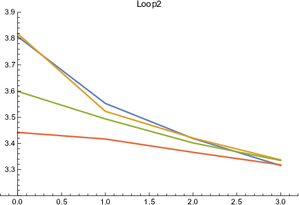
The absolute value of the eigenvalues of d​𝐒​[0,i]d{\bf S}[0,i] (Blue),d​𝐒​[1,i]d{\bf S}[1,i] (Orange),d​𝐒​[2,i]d{\bf S}[2,i] (Green), d​𝐒​[3,i]d{\bf S}[3,i] (Red) for i=0,1,2,3i=0,1,2,3 are plotted in Fig,5. The similar figures are shown in the following loops.

Refer to caption
Figure 5: The absolute value of eigenvalues in Loop1 for a fixed u1u_{1} as a function of u2u_{2}. (Δ​ui=1\Delta u_{i}=1 (i=1,2)(i=1,2))

For the Loop 2

L​2​[u1,u2]=t​2​[−12,u1,u2+12]×t​1​[−14,u1+14,u2+12]\displaystyle L2[u_{1},u_{2}]=t2[-\frac{1}{2},u_{1},u_{2}+\frac{1}{2}]\times t1[-\frac{1}{4},u_{1}+\frac{1}{4},u_{2}+\frac{1}{2}]
×t​2​[12,u1+14,u2]×t​1​[14,u1,u2].\displaystyle\times t2[\frac{1}{2},u_{1}+\frac{1}{4},u_{2}]\times t1[\frac{1}{4},u_{1},u_{2}].
Refer to caption
Figure 6: The absolute value of eigenvalues in Loop2 for a fixed u1u_{1} as a function of u2u_{2}. (Δ​ui=1\Delta u_{i}=1 (i=1,2)(i=1,2))

For the Loop5

L​5​[u1,u2]=t​2​[−14,u1,u2+14]×t​1​[−14,u1,u2+14]\displaystyle L5[u_{1},u_{2}]=t2[-\frac{1}{4},u_{1},u_{2}+\frac{1}{4}]\times t1[-\frac{1}{4},u_{1},u_{2}+\frac{1}{4}]
×t​2​[−14,u1+14,u2+14]×t​1​[−14,u1+14,u2+12]\displaystyle\times t2[-\frac{1}{4},u_{1}+\frac{1}{4},u_{2}+\frac{1}{4}]\times t1[-\frac{1}{4},u_{1}+\frac{1}{4},u_{2}+\frac{1}{2}]
×t​2​[14,u1+12,u2+12]×t​1​[14,u1+14,u2+14]\displaystyle\times t2[\frac{1}{4},u_{1}+\frac{1}{2},u_{2}+\frac{1}{2}]\times t1[\frac{1}{4},u_{1}+\frac{1}{4},u_{2}+\frac{1}{4}]
×t​2​[14,u1+14,u2]×t​1​[14,u1,u2].\displaystyle\times t2[\frac{1}{4},u_{1}+\frac{1}{4},u_{2}]\times t1[\frac{1}{4},u_{1},u_{2}].
Refer to caption
Figure 7: The absolute value of eigenvalues in Loop5 for a fixed u1u_{1} as a function of u2u_{2}. (Δ​ui=1\Delta u_{i}=1 (i=1,2)(i=1,2))

For the Loop 6

L​6​[u1,u2]=t​2​[−12,u1,u2+12]×t​1​[−12,u1+12,u2+12]\displaystyle L6[u_{1},u_{2}]=t2[-\frac{1}{2},u_{1},u_{2}+\frac{1}{2}]\times t1[-\frac{1}{2},u_{1}+\frac{1}{2},u_{2}+\frac{1}{2}]
×t​2​[14,u1+12,u2+14]×t​1​[14,u1+14,u2+14]\displaystyle\times t2[\frac{1}{4},u_{1}+\frac{1}{2},u_{2}+\frac{1}{4}]\times t1[\frac{1}{4},u_{1}+\frac{1}{4},u_{2}+\frac{1}{4}]
×t​2​[14,u1+14,u2]×t​1​[14,u1,u2].\displaystyle\times t2[\frac{1}{4},u_{1}+\frac{1}{4},u_{2}]\times t1[\frac{1}{4},u_{1},u_{2}].
Refer to caption
Figure 8: The absolute value of eigenvalues in Loop6 for a fixed u1u_{1} as a function of u2u_{2}. (Δ​ui=1\Delta u_{i}=1 (i=1,2)(i=1,2)) .

For the Loop11

L​11​[u1,u2]=t​2​[−14,u1,u2+14]×t​1​[−14,u1+14,u2+14]\displaystyle L11[u_{1},u_{2}]=t2[-\frac{1}{4},u_{1},u_{2}+\frac{1}{4}]\times t1[-\frac{1}{4},u_{1}+\frac{1}{4},u_{2}+\frac{1}{4}]
×t​2​[14,u1+14,u2]×t​1​[−14,u1+12,u2]\displaystyle\times t2[\frac{1}{4},u_{1}+\frac{1}{4},u_{2}]\times t1[-\frac{1}{4},u_{1}+\frac{1}{2},u_{2}]
×t​2​[−14,u1+12,u2+14]×t​1​[14,u1+14,u2+14]\displaystyle\times t2[-\frac{1}{4},u_{1}+\frac{1}{2},u_{2}+\frac{1}{4}]\times t1[\frac{1}{4},u_{1}+\frac{1}{4},u_{2}+\frac{1}{4}]
×t​2​[14,u1+14,u2]×t​1​[14,u1,u2].\displaystyle\times t2[\frac{1}{4},u_{1}+\frac{1}{4},u_{2}]\times t1[\frac{1}{4},u_{1},u_{2}].
Refer to caption
Figure 9: The absolute value of eigenvalues in Loop11 for a fixed u1u_{1} as a function of u2u_{2}. (Δ​ui=1\Delta u_{i}=1 (i=1,2)(i=1,2)).

For the Loop12

L​12​[u1,u2]=t​2​[−14,u1,u2+14]×t​1​[−12,u1+12,u2+14]\displaystyle L12[u_{1},u_{2}]=t2[-\frac{1}{4},u_{1},u_{2}+\frac{1}{4}]\times t1[-\frac{1}{2},u_{1}+\frac{1}{2},u_{2}+\frac{1}{4}]
×t​2​[−14,u1+12,u2+12]×t​1​[14,u1+14,u2+12]\displaystyle\times t2[-\frac{1}{4},u_{1}+\frac{1}{2},u_{2}+\frac{1}{2}]\times t1[\frac{1}{4},u_{1}+\frac{1}{4},u_{2}+\frac{1}{2}]
×t​2​[12,u1+14,u2]×t​1​[14,u1,u2].\displaystyle\times t2[\frac{1}{2},u_{1}+\frac{1}{4},u_{2}]\times t1[\frac{1}{4},u_{1},u_{2}].
Refer to caption
Figure 10: The absolute value of eigenvalues in Loop12 for a fixed u1u_{1} as a function of u2u_{2}. (Δ​ui=1\Delta u_{i}=1 (i=1,2)(i=1,2))

For the Loop18

L​18​[u1,u2]=t​2​[−12,u1,u2+12]×t​1​[−12,u1+12,u2+12]\displaystyle L18[u_{1},u_{2}]=t2[-\frac{1}{2},u_{1},u_{2}+\frac{1}{2}]\times t1[-\frac{1}{2},u_{1}+\frac{1}{2},u_{2}+\frac{1}{2}]
×t​2​[12,u1+12,u2]×t​1​[12,u1,u2].\displaystyle\times t2[\frac{1}{2},u_{1}+\frac{1}{2},u_{2}]\times t1[\frac{1}{2},u_{1},u_{2}].
Refer to caption
Figure 11: The absolute value of eigenvalues in Loop18 for a fixed u1u_{1} as a function of u2u_{2}. (Δ​ui=1\Delta u_{i}=1 (i=1,2)(i=1,2))

For the Loop28

L​28​[u1,u2]=t​2​[−14,u1,u2+14]×t​1​[−14,u1+14,u2+14]\displaystyle L28[u_{1},u_{2}]=t2[-\frac{1}{4},u_{1},u_{2}+\frac{1}{4}]\times t1[-\frac{1}{4},u_{1}+\frac{1}{4},u_{2}+\frac{1}{4}]
×t​2​[14,u1+14,u2]×t​1​[14,u1,u2]\displaystyle\times t2[\frac{1}{4},u_{1}+\frac{1}{4},u_{2}]\times t1[\frac{1}{4},u_{1},u_{2}]
×t​2​[−14,u1,u2+14]×t​1​[−14,u1+14,u2+14]\displaystyle\times t2[-\frac{1}{4},u_{1},u_{2}+\frac{1}{4}]\times t1[-\frac{1}{4},u_{1}+\frac{1}{4},u_{2}+\frac{1}{4}]
×t​2​[14,u1+14,u2]×t​1​[14,u1,u2].\displaystyle\times t2[\frac{1}{4},u_{1}+\frac{1}{4},u_{2}]\times t1[\frac{1}{4},u_{1},u_{2}].
Refer to caption
Figure 12: The absolute value of eigenvalues in Loop28 for a fixed u1u_{1} as a function of u2u_{2}. (Δ​ui=1\Delta u_{i}=1 (i=1,2)(i=1,2))

The eigen-quatrnions give the fixed point on the manifold.

As an example the 2×22\times 2 matrix at left-down corner of the 4×44\times 4 matrix of L​1​[0,0]L1[0,0] has the eigenvalue

χ⁡(L​1​[0,0])=1.98353±2.62338​−1\chi(L1[0,0])=1.98353\pm 2.62338\sqrt{-1}

and the eigen-quaternion

𝐒⁡(L​1​[0,0])\displaystyle{\bf S}(L1[0,0])
=\displaystyle= (0.974730.20534+0.087986​−1−0.20534+0.087986​−10.97473)\displaystyle\left(\begin{array}[]{cc}0.97473&0.20534+0.087986\sqrt{-1}\\ -0.20534+0.087986\sqrt{-1}&0.97473\end{array}\right)
=\displaystyle= 0.97473​e0+0.20534​e2+0.087986​e1∧e2.\displaystyle 0.97473e_{0}+0.20534e_{2}+0.087986e_{1}\wedge e_{2}.

Although the path is on a 2​D2D plane, the eigenvector has the e1∧e2e_{1}\wedge e_{2} component.

When u1u_{1} and u2u_{2} are large, convergence of eigenvalues can be seen. When a path intersects to its own path, the convergence at large u12+u22{u_{1}}^{2}+{u_{2}}^{2} is not strong.

Along the path L​1​[0,0]L1[0,0],

d​𝐒​(L​1​[0,0])=d​S1​[0,0]+d​S2​[14,0]−d​S1​[14,14]−d​S2​[0,14]d{\bf S}(L1[0,0])=dS_{1}[0,0]+dS_{2}[\frac{1}{4},0]-dS_{1}[\frac{1}{4},\frac{1}{4}]-dS_{2}[0,\frac{1}{4}]

has a non-zero quaternion element in the right-upper corner of the 4×44\times 4 matrix.,

(−1.13725−0.02614​−1−0.19608−0.91503​−10.19608−0.91503​−1−1.13725+0.02614​−1)\displaystyle\left(\begin{array}[]{cc}-1.13725-0.02614\sqrt{-1}&-0.19608-0.91503\sqrt{-1}\\ 0.19608-0.91503\sqrt{-1}&-1.13725+0.02614\sqrt{-1}\end{array}\right)
=\displaystyle= −1.13725​e0−0.02614​e1−0.19608​e2−0.91503​e1∧e2,\displaystyle-1.13725e_{0}-0.02614e_{1}-0.19608e_{2}-0.91503e_{1}\wedge e_{2},

and the other elements are zero.

There are 9 configurations of d​𝐒​(L​1​[ui,uj])d{\bf S}(L1[u_{i},u_{j}]), (0≤i/4,j/4≤1)(0\leq i/4,j/4\leq 1).

In the case of Loop18, whose length of the side is twice as that of Loop1,

χ⁡(L​18​[0,0])=2.31556±2.87632​−1\chi(L18[0,0])=2.31556\pm 2.87632\sqrt{-1}

and the eigen-quaternion

𝐒⁡(L​18​[0,0])\displaystyle{\bf S}(L18[0,0])
=\displaystyle= (0.25767+0.14704​−10.954980.95498−0.25767+0.14704​−1)\displaystyle\left(\begin{array}[]{cc}0.25767+0.14704\sqrt{-1}&0.95498\\ 0.95498&-0.25767+0.14704\sqrt{-1}\end{array}\right)
=\displaystyle= 0.14704​−1​e0−0.25267​−1​e1−0.95498​−1​e1∧e2,\displaystyle 0.14704\sqrt{-1}e_{0}-0.25267\sqrt{-1}e_{1}-0.95498\sqrt{-1}e_{1}\wedge e_{2},
d​𝐒​(L​18​[0,0])=d​S1​[0,0]+d​S2​[12,0]−d​S1​[12,12]−d​S2​[0,12]d{\bf S}(L18[0,0])=dS_{1}[0,0]+dS_{2}[\frac{1}{2},0]-dS_{1}[\frac{1}{2},\frac{1}{2}]-dS_{2}[0,\frac{1}{2}]

has the right-upper corner

(−2.13333−0.13333​−1−0.53333−1.46667​−10.53333−1.46667​−1−2.13333+0.13333​−1)\displaystyle\left(\begin{array}[]{cc}-2.13333-0.13333\sqrt{-1}&-0.53333-1.46667\sqrt{-1}\\ 0.53333-1.46667\sqrt{-1}&-2.13333+0.13333\sqrt{-1}\end{array}\right)
=\displaystyle= −2.1333​e0−0.13333​e1−0.53333​e2−1.46667​e1∧e2.\displaystyle-2.1333e_{0}-0.13333e_{1}-0.53333e_{2}-1.46667e_{1}\wedge e_{2}.

There are 4 configurations of d​𝐒​(L​18​[ui,uj])d{\bf S}(L18[u_{i},u_{j}]) (ui,uj)=(0,0),(12,0)(u_{i},u_{j})=(0,0),(\frac{1}{2},0),(14,14)(\frac{1}{4},\frac{1}{4}),(0,14)(0,\frac{1}{4}). The absolute value of the eigenvalues of L​18L18 are enhanced from that of L​1L1. Elements of eigen-quaternions of L​18L18 are multiplied by pure imaginary numbers to those of L​1L1.

II.2 Paths on two planes connected by e1∧e2e_{1}\wedge e_{2}

The paths containing e1∧e2e_{1}\wedge e_{2} components are analyzed similarly to that without containing the terms.

The link to another quaternion separated by c​e1∧e2ce_{1}\wedge e_{2} is represented by

t​3​[c,u1,u2]11=2​−1​u11+u12+u22,\displaystyle t3[c,u_{1},u_{2}]_{11}=\frac{2\sqrt{-1}u_{1}}{1+u_{1}^{2}+u_{2}^{2}},
t​3​[c,u1,u2]12=−1​(c−u12+(−1+u2)21+u12+u22),\displaystyle t3[c,u_{1},u_{2}]_{12}=\sqrt{-1}(c-\frac{u_{1}^{2}+(\sqrt{-1}+u_{2})^{2}}{1+u_{1}^{2}+u_{2}^{2}}),
t​3​[c,u1,u2]13=1(1+u12+u22)2\displaystyle t3[c,u_{1},u_{2}]_{13}=\frac{1}{(1+u_{1}^{2}+u_{2}^{2})^{2}}
×(−8​−1​u1​u2+2​c​u1​(1+u12+u22)CLOSE\displaystyle\times(-8\sqrt{-1}u_{1}u_{2}+2cu_{1}(1+u_{1}^{2}+u_{2}^{2})
−c⁡(1+u12+u22)​(u12+(−1+u2)2CLOSE\displaystyle-c(1+u_{1}^{2}+u_{2}^{2})(u_{1}^{2}+(\sqrt{-1}+u_{2})^{2}
OPENOPEN−c⁡(1+u12+u22))),\displaystyle-c(1+u_{1}^{2}+u_{2}^{2}))),
t​3​[c,u1,u2]14=1(1+u12+u22)2\displaystyle t3[c,u_{1},u_{2}]_{14}=\frac{1}{(1+u_{1}^{2}+u_{2}^{2})^{2}}
×(u14+(−1+u2)4+2​c​u1​(1+u12+u22)CLOSE\displaystyle\times(u_{1}^{4}+(\sqrt{-1}+u_{2})^{4}+2cu_{1}(1+u_{1}^{2}+u_{2}^{2})
+2​u12​(1+2​−1​u2+u22)\displaystyle+2u_{1}^{2}(1+2\sqrt{-1}u_{2}+u_{2}^{2})
OPEN−c⁡(1+u12+u22)​(u12+(−−1+u2)2)),\displaystyle-c(1+u_{1}^{2}+u_{2}^{2})(u_{1}^{2}+(-\sqrt{-1}+u_{2})^{2})),
t​3​[c,u1,u2]21=−1​(c−−1​(u12+(−−1+u2)2)1+u12+u22CLOSE,\displaystyle t3[c,u_{1},u_{2}]_{21}=\sqrt{-1}(c-\frac{\sqrt{-1}(u_{1}^{2}+(-\sqrt{-1}+u_{2})^{2})}{1+u_{1}^{2}+u_{2}^{2}},
t​3​[c,u1,u2]22=−2​−1​u11+u12+u22,\displaystyle t3[c,u_{1},u_{2}]_{22}=-\frac{2\sqrt{-1}u_{1}}{1+u_{1}^{2}+u_{2}^{2}},
t​3​[c,u1,u2]23=−1(1+u12+u22)2\displaystyle t3[c,u_{1},u_{2}]_{23}=-\frac{1}{(1+u_{1}^{2}+u_{2}^{2})^{2}}
×(u14+(−−1+u2)4+2​−1​c​u1​(1+u12+u22)CLOSE\displaystyle\times(u_{1}^{4}+(-\sqrt{-1}+u_{2})^{4}+2\sqrt{-1}cu_{1}(1+u_{1}^{2}+u_{2}^{2})
OPEN−c⁡(1+u12+u22)​(u12+(−−1+u2)2)),\displaystyle-c(1+u_{1}^{2}+u_{2}^{2})(u_{1}^{2}+(-\sqrt{-1}+u_{2})^{2})),
t​3​[c,u1,u2]24=1(1+u12+u22)2\displaystyle t3[c,u_{1},u_{2}]_{24}=\frac{1}{(1+u_{1}^{2}+u_{2}^{2})^{2}}
×(8​−1​u1​u2+2​c​u1​(1+u12+u22)CLOSE\displaystyle\times(8\sqrt{-1}u_{1}u_{2}+2cu_{1}(1+u_{1}^{2}+u_{2}^{2})
OPEN−c⁡(1+u12+u22)​(u12+(−−1+u2)2−c⁡(1+u12+u22))),\displaystyle-c(1+u_{1}^{2}+u_{2}^{2})(u_{1}^{2}+(-\sqrt{-1}+u_{2})^{2}-c(1+u_{1}^{2}+u_{2}^{2}))),
t​3​[c,u1,u2]31=1,\displaystyle t3[c,u_{1},u_{2}]_{31}=1,
t​3​[c,u1,u2]32=0,\displaystyle t3[c,u_{1},u_{2}]_{32}=0,
t​3​[c,u1,u2]33=−−1​(u12+(−−1+u2)2)1+u12+u22,\displaystyle t3[c,u_{1},u_{2}]_{33}=-\frac{\sqrt{-1}(u_{1}^{2}+(-\sqrt{-1}+u_{2})^{2})}{1+u_{1}^{2}+u_{2}^{2}},
t​3​[c,u1,u2]34=−−1​(c+2​u11+u12+u22),\displaystyle t3[c,u_{1},u_{2}]_{34}=-\sqrt{-1}(c+\frac{2u_{1}}{1+u_{1}^{2}+u_{2}^{2}}),
t​3​[c,u1,u2]41=0,\displaystyle t3[c,u_{1},u_{2}]_{41}=0,
t​3​[c,u1,u2]42=1,\displaystyle t3[c,u_{1},u_{2}]_{42}=1,
t​3​[c,u1,u2]43=−−1​(c+2​u11+u12+u22),\displaystyle t3[c,u_{1},u_{2}]_{43}=-\sqrt{-1}(c+\frac{2u_{1}}{1+u_{1}^{2}+u_{2}^{2}}),
t​3​[c,u1,u2]44=−1​(u12+(−1+u2)2)1+u12+u22.\displaystyle t3[c,u_{1},u_{2}]_{44}=\frac{\sqrt{-1}(u_{1}^{2}+(\sqrt{-1}+u_{2})^{2})}{1+u_{1}^{2}+u_{2}^{2}}.

We define ∂3𝐒⁡[u1,u2]\partial_{3}{\bf S}[u_{1},u_{2}] as

∂3𝐒⁡[u1,u2]=(𝒯(1,1)​X​(u1,u2)​𝒯(−1,−1)−X⁡(u1,u2))/a.\partial_{3}{\bf S}[u_{1},u_{2}]=({\mathcal{T}}_{(1,1)}X(u_{1},u_{2}){\mathcal{T}}_{(-1,-1)}-X(u_{1},u_{2}))/a.
Refer to caption
Refer to caption
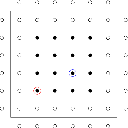
Figure 13: The path of Loop3(left) and Loop4(right). The blue circle indicates the link upward and the red circle indicates the link downward.
Refer to caption
Refer to caption
Figure 14: The path of Loop7(left) and Loop8(right).
Refer to caption
Refer to caption
Figure 15: The path of Loop9(left) and Loop10(right). .
Refer to caption
Refer to caption
Figure 16: The path of Loop13(left) and Loop14(right).
Refer to caption
Refer to caption
Figure 17: The path of Loop15(left) and Loop16(right).
Refer to caption
Figure 18: The path of Loop17.

When zz in DeGrand et al.DGHHN95 is replaced by e1∧e2e_{1}\wedge e_{2} and the difference scale of zz and tt is ignored we obtain for the Loop 3

L​3​[u1,u2]=t​3​[−14,u​1,u​2]×t​1​[−14,u1,u2+14]\displaystyle L3[u_{1},u_{2}]=t3[-\frac{1}{4},u1,u2]\times t1[-\frac{1}{4},u_{1},u_{2}+\frac{1}{4}]
×t​2​[−14,u1,u2+14]×t​3​[14,u1+14,u2+14]\displaystyle\times t2[-\frac{1}{4},u_{1},u_{2}+\frac{1}{4}]\times t3[\frac{1}{4},u_{1}+\frac{1}{4},u_{2}+\frac{1}{4}]
×t​2​[14,u1+14,u2]×t​1​[14,u1,u2].\displaystyle\times t2[\frac{1}{4},u_{1}+\frac{1}{4},u_{2}]\times t1[\frac{1}{4},u_{1},u_{2}].
Refer to caption
Figure 19: The absolute value of eigenvalues in Loop3 for a fixed u1u_{1} as a function of u2u_{2}. (Δ​ui=1\Delta u_{i}=1 (i=1,2)(i=1,2))
Refer to caption
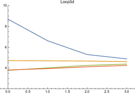
Figure 20: The absolute value of eigenvalues in Loop3d (Double step length Δ​t\Delta t.)

For the Loop 4

L​4​[u1,u2]=t​3​[−14,u​1,u​2]×t​2​[−14,u1,u2+14]\displaystyle L4[u_{1},u_{2}]=t3[-\frac{1}{4},u1,u2]\times t2[-\frac{1}{4},u_{1},u_{2}+\frac{1}{4}]
×t1[−14,u1+14,u2+14]×t314,u1+14,u2+14]\displaystyle\times t1[-\frac{1}{4},u_{1}+\frac{1}{4},u_{2}+\frac{1}{4}]\times t3\frac{1}{4},u_{1}+\frac{1}{4},u_{2}+\frac{1}{4}]
×t​2​[14,u1+14,u2]×t​1​[14,u1,u2].\displaystyle\times t2[\frac{1}{4},u_{1}+\frac{1}{4},u_{2}]\times t1[\frac{1}{4},u_{1},u_{2}].
Refer to caption
Figure 21: The absolute value of eigenvalues in Loop4 for a fixed u1u_{1} as a function of u2u_{2}. (Δ​ui=1\Delta u_{i}=1 (i=1,2)(i=1,2)).

For the Loop7

L​7​[u1,u2]=t​3​[−14,u1,u2]×t​1​[−12,u1+12,u2]\displaystyle L7[u_{1},u_{2}]=t3[-\frac{1}{4},u_{1},u_{2}]\times t1[-\frac{1}{2},u_{1}+\frac{1}{2},u_{2}]
×t​2​[−14,u1+14,u2+14]\displaystyle\times t2[-\frac{1}{4},u_{1}+\frac{1}{4},u_{2}+\frac{1}{4}]
×t​3​[12,u1+14,u2+14]×t​1​[14,u1+14,u2+14]\displaystyle\times t3[\frac{1}{2},u_{1}+\frac{1}{4},u_{2}+\frac{1}{4}]\times t1[\frac{1}{4},u_{1}+\frac{1}{4},u_{2}+\frac{1}{4}]
×t​2​[14,u1+14,u2]×t​1​[14,u1,u2].\displaystyle\times t2[\frac{1}{4},u_{1}+\frac{1}{4},u_{2}]\times t1[\frac{1}{4},u_{1},u_{2}].
Refer to caption
Figure 22: The absolute value of eigenvalues in Loop7 for a fixed u1u_{1} as a function of u2u_{2}. (Δ​ui=1\Delta u_{i}=1 (i=1,2)(i=1,2))

For the Loop8

L​8​[u1,u2]=t​2​[−14,u1,u2]×t​1​[−14,u1,u2+14]\displaystyle L8[u_{1},u_{2}]=t2[-\frac{1}{4},u_{1},u_{2}]\times t1[-\frac{1}{4},u_{1},u_{2}+\frac{1}{4}]
×t​3​[−14,u1+12,u2]×t​2​[−14,u1+12,u2+14]\displaystyle\times t3[-\frac{1}{4},u_{1}+\frac{1}{2},u_{2}]\times t2[-\frac{1}{4},u_{1}+\frac{1}{2},u_{2}+\frac{1}{4}]
×t​3​[14,u1+12,u2+14]×t​1​[14,u1+14,u2+14]\displaystyle\times t3[\frac{1}{4},u_{1}+\frac{1}{2},u_{2}+\frac{1}{4}]\times t1[\frac{1}{4},u_{1}+\frac{1}{4},u_{2}+\frac{1}{4}]
×t​2​[14,u1+14,u2]×t​1​[14,u1,u2].\displaystyle\times t2[\frac{1}{4},u_{1}+\frac{1}{4},u_{2}]\times t1[\frac{1}{4},u_{1},u_{2}].
Refer to caption
Figure 23: The absolute value of eigenvalues in Loop8 for a fixed u1u_{1} as a function of u2u_{2}. (Δ​ui=1\Delta u_{i}=1 (i=1,2)(i=1,2))

For the Loop9

L​9​[u1,u2]=t​3​[−14,u1,u2]×t​1​[−14,u1,u2]\displaystyle L9[u_{1},u_{2}]=t3[-\frac{1}{4},u_{1},u_{2}]\times t1[-\frac{1}{4},u_{1},u_{2}]
×t​2​[−14,u1,u2+14]×t​1​[−14,u1+14,u2+14]\displaystyle\times t2[-\frac{1}{4},u_{1},u_{2}+\frac{1}{4}]\times t1[-\frac{1}{4},u_{1}+\frac{1}{4},u_{2}+\frac{1}{4}]
×t​3​[14,u1+14,u2+14]×t​1​[14,u1+14,u2+14]\displaystyle\times t3[\frac{1}{4},u_{1}+\frac{1}{4},u_{2}+\frac{1}{4}]\times t1[\frac{1}{4},u_{1}+\frac{1}{4},u_{2}+\frac{1}{4}]
×t​2​[14,u1+14,u2]×t​1​[14,u1,u2].\displaystyle\times t2[\frac{1}{4},u_{1}+\frac{1}{4},u_{2}]\times t1[\frac{1}{4},u_{1},u_{2}].
Refer to caption
Figure 24: The absolute value of eigenvalues in Loop9 for a fixed u1u_{1} as a function of u2u_{2}. (Δ​ui=1\Delta u_{i}=1 (i=1,2)(i=1,2))

For the Loop10

L​10​[u1,u2]=t​2​[−14,u1,u2+14]×t​3​[−14,u1,u2+14]\displaystyle L10[u_{1},u_{2}]=t2[-\frac{1}{4},u_{1},u_{2}+\frac{1}{4}]\times t3[-\frac{1}{4},u_{1},u_{2}+\frac{1}{4}]
×t​1​[−12,u1+12,u2+14]×t​3​[14,u1+12,u2+14]\displaystyle\times t1[-\frac{1}{2},u_{1}+\frac{1}{2},u_{2}+\frac{1}{4}]\times t3[\frac{1}{4},u_{1}+\frac{1}{2},u_{2}+\frac{1}{4}]
×t​1​[14,u1+14,u2+14]×t​2​[14,u1+14,u2]×t​1​[14,u1,u2].\displaystyle\times t1[\frac{1}{4},u_{1}+\frac{1}{4},u_{2}+\frac{1}{4}]\times t2[\frac{1}{4},u_{1}+\frac{1}{4},u_{2}]\times t1[\frac{1}{4},u_{1},u_{2}].
Refer to caption
Figure 25: The absolute value of eigenvalues in Loop10 for a fixed u1u_{1} as a function of u2u_{2}. (Δ​ui=1\Delta u_{i}=1 (i=1,2)(i=1,2))

For the Loop13

L​13​[u1,u2]=t​3​[−14,u1,u2+14]×t​1​[−14,u1+14,u2+14]\displaystyle L13[u_{1},u_{2}]=t3[-\frac{1}{4},u_{1},u_{2}+\frac{1}{4}]\times t1[-\frac{1}{4},u_{1}+\frac{1}{4},u_{2}+\frac{1}{4}]
×t3[−14,u1+14,u2+14]×t2[−14,u1+14,u2+1/2]×\displaystyle\times t3[-\frac{1}{4},u_{1}+\frac{1}{4},u_{2}+\frac{1}{4}]\times t2[-\frac{1}{4},u_{1}+\frac{1}{4},u_{2}+1/2]\times
×t​3​[14,u1+14,u2+12]×t​2​[12,u1+14,u2]×t​1​[14,u1,u2].\displaystyle\times t3[\frac{1}{4},u_{1}+\frac{1}{4},u_{2}+\frac{1}{2}]\times t2[\frac{1}{2},u_{1}+\frac{1}{4},u_{2}]\times t1[\frac{1}{4},u_{1},u_{2}].
Refer to caption
Figure 26: The absolute value of eigenvalues in Loop13 for a fixed u1u_{1} as a function of u2u_{2}. (Δ​ui=1\Delta u_{i}=1 (i=1,2)(i=1,2))

For the Loop14

L​14​[u1,u2]=t​3​[−14,u1,u2]×t​1​[−14,u1+14,u2]\displaystyle L14[u_{1},u_{2}]=t3[-\frac{1}{4},u_{1},u_{2}]\times t1[-\frac{1}{4},u_{1}+\frac{1}{4},u_{2}]
×t​2​[−12,u1+14,u2+12]×t​3​[14,u1+14,u​2+12]\displaystyle\times t2[-\frac{1}{2},u_{1}+\frac{1}{4},u_{2}+\frac{1}{2}]\times t3[\frac{1}{4},u_{1}+\frac{1}{4},u2+\frac{1}{2}]
×t​2​[12,u1+14,u2]×t​1​[14,u1,u2].\displaystyle\times t2[\frac{1}{2},u_{1}+\frac{1}{4},u_{2}]\times t1[\frac{1}{4},u_{1},u_{2}].
Refer to caption
Figure 27: The absolute value of eigenvalues in Loop14 for a fixed u1u_{1} as a function of u2u_{2}. (Δ​ui=1\Delta u_{i}=1 (i=1,2)(i=1,2))

For the Loop15

L​15​[u1,u2]=t​2​[−14,u1,u2+14]×t​3​[−14,u1,u2+14]\displaystyle L15[u_{1},u_{2}]=t2[-\frac{1}{4},u_{1},u_{2}+\frac{1}{4}]\times t3[-\frac{1}{4},u_{1},u_{2}+\frac{1}{4}]
×t​1​[−14,u1+14,u2+14]×t​2​[−14,u1+14,u2+12]\displaystyle\times t1[-\frac{1}{4},u_{1}+\frac{1}{4},u_{2}+\frac{1}{4}]\times t2[-\frac{1}{4},u_{1}+\frac{1}{4},u_{2}+\frac{1}{2}]
×t​3​[14,u1+14,u2+12]×t​2​[12,u1+14,u2]×t​1​[14,u1,u2].\displaystyle\times t3[\frac{1}{4},u_{1}+\frac{1}{4},u_{2}+\frac{1}{2}]\times t2[\frac{1}{2},u_{1}+\frac{1}{4},u_{2}]\times t1[\frac{1}{4},u_{1},u_{2}].
Refer to caption
Figure 28: The absolute value of eigenvalues in Loop15 for a fixed u1u_{1} as a function of u2u_{2}. (Δ​ui=1\Delta u_{i}=1 (i=1,2)(i=1,2))

For the Loop16

L​16​[u1,u2]=t​3​[−14,u1,u2]×t​2​[−14,u1,u2+14]\displaystyle L16[u_{1},u_{2}]=t3[-\frac{1}{4},u_{1},u_{2}]\times t2[-\frac{1}{4},u_{1},u_{2}+\frac{1}{4}]
×t​1​[−12,u1+12,u2+14]×t​3​[14,u1+12,u2+14]\displaystyle\times t1[-\frac{1}{2},u_{1}+\frac{1}{2},u_{2}+\frac{1}{4}]\times t3[\frac{1}{4},u_{1}+\frac{1}{2},u_{2}+\frac{1}{4}]
×t​1​[14,u1+14,u2+14]×t​2​[14,u1+14,u2]×t​1​[14,u1,u2].\displaystyle\times t1[\frac{1}{4},u_{1}+\frac{1}{4},u_{2}+\frac{1}{4}]\times t2[\frac{1}{4},u_{1}+\frac{1}{4},u_{2}]\times t1[\frac{1}{4},u_{1},u_{2}].
Refer to caption
Figure 29: The absolute value of eigenvalues in Loop16 for a fixed u1u_{1} as a function of u2u_{2}. (Δ​ui=1\Delta u_{i}=1 (i=1,2)(i=1,2))

For the Loop17

L​17​[u1,u2]=t​3​[−14,u1,u2]×t​2​[−12,u1,u2+12]\displaystyle L17[u_{1},u_{2}]=t3[-\frac{1}{4},u_{1},u_{2}]\times t2[-\frac{1}{2},u_{1},u_{2}+\frac{1}{2}]
×t​3​[14,u1,u2+12]×t​1​[−14,u1+14,u2+12]\displaystyle\times t3[\frac{1}{4},u_{1},u_{2}+\frac{1}{2}]\times t1[-\frac{1}{4},u_{1}+\frac{1}{4},u_{2}+\frac{1}{2}]
×t​2​[12,u1+14,u2]×t​1​[14,u1,u2].\displaystyle\times t2[\frac{1}{2},u_{1}+\frac{1}{4},u_{2}]\times t1[\frac{1}{4},u_{1},u_{2}].
Refer to caption
Figure 30: The absolute value of eigenvalues in Loop17 for a fixed u1u_{1} as a function of u2u_{2}. (Δ​ui=1\Delta u_{i}=1 (i=1,2)(i=1,2))

The absolute value of the eigenvalues of d​𝐒​[0,i]d{\bf S}[0,i] (Blue),d​𝐒​[1,i]d{\bf S}[1,i] (Orange), d​𝐒​[2,i]d{\bf S}[2,i] (Green), d​𝐒​[3,i]d{\bf S}[3,i] (Red) for i=0,1,2,3i=0,1,2,3 are plotted in Fig,19 to Fig.30.

The scale of e3=e1∧e2e_{3}=e_{1}\wedge e_{2} cannot be fixed a priori. I took Δ​e1=Δ​e2=1/4\Delta e_{1}=\Delta e_{2}=1/4, Δ​e3=1/2\Delta e_{3}=1/2.

I compared the eigenvalues of Loop3 and that of Loop3d, in which Δ​e1=Δ​e2=Δ​e3=1/2\Delta e_{1}=\Delta e_{2}=\Delta e_{3}=1/2.

The loop L​3​[0,0]L3[0,0] has the eigenvalue

χ⁡(L​3​[0,0])=−5.33311±6.86919​−1\chi(L3[0,0])=-5.33311\pm 6.86919\sqrt{-1}

and eigen-quaternion

𝐒⁡(L​3​[0,0])\displaystyle{\bf S}(L3[0,0]) =\displaystyle= 0.594603​−1​e1+0.306216​−1​e0\displaystyle 0.594603\sqrt{-1}e_{1}+0.306216\sqrt{-1}e_{0}
−0.743424​−1​e1∧e2.\displaystyle-0.743424\sqrt{-1}e_{1}\wedge e_{2}.

The loop L​3​d​[0,0]L3d[0,0] has the eigenvalue

χ⁡(L​3​d​[0,0])=−6.37495±7.44031​−1\chi(L3d[0,0])=-6.37495\pm 7.44031\sqrt{-1}

and the eigen-quaternion

𝐒⁡(L​3​d​[0,0])\displaystyle{\bf S}(L3d[0,0]) =\displaystyle= 0.180682​−1​e1+0.263462​−1​e0\displaystyle 0.180682\sqrt{-1}e_{1}+0.263462\sqrt{-1}e_{0}
−0.947598​−1​e1∧e2.\displaystyle-0.947598\sqrt{-1}e_{1}\wedge e_{2}.

The eigenvalues χ⁡(L​3​[i,j])\chi(L3[i,j]) (0≤i,j≤1)(0\leq i,j\leq 1) give the plaquette part of the Wilson loop.

Along the path L​3​[0,0]L3[0,0],

d​𝐒​(L​3​[0,0])\displaystyle d{\bf S}(L3[0,0]) =\displaystyle= d​S1​[0,0]+d​S2​[14,0]+d​S3​[14,14]\displaystyle dS_{1}[0,0]+dS_{2}[\frac{1}{4},0]+dS_{3}[\frac{1}{4},\frac{1}{4}] (18)
−d​S2​[14,14]−d​S1​[14,0]−d​S3​[14,0]\displaystyle-dS_{2}[\frac{1}{4},\frac{1}{4}]-dS_{1}[\frac{1}{4},0]-dS_{3}[\frac{1}{4},0]

has a non-zero quaternion element in the right-upper corner of the 4×44\times 4 matrix, and other elements are zero.

The sum over d​𝐒​(L)d{\bf S}(L) corresponds to the loop part, and the sum over χ⁡(L)\chi(L) corresponds to the interpolating surface part of the Wilson actionWilson74 in the lattice gauge theory.

It can be checked by comparing the χ⁡(L​1​[0,0])×4∼χ⁡(L​28​[0,0])=\chi(L1[0,0])\times 4\sim\chi(L28[0,0])=, and d​𝐒​(L​1​[0,0])×2=d​𝐒​(L​28​[0,0]).d{\bf S}(L1[0,0])\times 2=d{\bf S}(L28[0,0]).

III Recursive renormalization group analysis of (2+1)​D(2+1)D lattices

We try to derive the effective action of the Weyl spinors by making the lattice spacing reduced by multilpying a factor 1/21/2 at each step.

Migdal Migdal75a; Migdal75b derived the scaling relation of the partition function in DD dimensional system

Z2​L[𝐒[Γ=∫∏(d𝐒i​n​t∏i=14ZL[𝐒γ​i]\displaystyle Z_{2L}[{\bf S}[_{\Gamma}=\int\prod(d{\bf S}_{int}\prod_{i=1}^{4}Z_{L}[{\bf S}_{\gamma i}]
(d𝐒)=dn𝐒δ(1−𝐒2)Γ(n/2)π−n/2\displaystyle(d{\bf S})=d^{n}{\bf S}\delta(1-{\bf S}^{2})\Gamma(n/2)\pi^{-n/2}

where [𝐒γ​i][{\bf S}_{\gamma i}] is the set of of spins on the boundaryof the 2​L2L-square, [𝐒γ​i][{\bf S}_{\gamma i}] is the sets of spins on the boundary of LL-squares and [𝐒i​n​t][{\bf S}_{int}] are the spins on the internal boundaries of the LL-squares.

The Migdal-Kadanoff (MK) renormalization technique in 𝐙2{\bf Z}^{2} model Creutz80; Migdal75a; Migdal75b; Kadanoff77 is to define the partition function Z=T​r​(T​(β0,β1)2)=T​r​(T′​(β0′,β1′))Z=Tr(T(\beta_{0},\beta_{1})^{2})=Tr(T^{\prime}(\beta_{0}^{\prime},\beta_{1}^{\prime})) that satisfy renormalization group equation.

The parameters β0,β1\beta_{0},\beta_{1} are obtained by solving

T2=[eβ0​(eβ1e−β1e−β1eβ1)]2=eβ0′​(eβ1′e−β1′e−β1′eβ1′)\displaystyle T^{2}=[e^{\beta_{0}}\left(\begin{array}[]{cc}e^{\beta_{1}}&e^{-\beta_{1}}\\ e^{-\beta_{1}}&e^{\beta_{1}}\end{array}\right)]^{2}=e^{\beta_{0}^{\prime}}\left(\begin{array}[]{cc}e^{\beta_{1}^{\prime}}&e^{-\beta_{1}^{\prime}}\\ e^{-\beta_{1}^{\prime}}&e^{\beta_{1}^{\prime}}\end{array}\right)
=T′​(β0′,β1′).\displaystyle=T^{\prime}(\beta_{0}^{\prime},\beta_{1}^{\prime}).

A solution is

β0\displaystyle\beta_{0} ′={}^{\prime}= 12​(4​β0+log⁡(4​cosh⁡(2​β1))CLOSE,\displaystyle\frac{1}{2}(4\beta_{0}+\log(4\cosh(2\beta_{1})),
β1′\displaystyle\beta_{1}^{\prime} =\displaystyle= 12​log⁡(cosh⁡(2​β1)).\displaystyle\frac{1}{2}\log(\cosh(2\beta_{1})).

In 2​D2D MK recursions, β1=(log⁡(1+2))/2\beta_{1}=({\log(1+{\sqrt{2}}))}/{2} is a self dual point.

The renormalization theory of quantized systems wasdiscussed by Gallavotti Gallavotti85. A string Lagrangian and wave functions e−1​(k​x−ℰ​(k)​t)e^{\sqrt{-1}(kx-{\mathcal{E}}(k)t)}, where

ℰ⁡(k)=±(ω2+c2​k2)1/2,\displaystyle{\mathcal{E}}(k)=\pm(\omega^{2}+c^{2}k^{2})^{1/2},
p=ℏ​k,E=ℏ​ℰ.\displaystyle p=\hbar k,\quad E=\hbar{\mathcal{E}}.

The relation between the momentum pp and the velocity vv is

v=d​ℰd​k=c2​k(ω2+c2​k2)1/2\displaystyle v=\frac{d{\mathcal{E}}}{dk}=\frac{c^{2}k}{(\omega^{2}+c^{2}k^{2})^{1/2}}
p=v​ω​ℏ/c2(1−v2/c2)1/2.\displaystyle p=v\frac{\omega\hbar/c^{2}}{(1-v^{2}/c^{2})^{1/2}}.

For lattice simulation of propagation of ultrasonic waves in 2​D2D media, we adopt Luescher’s domain decomposition methodLuescher98a; Luescher98b; Luescher03.

The choice of quaternion projective space on 2​D2D planes is expected to reduce number of training parameters. Numerical calculation of the Generalized Conjugate Residual (GCR) method proposed by Luescher is to estimate the acceptance vs reject probability P⁡(C,C′)P(C,C^{\prime}).

The propagation in e1∧e2e_{1}\wedge e_{2} should contain information on the effective mass of the Weyl spinor.

IV Application of Luescher’s Action to the Symplectic group C​ℓ1,3+C\ell_{1,3}^{+}

In general, physical dynamics are represented by unitary group U⁡(n)U(n), which has bases of 𝐂{\bf C}, orthogonal group O⁡(n)O(n), which has bases of 𝐑{\bf R}, and the symplectic group S​p​(n)Sp(n), which has bases of 𝐇{\bf H}Souriau70; Hestenes86; Porteous95; Lounesto01.

In the Clifford algebra, transformation X→X′X\to X^{\prime} by a spin transformation (acbd)\left(\begin{array}[]{cc}a&c\\ b&d\end{array}\right) is represented byPorteous95

(acbd)​(xx​x−Ix−)​(d−c−b−a−)=λ​(x′x′​x′⁣−Ix′⁣−),\left(\begin{array}[]{cc}a&c\\ b&d\end{array}\right)\left(\begin{array}[]{cc}x&xx^{-}\\ I&x^{-}\end{array}\right)\left(\begin{array}[]{cc}d^{-}&c^{-}\\ b^{-}&a^{-}\end{array}\right)=\lambda\left(\begin{array}[]{cc}x^{\prime}&x^{\prime}x^{\prime-}\\ I&x^{\prime-}\end{array}\right),

eigenvalues χ\chi can be obtained from the 2×22\times 2 matrix of the left-down corner of the 4×44\times 4 matrix.

We calculate L⁡[u1,u2]L[u_{1},u_{2}] in 4×44\times 4 matrices and pickup left-down corner 2×22\times 2 complex matrices and calculates their eigen quaternions.

Since the system is time-reversal symmetric, the two eigenvalues are conjugate with each other. It is a characteristic for TR symmetric systems.

The eigenvalues of the plaquett matrices corresponding to the Wilson loops on a planehave dependences on [u1,u2][u_{1},u_{2}] when it is close to [0,0][0,0].

Using the parametrization of 𝐒⁡[u1,u2]{\bf S}[u_{1},u_{2}], we define

∂1𝐒=lima→0(𝒯(1,0)​𝐒​𝒯(1,0)−1−𝐒)/a.\partial_{1}{\bf S}=\lim_{a\to 0}({\mathcal{T}}_{(1,0)}{\bf S}{{\mathcal{T}}_{(1,0)}}^{-1}-{\bf S})/a.

Similarly, we define ∂2𝐒\partial_{2}{\bf S}.

The real part and the imaginary part of ∂i𝐒⁡(u1,u2)\partial_{i}{\bf S}(u_{1},u_{2}) (i=1,2)(i=1,2) in the region −1≤u1≤1-1\leq u_{1}\leq 1 and −1≤u2≤1-1\leq u_{2}\leq 1 are plotted in Fig. 35 and Fig. 35.

Refer to caption
Refer to caption
Figure 31: The real part of ∂1𝐒⁡[u1,u2]\partial_{1}{\bf S}[u_{1},u_{2}] (left) and the imaginary part of ∂1𝐒⁡[u1,u2]\partial_{1}{\bf S}[u_{1},u_{2}] (right).
Refer to caption
Refer to caption
Figure 32: The real part of ∂2𝐒⁡[u1,u2]\partial_{2}{\bf S}[u_{1},u_{2}] (left) and the imaginary part of OPEN∂2𝐒⁡[u1,u2])\partial_{2}{\bf S}[u_{1},u_{2}]).
Refer to caption
Refer to caption
Figure 33: The real part of ∂3𝐒⁡[u1,u2]\partial_{3}{\bf S}[u_{1},u_{2}] (left) and the imaginary part of ∂3𝐒⁡[u1,u2]\partial_{3}{\bf S}[u_{1},u_{2}] (right).
Refer to caption
Figure 34: ∂i𝐒⋅∂i𝐒~​[u1,u2]\partial_{i}{\bf S}\cdot\partial_{i}{\tilde{\bf S}}[u_{1},u_{2}] (i=1,2)(i=1,2)
Refer to caption
Figure 35: ∂3𝐒⋅∂3𝐒~​[u1,u2]\partial_{3}{\bf S}\cdot\partial_{3}{\tilde{\bf S}}[u_{1},u_{2}].

The wedge product e1∧e2=e3e_{1}\wedge e_{2}=e_{3} yields

∂3𝐒⁡[u1,u2]=lima→0(𝒯(1,1)​𝐒​𝒯(1,1)−1−𝐒)/a.\partial_{3}{\bf S}[u_{1},u_{2}]=\lim_{a\to 0}({\mathcal{T}}_{(1,1)}{\bf S}{{\mathcal{T}}_{(1,1)}}^{-1}-{\bf S})/a.

Its real and imaginary part are plotted in Fig.35.

The action in Clifford algebra is a discrete sum
∑∂μ𝐒⁡(u1,u2)⋅∂μ𝐒~​(u1,u2)\sum\partial_{\mu}{\bf S}(u_{1},u_{2})\cdot\partial_{\mu}{\tilde{\bf S}}(u_{1},u_{2}), for −1≤u1,u2≤1-1\leq u_{1},u_{2}\leq 1 with an appropriate measure.

∂i𝐒⋅∂i𝐒~​[u1,u2]\partial_{i}{\bf S}\cdot\partial_{i}{\tilde{\bf S}}[u_{1},u_{2}] for i=1,2i=1,2 is

∂i𝐒⋅∂i𝐒~​[u1​u2]=\displaystyle\partial_{i}{\bf S}\cdot\partial_{i}{\tilde{\bf S}}[u_{1}u_{2}]=
4​u13+u14+4​u1​(−1+u22)+2​u12​(1+u22)+(1+u22)2(1+|u|2)2,\displaystyle\frac{4{u_{1}}^{3}+{u_{1}}^{4}+4u_{1}(-1+{u_{2}}^{2})+2{u_{1}}^{2}(1+{u_{2}}^{2})+(1+{u_{2}}^{2})^{2}}{(1+|u|^{2})^{2}},

which is shown in Fig.35.

For i=3i=3

∂3𝐒⋅∂3𝐒~​[u1​u2]=\displaystyle\partial_{3}{\bf S}\cdot\partial_{3}{\tilde{\bf S}}[u_{1}u_{2}]=
−4​u13+u14−4​u1​(−1+u22)+2​u12​(1+u22)+(1+u22)2(1+|u|2)2.\displaystyle\frac{-4{u_{1}}^{3}+{u_{1}}^{4}-4u_{1}(-1+{u_{2}}^{2})+2{u_{1}}^{2}(1+{u_{2}}^{2})+(1+{u_{2}}^{2})^{2}}{(1+|u|^{2})^{2}}.

is shown in Fig.35.

Refer to caption
Figure 36: β0′−2​β0\beta_{0}^{\prime}-2\beta_{0} as a function of β1\beta_{1} of Clifford algebra. At β1=0\beta_{1}=0, it has the minimum log⁡2\log 2. β0′−2​β0\beta_{0}^{\prime}-2\beta_{0} in MK method is indicated by red line.
Refer to caption
Figure 37: β1′/−1\beta_{1}^{\prime}/\sqrt{-1} as a function of β1\beta_{1} in Clifford algebra.
At β1=±log⁡(1+2)=±0.881374\beta_{1}=\pm\log(1+{\sqrt{2}})=\pm 0.881374 it has the maximum 0.463648. β1′\beta_{1}^{\prime} in MK method is indicated by red line

In the Clifford algebra, the MK renormalization is modified to the equation

2​T2=T′​(β0′,β1′).2T^{2}=T^{\prime}(\beta_{0}^{\prime},\beta_{1}^{\prime}).

The difference of a factor 2 in the left hand side of the equation from that of MK is due to the choice of normalization ∑s1=2\sum_{s}1=2 Creutz80.

Since for 𝐚,𝐛∈𝐇{\bf a},{\bf b}\in{\bf H}, 𝐚𝐛=−𝐚⋅𝐛+𝐚∧𝐛{\bf ab}=-{\bf a}\cdot{\bf b}+{\bf a}\wedge{\bf b}, there appears a factor of −1\sqrt{-1} difference in β1′\beta_{1}^{\prime}.

T\displaystyle T =\displaystyle= eβ0​(cosh⁡(β1)​e0+sinh⁡(β1)​e1∧e2)\displaystyle e^{\beta_{0}}(\cosh(\beta_{1})e_{0}+\sinh(\beta_{1})e_{1}\wedge e_{2})
=\displaystyle= eβ0​(cosh⁡(β1)−1​sinh⁡(β1)−1​sinh⁡(β1)cosh⁡(β1)).\displaystyle e^{\beta_{0}}\left(\begin{array}[]{cc}\cosh(\beta_{1})&\sqrt{-1}\sinh(\beta_{1})\\ \sqrt{-1}\sinh(\beta_{1})&\cosh(\beta_{1})\end{array}\right).
β0′\displaystyle\beta_{0}^{\prime} =\displaystyle= log[2e2​β0(cosh⁡(β1)4cosh⁡(β1)4+sinh⁡(β1)2\displaystyle\log[2e^{2\beta_{0}}(\frac{\cosh(\beta_{1})^{4}}{\cosh(\beta_{1})^{4}+\sinh(\beta_{1})^{2}}
+sinh⁡(β1)2cosh⁡(β1)4+sinh⁡(β1)2)],\displaystyle+\frac{\sinh(\beta_{1})^{2}}{\cosh(\beta_{1})^{4}+\sinh(\beta_{1})^{2}})],
β1′\displaystyle\beta_{1}^{\prime} =\displaystyle= cosh−1⁡(cosh⁡(β1)2cosh⁡(β1)4+sinh⁡(β1)2).\displaystyle\cosh^{-1}(\frac{\cosh(\beta_{1})^{2}}{\cosh(\beta_{1})^{4}+\sinh(\beta_{1})^{2}}).

β0\beta_{0} and β1/−1\beta_{1}/\sqrt{-1} in the Clifford algebra and corresponding β0\beta_{0} and β1\beta_{1} in the Unitary algebra are shown in Fig,36 and Fig.37.

V Renormalization group and the scaling problem

In order to study propagation of a phonon or a poson in fermions filled up to Fermi momentum pFp_{F}, renormalization group approach of Benfatto and GallavottiBG95 is useful.

GallavottiGallavotti85 studied a specific Hamiltonian

Hq​u​a​n​t​u​m\displaystyle H_{quantum} =\displaystyle= −ℏ22​μ​aD2∑n¯​a∈λ0∂2∂φn¯​a\displaystyle-\frac{\hbar^{2}}{{2\mu a^{D}}^{2}}\sum_{{\bar{n}a}\in\lambda_{0}}\frac{\partial^{2}}{\partial\varphi_{\bar{n}a}} (27)
+μaD2∑n¯​a∈Λ0[c2∑j=1D(φn¯​a+ϵ¯j​a−φn¯​a)2/a2\displaystyle+\mu\frac{a^{D}}{2}\sum_{\bar{n}a\in\Lambda_{0}}[c^{2}\sum_{j=1}^{D}(\varphi_{\bar{n}a+\bar{\epsilon}_{j}a}-\varphi_{\bar{n}a})^{2}/a^{2}
+(m0​c2/ℏ)2​φn¯​s2+I⁡(φn¯​a)\displaystyle+(m_{0}c^{2}/\hbar)^{2}\varphi_{\bar{n}s}^{2}+I(\varphi_{\bar{n}a})

where I⁡(φn¯​a)I(\varphi_{\bar{n}a}) is a function of φn¯​a\varphi_{\bar{n}a} bounded below.

On the L2L_{2} space with the Gaussian measure

d′′​φ′′=∏x¯∈λ0d​φ​(x¯),{}^{\prime\prime}d\varphi^{\prime\prime}=\prod_{\bar{x}\in\lambda_{0}}d\varphi(\bar{x}),

is

Tt=exp[−(Hq​u​a​n​t​u​m−E)t/ℏ],t≥0T_{t}=exp[-(H_{quantum}-E)t/\hbar],\quad t\geq 0

one defines e⁡(φ¯)=e(\bar{\varphi})= ground state wave function for HquantumH_{\rm quantum} and put a suffix 00 for values for t=0t=0, eg H0=Hquantum|t=0H_{0}=H_{\rm quantum}|_{t=0}.

Tt0​(φ¯,φ¯′)=kernel​of​Tt​onL2​[∏n¯​ad​φn¯​a]T_{t}^{0}(\bar{\varphi},\bar{\varphi}^{\prime})={\rm kernel\,of\,}T_{t}{\rm on}\quad L_{2}[\prod_{\bar{n}a}d\varphi_{\bar{n}a}].

Multiscale decomposition of the system is performed as

Cξ,η=∑n¯∈ZDC¯x¯+n¯​L,t​(y¯,t′),C_{\xi,\eta}=\sum_{\bar{n}\in Z^{D}}\bar{C}_{\bar{x}+\bar{n}L,t}(\bar{y},t^{\prime}),

where ξ=(n¯​a,t)∈Λ0×S1\xi=(\bar{n}a,t)\in\Lambda_{0}\times S^{1} and η=(m¯​a,t′)\eta=(\bar{m}a,t^{\prime}). We replace 𝐑{\bf R} ofGallavotti85 to S1S^{1}SF20 for the lattice simulation.

The measure P⁡(d​φ)P(d\varphi) becomes

P⁡(d​φ)\displaystyle P(d\varphi) =\displaystyle= Z−1[exp{−μ​b​aD2​ℏ∑n¯​a∈λ0∑m[{(φn¯​a,m​b−φn¯​a,m​b+b)2/b2\displaystyle Z^{-1}[exp\{-\frac{\mu ba^{D}}{2\hbar}\sum_{\bar{n}a\in\lambda_{0}}\sum_{m}[\{(\varphi_{\bar{n}a,mb}-\varphi_{\bar{n}a,mb+b})^{2}/b^{2}
+c2∑j=1D(φn¯​a,m​b−φn¯​a+e¯j​a,m​b)2/a2}\displaystyle+c^{2}\sum_{j=1}^{D}(\varphi_{\bar{n}a,mb}-\varphi_{\bar{n}a+\bar{e}_{j}a,mb})^{2}/a^{2}\}
+(m0c2/ℏ)2φn¯​a,m​b+I(φn¯​a,m​b)}]∏n¯,mdφn¯,m​b\displaystyle+(m_{0}c^{2}/\hbar)^{2}\varphi_{\bar{n}a,mb}+I(\varphi_{\bar{n}a,mb})\}]\prod_{\bar{n},m}d\varphi_{\bar{n},mb}

One defines the measure

P(≤N)​(d​φ)\displaystyle P^{(\leq N)}(d\varphi) =\displaystyle= ZN,a−1[exp{−μ​ad2​c​ℏ∑ξI(φξ(≤N)}]\displaystyle Z_{N,a}^{-1}[exp\{-\frac{\mu a^{d}}{2c\hbar}\sum_{\xi}I(\varphi_{\xi}^{(\leq N)}\}] (28)
×∏j=0NP⁡(d​φ(j)),\displaystyle\times\prod_{j=0}^{N}P(d\varphi^{(j)}),

The interaction I⁡(φ)I(\varphi) is assumed to have the form

V⁡(φ(≤N),λ¯,N)\displaystyle V(\varphi^{(\leq N)},\bar{\lambda},N) =\displaystyle= ∑α=1tλ(α)​∫ΛvNα​(φξ(≤N),∂φξ(≤N))​𝑑ξ\displaystyle\sum_{\alpha=1}^{t}\lambda^{(\alpha)}\int_{\Lambda}v_{N}^{\alpha}(\varphi_{\xi}^{(\leq N)},\partial\varphi_{\xi}^{(\leq N)})d\xi (29)

in the continuum.

For all N′≤NN^{\prime}\leq N,

∫ΛvN′(α)​(φξ(≤N′),∂φξ(≤N′)​𝑑ξCLOSE\displaystyle\int_{\Lambda}v_{N^{\prime}}^{(\alpha)}(\varphi_{\xi}^{(\leq N^{\prime})},\partial\varphi_{\xi}^{(\leq N^{\prime})}d\xi
=∫P(dφ(N′+1))⋯P(dφ(N))∫ΛvN(α)(φx(≤N),∂φξ(≤N))dξ.\displaystyle=\int P(d\varphi^{(N^{\prime}+1)})\cdots P(d\varphi^{(N)})\int_{\Lambda}v_{N}^{(\alpha)}(\varphi_{x}^{(\leq N)},\partial\varphi_{\xi}^{(\leq N)})d\xi.

The effective interaction of the fields φ(0),⋯,φ(k)\varphi^{(0)},\cdots,\varphi^{(k)} on their own length scale γ−k​m−1\gamma^{-k}m^{-1} is

eV(k),φ(≤k)\displaystyle e^{V^{(k)},\varphi^{(\leq k)}} =\displaystyle= ∫exp[V(φ(≤N)]\displaystyle\int exp[V(\varphi^{(\leq N)}] (31)
×P(dφ(N))⋯P(dφ(k+1)).\displaystyle\times P(d\varphi^{(N)})\cdots P(d\varphi^{(k+1)}).

One defines the expectation value with respect to a probability measure as ℰ⁡(){\mathcal{E}}(), the expectation value with respect to the Gaussian measure P⁡(d​φ(k))P(d\varphi^{(k)}) as ℰk​(){\mathcal{E}}_{k}(), and pp random variables x1,⋯,xpx_{1},\cdots,x_{p} of orders n1,⋯,npn_{1},\cdots,n_{p}.

The truncated expectations of x1,⋯,xpx_{1},\cdots,x_{p} of orders n1,⋯,npn_{1},\cdots,n_{p} are

ℰT​(x1,⋯,xp,n1,⋯,np)\displaystyle{\mathcal{E}}^{T}(x_{1},\cdots,x_{p};n_{1},\cdots,n_{p})
=∂n1+⋯+np∂λ1n1⋯∂λpnp​log⁡ℰ⁡(eλ1​x1+⋯+λp​xp)|λ1=⋯=λp=0\displaystyle=\frac{\partial^{n_{1}+\cdots+n_{p}}}{\partial\lambda_{1}^{n_{1}}\cdots\partial\lambda_{p}^{n_{p}}}\log{\mathcal{E}}(e^{\lambda_{1}x_{1}+\cdots+\lambda_{p}x_{p}})|_{\lambda_{1}=\cdots=\lambda_{p}=0}

For ω,⋯,ωp∈𝐑\omega_{,}\cdots,\omega_{p}\in{\bf R}

ℰT​(ω1​x1+⋯+ωp​xp,n)\displaystyle{\mathcal{E}}^{T}(\omega_{1}x_{1}+\cdots+\omega_{p}x_{p};n)
=∑n1,⋯,np|n1+⋯+np=nn!ω1n1⋯ωpnpn1!⋯np!\displaystyle=\sum_{n_{1},\cdots,n_{p}|n_{1}+\cdots+n_{p}=n}\frac{n!\omega_{1}^{n_{1}}\cdots\omega_{p}^{n_{p}}}{n_{1}!\cdots n_{p}!}
×ℰT​(x1,⋯,xp,n1,⋯,np).\displaystyle\quad\quad\times{\mathcal{E}}^{T}(x_{1},\cdots,x_{p};n_{1},\cdots,n_{p}).

When one ignores the convergence conditions

∫P⁡(d​φ(N))​eV\displaystyle\int P(d\varphi^{(N)})e^{V} ≡\displaystyle\equiv e​x​p​[∑n=1∞ℰNT​(V,n)n]\displaystyle exp[\sum_{n=1}^{\infty}\frac{{\mathcal{E}}_{N}^{T}(V;n)}{n\!}]
=\displaystyle= e​x​p​[V(N−1)],\displaystyle exp[V^{(N-1)}],

where ℰT​(V,n)=ℰT​(x1,⋯,xp,n1,⋯,np){\mathcal{E}}^{T}(V;n)={\mathcal{E}}^{T}(x_{1},\cdots,x_{p};n_{1},\cdots,n_{p}).

In the case of dd dimensional Fermi liquid, the propoagatorBG95

g¯​(x)=1(2​π)d+1​∫e−(k02+ℰ(𝐤)2)/p02e−−1​k​x−−1​k0+ℰ⁡(𝐤)​dd+1​k\bar{g}(x)=\frac{1}{(2\pi)^{d+1}}\int\frac{e^{-(k_{0}^{2}+{\mathcal{E}}({\bf k})^{2})/{p_{0}}^{2}}e^{-\sqrt{-1}kx}}{-\sqrt{-1}k_{0}+{\mathcal{E}}({\bf k})}d^{d+1}k

where ℰ⁡(𝐤)=(𝐤2−pF2)/2​m{\mathcal{E}}({\bf k})=({\bf k}^{2}-{p_{F}}^{2})/2m.

In the case of spatial 1DD

g¯(x−y)=∑ω=±1∫e−−1​k​(x−y)−−1​k0+ω⋅ke−−1pFω⋅(x−y)d2k\bar{g}(x-y)=\sum_{\omega=\pm 1}\int\frac{e^{-\sqrt{-1}k(x-y)}}{-\sqrt{-1}k_{0}+\omega\cdot k}e^{-\sqrt{-1}p_{F}\omega\cdot(x-y)}d^{2}k

One performs multiscale decomposition of the scalar field

ψx=∑h=−∞0ψx(h)\psi_{x}=\sum_{h=-\infty}^{0}\psi_{x}^{(h)}

where ψx(h)\psi_{x}^{(h)} are Gaussian fields with propagators

δh​h′​C~​(2h​p0​(x−y))​2(d−2+γ)​h,\delta_{hh^{\prime}}{\tilde{C}}(2^{h}p_{0}(x-y))2^{(d-2+\gamma)h},

and ψx(h)\psi_{x}^{(h)} is the same as that of ψx(0)\psi_{x}^{(0)} suitably rescaled

ψx(h)=2(d−2+γ)​h/2​ψ2h​x(0).\psi_{x}^{(h)}=2^{(d-2+\gamma)h/2}\psi_{2^{h}x}^{(0)}.

Here the potential between fermions are assumed to be long range J⁡(x)∝|x|−αJ(x)\propto|x|^{-\alpha} and γ=d+2−α\gamma=d+2-\alpha.

The propagator for the Bose gas is

g(t)​(x)=1(2​π)d+1​∫d​k​e−1​k​x​t⁡(k)−−1​k0+𝐤22​mg^{(t)}(x)=\frac{1}{(2\pi)^{d+1}}\int dke^{\sqrt{-1}kx}\frac{t(k)}{-\sqrt{-1}k_{0}+\frac{{\bf k}^{2}}{2m}}

where t⁡(k)t(k) is a positive cutoff function.

Consider the fields

χx±=12​ρ​(ψx+±ψx−)=1(2​π)d−1​∫d​k​e±−1​k​x​χk±\chi_{x}^{\pm}=\frac{1}{\sqrt{2\rho}}(\psi_{x}^{+}\pm\psi_{x}^{-})=\frac{1}{(2\pi)^{d-1}}\int dke^{\pm\sqrt{-1}kx}\chi_{k}^{\pm}

whose propagator has the form

⟨χxσ​χyσ′⟩=1(2​π)d+1​∫e−−1​k​x​t​(k)​G−1​(k)σ​σ′,\langle\chi_{x}^{\sigma}\chi_{y}^{\sigma^{\prime}}\rangle=\frac{1}{(2\pi)^{d+1}}\int e^{-\sqrt{-1}kx}t(k)G^{-1}(k)_{\sigma\sigma^{\prime}},

where the propagator matrix GG is

G=ρ⁡(𝐤22​m−1​k0−−1​k0−𝐤22​m).G=\rho\left(\begin{array}[]{cc}\frac{{\bf k}^{2}}{2m}&\sqrt{-1}k_{0}\\ -\sqrt{-1}k_{0}&-\frac{{\bf k}^{2}}{2m}\end{array}\right).

Modification of the Gaussian measure due to the truncation yieldsBG95 G′=G+2​ρ​Δ​t​(k)G^{\prime}=G+2\rho\Delta t(k), where

Δ=(2​a−1​c​k0−1​c​k0−2​(b0​k02+b​𝐤2)),\Delta=\left(\begin{array}[]{cc}2a&\sqrt{-1}ck_{0}\\ \sqrt{-1}ck_{0}&-2(b_{0}k_{0}^{2}+b{\bf k}^{2})\end{array}\right),

and

G′=ρ⁡(𝐤22​m+4​a​t​(k)−1​k0​[1+2​c​t​(k)]−−1​k0​[1+2​c​t​(k)]−𝐤22​m−4​(b​k02+b​𝐤2)​t​(k)).G^{\prime}=\rho\left(\begin{array}[]{cc}\frac{{\bf k}^{2}}{2m}+4at(k)&\sqrt{-1}k_{0}[1+2ct(k)]\\ -\sqrt{-1}k_{0}[1+2ct(k)]&-\frac{{\bf k}^{2}}{2m}-4(bk_{0}^{2}+b{\bf k}^{2})t(k)\end{array}\right).

The scale dependent Δ(h)\Delta_{(h)} defined by

Δ(h)=ρ⁡(2​zh​p022​m−1​dh​k0−−1​dh​k0−2​2​mp02​k02​ζh−2​αh​𝐤22​m)\Delta_{(h)}=\rho\left(\begin{array}[]{cc}2z_{h}\frac{p_{0}^{2}}{2m}&\sqrt{-1}d_{h}k_{0}\\ -\sqrt{-1}d_{h}k_{0}&-2\frac{2m}{p_{0}^{2}}k_{0}^{2}\zeta_{h}-2\alpha_{h}\frac{{\bf k}^{2}}{2m}\end{array}\right)

yields

Gh′​(k)=ρ​(𝐤22​m+2​p02m​Zh′−1​k0​Eh′−−1​k0​Eh′−(𝐤22​m+8​Bh′​m​k02p02+2​Ah′​𝐤2m)).G_{h^{\prime}}(k)=\rho\left(\begin{array}[]{cc}\frac{{\bf k}^{2}}{2m}+\frac{2p_{0}^{2}}{m}Z_{h^{\prime}}&\sqrt{-1}k_{0}E_{h}^{\prime}\\ -\sqrt{-1}k_{0}E_{h^{\prime}}&-(\frac{{\bf k}^{2}}{2m}+\frac{8B_{h^{\prime}}mk_{0}^{2}}{p_{0}^{2}}+\frac{2A_{h^{\prime}}{\bf k}^{2}}{m})\end{array}\right).

The integral

I=∫e−V⁡(h′)​(χ(≤h′−1)+χ(h′))​Ph′​(χ(h′))​P~≤h′−1​(d​χ(≤h′−1))I=\int e^{-V(h^{\prime})(\chi^{(\leq h^{\prime}-1)}+\chi^{(h^{\prime})})}P_{h^{\prime}}(\chi^{(h^{\prime})})\tilde{P}_{\leq h^{\prime}-1}(d\chi^{(\leq h^{\prime}-1)})

agrees with that h′h^{\prime} interchanged by hh, when the renormalization factor Zh​(k)Z_{h}(k), two beta function’s coeficients Bh​(k)B_{h}(k), Ah​(k)A_{h}(k), effective potential Eh​(k)E_{h}(k), satisfy recursion relations

Zh​(k)\displaystyle Z_{h}(k) =\displaystyle= Zh+1​(k)+th​(k)​zh\displaystyle Z_{h+1}(k)+t_{h}(k)z_{h}
Bh​(k)\displaystyle B_{h}(k) =\displaystyle= Bh+1​(k)+th​(k)​ζh\displaystyle B_{h+1}(k)+t_{h}(k)\zeta_{h}
Ah​(k)\displaystyle A_{h}(k) =\displaystyle= Ah+1​(k)+th​(k)​αh\displaystyle A_{h+1}(k)+t_{h}(k)\alpha_{h}
Eh​(k)\displaystyle E_{h}(k) =\displaystyle= Eh+1​(k)+2​th​(k)​dh\displaystyle E_{h+1}(k)+2t_{h}(k)d_{h}

with Z0=ϵ​t0​(k)Z_{0}=\epsilon t_{0}(k), E0=1E_{0}=1, A0=B0=0A_{0}=B_{0}=0.

The square of the sound speed chc_{h} on scale γh​p0\gamma^{h}p_{0} is given by the ratio of the coefficients of 𝐤2{\bf k}^{2} and k02k_{0}^{2} in the scale hh propagator singularity, as followsBG95

ch2\displaystyle c_{h}^{2} =\displaystyle= 4​p022​m​12​m​Zh​(1+4​Ah)Eh2+16​Bh​Zh\displaystyle\frac{4\frac{p_{0}^{2}}{2m}\frac{1}{2m}Z_{h}(1+4A_{h})}{E_{h}^{2}+16B_{h}Z_{h}}
=\displaystyle= v02​Zh​1+4​AhEh2+16​Bh​Zh.\displaystyle v_{0}^{2}Z_{h}\frac{1+4A_{h}}{E_{h}^{2}+16B_{h}Z_{h}}.

At the lowest scale

c02=ϵ​v02=ϵ​(p0m)2,ϵ=Z0=λ​v^​(𝟎)​ρ​2​m​p0−2.c_{0}^{2}=\epsilon v_{0}^{2}=\epsilon(\frac{p_{0}}{m})^{2},\quad\epsilon=Z_{0}=\lambda\hat{v}({\bf 0})\rho 2mp_{0}^{-2}.

We replace the potential

V⁡(ψ)\displaystyle V(\psi) =\displaystyle= λ​∫Λv⁡(𝐱−𝐲)​δ​(x0−y0)​ψx+​ψx−​ψy+​ψy−​𝑑x​𝑑y\displaystyle\lambda\int_{\Lambda}v({\bf x}-{\bf y})\delta(x^{0}-y^{0})\psi_{x}^{+}\psi_{x}^{-}\psi_{y}^{+}\psi_{y}^{-}dxdy
+ν∫Λψx+ψx−dx,\displaystyle+\nu\int_{\Lambda}\psi_{x}^{+}\psi_{x}^{-}dx,

where Λ=[−12​β,12​β]×[−12​L,12​L]2\Lambda=[-\frac{1}{2}\beta,\frac{1}{2}\beta]\times[-\frac{1}{2}L,\frac{1}{2}L]^{2} to

V⁡(L(h))=Bh1​∑L=L​1,⋯,L​28χ⁡(L(h))+Bh2​∑L=L​3,⋯,L​17χ⁡(L(h))\displaystyle V(L^{(h)})=B_{h}^{1}\sum_{L=L1,\cdots,L28}\chi(L^{(h)})+B_{h}^{2}\sum_{L=L3,\cdots,L17}\chi(L^{(h)})
+Ah1∑L=L​1,⋯,L​28d𝐒(L(h))+Ah2∑L=L​3,⋯,L​17d𝐒(L(h)),\displaystyle+A_{h}^{1}\sum_{L=L1,\cdots,L28}d{\bf S}(L^{(h)})+A_{h}^{2}\sum_{L=L3,\cdots,L17}d{\bf S}(L^{(h)}),

and Λ=[0,β]×[0,1]2\Lambda=[0,\beta]\times[0,1]^{2}.

In order to fix infrared cutoff on scale γ−R\gamma^{-R} and ultraviolet cutoff scale γ−U\gamma^{-U}, we define Grassman field ψxσ\psi_{x}^{\sigma} and additional external field φxσ\varphi_{x}^{\sigma} asBG95.

For k=(k0,𝐤)∈𝐑3k=(k_{0},{\bf k})\in{\bf R}^{3}, e−−1​k0​β=−1e^{-\sqrt{-1}k_{0}\beta}=-1,  e−−1𝐤⋅𝐋=+1e^{-\sqrt{-1}{\bf k}\cdot{\bf L}}=+1, and

ψxσ\displaystyle\psi_{x}^{\sigma} =\displaystyle= ∑ke−1​σ​k​xβ​L​(e−k2​γ−2​U−e−k2​γ−2​R)1/2−−1​k0+ℰ⁡(𝐤)​𝒜kσ,\displaystyle\sum_{k}\frac{e^{\sqrt{-1}\sigma kx}}{\sqrt{\beta L}}\frac{(e^{-k^{2}\gamma^{-2U}}-e^{-k^{2}\gamma^{-2R}})^{1/2}}{\sqrt{-\sqrt{-1}}k_{0}+{\mathcal{E}}({\bf k})}{\mathcal{A}}_{k}^{\sigma},
φxσ\displaystyle\varphi_{x}^{\sigma} =\displaystyle= ∑ke−1​σ​k​xβ​L​ϵkσ,\displaystyle\sum_{k}\frac{e^{\sqrt{-1}\sigma kx}}{\sqrt{\beta L}}\epsilon_{k}^{\sigma},

where x=(𝐱,t),k2=k02+ℰ​(𝐤)2x=({\bf x},t),k^{2}=k_{0}^{2}+{\mathcal{E}}({\bf k})^{2}.

One performs the change of coordinates ψ=ψ(≤0)+φ0\psi=\psi^{(\leq 0)}+\varphi_{0}, and

e−Ve​f​f​(Z0​φ0)=c​∫PZ0(0)​(d​ψ(≤0)​e−V(0)​(Z0​ψ(≤0)+φ)CLOSE\displaystyle e^{-V_{eff}(\sqrt{Z_{0}}\varphi_{0})}=c\int P^{(0)}_{Z_{0}}(d\psi^{(\leq 0)}e^{-V^{(0)}(\sqrt{Z_{0}}\psi^{(\leq 0)}+\varphi)}
=e−12​(φ0,Z0​Γ0−1​p2​φ0)\displaystyle=e^{-\frac{1}{2}(\varphi_{0},Z_{0}\Gamma_{0}^{-1}p^{2}\varphi_{0})}
×c​∫PZ0(0)​(𝑑ψ)​e−V(0)​(Z0​ψ)​e(ψ,Z0​Γ−1​p2​φ0),\displaystyle\times c\int P_{Z_{0}}^{(0)}(d\psi)e^{-V^{(0)}(\sqrt{Z_{0}}\psi)}e^{(\psi,Z_{0}\Gamma^{-1}p^{2}\varphi_{0})},

where cc is a formal normalization.

Their renormaization group use the gaussian measure PZ0(h)=Z0−1​Γh​(p)​p−2P_{Z_{0}}^{(h)}=Z_{0}^{-1}\Gamma_{h}(p)p^{-2} in momentum space with

Γh​(p)=e−(2−h​p/p0)2.\Gamma_{h}(p)=e^{-(2^{-h}p/p_{0})^{2}}.

The parameter p0−1p_{0}^{-1} can be interpreted as a lattice spacing in the infrared. In the ultraviolet p0p_{0} was thought of as a physical mass. It should be fixed from experimental sound velocity or requirement of stability.

The effective mass of Weyl fermion defines the propagation area of a fermion with an effective mass inside the light cone as shown in Fig.38.

Refer to caption
Figure 38: The definition area of point form massive point-form wave functions.

Whether there is the phase transition of TR preserving and spin rotation (SR) symmetry breaking phase exists can in principle checked by temperature dependence of the thermal cycleCJR79. The detailed balance condition reads

P⁡(C,C′)P⁡(C′,C)=e​x​p​{−β⁡[S⁡(C′)−S⁡(C)]}\frac{P(C,C^{\prime})}{P(C^{\prime},C)}=exp\{-\beta[S(C^{\prime})-S(C)]\}

We consider the difference of CC and C′C^{\prime} exists from the lattice nearest neighbour interactions, and

P=P(iN​jN)⋯P(i2,j2)P(i1,j1)P=P^{(i_{N}j_{N})}\cdots P^{(i_{2},j_{2})}P^{(i_{1},j_{1})}

If Δ​S=S⁡(C′​(u′))−S⁡(C⁡(u))≥0\Delta S=S(C^{\prime}(u^{\prime}))-S(C(u))\geq 0 a random number rr with uniform distribution between 0 and 1 is generated and if r<e​x​p​(−β​Δ​S)r<exp(-\beta\Delta S), the path running u′u^{\prime} will be adopted. In the 𝐙n{\bf Z}_{n} model (n=2,3,4,5,6,8n=2,3,4,5,6,8)CJR79, hysteresis effects were observed.

VI Summary and perspective

Topologically non-trivial fields in gauge theory which are called instantons are proposed by ‘t HoofttHooft76, quantum fluctuations around multi-instanton fields were studied in BL79, and reviewed by PolyakovPolyakov87.

The idea was applied to spin models by Blatter et al.BBHN96. The topological charge in (2+1)​D(2+1)D, Q=18​π​∫d2​x​ϵμ​ν​𝐒⋅(∂μ𝐒×∂ν𝐒)Q=\frac{1}{8\pi}\int d^{2}x\epsilon_{\mu\nu}{\bf S}\cdot(\partial_{\mu}{\bf S}\times\partial_{\nu}{\bf S}) was found to be a constant when the size of instanton is larger than 0.7​a0.7a.

LuescherLuescher82 discussed effects of instanton background in QCD. Luescher’s domain decomposition method for lattices with boundary matches Clifford algebra using real quaternions, since one can take Clifford pairs on the boundary with Gaussian average zero, and asymptotically β1′/−1=0\beta_{1}^{\prime}/\sqrt{-1}=0 distributions.

In order to perform lattice simulations of phonon propagations in fine lattices, renormalization group approach in momentum space following Benefatto and Gallavotti BG95 extended to the Clifford algebra would be appropriate.

The recursive calculation of Zh,Ah,Z_{h},A_{h}, Bh,Eh,B_{h},E_{h}, μh,νh\mu_{h},\nu_{h} in renormalization groups, starting from a 4×44\times 4 lattice surrounded by Clifford pair bundaries to 211×2112^{11}\times 2^{11} lattice surrounded by Clifford pair boundaries, using supercomputers is under investigation.

In (2+1)​D(2+1)D acoustics, existence of TR symmetry preserved and Spin Rotation symmetry broken phase is consistent with the APS index n+−n−=2n_{+}-n_{-}=2.

Real quaternion lattice simulation of (4+1)​D(4+1)D and to (6+1)​D(6+1)D systems and extending spin systems to gauge systems remain as future studies.

Acknowledgements.
I thank Dr. Serge DosSantos at INSA for valuable informations on NDT and Prof. M. Arai for supports. Thanks are also due to the RCNP of Osaka University for allowing use of super computers there, and Tokyo Institute of Technology for consulting references.

References

  • (1) S.Furui and S. Dos Santos, Theoretical study of memristor and time-reversal based non-linear elastic wave spectroscopy’ , arXiv:[physics.gen-ph] 2010.09487 (v5) (2021).
  • (2) S. Dos Santos and Z. Prevorovsky, The physical interpretation of the signal processing cross-correlation using TR-NEWS: an acoustic point of view’, A presentation at Forum Acusticum e-FA2020, Lyon (2020).
  • (3) J. Luttinger, An exactly soluble model of of a many fermionsystem, J. Math. Phys. 4, 1145-1162 (1963).
  • (4) K.G. Wilson and M.E. Fischer, Critical Exponents in 3.99 Dimension, Phys. Rev. Lett. 28,(4) 240-243 (1972).
  • (5) T.L. Bell and K.G. Wilson, Nonlinear renormalization groups, Phys. Rev. B10, (9) 3935-3944 (1974).
  • (6) A.A. Migdal, Phase transitions in gauge and spin-lattice systems, Sov. Phys. JETP 42(4) 743-746 (1975).
  • (7) A.A. Migdal, Recursion equations in gauge field theories, Sov. Phys. JETP 42 (3)413-418 (1975).
  • (8) Leo P. Kadanoff, The application of renormalization group techniques to quarks and strings , Rev. Mod. Phys. 49, 267-296 (1977).
  • (9) Michael Creutz, Quarks, gluons and lattices, Cambridge Monographs on Mathematical Physics, Cambridge (1980).
  • (10) K.G. Wilson, Renormalization Group and Critical Phenomena, I. Renormalizatio Group and the Kadanoff Scaling Picture, Phys. Rev. B4(9) 3174-3183 (1971).
  • (11) K.G. Wilson, Renormalization Group and Critical Phenomena, II. Phase-Space Cell Analysis of Critical Behavior, Phys. Rev. B4(9) 3184-3205 (1971).
  • (12) Kenneth G. Wilson, Confinement of quarks, Phys. Rev. D 10,(8) 2445-2459 (1974).
  • (13) Giovanni Gallavotti, Renormalization theory and ultraviolet stability for scalar fields via renormalization group methods, Rev. Mod. Phys. 57, 471-562 (1985).
  • (14) G. Benefatto and G. Gallavotti, Renormalization-group approach to the theory of the Fermi surface, Phys. Rev. B 42,(16) 9967-9972 (1990).
  • (15) G. Benefatto, G. Gallavotti and V. Mastropietro, Renormalization group and the Fermi surface in the Luttinger model, Phys. Rev. B 45,(10) 5468-5480 (1992).
  • (16) G. Benefatto, G. Gallavott, A. Procacci and B. Scoppola, Beta Function and Schwinger Functions for a Many Fermion System in One Dimension. Anomaly of the Fermi Surface, Commun. Math. Phys. 160 93-171 (1994).
  • (17) G. Benefatto and G. Gallavotti, Renormalization Group , Physics Notes, Princeton University Press, Princeton New Jersey (1995).
  • (18) Sadataka Furui, Understanding Quaternions from Modern Algebra and Theoretical Physics, Chapter 2 of “Understanding Quaternions”, Ed. by Peng Du et al., Nova Science Pub (2020).
  • (19) I.A. Gruzberg, N. Read and S. Vishweshwara, Localization in disordered superconducting wires with broken spin-rotation symmetry, Phys. Rev.B 71, 245124 (2005).
  • (20) A. Altland and M.R. Zirnbauer, Nonstandard symmetry classes in mesoscopic normal-superconducting hybrid structures, Phys. Rev. B 55, 1142 (1997).
  • (21) S. Ryu, J.E. Moore and A.W.W. Ludwig, Electromagnetic and gravitational responses and anomalies in topological insulators and superconductors, Phys. Rev. B85, 045104 (2012).
  • (22) F. Hirzebruch, Topological Methods in Algebraic Geometry, Translation and Appendix One by R.L.E. Schwarzenberger, Appendix Two by A. Borel, 2nd Corrected Printing of the Third Edition, Springer-Verlag, Berlin Heidelberg New York (1978).
  • (23) M.F. Atiyah, V.K. Patodi and I.M. Singer, Spectral Asymmetry and Riemannian Geometry, I, Math. Proc. Cambridge Philos. Soc. 77, 43 (1975).
  • (24) M.F. Atiyah, R.Bott and V.K. Patodi, On the Heat Equation and the Index Theorem, Inventiones math. 19, 279-330 (1973), Errata, 28 277-280 (1975).
  • (25) M. Creutz, L. Jacobs and C. Rebbi, Monte Carlo study of Abelian lattice gauge theories, Phys. Rev. D20, 1915-1922 (1979).
  • (26) Paul H. Ginsparg and Kenneth G. Wilson, A remnant of chiral symmetry on the lattice, Phys. Rev. D25, 2649 (1982).
  • (27) B. Berg and M. Luescher, Computation of Quantum Fluctuations around Multi-Instanton Fields from Exact Green’s Functions: The C​Pn−1CP^{n-1} Case, Commun. Math. Phys. 69, 57-80 (1979).
  • (28) Martin Luescher, Dimensional Regularization in the Presence of Large Background Fields, Annals of Phys. 142, 359-392 (1982).
  • (29) M. Luescher and P. Weisz, On-shell Improved Lattice Gauge Theories, Commun. Math. Phys. 97, 59-77 (1985); Erratum 98, 433 (1985).
  • (30) Martin Luescher, Exact chiral symmetry on the lattice and the Ginsparg-Wilson relation, arXiv: heplat 9802011, (1998)
  • (31) Martin Luescher, Topology and axial anomaly in abelian lattice gauge theory, arXiv: hep-lat/9808021v2 (1998).
  • (32) Martin Luescher, Solution of the Dirac equation in lattice QCD using a domain decomposition method, arXiv: hep-lat/0310048 v1 (2003).
  • (33) R. Narayanan and H. Neuberger, Chiral Fermions on the Lattice, Phys. Rev. Lett. 71, (20) 3251-3254 (1993).
  • (34) T.DeGrand, A. Hasenfrats, P. Hasenfratz, and F. Niedermayer, Non-perturbative tests of the fixed point action for SU(3) gauge theory, Nucl. Phys. B 454, 615-637 (1995); arXiv: hep-lat/9506031 (1995).
  • (35) P. Hasenfratz and F. Niedermayer, Fixed-Point Actions in 1-Loop Perturbation Theory, arXiv:hep-lat/9706002 v1 (1997).
  • (36) Herbert Neuberger, Exactly massless quarks on the lattice, arXiv:[hep-lat] 9707022 (1997).
  • (37) P. Hasenfratz, Prospects for perfect actions, Nuclear Physics B(Proc. Suppl.) 63 A-C 53-58 (1998).
  • (38) F. Niedermeyer, Exact chiral symmetry, topological charge and related topics, Nuclear Physics B(Proc. Suppl.) 73 105-119 (1999).
  • (39) M. Blatter, R. Burkhalter, P. Hasenfratz and F. Niedermayer, Instantons and the fixed point topological charge in the two-dimensional 0​(3)0(3) σ\sigma model, Phys. Rev. D53(2) 923-932 (1996).
  • (40) J.-M. Souriau, structure des systèmes dynamiques, Dunod Paris (1970).
  • (41) David Hestenes, Clifford Algebra and the Interpretation of Quantum Mechanics, Clifford Algebras and their Applications in Mathematical Physics, Reidel, Dordrecht/Boston, p.321-346 (1986).
  • (42) I.R. Portteous, Clifford Algebras and the Classical Groups, Cambridge studies in advanced mathematics, Cambrifge (1995).
  • (43) Pertti Lounesto, Clifford Algebras and Spinors, Cambridge University Press, Cambridge (2001).
  • (44) G. ‘t Hooft, Computation of the Quantum Effects due to a Four-Dimensional Pseudoparticle, Phys. Rev. D14, 3432-3450 (1976); Errata D18, 2199 (1978).
  • (45) A.M. Polyakov, Gauge Fields and Strings, hardwood academic pubishers, Chur, London, Paris, New York Melburne (1987).
  • (46) Stephen Wolfram, Mathematica 12(2020).