Forward-backward asymmetries of the heavy quark pair production in collisions at
Abstract
The talk is on a computational set-up for calculating the production of a massive quark-antiquark pair in electron positron collisions to order in the coupling of quantum chromodynamics (QCD) at the differential level using the antenna subtraction method. Theoretical predictions on the production of top quark pairs in the continuum, and the bottom quark pairs at the resonance, will be discussed. In particular, we would be focusing on the order QCD corrections to the heavy quark forward-backward asymmetry (AFB) in electron positron collisions. In the case of the AFB of bottom quarks at the resonance, the QCD corrections are determined with respect to both the bottom quark axis and the thrust axis. We will also briefly discuss improvements on these QCD corrections brought by applying the optimization procedure based on the Principle of Maximum Conformality.
Talk presented at the International Workshop on Future Linear Colliders (LCWS2021)
15-18 March 2021. C21-03-15.1
1 Introduction
The exploration of the physics of heavy quarks, that is, bottom and top quarks, is among the core physics issues at both the past and the future linear or circular electron-positron colliders [1, 2, 3, 4, 5], such as the International Linear Collider (ILC) [4], the Compact Linear Collider (CLIC) [6], the Future Circular electron-positron Collider (FCC-ee) [7] and the Circular Electron Positron Collider (CEPC) [8, 9]. Among the set precision observables associated with the heavy quark production at these lepton colliders include the forward-backward asymmetries, the key observables for the determination of the neutral current couplings of leptons and quarks in the reactions . As far as quarks are concerned, the most precisely known asymmetry is that of the quark at the resonance , which was measured at SLAC and LEP with an accuracy of 1.7 percent [1, 2]. The measured at the resonance shows a relatively large deviation, about 2.9 , from the respective Standard Model (SM) fit 11 1 It is noted that the deviation of this experimental measurement from the SM fit result given in a later ref. [10] reduces to 2.5 , and to 2.4 compared to the updated SM prediction in ref. [11].. So far, it has not been clarified whether this deviation is due to underestimated experimental and/or theoretical uncertainties or whether it is a hint of new physics.
At a future linear or circular collider, precision determinations of electroweak parameters will again involve forward-backward asymmetries. If such a collider will be operated at the resonance, an accuracy of about 0.1 percent may be reached for these observables [12, 13, 14]. At the International Linear Collider (ILC), the top-quark forward-backward asymmetry can be measured to a precision of below one percent in relative [15, 16, 14]. Needless to say, precise predictions are required, too, on the theoretical side.
As far as the production of , or more general, the production of a heavy quark-antiquark pair in collisions in the continuum is concerned, differential predictions at next-to-leading order (NLO) QCD (corresponding to for this process) have been known for a long time for [17] and + jet [18, 19, 20, 21, 22, 23] final states. Also the NLO electroweak corrections are known [24, 25, 26, 27, 28, 29, 30]. Recently, the QED initial state corrections to the forward-backward asymmetry for are calculated in the leading logarithmic approximation to high orders in ref. [31]. The total cross section was computed to order and order in [32, 33, 34, 35] and [36], respectively, using approximations as far as the dependence of on the mass of is concerned. A computation of the cross section and of differential distributions for production at order with full top-mass dependence was reported in [37, 38] using a hybrid approach combining phase-space slicing and the dipole subtraction, and also in [39] using the antenna subtraction method [40, 41]. A large effort has been made to investigate production at threshold, presently known at next-to-next-to-next-to-leading order QCD [42]. For quarks, the next-to-next-to-leading order (NNLO) corrections (corresponding to for this process) were calculated previously in the limit of vanishing -quark mass [43, 44, 45], and later with full quark mass dependence accounted for in ref. [46].
The talk is on the QCD corrections to the production of top and bottom quarks at colliders in the continuum, based on the work reported in refs.[39, 46, 47]. Namely, we analyze heavy production in collisions,
| (1.1) |
at the differential level to in pertrubative QCD and apply it to production above the pair-production threshold and to production at the resonance.
2 Ingredients for computing at
Matrix elements to
To order , the (differential) cross section of the reaction (1.1) receives contributions from
- i)
the two-parton state (at Born level, to order , and to order ),
- ii)
the three-parton state (to order and to order ),
- iii)
and the four-parton states , , and above the -threshold from (to order ).
Contributions from the final state should be treated with care, in view of the fact that for these states the particle-multiplicity if one considers so-called inclusive heavy-quark distributions , where is some observable associated with .
We start with the two-parton contributions. Fig. 1 shows representative Feynman diagrams for this two-parton final state up to .

According to the classification used in [48, 49, 50], the two-loop diagram fig. 1c belongs to the type-A two-loop contributions where the external current couples to to . This diagram and the one-loop diagram fig. 1c are also examples of so-called universal QCD corrections because the same electroweak couplings as in the lowest order diagram fig. 1a are involved. Fig. 1d is an example of the so-called type-B two-loop contributions where a fermion triangle loop is involved. Since in fig. 1d it is not necessarily the heavy quark that is coupled to the electroweak current, it is an example for the so-called non-universal QCD corrections to the lowest order production amplitude.
Examples of diagrams associated with the final state that lead to contributions of order and to the differential cross section of (1.1) are displayed in fig. 2.

The diagrams fig. 2a,b and fig. 2c belong to the universal and non-universal QCD corrections, respectively. The four-parton final-state diagrams of fig. 3 contribute at order to the differential cross section. An example of a diagram corresponding to the final state is shown in fig. 3a, while two of the four diagrams associated with are exhibited in fig. 3b,c. The square of the diagrams and the square of fig. 3a lead to universal QCD corrections while the square of fig. 3c and the interference of figs. 3b and 3c belong to the non-universal QCD corrections. The calculations of these tree-level and one-loop Feynman diagrams are nowadays rather straightforward.
The antenna subtraction terms
The antenna subtraction method is a systematic (process-independent) procedure for the construction of infrared subtraction terms that was developed for NLO QCD calculations in refs. [51, 40] and has been generalized to NNLO QCD in ref. [41]. The antenna subtraction method is based on the use of color-ordered amplitudes into which an -point parton amplitude at loops, , can be decomposed[52, 53, 54]: where runs over the non-cyclic permutations of the external parton spin and momentum labels. This means that the ordering of the external partons is fixed in the color-stripped partial amplitudes . The coefficients contain the color information. The development of the antenna subtraction method relies on two important features. First, the construction of subtraction terms for the color-ordered partial amplitudes is considerably simpler than for the full amplitudes. It relies on the IR factorization properties of the color-ordered partial amplitudes [52, 53, 55, 56, 57, 51, 58, 59]). The determination of the integrated subtraction terms in analytic fashion in dimensions takes advantage of the modern multi-loop integration techniques. It has been accomplished at NNLO QCD for the massless case [60, 41], but also for a number of cases involving massive quarks [61, 62, 63, 64, 65, 66, 67]. For the computation of the reaction (1.1) at the differential level, we use the unintegrated and integrated NNLO real radiation antenna subtraction terms and the NNLO real-virtual antenna functions worked out in [68, 69, 70]. For a synopsis of these objects needed, we refer to ref. [39].

3 Application to the top quark pair prodution in the continuum
We now apply our computational set-up to the study of the top quark pair production for unpolarized and beams and center-of-mass (c.m.) energies sufficiently away from the threshold, where the fixed order perturbation theory in is applicable. Fig. 4
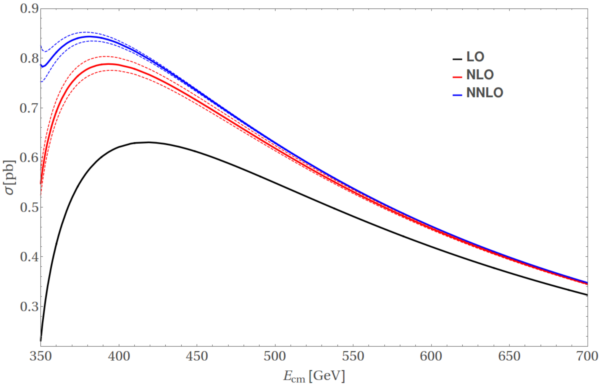
shows our result for the cross section at LO, NLO, and NNLO QCD for c.m. energies (with input values of the SM parameters specified in ref. [39]). In the case of and the solid lines represent the values computed with the choice for the renormalization scale. Uncertainties due to undetermined higher-order corrections are conventionally estimated by varying the renormalization-scale between and . The upper and lower dashed lines correspond to these scale variations. In order to exhibit the size of the higher order QCD corrections relative to the LO cross section, we represent the cross section in the form
| (3.1) |
We list, for a reference, in table 1
| [GeV] | 360 | 381.3 | 400 | 500 |
|---|---|---|---|---|
| 0.627 | 0.352 | 0.266 | 0.127 | |
| 0.281 | 0.110 | 0.070 | 0.020 |
the QCD corrections and for selected c.m. energies for .
From figures 4 we can see that the higher order QCD corrections to the cross sections decrease with increasing c.m. energies after GeV. As clearly shown, in the region where the perturbative calculation is reliable, the scale-variation band at NNLO is narrower than at NLO, as expected in perturbative calculations. Notice also that the scale-variation bands do not overlap here. In the near threshold region, the QCD corrections become rather large. The blue thick line in fig. 4 representing the total NNLO result already shows a hint of blowing up when This is due to the well-known Coulomb singularities [71, 33] in this process. The NLO cross section, i.e., the red line in fig. 4, does not diverge but goes to a constant for , because it involves only a single Coulomb singularity, due to one virtual longitudinal gluon exchange, which is compensated by the suppression factor due to the shrinking phase-space. The presence of Coulomb singularities in fixed order perturbative calculations near threshold clearly signifies the break-down of such a calculation. Within perturbation theory, one way to improve in the near threshold region is to sum up these Coulomb singularities through all perturbative orders, which then leads to a finite result (see, for instance, [71, 72, 42]).
The numbers in table 1 suggest that fixed order perturbation theory can be applied for GeV. In the computation of , we have included also the non-universal contributions of order that contain the electroweak couplings of quarks . These contributions are free of divergences and are very small. For instance, at = 500 GeV they amount to of the total second order correction defined in Eq. (3.1), and this fraction decreases further in magnitude for smaller c.m. energies.
We have numerically compared our exact NNLO result with the expanded results in the near threshold region [73, 74, 75, 76] and in the asymptotic region [32, 33, 34, 35] where , and found agreement. Furthermore, our results shown in table 1 agree with the calculation of the cross section in ref.[38]. For a detailed discussion of our results on differential distributions of the top quark pair prodution we refer to ref. [39].
4 The forward-backward asymmetries in
4.1 Definitions of the un-expanded and expanded
The forward-backward asymmetry in the heavy production, is defined by
| (4.1) |
where is the number of quarks produced in the forward (backward) direction. The asymmetry in the reaction is generated by those terms in the squared S-matrix elements which are odd under the interchange of and while the initial state is kept fixed. The identification of the forward/backward direction involves a choice of reference axis. The definition of the reference axis must be such that the resulting forward-backward asymmetry is an infrared safe (IR-safe) quantity so that it can be reliably calculated and subsequently compared with experimental measurements. Common choices include the direction of flight of the heavy quark and the oriented thrust axis defined by a certain thrust-finding algorithm [77, 78].
The heavy quark forward-backward asymmetry can also be expressed in terms of the symmetric cross section and the antisymmetric cross section for the inclusive production of the heavy quark , i.e.,
| (4.2) |
The and are the forward and backward cross sections, respectively, which can be written in terms of differential cross sections as
| (4.3) |
where is the angle between the electron three-momentum and the axis defining the forward hemisphere. The energy ratio is defined as where is the energy of the heavy quark .
To order the symmetric and antisymmetric cross sections receive the following perturbative contributions:
| (4.4) |
where the first number in the superscripts denotes the number of final-state partons associated with the respective term and the second one the order of . Inserting (4.4) into (4.2) we get the unexpanded to first and to second order in :
| (4.5) | ||||
| (4.6) |
where
| (4.7) |
is the forward-backward asymmetry at Born level. The factors and defined by the respective ratio on the left of eq. (4.5) and (4.6) are the unexpanded first-order and second-order QCD correction factors.
Taylor expanding eq. (4.5) to first order and of (4.6) to second order in gives
| (4.8) | ||||
| (4.9) |
where and are the QCD corrections of and , respectively.
| (4.10) | ||||
| (4.11) |
Eqs. (4.8) and (4.9) are the expanded forms of the forward-backward asymmetry at NLO and NNLO QCD. The unexpanded and expanded first and second-order forward-backward asymmetries differ by terms of order and order , respectively. The differences between the two forms may be considered as an estimate of the theory uncertainties.
4.2 Numerical results for the in the continuum
Table 2 contains our results for the expanded form of the top-quark forward-backward asymmetry at NLO and NNLO QCD defined in eq. (4.8) and (4.9), respectively, and the correction terms and given in Eq. (4.10) and (4.11) for several c.m. energies. The central values and the uncertainties refer to the scales and and , respectively. Obviously, here we vary simultaneously in the and of different partonic channels between and . We note that we have included in also the non-universal contributions that contain the electroweak couplings of quarks .
| [GeV] | [%] | [%] | [%] | [%] | [%] | [%] |
|---|---|---|---|---|---|---|
| 360 | 14.94 | |||||
| 400 | 28.02 | |||||
| 500 | 41.48 | |||||
| 700 | 51.34 |
Table 3 contains our results for the unexpanded form of the top-quark at NLO and NNLO QCD and the associated QCD correction factors and defined in eq. (4.5) and (4.6) for several c.m. energies. This form of computing the asymmetry corresponds to the simulation using Monte-Carlo event generators. The at NNLO QCD was computed before in ref. [38] in the unexpanded form with values of and that differ slightly from the ones that we use here, while the results basically agree.
| [GeV] | [%] | [%] | [%] |
|---|---|---|---|
| 360 | 14.94 | ||
| 400 | 28.02 | ||
| 500 | 41.48 | ||
| 700 | 51.34 |
4.3 Numerical results for the at the resonance
We now present our numerical results on the -quark forward-backward asymmetry at the resonance to in QCD and lowest order in the electroweak couplings. The input values of the SM couplings and masses are specified in detail in ref. [46]. In particular, we use defined in the 5-flavor QCD and the bottom-quark on-shell mass GeV. For the mass of the top quark that appears in the triangle-loop diagrams contributing to the non-universal corrections to we use GeV. The quarks are taken to be massless. With these input parameters, the Born-level value of the -quark forward-backward asymmetry at is . The value of is very sensitive to the input value of but insensitive to the value of within its uncertainty. Here, we discuss only the results of the QCD corrections for the expanded with respect to both the -quark and the thrust direction, the later of which enters the subsequent discussion of the phenomenological consequences. Table 4 lists the values of the NLO and NNLO correction factor, both for the quark axis and the thrust axis definition, for the three renormalization scales . The numbers given in this table show that the order corrections are significant. For the ratio is and for the quark and thrust axis definition, respectively. The scale variations change both the first- and second-order QCD correction factors by about with respect to their values at . The fact that inclusion of the second-order correction term does not reduce the scale uncertainty is not unusual for an observable that is defined as a ratio. Contrary to the case of the top quark for the c.m. energies below the threshold, the order and corrections and are dominated by the contributions from the three-parton and three- and four-parton final states, respectively. We have included in the computation of the non-universal corrections of order that contain the vector and axial vector couplings of quarks , which turn out to be quite sizable. We note that the non-universal corrections depend on the value of .
4.4 Phenomenological consequences
The with QCD corrections calculated above cannot be compared directly with experimental measurements. In the measurements of the -quark asymmetry by the experiments at the previous colliders LEP and SLAC, which are reviewed in [1, 79, 80], the forward and backward hemispheres was defined using the thrust axis. In our computation the thrust axis is used but identified only for partonic final states, while the hadronization of partons causes a smearing of this axis (causing discrepancy between thrust at the parton level and at the level of stable hadrons). Results from several experimental measurements with different acceptance regions in phase space, and different sensitivity to QCD-correction effects etc, are combined after unfolded respectively. Bearing this in mind, we proceed with the analysis as described in ref. [46], which, albeit being very preliminary and far from full-fledged, can give a quick idea about what might be the possible consequence of a revised QCD-correction factor 22 2 See ref. [81] for an updated analysis of the theoretical uncertainties.. In short, a pseudo-observable, the bare -quark asymmetry , is extracted from the measured asymmetry [82, 83] in the following way. The the measured asymmetry was first corrected for QCD effects as follows,
| (4.12) |
and then the QCD corrected “experimental” asymmetry was further corrected for higher order electroweak corrections etc, before a value of the bare asymmetry was deduced:
| (4.13) |
The corrections include the energy shift from GeV (all measured asymmetries were corrected, in a first step, to this energy) to , QED corrections, corrections due to exchange and interference, and due to imaginary parts of effective weak couplings (cf. for instance, [27]). In this way, the experimental value determined for this pseudo-observable reads as and shows a large deviation, about , from the SM fit [1, 80] if the NNLO QCD corrections for massless quarks are used.
The QCD correction factor determined in [82] is where the error includes estimates of hadronization effects. Our thrust axis correction factor where the error is due to scale uncertainties only, agrees with that factor within the uncertainties. Our central value is smaller than by , and accordingly our correction changes the value of the pseudo-observable to . Thus the pull between and the SM fit cited above is slightly decreased, namely from to .
The fixed-order results discussed above were determined at the conventional scale choice . Due to the missing higher order perturbative corrections, the truncated fixed order results on still have a remaining dependence. One way to improve the perturbative result regarding this aspect is to resum all explicit terms in that are related the QCD function, absorbed into a new effective coupling for this particular observable, by means of the well-known optimization procedure based on the Principle of Maximum Conformality (PMC). Following the PMC procedure we determined the PMC scale to be for the quark forward-backward asymmetry with the thrust axis definition in ref. [47]. After applying PMC scale setting, the QCD correction factor with the thrust axis definition is , which is smaller than by . Consequently, the QCD correction factor with refinements from the PMC method changes to
| (4.14) |
which shows a deviation from the SM fit .
It is noted that there are updated SM fit results reported in refs. [10, 11] with improved electroweak corrections taken into account. To see more clearly how the deviations are changed due to the incorporation of updated electroweak and QCD corrections, in table (5), we list the deviations computed using different central values of the SM fit , and also the determined by making use of the different parton-level QCD correction factors.
| v.s. | 0.0992 ref. [80] | 0.0996 ref. [46] | 1.004 ref. [47] |
|---|---|---|---|
| 0.1038 ref. [1] | 2.9 | 2.6 | 2.1 |
| 0.1032 ref. [10] | 2.5 | 2.25 | 1.8 |
| 0.1030 ref. [11] | 2.4 | 2.1 | 1.6 |
So far the tension between and seems to decrease progressively over the years. However, the experimental uncertainty of measurement used in determining the numbers in this table is still the one at the SLAC and LEP experiments, about [1]. On the other hand, the experimental uncertainty, currently dominated by the statistical uncertainties, is expected to be greatly reduced at future lepton colliders [12, 13, 15, 16, 14]. Confirmation or resolution of this long-term discrepancy at the future lepton colliders would, of course, make a great impact on the development of our theories.
5 Conclusions
We have formulated a set-up for computing the production of a heavy quark-antiquark pair in collisions at in the perturbative QCD at the differential level, using the antenna subtraction method for handling the intermediate infrared soft and collinear divergences of the individual contributions. This set-up applies to the differential calculation of any infrared-safe observable of this process to in QCD, and works in a numerically stable way owing to the local subtraction of IR divergences in each partonic phase space.
Besides the application to pair production at (future) collisions, we have determined the QCD corrections to the b-quark forward-backward asymmetry in collisions at the resonance, aimed at analysing the long-standing tension between its direct determination at the SLAC and LEP experiments and its global SM fit. We found that after taking into account exact b-quark mass effects, the pull between the direct determination of and its SM fit is reduced from 2.9 to 2.6. Furthermore, we performed an improved determination of this QCD correction factor by means of the optimization procedure based on the Principle of Maximum Conformality, with which the tension is eventually reduced down to 2.1. Once compared to the updated SM-fit results, the deviation gets reduced below 2. As a future application of our computational set-up, one may consider the determination of the corrections to the forward-backward asymmetry for two -jet final states, for which one expects a decrease of the magnitude of the QCD corrections. Furthermore, this setup can be applied to the prodution of polarized top quarks, with polarized beams.
Acknowledgments
The author is grateful to Werner Bernreuther, Oliver Dekkers, Thomas Gehrmann, Dennis Heisler, Rui-qing Meng, Jian-ming Shen, Zong-guo Si, Sheng-quan Wang, Xing-gang Wu for collaborating on the work presented in this proceeding.
References
- [1] SLD Electroweak Group, DELPHI, ALEPH, SLD, SLD Heavy Flavour Group, OPAL, LEP Electroweak Working Group, L3 Collaboration, S. Schael et al., Precision electroweak measurements on the resonance, Phys. Rept. 427 (2006) 257–454, arXiv:hep-ex/0509008 [hep-ex].
- [2] ALEPH, CDF, D0, DELPHI, L3, OPAL, SLD, LEP Electroweak Working Group, Tevatron Electroweak Working Group, SLD Electroweak Working Group, SLD Heavy Flavor Group Collaboration, Precision Electroweak Measurements and Constraints on the Standard Model, arXiv:0911.2604 [hep-ex].
- [3] ECFA/DESY LC Physics Working Group Collaboration, J. A. Aguilar-Saavedra et al., TESLA: The Superconducting electron positron linear collider with an integrated x-ray laser laboratory. Technical design report. Part 3. Physics at an linear collider, arXiv:hep-ph/0106315 [hep-ph].
- [4] H. Baer, T. Barklow, K. Fujii, Y. Gao, A. Hoang, S. Kanemura, J. List, H. E. Logan, A. Nomerotski, M. Perelstein, et al., The International Linear Collider Technical Design Report - Volume 2: Physics, arXiv:1306.6352 [hep-ph].
- [5] TLEP Design Study Working Group Collaboration, M. Bicer et al., First Look at the Physics Case of TLEP, JHEP 01 (2014) 164, arXiv:1308.6176 [hep-ex].
- [6] L. Linssen, A. Miyamoto, M. Stanitzki, and H. Weerts, Physics and Detectors at CLIC: CLIC Conceptual Design Report, arXiv:1202.5940 [physics.ins-det].
- [7] FCC Collaboration, A. Abada et al., FCC-ee: The Lepton Collider: Future Circular Collider Conceptual Design Report Volume 2, Eur. Phys. J. ST 228 no. 2, (2019) 261–623.
- [8] M. Ahmad et al., CEPC-SPPC Preliminary Conceptual Design Report. 1. Physics and Detector, .
- [9] CEPC-SPPC Preliminary Conceptual Design Report. 2. Accelerator, .
- [10] Gfitter Group Collaboration, M. Baak, J. Cuth, J. Haller, A. Hoecker, R. Kogler, K. Moenig, M. Schott, and J. Stelzer, The global electroweak fit at NNLO and prospects for the LHC and ILC, Eur. Phys. J. C74 (2014) 3046, arXiv:1407.3792 [hep-ph].
- [11] Particle Data Group Collaboration, M. Tanabashi et al., Review of Particle Physics, Phys. Rev. D98 no. 3, (2018) 030001.
- [12] R. Hawkings and K. Monig, Electroweak and CP violation physics at a linear collider factory, Eur. Phys. J.direct C1 (1999) 8, arXiv:hep-ex/9910022 [hep-ex].
- [13] J. Erler, S. Heinemeyer, W. Hollik, G. Weiglein, and P. M. Zerwas, Physics impact of GigaZ, Phys. Lett. B486 (2000) 125–133.
- [14] ILD Concept Group Collaboration, H. Abramowicz et al., International Large Detector: Interim Design Report, arXiv:2003.01116 [physics.ins-det].
- [15] E. Devetak, A. Nomerotski, and M. Peskin, Top quark anomalous couplings at the International Linear Collider, Phys. Rev. D84 (2011) 034029, arXiv:1005.1756 [hep-ex].
- [16] M. S. Amjad, M. Boronat, T. Frisson, I. Garcia, R. Poschl, E. Ros, F. Richard, J. Rouene, P. R. Femenia, and M. Vos, A precise determination of top quark electro-weak couplings at the ILC operating at GeV, arXiv:1307.8102 [hep-ex].
- [17] J. Jersak, E. Laermann, and P. M. Zerwas, Electroweak Production of Heavy Quarks in Annihilation, Phys. Rev. D25 (1982) 1218. [Erratum: Phys. Rev.D36,310(1987)].
- [18] W. Bernreuther, A. Brandenburg, and P. Uwer, Next-to-leading order QCD corrections to three jet cross-sections with massive quarks, Phys. Rev. Lett. 79 (1997) 189–192, arXiv:hep-ph/9703305 [hep-ph].
- [19] A. Brandenburg and P. Uwer, Next-to-leading order QCD corrections and massive quarks in three jets, Nucl. Phys. B515 (1998) 279–320, arXiv:hep-ph/9708350 [hep-ph].
- [20] G. Rodrigo, A. Santamaria, and M. S. Bilenky, Do the quark masses run? Extracting from LEP data, Phys. Rev. Lett. 79 (1997) 193–196, arXiv:hep-ph/9703358 [hep-ph].
- [21] G. Rodrigo, M. S. Bilenky, and A. Santamaria, Quark mass effects for jet production in collisions at the next-to-leading order: Results and applications, Nucl. Phys. B554 (1999) 257–297, arXiv:hep-ph/9905276 [hep-ph].
- [22] P. Nason and C. Oleari, Next-to-leading order corrections to momentum correlations in , Phys. Lett. B407 (1997) 57–60, arXiv:hep-ph/9705295 [hep-ph].
- [23] P. Nason and C. Oleari, Next-to-leading order corrections to the production of heavy flavor jets in collisions, Nucl. Phys. B521 (1998) 237–273, arXiv:hep-ph/9709360 [hep-ph].
- [24] W. Beenakker, S. C. van der Marck, and W. Hollik, annihilation into heavy fermion pairs at high-energy colliders, Nucl. Phys. B365 (1991) 24–78.
- [25] M. Bohm et al., FORWARD - BACKWARD ASYMMETRIES, in LEP Physics Workshop. 9, 1989.
- [26] D. Yu. Bardin, P. Christova, M. Jack, L. Kalinovskaya, A. Olchevski, S. Riemann, and T. Riemann, ZFITTER v.6.21: A Semianalytical program for fermion pair production in annihilation, Comput. Phys. Commun. 133 (2001) 229–395, arXiv:hep-ph/9908433 [hep-ph].
- [27] A. Freitas and K. Monig, Corrections to quark asymmetries at LEP, Eur. Phys. J. C40 (2005) 493, arXiv:hep-ph/0411304 [hep-ph].
- [28] J. Fleischer, A. Leike, T. Riemann, and A. Werthenbach, Electroweak one loop corrections for annihilation into t anti-top including hard bremsstrahlung, Eur. Phys. J. C31 (2003) 37–56, arXiv:hep-ph/0302259 [hep-ph].
- [29] T. Hahn, W. Hollik, A. Lorca, T. Riemann, and A. Werthenbach, electroweak corrections to the processes : A Comparison, in Proceedings, 4th ECFA / DESY Workshop on Physics and Detectors for a 90-GeV to 800-GeV Linear Collider: Amsterdam, Netherlands, April 1-4, 2003. 2003. arXiv:hep-ph/0307132 [hep-ph]. http://inspirehep.net/record/623116/files/arXiv:hep-ph_0307132.pdf.
- [30] P. H. Khiem, J. Fujimoto, T. Ishikawa, T. Kaneko, K. Kato, Y. Kurihara, Y. Shimizu, T. Ueda, J. A. M. Vermaseren, and Y. Yasui, Full electroweak radiative corrections to with GRACE-Loop, Eur. Phys. J. C73 no. 4, (2013) 2400, arXiv:1211.1112 [hep-ph].
- [31] J. Blümlein, A. De Freitas, and K. Schönwald, The QED initial state corrections to the forward-backward asymmetry of to higher orders, Phys. Lett. B 816 (2021) 136250, arXiv:2102.12237 [hep-ph].
- [32] S. G. Gorishnii, A. L. Kataev, and S. A. Larin, Three Loop Corrections of Order to the Correlator of Electromagnetic Quark Currents, Nuovo Cim. A92 (1986) 119–131.
- [33] K. G. Chetyrkin, J. H. Kuhn, and M. Steinhauser, Three loop polarization function and corrections to the production of heavy quarks, Nucl. Phys. B482 (1996) 213–240, arXiv:hep-ph/9606230 [hep-ph].
- [34] K. G. Chetyrkin, R. Harlander, J. H. Kuhn, and M. Steinhauser, Mass corrections to the vector current correlator, Nucl. Phys. B503 (1997) 339–353, arXiv:hep-ph/9704222 [hep-ph].
- [35] K. G. Chetyrkin, A. H. Hoang, J. H. Kuhn, M. Steinhauser, and T. Teubner, Massive quark production in electron positron annihilation to order , Eur. Phys. J. C2 (1998) 137–150, arXiv:hep-ph/9711327 [hep-ph].
- [36] Y. Kiyo, A. Maier, P. Maierhofer, and P. Marquard, Reconstruction of heavy quark current correlators at , Nucl. Phys. B823 (2009) 269–287, arXiv:0907.2120 [hep-ph].
- [37] J. Gao and H. X. Zhu, Electroweak prodution of top-quark pairs in annihilation at NNLO in QCD: the vector contributions, Phys. Rev. D90 no. 11, (2014) 114022, arXiv:1408.5150 [hep-ph].
- [38] J. Gao and H. X. Zhu, Top Quark Forward-Backward Asymmetry in Annihilation at Next-to-Next-to-Leading Order in QCD, Phys. Rev. Lett. 113 no. 26, (2014) 262001, arXiv:1410.3165 [hep-ph].
- [39] L. Chen, O. Dekkers, D. Heisler, W. Bernreuther, and Z.-G. Si, Top-quark pair production at next-to-next-to-leading order QCD in electron positron collisions, arXiv:1610.07897 [hep-ph].
- [40] D. A. Kosower, Antenna factorization in strongly ordered limits, Phys. Rev. D71 (2005) 045016, arXiv:hep-ph/0311272 [hep-ph].
- [41] A. Gehrmann-De Ridder, T. Gehrmann, and E. W. N. Glover, Antenna subtraction at NNLO, JHEP 09 (2005) 056, arXiv:hep-ph/0505111 [hep-ph].
- [42] M. Beneke, Y. Kiyo, P. Marquard, A. Penin, J. Piclum, and M. Steinhauser, Next-to-Next-to-Next-to-Leading Order QCD Prediction for the Top Antitop -Wave Pair Production Cross Section Near Threshold in Annihilation, Phys. Rev. Lett. 115 no. 19, (2015) 192001, arXiv:1506.06864 [hep-ph].
- [43] V. Ravindran and W. L. van Neerven, Second order QCD corrections to the forward - backward asymmetry in collisions, Phys. Lett. B445 (1998) 214–222, arXiv:hep-ph/9809411 [hep-ph].
- [44] S. Catani and M. H. Seymour, Corrections of to the forward backward asymmetry, JHEP 07 (1999) 023, arXiv:hep-ph/9905424 [hep-ph].
- [45] S. Weinzierl, The Forward-backward asymmetry at NNLO revisited, Phys. Lett. B644 (2007) 331–335, arXiv:hep-ph/0609021 [hep-ph].
- [46] W. Bernreuther, L. Chen, O. Dekkers, T. Gehrmann, and D. Heisler, The forward-backward asymmetry for massive bottom quarks at the peak at next-to-next-to-leading order QCD, JHEP 01 (2017) 053, arXiv:1611.07942 [hep-ph].
- [47] S.-Q. Wang, R.-Q. Meng, X.-G. Wu, L. Chen, and J.-M. Shen, Revisiting the bottom quark forward–backward asymmetry in electron–positron collisions, Eur. Phys. J. C 80 no. 7, (2020) 649, arXiv:2003.13941 [hep-ph].
- [48] W. Bernreuther, R. Bonciani, T. Gehrmann, R. Heinesch, T. Leineweber, P. Mastrolia, and E. Remiddi, Two-loop QCD corrections to the heavy quark form-factors: The Vector contributions, Nucl. Phys. B706 (2005) 245–324, arXiv:hep-ph/0406046 [hep-ph].
- [49] W. Bernreuther, R. Bonciani, T. Gehrmann, R. Heinesch, T. Leineweber, P. Mastrolia, and E. Remiddi, Two-loop QCD corrections to the heavy quark form-factors: Axial vector contributions, Nucl. Phys. B712 (2005) 229–286, arXiv:hep-ph/0412259 [hep-ph].
- [50] W. Bernreuther, R. Bonciani, T. Gehrmann, R. Heinesch, T. Leineweber, and E. Remiddi, Two-loop QCD corrections to the heavy quark form-factors: Anomaly contributions, Nucl. Phys. B723 (2005) 91–116, arXiv:hep-ph/0504190 [hep-ph].
- [51] D. A. Kosower, Antenna factorization of gauge theory amplitudes, Phys. Rev. D57 (1998) 5410–5416, arXiv:hep-ph/9710213 [hep-ph].
- [52] S. J. Parke and T. R. Taylor, An Amplitude for Gluon Scattering, Phys. Rev. Lett. 56 (1986) 2459.
- [53] M. L. Mangano, S. J. Parke, and Z. Xu, Duality and Multi - Gluon Scattering, Nucl. Phys. B298 (1988) 653–672.
- [54] F. A. Berends and W. Giele, The Six Gluon Process as an Example of Weyl-Van Der Waerden Spinor Calculus, Nucl. Phys. B294 (1987) 700–732.
- [55] F. A. Berends and W. T. Giele, Multiple Soft Gluon Radiation in Parton Processes, Nucl. Phys. B313 (1989) 595–633.
- [56] M. L. Mangano and S. J. Parke, Multiparton amplitudes in gauge theories, Phys. Rept. 200 (1991) 301–367, arXiv:hep-th/0509223 [hep-th].
- [57] J. M. Campbell and E. W. N. Glover, Double unresolved approximations to multiparton scattering amplitudes, Nucl. Phys. B527 (1998) 264–288, arXiv:hep-ph/9710255 [hep-ph].
- [58] Z. Bern, V. Del Duca, W. B. Kilgore, and C. R. Schmidt, The infrared behavior of one loop QCD amplitudes at next-to-next-to leading order, Phys. Rev. D60 (1999) 116001, arXiv:hep-ph/9903516 [hep-ph].
- [59] D. A. Kosower, All order collinear behavior in gauge theories, Nucl. Phys. B552 (1999) 319–336, arXiv:hep-ph/9901201 [hep-ph].
- [60] A. Gehrmann-De Ridder, T. Gehrmann, and G. Heinrich, Four particle phase space integrals in massless QCD, Nucl. Phys. B682 (2004) 265–288, arXiv:hep-ph/0311276 [hep-ph].
- [61] A. Gehrmann-De Ridder and M. Ritzmann, NLO Antenna Subtraction with Massive Fermions, JHEP 07 (2009) 041, arXiv:0904.3297 [hep-ph].
- [62] G. Abelof and A. Gehrmann-De Ridder, Antenna subtraction for the production of heavy particles at hadron colliders, JHEP 04 (2011) 063, arXiv:1102.2443 [hep-ph].
- [63] G. Abelof and A. Gehrmann-De Ridder, Double real radiation corrections to production at the LHC: the all-fermion processes, JHEP 04 (2012) 076, arXiv:1112.4736 [hep-ph].
- [64] G. Abelof, O. Dekkers, and A. Gehrmann-De Ridder, Antenna subtraction with massive fermions at NNLO: Double real initial-final configurations, JHEP 12 (2012) 107, arXiv:1210.5059 [hep-ph].
- [65] G. Abelof, A. Gehrmann-De Ridder, P. Maierhofer, and S. Pozzorini, NNLO QCD subtraction for top-antitop production in the channel, JHEP 08 (2014) 035, arXiv:1404.6493 [hep-ph].
- [66] G. Abelof and A. Gehrmann-De Ridder, Light fermionic NNLO QCD corrections to top-antitop production in the quark-antiquark channel, JHEP 12 (2014) 076, arXiv:1409.3148 [hep-ph].
- [67] G. Abelof, A. Gehrmann-De Ridder, and I. Majer, Top quark pair production at NNLO in the quark-antiquark channel, JHEP 12 (2015) 074, arXiv:1506.04037 [hep-ph].
- [68] W. Bernreuther, C. Bogner, and O. Dekkers, The real radiation antenna function for at NNLO QCD, JHEP 06 (2011) 032, arXiv:1105.0530 [hep-ph].
- [69] W. Bernreuther, C. Bogner, and O. Dekkers, The real radiation antenna functions for at NNLO QCD, JHEP 10 (2013) 161, arXiv:1309.6887 [hep-ph].
- [70] O. Dekkers and W. Bernreuther, The real-virtual antenna functions for at NNLO QCD, Phys. Lett. B738 (2014) 325–333, arXiv:1409.3124 [hep-ph].
- [71] B. H. Smith and M. B. Voloshin, at the threshold and beyond, Phys. Lett. B324 (1994) 117–120, arXiv:hep-ph/9312358 [hep-ph]. [Erratum: Phys. Lett.B333,564(1994)].
- [72] N. Brambilla, A. Pineda, J. Soto, and A. Vairo, Effective field theories for heavy quarkonium, Rev. Mod. Phys. 77 (2005) 1423, arXiv:hep-ph/0410047 [hep-ph].
- [73] A. Czarnecki and K. Melnikov, Two loop QCD corrections to the heavy quark pair production cross-section in annihilation near the threshold, Phys. Rev. Lett. 80 (1998) 2531–2534, arXiv:hep-ph/9712222 [hep-ph].
- [74] M. Beneke, A. Signer, and V. A. Smirnov, Two loop correction to the leptonic decay of quarkonium, Phys. Rev. Lett. 80 (1998) 2535–2538, arXiv:hep-ph/9712302 [hep-ph].
- [75] A. H. Hoang, Two loop corrections to the electromagnetic vertex for energies close to threshold, Phys. Rev. D56 (1997) 7276–7283, arXiv:hep-ph/9703404 [hep-ph].
- [76] W. Bernreuther, R. Bonciani, T. Gehrmann, R. Heinesch, T. Leineweber, P. Mastrolia, and E. Remiddi, Two-Parton Contribution to the Heavy-Quark Forward-Backward Asymmetry in NNLO QCD, Nucl. Phys. B750 (2006) 83–107, arXiv:hep-ph/0604031 [hep-ph].
- [77] E. Farhi, A QCD Test for Jets, Phys. Rev. Lett. 39 (1977) 1587–1588.
- [78] S. Brandt, C. Peyrou, R. Sosnowski, and A. Wroblewski, The Principal axis of jets. An Attempt to analyze high-energy collisions as two-body processes, Phys. Lett. 12 (1964) 57–61.
- [79] Tevatron Electroweak Working Group, CDF, SLD Heavy Flavor Group, DELPHI, ALEPH, SLD Electroweak Working Group, LEP Electroweak Working Group, SLD, OPAL, D0, L3 Collaboration, J. Alcaraz et al., Precision Electroweak Measurements and Constraints on the Standard Model, arXiv:0911.2604 [hep-ex].
- [80] Tevatron Electroweak Working Group, CDF, DELPHI, SLD Electroweak and Heavy Flavour Groups, ALEPH, LEP Electroweak Working Group, SLD, OPAL, D0, L3 Collaboration, L. E. W. Group, Precision Electroweak Measurements and Constraints on the Standard Model, arXiv:1012.2367 [hep-ex].
- [81] D. d’Enterria and C. Yan, Revised QCD effects on the Z forward-backward asymmetry, arXiv:2011.00530 [hep-ph].
- [82] D. Abbaneo et al., LEP/SLD heavy flavour working group: Final Input Parameters for the LEP/SLD Heavy Flavour Analyses, http://lepewwg.web.cern.ch/LEPEWWG/heavy/ (2001) .
- [83] LEP Heavy Flavor Working Group Collaboration, D. Abbaneo, P. Antilogus, T. Behnke, S. C. Blyth, M. Elsing, R. Faccini, R. W. L. Jones, K. Monig, S. Petzold, and R. Tenchini, QCD corrections to the forward - backward asymmetries of c and b quarks at the Z pole, Eur. Phys. J. C4 (1998) 185–191.