跳到论文正文
W Papers独立论文阅读器 arXiv:2105.06207 论文正文 计算阅读时间 · 0%
引用这篇论文根据当前论文元数据生成,正式投稿前建议核对。


License: CC BY 4.0
arXiv:2105.06207v1 [hep-ph] 13 May 2021

Up-down Asymmetries and Angular Distributions in D→K1(→Kππ)ℓ+νℓD\to K_{1}(\to K\pi\pi)\ell^{+}\nu_{\ell}

Lingzhu Bian 1, Liang Sun 1, Wei Wang 2 Affiliation: 1 School of Physics and Technology, Wuhan University, Wuhan, China
2 INPAC, Key Laboratory for Particle Astrophysics and Cosmology (MOE), Shanghai Key Laboratory for Particle Physics and Cosmology, School of Physics and Astronomy, Shanghai Jiao Tong University, Shanghai 200240, China
Abstract

Using the helicity amplitude technique, we derive differential decay widths and angular distributions for the decay cascade D→K1​(1270,1400)​ℓ+​νℓ→(K​π​π)​ℓ+​νℓ​(ℓ=e,μ)D\to K_{1}(1270,1400)\ell^{+}\nu_{\ell}\to(K\pi\pi)\ell^{+}\nu_{\ell}(\ell=e,\mu), in which the electron and muon mass is explicitly included. Using a set of phenomenological results for D→K1D\to K_{1} form factors, we calculate partial decay widths and branching fractions for D0→K1−​ℓ+​νℓD^{0}\to K_{1}^{-}\ell^{+}\nu_{\ell} and D+→K10​ℓ+​νℓD^{+}\to K_{1}^{0}\ell^{+}\nu_{\ell}, but find that results for ℬ⁡(D→K1​(1270)​e+​νe){\cal B}(D\to K_{1}(1270)e^{+}\nu_{e}) are larger than recent BESIII measurements by about a factor 1.5. We further demonstrate that the measurement of up-down asymmetry in D→K1​e+​νe→(K​π​π)​e+​νeD\to K_{1}e^{+}\nu_{e}\to(K\pi\pi)e^{+}\nu_{e} and angular distributions in D→K1​ℓ+​νℓ→(K​π​π)​ℓ+​νℓD\to K_{1}\ell^{+}\nu_{\ell}\to(K\pi\pi)\ell^{+}\nu_{\ell} can help to determine the hadronic amplitude requested in B→K1(→Kππ)γB\to K_{1}(\to K\pi\pi)\gamma. Based on the Monte-Carlo simulation with the LHCb geometrical acceptance, we find that the angular distributions of MC events can be well described.

I Introduction

Since the establishment of standard model (SM) in 1960s, searching for new physics (NP) beyond SM has become a most primary objective in particle physics. This can in principle proceed in two distinct directions. It is likely that new particles emerge directly in high energy collisions for instance at large hadron collider (LHC). On the other side, NP particles can affect various low-energy observables by modifying the coupling strength or introducing new interaction forms and thus a high precision study of these observables is likely to indirectly access the NP. In the SM, the charged weak interaction has the V−AV-A chirality and thereby the photon in b→s​γb\to s\gamma is predominantly left-handed. The contribution with right-handed polarization is suppressed by the ratio of strange and bottom quark masses. Therefore the measurement of photon polarization in b→s​γb\to s\gamma provides a unique probe for new physics Atwood:1997zr; Becirevic:2012dx; Paul:2016urs. A representative scenario of this type is the left-right symmetric model Kou:2013gna; Haba:2015gwa, in which the photon can acquire a significant right-handed component.

In practice, the chirality of the b→s​γb\to s\gamma can be detected using the measurements of inclusive B→Xs​γB\to X_{s}\gamma decay branching fractions Aubert:2007my; Lees:2012ym; Lees:2012wg; Saito:2014das, the mixing-induced C​PCP asymmetries of radiative B0B^{0} and Bs0B_{s}^{0} decays Ushiroda:2006fi; Aubert:2008gy; Aaij:2019pnd; Akar:2018zhv and the B→K∗​e+​e−B\to K^{*}e^{+}e^{-} with very low dilepton mass squared Grossman:2000rk; Aaij:2020umj. Interestingly, the photon helicity in radiative DD decays was also explored deBoer:2018zhz.

In addition to the above methods, it is pointed out that the photon helicity in b→s​γb\to s\gamma is proportional to an up-down asymmetry 𝒜UD\mathcal{A}_{\rm UD} in B→K1(→Kππ)γB\to K_{1}(\to K\pi\pi)\gamma Gronau:2001ng; Gronau:2002rz; Kou:2010kn and more generally the angular distribution in B→Kr​e​s(→Kππ)γB\to K_{res}(\to K\pi\pi)\gamma. Throughout this work we will use K1K_{1} to abbreviate the axial-vector meson K1​(1270)K_{1}(1270) and/or K1​(1400)K_{1}(1400). However the measurement of up-down asymmetry in B→K1​γB\to K_{1}\gamma Aaij:2014wgo alone was incapable to reveal the photon helicity due to the entanglement with the K1K_{1} decay dynamics. Many interesting theoretical analyses have adopted nonperturbative approaches to parametrize the K1→K​π​πK_{1}\to K\pi\pi decay amplitude and power constraints on the decay parameters were obtained Gronau:2001ng; Gronau:2002rz; Kou:2010kn; Tayduganov:2011ui; Gronau:2017kyq. In a previous work Wang:2019wee it is proposed that one can tackle this problem by combining semileptonic D→K1​e+​νeD\to K_{1}e^{+}\nu_{e} decays. In particular, a ratio of up-down asymmetries in D→K1(→Kππ)e+νeD\to K_{1}(\to K\pi\pi)e^{+}\nu_{e}, 𝒜U​D′{\cal A}_{UD}^{\prime}, has been proposed to quantify the hadronic effects in K1→K​π​πK_{1}\to K\pi\pi decay. More explicitly the photon helicity can be expressed as a ratio of the two observables λγ=3/4×𝒜U​D/𝒜UD′\lambda_{\gamma}=3/4\times{\cal A}_{UD}/\mathcal{A}_{\rm UD}^{\prime} Wang:2019wee.

The purpose of this work is multifold. We will first give the details in the helicity amplitude approach to derive the pertinent angular distributions and up-down asymmetries. Secondly we will extend the previous analysis to the muon mode whose mass can not be neglected in DD decays. Using the phenomenological results for D→K1D\to K_{1} form factors, we calculate partial decay widths for D→K1​ℓ+​νℓD\to K_{1}\ell^{+}\nu_{\ell}, and show that the measurement of up-down asymmetry in D→K1(→Kππ)e+νeD\to K_{1}(\to K\pi\pi)e^{+}\nu_{e} and the angular distribution in D→K1(→Kππ)ℓ+νℓD\to K_{1}(\to K\pi\pi)\ell^{+}\nu_{\ell} can help to determine the hadronic amplitude requested in B→K1(→Kππ)γB\to K_{1}(\to K\pi\pi)\gamma. Based on the Monte Carlo (MC) simulation with the LHCb geometrical acceptance, we find that the angular distributions of MC events can be well described.

The rest of this paper is organized as follows. In Sec. II, we will give a detailed derivation of the angular distributions. In Sec. III, we will use the D→K1D\to K_{1} form factors and calculate the differential decay widths. A comparison of predicted branching fractions with BESIII measurements is made, and a MC simulation of angular distributions with the LHCb geometrical acceptance is also presented. The last section contains a brief summary.

II Framework and Angular Distributions

In this section we will make use of the helicity amplitude technique and derive the angular distributions for the decay cascade D→K1​ℓ+​νℓ→(K​π​π)​ℓ+​νℓD\to K_{1}\ell^{+}\nu_{\ell}\to(K\pi\pi)\ell^{+}\nu_{\ell}. Here the DD and K1K_{1} could be charged or neutral. Since a neutral π0\pi^{0} is difficult to reconstruct especially at hadron colliders, it is more plausible to explore the π+​π−\pi^{+}\pi^{-} final state. Thus we will mainly consider the decay chain D0→K1−​ℓ+​ν→(K−​π+​π−)​ℓ+​νℓD^{0}\to K_{1}^{-}\ell^{+}\nu\to(K^{-}\pi^{+}\pi^{-})\ell^{+}\nu_{\ell} and D+→K¯10​ℓ+​ν→(K¯0​π+​π−)​ℓ+​νℓD^{+}\to\overline{K}_{1}^{0}\ell^{+}\nu\to(\overline{K}^{0}\pi^{+}\pi^{-})\ell^{+}\nu_{\ell}, though the results are also applicable to other decay channels with neutral pions. The kinematics of this decay cascade is shown in Fig. 1. In the lepton pair ℓ+​νℓ\ell^{+}\nu_{\ell} rest frame, θℓ\theta_{\ell} is defined by the ℓ+\ell^{+} flight direction and the opposite of the DD meson flight direction. In K1K_{1} rest frame, n→\vec{n} is defined as the normal direction of the decay plane, and θK\theta_{K} is the relative angle between n→\vec{n} and the opposite of the DD meson flight direction.

A few remarks on the kinematics are given in order.

  • •

    The normal direction is not unambiguous. For instance, in K1−K_{1}^{-} decay plane, it is likely to construct the normal direction with the momentum of π+\pi^{+} and π−\pi^{-}, while the LHCb measurement of up-down asymmetry and angular distributions in B→K1​γB\to K_{1}\gamma makes use of the slow and fast pion momentum Aaij:2014wgo, n→∼p→π,slow×p→π,fast\vec{n}\sim\vec{p}_{\pi,{\rm slow}}\times\vec{p}_{\pi,{\rm fast}}.

  • •

    Secondly, under parity transformation, the DD flight direction will be reversed, but since n→\vec{n} is a cross product of two momenta, its direction is unchanged. Accordingly the θK\theta_{K} will be changed to π−θK\pi-\theta_{K} under parity transformation, implying that the cos⁡θK\cos\theta_{K} is parity odd. The left-handed and right-handed polarization of K1K_{1} gives opposite contributions to the cos⁡θK\cos\theta_{K} term.

  • •

    Thirdly, weak interaction in W∗→ℓ+​νℓW^{*}\to\ell^{+}\nu_{\ell} violates parity conservation. Thus even though cos⁡θℓ\cos\theta_{\ell} is parity-even, the left-handed and right-handed contributions to the cos⁡θℓ\cos\theta_{\ell} term also differ in sign.

  • •

    Furthermore the definition of θK\theta_{K} depends on charge or flavor of K1K_{1}, namely the angle θK\theta_{K} defined in K1−K_{1}^{-} decay may differ with the one defined in K1+K_{1}^{+} system. It is important to stick with the same convention on the kinematics in analyzing BB and DD decays.

Refer to caption
Figure 1: The kinematics for D→K1​ℓ+​νℓ→(K​π​π)​ℓ+​νℓD\to K_{1}\ell^{+}\nu_{\ell}\to(K\pi\pi)\ell^{+}\nu_{\ell}. In the lepton pair ℓ+​νℓ\ell^{+}\nu_{\ell} rest frame, the angle θℓ\theta_{\ell} is defined by the ℓ+\ell^{+} flight direction and the opposite of the DD meson flight direction. In the K1K_{1} rest frame the n→\vec{n} is defined as the normal direction of the K1K_{1} decay plane, and θK\theta_{K} is the relative angle between n→\vec{n} and the opposite of the DD flight direction. Under parity transformation, the DD flight direction will be reversed, but since n→\vec{n} is a cross product of two momenta, its direction is unchanged. Accordingly the θK\theta_{K} will be changed to π−θK\pi-\theta_{K} under parity transformation, implying that the cos⁡θK\cos\theta_{K} is parity odd.

Semileptonic decays of DD into K1K_{1} are induced by effective electro-weak Hamiltonian:

ℋ=GF2​Vc​s​s¯​γμ​(1−γ5)​c×ν¯ℓ​γμ​(1−γ5)​ℓ,\displaystyle{\cal H}=\frac{G_{F}}{\sqrt{2}}V_{cs}\bar{s}\gamma^{\mu}(1-\gamma_{5})c\times\bar{\nu}_{\ell}\gamma_{\mu}(1-\gamma_{5})\ell, (1)

where GFG_{F} is Fermi constant, and Vc​sV_{cs} is CKM matrix element. With the above Hamiltonian, the partial decay width for semileptonic DD decays can be generically written as

d​Γ=\displaystyle d\Gamma= (2​π)42​mD×d​Φn×∑s​p​i​n|ℳ|2.\displaystyle\frac{(2\pi)^{4}}{2m_{D}}\times d\Phi_{n}\times\sum_{spin}{|{\cal M}|^{2}}. (2)

Here d​Φnd\Phi_{n} denotes the nn-body phase space. The pertinent decay amplitude ℳ{\cal M} can be decomposed into three individuals: D→K1​W∗D\to K_{1}W^{*}, K1→K​π​πK_{1}\to K\pi\pi and W∗→ℓ+​νℓW^{*}\to\ell^{+}\nu_{\ell}. Using the relation between gμ​νg_{\mu\nu} and polarization vector,

gμ​ν=−∑λ=0,±1ϵμ∗(λ)ϵν(λ)+qμ​qνq2,\displaystyle g_{\mu\nu}=-\sum_{\lambda=0,\pm 1}\epsilon_{\mu}^{*}(\lambda)\epsilon_{\nu}(\lambda)+\frac{q_{\mu}q_{\nu}}{q^{2}}, (3)

one can disassemble decay amplitudes into a hadronic part and leptonic part

ℳ\displaystyle{\cal M} =GF2​Vc​s​Hμ​Lν​gμ​ν\displaystyle=\frac{G_{F}}{\sqrt{2}}V_{cs}H^{\mu}L^{\nu}g_{\mu\nu}
=GF2Vc​s[−∑λH⋅ϵ∗(λ)×L⋅ϵ(λ)+H⋅ϵ∗(t)×L⋅ϵ(t)],\displaystyle=\frac{G_{F}}{\sqrt{2}}V_{cs}\left[-\sum_{\lambda}H\cdot\epsilon^{*}(\lambda)\times L\cdot\epsilon(\lambda)+H\cdot\epsilon^{*}(t)\times L\cdot\epsilon(t)\right], (4)

with ϵμ​(t)≡qμ/q2\epsilon^{\mu}(t)\equiv q^{\mu}/\sqrt{q^{2}}. After the decomposition, both hadronic and leptonic parts are Lorentz invariant and thus can be calculated in convenient reference frames. Actually the hadronic part could be further resolved into two individuals, namely D→K1​W∗D\to K_{1}W^{*} and K1→K​π​πK_{1}\to K\pi\pi. Each individuals will be calculated in rest frame of the decaying parent particle.

II.1 The leptonic amplitude for W∗→ℓ+​νℓW^{*}\to\ell^{+}\nu_{\ell}

For simplicity, we introduce the abbreviation,

L⁡(λe,λν,λW=0,±1)\displaystyle L(\lambda_{e},\lambda_{\nu},\lambda_{W}=0,\pm 1) =Lμ​ϵμ​(λ)=u¯ν​γμ​(1−γ5)​vℓ​ϵμ​(λ),\displaystyle=L^{\mu}\epsilon_{\mu}(\lambda)=\bar{u}_{\nu}\gamma^{\mu}(1-\gamma_{5})v_{\ell}\epsilon_{\mu}(\lambda),
L⁡(λe,λν,λW=t)\displaystyle L(\lambda_{e},\lambda_{\nu},\lambda_{W}=t) =Lμ​qμq2=u¯ν​γμ​(1−γ5)​vℓ​qμq2,\displaystyle=L^{\mu}\frac{q_{\mu}}{\sqrt{q^{2}}}=\bar{u}_{\nu}\gamma^{\mu}(1-\gamma_{5})v_{\ell}\frac{q_{\mu}}{\sqrt{q^{2}}}, (5)

where all spin/helicity indices are explicitly shown. Introducing fl=i​2​(q2−mℓ2)f_{l}=i\sqrt{2(q^{2}-m_{\ell}^{2})} and using m^ℓ=mℓ/q2\hat{m}_{\ell}=m_{\ell}/\sqrt{q^{2}}, one can obtain the non-vanishing leptonic decay amplitude:

L(λe=−12,λν=−12,λW=−1)=flm^ℓsinθℓ,L(λe=−12,λν=−12,λW=0)=−fl2m^ℓcosθℓ,\displaystyle L\left(\lambda_{e}=-\frac{1}{2},\lambda_{\nu}=-\frac{1}{2},\lambda_{W}=-1\right)=f_{l}{\hat{m}_{\ell}\sin\theta_{\ell}},\;\;\;L\left(\lambda_{e}=-\frac{1}{2},\lambda_{\nu}=-\frac{1}{2},\lambda_{W}=0\right)=-f_{l}{\sqrt{2}\hat{m}_{\ell}\cos\theta_{\ell}},
L(λe=−12,λν=−12,λW=1)=−flm^ℓsinθℓ,L(λe=−12,λν=−12,t)=fl2m^ℓ\displaystyle L\left(\lambda_{e}=-\frac{1}{2},\lambda_{\nu}=-\frac{1}{2},\lambda_{W}=1\right)=-f_{l}{\hat{m}_{\ell}\sin\theta_{\ell}},\;\;\;L\left(\lambda_{e}=-\frac{1}{2},\lambda_{\nu}=-\frac{1}{2},t\right)=f_{l}{\sqrt{2}\hat{m}_{\ell}}
L(λe=12,λν=−12,λW=−1)=−fl(1+cosθℓ),L(λe=12,λν=−12,λW=0)=−fl2sinθℓ,\displaystyle L\left(\lambda_{e}=\frac{1}{2},\lambda_{\nu}=-\frac{1}{2},\lambda_{W}=-1\right)=-f_{l}(1+\cos\theta_{\ell}),\;\;\;L\left(\lambda_{e}=\frac{1}{2},\lambda_{\nu}=-\frac{1}{2},\lambda_{W}=0\right)=-f_{l}\sqrt{2}\sin\theta_{\ell},
L⁡(λe=12,λν=−12,λW=1)=−fl​(1−cos⁡θℓ).\displaystyle L\left(\lambda_{e}=\frac{1}{2},\lambda_{\nu}=-\frac{1}{2},\lambda_{W}=1\right)=-f_{l}(1-\cos\theta_{\ell}). (6)

In the massless limit mℓ→0m_{\ell}\to 0, only the last three terms are non-zero due to the helicity conservation.

II.2 D→K1​W∗D\to K_{1}W^{*}

The D→K1D\to K_{1} transition matrix element is parameterized by a set of form factors:

⟨K1|s¯​γμ​γ5​c|D⟩\displaystyle\langle K_{1}|\bar{s}\gamma^{\mu}\gamma_{5}c|D\rangle =−2​i​A​(q2)mD−mK1​ϵμ​ν​ρ​σ​(ϵK1∗)ν​(pD)ρ​(pK1)σ,\displaystyle=-\frac{2iA(q^{2})}{m_{D}-m_{K_{1}}}\epsilon^{\mu\nu\rho\sigma}(\epsilon^{*}_{K_{1}})_{\nu}(p_{D})_{\rho}(p_{K_{1}})_{\sigma}, (7)
⟨K1|s¯​γμ​c|D⟩\displaystyle\langle K_{1}|\bar{s}\gamma^{\mu}c|D\rangle =−2​mK1​V0​(q2)​ϵK1∗⋅qq2​qμ−(mD−mK1)​V1​(q2)​[ϵK1∗−ϵK1∗μ⋅qq2​qμ]\displaystyle=-2m_{K_{1}}V_{0}(q^{2})\frac{\epsilon^{*}_{K_{1}}\cdot q}{q^{2}}q^{\mu}-(m_{D}-m_{K_{1}})V_{1}(q^{2})[\epsilon^{*}_{K_{1}}-\frac{\epsilon^{*\mu}_{K_{1}}\cdot q}{q^{2}}q^{\mu}]
+V2​(q2)​ϵK1∗⋅qmD−mK1​[(pD+pK1)μ−mD2−mK12q2​qμ],\displaystyle+V_{2}(q^{2})\frac{\epsilon^{*}_{K_{1}}\cdot q}{m_{D}-m_{K_{1}}}[(p_{D}+p_{K_{1}})^{\mu}-\frac{m^{2}_{D}-m^{2}_{K_{1}}}{q^{2}}q^{\mu}], (8)

where qμ=pDμ−pK1μq^{\mu}=p_{D}^{\mu}-p_{K_{1}}^{\mu} is the momentum transfer and ϵμ​ν​ρ​σ\epsilon^{\mu\nu\rho\sigma} is the anti-symmetric Levi-Civita tensor. So the matrix element cλW≡⟨K1|s¯​γμ​(1−γ5)​c|D⟩​ϵμ∗​(λW)c_{\lambda_{W}}\equiv\langle K_{1}|\bar{s}\gamma^{\mu}(1-\gamma_{5})c|D\rangle\epsilon^{*}_{\mu}(\lambda_{W}) is evaluated as

c±\displaystyle c_{\pm} =(mD−mK1)​V1∓A​λ⁡(mD2,mK12,q2)mD−mK1,\displaystyle=(m_{D}-m_{K_{1}})V_{1}\mp\frac{A\sqrt{\lambda(m^{2}_{D},m^{2}_{K_{1}},q^{2})}}{m_{D}-m_{K_{1}}}, (9)
c0\displaystyle c_{0} =−12​mK1​q2​[(mD2−mK12−q2)​(mD−mK1)​V1−λ⁡(mD2,mK12,q2)mD−mK1​V2],\displaystyle=\frac{-1}{2m_{K_{1}}\sqrt{q^{2}}}\left[(m^{2}_{D}-m^{2}_{K_{1}}-q^{2})(m_{D}-m_{K_{1}})V_{1}-\frac{\lambda(m^{2}_{D},m^{2}_{K_{1}},q^{2})}{m_{D}-m_{K_{1}}}V_{2}\right], (10)
ct\displaystyle c_{t} =−λ⁡(mD2,mK12,q2)q2​V0.\displaystyle=-\frac{\sqrt{\lambda(m^{2}_{D},m^{2}_{K_{1}},q^{2})}}{\sqrt{q^{2}}}V_{0}. (11)

In the above, λ⁡(mD2,mK12,q2)=(mD2+mK12−q2)2−4​mD2​mK12\lambda(m^{2}_{D},m^{2}_{K_{1}},q^{2})=(m^{2}_{D}+m^{2}_{K_{1}}-q^{2})^{2}-4m^{2}_{D}m^{2}_{K_{1}}.

II.3 Differential decay width for D→K1​ℓ+​νℓD\to K_{1}\ell^{+}\nu_{\ell}

In this subsection, we will derive the differential decay width for D→K1​ℓ+​νℓD\to K_{1}\ell^{+}\nu_{\ell}, which serves as a normalization for the angular distributions for D→K1(→Kππ)ℓ+νℓD\to K_{1}(\to K\pi\pi)\ell^{+}\nu_{\ell} in the narrow width limit ΓK1→0\Gamma_{K_{1}}\to 0.

Combining the three-body phase space

d​Φ3​(pK1,pℓ,pνℓ)\displaystyle d\Phi_{3}(p_{K_{1}},p_{\ell},p_{\nu_{\ell}}) =\displaystyle= δ4​(pD−pK1−pℓ+−pνℓ)​d3​pK1(2​π)3​2​EK1​d3​pℓ+(2​π)3​2​Eℓ+​d3​pνℓ(2​π)3​2​Eνℓ\displaystyle\delta^{4}(p_{D}-p_{K_{1}}-p_{\ell^{+}}-p_{\nu_{\ell}})\frac{d^{3}p_{K_{1}}}{(2\pi)^{3}2E_{K_{1}}}\frac{d^{3}p_{\ell^{+}}}{(2\pi)^{3}2E_{\ell^{+}}}\frac{d^{3}p_{\nu_{\ell}}}{(2\pi)^{3}2E_{\nu_{\ell}}} (12)
=\displaystyle= δ4​(pD−pK1−q)​(2​π)4​δ4​(q−pℓ+−pνℓ)​d4​q(2​π)4​d3​pK1(2​π)3​2​EK1​d3​pℓ+(2​π)3​2​Eℓ+​d3​pνℓ(2​π)3​2​Eνℓ\displaystyle\delta^{4}(p_{D}-p_{K_{1}}-q)(2\pi)^{4}\delta^{4}(q-p_{\ell^{+}}-p_{\nu_{\ell}})\frac{d^{4}q}{(2\pi)^{4}}\frac{d^{3}p_{K_{1}}}{(2\pi)^{3}2E_{K_{1}}}\frac{d^{3}p_{\ell^{+}}}{(2\pi)^{3}2E_{\ell^{+}}}\frac{d^{3}p_{\nu_{\ell}}}{(2\pi)^{3}2E_{\nu_{\ell}}}
=\displaystyle= 1(2​π)7λ⁡(mD2,mK12,q2)32​mD2(1−mℓ2/q2)×dcosθℓdq2,\displaystyle\frac{1}{(2\pi)^{7}}\frac{\sqrt{\lambda(m^{2}_{D},m^{2}_{K_{1}},q^{2})}}{32m_{D}^{2}}(1-m_{\ell}^{2}/q^{2})\times d\cos\theta_{\ell}dq^{2},

one can obtain the angular distribution for D→K1​ℓ+​νℓD\to K_{1}\ell^{+}\nu_{\ell}

d​Γdq2dcosθℓ=\displaystyle\frac{d\Gamma}{dq^{2}d\cos\theta_{\ell}}= GF2​|Vc​s|2​λ⁡(mD2,mK12,q2)​q2512​π3​mD3​(1−m^ℓ2)2×(2​c02​(sin2⁡θℓ+m^ℓ2​cos2⁡θℓ)CLOSE\displaystyle\frac{G^{2}_{F}|V_{cs}|^{2}\sqrt{\lambda(m^{2}_{D},m^{2}_{K_{1}},q^{2})}q^{2}}{512\pi^{3}m_{D}^{3}}(1-\hat{m}_{\ell}^{2})^{2}\times\bigg(2c_{0}^{2}({\sin}^{2}\theta_{\ell}+\hat{m}_{\ell}^{2}{\cos}^{2}\theta_{\ell})
+\displaystyle+ OPENc+2​[(1+cos⁡θℓ)2+m^ℓ2​sin2⁡θℓ]+c−2​[(1−cos⁡θℓ)2+m^ℓ2​sin2⁡θℓ]+ct2​2​m^l2−Re⁡[c0​ct∗]​4​m^l2​cos⁡θ).\displaystyle c_{+}^{2}[(1+\cos\theta_{\ell})^{2}+\hat{m}_{\ell}^{2}\sin^{2}\theta_{\ell}]+c_{-}^{2}[(1-\cos\theta_{\ell})^{2}+\hat{m}_{\ell}^{2}\sin^{2}\theta_{\ell}]+c^{2}_{t}2\hat{m}^{2}_{l}-{\rm Re}[c_{0}c^{*}_{t}]{4\hat{m}^{2}_{l}\cos\theta}\bigg). (13)

Integrating over cos⁡θℓ\cos\theta_{\ell}, one can have partial decay widths Li:2009tx; Wang:2015cis:

d​ΓL​(D→K1​ℓ+​νℓ)d​q2\displaystyle\frac{d\Gamma_{L}(D\to K_{1}\ell^{+}\nu_{\ell})}{dq^{2}} =\displaystyle= GF2​|Vc​s|2​λ⁡(mD2,mK12,q2)​q2512​π3​mD3​(1−m^ℓ2)2×(43​c02​(2+m^ℓ2)+4​m^ℓ2​ct2)\displaystyle\frac{G^{2}_{F}|V_{cs}|^{2}\sqrt{\lambda(m^{2}_{D},m^{2}_{K_{1}},q^{2})}q^{2}}{512\pi^{3}m_{D}^{3}}(1-\hat{m}_{\ell}^{2})^{2}\times\left(\frac{4}{3}c_{0}^{2}(2+\hat{m}_{\ell}^{2})+4\hat{m}_{\ell}^{2}c_{t}^{2}\right) (14)
=\displaystyle= λ⁡(mD2,mK12,q2)​GF2​|Vc​s|2384​mD3​π3(1−m^ℓ2)2×{3m^l2λ(mD2,mK12,q2)V02\displaystyle\frac{\sqrt{\lambda(m^{2}_{D},m^{2}_{K_{1}},q^{2})}G^{2}_{F}|V_{cs}|^{2}}{384m^{3}_{D}\pi^{3}}(1-\hat{m}_{\ell}^{2})^{2}\times\bigg\{3\hat{m}^{2}_{l}\lambda(m^{2}_{D},m^{2}_{K_{1}},q^{2})V^{2}_{0}
+(m^ℓ2+2)|12​mK1[(mD2−mK12−q2)(mD−mK1)V1−λ⁡(mD2,mK12,q2)mD−mK1V2]|2},\displaystyle+(\hat{m}^{2}_{\ell}+2)|\frac{1}{2m_{K_{1}}}[(m^{2}_{D}-m^{2}_{K_{1}}-q^{2})(m_{D}-m_{K_{1}})V_{1}-\frac{\lambda(m^{2}_{D},m^{2}_{K_{1}},q^{2})}{m_{D}-m_{K_{1}}}V_{2}]|^{2}\bigg\},
d​Γ±​(D→K1​ℓ+​νℓ)d​q2\displaystyle\frac{d\Gamma_{\pm}(D\to K_{1}\ell^{+}\nu_{\ell})}{dq^{2}} =\displaystyle= GF2​|Vc​s|2​λ⁡(mD2,mK12,q2)​q2512​π3​mD3​(1−m^ℓ2)2×43​c±2​(2+m^ℓ2)\displaystyle\frac{G^{2}_{F}|V_{cs}|^{2}\sqrt{\lambda(m^{2}_{D},m^{2}_{K_{1}},q^{2})}q^{2}}{512\pi^{3}m_{D}^{3}}(1-\hat{m}_{\ell}^{2})^{2}\times\frac{4}{3}c_{\pm}^{2}(2+\hat{m}_{\ell}^{2}) (15)
=\displaystyle= λ⁡(mD2,mK12,q2)​GF2​|Vc​s|2384​mD3​π3​(1−m^ℓ2)2​q2\displaystyle\frac{\sqrt{\lambda(m^{2}_{D},m^{2}_{K_{1}},q^{2})}G^{2}_{F}|V_{cs}|^{2}}{384m^{3}_{D}\pi^{3}}(1-\hat{m}_{\ell}^{2})^{2}q^{2}
×{(m^ℓ2+2)​λ​(mD2,mK12,q2)​|AmD−mK1∓(mD−mK1)​V1λ⁡(mD2,mK12,q2)|2},\displaystyle\times\bigg\{(\hat{m}^{2}_{\ell}+2)\lambda(m^{2}_{D},m^{2}_{K_{1}},q^{2})|\frac{A}{m_{D}-m_{K_{1}}}\mp\frac{(m_{D}-m_{K_{1}})V_{1}}{\sqrt{\lambda(m^{2}_{D},m^{2}_{K_{1}},q^{2})}}|^{2}\bigg\},

where LL and ±\pm in the subscripts denote contribution from longitudinal and transverse polarization.

II.4 K1→K​π​πK_{1}\to K\pi\pi

The hadronic part in the decay cascade D→K1​ℓ+​νℓ→(K​π​π)​ℓ+​νℓD\to K_{1}\ell^{+}\nu_{\ell}\to(K\pi\pi)\ell^{+}\nu_{\ell} contains:

H⋅ϵW∗​(λ)∼⟨K​π​π|K1⟩×⟨K1|(V−A)μ|D⟩​ϵW∗μ​(λ),\displaystyle H\cdot\epsilon^{*}_{W}(\lambda)\sim\langle K\pi\pi|K_{1}\rangle\times\langle K_{1}|(V-A)_{\mu}|D\rangle\epsilon^{*\mu}_{W}(\lambda), (16)

where ⟨K​π​π|K1⟩\langle K\pi\pi|K_{1}\rangle is parameterized as

⟨K​π​π|K1⟩=(2​π)4​δ4​(pK1−pK−pπ−pπ)×ϵK1⋅J.\displaystyle\langle K\pi\pi|K_{1}\rangle=(2\pi)^{4}\delta^{4}(p_{K_{1}}-p_{K}-p_{\pi}-p_{\pi})\times\epsilon_{K_{1}}\cdot J. (17)

Notice that the explicit form of JJ depends on the convention of the n→\vec{n}.

In the K1K_{1} rest frame, one can set the normal direction as the zz-axis and the momenta of (K,π+,π−)(K,\pi^{+},\pi^{-}) lies in the x−yx-y plane. Since JJ is a linear combination of the momenta of two pions, Jz=0J_{z}=0 and

Jμ=(J0,Jx,Jy,0).\displaystyle J_{\mu}=(J_{0},J_{x},J_{y},0). (18)

To simplify the calculation, we choose K1K_{1} moving along (θK,ϕ)(\theta_{K},\phi) direction, and thus ϵK1⋅J\epsilon_{K_{1}}\cdot J is evaluated as

ϵK1​(0)⋅J=sin⁡θK​(Jx​cos⁡ϕ+Jy​sin⁡ϕ),\displaystyle\epsilon_{K_{1}}(0)\cdot J=\sin\theta_{K}(J_{x}\cos\phi+J_{y}\sin\phi), (19)
ϵK1(1)⋅J=−12[cosϕ(JxcosθK+iJy)+sinϕ(JycosθK−iJx)],\displaystyle\epsilon_{K_{1}}(1)\cdot J=-\frac{1}{\sqrt{2}}[\cos\phi(J_{x}\cos\theta_{K}+iJ_{y})+\sin\phi(J_{y}\cos\theta_{K}-iJ_{x})], (20)
ϵK1(−1)⋅J=12[cosϕ(JxcosθK−iJy)+sinϕ(JycosθK+iJx)].\displaystyle\epsilon_{K_{1}}(-1)\cdot J=\frac{1}{\sqrt{2}}[\cos\phi(J_{x}\cos\theta_{K}-iJ_{y})+\sin\phi(J_{y}\cos\theta_{K}+iJ_{x})]. (21)

II.5 Angular Distributions in D→K1​ℓ+​νℓ→(K​π​π)​ℓ+​νℓD\to K_{1}\ell^{+}\nu_{\ell}\to(K\pi\pi)\ell^{+}\nu_{\ell}

With the above individuals, one obtains the total decay amplitude:

ℳ⁡(λℓ=−12)\displaystyle{\cal M}(\lambda_{\ell}=-\frac{1}{2}) =L⁡(λe=−12,λν=−12,λW=−1)×ϵK1​(−1)⋅J×c−\displaystyle=L\left(\lambda_{e}=-\frac{1}{2},\lambda_{\nu}=-\frac{1}{2},\lambda_{W}=-1\right)\times\epsilon_{K_{1}}(-1)\cdot J\times c_{-}
+L(λℓ=−12,λν=−12,λW=1)×ϵK1(1)⋅J×c+\displaystyle+L\left(\lambda_{\ell}=-\frac{1}{2},\lambda_{\nu}=-\frac{1}{2},\lambda_{W}=1\right)\times\epsilon_{K_{1}}(1)\cdot J\times c_{+}
+L(λℓ=−12,λν=−12,λW=0)×ϵK1(0)⋅J×c0\displaystyle+L\left(\lambda_{\ell}=-\frac{1}{2},\lambda_{\nu}=-\frac{1}{2},\lambda_{W}=0\right)\times\epsilon_{K_{1}}(0)\cdot J\times c_{0}
−L(λℓ=−12,λν=−12,λW=t)×ϵK1(0)⋅J×ct,\displaystyle-L\left(\lambda_{\ell}=-\frac{1}{2},\lambda_{\nu}=-\frac{1}{2},\lambda_{W}=t\right)\times\epsilon_{K_{1}}(0)\cdot J\times c_{t}, (22)
ℳ⁡(λℓ=12)\displaystyle{\cal M}(\lambda_{\ell}=\frac{1}{2}) =L⁡(λe=12,λν=−12,λW=−1)×ϵK1​(−1)⋅J×c−\displaystyle=L\left(\lambda_{e}=\frac{1}{2},\lambda_{\nu}=-\frac{1}{2},\lambda_{W}=-1\right)\times\epsilon_{K_{1}}(-1)\cdot J\times c_{-}
+L(λℓ=12,λν=−12,λW=1)×ϵK1(1)⋅J×c+\displaystyle+L\left(\lambda_{\ell}=\frac{1}{2},\lambda_{\nu}=-\frac{1}{2},\lambda_{W}=1\right)\times\epsilon_{K_{1}}(1)\cdot J\times c_{+}
+L(λℓ=12,λν=−12,λW=0)×ϵK1(0)⋅J×c0\displaystyle+L\left(\lambda_{\ell}=\frac{1}{2},\lambda_{\nu}=-\frac{1}{2},\lambda_{W}=0\right)\times\epsilon_{K_{1}}(0)\cdot J\times c_{0}
−L(λe=12,λν=−12,λW=t)×ϵK1(0)⋅J×ct.\displaystyle-L\left(\lambda_{e}=\frac{1}{2},\lambda_{\nu}=-\frac{1}{2},\lambda_{W}=t\right)\times\epsilon_{K_{1}}(0)\cdot J\times c_{t}. (23)

Using two abbreviations:

|J|2=|Jx|2+|Jy|2,Im⁡[n⋅(J→×J→∗)]=−i⁡(Jx​Jy∗−Jy​Jx∗),\displaystyle|J|^{2}=|J_{x}|^{2}+|J_{y}|^{2},\;\;\;{\rm Im}[n\cdot(\vec{J}\times\vec{J}^{*})]=-i(J_{x}J^{*}_{y}-J_{y}J^{*}_{x}), (24)

and integrating over ϕ\phi, we obtain:

|ℳ|2\displaystyle|{\cal M}|^{2} =34​π​|J|2​∫d​ϕ​(|ℳ⁡(λe=12)|2+|ℳ⁡(λe=−12)|2)\displaystyle=\frac{3}{4\pi|J|^{2}}\int d\phi(|{\cal M}(\lambda_{e}=\frac{1}{2})|^{2}+|{\cal M}(\lambda_{e}=-\frac{1}{2})|^{2})
=38(d1+d1′[cos2θKcos2θℓ]+d2cosθℓ+d2′cos2θKcosθℓ\displaystyle=\frac{3}{8}(d_{1}+d^{\prime}_{1}[\cos^{2}\theta_{K}\cos^{2}\theta_{\ell}]+d_{2}\cos\theta_{\ell}+d^{\prime}_{2}\cos^{2}\theta_{K}\cos\theta_{\ell}
+d3cosθK+d3′cosθKcos2θℓ+d4cosθKcosθℓ+d5cos2θK+d5′cos2θℓ),\displaystyle+d_{3}\cos\theta_{K}+d^{\prime}_{3}\cos\theta_{K}\cos^{2}\theta_{\ell}+d_{4}\cos\theta_{K}\cos\theta_{\ell}+d_{5}\cos^{2}\theta_{K}+d^{\prime}_{5}\cos^{2}\theta_{\ell}), (25)

where a factor 34​π​|J|2\frac{3}{4\pi|J|^{2}} is introduced to be consistent with the three-body decay width. In the above equation, the angular coefficients are calculated as

d1=(1+m^ℓ2)​(|c−|2+|c+|2)+4​|c0|2+4​m^ℓ2​|ct|2,\displaystyle d_{1}=(1+\hat{m}^{2}_{\ell})(|c_{-}|^{2}+|c_{+}|^{2})+4|c_{0}|^{2}+4\hat{m}^{2}_{\ell}|c_{t}|^{2},
d1′=(1−m^ℓ2)​(4​|c0|2+|c−|2+|c+|2),\displaystyle d^{\prime}_{1}=(1-\hat{m}^{2}_{\ell})(4|c_{0}|^{2}+|c_{-}|^{2}+|c_{+}|^{2}),
d2=−2​[|c−|2−|c+|2+4​R​e​[c0​ct∗]​m^ℓ2],\displaystyle d_{2}=-2[|c_{-}|^{2}-|c_{+}|^{2}+4{\rm Re}[c_{0}c^{*}_{t}]\hat{m}^{2}_{\ell}],
d2′=−2​[|c−|2−|c+|2−4​R​e​[c0​ct∗]​m^ℓ2],\displaystyle d^{\prime}_{2}=-2[|c_{-}|^{2}-|c_{+}|^{2}-4{\rm Re}[c_{0}c^{*}_{t}]\hat{m}^{2}_{\ell}],
d3=2​Im⁡[n→⋅(J→×J→∗)]|J|2​[(1+m^ℓ2)​(|c+|2−|c−|2)],\displaystyle d_{3}=2\frac{{\rm Im}[\vec{n}\cdot(\vec{J}\times\vec{J}^{*})]}{|J|^{2}}[(1+\hat{m}^{2}_{\ell})(|c_{+}|^{2}-|c_{-}|^{2})],
d3′=2​Im⁡[n→⋅(J→×J→∗)]|J|2​[(1−m^ℓ2)​(|c+|2−|c−|2)]\displaystyle d^{\prime}_{3}=2\frac{{\rm Im}[\vec{n}\cdot(\vec{J}\times\vec{J}^{*})]}{|J|^{2}}[(1-\hat{m}^{2}_{\ell})(|c_{+}|^{2}-|c_{-}|^{2})]
d4=4​Im⁡[n→⋅(J→×J→∗)]|J|2​(|c−|2+|c+|2),\displaystyle d_{4}=4\frac{{\rm Im}[\vec{n}\cdot(\vec{J}\times\vec{J}^{*})]}{|J|^{2}}(|c_{-}|^{2}+|c_{+}|^{2}),
d5=−[(1+m^ℓ2)​(−|c−|2−|c+|2)+4​|c0|2+4​m^ℓ2​|ct|2],\displaystyle d_{5}=-[(1+\hat{m}^{2}_{\ell})(-|c_{-}|^{2}-|c_{+}|^{2})+4|c_{0}|^{2}+4\hat{m}^{2}_{\ell}|c_{t}|^{2}],
d5′=−[(1−m^ℓ2)​(4​|c0|2−|c−|2−|c+|2)].\displaystyle d^{\prime}_{5}=-[(1-\hat{m}^{2}_{\ell})(4|c_{0}|^{2}-|c_{-}|^{2}-|c_{+}|^{2})]. (26)

Apparently the following combination can be used to extract the hadron amplitude

d3+d3′d2+d2′=Im⁡[n→⋅(J→×J→∗)]|J|2.\displaystyle\frac{d_{3}+d_{3}^{\prime}}{d_{2}+d_{2}^{\prime}}=\frac{{\rm Im}[\vec{n}\cdot(\vec{J}\times\vec{J}^{*})]}{|J|^{2}}. (27)

Including the phase-space, we arrive at the angular distribution for D→K1​ℓ+​νℓ→K​π​π​ℓ+​νℓD\to K_{1}\ell^{+}\nu_{\ell}\to K\pi\pi\ell^{+}\nu_{\ell} as:

d​Γdq2dcosθℓdcosθK=\displaystyle\frac{d\Gamma}{dq^{2}d\cos\theta_{\ell}d\cos\theta_{K}}= GF2​|Vc​s|2​q2​λ⁡(mD2,mK12,q2)512​π3​mD3​(1−m^ℓ2)2\displaystyle\frac{G^{2}_{F}|V_{cs}|^{2}q^{2}\sqrt{\lambda(m^{2}_{D},m^{2}_{K_{1}},q^{2})}}{512\pi^{3}m_{D}^{3}}(1-\hat{m}_{\ell}^{2})^{2}
×\displaystyle\times 38(d1+d1′[cos2θKcos2θℓ]+d2cosθℓ+d2′cos2θKcosθℓ\displaystyle\frac{3}{8}\bigg(d_{1}+d^{\prime}_{1}[\cos^{2}\theta_{K}\cos^{2}\theta_{\ell}]+d_{2}\cos\theta_{\ell}+d^{\prime}_{2}\cos^{2}\theta_{K}\cos\theta_{\ell}
+\displaystyle+ d3cosθK+d3′cosθKcos2θℓ+d4cosθKcosθℓ+d5cos2θK+d5′cos2θℓ).\displaystyle d_{3}\cos\theta_{K}+d^{\prime}_{3}\cos\theta_{K}\cos^{2}\theta_{\ell}+d_{4}\cos\theta_{K}\cos\theta_{\ell}+d_{5}\cos^{2}\theta_{K}+d^{\prime}_{5}\cos^{2}\theta_{\ell}\bigg). (28)

The ratio of differential up-down asymmetries proposed in Ref. Wang:2019wee is evaluated as:

𝒜UD′\displaystyle{\cal A}_{\rm UD}^{\prime} ≡\displaystyle\equiv d​Γd​q2[cosθK>0]−d​Γd​q2[cosθK<0]d​Γd​q2[cosθℓ>0]−d​Γd​q2[cosθℓ<0]\displaystyle\frac{\frac{d\Gamma}{dq^{2}}[\cos\theta_{K}>0]-\frac{d\Gamma}{dq^{2}}[\cos\theta_{K}<0]}{\frac{d\Gamma}{dq^{2}}[\cos\theta_{\ell}>0]-\frac{d\Gamma}{dq^{2}}[\cos\theta_{\ell}<0]} (29)
=\displaystyle= 3​d3+d3′3​d2+d2′\displaystyle\frac{3d_{3}+d_{3}^{\prime}}{3d_{2}+d_{2}^{\prime}}
=\displaystyle= Im⁡[n→⋅(J→×J→∗)]|J|2​(2+m^ℓ2)​(|c−|2−|c+|2)2​[(|c−|2−|c+|2)+2​Re​[c0​ct∗]​m^ℓ2].\displaystyle\frac{{\rm Im}[\vec{n}\cdot(\vec{J}\times\vec{J}^{*})]}{|J|^{2}}\frac{(2+\hat{m}_{\ell}^{2})(|c_{-}|^{2}-|c_{+}|^{2})}{2[(|c_{-}|^{2}-|c_{+}|^{2})+2{\rm Re}[c_{0}c_{t}^{*}]\hat{m}_{\ell}^{2}]}.

If the massless limit m^ℓ→0\hat{m}_{\ell}\to 0, the above ratio is reduced to the hadronic amplitude Im⁡[n→⋅(J→×J→∗)]|J|2\frac{{\rm Im}[\vec{n}\cdot(\vec{J}\times\vec{J}^{*})]}{|J|^{2}}, but apparently this reduction is contaminated by the lepton mass.

II.6 Angular Distributions in B→K1​γB\to K_{1}\gamma

This subsection gives the angular distribution in B→K1(→Kππ)γB\to K_{1}(\to K\pi\pi)\gamma. The effective Hamiltonian for b→s​γb\to s\gamma has the general form:

ℋeff\displaystyle{\cal H}_{{\rm eff}} =−4​GF2​Vt​b​Vt​s∗​(C7​L​𝒪7​L+C7​R​𝒪7​R),\displaystyle=-\frac{4G_{F}}{\sqrt{2}}V_{tb}V_{ts}^{*}(C_{7L}{\cal O}_{7L}+C_{7R}{\cal O}_{7R}),
𝒪7​L,R=e​mb16​π2​s¯​σμ​ν​1±γ52​b​Fμ​ν,\displaystyle\qquad{\cal O}_{7L,R}=\frac{em_{b}}{16\pi^{2}}\bar{s}\sigma_{\mu\nu}\frac{1\pm\gamma_{5}}{2}bF^{\mu\nu}, (30)

where C7​L,7​RC_{7L,7R} are the corresponding Wilson coefficients for 𝒪7​L,R{\cal O}_{7L,R}, and Vt​b,Vt​sV_{tb},V_{ts} are CKM matrix elements. Due to the chirality structure of W±W^{\pm} in SM, the photon in b→s​γb\to s\gamma is predominantly left-handed, while the right-handed polarization is suppressed by approximately ms/mbm_{s}/m_{b}.

Using the helicity amplitude technique one can similarly calculate the angular distributions for B→K1(→Kππ)γ{B}\to K_{1}(\to{K}\pi\pi)\gamma, and the results are easier in two aspects. First, there is no leptonic part in the decay cascade. Secondly, the B→K1​γB\to K_{1}\gamma decay amplitudes only contain two polarizations. Without including higher order QCD corrections, these two polarizations are proportional to C7​L,7​RC_{7L,7R}. So B→K1(→Kππ)γ{B}\to K_{1}(\to{K}\pi\pi)\gamma has the differential decay rate Gronau:2001ng; Gronau:2002rz; Gronau:2017kyq:

d​ΓK1​γdcosθK=|A|2​|J→|24×[1+cos2θK+2λγcosθKIm⁡[n→⋅(J→×J→∗)]|J→|2].\displaystyle\frac{d\Gamma_{K_{1}\gamma}}{d\cos\theta_{K}}=\frac{|A|^{2}|\vec{J}|^{2}}{4}\times\left[1+\cos^{2}\theta_{K}+2\lambda_{\gamma}\cos\theta_{K}\frac{{\rm Im}[\vec{n}\cdot(\vec{J}\times\vec{J}^{*})]}{|\vec{J}|^{2}}\right]. (31)

In this equation, the nonperturbative amplitude AA characterizes the B→K1​γB\to K_{1}\gamma, and the θK\theta_{K} is the same angle as in Fig. 1. The photon helicity λγ\lambda_{\gamma} is

λγ≡|𝒜⁡(B→K1​R​γR)|2−|𝒜⁡(B→K1​L​γL)|2|𝒜⁡(B→K1​R​γR)|2+|𝒜⁡(B→K1​L​γL)|2,\lambda_{\gamma}\equiv\frac{|\mathcal{A}(B\to K_{1R}\gamma_{R})|^{2}-|\mathcal{A}(B\to K_{1L}\gamma_{L})|^{2}}{|\mathcal{A}(B\to K_{1R}\gamma_{R})|^{2}+|\mathcal{A}(B\to K_{1L}\gamma_{L})|^{2}}, (32)

with λγ≃−1\lambda_{\gamma}\simeq-1 for b→s​γb\to s\gamma but λγ≃+1\lambda_{\gamma}\simeq+1 for b¯→s¯​γ\bar{b}\to\bar{s}\gamma in SM.

III Numerical Results and Discussions

III.1 K1K_{1} mixing and D→K1D\to K_{1} form factors

Table 1: The D→K1D\to K_{1} form factors calculated in the covariant LFQM Cheng:2003sm. The physical K1K_{1} states (K1​(1270)K_{1}(1270) and K1​(1420)K_{1}(1420)) are mixtures of the K1​AK_{1A} (P13{}^{3}P_{1}) and K1​BK_{1B} (P11{}^{1}P_{1}).
FF F⁡(0)F(0) aa bb FF F⁡(0)F(0) aa bb
AD​K1​AA^{DK_{1A}} 0.15+0.01−0.01−0.01+0.010.15^{-0.01+0.01}_{+0.01-0.01} 0.89+0.03−0.01−0.03+0.000.89^{-0.03+0.00}_{+0.03-0.01} 0.12+0.02+0.01−0.02−0.010.12^{-0.02-0.01}_{+0.02+0.01} V0D​K1​AV^{DK_{1A}}_{0} 0.28+0.00+0.00−0.00−0.000.28^{-0.00-0.00}_{+0.00+0.00} 0.84+0.01−0.01−0.02−0.010.84^{-0.02-0.01}_{+0.01-0.01} 0.39+0.06−0.03−0.05+0.040.39^{-0.05+0.04}_{+0.06-0.03}
V1D​K1​AV^{DK_{1A}}_{1} 1.60+0.05+0.01−0.05−0.021.60^{-0.05-0.02}_{+0.05+0.01} −0.22+0.00+0.03−0.00−0.03-0.22^{-0.00-0.03}_{+0.00+0.03} 0.07+0.00−0.00−0.00+0.000.07^{-0.00+0.00}_{+0.00-0.00} V2D​K1​AV^{DK_{1A}}_{2} 0.01+0.00−0.00−0.00+0.000.01^{-0.00+0.00}_{+0.00-0.00} −0.83+0.15−0.03−0.17+0.02-0.83^{-0.17+0.02}_{+0.15-0.03} 0.24−0.03+0.01+0.04−0.010.24^{+0.04-0.01}_{-0.03+0.01}
AD​K1​BA^{DK_{1B}} 0.10−0.00−0.00+0.00+0.000.10^{+0.00+0.00}_{-0.00-0.00} 0.98+0.01+0.01−0.01−0.010.98^{-0.01-0.01}_{+0.01+0.01} 0.37+0.03+0.04−0.03−0.030.37^{-0.03-0.03}_{+0.03+0.04} V0D​K1​BV^{DK_{1B}}_{0} 0.48+0.01−0.03−0.01+0.020.48^{-0.01+0.02}_{+0.01-0.03} 0.94+0.01+0.01−0.02−0.020.94^{-0.02-0.02}_{+0.01+0.01} 0.22−0.00+0.03+0.00−0.030.22^{+0.00-0.03}_{-0.00+0.03}
V1D​K1​BV^{DK_{1B}}_{1} 1.58−0.03−0.05+0.02+0.031.58^{+0.02+0.03}_{-0.03-0.05} 0.31+0.02+0.02−0.02−0.010.31^{-0.02-0.01}_{+0.02+0.02} 0.04+0.00+0.01−0.00−0.000.04^{-0.00-0.00}_{+0.00+0.01} V2D​K1​BV^{DK_{1B}}_{2} −0.13−0.01+0.01+0.01−0.01-0.13^{+0.01-0.01}_{-0.01+0.01} 0.57+0.04−0.01−0.06−0.010.57^{-0.06-0.01}_{+0.04-0.01} 0.32−0.03+0.06+0.05−0.040.32^{+0.05-0.04}_{-0.03+0.06}

Since strange quark is heavier than up/down quark, K1​(1270)K_{1}(1270) and K1​(1400)K_{1}(1400) are not purely K1​A(3P1)K_{1A}(^{3}P_{1}) and K1​B(1P1)K_{1B}(^{1}P_{1}) states, and instead they mix:

|K1​(1270)⟩\displaystyle|K_{1}(1270)\rangle =\displaystyle= |K1​A⟩​sin​ΘK+|K1​B⟩​cos​ΘK,\displaystyle|K_{1A}\rangle{\rm{sin}}\Theta_{K}+|K_{1B}\rangle{\rm{cos}}\Theta_{K}, (33)
|K1​(1400)⟩\displaystyle|K_{1}(1400)\rangle =\displaystyle= |K1​A⟩​cos​ΘK−|K1​B⟩​sin​ΘK.\displaystyle|K_{1A}\rangle{\rm{cos}}\Theta_{K}-|K_{1B}\rangle{\rm{sin}}\Theta_{K}. (34)

The mixing angle ΘK\Theta_{K} can be determined by decays such as τ−→K1−​ντ\tau^{-}\to K_{1}^{-}\nu_{\tau}, whose decay rate is

Γ⁡(τ−→K1−​ντ)=mτ316​π​GF2​|Vu​s|2​fA2​(1−mA2mτ2)2​(1+2​mA2mτ2).\displaystyle{\Gamma}(\tau^{-}\to K_{1}^{-}\nu_{\tau})=\frac{m_{\tau}^{3}}{16\pi}G_{F}^{2}|V_{us}|^{2}f_{A}^{2}\left(1-\frac{m_{A}^{2}}{m_{\tau}^{2}}\right)^{2}\left(1+\frac{2m_{A}^{2}}{m_{\tau}^{2}}\right). (35)

From the measured branching fractions Zyla:2020zbs

ℬ⁡(τ−→K1​(1270)​ντ)=(4.7±1.1)×10−3,\displaystyle{\cal B}(\tau^{-}\to K_{1}(1270)\nu_{\tau})=(4.7\pm 1.1)\times 10^{-3}, (36)
ℬ⁡(τ−→K1​(1400)​ντ)=(1.7±2.6)×10−3,\displaystyle{\cal B}(\tau^{-}\to K_{1}(1400)\nu_{\tau})=(1.7\pm 2.6)\times 10^{-3}, (37)

one can determine K1K_{1} decay constants:

|fK1​(1270)|=(169−21+19)​MeV;|fK1​(1400)|=(125−125+74)​MeV.\displaystyle|f_{K_{1}(1270)}|=(169_{-21}^{+19}){\rm MeV};\;\;\;|f_{K_{1}(1400)}|=(125_{-125}^{+~74}){\rm MeV}. (38)

Combing the QCD sum rules for K1​AK_{1A} and K1​BK_{1B} decay constants Yang:2007zt, one determines the mixing angle with a fourfold ambiguity Li:2009tx:

−143∘<ΘK<−120∘,or−49∘<ΘK<−27∘,or​  37∘<ΘK<60∘,or​  131∘<ΘK<153∘.\displaystyle-143^{\circ}<\Theta_{K}<-120^{\circ},\;\;\;{\rm or}\;\;-49^{\circ}<\Theta_{K}<-27^{\circ},\;\;\;{\rm or}\;\;37^{\circ}<\Theta_{K}<60^{\circ},\;\;\;{\rm or}\;\;131^{\circ}<\Theta_{K}<153^{\circ}. (39)

Except the third scenario, the other scenarios are not favored by K1K_{1} masses or B→K1​γB\to K_{1}\gamma decay widths Abe:2004kr. Actually the τ→K1​ν\tau\to K_{1}\nu may give direct information on the K1K_{1} decays Hayasaka:2021ecj. With other available constraints, Ref. Verma:2011yw suggested the use of ΘK=50.8∘\Theta_{K}=50.8^{\circ}, while ΘK=33∘\Theta_{K}=33^{\circ} is suggested in Ref. Cheng:2017pcq. In the following we will use ΘK=60∘\Theta_{K}=60^{\circ} as the central result (which is also favored by BESIII measurements of ℬ⁡(D→K1​e+​νe){\cal B}(D\to K_{1}e^{+}\nu_{e})), but the dependence on ΘK\Theta_{K} in a wider range 30∘<ΘK<60∘30^{\circ}<\Theta_{K}<60^{\circ} will be presented.

The D→K1​A,1​BD\to K_{1A,1B} form factors have been calculated in covariant light-front quark model (LFQM) Cheng:2003sm; Chang:2020wvs; Verma:2011yw; Cheng:2017pcq, and the updated results from Ref. Verma:2011yw are collected in Tab. 1. In the calculation, the q2q^{2}-distribution of form factors is parametrized as:

F⁡(q2)\displaystyle F(q^{2}) =\displaystyle= F⁡(0)1−a​q2/mD2+b​(q2/mD2)2,\displaystyle\frac{F(0)}{1-aq^{2}/m_{D}^{2}+b(q^{2}/m_{D}^{2})^{2}}, (40)

but a different parametrization is adopted for V2D→K1​BV_{2}^{D\to K_{1B}} Cheng:2003sm:

F⁡(q2)\displaystyle F(q^{2}) =\displaystyle= F⁡(0)(1−q2/mD2)​(1−a​q2/mD2+b​(q2/mD2)2).\displaystyle\frac{F(0)}{(1-q^{2}/m_{D}^{2})(1-aq^{2}/m_{D}^{2}+b(q^{2}/m_{D}^{2})^{2})}. (41)

Physical form factors are obtained through:

FD→K1​(1270)\displaystyle F^{D\to K_{1}(1270)} =\displaystyle= FD→K1​A​sin​ΘK+FD→K1​B​cos​ΘK,\displaystyle F^{D\to K_{1A}}{\rm{sin}}\Theta_{K}+F^{D\to K_{1B}}{\rm{cos}}\Theta_{K}, (42)
FD→K1​(1400)\displaystyle F^{D\to K_{1}(1400)} =\displaystyle= FD→K1​A​cos​ΘK−FD→K1​B​sin​ΘK.\displaystyle F^{D\to K_{1A}}{\rm{cos}}\Theta_{K}-F^{D\to K_{1B}}{\rm{sin}}\Theta_{K}. (43)

The D→K1D\to K_{1} form factors have also been calculated in other approaches Momeni:2019uag; Khosravi:2008jw; Momeni:2020zrb but results differ significantly.

III.2 Decay widths and branching fractions

Refer to caption
Figure 2: Differential decay widths for D→K1​(1270)​ℓ+​νℓD\to K_{1}(1270)\ell^{+}\nu_{\ell} (in units of 10−15​GeV−110^{-15}{\rm GeV}^{-1}) and D→K1​(1400)​ℓ+​νℓD\to K_{1}(1400)\ell^{+}\nu_{\ell} (in units of 10−15​GeV−110^{-15}{\rm GeV}^{-1}). The dotted and dashed lines correspond to the longitudinal and transverse polarizations, while the solid line gives the total differential decay widths.
Table 2: Results for integrated branching ratios for the D→K1​(1270)​ℓ+​νℓD\to K_{1}(1270)\ell^{+}\nu_{\ell} and D→K1​(1400)​ℓ+​νℓD\to K_{1}(1400)\ell^{+}\nu_{\ell} decays (in units of 10−310^{-3}). The experimental results are taken from BESIII measurements Ablikim:2019wxs; Ablikim:2021ocw.
D0→K−​(1270)​ℓ+​νℓD^{0}\to K^{-}(1270)\ell^{+}\nu_{\ell} ℬL{\cal B}_{\rm{L}} ℬT{\cal B}_{\rm T} ℬL/ℬT{\cal B}_{\rm{L}}/{\cal B}_{\rm{T}} ℬtotal{\cal B}_{\rm{total}} ℬdata{\cal B}_{\rm{data}}
ℓ=e\ell=e 1.01 0.56 1.80 1.56 1.09±0.13−0.13+0.09±0.121.09\pm 0.13^{+0.09}_{-0.13}\pm 0.12
ℓ=μ\ell=\mu 0.81 0.49 1.60 1.30 –
D+→K¯0​(1270)​ℓ+​νℓD^{+}\to\overline{K}^{0}(1270)\ell^{+}\nu_{\ell} ℬL{\cal B}_{\rm{L}} ℬT{\cal B}_{\rm T} ℬL/ℬT{\cal B}_{\rm{L}}/{\cal B}_{\rm{T}} ℬtotal{\cal B}_{\rm{total}} ℬdata{\cal B}_{\rm{data}}
ℓ=e\ell=e 2.56 1.41 1.80 3.97 2.30±0.26−0.21+0.18±0.252.30\pm 0.26^{+0.18}_{-0.21}\pm 0.25
ℓ=μ\ell=\mu 2.06 1.25 1.60 3.31 –
D0→K−​(1400)​ℓ+​νℓD^{0}\to K^{-}(1400)\ell^{+}\nu_{\ell} ℬL{\cal B}_{\rm{L}} ℬT{\cal B}_{\rm T} ℬL/ℬT{\cal B}_{\rm{L}}/{\cal B}_{\rm{T}} ℬtotal{\cal B}_{\rm{total}}
ℓ=e\ell=e 0.031 0.006 5.60 0.037 –
ℓ=μ\ell=\mu 0.024 0.005 5.30 0.029 –
D+→K¯0​(1400)​ℓ+​νℓD^{+}\to\overline{K}^{0}(1400)\ell^{+}\nu_{\ell} ℬL{\cal B}_{\rm{L}} ℬT{\cal B}_{\rm T} ℬL/ℬT{\cal B}_{\rm{L}}/{\cal B}_{\rm{T}} ℬtotal{\cal B}_{\rm{total}}
ℓ=e\ell=e 0.080 0.014 5.60 0.094 –
ℓ=μ\ell=\mu 0.062 0.012 5.30 0.074 –

To calculate decay widths, we use the following inputs from Particle Data Group Zyla:2020zbs:

τ⁡(D0)=(0.4101±0.0015)×10−12​s,τ⁡(D+)=(1.040±0.007)×10−12​s,\displaystyle\tau(D^{0})=(0.4101\pm 0.0015)\times 10^{-12}s,\;\;\tau(D^{+})=(1.040\pm 0.007)\times 10^{-12}s,
mK1​(1270)=1.253​GeV,mK1​(1400)=1.403​GeV,Vc​s=0.973.\displaystyle m_{K_{1}(1270)}=1.253{\rm GeV},\;\;\;m_{K_{1}(1400)}=1.403{\rm GeV},\;\;\;V_{cs}=0.973. (44)

Differential decay widths d​Γ/d​q2d\Gamma/dq^{2} (in units of 10−15​GeV−110^{-15}{\rm GeV}^{-1}) for D→K1​(1270)​ℓ+​νℓD\to K_{1}(1270)\ell^{+}\nu_{\ell} and D→K1​(1400)​ℓ+​νℓD\to K_{1}(1400)\ell^{+}\nu_{\ell} are shown in Fig. 2. The dotted and dashed lines correspond to the longitudinal and transverse polarizations, while the solid line gives the total differential decay widths. At low q2q^{2}, the longitudinal polarization dominates.

Results for integrated branching ratios for the D→K1​(1270)​ℓ+​νℓD\to K_{1}(1270)\ell^{+}\nu_{\ell} and D→K1​(1400)​ℓ+​νℓD\to K_{1}(1400)\ell^{+}\nu_{\ell} decays (in units of 10−310^{-3}) are given in Tab. 2. The experimental results are taken from BESIII measurements Ablikim:2019wxs; Ablikim:2021ocw. Through this table, one can see that the theoretical results for branching fractions of D→K1​(1270)​e+​νeD\to K_{1}(1270)e^{+}\nu_{e} are larger than the experimental data by about a factor of 1.5. However we find that using form factors from Refs. Momeni:2019uag; Khosravi:2008jw; Momeni:2020zrb the branching fractions can be significantly reduced. Branching fractions for D→K1​(1400)​ℓ+​νℓD\to K_{1}(1400)\ell^{+}\nu_{\ell} are suppressed by orders of magnitudes, and this pattern is consistent with the BESIII observations Ablikim:2019wxs; Ablikim:2021ocw.

Fig. 3 shows the dependence of branching fractions ℬ⁡(D0→K1−​ℓ+​νℓ){\cal B}(D^{0}\to K_{1}^{-}\ell^{+}\nu_{\ell}) (in units of 10−310^{-3}) on the mixing angle ΘK\Theta_{K} in the range 30∘<ΘK<60∘30^{\circ}<\Theta_{K}<60^{\circ}. Dotted and dashed curves correspond to the electron and muon mode, respectively. Due to the phase space suppression, decays with muon in the final state are typically smaller than the electron mode by approximately 10%−20%10\%-20\%.

Refer to caption
Figure 3: Dependence of branching ratios ℬ⁡(D0→K1−​ℓ+​νℓ){\cal B}(D^{0}\to K_{1}^{-}\ell^{+}\nu_{\ell}) (in units of 10−310^{-3}) on the mixing angle ΘK\Theta_{K} in the range 30∘<ΘK<60∘30^{\circ}<\Theta_{K}<60^{\circ}. Dotted and dashed curves correspond to the electron and muon mode, respectively.

III.3 Angular distributions

Refer to caption
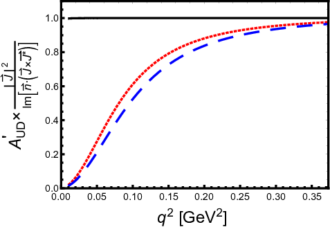
Figure 4: Results for up-down asymmetry AU​D′A_{UD}^{\prime} (in unit of Im⁡[n→⋅(J→×J→∗)]/|J→|2{\rm Im}[\vec{n}\cdot(\vec{J}\times\vec{J}^{*})]/|\vec{J}|^{2}) in D→K1(→Kππ)ℓ+νℓD\to K_{1}(\to K\pi\pi)\ell^{+}\nu_{\ell}. The solid curve corresponds to the electron final state, in which the lepton mass is negligible and the result is very close to unity. The dashed and dotted results correspond to the muon mode with the mixing angle ΘK=60∘\Theta_{K}=60^{\circ} and ΘK=30∘\Theta_{K}=30^{\circ}, respectively. The nonzero mass of μ\mu provides sizable corrections as shown in Eq. (29).

Results for up-down asymmetry AU​D′A_{UD}^{\prime} (in unit of Im⁡[n→⋅(J→×J→∗)]/|J→|2{\rm Im}[\vec{n}\cdot(\vec{J}\times\vec{J}^{*})]/|\vec{J}|^{2}) in D→K1​(1270)​ℓ+​νℓD\to K_{1}(1270)\ell^{+}\nu_{\ell} are shown in Fig. 4. The solid curve corresponds to the electron final state, in which the lepton mass is negligible and the result is very close to unity. The dashed and dotted results correspond to the muon mode with the mixing angle ΘK=60∘\Theta_{K}=60^{\circ} and ΘK=30∘\Theta_{K}=30^{\circ}, respectively. From this figure, one can see that the nonzero mass of muon can give considerable corrections also shown in Eq. (29), but the results are less sensitive to the D→K1D\to K_{1} form factors.

Integrating over the q2q^{2}, we obtain the angular distributions of D→K1(→Kππ)ℓ+νℓD\to K_{1}(\to K\pi\pi)\ell^{+}\nu_{\ell} dataset as

d​ΓdcosθℓdcosθK=\displaystyle\frac{d\Gamma}{d\cos\theta_{\ell}d\cos\theta_{K}}= a1+a2[cos2θKcos2θℓ]+a3cosθℓ+a4cos2θKcosθℓ\displaystyle a_{1}+a_{2}[\cos^{2}\theta_{K}\cos^{2}\theta_{\ell}]+a_{3}\cos\theta_{\ell}+a_{4}\cos^{2}\theta_{K}\cos\theta_{\ell}
+\displaystyle+ a5cosθK+a6cosθKcos2θℓ+a7cosθKcosθℓ+a8cos2θK+a9cos2θℓ,\displaystyle a_{5}\cos\theta_{K}+a_{6}\cos\theta_{K}\cos^{2}\theta_{\ell}+a_{7}\cos\theta_{K}\cos\theta_{\ell}+a_{8}\cos^{2}\theta_{K}+a_{9}\cos^{2}\theta_{\ell}, (45)

with

ai=38​∫d​q2​GF2​Vc​s2​q2​λ⁡(mD2,mK12,q2)512​π3​mD3​(1−mℓ2/q2)2×di.\displaystyle a_{i}=\frac{3}{8}\int dq^{2}\frac{G^{2}_{F}V^{2}_{cs}q^{2}\sqrt{\lambda(m^{2}_{D},m^{2}_{K_{1}},q^{2})}}{512\pi^{3}m_{D}^{3}}(1-m_{\ell}^{2}/q^{2})^{2}\times d_{i}. (46)

As an illustration, we use a standalone fast simulation software RapidSim Cowan:2016tnm with the LHCb geometrical acceptance to generate MC samples. D0→K1​(1270)−​μ+​νμD^{0}\to K_{1}(1270)^{-}\mu^{+}\nu_{\mu} decays are described by EVTGEN Lange:2001uf with the ISGW2 model Scora:1995ty. In the simulation, we have generated about 1.7×1061.7\times 10^{6} events with three decay modes for K1​(1270)−K_{1}(1270)^{-}: about 10610^{6} events for D→K1(→ρ(→ππ)K)μ+νμD\to K_{1}(\to\rho(\to\pi\pi)K)\mu^{+}\nu_{\mu}, 0.5×1060.5\times 10^{6} events for D→K1(→K∗(892)(→Kπ)π)μ+νμD\to K_{1}(\to K^{*}(892)(\to K\pi)\pi)\mu^{+}\nu_{\mu} and 0.2×1060.2\times 10^{6} for D→K1(→Kππ)μ+νμD\to K_{1}(\to K\pi\pi)\mu^{+}\nu_{\mu} in which the K1K_{1} decay is produced according to phase space. A comparison of fitting these MC samples using the formula 45 and the one from previous work Wang:2019wee is given in Fig. 5, and a detailed analysis of each component is given in Fig. 6. Through these figures, one can see that our simulated angular distributions can not be well described by the angular distribution in the previous work Wang:2019wee. With the inclusion of the muon mass, the agreement between theoretical description and angular distributions of MC events is greatly improved.

Refer to caption
Figure 5: Fit to 1.7×1061.7\times 10^{6} MC events with 3 components using two models: mlm_{l}=0(Red) and ml≠0m_{l}\neq 0 (Blue)
Refer to caption
Refer to caption
Refer to caption
Figure 6: Fit to 0.2×1060.2\times 10^{6} D→K1(→Kππ)μ+νμD\to K_{1}(\to K\pi\pi)\mu^{+}\nu_{\mu} (upper), 0.5×1060.5\times 10^{6} D→K1(→K∗(892)(→Kπ)π)μ+νμD\to K_{1}(\to K^{*}(892)(\to K\pi)\pi)\mu^{+}\nu_{\mu} (middle) and 10610^{6} D→K1(→ρ(→ππ)K)μ+νμD\to K_{1}(\to\rho(\to\pi\pi)K)\mu^{+}\nu_{\mu}(lower) MC events using two models: mlm_{l}=0(Red) and ml≠0m_{l}\neq 0 (Blue)

IV Summary

Weak decays of heavy quarks have played an important role in testing standard model and probing new physics beyond. Recent studies of flavor-changing neutral current process has revealed some hints for potential NP effects (see for instance Ref. Aaij:2021vac), but a conclusive result is far from well-established, and requests more dedicated theoretical and experimental studies in future Cerri:2018ypt. At the same time, the photon helicity in b→s​γb\to s\gamma might render very competitive potentials for new physics Aaij:2020umj.

Based on a previous proposal to pin down hadronic uncertainties in B→K1​γB\to K_{1}\gamma Wang:2019wee, we have in this work systematically derived differential decay widths and angular distributions for the decay cascade D→K1​(1270,1400)​ℓ+​νℓ→(K​π​π)​ℓ+​νℓ​(ℓ=e,μ)D\to K_{1}(1270,1400)\ell^{+}\nu_{\ell}\to(K\pi\pi)\ell^{+}\nu_{\ell}(\ell=e,\mu). In the derivation, the mass of electron/muon is explicitly included. Using the D→K1D\to K_{1} form factors from light-front quark model, we have calculated partial decay widths and branching fractions for D0→K1−​ℓ+​νℓD^{0}\to K_{1}^{-}\ell^{+}\nu_{\ell} and D+→K10​ℓ+​νℓD^{+}\to K_{1}^{0}\ell^{+}\nu_{\ell}, but pointed out that these theoretical results for ℬ⁡(D→K1​e+​νe){\cal B}(D\to K_{1}e^{+}\nu_{e}) are about a factor 1.5 higher than recent BESIII measurements.

With the angular coefficients, we have demonstrated that the measurement of up-down asymmetry in D→K1​e+​νe→(K​π​π)​e+​νeD\to K_{1}e^{+}\nu_{e}\to(K\pi\pi)e^{+}\nu_{e} and the angular distribution in D→K1​ℓ+​νℓ→(K​π​π)​ℓ+​νℓD\to K_{1}\ell^{+}\nu_{\ell}\to(K\pi\pi)\ell^{+}\nu_{\ell} can help to pin down hadronic uncertainties in B→K1(→Kππ)γB\to K_{1}(\to K\pi\pi)\gamma. Based on the Monte-Carlo simulation, we have found that after including the muon mass, the angular distributions can be well described by the theoretical framework.

Acknowledgement

W.W. thanks Fu-Sheng Yu and Zhen-Xing Zhao for valuable discussions and the collaboration at the early stage of this work. The authors are grateful to Fei Huang, Xian-Wei Kang, Xiao-Rui Lyu, Wen-Bin Qian, Yang-Heng Zheng for useful discussions. This work is supported in part by Natural Science Foundation of China under grant No.11735010, U1932108, U2032102, 12061131006, and 12061141006, by Natural Science Foundation of Shanghai under grant No. 15DZ2272100.

References

  • (1) D. Atwood, M. Gronau and A. Soni, Phys. Rev. Lett. 79, 185-188 (1997) doi:10.1103/PhysRevLett.79.185 [arXiv:hep-ph/9704272 [hep-ph]].
  • (2) D. Becirevic, E. Kou, A. Le Yaouanc and A. Tayduganov, JHEP 08, 090 (2012) doi:10.1007/JHEP08(2012)090 [arXiv:1206.1502 [hep-ph]].
  • (3) A. Paul and D. M. Straub, JHEP 04, 027 (2017) doi:10.1007/JHEP04(2017)027 [arXiv:1608.02556 [hep-ph]].
  • (4) E. Kou, C. D. Lü and F. S. Yu, JHEP 12, 102 (2013) doi:10.1007/JHEP12(2013)102 [arXiv:1305.3173 [hep-ph]].
  • (5) N. Haba, H. Ishida, T. Nakaya, Y. Shimizu and R. Takahashi, JHEP 03, 160 (2015) doi:10.1007/JHEP03(2015)160 [arXiv:1501.00668 [hep-ph]].
  • (6) B. Aubert et al. [BaBar], Phys. Rev. D 77, 051103 (2008) doi:10.1103/PhysRevD.77.051103 [arXiv:0711.4889 [hep-ex]].
  • (7) J. P. Lees et al. [BaBar], Phys. Rev. Lett. 109, 191801 (2012) doi:10.1103/PhysRevLett.109.191801 [arXiv:1207.2690 [hep-ex]].
  • (8) J. P. Lees et al. [BaBar], Phys. Rev. D 86, 052012 (2012) doi:10.1103/PhysRevD.86.052012 [arXiv:1207.2520 [hep-ex]].
  • (9) T. Saito et al. [Belle], Phys. Rev. D 91, no.5, 052004 (2015) doi:10.1103/PhysRevD.91.052004 [arXiv:1411.7198 [hep-ex]].
  • (10) Y. Ushiroda et al. [Belle], Phys. Rev. D 74, 111104 (2006) doi:10.1103/PhysRevD.74.111104 [arXiv:hep-ex/0608017 [hep-ex]].
  • (11) B. Aubert et al. [BaBar], Phys. Rev. D 78, 071102 (2008) doi:10.1103/PhysRevD.78.071102 [arXiv:0807.3103 [hep-ex]].
  • (12) R. Aaij et al. [LHCb], Phys. Rev. Lett. 123, no.8, 081802 (2019) doi:10.1103/PhysRevLett.123.081802 [arXiv:1905.06284 [hep-ex]].
  • (13) S. Akar, E. Ben-Haim, J. Hebinger, E. Kou and F. S. Yu, JHEP 09, 034 (2019) doi:10.1007/JHEP09(2019)034 [arXiv:1802.09433 [hep-ph]].
  • (14) Y. Grossman and D. Pirjol, JHEP 06, 029 (2000) doi:10.1088/1126-6708/2000/06/029 [arXiv:hep-ph/0005069 [hep-ph]].
  • (15) R. Aaij et al. [LHCb], JHEP 12, 081 (2020) doi:10.1007/JHEP12(2020)081 [arXiv:2010.06011 [hep-ex]].
  • (16) S. de Boer and G. Hiller, Eur. Phys. J. C 78, no.3, 188 (2018) doi:10.1140/epjc/s10052-018-5682-7 [arXiv:1802.02769 [hep-ph]].
  • (17) M. Gronau, Y. Grossman, D. Pirjol and A. Ryd, Phys. Rev. Lett. 88, 051802 (2002) doi:10.1103/PhysRevLett.88.051802 [arXiv:hep-ph/0107254 [hep-ph]].
  • (18) M. Gronau and D. Pirjol, Phys. Rev. D 66, 054008 (2002) doi:10.1103/PhysRevD.66.054008 [arXiv:hep-ph/0205065 [hep-ph]].
  • (19) E. Kou, A. Le Yaouanc and A. Tayduganov, Phys. Rev. D 83, 094007 (2011) doi:10.1103/PhysRevD.83.094007 [arXiv:1011.6593 [hep-ph]].
  • (20) R. Aaij et al. [LHCb], Phys. Rev. Lett. 112, no.16, 161801 (2014) doi:10.1103/PhysRevLett.112.161801 [arXiv:1402.6852 [hep-ex]].
  • (21) A. Tayduganov, E. Kou and A. Le Yaouanc, Phys. Rev. D 85, 074011 (2012) doi:10.1103/PhysRevD.85.074011 [arXiv:1111.6307 [hep-ph]].
  • (22) M. Gronau and D. Pirjol, Phys. Rev. D 96, no.1, 013002 (2017) doi:10.1103/PhysRevD.96.013002 [arXiv:1704.05280 [hep-ph]].
  • (23) W. Wang, F. S. Yu and Z. X. Zhao, Phys. Rev. Lett. 125, no.5, 051802 (2020) doi:10.1103/PhysRevLett.125.051802 [arXiv:1909.13083 [hep-ph]].
  • (24) R. H. Li, C. D. Lu and W. Wang, Phys. Rev. D 79, 034014 (2009) doi:10.1103/PhysRevD.79.034014 [arXiv:0901.0307 [hep-ph]].
  • (25) W. Wang and Z. X. Zhao, Eur. Phys. J. C 76, no.2, 59 (2016) doi:10.1140/epjc/s10052-016-3900-8 [arXiv:1511.06998 [hep-ph]].
  • (26) H. Y. Cheng, C. K. Chua and C. W. Hwang, Phys. Rev. D 69, 074025 (2004) doi:10.1103/PhysRevD.69.074025 [arXiv:hep-ph/0310359 [hep-ph]].
  • (27) P. A. Zyla et al. [Particle Data Group], PTEP 2020, no.8, 083C01 (2020) doi:10.1093/ptep/ptaa104
  • (28) K. C. Yang, Nucl. Phys. B 776, 187-257 (2007) doi:10.1016/j.nuclphysb.2007.03.046 [arXiv:0705.0692 [hep-ph]].
  • (29) K. Abe et al. [Belle], [arXiv:hep-ex/0408138 [hep-ex]].
  • (30) K. Hayasaka, Z. Huang and E. Kou, [arXiv:2102.00752 [hep-ph]].
  • (31) R. C. Verma, J. Phys. G 39, 025005 (2012) doi:10.1088/0954-3899/39/2/025005 [arXiv:1103.2973 [hep-ph]].
  • (32) H. Y. Cheng and X. W. Kang, Eur. Phys. J. C 77, no.9, 587 (2017) [erratum: Eur. Phys. J. C 77, no.12, 863 (2017)] doi:10.1140/epjc/s10052-017-5170-5 [arXiv:1707.02851 [hep-ph]].
  • (33) Q. Chang, X. L. Wang and L. T. Wang, Chin. Phys. C 44, no.8, 083105 (2020) doi:10.1088/1674-1137/44/8/083105 [arXiv:2003.10833 [hep-ph]].
  • (34) S. Momeni and R. Khosravi, J. Phys. G 46, no.10, 105006 (2019) doi:10.1088/1361-6471/ab35d0 [arXiv:1903.00860 [hep-ph]].
  • (35) R. Khosravi, K. Azizi and N. Ghahramany, Phys. Rev. D 79, 036004 (2009) doi:10.1103/PhysRevD.79.036004 [arXiv:0812.1352 [hep-ph]].
  • (36) S. Momeni, Eur. Phys. J. C 80, no.6, 553 (2020) doi:10.1140/epjc/s10052-020-8084-6 [arXiv:2004.02522 [hep-ph]].
  • (37) M. Ablikim et al. [BESIII], Phys. Rev. Lett. 123, no.23, 231801 (2019) doi:10.1103/PhysRevLett.123.231801 [arXiv:1907.11370 [hep-ex]].
  • (38) M. Ablikim et al. [BESIII], [arXiv:2102.10850 [hep-ex]].
  • (39) G. A. Cowan, D. C. Craik and M. D. Needham, Comput. Phys. Commun. 214, 239-246 (2017) doi:10.1016/j.cpc.2017.01.029 [arXiv:1612.07489 [hep-ex]].
  • (40) D. J. Lange, Nucl. Instrum. Meth. A 462, 152-155 (2001) doi:10.1016/S0168-9002(01)00089-4
  • (41) D. Scora and N. Isgur, Phys. Rev. D 52, 2783-2812 (1995) doi:10.1103/PhysRevD.52.2783 [arXiv:hep-ph/9503486 [hep-ph]].
  • (42) R. Aaij et al. [LHCb], [arXiv:2103.11769 [hep-ex]].
  • (43) A. Cerri, V. V. Gligorov, S. Malvezzi, J. Martin Camalich, J. Zupan, S. Akar, J. Alimena, B. C. Allanach, W. Altmannshofer and L. Anderlini, et al. CERN Yellow Rep. Monogr. 7, 867-1158 (2019) doi:10.23731/CYRM-2019-007.867 [arXiv:1812.07638 [hep-ph]].