Estimating customer delay and tardiness sensitivity from periodic queue length observations
Abstract
A single server commences its service at time zero every day. A random number of customers decide when to arrive to the system so as to minimize the waiting time and tardiness costs. The costs are proportional to the waiting time and the tardiness with rates and , respectively. Each customer’s optimal arrival time depends on the others’ decisions, thus the resulting strategy is a Nash equilibrium. This work considers the estimation of the ratio from queue length data observed daily at discrete time points, given that customers use a Nash equilibrium arrival strategy. A method of moments estimator is constructed from the equilibrium conditions. Remarkably, the method does not require estimation of the Nash equilibrium arrival strategy itself, or even an accurate estimate of its support. The estimator is strongly consistent and the estimation error is asymptotically normal. Moreover, the asymptotic variance of the estimation error as a function of the queue length covariance matrix (at sampling times) is derived. The estimator performance is demonstrated through simulations, and is shown to be robust to the number of sampling instants each day.
Keywords— Strategic arrival times to a queue; Parameter Estimation; Transient queueing; Tardiness
1 Introduction
When the quality of a product or a service deteriorates with time, an important consideration of customers is to avoid service delay. It occurs quite often that customers arrive at a supermarket earlier in order to obtain fresh products. An expensive managing warehouse always expects items to be picked up as soon as possible (see Elsayed, Lee, Kim, and Scherer 1993). The earlier a customer gets in a concert, the better seat she can take (see Jain, Juneja and Shimkin 2011). In these cases, tardiness, measured from the opening time to the service commencement time of a customer, needs to be incorporated as a measure of the cost.
Customers typically try to avoid congestion. In particular, besides not being late, a customer hopes to wait for as little time as possible. Assume that the cost is linear in time with rates and for the waiting and tardiness, respectively. Then in deciding when to arrive, a customer needs to balance between arriving earlier and waiting less, and the optimal decision is affected by the ratio . While the literature on strategic arrivals to queueing systems with tardiness costs provides considerable methods to describe and obtain the Nash equilibrium (e.g., Haviv 2013; Juneja and Shimkin 2013), it assumes that the system parameters are known beforehand. The problem of estimation concerning the cost rates has received little attention. In this paper, we estimate the ratio from the queue length information.
We consider a single server queueing system with a first-come first-served (FCFS) discipline, which commences its service at time zero every day. The service time is exponentially distributed with rate . The system can have a pre-imposed closing time or not. Let be the service closing time, then the system serves all the customers who arrive prior to time (inclusive). When , the system closes after it serves all arriving customers. Every day, a Poisson number, with mean , of customers each decide when to arrive to this system, so as to minimize their expected waiting and tardiness cost. When , as is finite, the system still serves all the arriving customers in a finite time. Thus, we still call it a day.
The FCFS queueing discipline implies that the expected cost of a customer depends on the number of customers who arrived before her, which is affected by the other customers’ decisions. As a consequence, the best response of each customer is a function of the other customers’ actions. It is thus appropriate to model this interaction as a non-cooperative game with the solution concept of a Nash equilibrium strategy. We focus on the symmetric mixed Nash equilibrium, which dictates that all customers have the same strategy, which is a probability distribution on .
Our general framework allows for two model variations in which customers queueing before time zero is possible, or not. As in Haviv 2013, we refer to these variations as with early birds and without early birds. In the with early birds case, customers arriving before time zero are served according to a FCFS discipline. In the without early birds case, customers who arrive before time zero are served in a random order. Hence, arriving before time zero does not bring extra benefit but incurs additional waiting costs, compared with arriving at time zero. So in the Nash equilibrium, customers do not arrive at any time .
We assume that customers arrive according to the Nash equilibrium every day, and their decisions are independent on different days. The values of and are known to the customers but not to the system manager. To estimate the ratio , the system manager can sample the queue length at a collection of time instants every day. Note that although the observations from different days are independent, the observations from different time points in one day are not. We assume that the sampling instants are the same on all days. An estimator for is then derived by using the property that in Nash equilibrium the expected cost is equal at any time with a positive arrival rate.
1.1 Literature review
Haviv 2013 derived the Nash equilibrium arrival distribution for the system that this work focuses on. The study of the strategic arrival time choice in queueing models goes back to Glazer and Hassin 1983, which studied a single server system with a Poisson number of customers that decide when to arrive with the goal of minimizing their expected waiting time. The Nash equilibrium arrival distribution is characterized as a solution of a system of functional differential equations that satisfy a condition of constant cost throughout the arrival support. Jain, Juneja and Shimkin 2011 considered a concert queueing game with waiting and tardiness costs using a fluid approximation which enables closed form derivation of the equilibrium arrival distribution. Juneja and Shimkin 2013 studied the stochastic version of the concert queueing game with a general number of customers, and characterized the symmetric Nash equilibrium arrival distribution in terms of a set of differential equations, and argued that it is absolutely continuous. In particular, they proved that a unique equilibrium exists and it is symmetric. Haviv and Ravner 2015 studied strategic timing of arrivals to a multi-server loss system, where customers tried to maximize their probability of receiving the service. Comprehensive reviews and summaries of this line of research can be found in Haviv and Ravner 2021 and Hassin 2016.
Most of the literature that deals with queueing process estimation concerns the arrival and service rates, and describes methods that require continuous observation over an interval of time. To cite but a few, see for example Bhat and Rao 1987, Armero 1994, Armero and Armero 1994, Basawa and Prabhu 1988, Bingham and Pitts 1999. See Asanjarani, Nazarathy, and Taylor 2021 for a comprehensive survey of parameter estimation in queues. In Inoue, Ravner, and Mandjes 2020, the authors considered a system with strategic customers who can choose to balk after being aware of information about the delay, and estimated the patience distribution and the corresponding potential arrival rate. Robinson and Chen 2011 estimated the relative perceived value of patients waiting time, which is a ratio of the cost of the customers’ waiting time to the cost of the server’s idle time. Their method relies on constructing an estimation equation from the optimality condition of the stationary expected cost of the system. However, as opposed to our setting, customers are not strategic and the underlying distribution of the queueing process is known.
1.2 Outline of the methods and contribution
Before presenting the estimation method we need to first look into the Nash equilibrium dynamics. A symmetric Nash equilibrium is an arrival strategy that it is optimal for any customer if it is also used by all others. We denote the Nash equilibrium distribution by , the corresponding probability density by . The full details of deriving the symmetric equilibrium can be found in Haviv 2013. We only consider the non-trivial case where is large enough such that there are customers willing to arrive after time . For the sake of brevity we primarily focus on the no early bird variation where there are no arrivals before time and no service closing time (i.e., ). However, in Section 6, we show that with modifications the method can be applied to the other model variations as well. Moreover, the methodology in this work can be extended to other queueing systems with strategic choice of arrival times.
Let be the cost and waiting time, respectively, for a customer who arrives at time , then
If all other customers use , her expected cost is
| (1.1) |
In equilibrium for any in the support of the arrival distribution, where is a constant, and for any not in the support. This type of equilibrium is also known as a Wardrop equilibrium (Wardrop 1952).
The first step towards estimating is to estimate the expected waiting time at sampling instants within the support of the arrival distribution, which is a linear function of the expected number of customers in the queue due to the exponential service assumption and the FCFS discipline. Estimation of the support will be explained in detail in Section 3.2. Suppose are in the support with , then we can express the expected costs and in terms of , and the expected waiting times of customers arriving at the two times, using Equation (1.1). By setting we will show that can be expressed in terms of the expected number of customers at the two time instants: As service times are exponential,
where is the queue length process. Hence, by (1.1),
This yields a moment estimation equation for any pair of sampling instants . If the queue length is sampled at a collection of times, then a refined estimator is given by taking average of the estimators corresponding to all pairs.
We demonstrate the performance of our estimator through asymptotic analysis and simulation studies. Specifically, we prove strong consistency and asymptotic normality of the resulting estimator. The proofs rely on establishing the law of large numbers and central limit theorems for the expected queue length estimators and then applying the continuous mapping theorem. We further derive an expression for the asymptotic variance of the estimation error as a function of the covariance matrix of the queue lengths at sampling times. We also explain how the asymptotic variance can be numerically approximated. Remarkably, the asymptotic performance is guaranteed even if the queue length is only sampled three times every day (as long as the sampling times are in the positive support of the equilibrium arrival distribution). However, sampling at multiple instants and spacing these instants far apart can improve the statistical efficiency in terms of the asymptotic variance. This is illustrated through simulation experiments in Section 3. The main finding of the simulation study is that only a small number of sampling instants are required to reduce the variance of the estimation error. In other words, there is almost no difference between continuous observation of the queue length and sampling it at a small number of time instants.
Our study constructs an estimator of utility parameters of strategic customers by taking advantage of the queueing dynamics brought corresponding to a Nash equilibrium. Moreover, to the best of the authors’ knowledge this is the only work to do so for a transient queueing setting. Second, the estimation methodology is applicable for a number of systems with strategic customers whose choice is of the Wardrop equilibria type. The setting that customers are strategic is essential in this work, since our method makes use of the properties of expected cost faced by customers arriving according to the Nash equilibrium distribution. Third, the estimator we propose needs substantially less information than standard queueing inference techniques (see Asanjarani, Nazarathy, and Taylor 2021). Namely, it does not require continuous observations, or an accurate estimate of the support of the equilibrium arrival distribution. In fact, with only two points in the support, we are able to estimate the ratio . We explain how to choose the two points in detail in Section 3. Moreover, as explained above, simulation analysis suggests that the estimator is robust to the number of sampling instants each day.
The remainder of the paper is organised as follows. In Section 2 we explain the Nash equilibrium arrival distribution and how to numerically calculate it. In Section 3 the estimator for is presented for the case where there are no arrivals before time . Section 4 presents the asymptotic analysis of the estimator. In Section 5 we provide several numerical examples to demonstrate the effect of the number of the observation days and the sampling instants on the estimator. In Section 6 we modify the estimator for the cases where there are arrivals before time or a service closing time. Section 6 further discusses the potential to extend our estimation method to more elaborate systems with strategic arrival time choice.
2 Preliminaries
In this section, we summarize the results of Haviv 2013 and Juneja and Shimkin 2013 that characterize the Nash equilibrium arrival distribution and the associated expected costs. In Appendix A we illustrate how to approximate the equilibrium distribution and the expected cost for the case where there are no arrivals before time , via the finite difference method.
Let be the queue length at time , and for . In the case where there are no arrivals before time , if there is no closing time, there exist such that the equilibrium arrival distribution is given by
| (2.1) | ||||
| (2.2) |
That is, there is an atom of size at time zero, no arrivals during the interval , a positive density along , and for .
Note that if there is a service closing time , then Nash equilibrium has three cases (Haviv 2013, Theorem 3.2). If , where is determined by (2.1) and (2.2), then the Nash equilibrium is to arrive at time zero with probability . We do not consider this case in our paper. If , the equilibrium arrival distribution is similar to the case with no closing time, but the arrival distribution support is and . In particular, the values of , , and satisfy
| (2.3) | ||||
| (2.4) |
If , the equilibrium arrival distribution is the same as the case with no service closing time.
In the case where arrivals before time zero are allowed and there is no closing time, there exist such that the equilibrium arrival distribution has
| (2.5) | ||||
| (2.6) |
There is a constant density along , and positive density along . Note that in (2.1), (2.3), and (2.5) depends on the corresponding Nash equilibrium arrival distribution. It can be seen from Equation (2.1)-(2.6) that the distribution is determined by the ratio , not the specific values of and . For all of the above cases Juneja and Shimkin 2013 proved that the equilibrium solution is unique and absolutely continuous (excluding a possible discontinuity at zero).
In the following analysis, we mainly focus on the case where there are no arrivals before time and no service closing time. Later, in Section 6, we show that the estimator we propose can be easily adapted for other cases. Let be as defined in Equation (1.1), then a Nash equilibrium satisfies
| (2.7) |
and
| (2.8) |
This is because a customer only randomize arrival time points if they result in the same cost. Secondly, the expected cost of a customer arriving at any point outside cannot be lower. Otherwise, a customer would be better off by deviating to such an arrival time.
The expected cost for the case without early birds can then be written as
| (2.9) |
Observe that at time zero there is a positive mass of customers arriving together that are served in random order. Hence, a customer arriving at time zero will on average have to wait for half of the other customers that also arrived with her. To numerically obtain the equilibrium distribution and the associated cost, we employ a finite difference approximation. In particular, we assume that customers can choose to arrive at a time on a discrete grid for a small . Appendix A provides details of this approximation.
3 Estimation of
From now on we assume that customers arrive according to the symmetric Nash equilibrium arrival distribution . We denote , while keeping in mind that all expectations are still with respect to the probability measure imposed by the arrival distribution . Assume that the system manager knows the value of , but not . It follows from Equation (2.1) that is determined by , , and . Note that if is unknown it can be easily estimated, for example by observing a collection of service times. Moreover, the following estimation method does not require knowledge of . Thus, the distribution of the queue length process is a function of via . The question is how to construct an estimator for from observations of the queue length. By the definition of the Nash equilibrium, when others arrive according to , each customer is indifferent between arriving at any . Hence, Equations (2.7) and (2.9) imply that
| (3.1) |
Then we can write down the expression for the expected cost of any two points in , and derive in terms of the expected queue length at these two points. For any , we have
| (3.2) | ||||
and for ,
| (3.3) | ||||
We conclude that can be expressed as a function of the expected queue length at any two observation instants in . This enables the construction of a method of moments type estimator for from any two observation times. Multiple estimators are obtained when the queue length is observed at more than two time instants, and in that case the mean of all estimators can be taken. In particular, the queue length is inspected at the collection of times , where . The sampling process is repeated for days, with the same sampling times every day. Towards the construction of the estimator we first detail the necessary preliminary steps: estimation of the expected queue lengths and of the support of the equilibrium arrival distribution, i.e., the values and .
3.1 Estimation of the expected queue lengths
Given the equilibrium arrival distribution , we can calculate the expected queue length . Algorithm 1 in the appendix outlines how this is done using the discrete approximation scheme for the computation of . Figure 1 depicts , two observations can be made. Firstly, is a linear function on , whose slope is , this can also be derived from Equation (3.3). Second, if we extend the line to , then the point intersecting with is , which can also be inferred from Equation (3.2).


Equation (3.2) and (3.3) imply that two observation points in the support each day are enough to estimate . However, observe that to use (3.2) or (3.3), we first need to estimate . To achieve this we need more than two observations as will be shown in Section 3.2.
Suppose we choose a collection of time instants to observe the queue length every day. Let and be the number of observation days and the number of sampling instants every day, respectively. For , we denote by and the th observation time point and the queue length at that point on the th day. We assume that the observations are obtained at the same time instants every day, so we drop the index on and denote the samples on the th day as . Note that sampling at exactly the same time instants ensures that the observed daily queue length vectors are independent and identically distributed. It follows from our assumption of statistical independence between days that are from independent realisations of the process. Since are independent and identically distributed as , the expected queue length can be estimated by the sample mean
at the th sampling time instant.
Figure 2 depicts for three simulations with and , compared to the expected queue length . Note that both the simulation and the expected queue length first require numerical evaluation of using Algorithm 2. Observe that the queue length estimators yield an unbiased, but noisy, representation of the actual expected queue length process. It is therefore important to use multiple time instants throughout the day in order to reduce the variance of the estimation error. For illustration purposes a very fine grid is used (), however we will later show that a very coarse grid is actually sufficient for achieving very good estimation accuracy. The intuition here is that the queue lengths at very close time instants are highly correlated and thus it is more informative to sample the process with a bigger space between observation instants.

Remark 1.
We focus on the model with no service closing time, i.e., . Of course, for practical purposes we must impose a simulation stopping time, denoted by . Intuitively, for a good choice there should be a non-empty time interval that does not have any arrival for any of the simulation iterations. Indeed, if is greater than , then the strategic behavior of the customers is not affected by the choice of . We set for all simulation analysis in the remainder of the paper, that is, is the grid we run our simulation on. For the parameter configurations and we used , since we know from the numerical evaluation of that for these configurations. In practice, choosing the simulation time is a trial-and-error process. Note that even if , the estimator of is biased, but the estimation of is not (as long as there is a non-empty time interval with arrivals).
3.2 Estimation of the support
To estimate and we must identify the first and last time instants in such that the queue length increases. By noticing that must include these times, we estimate the support boundaries by
| (3.4) | ||||
| (3.5) |
Denote the boundaries of the intersection of the support and the discrete observation grid by
| (3.6) | ||||
| (3.7) |
and observe that . Due to the discrete observation scheme, one cannot accurately estimate and . However, we can estimate and by and , respectively. Figure 3 describes some examples of and with plotted as well, where the shaded interval is . In Figure 3 (a), the observation instants includes both and , but this is only possible for carefully chosen parameters such that the boundaries of the discrete grid coincide with those of the support. In this case, and . In general does not include or , as in Figure 3 (b) (c) (d). In any case, it follows from (3.4) and (3.5) that
Recall that the reason for estimating the support is to be able to select time points inside and use the average number of customers at these time points to estimate . Even if the estimation for the support is biased, the estimation for is not affected by the bias as long as the chosen pair is inside , which always holds since .
3.3 Estimation of using a reference point
Let , where depends on . The interpretation of is the observation time slots in the estimated support . Applying (3.2) and (3.3) yields an estimator for ,
| (3.8) |
Note that symmetry implies . Further observe that for a finite sample there is a positive probability that some of the estimators fall outside of the interval . In the sequel we verify that the probability of such an event vanishes as the sample size grows.
To evaluate the performance of this estimator with respect to a choice of a reference point, we consider two parameter configurations and simulated data. The estimators for the boundary indices and are obtained using Equations (3.4) and (3.5). We then selected a time point as a reference point. For each , the estimator is calculated. The two examples of the sequences of estimators for where and , under different parameter settings are depicted in Figure 4. In Figure 4 (a), , the estimates and are and , respectively. In Figure 4 (b), , the estimates and are and , respectively. The true value is plotted by the dotted line, and the at is . It can be observed from both plots that the closer the two points are, the more biased the estimation is. The explanation is that the dependence between the queue lengths at two time slots increases when the distance between them decreases. In Section 4, we will see the estimator variance increases in quadratic rate with the distance.


Remark 2.
It follows from Equation (2.1) and that can also be expressed as
| (3.9) |
This means if we can estimate by , we can estimate by counting how many empty queues there are at and dividing it by the total sample size , thus yielding an estimator for . However, this requires an accurate estimate of first, which requires both a large such that includes a point that is very close to it, and a large sample size . Moreover, for any the estimator for is biased so it may not be possible to obtain a consistent estimator. Also, in the model with service closing time, which we discuss in Section 6, there does not necessarily exist a time that satisfies , thus there is no expression equivalent to (3.9).
3.4 The mean estimator


With the aforementioned reasoning in mind, it is better to choose two observation points that are far away from each other. For any , let and we compute for . The results for the examples considered in the prequel are depicted in Figure 5. The true value was plotted by the dotted line, and the at is . It is observed from the plots that is generally better than for a fixed reference point . This is specially noticeable for near . Denote the cardinality of by . When , we propose an estimator
| (3.10) |
by taking the mean of the estimates calculated by every pair in .
An overview of the observation and the estimation process is depicted in Figure 6. The manager uses her observations and the known value of to estimate . First the expected queue lengths are estimated from independent realizations of the queue. Next the interval of continuous arrivals is estimated by considering the time points closest to the boundaries on the discrete observation grid . Note that although the observations from different days are independent, the observations at different times for a single day are not, hence there is a need to carefully select the pairing of observation instants in the construction of the sequence of estimators for . To this end a heuristic rule of choosing the farthest away observation (in terms of time) is applied to every sampling time instant. The intuitive explanation for this rule is that the correlation between queue lengths at different sampling times decreases the further apart they are chosen. This intuition is verified by the examples presented above and simulation experiments in Section 5. Finally, the estimator in (3.10) is given by taking the mean of the sequence of estimators obtained by the optimal pairing rule.
4 Asymptotic analysis
We first state the main results of this section with the proofs detailed in the following subsections. In the following, denotes a normally distributed random variable with mean vector and covariance matrix . An estimator is said to be strongly consistent if as the number of observation days increases, the resulting sequence of estimates converges almost surely to the true value. Theorem 1 proves the strong consistency of our estimator . We establish the asymptotic normality of our estimator , and prove in Theorem 2 that as , the estimation error scaled by converges to a zero-mean normal random variable, whose variance can be numerically approximated. We explain in detail how the variance is calculated in Section 4.3. The proofs of Theorem 1 and 2 are provided in Section 4.1 and Section 4.2, respectively.
We assume the sampling points do not include time in this section. The analysis is similar if is included.
Theorem 1.
As , .
Theorem 2.
For , let , . Let and be the variance and covariance, for any . As ,
4.1 Strong consistency
The proof of Theorem 1 requires finite first and second moments of the queue length . The total number of customers in the system is bounded by a Poisson distributed random variables with mean , so as long as , and .
Proof of Theorem 1. The first and second moments of are bounded, it follows from Kolmogorov strong law of large numbers (Loeve 1977, p251) that
Also, it follows from Equation (3.8) and (3.10) that both and are linear functions of , thus the continuous mapping theorem in van der Vaart 2000 implies
We have explained in Section 3.2 that the reason to estimate the support is to be able to choose at least two points inside it for the estimation, and our method assures that . Moreover, with a discrete observation scheme the best one can hope for is to estimate the points on the grid that are closest to the actual boundaries of the support, i.e., and defined in Equations (3.6) and (3.7), respectively. Although it is not essential to have accurate estimates of and , we prove in the following proposition that and converges to and , respectively. Proposition 3 is used in establishing the asymptotic distribution of the errors in the proof of Theorem 2.
Proposition 3.
If there are at least two observation points from that are inside the support of the arrival distribution, then as , .
Proof.
We label the observation times in a way such that for . For , is increasing, so . By definition, is greater than or equal to . We will show that the probability that there are no days with an increase in queue length between the observation instants and goes to zero. The queue length increases if there are more arrivals than departures in this period. If such an increase is observed on day , then for all . Given that there are arrivals after time in equilibrium, the probability that there is at least one arrival but no departures during is at least
As the observations of different days are independent, we have that
Therefore,
Similarly, we have
and
Moreover, convergence in probability of a monotone sequence implies the convergence with probability 1 (Kallenberg 1997, Lemma 3.2), so we conclude
∎
4.2 Asymptotic distribution of the estimation error
Proof of Theorem 2. By Proposition 3 we know that converges almost surely to a fixed collection of times in . That is, the vector
converges almost surely to the same limit as
Moreover, for any satisfies the Central Limit Theorem because it is an average of independent and identically distributed observations with a known covariance matrix. Hence, letting
we have
where the covariance matrix is given by
Next, by (3.10) the estimator can be written as the linear combination
where and are as defined in Theorem 2. Again, Proposition 3 implies converges almost surely to . Let , the delta method (van der Vaart 2000, Chapter 3) can be applied to conclude that
4.3 The variance computation
As , converges to a zero-mean normal random variable with variance
| (4.1) |
The variance can be approximated numerically using a discrete approximation, similar to the one used for computing the expected queue length process. Observe that the unknown components in (4.1) are and . Following the scheme of Section A, given , we can calculate the queue length dynamics for . With , we can compute both the first moment and the second moment of the queue length at by and , respectively. Then can be obtained by calculating .
The calculation of is a bit more involved. From its definition,
| (4.2) |
where the first term can be written as
| (4.3) |
The reason to write by its conditional probability is that the joint probability cannot be approximated directly. Note that for numerical purposes truncation of the sums is required. The conditional probability can be obtained by calculating , given and , which indicates that we need to calculate for until .
5 Simulation analysis
This section presents simulation analysis of the performance of the estimator. Let be the number of simulations, and denote by the estimate of the th simulation, for . We compare the estimates obtained with the same number of observation points but different sample sizes . We also compare the estimates with the same sample size but different number of observation points each day. We use Box-plots to represent estimates of the 1000 simulations. On each box, the central mark indicates the median, and the bottom and top edges of the box indicate the 25th and 75th percentiles, respectively. The whiskers extend to the most extreme data points not considered outliers, and the outliers are plotted individually using the ’+’ marker symbol. In our performance analysis, we compute the average of the estimates (AE) and the root-mean-square deviation (RMSD) between and its estimate, which are defined as
The main result of this section is that the estimator is robust to the number of observation points .
As in the previous section, the simulations rely on the approximation of using the discrete scheme described in Appendix A. Let denote the th slot on the discrete grid, so is the time of the th observation. E.g. means that for . The sample is with , that is, we always consider time as an observation point. We first run simulations with , yielding , and , for . The Box-plots of are presented in Figure 7, and the AE and RMSD of the estimates are presented in Table 5.1 for each . It can be observed that although the estimator quality in terms of the mean and variance decreases with , the mean does not differ too much, and it is close to the true .

| AE | ||||
| RMSD | ||||
We next investigate how the value of affects the estimates. We assume that the inter observation times, denoted by , are equidistant. That is, , and for any . Since we set the simulation time , . Note that when the value of or is small, it is possible that and cannot be estimated. Thus, we use to denote the number of simulations for which was successfully estimated in the simulations we tried. We present the results of 1000 simulations with for , and show the estimates in Figure 8 (a). Figure 8 (b) depicts the asymptotic distribution of derived in Theorem 2. It can be seen that the estimator is robust to the value of . The mean is very close to the true for all values of . The variance is larger when the number of observations points is small. However, we further observe that increasing from does not noticeably impact the variance of the estimation error. The characteristics of the simulations results are summarized in Table 5.2 and it can be observed that the RMSD is less than for , while it is slightly higher for . It is important to point out that Figure 8 (b) is not the output of simulations, but rather a direct computation of the asymptotic variance from Theorem 2. Thus, this step can be carried out when designing a sampling scheme in order to determine the number of sampling instants required for good accuracy in terms of asymptotic variance of the estimation errors.


| () | () | () | () | |
| AE | ||||
| RMSD | ||||



| 0.0896 (0.0214) | 0.0893 (0.0238) | 0.0886 (0.0265) | 0.0878 (0.0396) | |
| 0.0906 (0.0152) | 0.0905 (0.0167) | 0.0900 (0.0189) | 0.0892 (0.0289) | |
| 0.0909 (0.0065) | 0.0909 (0.0070) | 0.0908 (0.0076) | 0.0904 (0.0127) | |
| 0.0909 (0.0046) | 0.0910 (0.0049) | 0.0910 (0.0053) | 0.0909 (0.0093) | |
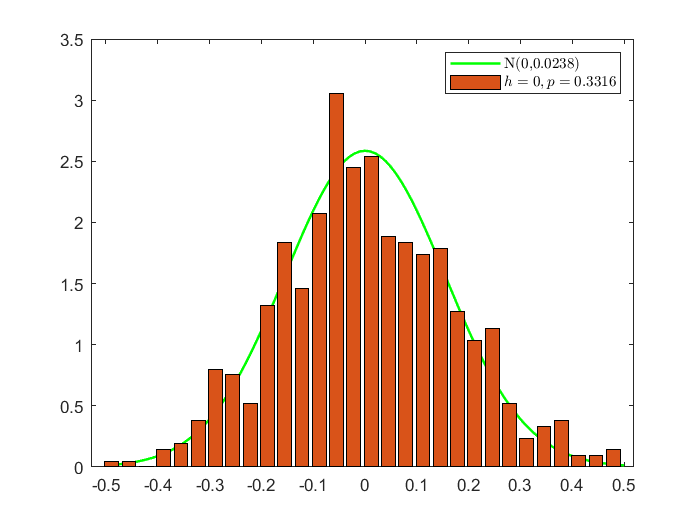
We applied a one-sample Kolmogorov-Smirnov test to check whether the estimates in Figure 8 (a) are from a given normal distribution. Specifically, we tested whether in the 1000 simulations come from a standard normal distribution, using function in Matlab. The function returns a test decision ( if the test rejects the null hypothesis at the 5% significance level, or otherwise) for the null hypothesis that the data comes from a standard normal distribution and the -value of the hypothesis test. Figure 9 depicts the normalized histograms of the 1000 simulations for . The asymptotic distribution of and the values of and are also denoted in the plot. The test results indicate that the normal approximation of Theorem 2 is very good for a sample size of .
The estimation accuracy is obviously a function of the number of days sampled, and as we saw in the previous section accurate estimation is guaranteed as . In some cases sampling the queue many times during the day may be costly and it is therefore of interest to explore how many sampling instances are required for a good estimator. To have an overview of estimates under different set, we calculate the estimates for , and summarize the results as AE (RMSD) in the first line, and in the second line in Table 5.3. The value of is also presented, and is by default, that is, if is not displayed, then all the 1000 simulations were successful. It can be seen that for , increases with with almost instants successful for . This further implies that for large enough sample sizes a good estimation can be obtained even for a small number of sampling times throughout the day. The estimator quality is relatively robust to the number of observations each day. However, when the sample size is small it is better to sample the queue more often during the day to ensure an accurate estimator is obtained. Also, when , the asymptotic normality of our estimator can already be observed when (as was also illustrated in Figure 8 (b)). The main conclusion from the simulation experiments is that a few observations of the queue length every day are sufficient for successful and accurate estimation of .
Finally, in practice, if sampling the queue is costly, we do not need to observe the queue length for times each day for every day. For example, we can observe it for several days with a large number of points, in order to estimate and first. Then, we only need to select more than one point (less than ) in to estimate . On the other hand, if the queue is only observable for a small number of days (i.e., small ), then it is better to sample more time instants within the day in order to increase the chance of successfully identifying times inside the support.
6 Extensions
The estimator in Section 3.4 can be easily modified to apply to the case with service closing time or the case where there are arrivals before time . For the model with service closing time, we only discuss the case where there are no arrivals before time . For other cases with service closing time, the analysis is similar.
If , the equilibrium arrival distribution is the same as the case service closing time, so the estimator is the same. When , although the equilibrium arrival distribution is different, the relationship in Equation (3.1) still holds, thus the estimator is exactly the same as proposed in Section 3. The only difference is that . With Algorithms 1 and 3 given in the appendix, we can calculate the equilibrium arrival distribution and the expected queue length . Both and are plotted in Figure 10 (a). It can be observed that the expected queue length is a straight line from to , and the slope can be used to estimate . The estimator in (3.10) works for the model with service closing time.


In the model where there are arrivals before time and no service closing time, the expected cost can be written as
| (6.1) |
Since the support of the arrival distribution is , and the expected cost faced by a customer if she arrives at any is the same, we have for ,
| (6.2) | ||||
for ,
| (6.3) | ||||
for ,
| (6.4) | ||||
| (6.5) |
Thus,
| (6.6) |
That is can be expressed as a function of the expected queue length at . Thus following the same estimation method as in Section 3, the estimator of can be constructed based on the sample mean of the observed queue lengths in an estimated support of . The equilibrium arrival distribution can be calculated using Algorithm 4. The expected queue length can then be calculated using 1. Both and are plotted in Figure 10 (b). It can be inferred from Equation (6.6) that the expected queue length when and should form straight lines with slope and , respectively. This can also be observed in Figure 10 (b).
Remark 3.
Although is not continuous at , Equation (6.3) still holds. Thus, it is still possible to estimate when the two observation points inside the support are of opposite signs.
Our methodology can be extended almost directly to other model variations, such as the model with order penalties in Ravner 2014 and the model with earliness costs in Sherzer and Kerner 2017. We omit the details here. Furthermore, the method presented here has potential to be applied for systems with more elaborate dynamics. For example, different service regimes such as processor sharing, or non-Markovian systems such as a G/G/1 with a general distribution for the number of customers and service times. In such cases however, the queue length observations are not sufficient and one must be able to sample the virtual workload (or waiting times) at different times instants, for example by sending small probes to the system. If estimating the workload is possible then an estimation equation similar to ours can be constructed from the equilibrium condition that the expected cost is constant throughout the support of the equilibrium arrival distribution. Note that computing the equilibrium arrival distribution in elaborate systems is typically intractable, but nevertheless the cost parameters can be estimated as long as the components of the cost function can be observed.
Acknowledgments
The authors would like to thank Peter Taylor for his valuable comments and advice. J. Wang would like to thank the University of Melbourne for supporting her work through the Melbourne Research Scholarship and the Albert Shimmins Fund.
References
- Armero and Armero (1994) Armero, C.; Armero, M. J. Bayesian prediction in M/M/1 queues. Queueing Systems 1994, 15(1), 401-417.
- Armero (1994) Armero, C. Bayesian inference in Markovian queues. Queueing Systems 1994, 15(1), 419-426.
- Asanjarani, Nazarathy, and Taylor (2021) Asanjarani, A.; Nazarathy, Y.; Taylor, P. A survey of parameter and state estimation in queues. Queueing Systems 2021, 1-42.
- Basawa and Prabhu (1988) Basawa, I. V.; Prabhu, N. U. Large sample inference from single server queues. Queueing Systems 1988, 3(4), 289-304.
- Bhat and Rao (1987) Bhat, U. N.; Rao, S. S. Statistical analysis of queueing systems. Queueing Systems 1987, 1(3), 217-247.
- Bingham and Pitts (1999) Bingham, N. H.; Pitts, S. M. Non-parametric estimation for the queue. Queueing Systems 1999, 51(1), 71-97.
- Dafermos and Sparrow (1969) Dafermos, S. C.; Sparrow, F. T. The traffic assignment problem for a general network. Journal of Research of the National Bureau of Standards B 1969, 73(2), 91-118.
- Elsayed, Lee, Kim, and Scherer (1993) Elsayed, E. A.; Lee, M. K.; Kim, S.; Scherer, E. Sequencing and batching procedures for minimizing earliness and tardiness penalty of order retrievals. The International Journal of Production Research 1993, 31(3), 727-738.
- Glazer and Hassin (1983) Glazer, A.; Hassin, R. ?/M/1: On the equilibrium distribution of customer arrivals. European Journal of Operational Research 1983, 13(2), 146-150.
- Hassin (2016) Hassin, R. Rational queueing. CRC press, 2016.
- Haviv (2013) Haviv, M. When to arrive at a queue with tardiness costs? Performance evaluation 2013, 70(6), 387-399.
- Haviv and Ravner (2015) Haviv, M.; Ravner, L. Strategic timing of arrivals to a finite queue multi-server loss system. Queueing Systems 2015, 81(1), 71-96.
- Haviv and Ravner (2021) Haviv, M.; Ravner, L. A survey of queueing systems with strategic timing of arrivals. Queueing Systems 2021, 81(1), 163–198.
- Inoue, Ravner, and Mandjes (2020) Inoue, Y.; Ravner, L.; Mandjes, M. Estimating customer impatience in a service system with balking. arXiv preprint 2020, arXiv:2005.03576.
- Jain, Juneja and Shimkin (2011) Jain, R.; Juneja, S.; Shimkin, N. The concert queueing game: to wait or to be late. Discrete Event Dynamic Systems 2011, 21(1), 103-138.
- Juneja and Shimkin (2013) Juneja, S.; Shimkin, N. The concert queueing game: strategic arrivals with waiting and tardiness costs. Queueing Systems 2013, 74(4), 369-402.
- Kallenberg (1997) Kallenberg, O. Foundations of Modern Probability. Vol 2, Springer, New York, 1997.
- Loeve (1977) Loeve, M. Probability Theory I. Springer, New York, 1977.
- Ravner (2014) Ravner, L. Equilibrium arrival times to a queue with order penalties. European Journal of Operational Research 2014, 239(2), 456-468.
- Robinson and Chen (2011) Robinson, L. W.; Chen, R. R. Estimating the implied value of the customer’s waiting time. Manufacturing & Service Operations Management 2011, 13(1), 53-57.
- Shaked and Shanthikumar (2007) Shaked, M.; Shanthikumar, J. G. Stochastic Orders. Springer Science & Business Media, 2007.
- Sherzer and Kerner (2017) Sherzer, E.; Kerner, Y. When to arrive at a queue with earliness, tardiness and waiting costs. Performance Evaluation 2017, 117, 16-32.
- van der Vaart (2000) van der Vaart, A. W. Asymptotic Statistics. Volume 3, Cambridge university press, 2000. feedback queues.
- Wardrop (1952) Wardrop, J. G. Road paper. some theoretical aspects of road traffic research. Proceedings of the Institution of Civil Engineers, 1952, 1(3), 325-362.
Appendix A Discrete approximation
This section explains how can be numerically approximated. If we denote a general arrival distribution by and its probability density function by , then the arrival process is a non-homogeneous Poisson process with intensity measure for all . The queue length dynamics satisfy the Kolmogorov forward equations
| (A.1) | ||||
| (A.2) |
The equilibrium arrival distribution satisfies (2.1), (2.2), and a set of non-linear differential equations, which do not admit an analytic expression. We adopt the finite difference method, which was also mentioned in Haviv and Ravner 2021 and was termed as a discrete approximation, to numerically obtain and the associated expected cost.
To make the calculation of the expected queue length feasible, we truncate the queue length at . Specifically, we assume that customers can choose to arrive at a time on a discrete grid , and the queue has a buffer size of . When the value of is very small, with high probability there is at most one event happening in , thus for and , the queue length dynamics on satisfy
| (A.3) | ||||
| (A.4) | ||||
| (A.5) |
which are the finite difference scheme applied to Equations (A.1) and (A.2). The expected cost
| (A.6) |
where is the approximated expected queue length at slot . For convenience, we drop the subscript , and let the expected value and dynamics be that under the given arrival distribution for the rest of the paper. Increasing or decreasing clearly improves the accuracy of the approximation, but this is at the expense of calculation speed. We set , and throughout the paper.
The values of and are approximated by and . In the following, we explain how to find , , , and on . In each iteration, when the value of is given, the expected cost faced by customers arriving at time zero can be calculated. It follows from Haviv 2013 that has a zero density along the interval , which means until . For , since , the queue length dynamics at time can be calculated using Equations (A.3)-(A.5), the expected cost faced by a customer arriving at can then be determined. The reason for is that the expected cost faced by customers arriving at anytime in is greater than , which can also be inferred from Equation (2.8). Hence, to determine the value of , we keep computing the queue dynamics, and then the expected cost for from until , then . In Haviv 2013, the author calculated by working out the expression of the expected cost at time . Here we use an alternative way, and provide a more detailed explanation of the method in Haviv 2013 and its comparison with our method in Remark 4 below.
For , the arrival density is defined by Equation (2.1), then the queue length dynamics can be obtained using Equations (A.3)-(A.5). We keep calculating and the queue length dynamics until , and . Thus, given the value of , the values of , , and in can be determined. Another condition that , , and need to satisfy is
| (A.7) |
Hence, we can initially guess a value for , and then adjust it iteratively using the bisection method until Equation (A.7) is satisfied. Specifically, we start with , and always set . At the end of each iteration, we set if the total probability is greater than one, and otherwise. This calculation process is summarized in Algorithm 2.
Remark 4.
The arrival distribution has zero density in , so given at time zero, the expected waiting time faced by a customer if she arrives at any time has an analytic expression. This expression was derived in Haviv 2013, where the author proposed two methods to calculate its quantity. One method is computing it with the assistance of Bessel’s functions, and the other method is estimating it using a Monte Carlo simulation procedure. The goal of working out the expression is to find the time at which if a customer arrives, her expected cost will be the same as the expected cost if she arrives at time . In our work, we do not adopt the expression of , but keep calculating the expected cost until it is no longer greater than and note down the time . Although our method to estimate does not use the analytical properties of , it performs very well. In fact, in all the numerical examples we tried, it calculated faster.