One-electron energy spectra of heavy highly charged quasimolecules
Abstract
The generalized dual-kinetic-balance approach for axially symmetric systems is employed to solve the two-center Dirac problem. The spectra of one-electron homonuclear quasimolecules are calculated and compared with the previous calculations. The analysis of the monopole approximation with two different choices of the origin is performed. Special attention is paid to the lead and xenon dimers, Pb82+–Pb82+–e- and Xe54+–Xe54+–e-, where the energies of the ground and several excited -states are presented in the wide range of internuclear distances. The developed method provides the quasicomplete finite basis set and allows for construction of the perturbation theory, including within the bound-state QED.
I Introduction
Due to the critical phenomena of the bound-state quantum electrodynamics, such as spontaneous electron-positron pair production, quasimolecular systems emerging in ion-ion or ion-atom collisions attract much interest Gerstein and Zeldovich 1969; Pieper and Greiner 1969; Zeldovich and Popov 1972; Rafelski et al. 1978; Greiner et al. 1985; Maltsev et al. 2019; Popov et al. 2020; Voskresensky. While collisions of highly charged ions with neutral atoms are presently available for experimental investigations, in particular, at the GSI Helmholtz Center for Heavy Ion Research Verma et al. 2006a; Verma et al. 2006b; Hagmann et al. 2011, the upcoming experiments at the GSI/FAIR Gumberidze et al. 2009, NICA Ter-Akopian et al. 2015, and HIAF Ma et al. 2017 facilities will allow observation of the heavy ion-ion (up to U92+–U92+) collisions. The relativistic dynamics of the heavy-ion collisions has been investigated for decades by various methods, see, e.g., Refs. Soff et al. 1979; Becker et al. 1986; Eichler 1990; Rumrich et al. 1993; Ionescu and Belkacem 1999; Tupitsyn et al. 2010; Tupitsyn et al. 2012; Maltsev et al. 2019; Popov et al. 2020; Voskresensky and references therein. Theoretical predictions of the quasimolecular spectra are also in demand for analysis of the experimental data in these collisions.
Within the Bohr-Oppenheimer approximation, the one-electron problem is reduced to the Dirac equation with Coulomb potential of two nuclei at a fixed internuclear distance . This problem was investigated previously by a number of authors, see, e.g., Refs. Müller et al. 1973; Rafelski and Müller 1976; Rafelski and Müller 1976; Lisin et al. 1977; Soff et al. 1979; Lisin et al. 1980; Yang et al. 1991; Parpia and Mohanty 1995; Deineka 1998; Matveev et al. 2000; Kullie and Kolb 2001; Ishikawa et al. 2008; Tupitsyn et al. 2010; Artemyev et al. 2010; Ishikawa et al. 2012; Tupitsyn and Mironova 2014; Mironova et al. 2015; Artemyev and Surzhykov 2015. Majority of these works relied on the partial-wave expansion of the two-center potential in the center-of-mass coordinate system. Alternative approaches include, e.g., usage of the Cassini coordinates Artemyev et al. 2010 and the atomic Dirac-Sturm basis-set expansion Tupitsyn and Mironova 2014; Mironova et al. 2015. We consider the method based on the dual-kinetic-balanced finite-basis-set expansion Shabaev et al. 2004 of the electron wave function for the axially symmetric systems Rozenbaum et al. 2014. The results for the ground state of uranium dimers with one and two electrons were already presented in Ref. Kotov et al. 2020. In this work, we extend the one-electron calculations to the lowest excited -states and present the results for the one-electron dimers, Pb82+–Pb82+–e- and Xe54+–Xe54+–e-. For the ground state we demonstrate the accuracy of this method for the nuclear charge numbers from 1 to 100 at the so-called ‘‘chemical’’ distances, a.u. We also investigate the difference between the two-center values and those obtained within the monopole approximation.
The relativistic units (, , ) and the Heaviside charge unit () are used throughout the paper.
II Method
In heavy atomic systems the parameter ( is the fine-structure constant and is the nuclear charge), which measures the coupling of electrons with nuclei, is not small. Therefore, the calculations for these systems should be done within the fully relativistic approach, i.e., to all orders in . With this in mind, we start with the Dirac equation for the two-center potential,
| (1) | |||
| (2) |
Here and are the coordinates of the electron and nuclei, respectively, is the nuclear potential at the distance generated by nucleus with the charge , and are the standard Dirac matrices:
| (3) |
where is a vector of the Pauli matrices.
In the following we consider the identical nuclei, i.e. , with the Fermi model of the nuclear charge distribution:
| (4) |
where is the normalization constant, is skin thickness constant and is the half-density radius, for more details see, e.g., Ref. Shabaev 1993.
The solution of Eq. (1) is obtained within the dual-kinetic-balance (DKB) approach, which allows one to solve the problem of ‘‘spurious’’ states. Originally, this approach was implemented for spherically symmetric systems, like atoms, Shabaev et al. 2004, using the finite basis set constructed from the B-splines Johnson et al. 1988; Sapirstein and Johnson 1996. Later, authors of Ref. Rozenbaum et al. 2014 generalized it to the case of axially symmetric systems (A-DKB) — they considered atom in the external homogeneous field. This situation was also considered within this method in Refs. Varentsova et al. 2017; Volchkova et al. 2017; Volchkova et al. to evaluate the higher-order contributions to the Zeeman splitting in highly charged ions. In Ref. Kotov et al. 2020 we have adapted the A-DKB method to diatomic systems, which also possess axial symmetry. Below we provide a brief description of the calculation scheme.
The system under consideration is rotationally invariant with respect to the -axis directed along the internuclear vector . Therefore, the -projection of the total angular momentum with the quantum number is conserved and the electronic wave function can be written as,
| (5) |
The -components of the wave function are represented using the finite-basis-set expansion:
| (6) |
where are B-splines, are Legendre polynomials of the argument , and are the standard four-component basis vectors:
| (7) |
The -matrix
| (8) | |||
| (9) |
imposes the dual-kinetic-balance conditions on the basis set. With the given form of and the finite basis set one can find the corresponding Hamiltonian matrix . The eigenvalues and eigenfunctions are found by diagonalization of . As a result, we obtain quasicomplete finite set of wave functions and electronic energies for the two-center Dirac equation. Ground and several lowest excited states are reproduced with high accuracy while the higher-excited states effectively represent the infinite remainder of the spectrum. The negative-energy continuum is also represented by the finite number of the negative energy eigenvalues. This quasicomplete spectrum can be used to construct the Green function, which is needed for the perturbation theory calculations.
III Results
Relativistic calculations of the binding energies of heavy one-electron quasimolecules were presented, in particular, in Refs. Parpia and Mohanty 1995; Kullie and Kolb 2001; Artemyev et al. 2010; Tupitsyn et al. 2010; Tupitsyn and Mironova 2014; Mironova et al. 2015, see also references therein. Ref. Mironova et al. 2015 provides nearly the most accurate up-to-date values for the very broad range of and taking into account the finite nuclear size. So, we use just these data for comparison, see Table 1, where the ground-state energies are presented for at the so-called ‘‘chemical’’ distances, a.u. We observe that the results are in good agreement, the relative deviation varies from for hydrogen to for . This deviation is consistent with our own estimation of the numerical uncertainty, which is evaluated by inspecting the convergence of the results with respect to the size of the basis set. In this calculation up to B-splines and Legendre polynomials are used, for heavy nuclei this number of basis functions ensures the uncertainty, which is comparable to or smaller than the uncertainty of the finite nuclear size effect at all internuclear distances from to a.u.
| This work | Dirac-Sturm Mironova et al. 2015 | |||
|---|---|---|---|---|
| 1 | 1. | 1026433 | 1. | 102641581032 |
| 2 | 4. | 4106607 | 4. | 410654714140 |
| 10 | 110. | 33722 | 110. | 3371741499 |
| 20 | 442. | 23969 | 442. | 2392996469 |
| 30 | 998. | 4194 | 998. | 4214646525 |
| 40 | 1783. | 5479 | 1783. | 563450815 |
| 50 | 2804. | 5304 | 2804. | 571434254 |
| 60 | 4070. | 971 | 4071. | 036267926 |
| 70 | 5595. | 889 | 5595. | 926978290 |
| 80 | 7397. | 003 | 7397. | 028800116 |
| 90 | 9498. | 452 | 9498. | 588788490 |
| 92 | 9957. | 567 | 9957. | 775519122 |
| 100 | 11935. | 89 | 11936. | 41770218 |
Next, we present the obtained one-electron spectra of the Pb82+–Pb82+–e- and Xe54+–Xe54+–e- quasimolecules in the wide range of the internuclear distances from few tens of fermi up to the ‘‘chemical’’ distances. In the present figures only -states () are shown. The precise quantum numbers are and parity, g (gerade) or u (ungerade). In addition, we determine the quantum numbers of the ‘‘merged atom’’, i.e. the state of the system with internuclear distance , and put it to the left of molecular term symbol, e.g., the ground state is .
In Figure 1, the energies of the ground () and first 9 () excited states of Pb82+–Pb82+–e- system as the functions of the internuclear distance are shown. Here, has no connection with atomic principal quantum number, it simply enumerates the -states.
To visually compare the data obtained with the ones by Soff et al. we zoom the second plot in Fig. 1 to match the scale of the corresponding figure from Ref. Soff et al. 1979. Although we cannot compare the numerical results, the plots for all the states under consideration appear to be in very good agreement — all the states are identified correctly, all the crossings and avoided crossings appear at the same internuclear distances.
The similar results for xenon, i.e., the energies of the ground () and first 9 () excited states of Xe54+–Xe54+–e- system are shown in Figure 3.
Also, in Tables 2 and 3, we compare the ground-state binding energies obtained within our approach for the two-center (TC) potential with those for the widely used monopole approximation (MA), where only the spherically symmetric part of the two-center potential is considered. Within MA the potential and all the results depend on where to place the origin of the coordinate system (c.s.).
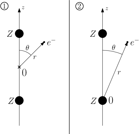
At the same time, for the TC potential the results should be identical within the numerical error bars. We compare two different placements of the c.s. origin: at the center of mass of the nuclei, at the center of one of the nuclei, see Figure 4. The agreement between TC(1) and TC(2) within the anticipated numerical uncertainty serves as a non-trivial self-test of the method, since the basis-set expansion (6) is essentially different for the two cases. In fact, due to the lower symmetry of the second c.s., the uncertainty of the TC(2) values is much larger and completely determines the difference between TC(1) and TC(2). The differences between the TC(1) and MA(1) results are presented in the second-to-last column, they can be interpreted as inaccuracy of the MA. In the last column, the differences between the MA(1) and MA(2) results are given, a kind of ‘‘inherent inconsistency’’ of the MA. As one can see from these data, except for the regions where is anomaly small due to the sign change, it is comparable to . This observation can be used to quantify the inaccuracy of the MA for the contributions, which are not yet available for the TC calculations, e.g., the two-photon-exchange and QED corrections Kotov et al. 2020.
| , fm | ||||||
|---|---|---|---|---|---|---|
| 40 | 646254 | 646254 | 637032 | 598564 | 9222 | 38468 |
| 50 | 614504 | 614504 | 604643 | 568188 | 9861 | 36455 |
| 80 | 550575 | 550575 | 539861 | 506742 | 10714 | 33119 |
| 100 | 521373 | 521373 | 510350 | 478423 | 11023 | 31927 |
| 200 | 433348 | 433347 | 421146 | 392345 | 12202 | 28801 |
| 250 | 405450 | 405450 | 392687 | 365185 | 12763 | 27502 |
| 500 | 319773 | 319769 | 304337 | 283510 | 15436 | 20827 |
| 289068 | 289067 | 272212 | 255389 | 16856 | 16823 | |
| 700 | 279462 | 279464 | 262095 | 246756 | 17367 | 15339 |
| 1000 | 238887 | 238873 | 218905 | 211937 | 19982 | 6968 |
| 212020 | 212003 | 189652 | 190174 | 22368 | 522 |
| , fm | ||||||
|---|---|---|---|---|---|---|
| 40 | 192031 | 192031 | 191860 | 190033 | 171 | 1827 |
| 50 | 190845 | 190845 | 190607 | 188314 | 238 | 2293 |
| 80 | 187217 | 187216 | 186775 | 183199 | 442 | 3576 |
| 100 | 184805 | 184805 | 184228 | 179895 | 577 | 4333 |
| 200 | 173425 | 173425 | 172190 | 165031 | 1235 | 7159 |
| 250 | 168242 | 168242 | 166695 | 158621 | 1547 | 8074 |
| 500 | 146803 | 146802 | 143860 | 133919 | 2943 | 9941 |
| 700 | 133710 | 133710 | 129828 | 120118 | 3882 | 9710 |
| 119414 | 119413 | 114421 | 105971 | 4993 | 8450 | |
| 1000 | 118529 | 118528 | 113464 | 105233 | 5065 | 8231 |
| 89269 | 89276 | 81433 | 79488 | 7836 | 1945 |
IV Discussion and conclusion
In this work, the two-center Dirac equation is solved within the dual-kinetic-balance method Shabaev et al. 2004; Rozenbaum et al. 2014. The energies of the ground and several excited -states in such heavy diatomic systems as Pb82+–Pb82+–e- and Xe54+–Xe54+–e- are plotted as a function of the internuclear distance . The ground-state energies at the ‘‘chemical’’ distances ( a.u.) are presented for one-electron dimers with . Obtained data are compared with the available previous calculations and a good agreement is observed. The comparison of the results for different origin placement of the coordinate system is used as a self-test of the method. The values obtained within the monopole approximation are also presented. It is shown that their dependence on the origin placement can serve to estimate the deviation from the two-center results.
The developed method, in addition to the energies and wave functions of the ground and lowest excited states, provides the quasicomplete finite spectrum. The Green function computed on the basis of this spectrum gives an access, in particular, to evaluation of the Feynman diagrams within the bound-state QED.
Acknowledgements.
Valuable discussions with Ilia Maltsev, Alexey Malyshev, Leonid Skripnikov, and Ilya Tupitsyn are gratefully acknowledged. The work was supported by the Foundation for the Advancement of Theoretical Physics and Mathematics ‘‘BASIS’’, by the Russian Foundation for Basic Research (grant number 19-02-00974), by TU Dresden (DAAD Programm Ostpartnerschaften), and by G-RISC.References
- Gerstein and Zeldovich (1969) S. S. Gerstein and Y. B. Zeldovich, Sov. Phys. JETP 30, 358 (1969).
- Pieper and Greiner (1969) W. Pieper and W. Greiner, Z. Phys. 218, 327 (1969).
- Zeldovich and Popov (1972) Y. B. Zeldovich and V. S. Popov, Sov. Phys. Usp. 14, 673 (1972).
- Rafelski et al. (1978) J. Rafelski, L. P. Fulcher, and A. Klein, Phys. Rep. 38, 227 (1978).
- Greiner et al. (1985) W. Greiner, B. Müller, and J. Rafelski, Quantum Electrodynamics of Strong Fields (Springer-Verlag, Berlin, 1985).
- Maltsev et al. (2019) I. A. Maltsev, V. M. Shabaev, R. V. Popov, Y. S. Kozhedub, G. Plunien, X. Ma, T. Stöhlker, and D. A. Tumakov, Phys. Rev. Lett. 123, 113401 (2019).
- Popov et al. (2020) R. V. Popov, V. M. Shabaev, D. A. Telnov, I. I. Tupitsyn, I. A. Maltsev, Y. S. Kozhedub, A. I. Bondarev, N. V. Kozin, X. Ma, G. Plunien, T. Stöhlker, D. A. Tumakov, and V. A. Zaytsev, Phys. Rev. D 102, 076005 (2020).
- (8) D. N. Voskresensky, arXiv:2102.07182 .
- Verma et al. (2006a) P. Verma, P. Mokler, A. Bräuning-Demian, H. Bräuning, C. Kozhuharov, F. Bosch, D. Liesen, S. Hagmann, T. Stöhlker, Z. Stachura, D. Banas, A. Orsic-Muthig, M. Schöffler, D. Sierpowski, U. Spillmann, S. Tashenov, S. Toleikis, and M. Wahab, Nucl. Instrum. Meth. Phys. Res. B 245, 56 (2006a).
- Verma et al. (2006b) P. Verma, P. Mokler, A. Bräuning-Demian, C. Kozhuharov, H. Bräuning, F. Bosch, D. Liesen, T. Stöhlker, S. Hagmann, S. Chatterjee, A. Gumberidze, R. Reuschl, M. Schöffler, U. Spillmann, A. Orsic Muthig, S. Tachenov, Z. Stachura, and M. Wahab, Radiation Physics and Chemistry 75, 2014 (2006b).
- Hagmann et al. (2011) S. Hagmann, T. Stöhlker, C. Kozhuharov, V. Shabaev, I. Tupitsyn, Y. Kozhedub, H. Rothard, U. Spillmann, R. Reuschl, S. Trotsenko, F. Bosch, D. Liesen, D. Winters, J. Ullrich, R. Dörner, R. Moshammer, P. Hillenbrand, D. Jakubassa‐Amundsen, A. Voitkiv, A. Surzhykov, D. Fischer, E. de Filippo, X. Wang, and B. Wei, AIP Conference Proceedings 1336, 115 (2011).
- Gumberidze et al. (2009) A. Gumberidze, T. Stöhlker, H. Beyer, F. Bosch, A. Bräuning-Demian, S. Hagmann, C. Kozhuharov, T. Kühl, R. Mann, P. Indelicato, W. Quint, R. Schuch, and A. Warczak, Nucl. Instrum. Meth. Phys. Res. B 267, 248 (2009).
- Ter-Akopian et al. (2015) G. M. Ter-Akopian, W. Greiner, I. N. Meshkov, Y. T. Oganessian, J. Reinhardt, and G. V. Trubnikov, International Journal of Modern Physics E 24, 1550016 (2015).
- Ma et al. (2017) X. Ma, W. Wen, S. Zhang, D. Yu, R. Cheng, J. Yang, Z. Huang, H. Wang, X. Zhu, X. Cai, Y. Zhao, L. Mao, J. Yang, X. Zhou, H. Xu, Y. Yuan, J. Xia, H. Zhao, G. Xiao, and W. Zhan, Nucl. Instrum. Meth. Phys. Res. B 408, 169 (2017).
- Soff et al. (1979) G. Soff, W. Greiner, W. Betz, and B. Müller, Phys. Rev. A 20, 169 (1979).
- Becker et al. (1986) U. Becker, N. Grün, W. Scheid, and G. Soff, Phys. Rev. Lett. 56, 2016 (1986).
- Eichler (1990) J. Eichler, Physics Reports 193, 165 (1990).
- Rumrich et al. (1993) K. Rumrich, G. Soff, and W. Greiner, Phys. Rev. A 47, 215 (1993).
- Ionescu and Belkacem (1999) D. C. Ionescu and A. Belkacem, Physica Scripta T80, 128 (1999).
- Tupitsyn et al. (2010) I. I. Tupitsyn, Y. S. Kozhedub, V. M. Shabaev, G. B. Deyneka, S. Hagmann, C. Kozhuharov, G. Plunien, and T. Stöhlker, Phys. Rev. A 82, 042701 (2010).
- Tupitsyn et al. (2012) I. I. Tupitsyn, Y. S. Kozhedub, V. M. Shabaev, A. I. Bondarev, G. B. Deyneka, I. A. Maltsev, S. Hagmann, G. Plunien, and T. Stöhlker, Phys. Rev. A 85, 032712 (2012).
- Müller et al. (1973) B. Müller, J. Rafelski, and W. Greiner, Phys. Lett. B 47, 5 (1973).
- Rafelski and Müller (1976) J. Rafelski and B. Müller, Phys. Lett. B 65, 205 (1976).
- Rafelski and Müller (1976) J. Rafelski and B. Müller, Phys. Rev. Lett. 36, 517 (1976).
- Lisin et al. (1977) V. I. Lisin, M. S. Marinov, and V. S. Popov, Phys. Lett. B 69, 141 (1977).
- Lisin et al. (1980) V. I. Lisin, M. S. Marinov, and V. S. Popov, Phys. Lett. B 91, 20 (1980).
- Yang et al. (1991) L. Yang, D. Heinemann, and D. Kolb, Chem. Phys. Lett. 178, 213 (1991).
- Parpia and Mohanty (1995) F. A. Parpia and A. K. Mohanty, Chem. Phys. Lett. 238, 209 (1995).
- Deineka (1998) G. B. Deineka, Opt. Spectrosc. 84, 159 (1998).
- Matveev et al. (2000) V. I. Matveev, D. U. Matrasulov, and H. Y. Rakhimov, Phys. Atom. Nuclei 63, 318 (2000).
- Kullie and Kolb (2001) O. Kullie and D. Kolb, Eur. Phus. J. D 17, 167 (2001).
- Ishikawa et al. (2008) A. Ishikawa, H. Nakashima, and H. Nakatsuji, J. Chem. Phys. 128, 124103 (2008).
- Artemyev et al. (2010) A. N. Artemyev, A. Surzhykov, P. Indelicato, G. Plunien, and T. Stoehlker, J. Phys. B 43, 235207 (2010).
- Ishikawa et al. (2012) A. Ishikawa, H. Nakashima, and H. Nakatsuji, Chem. Phys. 401, 62 (2012).
- Tupitsyn and Mironova (2014) I. I. Tupitsyn and D. V. Mironova, Opt. Spectrosc. 117, 351 (2014).
- Mironova et al. (2015) D. V. Mironova, I. I. Tupitsyn, V. M. Shabaev, and G. Plunien, Chem. Phys. 449, 10 (2015).
- Artemyev and Surzhykov (2015) A. N. Artemyev and A. Surzhykov, Phys. Rev. Lett. 114, 243004 (2015).
- Shabaev et al. (2004) V. M. Shabaev, I. I. Tupitsyn, V. A. Yerokhin, G. Plunien, and G. Soff, Phys. Rev. Lett. 93, 130405 (2004).
- Rozenbaum et al. (2014) E. B. Rozenbaum, D. A. Glazov, V. M. Shabaev, K. E. Sosnova, and D. A. Telnov, Phys. Rev. A 89, 012514 (2014).
- Kotov et al. (2020) A. A. Kotov, D. A. Glazov, A. V. Malyshev, A. V. Vladimirova, V. M. Shabaev, and G. Plunien, X-Ray Spectrometry 49, 110 (2020).
- Shabaev (1993) V. M. Shabaev, J. Phys. B 26, 1103 (1993).
- Johnson et al. (1988) W. R. Johnson, S. A. Blundell, and J. Sapirstein, Phys. Rev. A 37, 307 (1988).
- Sapirstein and Johnson (1996) J. Sapirstein and W. R. Johnson, J. Phys. B 29, 5213 (1996).
- Varentsova et al. (2017) A. S. Varentsova, V. A. Agababaev, A. M. Volchkova, D. A. Glazov, A. V. Volotka, V. M. Shabaev, and G. Plunien, Nucl. Instrum. Meth. Phys. Res. B 408, 80 (2017).
- Volchkova et al. (2017) A. M. Volchkova, A. S. Varentsova, N. A. Zubova, V. A. Agababaev, D. A. Glazov, A. V. Volotka, V. M. Shabaev, and G. Plunien, Nucl. Instrum. Meth. Phys. Res. B 408, 89 (2017).
- (46) A. M. Volchkova, V. A. Agababaev, D. A. Glazov, A. V. Volotka, S. Fritzsche, V. M. Shabaev, and G. Plunien, arXiv:2009.00109 .