跳到论文正文
W Papers独立论文阅读器 arXiv:2105.05742 论文正文 计算阅读时间 · 0%
引用这篇论文根据当前论文元数据生成,正式投稿前建议核对。


License: arXiv.org perpetual non-exclusive license
arXiv:2105.05742v1 [physics.plasm-ph] 12 May 2021

Zero-dimensional and pseudo-one-dimensional models of atmospheric-pressure plasma jet in binary and ternary mixtures of oxygen and nitrogen with helium background

Youfan He    Patrick Preissing    David Steuer    Maximilian Klich    Volker Schulz-von der Gathen    Marc Böke    Ihor Korolov    Julian Schulze    Vasco Guerra Affiliation:  Instituto de Plasmas e Fusão Nuclear, Instituto Superior Técnico, Universidade de Lisboa, Portugal    Ralf Peter Brinkmann    Efe Kemaneci Email: efekemaneci@gmail.com
Abstract

A zero-dimensional (volume-averaged) and a pseudo-one-dimensional (plug-flow) model are developed to investigate atmospheric-pressure plasma jet devices operated with He, He/O2\mathrm{O_{2}}, He/N2\mathrm{N_{2}} and He/N2\mathrm{N_{2}}/O2\mathrm{O_{2}} mixtures. The models are coupled with the Boltzmann equation under the two-term approximation to self-consistently calculate the electron energy distribution function (EEDF). The simulation results are verified against spatially resolved model calculations and validated against a wide variety of measurement data. The nitric oxide (NO\mathrm{NO}) concentration is thoroughly characterized for a variation of the gas mixture ratio, helium flow rate and absorbed power. The concentration measurements at low power are better captured by the simulation with a larger hypothetical `​```effective"" rate coefficient value for the reactive quenching N2(A3Σ,B3Π)+O(3P)→NO+N(2D)\mathrm{N_{2}(A^{3}\Sigma,B^{3}\Pi)}+\mathrm{O(^{3}P)}\rightarrow\mathrm{NO}+\mathrm{N(^{2}D)}. This suggests that the NO\mathrm{NO} production at low power is also covered by the species N2​(A3​Σ,B3​Π,v>0)\mathrm{N_{2}(A^{3}\Sigma,B^{3}\Pi;}\>v>0) and multiple higher N2\mathrm{N_{2}} electronically excited states instead of only N2​(A3​Σ,B3​Π,v=0)\mathrm{N_{2}(A^{3}\Sigma,B^{3}\Pi;}\>v=0) in this quenching. Furthermore, the O(3P)\mathrm{O(^{3}P)} density measurements under the same operation conditions are also better predicted by the simulations with a consideration of the aforementioned hypothetical rate coefficient value. It is found that the contribution of the vibrationally excited nitrogen molecules N2​(v⩾13)\mathrm{N_{2}}(v\geqslant 13) to the net NO\mathrm{NO} formation rate gains more significance at higher power. The vibrational distribution functions (VDFs) of molecular oxygen O2​(v<41)\mathrm{O_{2}}(v<41) and nitrogen N2​(v<58)\mathrm{N_{2}}(v<58) are investigated regarding their formation mechanisms and their responses to the variation of operation parameters. It is observed that the N2\mathrm{N_{2}} VDF shows a stronger response than the O2\mathrm{O_{2}} VDF. The sensitivity of the zero-dimensional model with respect to a variation of the VDF resolutions, wall reaction probabilities and synthetic air impurity levels is presented. The simulated plasma properties are sensitive to the variation especially for a feeding gas mixture containing nitrogen.

1 Introduction

Atmospheric-pressure plasma jet devices attract growing interest over the last decades owing to their efficiency in converting ordinary gas contents into diverse reactive species for the purposes of biomedical applications [1], catalytic greenhouse gas conversion [2, 3], vacuum-free etching [4] and deposition [5, 6, 7]. The small electrode gap of micro-scaled atmospheric-pressure plasma jet (μ\rm\muAPPJ) ensures the uniformity at low voltage and sustains the characteristics of a glow discharge. The non-equilibrium character permits an efficient electron heating while keeping the neutral species near ambient temperature suitable for the treatment of heat-sensitive materials. An accurate control of the reactive species concentrations is of fundamental importance to achieve an optimized treatment performance.

The atomic structure of the noble gas conduces to ignite and sustain an atmospheric-pressure discharge at a relatively low absorbed power, and helium is being of the preference over argon due to the lower breakdown voltage [8] and higher discharge stability [9]. A wide variety of reactive species are usually generated by an addition of reactive admixtures (e.g., O2, N2 typically in the order of 0-2 %) to the feeding noble gas. A challenge still to be addressed is a full picture of the convoluted plasma chemistry defining the reactive species concentrations. The chemical complexity is attributed to the multitude of interactions between neutral and ion, as well as atomic and molecular species. It is further increased through the introduction of several gases. Therefore, a deep understanding of the rich chemical kinetics is of the essence for a characterization and optimization of the device. In view of this purpose, zero-dimensional modelling approaches [10, 11, 12, 13] are competent to report a detailed chemical description, avoid the resulting drastic computational load and probe the underlying reaction mechanisms efficiently.

Zero-dimensional modelling approaches are implemented either in volume-averaged formalism [10, 11, 13] or in plug-flow formalism [12]. The former gives the volume-averaged plasma properties of the whole chamber, whereas the latter provides those of a small plug-volume by mapping its time-evolution to the spatial-resolution in gas flow direction [14]. The models are used in combination with experiments to investigate the concentrations and chemical kinetics of ozone [12], atomic oxygen and nitric oxide [15], atomic oxygen and hydroxyl radical [16], helium metastable and reactive oxygen species [17], as well as argon metastable, ozone and nitrogen oxide species [18]. However, an effort on the benchmark against a broad range of experimental data (in view of diverse species, operation parameters, measurement techniques) is still missing for an atmospheric-pressure discharge. Such a validation is of crucial significance to further ensure predictive capability of the model calculations.

Nitric oxide (NO) is one of the key species for biomedical applications [19] (e.g., it plays an essential role in wound healing). It has been intensively studied, both experimentally [20, 21, 22, 23, 24, 25] and computationally [13, 12, 18, 26, 27]. The measurements of production rate [20, 21] and absolute density [22] are carried out in a Herriott cell. Spatially resolved densities in the effluent are reported [23, 24]. Similar experiments for a variation of the gas mixture ratio, helium flow rate and absorbed power are recently conducted on the COST Reference Microplasma Jet (COST-Jet) [25]. In this device, the non-reproducibility due to gas contamination and power measurement is minimized by the refinement of the mechanical and electrical design [28]. This is extremely suitable for the benchmark of model calculations. The dominant reaction mechanisms are discussed in simulation studies [13, 18, 26, 27, 15], and the influence of operation parameters on the species concentrations is presented [12]. The NO concentration is characterized by the simulation results and measurement data of a high-pressure discharge [29] and an atmospheric-pressure plasma [15]. Nevertheless, there is still a lack on the validation for a variation of operation parameters.

A detailed resolution of the vibrational distribution function (VDF) has gained much attention in low-pressure plasma [30, 31, 32, 33, 34, 35, 36, 37] (e.g., N2​(v<46)\mathrm{N_{2}}(v<46) [30], O2​(v<42)\mathrm{O_{2}}(v<42) [31, 33]). Its influence on the electron energy distribution function (EEDF) [30, 32, 37, 36, 38] and the plasma properties [31, 33] is presented. An important role of the nitrogen VDF in the production of nitric oxide and nitrogen atom is reported [35, 39], and the VDF is intensively investigated [37]. However, the influence of the detailed VDF on an atmospheric-pressure discharge is not yet fully understood. The vibrationally excited states in the zero-dimensional model are neglected [13, 18, 26] or included with a few vibrational levels [12, 17, 40, 41, 42, 27]. On the other hand, their high excited states are suggested to play a role in the ozone formation [43], and this in turn affects the chemical kinetics of other species. A further study about the detailed VDF and the corresponding vibrational kinetics contributes to a better accuracy of the simulation results.

Wall reactions [11, 13, 17, 40, 41, 16, 44, 45] and gas impurities [11, 13, 12, 17, 40, 41, 16, 26, 27, 15] are usually taken into account in zero-dimensional models due to their underlying effects on the plasma properties. The role of wall reactions is presented such as for a feeding gas mixture of Ar/H2​O\mathrm{H_{2}O} [44] or He/H2​O\mathrm{H_{2}O} [45]. The influence of gas impurities is shown, e.g., on a He [11, 13, 16] or He/O2\mathrm{O_{2}} [17, 40, 41] discharge. In parallel with these studies, the highlight of this work is to make a systematic analysis gradually for several gas mixtures: He, He/O2\mathrm{O_{2}}, He/N2\mathrm{N_{2}} and He/N2\mathrm{N_{2}}/O2\mathrm{O_{2}}.

The main goals of this paper are as follows:

  • •

    For a confirmed prediction capability, the developed zero-dimensional and pseudo-one-dimensional models are well benchmarked against spatially resolved simulation results and numerous measurements data for distinct species densities under different operation conditions from various literature, as shown in section 5.1.

  • •

    The NO concentration in the COST-Jet is intensively characterized by the simulations and experiments for a variation of the gas mixture ratio, helium flow rate and absorbed power (see section 5.2).

  • •

    The role of the detailed resolution of O2​(v<41)\mathrm{O_{2}}(v<41) and N2​(v<58)\mathrm{N_{2}}(v<58) VDFs in an atmospheric-pressure discharge is presented in section 5.4.

The description of the atmospheric-pressure plasma jets simulated in this work is provided in section 2. The developed models are described in section 3 and the considered chemical kinetics are discussed in section 4. The spatial evolution of NO concentration in gas flow direction, and the main gain/loss channels are exhibited in section 5.2. The variation of the VDFs and their spatial evolution to the operation parameters is demonstrated in section 5.3, The sensitivity of the plasma properties to the wall reaction probabilities and the synthetic air (N2\mathrm{N_{2}}:O2\mathrm{O_{2}}=8:2) impurity levels is addressed in section 5.4. The main results are summarized in the conclusion given in section 6.

2 Setup

Atmospheric-pressure plasma jets of planar electrode configuration in five different sizes [46, 47, 48, 49, 50, 51, 52] are simulated for the purpose of benchmark. The specific operation conditions are presented in section 5.1. A plasma jet [48] is investigated as a preliminary test of the model predictive capability to a pulsed-modulated discharge. The old versions of the radio-frequency driven COST-Jet (i.e., a μ\rm\muAPPJ) [47, 49, 50, 52] might be insufficiently sealed. The resulting unknown high impurity levels in the experiments [47] may impact the results and need to be considered in the simulations. Furthermore, a power transfer efficiency around 5 % is usually assumed in the modelling of these old versions for converting the provided generator input power to the absorbed power in the plasma. The irreproducible experimental results of a μ\rm\muAPPJ are mainly ascribed to the gas impurity and the power uncertainty. Hence, they are minimized by the COST-Jet [46, 51] with a large amount of effort [28] (e.g., the sealing improvement and the absorbed power measurements with integrated probes).

The COST-Jet is investigated with a focus in this paper owing to the above-mentioned advantages. In section 5.2, the operation conditions are rightfully addressed based on the measurements of Preissing e​tet a​l.al. [25]. In sections 5.3 and 5.4, the jet is simulated with a typical operation condition provided in [28]: the plasma volume of 1×1×301\times 1\times 30 mm3 sustained by an absorbed power of 0.6 W at a pressure of 101325 Pa and a gas temperature of 345 K, is fed with 1400 sccm He, 1400 sccm He + 0.5% O2\mathrm{O_{2}}, 1400 sccm He + 0.5% N2\mathrm{N_{2}} or 1400 sccm He + 0.5% N2\mathrm{N_{2}} + 0.5% O2\mathrm{O_{2}}, unless stated otherwise. The computational method for a prediction of the plasma properties in the aforementioned setups is explained by the physical and chemical model in section 3 and 4, respectively.

3 Model

The species particle balance equations and an electron energy balance equation are incorporated in the model to calculate the plasma properties: the species concentrations and an effective electron temperature Te{\rm T}_{\rm e} (eV). The electron density is calculated by imposing a constraint on its wall flux based on the quasi-neutrality implementation [53], and the gas temperature value Tg{\rm T}_{\rm g} (K) is fixed by the measurements. Both the zero-dimensional volume-averaged formalism [10, 11] and the pseudo-one-dimensional plug-flow formalism [14, 12, 16] are implemented. The balance equations are averaged over the whole plasma domain in the zero-dimensional formalism, and steady or transient volume-averaged plasma quantities are calculated [54, 55]. In the pseudo-one-dimensional formalism, the equations are averaged over a much smaller plug-volume, that is infinitesimally small along the unidirectional laminar net mass flow field. The time-evolution in this volume is mapped to the spatial position in the discharge channel since the plug co-moves with the net mass flow.

The EEDF is calculated based on the steady-state solution of the Boltzmann equation under the two-term approximation. The open-source simulation tool LisbOn KInetics Boltzmann (LoKI-B) published by Tejero-del-Caz e​tet a​l.al. [56] is adapted for a self-consistent calculation. Super-elastic collisions are incorporated in the calculation for a better resolution of the electron kinetics [57, 58, 59]. The time-variation of the plasma composition in the transient simulations (e.g., pulse-modulated zero-dimensional and pseudo-one-dimensional models) necessitates multiple subsequent LoKI-B calculations to involve the corresponding evolution of the electron kinetics. However, the electron kinetics is mainly controlled by the virtually invariant dominant background helium gas density. This is furthermore confirmed by the insensitivity of the simulation results to the number of calling LoKI-B (multiple during the pulse/plug-flow or single in-advance). In order to reduce the computationally-demanding transient simulation duration, LoKI-B is deployed in advance by a single call to calculate the EEDF for a corresponding steady-state plasma composition.

A time-dependent solution of the Boltzmann equation would better represent the transient phenomena [37]. However, at atmospheric pressure, the time necessary to establish a steady-state EEDF is in the order of nanoseconds, approximated by the reduced momentum-transfer collision frequency. The range of the value is also numerically verified (e.g., a few nanoseconds in the kinetic models [57]). Therefore, the stationary solution of the Boltzmann equation is considered in the transient simulations (microsecond-pulsed modulation) of this work, in parallel with the available implementations of time-dependent (nanosecond range) models [60, 61, 62].

The generic form of the volume-averaged particle balance equation is

d​nid​t=∑j𝒲i​j​Rij|V+∑j𝒲i​j​Rij|W,\frac{dn_{i}}{dt}=\left.\sum_{j}{\cal W}_{ij}R^{j}_{i}\right|_{V}+\left.\sum_{j}{\cal W}_{ij}R^{j}_{i}\right|_{W}, (1)

where nin_{i} is the volume-averaged density of the species denoted by ii, 𝒲i​j{\cal W}_{ij} is the net stoichiometric coefficient for a gain/loss mechanism denoted by jj, and RijR^{j}_{i} is the reaction rate. The subscript “V” denotes the chemical reactions inside the plasma volume and “W” the flux (e.g., convective and diffusive) source term including the heterogeneous reactions on the solid walls.

The rate of a plasma volume chemical reaction jj is

Rij|V=kj​∏lnlνl​j,\left.R^{j}_{i}\right|_{V}=k^{j}\prod_{l}n_{l}^{\nu_{lj}}, (2)

where kjk^{j} is the rate coefficient, ll the reactant and νl​j\nu_{lj} is the forward stoichiometric coefficient. The rate coefficients are tabulated in A. The electronic rate coefficients are mostly computed from the enlisted set of cross-sections available in the literature together with the self-consistently calculated EEDF.

The flow-in and flow-out rates are excluded in the pseudo-one-dimensional formalism due to the motion of the plug with the net mass flow [14]. The flow-in rate in the zero-dimensional formalism is given by the relation [63]

RHe,O2,N2F−in|W=c​QHe,O2,N2​PatmV​kB​Tin,\left.R_{{\rm He,O}_{2}{\rm,N}_{2}}^{{\rm F-in}}\right|_{W}=c\frac{Q_{{\rm He,O}_{2}{\rm,N}_{2}}P_{{\rm atm}}}{V{\rm k}_{B}T_{{\rm in}}}, (3)

where QHe,O2,N2Q_{{\rm He,O}_{2}{\rm,N}_{2}} (sccm) is the partial mass flow rate of each species fed into the plasma domain, PatmP_{{\rm atm}} the atmospheric pressure, VV the plasma volume, TinT_{{\rm in}} the feeding gas temperature and cc is the unit conversion factor. The flow-out rate of a species ii is [63]

RiF−out|W=c​Q​Patm​TgV​P​Tin​ni,\left.R_{i}^{{\rm F-out}}\right|_{W}=cQ\frac{P_{{\rm atm}}{\rm T}_{\rm g}}{VPT_{{\rm in}}}n_{i}, (4)

where QQ denotes the total mass flow rate and PP the plasma pressure.

The ion and neutral wall flux at the surfaces perpendicular to the mass flow field is ignored in the zero-dimensional formalism due to the negligibly small area (mostly forming below 2 % of the total plasma surface area). This term is also neglected in the pseudo-one-dimensional formalism since the convective mass flow mechanism prevails the flux vector [14]. The wall loss of an ion ii at the surfaces parallel to the mass flow field is defined as [55, 64, 65]

Ri+|W=(ui​B​hi​X+​2​AXfVf+ui​B​hi​Y+​2​AYfVf)​ni,R^{+}_{i}\left.\right|_{W}=\left(u_{iB}\frac{h^{+}_{iX}2A^{f}_{X}}{V^{f}}+u_{iB}\frac{h^{+}_{iY}2A^{f}_{Y}}{V^{f}}\right)n_{i}, (5)

where ui​Bu_{iB} denotes the Bohm velocity, hi​X+h^{+}_{iX} and hi​Y+h^{+}_{iY} are the ion edge-to-center ratios, the superscript f specifies either the zero-dimensional or the pseudo-one-dimensional implementation, VfV^{f} is the corresponding volume, AXfA^{f}_{X} and AYfA^{f}_{Y} are their surface areas. Namely, the values of VfV^{f},AXfA^{f}_{X} and AYfA^{f}_{Y} are either the plasma volume and surface in the zero-dimensional formalism, or the plug volume and surface in the pseudo-one-dimensional formalism.

The edge-to-center ratio definition is adapted in the ion wall flux, following conventional global model studies [66, 67]. It should be noted that the edge-to-volume-averaged ratio [68] physically represents a more realistic description at intermediate- or atmospheric-pressure (so-called collisional regime [64]), however the resulting variations in the calculations are numerically negligible [55]. The ion velocity at the plasma-sheath edge is expected to deviate from the Bohm velocity at high pressure values due to the larger collisionality of the sheath region compared to the low-pressure plasma [69]. Nevertheless, the deviation is negligible at atmospheric-pressure since the ratio of the ion-neutral collision to the direct ionization frequencies of the helium atomic ion is less than the critical value of 1010 (larger values represent the transition into the collisional sheath regime) based on the analyses by Franklin [69] and Valentini e​tet a​l.al. [70, 71]. Additionally, assuming an effective ionization frequency to include the space-charge dominating excimer ions as well as the prevailing mechanisms of Penning and stepwise ionization schemes lead to a much smaller ratio compared to the critical value. In other words, the validity range of the Bohm criterion is not breached at atmospheric-pressure. Furthermore, our model calculations are not sensitive to the ion wall loss, hence any deviation from the Bohm velocity is not influential on the simulation results.

The ion edge-to-center ratios in the collisional regime are defined as [64, 55]

hi​X+=11+α(ui​B​E/ui​B)(1+(X​ui​B​Eπ​Di+)2)−1/2,hi​Y+=11+α(ui​B​E/ui​B)(1+(Y​ui​B​Eπ​Di+)2)−1/2,\begin{array}[]{l l}h^{+}_{iX}&=\frac{1}{1+\alpha}(u_{iBE}/u_{iB})\left(1+\left(\frac{Xu_{iBE}}{\pi D_{i+}}\right)^{2}\right)^{-1/2},\\ \\[-4.0pt] h^{+}_{iY}&=\frac{1}{1+\alpha}(u_{iBE}/u_{iB})\left(1+\left(\frac{Yu_{iBE}}{\pi D_{i+}}\right)^{2}\right)^{-1/2},\end{array} (6)

where α\alpha represents the degree of electronegativity, ui​B​Eu_{iBE} the electronegative Bohm velocity [72, 73], ui​Bu_{iB} the electropositive Bohm velocity, XX and YY the plasma dimensions, and Di+D_{i+} denotes the multiple-ion ambipolar diffusion coefficient [54].

The reaction rate due to diffusion of a reactive neutral ii to the wall and its subsequent heterogeneous reaction in the zero-dimensional and pseudo-one-dimensional formalisms is given as [74, 75]

RiN|W=ni​(Λ02Di+2​Vf​(2−γi)2​(AXf+AYf)​vi​γi)−1,\left.R^{N}_{i}\right|_{W}=n_{i}\left(\frac{\Lambda_{0}^{2}}{D_{i}}+\frac{2V^{f}(2-\gamma_{i})}{2(A^{f}_{X}+A^{f}_{Y})v_{i}\gamma_{i}}\right)^{-1}, (7)

where Λ0\Lambda_{0} is the effective diffusion length, DiD_{i} the diffusion coefficient, VfV^{f} the volume, 2​(AXf+AYf)2(A^{f}_{X}+A^{f}_{Y}) the net surface area, viv_{i} the mean neutral velocity and γi\gamma_{i} is the wall reaction probability. The superscript f denotes the corresponding parameters in the considered formalism: either those of the plasma in the zero-dimensional or those of the plug in the pseudo-one-dimensional formalism.

The volume-averaged electron energy balance equation is given in the form

dd​t​(32​ne​Te)=Qabs−(QChe+QEla+QW),\frac{d}{dt}\left(\frac{3}{2}n_{e}\mathrm{T_{e}}\right)=Q_{{\rm abs}}-(Q_{{\rm Che}}+Q_{{\rm Ela}}+Q_{\rm W}), (8)

where nen_{e} represents the electron density, Te\mathrm{T_{e}} the effective electron temperature, QabsQ_{{\rm abs}} the electrical power absorbed by the plasma as well as the energy loss due to chemical reactions QCheQ_{{\rm Che}}, elastic collisions QElaQ_{{\rm Ela}} and wall flux QWQ_{\rm W}.

The power absorbed by the plasma, assuming a homogeneous distribution, is defined by the relation

Qabs=β​𝒫/V,Q_{{\rm abs}}=\beta{\mathcal{P}}/V, (9)

where 𝒫{\mathcal{P}} is the input power, VV the plasma volume and β\beta is the power transfer efficiency. The electron energy loss in the chemical reactions is given in the following form

QChe=∑jℰj​Rej|V,Q_{{\rm Che}}=\left.\sum_{j}{\cal E}_{j}R^{j}_{e}\right|_{V}, (10)

where RejR^{j}_{e} denotes the rate of an electronic reaction jj and ℰj{\cal E}_{j} the net energy. The principle of detailed balancing is used in calculating the backward rate coefficients of the electron-impact excitation reactions [64]. The energy loss due to elastic collisions QElaQ_{{\rm Ela}} is calculated by the individual elastic rate coefficients [54, 53]. The considered elastic collisions are tabulated in 14 with a reference to the considered cross-section. The energy loss due to the wall flux is given in the form [55, 64]

QW=∑i∈I​o​n​s(ℰP+ℰe+ℰs)​Ri+|W,Q_{W}=\left.\sum_{i\in Ions}\left({\cal E}_{P}+{\cal E}_{e}+{\cal E}_{s}\right)R^{+}_{i}\right|_{W}, (11)

where ℰP{\cal E}_{P} is the plasma potential, ℰe{\cal E}_{e} is the mean energy loss per electron lost and ℰs{\cal E}_{s} represents the sheath potential. The electron energy balance equation is identically implemented in the zero-dimensional and the pseudo-one-dimensional formalism. The only distinction is the aforementioned calculation of the ion wall loss rate due to the differing volume and surface area.

4 Chemical kinetics

The gas mixtures He, He/O2, He/N2 and He/N2/O2 are considered in this study. The species, reactions and elastic collision sets are enlisted in A: tables 2,3,4,5,6,7,8,9,10,11,12,13 and 14. The reactions are separated into several tables for the sake of clarity and tabulated according to the mixture composition and reaction type. The bulk of the He and He/O2 chemical sets is adopted from a study of Waskoenig e​tet a​l.al. [49], except the vibrational kinetics. This maximizes the consistency in model-to-model benchmark of our zero-dimensional simulation results to that of the one-dimensional model provided by Waskoenig e​tet a​l.al. (see section 5.1). Comparatively, the chemical sets here are supplemented with the reaction mechanisms of O4+\mathrm{O_{4}^{+}} and O4−\mathrm{O_{4}^{-}} for a better agreement of the calculated O(3P)\mathrm{O(^{3}P)} density with the measurement (especially, due to reactions 49, 73 and 74 in table 4). Additionally, more detailed helium excimer reaction mechanisms are included in this work. The chemical sets of He/N2 and He/N2/O2 are established based on a wide variety of studies available in literature (explicitly given in A). Both available databases [76, 77] and individual studies (e.g., [78, 79, 80, 81, 82, 83]) are referred in the data collection. A recent set of electron-impact cross-sections are adopted for N2O and NO2 [84].

The vibrationally excited molecules O2​(v<41)\mathrm{O_{2}}(v<41) and N2​(v<58)\mathrm{N_{2}}(v<58) are incorporated in the species set. The detailed vibrational kinetics in tables 7,8,9,10 and 11 are divided into electron-Vibrational (e-V), Vibrational-Translational (V-T) and Vibrational-Vibrational (V-V) energy transfer mechanisms, mainly based on databases [85, 86] and studies [87, 88, 35, 82, 33, 30]. Moreover, the Penning ionization and charge exchange reactions between helium and vibrationally excited molecules are integrated into the kinetics. The resonant vibrational excitation cross-sections [87, 88] are favoured in the e-V transfer due to their efficiency. Only the cross-sections of the first six vibrational levels are used in the solution to the Boltzmann equation, while those of the higher levels are directly evaluated to the corresponding rate coefficients according to the established EEDF. The reverse rate coefficients of all the e-V excitation are calculated via the principle of detailed balancing [64]. The V-T transitions are substantially dominated by the strong He background gas, however the transitions due to O(3P)\mathrm{O(^{3}P)}, N(4S)\mathrm{N(^{4}S)}, O2 and N2 are considered as well. The rate coefficients of N(v>0)2{}_{2}(v>0)-O2 and O(v>0)2{}_{2}(v>0)-N2 V-T reactions are estimated by those of N(v>0)2{}_{2}(v>0)-N2 and O(v>0)2{}_{2}(v>0)-O2, respectively due to lack of data [35, 30]. Only the N(v>0)2{}_{2}(v>0)-N channel is taken into account among the nitrogen atom induced V-T mechanisms, whereas the inefficient O(v>0)2{}_{2}(v>0)-N channel is neglected [30]. Furthermore, the dissociation mechanism of O(3P)\mathrm{O(^{3}P)} + O(v>0)2{}_{2}(v>0) [89] and the NO formation reaction of O(3P)\mathrm{O(^{3}P)} + N(v⩾13)2{}_{2}(v\geqslant 13) [30] are involved in the calculations. The ozone production channel of O2 + O(v>0)2{}_{2}(v>0) [43] is ignored due to the insensitivity of the simulation results to its presence. The V-V mechanisms are thoroughly considered, however N2​(v⩾0)+O2​(w>1)→N2​(v+1)+O2​(w−1){\rm N}_{2}(v\geqslant 0)+{\rm O}_{2}(w>1)\rightarrow{\rm N}_{2}(v+1)+{\rm O}_{2}(w-1) is excluded on account of its inefficient contribution to the quenching of O(w>0)2{}_{2}(w>0) [90]. Both O2​(v′=41){\rm O}_{2}(v^{\prime}=41) and N2​(v′=58){\rm N}_{2}(v^{\prime}=58), referred as pseudo levels, are assumed to instantaneously dissociate due to the proximity of the vibrational energy to the dissociation energy [91]. In total, the He/N2\mathrm{N_{2}} set includes 7272 distinct species and 58315831 reactions, the He/O2\mathrm{O_{2}} set 5858 species and 32163216 reactions and the He/N2\mathrm{N_{2}}/O2\mathrm{O_{2}} set 138 species and 1179911799 reactions.

The considered neutral and ion reactions at the wall are tabulated in 12 and 13, respectively. The quenching of the excited states and the recombination of nitrogen atom on the chamber surface are taken into account. The oxygen atom wall recombination is ignored since volume processes are expected to dominate over surface reactions under the considered operation conditions [49]. Nevertheless, the influence of the recombination probability value on the simulation results is discussed in section 5.1. An ion impinging on the surface is assumed to capture an electron via the Auger effect or resonant electron transfer and then returns back to the plasma region.

By modifications of the underlying production channels based on the above-mentioned reference chemical kinetics, four sets of additional analyses are conducted on the NO density in He/N2/O2 mixtures (see section 5.2):

  1. (1)

    A rate coefficient value of 1×10−191\times 10^{-19} m3/s\mathrm{m^{3}/s} is used for the reaction O(3P)+N2(v⩾13)→NO+N(4S)\mathrm{O(^{3}P)}+\mathrm{N_{2}}(v\geqslant 13)\rightarrow\mathrm{NO}+\mathrm{N(^{4}S)} in this study, suggested by Guerra e​tet a​l.al. [35, 34, 30] and Pintassilgo e​tet a​l.al. [92]. A distinct value of 1×10−171\times 10^{-17} m3/s\mathrm{m^{3}/s} is used by Gordiets e​tet a​l.al. [93] and the influence of this value on the NO density is quantified.

  2. (2)

    A NO wall formation by the adsorbed O(3P)\rm O(^{3}P) and N(4S)\rm N(^{4}S) on the surface is ignored due to negligible probability measured at a lower pressure regime [94]. However, the probability is not confirmed for atmospheric-pressure plasma jets. The presence of a NO wall formation N(4S)+wall→NO\rm N(^{4}S)+wall\rightarrow NO (i.e., an effective form of the surface reactions given by a set of adsorbed layer reaction mechanisms [95]) is further considered with a maximum probability of 1 based on set (1), and its role in the NO density is shown. This wall reaction is constructed under the presumption that O(3P)\rm O(^{3}P) is sufficiently adsorbed on the surface due to its much larger concentration compared to that of N(4S)\rm N(^{4}S) under the considered operation conditions.

  3. (3)

    A well accepted value of 7×10−187\times 10^{-18} m3/s\mathrm{m^{3}/s} [82, 30, 81] is used for the reactive quenching N2(A3Σ)+O(3P)→NO+N(2D)\rm N_{2}(A^{3}\Sigma)+O(^{3}P)\rightarrow NO+N(^{2}D) in this work. The value is confirmed for the vibrational ground state N2​(A3​Σ,v=0)\mathrm{N_{2}(A^{3}\Sigma},v=0). Note that a much larger value is observed for the higher vibrational quantum numbers N2​(A3​Σ,v>0)\mathrm{N_{2}(A^{3}\Sigma},v>0) [96, 97, 98, 99, 100, 101]. Furthermore, the virtually identical NO density is obtained between the measurements and the simulations considering the reactive quenching of multiple N2\mathrm{N_{2}} electronically excited states by O(3P)\mathrm{O(^{3}P)} [29]. In order to estimate the role of the vibrationally excited molecules N2​(A3​Σ,v>0)\mathrm{N_{2}(A^{3}\Sigma},v>0) and of multiple higher N2\mathrm{N_{2}} electronically excited states, a larger hypothetical rate coefficient value of 7×10−157\times 10^{-15} m3/s\mathrm{m^{3}/s} is considered for the aforementioned quenching reaction and the resulting NO density is revealed.

  4. (4)

    A reactive quenching of N2​(B3​Π)\mathrm{N_{2}(B^{3}\Pi)} by O(3P)\mathrm{O(^{3}P)} is neglected in many chemical kinetics studies [83, 82, 30, 81, 13] except a handful of publications [102, 103, 29] assigning a rate coefficient value of 3×10−163\times 10^{-16} m3/s\mathrm{m^{3}/s}. On the other hand, larger quenching rates of N2​(B3​Π,v>0)\mathrm{N_{2}(B^{3}\Pi},v>0) are observed at its higher vibrational levels [104]. Thus, the same hypothetical rate coefficient value of 7×10−157\times 10^{-15} m3/s\mathrm{m^{3}/s} for the reactive quenching N2(B3Π)+O(3P)→NO+N(2D)\rm N_{2}(B^{3}\Pi)+O(^{3}P)\rightarrow NO+N(^{2}D) is additionally included to estimate the role of N2​(B3​Π,v⩾0)\mathrm{N_{2}(B^{3}\Pi},v\geqslant 0) and of multiple higher N2\mathrm{N_{2}} electronically excited states based on set (3). Their influence on the NO concentration is presented.

It should be noted that the state-by-state resolution of the vibrational distribution function N2​(A3​Σ,B3​Π,v>0)\mathrm{N_{2}(A^{3}\Sigma,B^{3}\Pi;}\>v>0) is not preferred in the current study due to lack of the necessary data and the excessive computational load. Moreover, the kinetics of the above-mentioned multiple N2\mathrm{N_{2}} electronically excited states are intensively discussed in a nanosecond-pulsed air discharge at a pressure of 13332 Pa [29]. Compared to the measured peak NO\mathrm{NO} density, a factor of ∼\sim5 is under-estimated by the simulations considering the reactive quenching of N2​(A3​Σ,B3​Π,C3​Π)\mathrm{N_{2}(A^{3}\Sigma,B^{3}\Pi,C^{3}\Pi)} by O(3P)\mathrm{O(^{3}P)}. The under-estimation is minimized by an introduction of the triplet states N2​(W3​Δu,B′​Σu−3,E3​Σg+)\mathrm{N_{2}(W^{3}\Delta_{u},B^{\prime}{}^{3}\Sigma^{-}_{u},E^{3}\Sigma^{+}_{g})} and the singlet states N2​(a′​Σu−1,a1​Πg,w1​Δu,a′′​Σg+1)\mathrm{N_{2}(a^{\prime}{}^{1}\Sigma^{-}_{u},a^{1}\Pi_{g},w^{1}\Delta_{u},a^{\prime\prime}{}^{1}\Sigma^{+}_{g})} in this quenching with a gas kinetic rate coefficient value of 3×10−163\times 10^{-16} m3/s\mathrm{m^{3}/s} (except that of N2​(A3​Σ)\mathrm{N_{2}(A^{3}\Sigma)} with ∼\sim10-18 m3/s\mathrm{m^{3}/s}). The role of these multiple higher electronically excited states is partially estimated in our study by the hypothetically large rate coefficient value of 7×10−157\times 10^{-15} m3/s\mathrm{m^{3}/s} in sets (3) and (4). An `​```effective"" value of 1.5×10−151.5\times 10^{-15} m3/s\mathrm{m^{3}/s} for set (4) can be suggested by the aforementioned factor of ∼\sim5 (observed in [29]). However, the NO density is still under-estimated by our simulations using this value relative to the measurements at low power (e.g., by a factor of around 2 at 0.6 W). Although 7×10−157\times 10^{-15} m3/s\mathrm{m^{3}/s} is evidently not regarded as a realistic rate coefficient value for the reactive quenching channels of N2​(A3​Σ,B3​Π)\mathrm{N_{2}(A^{3}\Sigma,B^{3}\Pi)} in set (4), a strong signal is imposed that their vibrationally excited levels and the multiple higher N2\mathrm{N_{2}} electronically excited states play an underlying role in the NO formation at low power. A development of the chemical kinetics involving these levels and states is desirable in the future.

The sensitivity of the simulation results with respect to the considered wall reaction mechanisms is investigated. A small oxygen atom wall recombination probability value is observed by Booth e​tet a​l.al. [105] at relatively low pressure values; however, the measurements in the considered pressure regime are still absent. Furthermore, a much larger value is assigned by a study of an atmospheric-pressure plasma jet by Schröter e​tet a​l.al. [16], in contradiction with the negligible value suggested by Waskoenig e​tet a​l.al. [49]. Likewise, based on the estimated values at low-pressure plasma sources [106, 107, 108], it is assumed that the ozone wall formation is negligible under the considered operation conditions. The influence of the oxygen and nitrogen atom wall recombination as well as the first-order ozone wall formation probabilities are analysed in section 5.4.

5 Results

The developed models in section 3 and 4 are firstly benchmarked against the spatially resolved simulation results and a wide variety of measurements available from literature [46, 47, 48, 49, 50, 51, 52]. The NO concentration is then characterized with a focus on the comparison between the model calculations and the recently published measurements [25]. Lastly, the VDFs, the wall reaction probabilities and the synthetic air impurity levels are computationally investigated based on the validity of the models. In this section, a pressure of 101325 Pa and a gas temperature of 345 K is used in the simulations, unless stated otherwise.

5.1 Benchmark against measurements and simulation results

Refer to caption
Refer to caption
Figure 1: (a)(a) The volume-averaged electron density (▲\blacktriangle) in a He COST-Jet reported by Golda e​tet a​l.al. [46] and the zero-dimensional simulation results (). (b)(b) The measurements of helium metastable density close to the powered electrode (■\blacksquare) in a He μ\rm\muAPPJ by Niermann e​tet a​l.al. [47] as well as the zero-dimensional simulation results for pure helium () and helium diluted by a linearly decreasing synthetic air (N2:O2=8:2) impurity between 100−10100-10 ppm with respect to the increasing helium flow rate from 500 sccm to 4500 sccm (). We refer to the text for the operation conditions.

The volume-averaged electron density in a He COST-Jet is reported by Golda e​tet a​l.al. [46]. The plasma is operated at a net mass flow rate of 10001000 sccm and a pressure of 99000 Pa. The gas temperature is fixed at about 345345 K [28]. Similar density values and trend are observed between the reported electron density and the zero-dimensional simulation results shown in figure 1(a)(a). Compared with the simulations for an assumption of a Maxwellian EEDF (not shown here), the self-consistent EEDF calculation reduces the electron density (around 28 %) and increases the electron temperature (about from 2.02.0 eV to 2.52.5 eV) due to the depletion in the EEDF tail. It should be emphasized that the electron density is associated with much less susceptibility to the impurities relative to the other species (e.g., helium metastable). Furthermore, the plasma source under investigation is tightly controlled during the measurements to achieve a maximum purity.

The helium metastable density measurements taken close to the powered electrode (i.e., highest density value) in a He μ\rm\muAPPJ with dimensions 1×1.8×401\times 1.8\times 40 mm3 are provided by Niermann e​tet a​l.al. [47]. The fed helium gas flow rate value ranges from 500500 sccm to 45004500 sccm at a pressure of 1×1051\times 10^{5} Pa. The gas temperature is estimated as 333333 K. An input power of 2323 W is fed into the discharge and a power transfer efficiency of 5%5\>\% is assumed in the simulations. Both pure helium and helium with a linearly decreasing synthetic air impurity between 100−10100-10 ppm with respect to the increasing helium flow rate are simulated due to either the back diffusion from the effluent [109] or the air leakage into the feeding gas. The metastable density measurement data and the zero-dimensional simulation results are shown in figure 1(b)(b). The Penning ionization is a significant loss mechanism, and an almost two orders of magnitude smaller metastable density is predicted by the simulations in the presence of the impurity compared with that of pure helium. Note that the inverse-exponentially increasing trend of the measured metastable density can be better explained by the simulation results considering an exponentially decreasing impurity (due to the unknown exponential factor, the results are not shown here). This suggests that the impurity levels are strongly correlated with the feeding gas flow rate.

Refer to caption
Refer to caption
Figure 2: The measurements of He⁡(23​S)\mathrm{He(2^{3}S)} and He2∗\mathrm{He_{2}^{*}} densities (symbols) in a He atmospheric-pressure plasma jet by Nayak e​tet a​l.al. [48] together with the zero-dimensional simulation results. (a)(a) The peak He⁡(23​S)\mathrm{He(2^{3}S)} density between the electrodes (□\square) and its spatially-averaged value (■\blacksquare) in a continuous power input as well as the volume-averaged simulation results (). (b)(b) The time-resolved peak He⁡(23​S)\mathrm{He(2^{3}S)} (□\square) and He2∗\mathrm{He_{2}^{*}} (∘\circ) density measurements in a pulse-modulated power input () as well as the zero-dimensional simulation results for He⁡(23​S)\mathrm{He(2^{3}S)} () and He2∗\mathrm{He_{2}^{*}} (). We refer to the text for the operation conditions.

The helium metastable density in a He atmospheric-pressure plasma jet for both continuous and pulse-modulated power input is measured by Nayak e​tet a​l.al. [48]. The plasma is confined in a volume of 2×9.5×19.12\times 9.5\times 19.1 mm3 with a mass flow rate of 50005000 sccm He at a gas temperature of around 335335 K. An absorbed power of 1515 W is measured in the continuous discharge. The pulse-modulation is applied in a period of 100​μ100\>\mus at a power-on duration of 20​μ20\>\mus and a peak power of around 1515 W. The peak (inter-electrode) and the spatially-averaged He⁡(23​S)\mathrm{He(2^{3}S)} density measurements for the continuous power input as well as the corresponding zero-dimensional simulation results for a variation of the absorbed power are shown in figure 2(a)(a). A linearly increasing He⁡(23​S)\mathrm{He(2^{3}S)} density profile is observed in the simulations with respect to the power. The simulation results represent the volume-averaged density and show a better proximity to the spatially-averaged measurement value than that of the peak. The time-resolved peak He⁡(23​S)\mathrm{He(2^{3}S)} and He2∗\mathrm{He_{2}^{*}} density measurements as well as the simulation results during a modulation cycle in the pulsed operation are shown in figure 2(b)(b). Relative to the measurements, the simulations suggest a slightly smaller He(232^{3}S) density. Note that only the peak density measurements between the electrodes are provided by Nayak e​tet a​l.al.. The spatially-averaged measurements would show a better agreement with the simulations. The over-estimated He2∗\mathrm{He_{2}^{*}} density in the calculations relative to the peak measurements can be partially attributed to the role of the humid air impurities reported by Nayak e​tet a​l.al.. An inclusion of 1010 ppm synthetic air impurity in this work reduces the simulated He2∗\mathrm{He_{2}^{*}} density by a factor of about 0.150.15 (He⁡(23​S)\mathrm{He(2^{3}S)} density about 0.25). Hence, this inclusion improves the agreement between the simulations and the spatially-averaged measurements.

Refer to caption
Refer to caption
Figure 3: The one-dimensional (1-D) spatially resolved simulation results (the time- and space-averaged electron density (▲\blacktriangle) and temperature () as well as the oxygen atom density (■\blacksquare) in the discharge center) and the corresponding oxygen atom density measurements (□\square) in a He/O2\mathrm{O_{2}} μ\rm\muAPPJ by Waskoenig e​tet a​l.al. [49] together with the calculations (lines) by the zero-dimensional (0-D) model for a variation of the absorbed power. (a)(a) electron density and temperature, (b)(b) oxygen atom density. We refer to the text for the operation conditions.

A spatially resolved one-dimensional (1-D) model is developed and its simulation results together with a set of oxygen atom density measurements in a He/O2\mathrm{O_{2}} μ\rm\muAPPJ are reported by Waskoenig e​tet a​l.al. [49]. The plasma dimensions are given as 1×1×401\times 1\times 40 mm3 at a fixed gas temperature value of 345345 K and a pressure of 1×1051\times 10^{5} Pa. A total mass flow rate of 10001000 sccm helium and oxygen is fed into the plasma domain with the ratio 1000:5. A power transfer efficiency of 5%5\>\% is calculated. The simulation results and the measurements are shown in figure 3(a)(a): the time- and space-averaged electron density and temperature calculated by Waskoenig’s one-dimensional simulation as well as our zero-dimensional model, 3(b)(b): the oxygen atom density measurements in the discharge center as well as the one- and zero-dimensional model calculations. The zero-dimensional simulation results for an assumed and maximum oxygen atom wall recombination probability (see reaction 9 in table 12) are also provided in figure 3(b)(b). It should be emphasized that the deviations between the simulation results of both models are ascribed to the supplement of O4+\mathrm{O_{4}^{+}} and O4−\mathrm{O_{4}^{-}} into the zero-dimensional calculations for an improved chemical description. A much better agreement of electron temperature and oxygen atom density is achieved without this supplement. Furthermore, the oxygen atom concentration is over-estimated by both modeling approaches relative to the measurements. This over-estimation is minimized with the assumed wall recombination probability of 0.003. The electron density and temperature calculations are negligibly altered for a variation of the wall recombination probability between a maximum and a vanishing value, below 2 %. Furthermore, the simulation results are not highly sensitive to the exclusion of the vibrationally excited levels. The absence of these levels (not shown here) raises the oxygen atom density by 5.74 %, the electron density by 5.23 %, whereas it reduces the electron temperature by 0.39 %.

Refer to caption
Refer to caption
Refer to caption
Figure 4: The spatially resolved measurements in gas flow direction of a He/O2\mathrm{O_{2}} μ\rm\muAPPJ by Bibinov e​tet a​l.al. [50] as well as both the zero-dimensional (0-D) and pseudo-one-dimensional (pseudo 1-D) simulation results. (a)(a) oxygen atom, (b)(b) ozone and (c)(c) electron densities. We refer to the text for the operation conditions.

The spatial variation of the oxygen atom, ozone and electron densities in gas flow direction is measured inside the chamber of a He/O2\mathrm{O_{2}} μ\rm\muAPPJ by Bibinov e​tet a​l.al. [50]. The plasma is formed within a volume of 1×1.3×401\times 1.3\times 40 mm3 at a gas temperature of 370370 K. The helium and oxygen mass flow rates are fixed at 15001500 sccm and 22.522.5 sccm, respectively. An input power of 3030 W is fed into the plasma and a power transfer efficiency of 55 % is assumed. The measurements together with the simulation results for both the pseudo-one-dimensional plug-flow and the zero-dimensional modelling formalisms are displayed in figure 4. The calculated pseudo-one-dimensional densities are in agreement with the measurements. A close proximity is obtained between the simulation results of both models, e.g., the spatial averages of the pseudo-one-dimensional results are virtually identical with the zero-dimensional results.

Refer to caption
Refer to caption
Figure 5: The measurements (symbols) and the zero-dimensional simulation results (lines) in He/N2\mathrm{N_{2}} μ\rm\muAPPJs. (a)(a) The space- and time-averaged helium metastable density measurements (□\square,■\blacksquare) by Korolov e​tet a​l.al. [51, 110]. (b)(b) The nitrogen atom density measurements () in the effluent (at 4 mm away from the jet nozzle) by Schneider e​tet a​l.al. [52]. We refer to the text for the operation conditions.

The space- and time-averaged helium metastable density measurements in a He/N2\mathrm{N_{2}} COST-Jet are reported by Korolov e​tet a​l.al. [51, 110]. The plasma jet is operated at a pressure of about 1×1051\times 10^{5} Pa with an estimated gas temperature of 345345 K. The helium mass flow rate is fixed at 10001000 sccm with an additional nitrogen mass flow rate of 0.50.5 sccm or 11 sccm. The absorbed power values for the measurements are calculated from the particle-in-cell model described in [51]. The measurement data and the zero-dimensional simulation results are shown in figure 5(a)(a). An inverse proportionality between the metastable density and nitrogen content is observed in both the measurement data and the simulation results. However, a slightly smaller density value is predicted by the simulations relative to the measurements. The difference is attributed to the termolecular Penning ionization (reaction 51 in table 5) and the metastable quenching via vibrationally excited nitrogen molecules (reaction 11 in table 9). The termolecular Penning ionization is the most dominant metastable loss mechanism, forming about 4040 % of the net loss rate. The rate coefficient is determined by Pouvesle e​tet a​l.al. [111] and later reported with a much smaller value [112]. The difference between the simulations and measurements is lowered by the latter value, however it is not explicitly preferred in the simulations due to lack of evaluation on the accuracy. The metastable quenching rate coefficient via vibrationally excited molecular nitrogen contributes about 1515 % of the net metastable loss rate. In parallel with Sommerer e​tet a​l.al. [113], we assume that the rate coefficient is identical to that of the quenching via ground state molecular nitrogen estimated by Pouvesle e​tet a​l.al. [112]. Note that this estimation does not completely exclude the quenching via vibrational levels since it relies on the optical absorption of the 232^{3}S - 333^{3}P helium transition. A thorough analysis of the aforementioned rate coefficients is of the essence for a better resolution on the subject.

The nitrogen atom density in a He/N2\mathrm{N_{2}} μ\rm\muAPPJ effluent (e.g., at 44 mm away from the jet nozzle) is measured by Schneider e​tet a​l.al. [52]. A plasma volume of 1×1×301\times 1\times 30 mm3 is fed with a fixed helium mass flow rate of 14001400 sccm and a variable nitrogen mass flow rate. An absorbed power of 0.80.8 W is assumed in the simulations based on the estimated relation between the applied electrode voltage and absorbed power [52]. Additionally, a gas temperature of 345345 K is estimated following the similarity of the operation conditions to those of Korolov e​tet a​l.al. [51]. The measurement data and the zero-dimensional simulation results are given in figure 5(b)(b) for a variation of the nitrogen percentage in the helium background gas. The measured density profile of below 0.50.5 % N2\mathrm{N_{2}} is captured by the model, however the experimentally predicted decay at larger percentage values is not observed in the simulations. A likely reason for this discrepancy is the presence of a solid wall in the plasma chamber, that is absent in the effluent region. The disappearance of the wall induces deviations in the presumed transport (e.g., diffusion and flow) properties, which are more definitive on the effluent concentration due to the vanishing electron impact reactions. Additionally, the quenching of N(2D)\mathrm{N(^{2}D)} at the wall plays a relatively more important role in the N(4S)\mathrm{N(^{4}S)} production with an increasing nitrogen content in the background gas. The difference of transport properties and the lack of the wall quenching in the effluent might lead to the decay of the measured nitrogen atom density for the plasma at a large nitrogen percentage.

5.2 Characterization of nitric oxide

Refer to caption
Refer to caption
Refer to caption
Figure 6: The absolute NO\mathrm{NO} density measurements (■\blacksquare) at the COST-Jet nozzle by Preissing e​tet a​l.al. [25] together with the zero-dimensional simulation results with respect to (a)(a) the variation of synthetic air mixture ratio (0.80.8 W and 1000 sccm He), (b)(b) the variation of He gas flow (0.60.6 W and 0.5 % synthetic air mixture) and (c)(c) the variation of absorbed power (1000 sccm He and 0.50.5 % synthetic air). The solid lines () represent the simulation results with the reference chemical kinetics. The dashed lines () denote the simulation results with a rate coefficient of 1×10−171\times 10^{-17} m3/s\mathrm{m^{3}/s} for reaction (12) instead of the reference value 1×10−191\times 10^{-19} m3/s\mathrm{m^{3}/s} in set (1). The dashed-dotted lines () denote those with the same rate coefficient 1×10−171\times 10^{-17} m3/s\mathrm{m^{3}/s} as well as an additional wall reaction N(4S)+wall→NO\rm N(^{4}S)+wall\rightarrow NO with a probability of 11 in set (2). The dotted lines () show the simulation results with a rate coefficient value of 7×10−157\times 10^{-15} m3/s\mathrm{m^{3}/s} for reaction (13) instead of the reference value 7×10−187\times 10^{-18} m3/s\mathrm{m^{3}/s} in set (3). The star lines (∗⋅⋅∗⋅⋅∗\ast\!\cdot\!\cdot\!\ast\!\cdot\!\cdot\!\ast) show those with the same rate coefficient 7×10−157\times 10^{-15} m3/s\mathrm{m^{3}/s} as well as an additional reaction (14) with a rate coefficient value of 7×10−157\times 10^{-15} m3/s\mathrm{m^{3}/s} in set (4).

The absolute NO\mathrm{NO} concentration produced by a He/N2\mathrm{N_{2}}/O2\mathrm{O_{2}} COST-Jet is recently measured by Preissing e​tet a​l.al. [25]. A plasma volume of 1×1×301\times 1\times 30 mm3 is fed with a synthetic air mixture in a helium background at a pressure of 9800098000 Pa for an estimated gas temperature of 345345 K. The measurement data at the beginning of the effluent (at 0.5 mm away from the jet nozzle) and the zero-dimensional simulation results are shown in figure 6: (a)(a) for a variation of the synthetic air mixture ratio at a helium mass flow rate of 10001000 sccm and at an absorbed power of 0.80.8 W, (b)(b) for a variation of the helium gas flow diluted with 0.5 % synthetic air mixture at an absorbed power of 0.60.6 W and (c)(c) for a variation of the absorbed power at 10001000 sccm helium mixed with 0.50.5 % synthetic air. The simulations are presented for four more distinct sets of NO formation mechanisms in addition to the reference chemical kinetics (see section 4):

  1. (1)

    A rate coefficient value of 1×10−171\times 10^{-17} m3/s\mathrm{m^{3}/s} [93] is used for the reaction

    N2(v⩾13)+O(3P)→NO+N(4S){\rm N}_{2}(v\geqslant 13)+{\rm O(^{3}P)}\rightarrow{\rm NO}+{\rm N(^{4}S)} (12)

    instead of 1×10−191\times 10^{-19} m3/s\mathrm{m^{3}/s} [35, 34, 92, 30].

  2. (2)

    A rate coefficient value of 1×10−171\times 10^{-17} m3/s\mathrm{m^{3}/s} is used for reaction (12) with an additional NO wall formation N(4S)+wall→NO\rm N(^{4}S)+wall\rightarrow NO [94, 95] defined by a maximum probability of 1.

  3. (3)

    A hypothetical rate coefficient value of 7×10−157\times 10^{-15} m3/s\mathrm{m^{3}/s} is assigned for the reactive quenching

    N2(A3Σ)+O(3P)→NO+N(2D)\mathrm{N_{2}(A^{3}\Sigma)}+\mathrm{O(^{3}P)}\rightarrow\mathrm{NO}+\mathrm{N(^{2}D)} (13)

    instead of 7×10−187\times 10^{-18} m3/s\mathrm{m^{3}/s} [82, 30, 81], in order to imitate the role of N2​(A3​Σ,v>0)\mathrm{N_{2}(A^{3}\Sigma},v>0) [96, 97, 98, 99, 100, 101] and of multiple higher N2\mathrm{N_{2}} electronically excited states [29].

  4. (4)

    A hypothetical rate coefficient value of 7×10−157\times 10^{-15} m3/s\mathrm{m^{3}/s} is assigned for reaction (13) as well as an additional reactive quenching

    N2(B3Π)+O(3P)→NO+N(2D)\mathrm{N_{2}(B^{3}\Pi)}+\mathrm{O(^{3}P)}\rightarrow\mathrm{NO}+\mathrm{N(^{2}D)} (14)

    with an identical value of 7×10−157\times 10^{-15} m3/s\mathrm{m^{3}/s} to estimate the influence of N2​(B3​Π,v⩾0)\mathrm{N_{2}(B^{3}\Pi},v\geqslant 0) [102, 103, 104] and of multiple higher N2\mathrm{N_{2}} electronically excited states [29].

Considerably similar NO density trends are obtained by the measurements and simulations in figure 6 for a variation of (a)(a) the synthetic air mixture ratio, (b)(b) the helium gas flow and (c)(c) the absorbed power. Accordingly, a maximal net NO production is achieved by 0.5 % synthetic air mixture, a low helium gas flow rate and a high absorbed power, while the NO concentration saturates at around 22 W for a variation of the power. However, the concentration values are under-estimated by the simulations with the reference chemical kinetics (solid lines) relative to the experimental data (similarly observed in [29], see section 4). The amount of under-estimation is mainly correlated with the absorbed power (i.e., the amount is enhanced with decreasing power). The introduction of a rate coefficient value of 1×10−171\times 10^{-17} m3/s\mathrm{m^{3}/s} for reaction (12) in set (1) (dashed lines) reduces the difference between the measurements and the simulations, whereas an additional consideration of the NO wall formation in set (2) (dashed-dotted lines) further improves the agreement between them. A much better agreement is achieved by the use of a rate coefficient value of 7×10−157\times 10^{-15} m3/s\mathrm{m^{3}/s} for reaction (13) in set (3) (dotted lines), while virtually identical NO density calculations to the measurements are obtained by an additional consideration of reaction (14) in set (4) (star lines). The inclusion of state-by-state vibrational levels N2​(A3​Σ,B3​Π,v>0)\mathrm{N_{2}(A^{3}\Sigma,B^{3}\Pi};\>v>0) and of multiple N2\mathrm{N_{2}} electronically excited states would better address the resolution, however it is out of the scope in the current study due to lack of data. A thorough analysis and quantification of all these rate coefficients are the prerequisites for a more accurate NO resolution in the simulations.

Refer to caption
Refer to caption
Refer to caption
Figure 7: The pseudo-one-dimensional simulation results of NO\mathrm{NO} density in the COST-Jet fed with 1000 sccm He + 0.50.5 % synthetic air mixture at absorbed power values of (a)(a) 0.1 W, (b)(b) 1.0 W and (c)(c) 2.2 W. The solid lines () represent the simulation results with the reference chemical kinetics. The dashed lines () denote the simulation results with a rate coefficient of 1×10−171\times 10^{-17} m3/s\mathrm{m^{3}/s} for reaction (12) instead of the reference value 1×10−191\times 10^{-19} m3/s\mathrm{m^{3}/s} in set (1). The dashed-dotted lines () denote those with the same rate coefficient 1×10−171\times 10^{-17} m3/s\mathrm{m^{3}/s} as well as an additional wall reaction N(4S)+wall→NO\rm N(^{4}S)+wall\rightarrow NO with a probability of 11 in set (2). The dotted lines () show the simulation results with a rate coefficient value of 7×10−157\times 10^{-15} m3/s\mathrm{m^{3}/s} for reaction (13) instead of the reference value 7×10−187\times 10^{-18} m3/s\mathrm{m^{3}/s} in set (3). The star lines (∗⋅⋅∗⋅⋅∗\ast\!\cdot\!\cdot\!\ast\!\cdot\!\cdot\!\ast) show those with the same rate coefficient 7×10−157\times 10^{-15} m3/s\mathrm{m^{3}/s} as well as an additional reaction (14) with a rate coefficient value of 7×10−157\times 10^{-15} m3/s\mathrm{m^{3}/s} in set (4).

The pseudo-one-dimensional simulation results corresponding to the COST-Jet measurements by Presissing e​tet a​l.al. [25] are shown in figure 7 for a helium mass flow rate of 10001000 sccm with 0.50.5 % synthetic air mixture at absorbed power values of (a)(a) 0.1 W, (b)(b) 1.0 W and (c)(c) 2.2 W. The density profiles for the above-mentioned distinct sets of NO formation mechanisms are individually shown. For each set of formation mechanisms, a close similarity is observed between the NO\mathrm{NO} density at the jet nozzle and the corresponding volume-averaged value (not shown here) calculated by the zero-dimensional simulations. This confirms that the difference between the measurement data and the zero-dimensional simulation results in figure 6 is not generated by the lack of spatial resolution. The role of the power in the NO density is additionally verified by the pseudo-one-dimensional simulation results. An approximately linear density growth in gas flow direction is obtained at an absorbed power of 0.10.1 W in figure 7(a)(a). The steepest growths are produced by set (3) (dotted lines) and set (4) (star lines), while much flatter growth rates are observed among the remaining chemical sets at this low power operation. The influence of both set (1) and (2) increases with the increasing power, leading to a parabolic NO growth in figures 7(b)(b) and 7(c)(c). On the other hand, the reference chemical kinetics (solid lines), set (3) (dotted lines) and set (4) (star lines) induce relatively lower density values at larger power. They impose a saturation at an absorbed power of 2.22.2 W in figure 7(c)(c).

Refer to caption
Refer to caption
Refer to caption
Figure 8: The contributions of the dominant NO\mathrm{NO} gain and loss channels in the COST-Jet for a variation of (a)(a) the synthetic air mixture (0.80.8 W and 1000 sccm He), (b)(b) the He gas flow (0.60.6 W and 0.5 % synthetic air mixture) and (c)(c) the absorbed power (1000 sccm He and 0.50.5 % synthetic air mixture). These values are calculated for the zero-dimensional simulation results using the reference chemical kinetics in figure 6.

The contributions of the dominant NO gain and loss channels associated with the aforementioned COST-Jet measurements [25] are provided in figure 8 for a variation of (a)(a) the synthetic air mixture ratio, (b)(b) the helium gas flow and (c)(c) the absorbed power. The reaction rates are calculated by the zero-dimensional model using the reference chemical kinetics. The NO production rate is mostly manipulated by the reactions

O(3P)+NO2→NO+O2,\mathrm{O(^{3}P)}+\mathrm{NO_{2}}\rightarrow\mathrm{NO}+\mathrm{O_{2}}, (15)
N(2D)+O2→NO+O(1D),\mathrm{N(^{2}D)}+\mathrm{O_{2}}\rightarrow\mathrm{NO}+\mathrm{O(^{1}D)}, (16)

both in agreement with earlier studies [13, 41, 114, 15]. The former reaction generally plays a relatively more crucial role, while the latter gains significance at high helium gas flow and low absorbed power. In comparison with these, the contribution of reaction (12) is likewise substantial at low synthetic air percentage and low helium gas flow. Furthermore, it solely dominates the production rate at high absorbed power. Although the source channel via reaction (13) contributes less than 1010 %, it forms a significant portion of the production within set (3) (see figure 6). Additionally, this channel indirectly enhances the influence of reaction (16) due to its essence on the first stage N(2D)\mathrm{N(^{2}D)} generation [115]. The NO loss channels are mainly governed by its flow-out rate and the reactions

O(3P)+NO+M→NO2+M,\mathrm{O(^{3}P)}+\mathrm{NO}+\mathrm{M}\rightarrow\mathrm{NO_{2}}+\mathrm{M}, (17)
N(4S)+NO→N2+O(3P),\mathrm{N(^{4}S)}+\mathrm{NO}\rightarrow\mathrm{N_{2}}+\mathrm{O(^{3}P)}, (18)

both confirmed via observations [13, 41, 114, 27, 15]. The loss percentages, except that of reaction (17), are virtually invariant for a variation of the synthetic air mixture and the helium gas flow. The strong influence of reaction (17) is minimized by the other two dominant loss channels at either low or high absorbed power.

Refer to caption
Refer to caption
Figure 9: (a)(a) The O(3P)\mathrm{O(^{3}P)} density measurements () at the jet nozzle and the zero-dimensional simulation results for a variation of the absorbed power. (b)(b) the spatially resolved measurements in gas flow direction and the pseudo-one-dimensional model calculations at an absorbed power of 0.4 W. The COST-Jet is fed with 1000 sccm He + 0.50.5 % synthetic air mixture. The solid lines () represent the simulation results with the reference chemical kinetics. The dashed lines () denote the simulation results with a rate coefficient of 1×10−171\times 10^{-17} m3/s\mathrm{m^{3}/s} for reaction (12) instead of the reference value 1×10−191\times 10^{-19} m3/s\mathrm{m^{3}/s} in set (1). The dashed-dotted lines () denote those with the same rate coefficient 1×10−171\times 10^{-17} m3/s\mathrm{m^{3}/s} as well as an additional wall reaction N(4S)+wall→NO\rm N(^{4}S)+wall\rightarrow NO with a probability of 11 in set (2). The dotted lines () show the simulation results with a rate coefficient value of 7×10−157\times 10^{-15} m3/s\mathrm{m^{3}/s} for reaction (13) instead of the reference value 7×10−187\times 10^{-18} m3/s\mathrm{m^{3}/s} in set (3). The star lines (∗⋅⋅∗⋅⋅∗\ast\!\cdot\!\cdot\!\ast\!\cdot\!\cdot\!\ast) show those with the same rate coefficient 7×10−157\times 10^{-15} m3/s\mathrm{m^{3}/s} as well as an additional reaction (14) with a rate coefficient value of 7×10−157\times 10^{-15} m3/s\mathrm{m^{3}/s} in set (4).

The O(3P)\mathrm{O(^{3}P)} density measurements in the COST-Jet fed with 10001000 sccm He + 0.5 % synthetic air mixture are shown in figure 9(a)(a): data at the jet nozzle for a variation of the absorbed power, 9(b)(b): one dimensional data in gas flow direction at an absorbed power of 0.4 W. The experimental details to obtain these measurements are summarized in an investigation of a helium oxygen mixture by Steuer e​tet a​l.al. [116]. The zero-dimensional and the pseudo-one-dimensional O(3P)\mathrm{O(^{3}P)} simulation results of the aforementioned distinct sets of NO formation mechanisms are presented, accordingly. A pressure of 98000 Pa and a gas temperature of 345 K is used in the simulation following the sameness of the operation conditions as those of Preissing e​tet a​l.al. [25]. Similar values and trends are observed between the measured and simulated O(3P)\mathrm{O(^{3}P)} densities for all the chemical sets, however the closest agreement is obtained via set (4). It should be emphasized that the reactive quenching of the species N2​(A3​Σ,B3​Π,v>0)\mathrm{N_{2}(A^{3}\Sigma,B^{3}\Pi;}\>v>0) and multiple higher N2\mathrm{N_{2}} electronically excited states in set (4) better explains the O(3P)\mathrm{O(^{3}P)} density besides its underlying role in the NO production at low absorbed power (see figure 6).

A well predictive capability of the developed models to the plasma properties in the considered atmospheric-pressure plasma jets is discussed by the above-shown benchmark and characterization results. A computational insight into the detailed vibrational kinetics and the sensitivity analyses is presented for the COST-Jet in the following sections.

5.3 Population of the vibrationally excited molecules
Refer to caption
Refer to caption
Refer to caption
Refer to caption
Refer to caption
Refer to caption
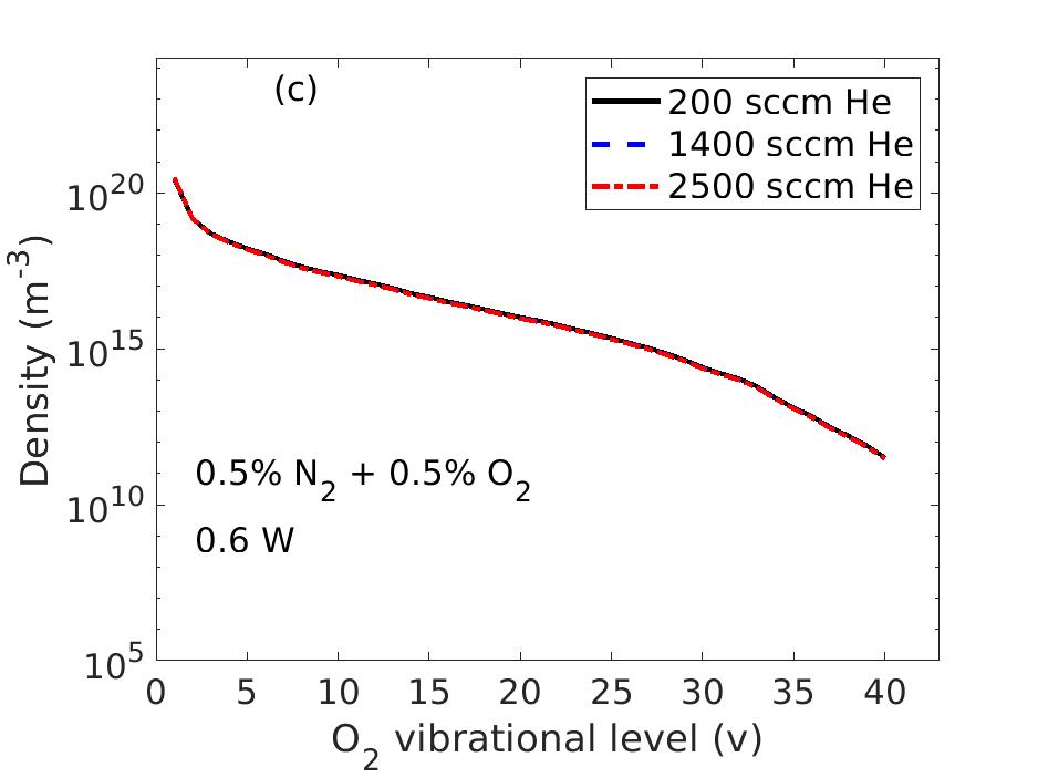
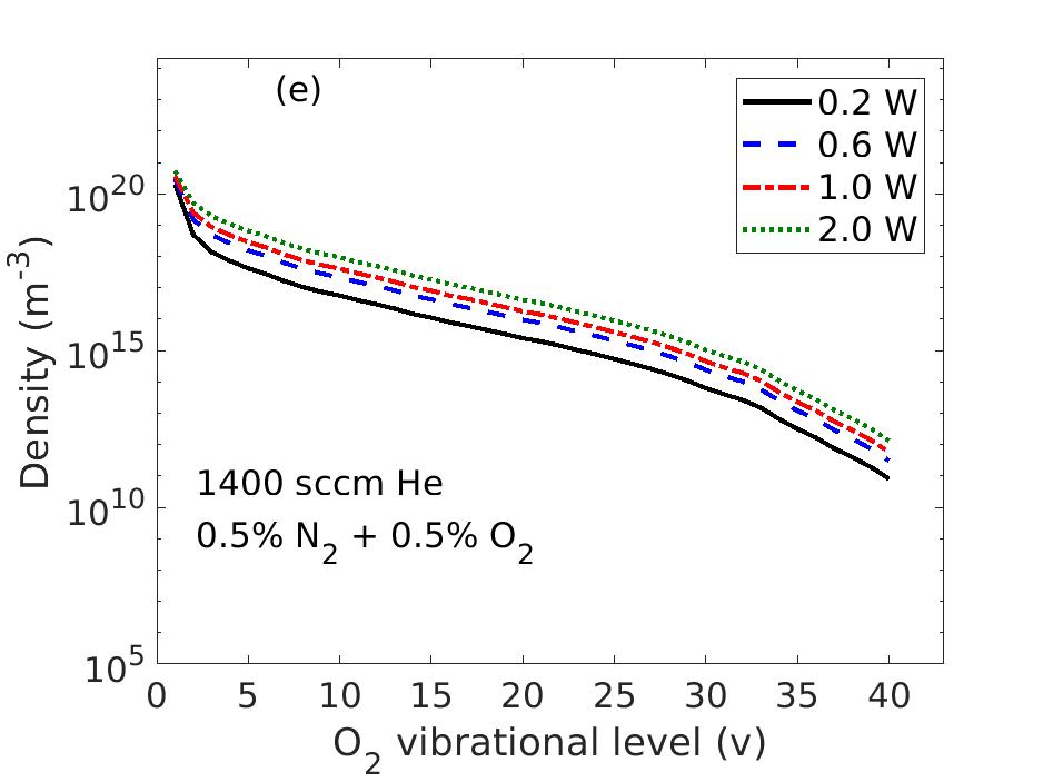
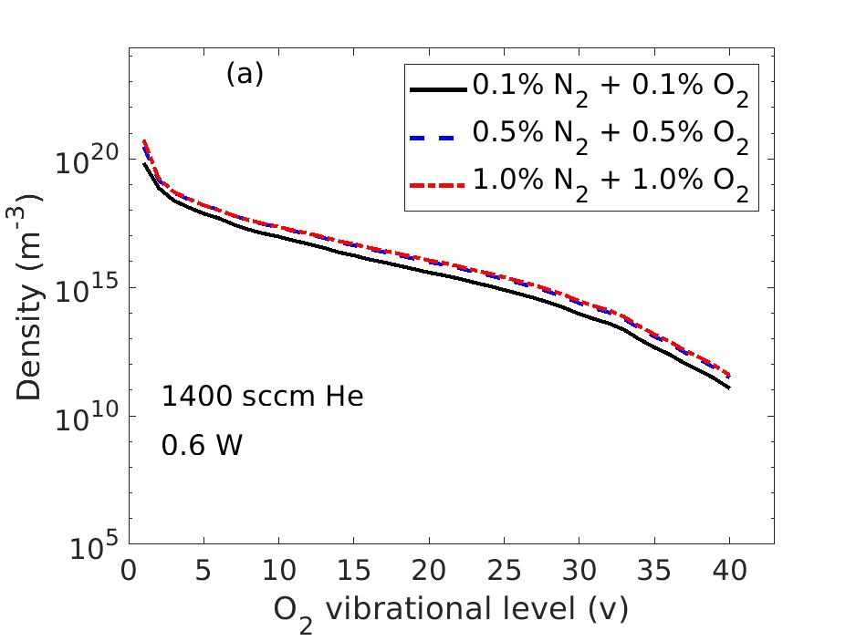
Figure 10: The zero-dimensional simulation results of the O2\mathrm{O_{2}} and N2\mathrm{N_{2}} VDFs in the COST-Jet for a variation of (a)−(b)(a)-(b) the mixture ratio (0.1 - 1.0 % N2\mathrm{N_{2}} + 0.1 - 1.0 % O2\mathrm{O_{2}}), (c)−(d)(c)-(d) the helium flow rate (200 - 2500 sccm) and (e)−(f)(e)-(f) the absorbed power (0.2 - 2.0 W) at a pressure of 101325 Pa and a gas temperature of 345 K.

The vibrational distribution functions in a He/N2\mathrm{N_{2}}/O2\mathrm{O_{2}} COST-Jet for a variation of the gas mixture ratio (0.1 - 1.0 % N2\mathrm{N_{2}} + 0.1 - 1.0 % O2\mathrm{O_{2}}), the helium flow rate (200 - 2500 sccm) and the absorbed power (0.2 - 2.0 W) are shown in figure 10. A close similarity is obtained between the distribution functions of the gas mixtures He/N2\mathrm{N_{2}}/O2\mathrm{O_{2}}, He/O2\mathrm{O_{2}} and He/N2\mathrm{N_{2}}, therefore only those of He/N2\mathrm{N_{2}}/O2\mathrm{O_{2}} are addressed here. Three distinct regions are located in the oxygen distribution function: (1) fast depletion at low, (2) plateau area at intermediate and (3) Boltzmann tail at high vibrational levels, similar to low-pressure oxygen plasma [33, 117]. The synergistic role of the whole vibrational chemical kinetics (i.e., e-V, V-V and V-T reactions) is important for the profile at low quantum numbers, whereas the V-T mechanism is more influential on the intermediate and high vibrational levels. A Maxwellian-like distribution function at low and intermediate vibrational quanta is obtained for nitrogen molecules, similar to those at low-pressure [118, 119, 30]. The tail of the distribution function is slightly elevated except at a high power of 2.02.0 W. The vibrational population is initially driven by e-V energy transfer, however the quasi-steady distribution function is mainly shaped by the V-V collisions. The negligible role of the electron-impact vibrational excitation at low quantum numbers is attributed to much higher densities of vibrationally excited nitrogen than that of electron. On the other hand, a more important influence of the e-V mechanisms on high quantum region is observed at lower absorbed power due to the significantly reduced vibrational population. Additionally, the increasing influence of the e-V mechanisms with decreasing power is the main mechanism responsible for the elevated tail at the low power operation (see figure 10(f)(f)).

The N2\mathrm{N_{2}} VDF shows a substantial dependency on the operation parameters relative to a weak response of the oxygen vibrational population. A likely reason is that the higher efficiency of nitrogen up-pumping promotes a larger variation with respect to the operation parameters. Furthermore, nitrogen levels store more internal energy with a reinforcement at higher quantum number. Hence, these levels are far more influential on the EEDF as well as on the resultant chemical kinetics [30]. For a high mixture ratio in figure 10(a)(a) and (b)(b), the collisions significantly re-distribute the vibrational energy stored in nitrogen and hence reduce the N2\mathrm{N_{2}} VDF. The re-distributed energy is partially transferred to a slightly enhanced oxygen vibrational population. The role of the gas flow rate in both oxygen and nitrogen vibrational populations in figure 10(c)(c) and (d)(d) is less important than those of the mixture ratio and the absorbed power due to the much less influence of the flow on the electron density and temperature. Both VDFs are enhanced with higher absorbed power shown in figure 10(e)(e) and (f)(f), as a result of the sufficient energy input to the e-V and V-V transfer for climbing the vibrational ladder.

Refer to caption
Refer to caption
Refer to caption
Refer to caption
Figure 11: The spatial evolution of the N2\mathrm{N_{2}} VDFs from entrance (0/4 L) to exit (4/4 L) of the plasma chamber. The COST-Jet is fed with 1400 sccm He + 0.5 % N2\mathrm{N_{2}} + 0.5 % O2\mathrm{O_{2}} at a pressure of 101325 Pa and a gas temperature of 345 K for absorbed powers of (a)(a) 0.2 W, (b)(b) 0.6 W, (c)(c) 1.0 W and (d)(d) 2.0 W.

The spatial evolution of the N2\mathrm{N_{2}} VDF in gas flow direction of the He/N2\mathrm{N_{2}}/O2\mathrm{O_{2}} COST-Jet is given in figure 11 for absorbed powers of (a)(a) 0.2 W, (b)(b) 0.6 W, (c)(c) 1.0 W and (d)(d) 2.0 W. The oxygen vibrational population is already saturated at one fourth of the plasma chamber length (1/4 L) and therefore it is not depicted in the figure. A significant growth of the N2\mathrm{N_{2}} VDF is observed in the direction of the flow. It is amplified with an increase of the absorbed power specifically at the tail region. The vibrational temperature Tv=1\mathrm{T_{v=1}} increases from 2097 K to 3358 K along the electrodes at an absorbed power of 0.2 W, whereas it raises from 6696 K to 16347 K at 2.0 W.

5.4 Sensitivity analyses

Refer to caption
Refer to caption
Figure 12: The variation of the simulated plasma properties at different resolution of VDFs relative to those at a detailed resolution with N(v<58)2{}_{2}(v<58) & O(v<41)2{}_{2}(v<41). The COST-Jet is sustained by an absorbed power of 0.60.6 W at a pressure of 101325101325 Pa and a gas temperature of 345345 K, and fed with (a)(a) 1400 sccm He + 0.5 % N2\mathrm{N_{2}} and (b)(b) 1400 sccm He + 0.5 % O2\mathrm{O_{2}} + 0.5 % N2\mathrm{N_{2}}.

The variation of the simulated COST-Jet plasma properties for varying numbers of vibrationally excited levels considered in the model is given in figure 12 relative to those including the whole set, N(v<58)2{}_{2}(v<58) & O(v<41)2{}_{2}(v<41). Those of the He/O2\mathrm{O_{2}} plasma jet are not shown here, since they are below 10 %. A virtually negligible deviation of the simulation results is observed between the cases of N(v<7)2{}_{2}(v<7) & O(v<7)2{}_{2}(v<7) and N(v<58)2{}_{2}(v<58) & O(v<41)2{}_{2}(v<41). However, the deviation substantially increases with a decreasing number of the vibrationally excited levels in the model. For a feeding gas mixture of He/N2\mathrm{N_{2}}, the densities of N2\mathrm{N_{2}}, N2​(A3​Σ)\mathrm{N_{2}(A^{3}\Sigma)} and N2​(B3​Π)\mathrm{N_{2}(B^{3}\Pi)} are altered significantly as shown in figure 12(a)(a). The electron and helium metastable densities as well as the electron temperature are varied up to about 35%35\>\% when the vibrational levels are completely ignored. The variation is remarkably larger for a feeding gas mixture of He/N2\mathrm{N_{2}}/O2\mathrm{O_{2}}, up to about 234%234\>\% presented in figure 12(b)(b). The plasma properties are strongly altered by an inclusion of N(v<4)2{}_{2}(v<4) & O(v<4)2{}_{2}(v<4), particularly on the densities of N2​(A3​Σ)\mathrm{N_{2}(A^{3}\Sigma)} and N2​(B3​Π)\mathrm{N_{2}(B^{3}\Pi)}. It should be emphasized that the quantitative analysis here is only valid for the considered operation conditions and the variation is reinforced with increasing absorbed power (not shown here).

Table 1: The variation of the simulated plasma properties for a wall reaction probability value of 1 relative to that of 0 is presented with a percentage of increase (“↑{\color[rgb]{0,0,1}\uparrow}”) or decrease (“↓{\color[rgb]{1,0,0}\downarrow}”). Those smaller than 1 % are set to 0 % for the sake of clarity. For the wall reactions labeled by a symbol “*” under “→{\color[rgb]{0,0,0}\rightarrow}”, the corresponding reactions are only included in this table for a sensitivity analysis, unless stated otherwise (see section 4 and table 12). The COST-Jet is sustained by an absorbed power of 0.60.6 W at a pressure of 101325101325 Pa and a gas temperature of 345345 K for a feeding gas mixture of 14001400 sccm He + 0.5 % O2\mathrm{O_{2}}, 14001400 sccm He + 0.5 % N2\mathrm{N_{2}} or 14001400 sccm He + 0.5 % N2\mathrm{N_{2}} + 0.5 % O2\mathrm{O_{2}}.
N(4S,2D)→w1/2N2\mathrm{N(^{4}S,\>^{2}D)}\xrightarrow[\text{}]{\text{w}}1/2\mathrm{N}_{2} O2​(a1​Δg)→wO2\mathrm{O_{2}(a^{1}\Delta_{g})}\xrightarrow[\text{}]{\text{w}}\mathrm{O}_{2} O(3P,1D)→*w1/2O2\mathrm{O(^{3}P,\>^{1}D)}\xrightarrow[{\color[rgb]{0,0.6,0}\textbf{*}}]{\text{w}}1/2\mathrm{O}_{2} O(3P)→*w1/3O3\mathrm{O(^{3}P)}\xrightarrow[{\color[rgb]{0,0.6,0}\textbf{*}}]{\text{w}}1/3\mathrm{O}_{3} N2​(v)→wN2​(v−1)\mathrm{N}_{2}(v)\xrightarrow[\text{}]{\text{w}}\mathrm{N}_{2}(v-1)
He/O2
O(3P)\mathrm{O(^{3}P)} −\;\;\;\;\;\;\;\;\;\;\;\;- ↓   3%\;\;\;\;\;\;\;\;{\color[rgb]{1,0,0}\downarrow}\;\>\>3\>\% ↓   58%\;\;\;\;\;\;\;\;{\color[rgb]{1,0,0}\downarrow}\;\>\>58\>\% ↓ 51%\;\;\;\;\;\;\;\;{\color[rgb]{1,0,0}\downarrow}\;51\>\% −\;\;\;\;\;\;\;\;\;\;\;\;-
O3\mathrm{O_{3}} −\;\;\;\;\;\;\;\;\;\;\;\;- ↑ 56%\;\;\;\;\;\;\;\;{\color[rgb]{0,0,1}\uparrow}\;56\>\% ↓   74%\;\;\;\;\;\;\;\;{\color[rgb]{1,0,0}\downarrow}\;\>\>74\>\% ↑ 16%\;\;\;\;\;\;\;\;{\color[rgb]{0,0,1}\uparrow}\;16\>\% −\;\;\;\;\;\;\;\;\;\;\;\;-
O(1D)\mathrm{O(^{1}D)} −\;\;\;\;\;\;\;\;\;\;\;\;- ↓   8%\;\;\;\;\;\;\;\;{\color[rgb]{1,0,0}\downarrow}\;\>\>8\>\% ↓   29%\;\;\;\;\;\;\;\;{\color[rgb]{1,0,0}\downarrow}\;\>\>29\>\% ↓   3%\;\;\;\;\;\;\;\;{\color[rgb]{1,0,0}\downarrow}\;\>\>3\>\% −\;\;\;\;\;\;\;\;\;\;\;\;-
O2​(a1​Δg)\mathrm{O_{2}(a^{1}\Delta_{g})} −\;\;\;\;\;\;\;\;\;\;\;\;- ↓ 44%\;\;\;\;\;\;\;\;{\color[rgb]{1,0,0}\downarrow}\;44\>\% ↑ 106%\;\;\;\;\;\;\;\;{\color[rgb]{0,0,1}\uparrow}\;106\>\% ↓ 10%\;\;\;\;\;\;\;\;{\color[rgb]{1,0,0}\downarrow}\;10\>\% −\;\;\;\;\;\;\;\;\;\;\;\;-
He/N2
N(4S)\mathrm{N(^{4}S)} ↓ 70%\;\;\;\;\;\;\;\;{\color[rgb]{1,0,0}\downarrow}\;70\>\% −\;\;\;\;\;\;\;\;\;\;\;\;- −\;\;\;\;\;\;\;\;\;\;\;\;- −\;\;\;\;\;\;\;\;\;\;\;\;- ↓ 13%\;\;\;\;\;\;\;\;{\color[rgb]{1,0,0}\downarrow}\;13\>\%
N(2D)\mathrm{N(^{2}D)} ↓ 50%\;\;\;\;\;\;\;\;{\color[rgb]{1,0,0}\downarrow}\;50\>\% −\;\;\;\;\;\;\;\;\;\;\;\;- −\;\;\;\;\;\;\;\;\;\;\;\;- −\;\;\;\;\;\;\;\;\;\;\;\;- ↓ 25%\;\;\;\;\;\;\;\;{\color[rgb]{1,0,0}\downarrow}\;25\>\%
N2​(v=3)\mathrm{N_{2}}(v=3)               0%\;\;\;\;\;\;\;\;\>\>\>\>\>\,0\>\% −\;\;\;\;\;\;\;\;\;\;\;\;- −\;\;\;\;\;\;\;\;\;\;\;\;- −\;\;\;\;\;\;\;\;\;\;\;\;- ↓ 32%\;\;\;\;\;\;\;\;{\color[rgb]{1,0,0}\downarrow}\;32\>\%
N2​(v=35)\mathrm{N_{2}}(v=35)               0%\;\;\;\;\;\;\;\;\>\>\>\>\>\,0\>\% −\;\;\;\;\;\;\;\;\;\;\;\;- −\;\;\;\;\;\;\;\;\;\;\;\;- −\;\;\;\;\;\;\;\;\;\;\;\;- ↓ 98%\;\;\;\;\;\;\;\;{\color[rgb]{1,0,0}\downarrow}\;98\>\%
He/N2/O2
N(4S)\mathrm{N(^{4}S)} ↓ 56%\;\;\;\;\;\;\;\;{\color[rgb]{1,0,0}\downarrow}\;56\>\% ↑   1%\;\;\;\;\;\;\;\;{\color[rgb]{0,0,1}\uparrow}\;\>\>1\>\% ↓     7%\;\;\;\;\;\;\;\;{\color[rgb]{1,0,0}\downarrow}\;\>\>\>\>7\>\% ↓   2%\;\;\;\;\;\;\;\;{\color[rgb]{1,0,0}\downarrow}\;\>\>2\>\% ↓ 47%\;\;\;\;\;\;\;\;{\color[rgb]{1,0,0}\downarrow}\;47\>\%
N(2D)\mathrm{N(^{2}D)} ↓   6%\;\;\;\;\;\;\;\;{\color[rgb]{1,0,0}\downarrow}\;\>\>6\>\% ↑   2%\;\;\;\;\;\;\;\;{\color[rgb]{0,0,1}\uparrow}\;\>\>2\>\% ↓     9%\;\;\;\;\;\;\;\;{\color[rgb]{1,0,0}\downarrow}\;\>\>\>\>9\>\% ↓   1%\;\;\;\;\;\;\;\;{\color[rgb]{1,0,0}\downarrow}\;\>\>1\>\% ↓ 28%\;\;\;\;\;\;\;\;{\color[rgb]{1,0,0}\downarrow}\;28\>\%
O(3P)\mathrm{O(^{3}P)}               0%\;\;\;\;\;\;\;\;\>\>\>\>\>\,0\>\% ↓   2%\;\;\;\;\;\;\;\;{\color[rgb]{1,0,0}\downarrow}\;\>\>2\>\% ↓   60%\;\;\;\;\;\;\;\;{\color[rgb]{1,0,0}\downarrow}\;\>\>60\>\% ↓ 53%\;\;\;\;\;\;\;\;{\color[rgb]{1,0,0}\downarrow}\;53\>\% ↓   1%\;\;\;\;\;\;\;\;{\color[rgb]{1,0,0}\downarrow}\;\>\>1\>\%
O3\mathrm{O_{3}}               0%\;\;\;\;\;\;\;\;\>\>\>\>\>\,0\>\% ↑ 35%\;\;\;\;\;\;\;\;{\color[rgb]{0,0,1}\uparrow}\;35\>\% ↓   75%\;\;\;\;\;\;\;\;{\color[rgb]{1,0,0}\downarrow}\;\>\>75\>\% ↑   3%\;\;\;\;\;\;\;\;{\color[rgb]{0,0,1}\uparrow}\;\>\>3\>\% ↑   1%\;\;\;\;\;\;\;\;{\color[rgb]{0,0,1}\uparrow}\;\>\>1\>\%
O(1D)\mathrm{O(^{1}D)}               0%\;\;\;\;\;\;\;\;\>\>\>\>\>\,0\>\% ↓   7%\;\;\;\;\;\;\;\;{\color[rgb]{1,0,0}\downarrow}\;\>\>7\>\% ↓   30%\;\;\;\;\;\;\;\;{\color[rgb]{1,0,0}\downarrow}\;\>\>30\>\% ↓   2%\;\;\;\;\;\;\;\;{\color[rgb]{1,0,0}\downarrow}\;\>\>2\>\% ↓   9%\;\;\;\;\;\;\;\;{\color[rgb]{1,0,0}\downarrow}\;\>\>9\>\%
O2​(a1​Δg)\mathrm{O_{2}(a^{1}\Delta_{g})}               0%\;\;\;\;\;\;\;\;\>\>\>\>\>\,0\>\% ↓ 36%\;\;\;\;\;\;\;\;{\color[rgb]{1,0,0}\downarrow}\;36\>\% ↑ 109%\;\;\;\;\;\;\;\;{\color[rgb]{0,0,1}\uparrow}\;109\>\% ↓   1%\;\;\;\;\;\;\;\;{\color[rgb]{1,0,0}\downarrow}\;\>\>1\>\% ↓   3%\;\;\;\;\;\;\;\;{\color[rgb]{1,0,0}\downarrow}\;\>\>3\>\%
NO\mathrm{NO} ↑   8%\;\;\;\;\;\;\;\;{\color[rgb]{0,0,1}\uparrow}\;\>\>8\>\% ↑   1%\;\;\;\;\;\;\;\;{\color[rgb]{0,0,1}\uparrow}\;\>\>1\>\% ↓   12%\;\;\;\;\;\;\;\;{\color[rgb]{1,0,0}\downarrow}\;\>\>12\>\% ↓   6%\;\;\;\;\;\;\;\;{\color[rgb]{1,0,0}\downarrow}\;\>\>6\>\% ↓ 46%\;\;\;\;\;\;\;\;{\color[rgb]{1,0,0}\downarrow}\;46\>\%
NO2\mathrm{NO_{2}} ↑   8%\;\;\;\;\;\;\;\;{\color[rgb]{0,0,1}\uparrow}\;\>\>8\>\% ↑   1%\;\;\;\;\;\;\;\;{\color[rgb]{0,0,1}\uparrow}\;\>\>1\>\% ↓   16%\;\;\;\;\;\;\;\;{\color[rgb]{1,0,0}\downarrow}\;\>\>16\>\% ↓   9%\;\;\;\;\;\;\;\;{\color[rgb]{1,0,0}\downarrow}\;\>\>9\>\% ↓ 45%\;\;\;\;\;\;\;\;{\color[rgb]{1,0,0}\downarrow}\;45\>\%
NO3\mathrm{NO_{3}} ↑   8%\;\;\;\;\;\;\;\;{\color[rgb]{0,0,1}\uparrow}\;\>\>8\>\% ↑   1%\;\;\;\;\;\;\;\;{\color[rgb]{0,0,1}\uparrow}\;\>\>1\>\% ↓   18%\;\;\;\;\;\;\;\;{\color[rgb]{1,0,0}\downarrow}\;\>\>18\>\% ↓ 11%\;\;\;\;\;\;\;\;{\color[rgb]{1,0,0}\downarrow}\;11\>\% ↓ 45%\;\;\;\;\;\;\;\;{\color[rgb]{1,0,0}\downarrow}\;45\>\%
N2​O3\mathrm{N_{2}O_{3}} ↑ 17%\;\;\;\;\;\;\;\;{\color[rgb]{0,0,1}\uparrow}\;17\>\% ↑   2%\;\;\;\;\;\;\;\;{\color[rgb]{0,0,1}\uparrow}\;\>\>2\>\% ↓   27%\;\;\;\;\;\;\;\;{\color[rgb]{1,0,0}\downarrow}\;\>\>27\>\% ↓ 16%\;\;\;\;\;\;\;\;{\color[rgb]{1,0,0}\downarrow}\;16\>\% ↓ 70%\;\;\;\;\;\;\;\;{\color[rgb]{1,0,0}\downarrow}\;70\>\%
N2​O4\mathrm{N_{2}O_{4}} ↑ 17%\;\;\;\;\;\;\;\;{\color[rgb]{0,0,1}\uparrow}\;17\>\% ↑   2%\;\;\;\;\;\;\;\;{\color[rgb]{0,0,1}\uparrow}\;\>\>2\>\% ↓   30%\;\;\;\;\;\;\;\;{\color[rgb]{1,0,0}\downarrow}\;\>\>30\>\% ↓ 18%\;\;\;\;\;\;\;\;{\color[rgb]{1,0,0}\downarrow}\;18\>\% ↓ 70%\;\;\;\;\;\;\;\;{\color[rgb]{1,0,0}\downarrow}\;70\>\%
N2​O5\mathrm{N_{2}O_{5}} ↑ 17%\;\;\;\;\;\;\;\;{\color[rgb]{0,0,1}\uparrow}\;17\>\% ↑   2%\;\;\;\;\;\;\;\;{\color[rgb]{0,0,1}\uparrow}\;\>\>2\>\% ↓   31%\;\;\;\;\;\;\;\;{\color[rgb]{1,0,0}\downarrow}\;\>\>31\>\% ↓ 19%\;\;\;\;\;\;\;\;{\color[rgb]{1,0,0}\downarrow}\;19\>\% ↓ 70%\;\;\;\;\;\;\;\;{\color[rgb]{1,0,0}\downarrow}\;70\>\%
N2​(v=3)\mathrm{N_{2}}(v=3)               0%\;\;\;\;\;\;\;\;\>\>\>\>\>\,0\>\%               0%\;\;\;\;\;\;\;\;\>\>\>\>\>\,0\>\% ↑     1%\;\;\;\;\;\;\;\;{\color[rgb]{0,0,1}\uparrow}\;\>\>\>\>1\>\%               0%\;\;\;\;\;\;\;\;\>\>\>\>\>\,0\>\% ↓ 36%\;\;\;\;\;\;\;\;{\color[rgb]{1,0,0}\downarrow}\;36\>\%
N2​(v=35)\mathrm{N_{2}}(v=35)               0%\;\;\;\;\;\;\;\;\>\>\>\>\>\,0\>\% ↓   4%\;\;\;\;\;\;\;\;{\color[rgb]{1,0,0}\downarrow}\;\>\>4\>\% ↑   11%\;\;\;\;\;\;\;\;{\color[rgb]{0,0,1}\uparrow}\;\>\>11\>\%               0%\;\;\;\;\;\;\;\;\>\>\>\>\>\,0\>\% ↓ 98%\;\;\;\;\;\;\;\;{\color[rgb]{1,0,0}\downarrow}\;98\>\%

The modification of the simulated plasma properties in the COST-Jet to the changes of the wall reaction probabilities from 0 to 1 is summarized in table 1 for the gas mixtures He/O2\mathrm{O_{2}}, He/N2\mathrm{N_{2}} and He/N2\mathrm{N_{2}}/O2\mathrm{O_{2}}. The COST-Jet He plasma is not altered by these changes and it is excluded from the table. The electron density and temperature are negligibly affected by the neutral wall reaction mechanisms within the considered gas mixtures. Additionally, it is observed that all the plasma properties are insensitive to the wall quenching of He⁡(23​S)\mathrm{He(2^{3}S)}, He2∗\mathrm{He_{2}^{*}}, N2​(A3​Σ)\mathrm{N_{2}(A^{3}\Sigma)}, N2​(B3​Π)\mathrm{N_{2}(B^{3}\Pi)}, O(1D)\mathrm{O(^{1}D)} and O2​(v<41)\mathrm{O_{2}}(v<41). The quenching of N(2D)\mathrm{N(^{2}D)} is of importance merely for its concentration in a He/N2\mathrm{N_{2}} jet (not shown here). In the He/O2 and He/N2\mathrm{N_{2}}/O2\mathrm{O_{2}} mixtures, an increase of the O2​(a1​Δg)\mathrm{O_{2}(a^{1}\Delta_{g})} quenching probability reduces the density of O2​(a1​Δg)\mathrm{O_{2}(a^{1}\Delta_{g})} and raises that of O3\mathrm{O_{3}}. The oxygen atom wall recombination and ozone wall formation probabilities have a significant influence on the O(3P)\mathrm{O(^{3}P)} density. Moreover, the recombination probability plays an important role in the concentrations of O3\mathrm{O_{3}} and O2​(a1​Δg)\mathrm{O_{2}(a^{1}\Delta_{g})}. In the He/N2\mathrm{N_{2}} and He/N2\mathrm{N_{2}}/O2\mathrm{O_{2}} mixtures, a rise of the nitrogen atom wall recombination probability reduces the densities of N(4S)\mathrm{N(^{4}S)} and N(2D)\mathrm{N(^{2}D)}. The wall quenching of N(v<58)2{}_{2}(v<58) has an impact on the vibrationally excited nitrogen molecule densities, particularly on those with high quantum numbers. This quenching additionally alters the concentrations of nitrogen atom and nitrogen oxides for a feeding gas mixture of He/N2\mathrm{N_{2}}/O2\mathrm{O_{2}}.

Refer to caption
Refer to caption
Refer to caption
Figure 13: The variation of the simulated plasma properties at varying orders of synthetic air impurity relative to those with a pure feeding gas. The COST-Jet is sustained by an absorbed power of 0.60.6 W at a pressure of 101325101325 Pa and a gas temperature of 345345 K for feeding gases of (a)(a) 1400 sccm He, (b)(b) 1400 sccm He + 0.5 % O2\mathrm{O_{2}} and (c)(c) 1400 sccm He + 0.5 % N2\mathrm{N_{2}}.

The variation of the simulated plasma properties at varying orders of synthetic air impurity relative to those with a pure feeding gas in the COST-Jet is shown in figure 13 for gases (a)(a) He, (b)(b) He/O2 and (c)(c) He/N2. The simulations confirm the substantial influence of the impurity level on the plasma properties. The electron density increases with increasing amount of synthetic air in He plasma, whereas the electron temperature as well as the densities of He⁡(23​S)\mathrm{He(2^{3}S)} and He2∗\mathrm{He_{2}^{*}} decrease. The metastable densities experience the largest variation due to the efficient Penning ionization by nitrogen and oxygen species [13]. The role of the synthetic air impurity in He/O2\mathrm{O_{2}} plasma is limited and produces below 10%10\>\% variation at a value of 100100 ppm. The He/N2\mathrm{N_{2}} mixture is comparatively more sensitive to this impurity level, and up to 60%60\>\% reduction of the concentrations is observed.

6 Conclusion

Atmospheric-pressure plasma jet devices of planar electrode configuration fed with He, He/O2\mathrm{O_{2}}, He/N2\mathrm{N_{2}} and He/N2\mathrm{N_{2}}/O2\mathrm{O_{2}} mixtures are investigated by a zero-dimensional (volume-averaged) and a pseudo-one-dimensional (plug-flow) modelling approach. The models are developed with a focus on the vibrational kinetics and self-consistently coupled with a Boltzmann solver (LoKI-B) under the two-term approximation to properly address the electron kinetics. A good agreement is obtained between the model calculations and the spatially resolved simulation results as well as diverse measurements available from literature, including the electron density, the electron temperature, and the concentrations of helium metastable, helium excimer, ozone, oxygen atom and nitrogen atom in distinct operation conditions.

Nitric oxide is thoroughly characterized for a variation of the gas mixture ratio, helium flow rate and absorbed power. The measurements at low power are better described by introducing the reactive quenching of N2​(A3​Σ,B3​Π,v>0)\mathrm{N_{2}(A^{3}\Sigma,B^{3}\Pi;}\>v>0) and of multiple N2\mathrm{N_{2}} electronically excited states with a hypothetical `​```effective"" rate coefficient value in the simulations, that forms underlying NO production mechanisms as well as significant O(3P)\mathrm{O(^{3}P)} loss channels. A continuous growth of the NO spatial density profile is obtained in gas flow direction, and the saturation is merely observed at a relatively high absorbed power of about 2.2 W. Within the range of the considered operation conditions, the NO loss is governed by its flow-out rate, the O(3P)+NO+M→NO2+M\mathrm{O(^{3}P)}+\mathrm{NO}+\mathrm{M}\rightarrow\mathrm{NO_{2}}+\mathrm{M} and N(4S)+NO→N2+O(3P)\mathrm{N(^{4}S)}+\mathrm{NO}\rightarrow\mathrm{N_{2}}+\mathrm{O(^{3}P)} reactions, while the formation is dominated by the O(3P)+NO2→NO+O2\mathrm{O(^{3}P)}+\mathrm{NO_{2}}\rightarrow\mathrm{NO}+\mathrm{O_{2}} and N(2D)+O2→NO+O(1D)\mathrm{N(^{2}D)}+\mathrm{O_{2}}\rightarrow\mathrm{NO}+\mathrm{O(^{1}D)} channels. The contribution of the vibrationally excited nitrogen molecules N2​(v⩾13)\mathrm{N_{2}}(v\geqslant 13) in the net NO formation is enhanced with increasing power.

The vibrationally excited levels of O2​(v<41)\mathrm{O_{2}}(v<41) and N2​(v<58)\mathrm{N_{2}}(v<58) are analysed. A larger response of the N2 VDF to the variation of the gas mixture ratio, helium flow rate and absorbed power is observed relative to that of the O2 VDF. A continuous spatial growth of the N2 vibrational population is obtained in gas flow direction (i.e., the population is not yet saturated at the jet nozzle). On the contrary, a fast spatial equilibrium of the O2 vibrational population is acquired at the beginning of the plasma chamber. The simulation results are affected by the total number of vibrationally excited nitrogen molecules considered in the chemical model. However, the influence of N2​(v<58)\mathrm{N_{2}}(v<58) on the overall plasma behaviour is captured by a limited set of vibrational levels depending on the applied power value.

The sensitivity of the simulation results to a variation of the wall reaction probabilities and the synthetic air impurity levels is provided. The concentrations of nitrogen atom and nitrogen oxides are influenced by the wall quenching of vibrationally excited nitrogen molecules. A dramatic sensitivity of the atomic oxygen and ozone densities to the oxygen atom wall recombination is observed. The plasma properties of pure He gas are significantly altered in the presence of the impurity due to the efficient Penning ionization mechanism. An impurity level up to 100 ppm is not influential on the simulation results of He/O2\mathrm{O_{2}} mixture, but has a strong impact on those of He/N2\mathrm{N_{2}} plasma.

A further analysis of the rate coefficients of the termolecular Penning ionization He⁡(23​S)+N2+He→e+N2++2​He\mathrm{He(2^{3}S)}+\mathrm{N_{2}}+\mathrm{He}\rightarrow e+\mathrm{N_{2}^{+}}+2\mathrm{He}, the metastable quenching via vibrationally excited nitrogen molecules He⁡(23​S)+N2​(v>0)→e+He+N2+{\rm He(2^{3}S)}+{\rm N}_{2}(v>0)\rightarrow e+{\rm He}+{\rm N}_{2}^{+} and the nitric oxide formation channels N2(X,A3Σ,B3Π,…;v)+O(3P)→NO+N(2D)\mathrm{N_{2}(X,A^{3}\Sigma,B^{3}\Pi,...;}\>v)+{\rm O(^{3}P)}\rightarrow{\rm NO}+{\rm N(^{2}D)} is of importance for a more accurate model prediction.

Acknowledgements

Funded by the Deutsche Forschungsgemeinschaft (DFG, German Research Foundation) - Project-ID 327886311 (SFB 1316: simulations by A9 & A8 and measurements by B2 & A4). The authors are in depth with Antonio Tejero del Caz and Luis L. Alves for discussions on the self-consistent LoKI-B adaptation, with Peter Bruggeman and Nader Sadeghi for discussions on the pulse-modulated plasma jet, and with Judith Golda for discussions on the experimental details of the He COST-Jet. Vasco Guerra was partially funded by the Portuguese FCT-Fundacao para a Ciencia e a Tecnologia, under projects UIDB/50010/2020 and UIDP/50010/2020.

ORCID iDs

Volker Schulz-von der Gathen https://orcid.org/0000-0002-7182-3253

Appendix

Appendix A Chemical kinetics

Table 2: The distinct species in the model of He\mathrm{He}, He/O2\mathrm{He/O_{2}}, He/N2\mathrm{He/N_{2}} or He/N2/O2\mathrm{He/N_{2}/O_{2}} are selected from the table below.
Plasma species
He\mathrm{He}, He⁡(23​S)\mathrm{He(2^{3}S)}, He2∗\mathrm{He_{2}^{*}}, He+\mathrm{He^{+}}, He2+\mathrm{He_{2}^{+}},
N(4S)\mathrm{N(^{4}S)}, N2\mathrm{N_{2}}, N(2D)\mathrm{N(^{2}D)}, N2​(A3​Σ)\mathrm{N_{2}(A^{3}\Sigma)}, N2​(B3​Π)\mathrm{N_{2}(B^{3}\Pi)}, N+\mathrm{N^{+}}, N2+\mathrm{N_{2}^{+}}, N3+\mathrm{N_{3}^{+}}, N4+\mathrm{N_{4}^{+}},
O(3P)\mathrm{O(^{3}P)}, O2\mathrm{O_{2}}, O3\mathrm{O_{3}}, O(1D)\mathrm{O(^{1}D)}, O2​(a1​Δg)\mathrm{O_{2}(a^{1}\Delta_{g})}, O+\mathrm{O^{+}}, O2+\mathrm{O_{2}^{+}}, O4+\mathrm{O_{4}^{+}}, O−\mathrm{O^{-}}, O2−\mathrm{O_{2}^{-}}, O3−\mathrm{O_{3}^{-}}, O4−\mathrm{O_{4}^{-}},
NO\mathrm{NO}, NO2\mathrm{NO_{2}}, NO3\mathrm{NO_{3}}, N2​O\mathrm{N_{2}O}, N2​O3\mathrm{N_{2}O_{3}}, N2​O4\mathrm{N_{2}O_{4}}, N2​O5\mathrm{N_{2}O_{5}}, NO+\mathrm{NO^{+}}, NO2+\mathrm{NO_{2}^{+}}, N2​O+\mathrm{N_{2}O^{+}}, NO−\mathrm{NO^{-}}, NO2−\mathrm{NO_{2}^{-}}, NO3−\mathrm{NO_{3}^{-}}, N2​O−\mathrm{N_{2}O^{-}},
N2\mathrm{N_{2}}(0<v<<v<58), O2\mathrm{O_{2}}(0<v<<v<41), ee
Table 3: The volume reactions included in the He\mathrm{He} model. The rate coefficient units are given in s-1, m3 s-1 and m6 s-1 for one-, two- and three-body reactions, respectively. Te\rm T_{e} is in eV and Tg\rm T_{g} in K, if not stated otherwise. The rate coefficient f⁡(ϵ)f(\epsilon) is taken from a look-up-table calculated via the referred cross-section self-consistently coupled to the EEDF [56]. The reverse reaction rate coefficient of the electron-impact excitation labeled with a symbol “*” near the number is calculated via the principle of detailed balancing [64].
# Reaction Rate Coefficient Ref
1 e+He→2​e+He+e+\mathrm{He}\rightarrow 2e+\mathrm{He^{+}} f⁡(ϵ)f(\epsilon) [85]
2∗ e+He→e+He⁡(23​S)e+\mathrm{He}\rightarrow e+\mathrm{He(2^{3}S)} f⁡(ϵ)f(\epsilon) [85]
3 e+He⁡(23​S)→2​e+He+e+\mathrm{He(2^{3}S)}\rightarrow 2e+\mathrm{He^{+}} f⁡(ϵ)f(\epsilon) [120]
4 e+He2∗→e+2​Hee+\mathrm{He_{2}^{*}}\rightarrow e+2\mathrm{He} 3.8×10−153.8\times 10^{-15} [16]
5 e+He2∗→2​e+He2+e+\mathrm{He_{2}^{*}}\rightarrow 2e+\mathrm{He_{2}^{+}} f⁡(ϵ)f(\epsilon) [121]
6 e+He+→He⁡(23​S)e+\mathrm{He^{+}}\rightarrow\mathrm{He(2^{3}S)} 5.95×10⁻¹⁷T[K]−0.5e5.95\times 10^{-17}\>T{\rm{}_{e}[K]}^{-0.5} [14]
7 2​e+He+→e+He⁡(23​S)2e+\mathrm{He^{+}}\rightarrow e+\mathrm{He(2^{3}S)} 1.63×10⁻²¹T[K]−4.5e1.63\times 10^{-21}\>T{\rm{}_{e}[K]}^{-4.5} [14]
8 e+He++He→He⁡(23​S)+Hee+\mathrm{He^{+}}+\mathrm{He}\rightarrow\mathrm{He(2^{3}S)}+\mathrm{He} 7.4×10−47​(Te/Tg)−27.4\times 10^{-47}\>(T_{\rm e}/T_{\rm g})^{-2} [122]
9 e+He2+→He+Hee+\mathrm{He_{2}^{+}}\rightarrow\mathrm{He}+\mathrm{He} 1.0×10−151.0\times 10^{-15} [122]
10 e+He2+→He⁡(23​S)+Hee+\mathrm{He_{2}^{+}}\rightarrow\mathrm{He(2^{3}S)}+\mathrm{He} 8.9×10⁻¹⁵(Tg/T[K]e)−1.58.9\times 10^{-15}\>(T_{\rm g}/T{\rm{}_{e}[K]})^{-1.5} [123]
11 He++2​He→He2++He\mathrm{He^{+}}+2\mathrm{He}\rightarrow\mathrm{He_{2}^{+}}+\mathrm{He} 1.1×10−431.1\times 10^{-43} [123]
12 He⁡(23​S)+2​He→He2∗+He\mathrm{He(2^{3}S)}+2\mathrm{He}\rightarrow\mathrm{He_{2}^{*}}+\mathrm{He} 2×10−462\times 10^{-46} [123]
13 He⁡(23​S)+2​He→3​He\mathrm{He(2^{3}S)}+2\mathrm{He}\rightarrow 3\mathrm{He} 2×10−462\times 10^{-46} [122]
14 He⁡(23​S)+He⁡(23​S)→e+He2+\mathrm{He(2^{3}S)}+\mathrm{He(2^{3}S)}\rightarrow e+\mathrm{He_{2}^{+}} 1.5×10−151.5\times 10^{-15} [123]
15 He⁡(23​S)+He⁡(23​S)→e+He++He\mathrm{He(2^{3}S)}+\mathrm{He(2^{3}S)}\rightarrow e+\mathrm{He^{+}}+\mathrm{He} 8.7×10⁻¹⁶​(Tg/300)0.58.7\times 10^{-16}\>(T_{\rm g}/300)^{0.5} [122]
16 He⁡(23​S)+He2∗→e+He2++He\mathrm{He(2^{3}S)}+\mathrm{He_{2}^{*}}\rightarrow e+\mathrm{He_{2}^{+}}+\mathrm{He} 2.0×10−152.0\times 10^{-15} [122]
17 He⁡(23​S)+He2∗→e+He++2​He\mathrm{He(2^{3}S)}+\mathrm{He_{2}^{*}}\rightarrow e+\mathrm{He^{+}}+2\mathrm{He} 5.0×10−165.0\times 10^{-16} [122]
18 He2∗→2​He\mathrm{He_{2}^{*}}\rightarrow 2\mathrm{He} 1×1041\times 10^{4} [124]
19 He2∗+He→3​He\mathrm{He_{2}^{*}}+\mathrm{He}\rightarrow 3\mathrm{He} 1.5×10−211.5\times 10^{-21} [122]
20 He2∗+He2∗→e+He2++2​He\mathrm{He_{2}^{*}}+\mathrm{He_{2}^{*}}\rightarrow e+\mathrm{He_{2}^{+}}+2\mathrm{He} 1.5×10−151.5\times 10^{-15} [123]
21 He2∗+He2∗→e+He++3​He\mathrm{He_{2}^{*}}+\mathrm{He_{2}^{*}}\rightarrow e+\mathrm{He^{+}}+3\mathrm{He} 3.0×10−163.0\times 10^{-16} [122]
Table 4: The oxygen volume reactions in the He/O2\mathrm{He/O_{2}} model. M is the background gas helium. The rate coefficient units are given in m3 s-1 and m6 s-1 for two- and three-body reactions, respectively. Te\rm T_{e} is in eV and Tg\rm T_{g} in K, if not stated otherwise. The rate coefficient f⁡(ϵ)f(\epsilon) is taken from a look-up-table calculated via the referred cross-section self-consistently coupled to the EEDF [56]. The reverse reaction rate coefficients of the electron-impact excitation labeled with a symbol “*” near the number are calculated via the principle of detailed balancing [64].
# Reaction Rate Coefficient Ref
1 e+O(3P)+O2→O−+O2e+\mathrm{O(^{3}P)}+\mathrm{O_{2}}\rightarrow\mathrm{O^{-}}+\mathrm{O_{2}} 1×10−431\times 10^{-43} [82]
2 e+O(3P)+O2→O2−+O(3P)e+\mathrm{O(^{3}P)}+\mathrm{O_{2}}\rightarrow\mathrm{O_{2}^{-}}+\mathrm{O(^{3}P)} 1×10−431\times 10^{-43} [82]
3∗ e+O(3P)→e+O(1D)e+\mathrm{O(^{3}P)}\rightarrow e+\mathrm{O(^{1}D)} f⁡(ϵ)f(\epsilon) [85]
4 e+O(3P)→2e+O+e+\mathrm{O(^{3}P)}\rightarrow 2e+\mathrm{O^{+}} f⁡(ϵ)f(\epsilon) [85]
5 e+O2→O2−e+\mathrm{O_{2}}\rightarrow\mathrm{O_{2}^{-}} f⁡(ϵ)f(\epsilon) [125]
6 e+O2+O2→O2−+O2e+\mathrm{O_{2}}+\mathrm{O_{2}}\rightarrow\mathrm{O_{2}^{-}}+\mathrm{O_{2}} 1.4×10−41(Tg/T[K]e)exp(−600/Tg)×exp{700(T[K]e−Tg)/(T[K]eTg)}1.4\times 10^{-41}\>(T_{\rm g}/T{\rm{}_{e}[K]})\>{\rm exp}(-600/T_{\rm g})\times{\rm exp}\{700(T{\rm{}_{e}[K]}-T_{\rm g})/(T{\rm{}_{e}[K]}T_{\rm g})\} [126]
7 e+O2+He→He+O2−e+\mathrm{O_{2}}+\mathrm{He}\rightarrow\mathrm{He}+\mathrm{O_{2}^{-}} 8.8×10−42T[K]−0.5e8.8\times 10^{-42}\>T{\rm{}_{e}[K]}^{-0.5} [14]
8 e+O2→O−+O(3P)e+\mathrm{O_{2}}\rightarrow\mathrm{O^{-}}+\mathrm{O(^{3}P)} f⁡(ϵ)f(\epsilon) [85]
9 e+O2→e+2O(3P)e+\mathrm{O_{2}}\rightarrow e+2\mathrm{O(^{3}P)} f⁡(ϵ)f(\epsilon) [85]
10 e+O2→e+O(1D)+O(3P)e+\mathrm{O_{2}}\rightarrow e+\mathrm{O(^{1}D)}+\mathrm{O(^{3}P)} f⁡(ϵ)f(\epsilon) [85]
11 e+O2→2e+O++O(3P)e+\mathrm{O_{2}}\rightarrow 2e+\mathrm{O^{+}}+\mathrm{O(^{3}P)} f⁡(ϵ)f(\epsilon) [120]
12∗ e+O2→e+O2​(a1​Δg)e+\mathrm{O_{2}}\rightarrow e+\mathrm{O_{2}(a^{1}\Delta_{g})} f⁡(ϵ)f(\epsilon) [85]
13 e+O2→2​e+O2+e+\mathrm{O_{2}}\rightarrow 2e+\mathrm{O_{2}^{+}} f⁡(ϵ)f(\epsilon) [85]
14 e+O3+M→O3−+Me+\mathrm{O_{3}}+\mathrm{M}\rightarrow\mathrm{O_{3}^{-}}+\mathrm{M} 1×10−431\times 10^{-43} [82]
15 e+O3→O−+O2e+\mathrm{O_{3}}\rightarrow\mathrm{O^{-}}+\mathrm{O_{2}} f⁡(ϵ)f(\epsilon) [127]
16 e+O3→O(3P)+O2−e+\mathrm{O_{3}}\rightarrow\mathrm{O(^{3}P)}+\mathrm{O_{2}^{-}} f⁡(ϵ)f(\epsilon) [127]
17 e+O3→e+O(3P)+O2e+\mathrm{O_{3}}\rightarrow e+\mathrm{O(^{3}P)}+\mathrm{O_{2}} 8.8×10−168.8\times 10^{-16} [128]
18 e+O(1D)→2e+O+e+\mathrm{O(^{1}D)}\rightarrow 2e+\mathrm{O^{+}} f⁡(ϵ)f(\epsilon) [129]
19 e+O2(a1Δg)→O(3P)+O−e+\mathrm{O_{2}(a^{1}\Delta_{g})}\rightarrow\mathrm{O(^{3}P)}+\mathrm{O^{-}} f⁡(ϵ)f(\epsilon) [120]
20 e+O2(a1Δg)→e+2O(3P)e+\mathrm{O_{2}(a^{1}\Delta_{g})}\rightarrow e+2\mathrm{O(^{3}P)} f⁡(ϵ)f(\epsilon) [120]
21 e+O2(a1Δg)→e+O(3P)+O(1D)e+\mathrm{O_{2}(a^{1}\Delta_{g})}\rightarrow e+\mathrm{O(^{3}P)}+\mathrm{O(^{1}D)} f⁡(ϵ)f(\epsilon) [120]
22 e+O2(a1Δg)→2e+O(3P)+O+e+\mathrm{O_{2}(a^{1}\Delta_{g})}\rightarrow 2e+\mathrm{O(^{3}P)}+\mathrm{O^{+}} f⁡(ϵ)f(\epsilon) [120]
23 e+O2​(a1​Δg)→2​e+O2+e+\mathrm{O_{2}(a^{1}\Delta_{g})}\rightarrow 2e+\mathrm{O_{2}^{+}} f⁡(ϵ)f(\epsilon) [120]
24 e+e+O+→e+O(3P)e+e+\mathrm{O^{+}}\rightarrow e+\mathrm{O(^{3}P)} 1×10⁻³¹(Tg/T[K]e)4.51\times 10^{-31}\>(T_{\rm g}/T{\rm{}_{e}[K]})^{4.5} [81]
25 e+O++M→O(3P)+Me+\mathrm{O^{+}}+\mathrm{M}\rightarrow\mathrm{O(^{3}P)}+\mathrm{M} 3.12×10⁻³⁵/T[K]1.5e3.12\times 10^{-35}\>/T{\rm{}_{e}[K]}^{1.5} [81]
26 e+O+→O(1D)e+\mathrm{O^{+}}\rightarrow\mathrm{O(^{1}D)} 4.66×10⁻¹⁷T[K]−0.5e4.66\times 10^{-17}\>T{\rm{}_{e}[K]}^{-0.5} [14]
27 2e+O+→e+O(1D)2e+\mathrm{O^{+}}\rightarrow e+\mathrm{O(^{1}D)} 1.628×10⁻²¹T[K]−4.5e1.628\times 10^{-21}\>T{\rm{}_{e}[K]}^{-4.5} [14]
28 e+O2++M→O2+Me+\mathrm{O_{2}^{+}}+\mathrm{M}\rightarrow\mathrm{O_{2}}+\mathrm{M} 3.12×10⁻³⁵/T[K]1.5e3.12\times 10^{-35}\>/T{\rm{}_{e}[K]}^{1.5} [81]
29 e+e+O2+→e+O2e+e+\mathrm{O_{2}^{+}}\rightarrow e+\mathrm{O_{2}} 1×10⁻³¹(Tg/T[K]e)4.51\times 10^{-31}\>(T_{\rm g}/T{\rm{}_{e}[K]})^{4.5} [81]
30 e+O2+→2O(3P)e+\mathrm{O_{2}^{+}}\rightarrow 2\mathrm{O(^{3}P)} f⁡(ϵ)f(\epsilon) [130]
31 e+O2+→O(1D)+O(3P)e+\mathrm{O_{2}^{+}}\rightarrow\mathrm{O(^{1}D)}+\mathrm{O(^{3}P)} 4.688×10⁻¹²T[K]−0.7e4.688\times 10^{-12}\>T{\rm{}_{e}[K]}^{-0.7} [14]
32 e+O4+→O2+O2e+\mathrm{O_{4}^{+}}\rightarrow\mathrm{O_{2}}+\mathrm{O_{2}} 2.42×10⁻¹¹/T[K]0.5e2.42\times 10^{-11}\>/T{\rm{}_{e}[K]}^{0.5} [82]
33 e+O−→2e+O(3P)e+\mathrm{O^{-}}\rightarrow 2e+\mathrm{O(^{3}P)} 2.2×10⁻²⁰T[K]0.5eexp(−26356/T[K]e)2.2\times 10^{-20}\>T{\rm{}_{e}[K]}^{0.5}\>{\rm exp}(-26356/T{\rm{}_{e}[K]}) [14]
34 He+He++O−→2He+O(3P)\mathrm{He}+\mathrm{He^{+}}+\mathrm{O^{-}}\rightarrow 2\mathrm{He}+\mathrm{O(^{3}P)} 2×10−37​(300/Tg)2.52\times 10^{-37}\>(300/T_{\rm g})^{2.5} [14]
35 He+O(3P)+O+→He+O2+\mathrm{He}+\mathrm{O(^{3}P)}+\mathrm{O^{+}}\rightarrow\mathrm{He}+\mathrm{O_{2}^{+}} 1×10−41​(300/Tg)−0.51\times 10^{-41}\>(300/T_{\rm g})^{-0.5} [14]
36 He+O−+O+→He+2O(3P)\mathrm{He}+\mathrm{O^{-}}+\mathrm{O^{+}}\rightarrow\mathrm{He}+2\mathrm{O(^{3}P)} 2×10−37​(300/Tg)2.52\times 10^{-37}\>(300/T_{\rm g})^{2.5} [14]
37 He+O−+O2+→He+O(3P)+O2\mathrm{He}+\mathrm{O^{-}}+\mathrm{O_{2}^{+}}\rightarrow\mathrm{He}+\mathrm{O(^{3}P)}+\mathrm{O_{2}} 2×10−37​(300/Tg)2.52\times 10^{-37}\>(300/T_{\rm g})^{2.5} [14]
38 He++O(3P)→He+O+\mathrm{He^{+}}+\mathrm{O(^{3}P)}\rightarrow\mathrm{He}+\mathrm{O^{+}} 5×10⁻¹⁷​(300/Tg)−0.55\times 10^{-17}\>(300/T_{\rm g})^{-0.5} [14]
39 He++O2→He+O(3P)+O+\mathrm{He^{+}}+\mathrm{O_{2}}\rightarrow\mathrm{He}+\mathrm{O(^{3}P)}+\mathrm{O^{+}} 1.07×10⁻¹⁵​(300/Tg)−0.51.07\times 10^{-15}\>(300/T_{\rm g})^{-0.5} [14]
40 He++O2→He+O2+\mathrm{He^{+}}+\mathrm{O_{2}}\rightarrow\mathrm{He}+\mathrm{O_{2}^{+}} 3.3×10⁻¹⁷​(300/Tg)−0.53.3\times 10^{-17}\>(300/T_{\rm g})^{-0.5} [14]
41 He++O3→He+O++O2\mathrm{He^{+}}+\mathrm{O_{3}}\rightarrow\mathrm{He}+\mathrm{O^{+}}+\mathrm{O_{2}} 1.07×10⁻¹⁵​(300/Tg)−0.51.07\times 10^{-15}\>(300/T_{\rm g})^{-0.5} [14]
42 He++O(1D)→He+O+\mathrm{He^{+}}+\mathrm{O(^{1}D)}\rightarrow\mathrm{He}+\mathrm{O^{+}} 5×10⁻¹⁷​(300/Tg)−0.55\times 10^{-17}\>(300/T_{\rm g})^{-0.5} [14]
43 He++O2(a1Δg)→He+O(3P)+O+\mathrm{He^{+}}+\mathrm{O_{2}(a^{1}\Delta_{g})}\rightarrow\mathrm{He}+\mathrm{O(^{3}P)}+\mathrm{O^{+}} 1.07×10⁻¹⁵​(300/Tg)−0.51.07\times 10^{-15}\>(300/T_{\rm g})^{-0.5} [14]
44 He++O2​(a1​Δg)→He+O2+\mathrm{He^{+}}+\mathrm{O_{2}(a^{1}\Delta_{g})}\rightarrow\mathrm{He}+\mathrm{O_{2}^{+}} 3.3×10⁻¹⁷​(300/Tg)−0.53.3\times 10^{-17}\>(300/T_{\rm g})^{-0.5} [14]
45 O++O(3P)+O2→O2+O2+\mathrm{O^{+}}+\mathrm{O(^{3}P)}+\mathrm{O_{2}}\rightarrow\mathrm{O_{2}}+\mathrm{O_{2}^{+}} 1×10−42​(300/Tg)−0.51\times 10^{-42}\>(300/T_{\rm g})^{-0.5} [14]
46 O++O2→O(3P)+O2+\mathrm{O^{+}}+\mathrm{O_{2}}\rightarrow\mathrm{O(^{3}P)}+\mathrm{O_{2}^{+}} 2×10⁻¹⁷​(300/Tg)0.42\times 10^{-17}\>(300/T_{\rm g})^{0.4} [14]
47 O++O3→O2+O2+\mathrm{O^{+}}+\mathrm{O_{3}}\rightarrow\mathrm{O_{2}}+\mathrm{O_{2}^{+}} 1×10−161\times 10^{-16} [14]
48 O2++O2+M→O4++M\mathrm{O_{2}^{+}}+\mathrm{O_{2}}+\mathrm{M}\rightarrow\mathrm{O_{4}^{+}}+\mathrm{M} 5.5×10−43​(300/Tg)2.75.5\times 10^{-43}\>(300/T_{\rm g})^{2.7} [131]
49 O4++O(3P)→O2++O3\mathrm{O_{4}^{+}}+\mathrm{O(^{3}P)}\rightarrow\mathrm{O_{2}^{+}}+\mathrm{O_{3}} 3×10−163\times 10^{-16} [81]
50 O4++O2→O2++O2+O2\mathrm{O_{4}^{+}}+\mathrm{O_{2}}\rightarrow\mathrm{O_{2}^{+}}+\mathrm{O_{2}}+\mathrm{O_{2}} 3.3×10⁻¹²(300/Tg)4exp(−5030/Tg)3.3\times 10^{-12}\>(300/T_{\rm g})^{4}\>{\rm exp}(-5030/T_{\rm g}) [81]
51 O−+O(3P)→e+O2\mathrm{O^{-}}+\mathrm{O(^{3}P)}\rightarrow e+\mathrm{O_{2}} 2×10⁻¹⁶​(300/Tg)−0.52\times 10^{-16}\>(300/T_{\rm g})^{-0.5} [14]
52 O2−+O2→O2+O2+e\mathrm{O_{2}^{-}}+\mathrm{O_{2}}\rightarrow\mathrm{O_{2}}+\mathrm{O_{2}}+e 2.7×10⁻¹⁶(Tg/300)0.5exp(−5590/Tg)2.7\times 10^{-16}\>(T_{\rm g}/300)^{0.5}\>{\rm exp}(-5590/T_{\rm g}) [82]
53 O−+O2→e+O3\mathrm{O^{-}}+\mathrm{O_{2}}\rightarrow e+\mathrm{O_{3}} 5×10⁻¹⁸​(300/Tg)−0.55\times 10^{-18}\>(300/T_{\rm g})^{-0.5} [14]
54 O−+O2+M→O3−+M\mathrm{O^{-}}+\mathrm{O_{2}}+\mathrm{M}\rightarrow\mathrm{O_{3}^{-}}+\mathrm{M} 1.1×10−42​(300/Tg)1.1\times 10^{-42}\>(300/T_{\rm g}) [82]
55 O−+O2+O+→2O(3P)+O2\mathrm{O^{-}}+\mathrm{O_{2}}+\mathrm{O^{+}}\rightarrow 2\mathrm{O(^{3}P)}+\mathrm{O_{2}} 2×10−37​(300/Tg)2.52\times 10^{-37}\>(300/T_{\rm g})^{2.5} [14]
56 O−+O2+O2+→O(3P)+2O2\mathrm{O^{-}}+\mathrm{O_{2}}+\mathrm{O_{2}^{+}}\rightarrow\mathrm{O(^{3}P)}+2\mathrm{O_{2}} 2×10−37​(300/Tg)2.52\times 10^{-37}\>(300/T_{\rm g})^{2.5} [14]
57 O−+O2+O2+→O2+O3\mathrm{O^{-}}+\mathrm{O_{2}}+\mathrm{O_{2}^{+}}\rightarrow\mathrm{O_{2}}+\mathrm{O_{3}} 2×10−37​(300/Tg)2.52\times 10^{-37}\>(300/T_{\rm g})^{2.5} [64]
58 O−+O3→e+2​O2\mathrm{O^{-}}+\mathrm{O_{3}}\rightarrow e+2\mathrm{O_{2}} 3.01×10⁻¹⁶​(300/Tg)−0.53.01\times 10^{-16}\>(300/T_{\rm g})^{-0.5} [14]
59 O−+O3→O(3P)+O3−\mathrm{O^{-}}+\mathrm{O_{3}}\rightarrow\mathrm{O(^{3}P)}+\mathrm{O_{3}^{-}} 1.99×10⁻¹⁶​(300/Tg)−0.51.99\times 10^{-16}\>(300/T_{\rm g})^{-0.5} [14]
60 O−+O3→O2+O2−\mathrm{O^{-}}+\mathrm{O_{3}}\rightarrow\mathrm{O_{2}}+\mathrm{O_{2}^{-}} 1.02×10⁻¹⁷​(300/Tg)−0.51.02\times 10^{-17}\>(300/T_{\rm g})^{-0.5} [14]
61 O−+O2​(a1​Δg)→e+O3\mathrm{O^{-}}+\mathrm{O_{2}(a^{1}\Delta_{g})}\rightarrow e+\mathrm{O_{3}} 3×10⁻¹⁶​(300/Tg)0.53\times 10^{-16}\>(300/T_{\rm g})^{0.5} [14]
62 O−+O2(a1Δg)→O(3P)+O2−\mathrm{O^{-}}+\mathrm{O_{2}(a^{1}\Delta_{g})}\rightarrow\mathrm{O(^{3}P)}+\mathrm{O_{2}^{-}} 1×10−161\times 10^{-16} [49]
63 O2−+O(3P)→O2+O−\mathrm{O_{2}^{-}}+\mathrm{O(^{3}P)}\rightarrow\mathrm{O_{2}}+\mathrm{O^{-}} 1.5×10⁻¹⁶​(300/Tg)−0.51.5\times 10^{-16}\>(300/T_{\rm g})^{-0.5} [14]
64 O2−+O(3P)→e+O3\mathrm{O_{2}^{-}}+\mathrm{O(^{3}P)}\rightarrow e+\mathrm{O_{3}} 1.5×10⁻¹⁶​(300/Tg)−0.51.5\times 10^{-16}\>(300/T_{\rm g})^{-0.5} [14]
65 O2−+O2+M→O4−+M\mathrm{O_{2}^{-}}+\mathrm{O_{2}}+\mathrm{M}\rightarrow\mathrm{O_{4}^{-}}+\mathrm{M} 3.5×10−43​(300/Tg)3.5\times 10^{-43}\>(300/T_{\rm g}) [82]
66 O2−+O3→O2+O3−\mathrm{O_{2}^{-}}+\mathrm{O_{3}}\rightarrow\mathrm{O_{2}}+\mathrm{O_{3}^{-}} 6×10⁻¹⁶​(300/Tg)−0.56\times 10^{-16}\>(300/T_{\rm g})^{-0.5} [14]
67 O2−+O3→O3+O2+e\mathrm{O_{2}^{-}}+\mathrm{O_{3}}\rightarrow\mathrm{O_{3}}+\mathrm{O_{2}}+e 6×10−166\times 10^{-16} [132]
68 O2−+O2​(a1​Δg)→e+2​O2\mathrm{O_{2}^{-}}+\mathrm{O_{2}(a^{1}\Delta_{g})}\rightarrow e+2\mathrm{O_{2}} 2×10⁻¹⁶​(300/Tg)0.52\times 10^{-16}\>(300/T_{\rm g})^{0.5} [14]
69 O3−+O(3P)→O2+O2−\mathrm{O_{3}^{-}}+\mathrm{O(^{3}P)}\rightarrow\mathrm{O_{2}}+\mathrm{O_{2}^{-}} 2.5×10⁻¹⁶​(300/Tg)−0.52.5\times 10^{-16}\>(300/T_{\rm g})^{-0.5} [14]
70 O3−+O(3P)→O2+O2+e\mathrm{O_{3}^{-}}+\mathrm{O(^{3}P)}\rightarrow\mathrm{O_{2}}+\mathrm{O_{2}}+e 3×10−163\times 10^{-16} [82]
71 O3−+O2→O3+O2+e\mathrm{O_{3}^{-}}+\mathrm{O_{2}}\rightarrow\mathrm{O_{3}}+\mathrm{O_{2}}+e 2.3×10−172.3\times 10^{-17} [132]
72 O3−+O3→O2+O2+O2+e\mathrm{O_{3}^{-}}+\mathrm{O_{3}}\rightarrow\mathrm{O_{2}}+\mathrm{O_{2}}+\mathrm{O_{2}}+e 3×10−163\times 10^{-16} [132]
73 O4−+O(3P)→O−+O2+O2\mathrm{O_{4}^{-}}+\mathrm{O(^{3}P)}\rightarrow\mathrm{O^{-}}+\mathrm{O_{2}}+\mathrm{O_{2}} 3×10−163\times 10^{-16} [82]
74 O4−+O(3P)→O3−+O2\mathrm{O_{4}^{-}}+\mathrm{O(^{3}P)}\rightarrow\mathrm{O_{3}^{-}}+\mathrm{O_{2}} 4×10−164\times 10^{-16} [82]
75 He++O−→He+O(3P)\mathrm{He^{+}}+\mathrm{O^{-}}\rightarrow\mathrm{He}+\mathrm{O(^{3}P)} 2×10⁻¹³​(300/Tg)2\times 10^{-13}\>(300/T_{\rm g}) [14]
76 He++O2−→He+O2\mathrm{He^{+}}+\mathrm{O_{2}^{-}}\rightarrow\mathrm{He}+\mathrm{O_{2}} 2×10⁻¹³​(300/Tg)2\times 10^{-13}\>(300/T_{\rm g}) [14]
77 He++O3−→He+O3\mathrm{He^{+}}+\mathrm{O_{3}^{-}}\rightarrow\mathrm{He}+\mathrm{O_{3}} 2×10⁻¹³​(300/Tg)2\times 10^{-13}\>(300/T_{\rm g}) [14]
78 O++O−→2O(3P)\mathrm{O^{+}}+\mathrm{O^{-}}\rightarrow 2\mathrm{O(^{3}P)} 2×10⁻¹³​(300/Tg)2\times 10^{-13}\>(300/T_{\rm g}) [14]
79 O++O2−→O(3P)+O2\mathrm{O^{+}}+\mathrm{O_{2}^{-}}\rightarrow\mathrm{O(^{3}P)}+\mathrm{O_{2}} 2×10⁻¹³​(300/Tg)2\times 10^{-13}\>(300/T_{\rm g}) [14]
80 O++O3−→O(3P)+O3\mathrm{O^{+}}+\mathrm{O_{3}^{-}}\rightarrow\mathrm{O(^{3}P)}+\mathrm{O_{3}} 2×10⁻¹³​(300/Tg)2\times 10^{-13}\>(300/T_{\rm g}) [14]
81 O++O4−→O2+O2+O(3P)\mathrm{O^{+}}+\mathrm{O_{4}^{-}}\rightarrow\mathrm{O_{2}}+\mathrm{O_{2}}+\mathrm{O(^{3}P)} 1×10−131\times 10^{-13} [82]
82 O2++O−→3O(3P)\mathrm{O_{2}^{+}}+\mathrm{O^{-}}\rightarrow 3\mathrm{O(^{3}P)} 1×10−131\times 10^{-13} [14]
83 O2++O−→O(3P)+O2\mathrm{O_{2}^{+}}+\mathrm{O^{-}}\rightarrow\mathrm{O(^{3}P)}+\mathrm{O_{2}} 2×10⁻¹³​(300/Tg)2\times 10^{-13}\>(300/T_{\rm g}) [14]
84 O2++O2−→2O(3P)+O2\mathrm{O_{2}^{+}}+\mathrm{O_{2}^{-}}\rightarrow 2\mathrm{O(^{3}P)}+\mathrm{O_{2}} 1×10−131\times 10^{-13} [14]
85 O2++O2−→2​O2\mathrm{O_{2}^{+}}+\mathrm{O_{2}^{-}}\rightarrow 2\mathrm{O_{2}} 2×10⁻¹³​(300/Tg)2\times 10^{-13}\>(300/T_{\rm g}) [14]
86 O2++O3−→2O(3P)+O3\mathrm{O_{2}^{+}}+\mathrm{O_{3}^{-}}\rightarrow 2\mathrm{O(^{3}P)}+\mathrm{O_{3}} 2×10−132\times 10^{-13} [14]
87 O2++O3−→O2+O3\mathrm{O_{2}^{+}}+\mathrm{O_{3}^{-}}\rightarrow\mathrm{O_{2}}+\mathrm{O_{3}} 2×10⁻¹³​(300/Tg)2\times 10^{-13}\>(300/T_{\rm g}) [14]
88 O2++O4−→O2+O2+O2\mathrm{O_{2}^{+}}+\mathrm{O_{4}^{-}}\rightarrow\mathrm{O_{2}}+\mathrm{O_{2}}+\mathrm{O_{2}} 1×10−131\times 10^{-13} [82]
89 O4++O−→O(3P)+O2+O2\mathrm{O_{4}^{+}}+\mathrm{O^{-}}\rightarrow\mathrm{O(^{3}P)}+\mathrm{O_{2}}+\mathrm{O_{2}} 1×10−131\times 10^{-13} [82]
90 O4++O2−→O2+O2+O2\mathrm{O_{4}^{+}}+\mathrm{O_{2}^{-}}\rightarrow\mathrm{O_{2}}+\mathrm{O_{2}}+\mathrm{O_{2}} 1×10−131\times 10^{-13} [82]
91 O4++O3−→O3+O2+O2\mathrm{O_{4}^{+}}+\mathrm{O_{3}^{-}}\rightarrow\mathrm{O_{3}}+\mathrm{O_{2}}+\mathrm{O_{2}} 1×10−131\times 10^{-13} [82]
92 O4++O4−→O2+O2+O2+O2\mathrm{O_{4}^{+}}+\mathrm{O_{4}^{-}}\rightarrow\mathrm{O_{2}}+\mathrm{O_{2}}+\mathrm{O_{2}}+\mathrm{O_{2}} 1×10−131\times 10^{-13} [82]
93 He+2O(3P)→He+O2\mathrm{He}+2\mathrm{O(^{3}P)}\rightarrow\mathrm{He}+\mathrm{O_{2}} 1×10−451\times 10^{-45} [14]
94 He+2O(3P)→He+O2(a1Δg)\mathrm{He}+2\mathrm{O(^{3}P)}\rightarrow\mathrm{He}+\mathrm{O_{2}(a^{1}\Delta_{g})} 9.88×10−47​(300/Tg)0.639.88\times 10^{-47}\>(300/T_{\rm g})^{0.63} [14]
95 He+O(3P)+O2→He+O3\mathrm{He}+\mathrm{O(^{3}P)}+\mathrm{O_{2}}\rightarrow\mathrm{He}+\mathrm{O_{3}} 3.4×10−46​(300/Tg)1.23.4\times 10^{-46}\>(300/T_{\rm g})^{1.2} [14]
96 He+O(1D)→He+O(3P)\mathrm{He}+\mathrm{O(^{1}D)}\rightarrow\mathrm{He}+\mathrm{O(^{3}P)} 1×10−191\times 10^{-19} [14]
97 He+O2​(a1​Δg)→He+O2\mathrm{He}+\mathrm{O_{2}(a^{1}\Delta_{g})}\rightarrow\mathrm{He}+\mathrm{O_{2}} 8×10⁻²⁷​(300/Tg)−0.58\times 10^{-27}\>(300/T_{\rm g})^{-0.5} [14]
98 He(23S)+O(3P)→He+O++e\mathrm{He(2^{3}S)}+\mathrm{O(^{3}P)}\rightarrow\mathrm{He}+\mathrm{O^{+}}+e 2.54×10⁻¹⁶​(300/Tg)−0.52.54\times 10^{-16}\>(300/T_{\rm g})^{-0.5} [14]
99 He⁡(23​S)+O2→He+O2++e\mathrm{He(2^{3}S)}+\mathrm{O_{2}}\rightarrow\mathrm{He}+\mathrm{O_{2}^{+}}+e 2.54×10⁻¹⁶​(300/Tg)−0.52.54\times 10^{-16}\>(300/T_{\rm g})^{-0.5} [14]
100 He(23S)+O3→He+O(3P)+O2++e\mathrm{He(2^{3}S)}+\mathrm{O_{3}}\rightarrow\mathrm{He}+\mathrm{O(^{3}P)}+\mathrm{O_{2}^{+}}+e 2.54×10⁻¹⁶​(300/Tg)−0.52.54\times 10^{-16}\>(300/T_{\rm g})^{-0.5} [14]
101 He(23S)+O(1D)→He+O++e\mathrm{He(2^{3}S)}+\mathrm{O(^{1}D)}\rightarrow\mathrm{He}+\mathrm{O^{+}}+e 2.54×10⁻¹⁶​(300/Tg)−0.52.54\times 10^{-16}\>(300/T_{\rm g})^{-0.5} [14]
102 He2∗+O2→e+2​He+O2+\mathrm{He_{2}^{*}}+\mathrm{O_{2}}\rightarrow e+2\mathrm{He}+\mathrm{O_{2}^{+}} 3.6×10−163.6\times 10^{-16} [48, 133]
103 3O(3P)→O(3P)+O23\mathrm{O(^{3}P)}\rightarrow\mathrm{O(^{3}P)}+\mathrm{O_{2}} 9.21×10−46​(300/Tg)0.639.21\times 10^{-46}\>(300/T_{\rm g})^{0.63} [14]
104 3O(3P)→O(3P)+O2(a1Δg)3\mathrm{O(^{3}P)}\rightarrow\mathrm{O(^{3}P)}+\mathrm{O_{2}(a^{1}\Delta_{g})} 6.93×10−47​(300/Tg)0.636.93\times 10^{-47}\>(300/T_{\rm g})^{0.63} [14]
105 O(3P)+2O2→O2+O3\mathrm{O(^{3}P)}+2\mathrm{O_{2}}\rightarrow\mathrm{O_{2}}+\mathrm{O_{3}} 6×10−46​(300/Tg)2.86\times 10^{-46}\>(300/T_{\rm g})^{2.8} [14]
106 2O(3P)+O2→O(3P)+O32\mathrm{O(^{3}P)}+\mathrm{O_{2}}\rightarrow\mathrm{O(^{3}P)}+\mathrm{O_{3}} 3.4×10−46​(300/Tg)1.23.4\times 10{-46}\>(300/T_{\rm g})^{1.2} [14]
107 2O(3P)+O2→2O22\mathrm{O(^{3}P)}+\mathrm{O_{2}}\rightarrow 2\mathrm{O_{2}} 2.56×100−46​(300/Tg)0.632.56\times 100^{-46}\>(300/T_{\rm g})^{0.63} [14]
108 2O(3P)+O2→O2+O2(a1Δg)2\mathrm{O(^{3}P)}+\mathrm{O_{2}}\rightarrow\mathrm{O_{2}}+\mathrm{O_{2}(a^{1}\Delta_{g})} 1.93×10−47​(300/Tg)0.631.93\times 10^{-47}\>(300/T_{\rm g})^{0.63} [14]
109 O(3P)+O2+O3→2O3\mathrm{O(^{3}P)}+\mathrm{O_{2}}+\mathrm{O_{3}}\rightarrow 2\mathrm{O_{3}} 2.27×10−47​exp⁡(1057/Tg)2.27\times 10^{-47}\>\exp(1057/T_{\rm g}) [134]
110 O(3P)+O3→2O(3P)+O2\mathrm{O(^{3}P)}+\mathrm{O_{3}}\rightarrow 2\mathrm{O(^{3}P)}+\mathrm{O_{2}} 1.56×10⁻¹⁵exp(−11490/Tg)1.56\times 10^{-15}\>\exp(-11490/T_{\rm g}) [14]
111 O(3P)+O3→2O2\mathrm{O(^{3}P)}+\mathrm{O_{3}}\rightarrow 2\mathrm{O_{2}} 1.5×10⁻¹⁷exp(−2250/Tg)1.5\times 10^{-17}\>\exp(-2250/T_{\rm g}) [134]
112 O2+O3→O(3P)+2O2\mathrm{O_{2}}+\mathrm{O_{3}}\rightarrow\mathrm{O(^{3}P)}+2\mathrm{O_{2}} 1.56×10⁻¹⁵exp(−11490/Tg)1.56\times 10^{-15}\>\exp(-11490/T_{\rm g}) [14]
113 2O3→O(3P)+O2+O32\mathrm{O_{3}}\rightarrow\mathrm{O(^{3}P)}+\mathrm{O_{2}}+\mathrm{O_{3}} 1.56×10⁻¹⁵exp(−11490/Tg)1.56\times 10^{-15}\>\exp(-11490/T_{\rm g}) [14]
114 O3+M→O(3P)+O2+M\mathrm{O_{3}}+\mathrm{M}\rightarrow\mathrm{O(^{3}P)}+\mathrm{O_{2}}+\mathrm{M} 3.92×10⁻¹⁶exp(−11400/Tg)3.92\times 10^{-16}\>\exp(-11400/T_{\rm g}) [134]
115 O(1D)+O(3P)→2O(3P)\mathrm{O(^{1}D)}+\mathrm{O(^{3}P)}\rightarrow 2\mathrm{O(^{3}P)} 8×10−188\times 10^{-18} [14]
116 O(1D)+O2→O(3P)+O2\mathrm{O(^{1}D)}+\mathrm{O_{2}}\rightarrow\mathrm{O(^{3}P)}+\mathrm{O_{2}} 4.8×10⁻¹⁸exp(−67/Tg)4.8\times 10^{-18}\>\exp(-67/T_{\rm g}) [14]
117 O(1D)+O2→O(3P)+O2(a1Δg)\mathrm{O(^{1}D)}+\mathrm{O_{2}}\rightarrow\mathrm{O(^{3}P)}+\mathrm{O_{2}(a^{1}\Delta_{g})} 1.6×10⁻¹⁸exp(−67/Tg)1.6\times 10^{-18}\>\exp(-67/T_{\rm g}) [14]
118 O(1D)+O3→2O(3P)+O2\mathrm{O(^{1}D)}+\mathrm{O_{3}}\rightarrow 2\mathrm{O(^{3}P)}+\mathrm{O_{2}} 1.2×10−161.2\times 10^{-16} [14]
119 O(1D)+O3→2O2\mathrm{O(^{1}D)}+\mathrm{O_{3}}\rightarrow 2\mathrm{O_{2}} 1.2×10−161.2\times 10^{-16} [14]
120 O(1D)+O2(a1Δg)→O(3P)+O2\mathrm{O(^{1}D)}+\mathrm{O_{2}(a^{1}\Delta_{g})}\rightarrow\mathrm{O(^{3}P)}+\mathrm{O_{2}} 1×10−171\times 10^{-17} [135]
121 O2(a1Δg)+O(3P)→O(3P)+O2\mathrm{O_{2}(a^{1}\Delta_{g})}+\mathrm{O(^{3}P)}\rightarrow\mathrm{O(^{3}P)}+\mathrm{O_{2}} 2×10−222\times 10^{-22} [14]
122 O2(a1Δg)+O2→O(3P)+O3\mathrm{O_{2}(a^{1}\Delta_{g})}+\mathrm{O_{2}}\rightarrow\mathrm{O(^{3}P)}+\mathrm{O_{3}} 2.95×10⁻²⁷​(300/Tg)0.52.95\times 10^{-27}\>(300/T_{\rm g})^{0.5} [14]
123 O2​(a1​Δg)+O2→2​O2\mathrm{O_{2}(a^{1}\Delta_{g})}+\mathrm{O_{2}}\rightarrow 2\mathrm{O_{2}} 3×10⁻²⁴exp(−200/Tg)3\times 10^{-24}\>\exp(-200/T_{\rm g}) [14]
124 O2(a1Δg)+O3→O(3P)+2O2\mathrm{O_{2}(a^{1}\Delta_{g})}+\mathrm{O_{3}}\rightarrow\mathrm{O(^{3}P)}+2\mathrm{O_{2}} 5.2×10⁻¹⁷exp(−2840/Tg)5.2\times 10^{-17}\>\exp(-2840/T_{\rm g}) [14]
125 O2(a1Δg)+O3→O(1D)+2O2\mathrm{O_{2}(a^{1}\Delta_{g})}+\mathrm{O_{3}}\rightarrow\mathrm{O(^{1}D)}+2\mathrm{O_{2}} 1.01×10−171.01\times 10^{-17} [49]
126 2​O2​(a1​Δg)→2​O22\mathrm{O_{2}(a^{1}\Delta_{g})}\rightarrow 2\mathrm{O_{2}} 9×10⁻²³exp(−560/Tg)9\times 10^{-23}\>\exp(-560/T_{\rm g}) [14]
Table 5: The nitrogen volume reactions in the He/N2\mathrm{He/N_{2}} model. M is the background gas helium. The rate coefficient units are given in s-1, m3 s-1 and m6 s-1 for one-, two- and three-body reactions, respectively. Te\rm T_{e} is in eV and Tg\rm T_{g} in K, if not stated otherwise. The rate coefficient f⁡(ϵ)f(\epsilon) is taken from a look-up-table calculated via the referred cross-section self-consistently coupled to the EEDF [56]. The reverse reaction rate coefficients of the electron-impact excitation labeled with a symbol “*” near the number are calculated via the principle of detailed balancing [64].
# Reaction Rate Coefficient Ref
1∗ e+N(4S)→e+N(2D)e+\mathrm{N(^{4}S)}\rightarrow e+\mathrm{N(^{2}D)} f⁡(ϵ)f(\epsilon) [85]
2 e+N(4S)→2e+N+e+\mathrm{N(^{4}S)}\rightarrow 2e+\mathrm{N^{+}} f⁡(ϵ)f(\epsilon) [85]
3 e+N(2D)→2e+N+e+\mathrm{N(^{2}D)}\rightarrow 2e+\mathrm{N^{+}} 1.67×10⁻¹⁴Te0.50exp(−13.07/Te)1.67\times 10^{-14}\>T_{\rm e}^{0.50}\>\exp(-13.07/T_{\rm e}) [78]
4 e+N2→e+N(4S)+N(4S)e+\mathrm{N_{2}}\rightarrow e+\mathrm{N(^{4}S)}+\mathrm{N(^{4}S)} f⁡(ϵ)f(\epsilon) [86]
5 e+N2→e+N(4S)+N(2D)e+\mathrm{N_{2}}\rightarrow e+\mathrm{N(^{4}S)}+\mathrm{N(^{2}D)} f⁡(ϵ)f(\epsilon) [86]
6∗ e+N2→e+N2​(A3​Σ)e+\mathrm{N_{2}}\rightarrow e+\mathrm{N_{2}(A^{3}\Sigma)} f⁡(ϵ)f(\epsilon) [85]
7∗ e+N2→e+N2​(B3​Π)e+\mathrm{N_{2}}\rightarrow e+\mathrm{N_{2}(B^{3}\Pi)} f⁡(ϵ)f(\epsilon) [85]
8 e+N2→2​e+N2+e+\mathrm{N_{2}}\rightarrow 2e+\mathrm{N_{2}^{+}} f⁡(ϵ)f(\epsilon) [85]
9 e+N2→2e+N++N(2D)e+\mathrm{N_{2}}\rightarrow 2e+\mathrm{N^{+}}+\mathrm{N(^{2}D)} 5.88×10⁻¹⁶Te1.17exp(−22.36/Te)5.88\times 10^{-16}\>T_{\rm e}^{1.17}\>\exp(-22.36/T_{\rm e}) [78]
10 e+N2→3​e+N++N+e+\mathrm{N_{2}}\rightarrow 3e+\mathrm{N^{+}}+\mathrm{N^{+}} 9.95×10⁻¹⁶Te0.56exp(−43.62/Te)9.95\times 10^{-16}\>T_{\rm e}^{0.56}\>\exp(-43.62/T_{\rm e}) [78]
11 e+N2​(A3​Σ)→2​e+N2+e+\mathrm{N_{2}(A^{3}\Sigma)}\rightarrow 2e+\mathrm{N_{2}^{+}} 1.08×10⁻¹⁴Te0.71exp(−12.04/Te)1.08\times 10^{-14}\>T_{\rm e}^{0.71}\>\exp(-12.04/T_{\rm e}) [78]
12 e+N2​(B3​Π)→2​e+N2+e+\mathrm{N_{2}(B^{3}\Pi)}\rightarrow 2e+\mathrm{N_{2}^{+}} 1.08×10⁻¹⁴Te0.71exp(−12.04/Te)1.08\times 10^{-14}\>T_{\rm e}^{0.71}\>\exp(-12.04/T_{\rm e}) [78]
13 2e+N+→e+N(4S)2e+\mathrm{N^{+}}\rightarrow e+\mathrm{N(^{4}S)} 5.4×10−36​Te−4.55.4\times 10^{-36}\>T_{\rm e}^{-4.5} [80]
14 e+N++N2→N(4S)+N2e+\mathrm{N^{+}}+\mathrm{N_{2}}\rightarrow\mathrm{N(^{4}S)}+\mathrm{N_{2}} 6×10−39(300/T[K]e)1.56\times 10^{-39}\>(300/T{\rm{}_{e}[K]})^{1.5} [80]
15 e+N++N(4S)→N(4S)+N(4S)e+\mathrm{N^{+}}+\mathrm{N(^{4}S)}\rightarrow\mathrm{N(^{4}S)}+\mathrm{N(^{4}S)} 6×10−39(300/T[K]e)1.56\times 10^{-39}\>(300/T{\rm{}_{e}[K]})^{1.5} [80]
16 e+N++He→N(4S)+Hee+\mathrm{N^{+}}+\mathrm{He}\rightarrow\mathrm{N(^{4}S)}+\mathrm{He} 1×10−39(T[K]e/300)−1.5(Tg/300)−11\times 10^{-39}\>(T{\rm{}_{e}[K]}/300)^{-1.5}\>(T_{\rm g}/300)^{-1} [136]
17 e+N2+→2N(4S)e+\mathrm{N_{2}^{+}}\rightarrow 2\mathrm{N(^{4}S)} 4.8×10⁻¹³​(Te/Tg)−0.54.8\times 10^{-13}\>(T_{\rm e}/T_{\rm g})^{-0.5} [122]
18 e+N2+→N(2D)+N(4S)e+\mathrm{N_{2}^{+}}\rightarrow\mathrm{N(^{2}D)}+\mathrm{N(^{4}S)} 2×10⁻¹³​Te−0.52\times 10^{-13}T_{\rm e}^{-0.5} [79]
19 e+N2+→N2e+\mathrm{N_{2}^{+}}\rightarrow\mathrm{N_{2}} 4×10−184\times 10^{-18} [137]
20 2​e+N2+→e+N22e+\mathrm{N_{2}^{+}}\rightarrow e+\mathrm{N_{2}} 3.17×10−423.17\times 10^{-42} [122]
21 e+N3+→N(4S)+N2e+\mathrm{N_{3}^{+}}\rightarrow\mathrm{N(^{4}S)}+\mathrm{N_{2}} 2×10⁻¹³(300/T[K]e)0.52\times 10^{-13}\>(300/T{\rm{}_{e}[K]})^{0.5} [80]
22 e+N4+→2​N2e+\mathrm{N_{4}^{+}}\rightarrow 2\mathrm{N_{2}} 3×10−133\times 10^{-13} [122]
23 2​e+N4+→e+2​N22e+\mathrm{N_{4}^{+}}\rightarrow e+2\mathrm{N_{2}} 3.17×10−423.17\times 10^{-42} [122]
24 He++N(4S)→N++He\mathrm{He^{+}}+\mathrm{N(^{4}S)}\rightarrow\mathrm{N^{+}}+\mathrm{He} 1.6×10−151.6\times 10^{-15} [79]
25 He++N2→N2++He\mathrm{He^{+}}+\mathrm{N_{2}}\rightarrow\mathrm{N_{2}^{+}}+\mathrm{He} 6.5×10−166.5\times 10^{-16} [122, 136]
26 He++N2→N++N(4S)+He\mathrm{He^{+}}+\mathrm{N_{2}}\rightarrow\mathrm{N^{+}}+\mathrm{N(^{4}S)}+\mathrm{He} 6.5×10−166.5\times 10^{-16} [136]
27 He++N2+He→N2++2​He\mathrm{He^{+}}+\mathrm{N_{2}}+\mathrm{He}\rightarrow\mathrm{N_{2}^{+}}+2\mathrm{He} 1.1×10−411.1\times 10^{-41} [122, 136, 111]
28 He++N2+He→N++N(4S)+2He\mathrm{He^{+}}+\mathrm{N_{2}}+\mathrm{He}\rightarrow\mathrm{N^{+}}+\mathrm{N(^{4}S)}+2\mathrm{He} 1.1×10−411.1\times 10^{-41} [136, 111]
29 He2++N(4S)→2He+N+\mathrm{He_{2}^{+}}+\mathrm{N(^{4}S)}\rightarrow 2\mathrm{He}+\mathrm{N^{+}} 1.2×10−151.2\times 10^{-15} [79]
30 He2++N2→2​He+N2+\mathrm{He_{2}^{+}}+\mathrm{N_{2}}\rightarrow 2\mathrm{He}+\mathrm{N_{2}^{+}} 1.1×10−151.1\times 10^{-15} [122, 136, 138]
31 He2++N2→2He+N++N(4S)\mathrm{He_{2}^{+}}+\mathrm{N_{2}}\rightarrow 2\mathrm{He}+\mathrm{N^{+}}+\mathrm{N(^{4}S)} 7×10−167\times 10^{-16} [80]
32 He2++He+N2→3​He+N2+\mathrm{He_{2}^{+}}+\mathrm{He}+\mathrm{N_{2}}\rightarrow 3\mathrm{He}+\mathrm{N_{2}^{+}} 1.6×10−411.6\times 10^{-41} [122, 136, 139]
33 N++N(4S)+N(4S)→N2++N(4S)\mathrm{N^{+}}+\mathrm{N(^{4}S)}+\mathrm{N(^{4}S)}\rightarrow\mathrm{N_{2}^{+}}+\mathrm{N(^{4}S)} 3.3×10−43​(300/Tg)0.753.3\times 10^{-43}\>(300/T_{\rm g})^{0.75} [80]
34 N++N(4S)+He→N2++He\mathrm{N^{+}}+\mathrm{N(^{4}S)}+\mathrm{He}\rightarrow\mathrm{N_{2}^{+}}+\mathrm{He} 6.8×10−446.8\times 10^{-44} [136]
35 N++N(4S)+N2→N2++N2\mathrm{N^{+}}+\mathrm{N(^{4}S)}+\mathrm{N_{2}}\rightarrow\mathrm{N_{2}^{+}}+\mathrm{N_{2}} 1×10−411\times 10^{-41} [80]
36 N++N2→N(4S)+N2+\mathrm{N^{+}}+\mathrm{N_{2}}\rightarrow\mathrm{N(^{4}S)}+\mathrm{N_{2}^{+}} 4.45×10−164.45\times 10^{-16} [80]
37 N++N2+He→N3++He\mathrm{N^{+}}+\mathrm{N_{2}}+\mathrm{He}\rightarrow\mathrm{N_{3}^{+}}+\mathrm{He} 8.2×10−42​(Tg/300)−1.698.2\times 10^{-42}\>(T_{\rm g}/300)^{-1.69} [140]
38 N2++N(4S)→N2+N+\mathrm{N_{2}^{+}}+\mathrm{N(^{4}S)}\rightarrow\mathrm{N_{2}}+\mathrm{N^{+}} 5×10−185\times 10^{-18} [79]
39 N2++N(4S)+N2→N3++N2\mathrm{N_{2}^{+}}+\mathrm{N(^{4}S)}+\mathrm{N_{2}}\rightarrow\mathrm{N_{3}^{+}}+\mathrm{N_{2}} 9×10−42​exp​(400/Tg)9\times 10^{-42}\>{\rm exp}({400/T_{\rm g}}) [80]
40 N2++N(4S)+M→N3++M\mathrm{N_{2}^{+}}+\mathrm{N(^{4}S)}+\mathrm{M}\rightarrow\mathrm{N_{3}^{+}}+\mathrm{M} 1×10−41​(300/Tg)1\times 10^{-41}\>(300/T_{\rm g}) [141]
41 N2++N(2D)→N2+N+\mathrm{N_{2}^{+}}+\mathrm{N(^{2}D)}\rightarrow\mathrm{N_{2}}+\mathrm{N^{+}} 1×10−161\times 10^{-16} [79]
42 N2++N2+He→N4++He\mathrm{N_{2}^{+}}+\mathrm{N_{2}}+\mathrm{He}\rightarrow\mathrm{N_{4}^{+}}+\mathrm{He} 8.9×10−42​(Tg/300)−1.548.9\times 10^{-42}\>(T_{\rm g}/300)^{-1.54} [122, 136, 142]
43 N2++2​N2→N4++N2\mathrm{N_{2}^{+}}+2\mathrm{N_{2}}\rightarrow\mathrm{N_{4}^{+}}+\mathrm{N_{2}} 5×10−415\times 10^{-41} [143]
44 N2++N2(A3Σ)→N3++N(4S)\mathrm{N_{2}^{+}}+\mathrm{N_{2}(A^{3}\Sigma)}\rightarrow\mathrm{N_{3}^{+}}+\mathrm{N(^{4}S)} 3×10−163\times 10^{-16} [81]
45 N3++N(4S)→N2++N2\mathrm{N_{3}^{+}}+\mathrm{N(^{4}S)}\rightarrow\mathrm{N_{2}^{+}}+\mathrm{N_{2}} 6.6×10−176.6\times 10^{-17} [80]
46 N3++N2→N2++N(4S)+N2\mathrm{N_{3}^{+}}+\mathrm{N_{2}}\rightarrow\mathrm{N_{2}^{+}}+\mathrm{N(^{4}S)}+\mathrm{N_{2}} 6.6×10−176.6\times 10^{-17} [80]
47 N4++N(4S)→2N2+N+\mathrm{N_{4}^{+}}+\mathrm{N(^{4}S)}\rightarrow 2\mathrm{N_{2}}+\mathrm{N^{+}} 1×10−171\times 10^{-17} [79]
48 N4++N2→2​N2+N2+\mathrm{N_{4}^{+}}+\mathrm{N_{2}}\rightarrow 2\mathrm{N_{2}}+\mathrm{N_{2}^{+}} 2.1×10⁻¹⁶​exp​(121/Tg)2.1\times 10^{-16}\>{\rm exp}(121/T_{\rm g}) [79]
49 He(23S)+N(4S)→e+N++He\mathrm{He(2^{3}S)}+\mathrm{N(^{4}S)}\rightarrow e+\mathrm{N^{+}}+\mathrm{He} 1.5×10−161.5\times 10^{-16} [79]
50 He⁡(23​S)+N2→e+N2++He\mathrm{He(2^{3}S)}+\mathrm{N_{2}}\rightarrow e+\mathrm{N_{2}^{+}}+\mathrm{He} 5×10−175\times 10^{-17} [122]
51 He⁡(23​S)+N2+He→e+N2++2​He\mathrm{He(2^{3}S)}+\mathrm{N_{2}}+\mathrm{He}\rightarrow e+\mathrm{N_{2}^{+}}+2\mathrm{He} 3.3×10−423.3\times 10^{-42} [143]
52 He2∗+N(4S)→2He+N++e\mathrm{He_{2}^{*}}+\mathrm{N(^{4}S)}\rightarrow 2\mathrm{He}+\mathrm{N^{+}}+e 1.5×10−161.5\times 10^{-16} [79]
53 He2∗+N2→2​He+N2++e\mathrm{He_{2}^{*}}+\mathrm{N_{2}}\rightarrow 2\mathrm{He}+\mathrm{N_{2}^{+}}+e 5×10−175\times 10^{-17} [122]
54 N(4S)+N(4S)+N(4S)→N(4S)+N2(A3Σ)\mathrm{N(^{4}S)}+\mathrm{N(^{4}S)}+\mathrm{N(^{4}S)}\rightarrow\mathrm{N(^{4}S)}+\mathrm{N_{2}(A^{3}\Sigma)} 1×10−441\times 10^{-44} [144]
55 N(4S)+N(4S)+N2→N2+N2\mathrm{N(^{4}S)}+\mathrm{N(^{4}S)}+\mathrm{N_{2}}\rightarrow\mathrm{N_{2}}+\mathrm{N_{2}} 8.27×10−46​exp​(500/Tg)8.27\times 10^{-46}\>{\rm exp}(500/T_{\rm g}) [81]
56 N(4S)+N(4S)+N2→N2+N2(A3Σ)\mathrm{N(^{4}S)}+\mathrm{N(^{4}S)}+\mathrm{N_{2}}\rightarrow\mathrm{N_{2}}+\mathrm{N_{2}(A^{3}\Sigma)} 8.27×10−46​exp​(500/Tg)8.27\times 10^{-46}\>{\rm exp}(500/T_{\rm g}) [81]
57 N(4S)+N(4S)+N2→N2+N2(B3Π)\mathrm{N(^{4}S)}+\mathrm{N(^{4}S)}+\mathrm{N_{2}}\rightarrow\mathrm{N_{2}}+\mathrm{N_{2}(B^{3}\Pi)} 8.27×10−46​exp​(500/Tg)8.27\times 10^{-46}\>{\rm exp}(500/T_{\rm g}) [145]
58 N(4S)+N(4S)+He→N2+He\mathrm{N(^{4}S)}+\mathrm{N(^{4}S)}+\mathrm{He}\rightarrow\mathrm{N_{2}}+\mathrm{He} 2.5×10−44​(Tg/300)0.332.5\times 10^{-44}\>(T_{\rm g}/300)^{0.33} [136]
59 N(4S)+N2(A3Σ)→N2+N(4S)\mathrm{N(^{4}S)}+\mathrm{N_{2}(A^{3}\Sigma)}\rightarrow\mathrm{N_{2}}+\mathrm{N(^{4}S)} 4×10−174\times 10^{-17} [80]
60 N2→N2++e\mathrm{N_{2}}\rightarrow\mathrm{N_{2}^{+}}+e 1×10−151\times 10^{-15} [79]
61 N2+M→N(4S)+N(4S)+M\mathrm{N_{2}}+\mathrm{M}\rightarrow\mathrm{N(^{4}S)}+\mathrm{N(^{4}S)}+\mathrm{M} 4.29×10⁻¹⁶exp(−86460/Tg)4.29\times 10^{-16}\>\exp(-86460/T_{\rm g}) [79]
62 N2+N(2D)→N(4S)+N2\mathrm{N_{2}}+\mathrm{N(^{2}D)}\rightarrow\mathrm{N(^{4}S)}+\mathrm{N_{2}} 2.4×10−202.4\times 10^{-20} [79]
63 N2+N2​(A3​Σ)→N2+N2\mathrm{N_{2}}+\mathrm{N_{2}(A^{3}\Sigma)}\rightarrow\mathrm{N_{2}}+\mathrm{N_{2}} 1.9×10−181.9\times 10^{-18} [79]
64 N2+N2​(B3​Π)→N2+N2\mathrm{N_{2}}+\mathrm{N_{2}(B^{3}\Pi)}\rightarrow\mathrm{N_{2}}+\mathrm{N_{2}} 1.9×10−181.9\times 10^{-18} [79]
65 N2+N2​(B3​Π)→N2​(A3​Σ)+N2\mathrm{N_{2}}+\mathrm{N_{2}(B^{3}\Pi)}\rightarrow\mathrm{N_{2}(A^{3}\Sigma)}+\mathrm{N_{2}} 2.85×10−172.85\times 10^{-17} [80]
66 2​N2​(A3​Σ)→N2​(A3​Σ)+N22\mathrm{N_{2}(A^{3}\Sigma)}\rightarrow\mathrm{N_{2}(A^{3}\Sigma)}+\mathrm{N_{2}} 1.36×10−151.36\times 10^{-15} [113]
67 2​N2​(A3​Σ)→N2​(B3​Π)+N22\mathrm{N_{2}(A^{3}\Sigma)}\rightarrow\mathrm{N_{2}(B^{3}\Pi)}+\mathrm{N_{2}} 7.7×10−177.7\times 10^{-17} [80]
68 N2​(A3​Σ)+N2​(B3​Π)→N2​(A3​Σ)+N2\mathrm{N_{2}(A^{3}\Sigma)}+\mathrm{N_{2}(B^{3}\Pi)}\rightarrow\mathrm{N_{2}(A^{3}\Sigma)}+\mathrm{N_{2}} 1.36×10−151.36\times 10^{-15} [113]
69 N2​(A3​Σ)+N2​(B3​Π)→N2​(B3​Π)+N2\mathrm{N_{2}(A^{3}\Sigma)}+\mathrm{N_{2}(B^{3}\Pi)}\rightarrow\mathrm{N_{2}(B^{3}\Pi)}+\mathrm{N_{2}} 1.36×10−151.36\times 10^{-15} [113]
70 N2​(B3​Π)→N2​(A3​Σ)\mathrm{N_{2}(B^{3}\Pi)}\rightarrow\mathrm{N_{2}(A^{3}\Sigma)} 2×1052\times 10^{5} [80]
71 2​N2​(B3​Π)→N2​(A3​Σ)+N22\mathrm{N_{2}(B^{3}\Pi)}\rightarrow\mathrm{N_{2}(A^{3}\Sigma)}+\mathrm{N_{2}} 1.36×10−151.36\times 10^{-15} [113]
72 2​N2​(B3​Π)→N2​(B3​Π)+N22\mathrm{N_{2}(B^{3}\Pi)}\rightarrow\mathrm{N_{2}(B^{3}\Pi)}+\mathrm{N_{2}} 1.36×10−151.36\times 10^{-15} [113]
Table 6: The oxygen and nitrogen volume reactions in the He/N2/O2\mathrm{He/N_{2}/O_{2}} model. M is the background gas helium. The rate coefficient units are given in m3 s-1 and m6 s-1 for two- and three-body reactions, respectively. Te\rm T_{e} is in eV and Tg\rm T_{g} in K, if not stated otherwise. The rate coefficient f⁡(ϵ)f(\epsilon) is taken from a look-up-table calculated via the referred cross-section self-consistently coupled to the EEDF [56].
# Reaction Rate Coefficient Ref
1 e+O2+N2→O2−+N2e+\mathrm{O_{2}}+\mathrm{N_{2}}\rightarrow\mathrm{O_{2}^{-}}+\mathrm{N_{2}} 1.1×10−43(Tg/T[K]e)2exp(−70/Tg)×exp{1500(T[K]e−Tg)/(T[K]eTg)}1.1\times 10^{-43}\>(T_{\rm g}/T{\rm{}_{e}[K]})^{2}\>\exp(-70/T_{\rm g})\times\exp\{1500(T{\rm{}_{e}[K]}-T_{\rm g})/(T{\rm{}_{e}[K]}T_{\rm g})\} [126]
2 e+NO→NO−e+\mathrm{NO}\rightarrow\mathrm{NO^{-}} f⁡(ϵ)f(\epsilon) [146]
3 e+NO+M→NO−+Me+\mathrm{NO}+\mathrm{M}\rightarrow\mathrm{NO^{-}}+\mathrm{M} 8×10−438\times 10^{-43} [82]
4 e+NO→O−+N(4S)e+\mathrm{NO}\rightarrow\mathrm{O^{-}}+\mathrm{N(^{4}S)} f⁡(ϵ)f(\epsilon) [147]
5 e+NO→e+e+NO+e+\mathrm{NO}\rightarrow e+e+\mathrm{NO^{+}} f⁡(ϵ)f(\epsilon) [146]
6 e+NO→e+e+N++O(3P)e+\mathrm{NO}\rightarrow e+e+\mathrm{N^{+}}+\mathrm{O(^{3}P)} f⁡(ϵ)f(\epsilon) [147]
7 e+NO→e+e+O++N(4S)e+\mathrm{NO}\rightarrow e+e+\mathrm{O^{+}}+\mathrm{N(^{4}S)} f⁡(ϵ)f(\epsilon) [147]
8 e+NO2+M→NO2−+Me+\mathrm{NO_{2}}+\mathrm{M}\rightarrow\mathrm{NO_{2}^{-}}+\mathrm{M} 1.5×10−421.5\times 10^{-42} [141]
9 e+NO2→O−+NOe+\mathrm{NO_{2}}\rightarrow\mathrm{O^{-}}+\mathrm{NO} f⁡(ϵ)f(\epsilon) [84]
10 e+NO2→e+e+NO++O(3P)e+\mathrm{NO_{2}}\rightarrow e+e+\mathrm{NO^{+}}+\mathrm{O(^{3}P)} f⁡(ϵ)f(\epsilon) [84]
11 e+NO2→e+e+N++O2e+\mathrm{NO_{2}}\rightarrow e+e+\mathrm{N^{+}}+\mathrm{O_{2}} f⁡(ϵ)f(\epsilon) [84]
12 e+NO2→e+e+O++NOe+\mathrm{NO_{2}}\rightarrow e+e+\mathrm{O^{+}}+\mathrm{NO} f⁡(ϵ)f(\epsilon) [84]
13 e+NO2→e+e+NO2+e+\mathrm{NO_{2}}\rightarrow e+e+\mathrm{NO_{2}^{+}} f⁡(ϵ)f(\epsilon) [84]
14 e+NO3+M→NO3−+Me+\mathrm{NO_{3}}+\mathrm{M}\rightarrow\mathrm{NO_{3}^{-}}+\mathrm{M} 1×10−421\times 10^{-42} [141]
15 e+N2​O→N2​O−e+\mathrm{N_{2}O}\rightarrow\mathrm{N_{2}O^{-}} f⁡(ϵ)f(\epsilon) [146]
16 e+N2​O→O−+N2e+\mathrm{N_{2}O}\rightarrow\mathrm{O^{-}}+\mathrm{N_{2}} f⁡(ϵ)f(\epsilon) [84]
17 e+N2O→e+e+N2++O(3P)e+\mathrm{N_{2}O}\rightarrow e+e+\mathrm{N_{2}^{+}}+\mathrm{O(^{3}P)} f⁡(ϵ)f(\epsilon) [84]
18 e+N2O→e+e+NO++N(4S)e+\mathrm{N_{2}O}\rightarrow e+e+\mathrm{NO^{+}}+\mathrm{N(^{4}S)} f⁡(ϵ)f(\epsilon) [84]
19 e+N2​O→e+e+N++NOe+\mathrm{N_{2}O}\rightarrow e+e+\mathrm{N^{+}}+\mathrm{NO} f⁡(ϵ)f(\epsilon) [84]
20 e+N2​O→e+e+O++N2e+\mathrm{N_{2}O}\rightarrow e+e+\mathrm{O^{+}}+\mathrm{N_{2}} f⁡(ϵ)f(\epsilon) [84]
21 e+N2​O→e+e+N2​O+e+\mathrm{N_{2}O}\rightarrow e+e+\mathrm{N_{2}O^{+}} f⁡(ϵ)f(\epsilon) [146]
22 e+N2​O5→e+e+NO2++NO3e+\mathrm{N_{2}O_{5}}\rightarrow e+e+\mathrm{NO_{2}^{+}}+\mathrm{NO_{3}} f⁡(ϵ)f(\epsilon) [148, 149, 150]
23 e+NO+→N(4S)+O(3P)e+\mathrm{NO^{+}}\rightarrow\mathrm{N(^{4}S)}+\mathrm{O(^{3}P)} f⁡(ϵ)f(\epsilon) [151]
24 e+NO+→N(2D)+O(3P)e+\mathrm{NO^{+}}\rightarrow\mathrm{N(^{2}D)}+\mathrm{O(^{3}P)} f⁡(ϵ)f(\epsilon) [151]
25 e+NO++M→NO+Me+\mathrm{NO^{+}}+\mathrm{M}\rightarrow\mathrm{NO}+\mathrm{M} 3.12×10⁻³⁵/T[K]1.5e3.12\times 10^{-35}\>/T{\rm{}_{e}[K]}^{1.5} [81]
26 e+e+NO+→NO+ee+e+\mathrm{NO^{+}}\rightarrow\mathrm{NO}+e 1×10⁻³¹(Tg/T[K]e)4.51\times 10^{-31}\>(T_{\rm g}/T{\rm{}_{e}[K]})^{4.5} [81]
27 e+NO2+→NO+O(3P)e+\mathrm{NO_{2}^{+}}\rightarrow\mathrm{NO}+\mathrm{O(^{3}P)} 3.46×10⁻¹²/T[K]0.5e3.46\times 10^{-12}\>/T{\rm{}_{e}[K]}^{0.5} [82]
28 e+N2O+→N2+O(3P)e+\mathrm{N_{2}O^{+}}\rightarrow\mathrm{N_{2}}+\mathrm{O(^{3}P)} 3.46×10⁻¹²/T[K]0.5e3.46\times 10^{-12}\>/T{\rm{}_{e}[K]}^{0.5} [82]
29 He+NO−→He+NO+e\mathrm{He}+\mathrm{NO^{-}}\rightarrow\mathrm{He}+\mathrm{NO}+e 2.4×10⁻¹⁹​(Tg/300)0.52.4\times 10^{-19}\>(T_{\rm g}/300)^{0.5} [152]
30 He++NO→He+NO+\mathrm{He^{+}}+\mathrm{NO}\rightarrow\mathrm{He}+\mathrm{NO^{+}} 1.6×10−151.6\times 10^{-15} [152]
31 He++NO→He+O++N(4S)\mathrm{He^{+}}+\mathrm{NO}\rightarrow\mathrm{He}+\mathrm{O^{+}}+\mathrm{N(^{4}S)} 4.2×10−164.2\times 10^{-16} [152]
32 He++NO→He+N++O(3P)\mathrm{He^{+}}+\mathrm{NO}\rightarrow\mathrm{He}+\mathrm{N^{+}}+\mathrm{O(^{3}P)} 1.5×10−151.5\times 10^{-15} [153]
33 He2++NO→2​He+NO+\mathrm{He_{2}^{+}}+\mathrm{NO}\rightarrow 2\mathrm{He}+\mathrm{NO^{+}} 1.3×10−151.3\times 10^{-15} [153]
34 N++O(3P)→O++N(4S)\mathrm{N^{+}}+\mathrm{O(^{3}P)}\rightarrow\mathrm{O^{+}}+\mathrm{N(^{4}S)} 1×10−181\times 10^{-18} [154]
35 N++O(3P)+M→NO++M\mathrm{N^{+}}+\mathrm{O(^{3}P)}+\mathrm{M}\rightarrow\mathrm{NO^{+}}+\mathrm{M} 1×10−411\times 10^{-41} [154]
36 N++O2→NO++O(3P)\mathrm{N^{+}}+\mathrm{O_{2}}\rightarrow\mathrm{NO^{+}}+\mathrm{O(^{3}P)} 2.7×10−162.7\times 10^{-16} [155]
37 N++O2→O++NO\mathrm{N^{+}}+\mathrm{O_{2}}\rightarrow\mathrm{O^{+}}+\mathrm{NO} 2.8×10−172.8\times 10^{-17} [155]
38 N++O2→O2++N(4S)\mathrm{N^{+}}+\mathrm{O_{2}}\rightarrow\mathrm{O_{2}^{+}}+\mathrm{N(^{4}S)} 3×10−163\times 10^{-16} [154]
39 N++O3→NO++O2\mathrm{N^{+}}+\mathrm{O_{3}}\rightarrow\mathrm{NO^{+}}+\mathrm{O_{2}} 5×10−165\times 10^{-16} [81]
40 N++NO→NO++N(4S)\mathrm{N^{+}}+\mathrm{NO}\rightarrow\mathrm{NO^{+}}+\mathrm{N(^{4}S)} 4.72×10−164.72\times 10^{-16} [156]
41 N++NO→N2++O(3P)\mathrm{N^{+}}+\mathrm{NO}\rightarrow\mathrm{N_{2}^{+}}+\mathrm{O(^{3}P)} 8.33×10−178.33\times 10^{-17} [156]
42 N++NO→O++N2\mathrm{N^{+}}+\mathrm{NO}\rightarrow\mathrm{O^{+}}+\mathrm{N_{2}} 1×10−181\times 10^{-18} [81]
43 N++NO2→NO2++N(4S)\mathrm{N^{+}}+\mathrm{NO_{2}}\rightarrow\mathrm{NO_{2}^{+}}+\mathrm{N(^{4}S)} 3×10−163\times 10^{-16} [154]
44 N++NO2→NO++NO\mathrm{N^{+}}+\mathrm{NO_{2}}\rightarrow\mathrm{NO^{+}}+\mathrm{NO} 5×10−165\times 10^{-16} [154]
45 N++N2​O→NO++N2\mathrm{N^{+}}+\mathrm{N_{2}O}\rightarrow\mathrm{NO^{+}}+\mathrm{N_{2}} 5.5×10−165.5\times 10^{-16} [156]
46 N2++O(3P)→NO++N(4S)\mathrm{N_{2}^{+}}+\mathrm{O(^{3}P)}\rightarrow\mathrm{NO^{+}}+\mathrm{N(^{4}S)} 1.4×10−161.4\times 10^{-16} [141]
47 N2++O(3P)→NO++N(2D)\mathrm{N_{2}^{+}}+\mathrm{O(^{3}P)}\rightarrow\mathrm{NO^{+}}+\mathrm{N(^{2}D)} 1.8×10⁻¹⁶​(300/Tg)1.8\times 10^{-16}\>(300/T_{\rm g}) [141]
48 N2++O(3P)→O++N2\mathrm{N_{2}^{+}}+\mathrm{O(^{3}P)}\rightarrow\mathrm{O^{+}}+\mathrm{N_{2}} 1×10⁻¹⁷​(300/Tg)0.51\times 10^{-17}\>(300/T_{\rm g})^{0.5} [82]
49 N2++O2→O2++N2\mathrm{N_{2}^{+}}+\mathrm{O_{2}}\rightarrow\mathrm{O_{2}^{+}}+\mathrm{N_{2}} 5×10−175\times 10^{-17} [156]
50 N2++O3→O2++O(3P)+N2\mathrm{N_{2}^{+}}+\mathrm{O_{3}}\rightarrow\mathrm{O_{2}^{+}}+\mathrm{O(^{3}P)}+\mathrm{N_{2}} 1×10−161\times 10^{-16} [82]
51 N2++NO→NO++N2\mathrm{N_{2}^{+}}+\mathrm{NO}\rightarrow\mathrm{NO^{+}}+\mathrm{N_{2}} 3.9×10−163.9\times 10^{-16} [155]
52 N2++NO2→NO++N2​O\mathrm{N_{2}^{+}}+\mathrm{NO_{2}}\rightarrow\mathrm{NO^{+}}+\mathrm{N_{2}O} 5×10−175\times 10^{-17} [157]
53 N2++NO2→NO2++N2\mathrm{N_{2}^{+}}+\mathrm{NO_{2}}\rightarrow\mathrm{NO_{2}^{+}}+\mathrm{N_{2}} 3×10−163\times 10^{-16} [158]
54 N2++N2​O→N2​O++N2\mathrm{N_{2}^{+}}+\mathrm{N_{2}O}\rightarrow\mathrm{N_{2}O^{+}}+\mathrm{N_{2}} 6×10−166\times 10^{-16} [156]
55 N2++N2O→NO++N(4S)+N2\mathrm{N_{2}^{+}}+\mathrm{N_{2}O}\rightarrow\mathrm{NO^{+}}+\mathrm{N(^{4}S)}+\mathrm{N_{2}} 4×10−164\times 10^{-16} [81]
56 N3++O2→O2++N(4S)+N2\mathrm{N_{3}^{+}}+\mathrm{O_{2}}\rightarrow\mathrm{O_{2}^{+}}+\mathrm{N(^{4}S)}+\mathrm{N_{2}} 2.3×10−172.3\times 10^{-17} [82]
57 N3++O2→NO++O(3P)+N2\mathrm{N_{3}^{+}}+\mathrm{O_{2}}\rightarrow\mathrm{NO^{+}}+\mathrm{O(^{3}P)}+\mathrm{N_{2}} 2×10−172\times 10^{-17} [82]
58 N3++O2→NO2++N2\mathrm{N_{3}^{+}}+\mathrm{O_{2}}\rightarrow\mathrm{NO_{2}^{+}}+\mathrm{N_{2}} 4.4×10−174.4\times 10^{-17} [82]
59 N3++NO→NO++N2+N(4S)\mathrm{N_{3}^{+}}+\mathrm{NO}\rightarrow\mathrm{NO^{+}}+\mathrm{N_{2}}+\mathrm{N(^{4}S)} 7×10−177\times 10^{-17} [82]
60 N3++NO→N2​O++N2\mathrm{N_{3}^{+}}+\mathrm{NO}\rightarrow\mathrm{N_{2}O^{+}}+\mathrm{N_{2}} 7×10−177\times 10^{-17} [82]
61 N3++NO2→NO++NO+N2\mathrm{N_{3}^{+}}+\mathrm{NO_{2}}\rightarrow\mathrm{NO^{+}}+\mathrm{NO}+\mathrm{N_{2}} 7×10−177\times 10^{-17} [157]
62 N3++NO2→NO2++N(4S)+N2\mathrm{N_{3}^{+}}+\mathrm{NO_{2}}\rightarrow\mathrm{NO_{2}^{+}}+\mathrm{N(^{4}S)}+\mathrm{N_{2}} 7×10−177\times 10^{-17} [157]
63 N3++N2​O→NO++N2+N2\mathrm{N_{3}^{+}}+\mathrm{N_{2}O}\rightarrow\mathrm{NO^{+}}+\mathrm{N_{2}}+\mathrm{N_{2}} 5×10−175\times 10^{-17} [157]
64 N4++O(3P)→O++N2+N2\mathrm{N_{4}^{+}}+\mathrm{O(^{3}P)}\rightarrow\mathrm{O^{+}}+\mathrm{N_{2}}+\mathrm{N_{2}} 2.5×10−162.5\times 10^{-16} [82]
65 N4++O2→O2++N2+N2\mathrm{N_{4}^{+}}+\mathrm{O_{2}}\rightarrow\mathrm{O_{2}^{+}}+\mathrm{N_{2}}+\mathrm{N_{2}} 2.4×10−162.4\times 10^{-16} [155]
66 N4++NO→NO++N2+N2\mathrm{N_{4}^{+}}+\mathrm{NO}\rightarrow\mathrm{NO^{+}}+\mathrm{N_{2}}+\mathrm{N_{2}} 3.9×10−163.9\times 10^{-16} [155]
67 N4++NO2→NO2++N2+N2\mathrm{N_{4}^{+}}+\mathrm{NO_{2}}\rightarrow\mathrm{NO_{2}^{+}}+\mathrm{N_{2}}+\mathrm{N_{2}} 2.5×10−162.5\times 10^{-16} [157]
68 N4++NO2→NO++N2​O+N2\mathrm{N_{4}^{+}}+\mathrm{NO_{2}}\rightarrow\mathrm{NO^{+}}+\mathrm{N_{2}O}+\mathrm{N_{2}} 5×10−175\times 10^{-17} [157]
69 N4++N2​O→N2​O++N2+N2\mathrm{N_{4}^{+}}+\mathrm{N_{2}O}\rightarrow\mathrm{N_{2}O^{+}}+\mathrm{N_{2}}+\mathrm{N_{2}} 3×10−163\times 10^{-16} [141]
70 O++N(4S)+M→NO++M\mathrm{O^{+}}+\mathrm{N(^{4}S)}+\mathrm{M}\rightarrow\mathrm{NO^{+}}+\mathrm{M} 1×10−411\times 10^{-41} [82]
71 O++N(2D)→N++O(3P)\mathrm{O^{+}}+\mathrm{N(^{2}D)}\rightarrow\mathrm{N^{+}}+\mathrm{O(^{3}P)} 1.3×10−161.3\times 10^{-16} [82]
72 O++N2+M→NO++N(4S)+M\mathrm{O^{+}}+\mathrm{N_{2}}+\mathrm{M}\rightarrow\mathrm{NO^{+}}+\mathrm{N(^{4}S)}+\mathrm{M} 6×10−41​(300/Tg)26\times 10^{-41}\>(300/T_{\rm g})^{2} [82]
73 O++NO→NO++O(3P)\mathrm{O^{+}}+\mathrm{NO}\rightarrow\mathrm{NO^{+}}+\mathrm{O(^{3}P)} 1×10−181\times 10^{-18} [141]
74 O++NO→O2++N(4S)\mathrm{O^{+}}+\mathrm{NO}\rightarrow\mathrm{O_{2}^{+}}+\mathrm{N(^{4}S)} 3×10−183\times 10^{-18} [81]
75 O++NO2→NO++O2\mathrm{O^{+}}+\mathrm{NO_{2}}\rightarrow\mathrm{NO^{+}}+\mathrm{O_{2}} 5×10−165\times 10^{-16} [141]
76 O++NO2→NO2++O(3P)\mathrm{O^{+}}+\mathrm{NO_{2}}\rightarrow\mathrm{NO_{2}^{+}}+\mathrm{O(^{3}P)} 1.6×10−151.6\times 10^{-15} [141]
77 O++N2O→N2O++O(3P)\mathrm{O^{+}}+\mathrm{N_{2}O}\rightarrow\mathrm{N_{2}O^{+}}+\mathrm{O(^{3}P)} 6.3×10−166.3\times 10^{-16} [156]
78 O++N2​O→NO++NO\mathrm{O^{+}}+\mathrm{N_{2}O}\rightarrow\mathrm{NO^{+}}+\mathrm{NO} 2.3×10−162.3\times 10^{-16} [82]
79 O++N2​O→O2++N2\mathrm{O^{+}}+\mathrm{N_{2}O}\rightarrow\mathrm{O_{2}^{+}}+\mathrm{N_{2}} 2×10−172\times 10^{-17} [82]
80 O2++N(4S)→NO++O(3P)\mathrm{O_{2}^{+}}+\mathrm{N(^{4}S)}\rightarrow\mathrm{NO^{+}}+\mathrm{O(^{3}P)} 1.5×10−161.5\times 10^{-16} [156]
81 O2++N2→NO++NO\mathrm{O_{2}^{+}}+\mathrm{N_{2}}\rightarrow\mathrm{NO^{+}}+\mathrm{NO} 1×10−231\times 10^{-23} [81]
82 O2++NO→NO++O2\mathrm{O_{2}^{+}}+\mathrm{NO}\rightarrow\mathrm{NO^{+}}+\mathrm{O_{2}} 4.6×10−164.6\times 10^{-16} [156]
83 O2++NO2→NO2++O2\mathrm{O_{2}^{+}}+\mathrm{NO_{2}}\rightarrow\mathrm{NO_{2}^{+}}+\mathrm{O_{2}} 6.6×10−166.6\times 10^{-16} [156]
84 O2++NO2→NO++O3\mathrm{O_{2}^{+}}+\mathrm{NO_{2}}\rightarrow\mathrm{NO^{+}}+\mathrm{O_{3}} 1×10−171\times 10^{-17} [81]
85 O2++N2​O5→NO2++NO3+O2\mathrm{O_{2}^{+}}+\mathrm{N_{2}O_{5}}\rightarrow\mathrm{NO_{2}^{+}}+\mathrm{NO_{3}}+\mathrm{O_{2}} 8.8×10−168.8\times 10^{-16} [81]
86 O4++NO→NO++O2+O2\mathrm{O_{4}^{+}}+\mathrm{NO}\rightarrow\mathrm{NO^{+}}+\mathrm{O_{2}}+\mathrm{O_{2}} 6.8×10−166.8\times 10^{-16} [155]
87 O4++NO2→NO2++O2+O2\mathrm{O_{4}^{+}}+\mathrm{NO_{2}}\rightarrow\mathrm{NO_{2}^{+}}+\mathrm{O_{2}}+\mathrm{O_{2}} 3×10−163\times 10^{-16} [158]
88 O−+N(4S)→NO+e\mathrm{O^{-}}+\mathrm{N(^{4}S)}\rightarrow\mathrm{NO}+e 2.6×10−162.6\times 10^{-16} [82]
89 O−+N2→N2​O+e\mathrm{O^{-}}+\mathrm{N_{2}}\rightarrow\mathrm{N_{2}O}+e 1×10−181\times 10^{-18} [132]
90 O−+N2(A3Σ)→N2+O(3P)+e\mathrm{O^{-}}+\mathrm{N_{2}(A^{3}\Sigma)}\rightarrow\mathrm{N_{2}}+\mathrm{O(^{3}P)}+e 2.2×10−152.2\times 10^{-15} [82]
91 O−+N2(B3Π)→N2+O(3P)+e\mathrm{O^{-}}+\mathrm{N_{2}(B^{3}\Pi)}\rightarrow\mathrm{N_{2}}+\mathrm{O(^{3}P)}+e 1.9×10−151.9\times 10^{-15} [82]
92 O−+NO→NO2+e\mathrm{O^{-}}+\mathrm{NO}\rightarrow\mathrm{NO_{2}}+e 2.6×10−162.6\times 10^{-16} [82]
93 O−+NO+M→NO2−+M\mathrm{O^{-}}+\mathrm{NO}+\mathrm{M}\rightarrow\mathrm{NO_{2}^{-}}+\mathrm{M} 1×10−411\times 10^{-41} [82]
94 O−+NO2→NO2−+O(3P)\mathrm{O^{-}}+\mathrm{NO_{2}}\rightarrow\mathrm{NO_{2}^{-}}+\mathrm{O(^{3}P)} 1.2×10−151.2\times 10^{-15} [82]
95 O−+NO3→NO3−+O(3P)\mathrm{O^{-}}+\mathrm{NO_{3}}\rightarrow\mathrm{NO_{3}^{-}}+\mathrm{O(^{3}P)} 3×10−163\times 10^{-16} [141]
96 O−+N2​O→NO−+NO\mathrm{O^{-}}+\mathrm{N_{2}O}\rightarrow\mathrm{NO^{-}}+\mathrm{NO} 2×10−162\times 10^{-16} [82]
97 O−+N2O→N2O−+O(3P)\mathrm{O^{-}}+\mathrm{N_{2}O}\rightarrow\mathrm{N_{2}O^{-}}+\mathrm{O(^{3}P)} 2×10−182\times 10^{-18} [82]
98 O2−+N(4S)→NO2+e\mathrm{O_{2}^{-}}+\mathrm{N(^{4}S)}\rightarrow\mathrm{NO_{2}}+e 5×10−165\times 10^{-16} [82]
99 O2−+N2→N2+O2+e\mathrm{O_{2}^{-}}+\mathrm{N_{2}}\rightarrow\mathrm{N_{2}}+\mathrm{O_{2}}+e 1.9×10⁻¹⁸(Tg/300)0.5exp(−4990/Tg)1.9\times 10^{-18}\>(T_{\rm g}/300)^{0.5}\>\exp(-4990/T_{\rm g}) [82]
100 O2−+N2​(A3​Σ)→N2+O2+e\mathrm{O_{2}^{-}}+\mathrm{N_{2}(A^{3}\Sigma)}\rightarrow\mathrm{N_{2}}+\mathrm{O_{2}}+e 2.1×10−152.1\times 10^{-15} [82]
101 O2−+N2​(B3​Π)→N2+O2+e\mathrm{O_{2}^{-}}+\mathrm{N_{2}(B^{3}\Pi)}\rightarrow\mathrm{N_{2}}+\mathrm{O_{2}}+e 2.5×10−152.5\times 10^{-15} [82]
102 O2−+NO2→NO2−+O2\mathrm{O_{2}^{-}}+\mathrm{NO_{2}}\rightarrow\mathrm{NO_{2}^{-}}+\mathrm{O_{2}} 7×10−167\times 10^{-16} [82]
103 O2−+NO3→NO3−+O2\mathrm{O_{2}^{-}}+\mathrm{NO_{3}}\rightarrow\mathrm{NO_{3}^{-}}+\mathrm{O_{2}} 5×10−165\times 10^{-16} [82]
104 O2−+N2​O→O3−+N2\mathrm{O_{2}^{-}}+\mathrm{N_{2}O}\rightarrow\mathrm{O_{3}^{-}}+\mathrm{N_{2}} 1×10−171\times 10^{-17} [132]
105 O3−+NO→NO2−+O2\mathrm{O_{3}^{-}}+\mathrm{NO}\rightarrow\mathrm{NO_{2}^{-}}+\mathrm{O_{2}} 1×10−171\times 10^{-17} [82]
106 O3−+NO→NO3−+O(3P)\mathrm{O_{3}^{-}}+\mathrm{NO}\rightarrow\mathrm{NO_{3}^{-}}+\mathrm{O(^{3}P)} 1×10−171\times 10^{-17} [82]
107 O3−+NO2→NO3−+O2\mathrm{O_{3}^{-}}+\mathrm{NO_{2}}\rightarrow\mathrm{NO_{3}^{-}}+\mathrm{O_{2}} 2×10−172\times 10^{-17} [82]
108 O3−+NO2→NO2−+O3\mathrm{O_{3}^{-}}+\mathrm{NO_{2}}\rightarrow\mathrm{NO_{2}^{-}}+\mathrm{O_{3}} 7×10−177\times 10^{-17} [82]
109 O3−+NO3→NO3−+O3\mathrm{O_{3}^{-}}+\mathrm{NO_{3}}\rightarrow\mathrm{NO_{3}^{-}}+\mathrm{O_{3}} 5×10−165\times 10^{-16} [82]
110 O4−+N2→O2−+O2+N2\mathrm{O_{4}^{-}}+\mathrm{N_{2}}\rightarrow\mathrm{O_{2}^{-}}+\mathrm{O_{2}}+\mathrm{N_{2}} 1×10⁻¹⁶exp(−1044/Tg)1\times 10^{-16}\>\exp(-1044/T_{\rm g}) [82]
111 O4−+NO→NO3−+O2\mathrm{O_{4}^{-}}+\mathrm{NO}\rightarrow\mathrm{NO_{3}^{-}}+\mathrm{O_{2}} 2.5×10−162.5\times 10^{-16} [82]
112 NO++N(4S)+M→N2O++M\mathrm{NO^{+}}+\mathrm{N(^{4}S)}+\mathrm{M}\rightarrow\mathrm{N_{2}O^{+}}+\mathrm{M} 1×10−41​(300/Tg)1\times 10^{-41}\>(300/T_{\rm g}) [141]
113 NO++O3→NO2++O2\mathrm{NO^{+}}+\mathrm{O_{3}}\rightarrow\mathrm{NO_{2}^{+}}+\mathrm{O_{2}} 1×10−211\times 10^{-21} [81]
114 NO++N2​O5→NO2++NO2+NO2\mathrm{NO^{+}}+\mathrm{N_{2}O_{5}}\rightarrow\mathrm{NO_{2}^{+}}+\mathrm{NO_{2}}+\mathrm{NO_{2}} 5.9×10−165.9\times 10^{-16} [81]
115 NO2++NO→NO++NO2\mathrm{NO_{2}^{+}}+\mathrm{NO}\rightarrow\mathrm{NO^{+}}+\mathrm{NO_{2}} 2.75×10−162.75\times 10^{-16} [156]
116 N2​O++O2→NO++NO2\mathrm{N_{2}O^{+}}+\mathrm{O_{2}}\rightarrow\mathrm{NO^{+}}+\mathrm{NO_{2}} 4.59×10−174.59\times 10^{-17} [156]
117 N2​O++O2→O2++N2​O\mathrm{N_{2}O^{+}}+\mathrm{O_{2}}\rightarrow\mathrm{O_{2}^{+}}+\mathrm{N_{2}O} 2.24×10−162.24\times 10^{-16} [156]
118 N2​O++NO→NO++N2​O\mathrm{N_{2}O^{+}}+\mathrm{NO}\rightarrow\mathrm{NO^{+}}+\mathrm{N_{2}O} 2.3×10−162.3\times 10^{-16} [156]
119 N2​O++NO2→NO++N2+O2\mathrm{N_{2}O^{+}}+\mathrm{NO_{2}}\rightarrow\mathrm{NO^{+}}+\mathrm{N_{2}}+\mathrm{O_{2}} 4.29×10−164.29\times 10^{-16} [156]
120 N2​O++NO2→NO2++N2​O\mathrm{N_{2}O^{+}}+\mathrm{NO_{2}}\rightarrow\mathrm{NO_{2}^{+}}+\mathrm{N_{2}O} 2.21×10−162.21\times 10^{-16} [156]
121 N2​O++N2​O→NO++NO+N2\mathrm{N_{2}O^{+}}+\mathrm{N_{2}O}\rightarrow\mathrm{NO^{+}}+\mathrm{NO}+\mathrm{N_{2}} 1.2×10−171.2\times 10^{-17} [156]
122 NO−+O(3P)→O−+NO\mathrm{NO^{-}}+\mathrm{O(^{3}P)}\rightarrow\mathrm{O^{-}}+\mathrm{NO} 3×10−163\times 10^{-16} [141]
123 NO−+O2→O2−+NO\mathrm{NO^{-}}+\mathrm{O_{2}}\rightarrow\mathrm{O_{2}^{-}}+\mathrm{NO} 5×10−165\times 10^{-16} [82]
124 NO−+O3→O3−+NO\mathrm{NO^{-}}+\mathrm{O_{3}}\rightarrow\mathrm{O_{3}^{-}}+\mathrm{NO} 3×10−163\times 10^{-16} [141]
125 NO−+NO→NO+NO+e\mathrm{NO^{-}}+\mathrm{NO}\rightarrow\mathrm{NO}+\mathrm{NO}+e 5×10−185\times 10^{-18} [159]
126 NO−+NO2→NO2−+NO\mathrm{NO^{-}}+\mathrm{NO_{2}}\rightarrow\mathrm{NO_{2}^{-}}+\mathrm{NO} 3×10−163\times 10^{-16} [141]
127 NO−+NO3→NO3−+NO\mathrm{NO^{-}}+\mathrm{NO_{3}}\rightarrow\mathrm{NO_{3}^{-}}+\mathrm{NO} 3×10−163\times 10^{-16} [141]
128 NO−+N2​O→NO+N2​O+e\mathrm{NO^{-}}+\mathrm{N_{2}O}\rightarrow\mathrm{NO}+\mathrm{N_{2}O}+e 5.1×10−185.1\times 10^{-18} [159]
129 NO−+N2​O→NO2−+N2\mathrm{NO^{-}}+\mathrm{N_{2}O}\rightarrow\mathrm{NO_{2}^{-}}+\mathrm{N_{2}} 2.8×10−202.8\times 10^{-20} [82]
130 NO2−+N(4S)→N2+O2+e\mathrm{NO_{2}^{-}}+\mathrm{N(^{4}S)}\rightarrow\mathrm{N_{2}}+\mathrm{O_{2}}+e 1×10−181\times 10^{-18} [132]
131 NO2−+O(3P)→NO3+e\mathrm{NO_{2}^{-}}+\mathrm{O(^{3}P)}\rightarrow\mathrm{NO_{3}}+e 1×10−181\times 10^{-18} [81]
132 NO2−+O3→NO3−+O2\mathrm{NO_{2}^{-}}+\mathrm{O_{3}}\rightarrow\mathrm{NO_{3}^{-}}+\mathrm{O_{2}} 1.8×10−171.8\times 10^{-17} [82]
133 NO2−+NO→NO−+NO2\mathrm{NO_{2}^{-}}+\mathrm{NO}\rightarrow\mathrm{NO^{-}}+\mathrm{NO_{2}} 2.75×10−162.75\times 10^{-16} [156]
134 NO2−+NO2→NO3−+NO\mathrm{NO_{2}^{-}}+\mathrm{NO_{2}}\rightarrow\mathrm{NO_{3}^{-}}+\mathrm{NO} 4×10−184\times 10^{-18} [82]
135 NO2−+NO3→NO3−+NO2\mathrm{NO_{2}^{-}}+\mathrm{NO_{3}}\rightarrow\mathrm{NO_{3}^{-}}+\mathrm{NO_{2}} 5×10−165\times 10^{-16} [82]
136 NO2−+N2​O→NO3−+N2\mathrm{NO_{2}^{-}}+\mathrm{N_{2}O}\rightarrow\mathrm{NO_{3}^{-}}+\mathrm{N_{2}} 5×10−195\times 10^{-19} [157]
137 NO2−+N2​O5→NO3−+NO3+NO\mathrm{NO_{2}^{-}}+\mathrm{N_{2}O_{5}}\rightarrow\mathrm{NO_{3}^{-}}+\mathrm{NO_{3}}+\mathrm{NO} 7×10−167\times 10^{-16} [82]
138 NO3−+N(4S)→N2+O3+e\mathrm{NO_{3}^{-}}+\mathrm{N(^{4}S)}\rightarrow\mathrm{N_{2}}+\mathrm{O_{3}}+e 1×10−181\times 10^{-18} [132]
139 NO3−+O(3P)→NO2+O2+e\mathrm{NO_{3}^{-}}+\mathrm{O(^{3}P)}\rightarrow\mathrm{NO_{2}}+\mathrm{O_{2}}+e 1×10−181\times 10^{-18} [132]
140 NO3−+NO→NO2−+NO2\mathrm{NO_{3}^{-}}+\mathrm{NO}\rightarrow\mathrm{NO_{2}^{-}}+\mathrm{NO_{2}} 3×10−213\times 10^{-21} [82]
141 N++O−→O(3P)+N(4S)\mathrm{N^{+}}+\mathrm{O^{-}}\rightarrow\mathrm{O(^{3}P)}+\mathrm{N(^{4}S)} 2×10⁻¹³​(300/Tg)0.52\times 10^{-13}\>(300/T_{\rm g})^{0.5} [141]
142 N++O2−→O2+N(4S)\mathrm{N^{+}}+\mathrm{O_{2}^{-}}\rightarrow\mathrm{O_{2}}+\mathrm{N(^{4}S)} 2×10⁻¹³​(300/Tg)0.52\times 10^{-13}\>(300/T_{\rm g})^{0.5} [141]
143 N++O3−→O3+N(4S)\mathrm{N^{+}}+\mathrm{O_{3}^{-}}\rightarrow\mathrm{O_{3}}+\mathrm{N(^{4}S)} 2×10⁻¹³​(300/Tg)0.52\times 10^{-13}\>(300/T_{\rm g})^{0.5} [141]
144 N++O4−→O2+O2+N(4S)\mathrm{N^{+}}+\mathrm{O_{4}^{-}}\rightarrow\mathrm{O_{2}}+\mathrm{O_{2}}+\mathrm{N(^{4}S)} 1×10−131\times 10^{-13} [81]
145 N++NO−→NO+N(4S)\mathrm{N^{+}}+\mathrm{NO^{-}}\rightarrow\mathrm{NO}+\mathrm{N(^{4}S)} 2×10⁻¹³​(300/Tg)0.52\times 10^{-13}\>(300/T_{\rm g})^{0.5} [81]
146 N++NO2−→NO2+N(4S)\mathrm{N^{+}}+\mathrm{NO_{2}^{-}}\rightarrow\mathrm{NO_{2}}+\mathrm{N(^{4}S)} 2×10⁻¹³​(300/Tg)0.52\times 10^{-13}\>(300/T_{\rm g})^{0.5} [81]
147 N++NO3−→NO3+N(4S)\mathrm{N^{+}}+\mathrm{NO_{3}^{-}}\rightarrow\mathrm{NO_{3}}+\mathrm{N(^{4}S)} 2×10⁻¹³​(300/Tg)0.52\times 10^{-13}\>(300/T_{\rm g})^{0.5} [81]
148 N++N2O−→N2O+N(4S)\mathrm{N^{+}}+\mathrm{N_{2}O^{-}}\rightarrow\mathrm{N_{2}O}+\mathrm{N(^{4}S)} 2×10⁻¹³​(300/Tg)0.52\times 10^{-13}\>(300/T_{\rm g})^{0.5} [81]
149 N2++O−→O(3P)+N(4S)+N(4S)\mathrm{N_{2}^{+}}+\mathrm{O^{-}}\rightarrow\mathrm{O(^{3}P)}+\mathrm{N(^{4}S)}+\mathrm{N(^{4}S)} 1×10−131\times 10^{-13} [81]
150 N2++O−→O(3P)+N2\mathrm{N_{2}^{+}}+\mathrm{O^{-}}\rightarrow\mathrm{O(^{3}P)}+\mathrm{N_{2}} 2×10⁻¹³​(300/Tg)0.52\times 10^{-13}\>(300/T_{\rm g})^{0.5} [81]
151 N2++O2−→O2+N(4S)+N(4S)\mathrm{N_{2}^{+}}+\mathrm{O_{2}^{-}}\rightarrow\mathrm{O_{2}}+\mathrm{N(^{4}S)}+\mathrm{N(^{4}S)} 1×10−131\times 10^{-13} [81]
152 N2++O2−→O2+N2\mathrm{N_{2}^{+}}+\mathrm{O_{2}^{-}}\rightarrow\mathrm{O_{2}}+\mathrm{N_{2}} 2×10⁻¹³​(300/Tg)0.52\times 10^{-13}\>(300/T_{\rm g})^{0.5} [141]
153 N2++O3−→O3+N(4S)+N(4S)\mathrm{N_{2}^{+}}+\mathrm{O_{3}^{-}}\rightarrow\mathrm{O_{3}}+\mathrm{N(^{4}S)}+\mathrm{N(^{4}S)} 1×10−131\times 10^{-13} [81]
154 N2++O3−→O3+N2\mathrm{N_{2}^{+}}+\mathrm{O_{3}^{-}}\rightarrow\mathrm{O_{3}}+\mathrm{N_{2}} 2×10⁻¹³​(300/Tg)0.52\times 10^{-13}\>(300/T_{\rm g})^{0.5} [141]
155 N2++O4−→O2+O2+N2\mathrm{N_{2}^{+}}+\mathrm{O_{4}^{-}}\rightarrow\mathrm{O_{2}}+\mathrm{O_{2}}+\mathrm{N_{2}} 1×10−131\times 10^{-13} [81]
156 N2++NO−→NO+N2\mathrm{N_{2}^{+}}+\mathrm{NO^{-}}\rightarrow\mathrm{NO}+\mathrm{N_{2}} 2×10⁻¹³​(300/Tg)0.52\times 10^{-13}\>(300/T_{\rm g})^{0.5} [141]
157 N2++NO−→NO+N(4S)+N(4S)\mathrm{N_{2}^{+}}+\mathrm{NO^{-}}\rightarrow\mathrm{NO}+\mathrm{N(^{4}S)}+\mathrm{N(^{4}S)} 1×10−131\times 10^{-13} [81]
158 N2++NO2−→NO2+N2\mathrm{N_{2}^{+}}+\mathrm{NO_{2}^{-}}\rightarrow\mathrm{NO_{2}}+\mathrm{N_{2}} 2×10⁻¹³​(300/Tg)0.52\times 10^{-13}\>(300/T_{\rm g})^{0.5} [141]
159 N2++NO2−→NO2+N(4S)+N(4S)\mathrm{N_{2}^{+}}+\mathrm{NO_{2}^{-}}\rightarrow\mathrm{NO_{2}}+\mathrm{N(^{4}S)}+\mathrm{N(^{4}S)} 1×10−131\times 10^{-13} [81]
160 N2++NO3−→NO3+N2\mathrm{N_{2}^{+}}+\mathrm{NO_{3}^{-}}\rightarrow\mathrm{NO_{3}}+\mathrm{N_{2}} 2×10⁻¹³​(300/Tg)0.52\times 10^{-13}\>(300/T_{\rm g})^{0.5} [81]
161 N2++NO3−→NO3+N(4S)+N(4S)\mathrm{N_{2}^{+}}+\mathrm{NO_{3}^{-}}\rightarrow\mathrm{NO_{3}}+\mathrm{N(^{4}S)}+\mathrm{N(^{4}S)} 1×10−131\times 10^{-13} [81]
162 N2++N2​O−→N2​O+N2\mathrm{N_{2}^{+}}+\mathrm{N_{2}O^{-}}\rightarrow\mathrm{N_{2}O}+\mathrm{N_{2}} 2×10⁻¹³​(300/Tg)0.52\times 10^{-13}\>(300/T_{\rm g})^{0.5} [81]
163 N2++N2O−→N2O+N(4S)+N(4S)\mathrm{N_{2}^{+}}+\mathrm{N_{2}O^{-}}\rightarrow\mathrm{N_{2}O}+\mathrm{N(^{4}S)}+\mathrm{N(^{4}S)} 1×10−131\times 10^{-13} [81]
164 N3++O−→O(3P)+N2+N(4S)\mathrm{N_{3}^{+}}+\mathrm{O^{-}}\rightarrow\mathrm{O(^{3}P)}+\mathrm{N_{2}}+\mathrm{N(^{4}S)} 1×10−131\times 10^{-13} [81]
165 N3++O2−→O2+N2+N(4S)\mathrm{N_{3}^{+}}+\mathrm{O_{2}^{-}}\rightarrow\mathrm{O_{2}}+\mathrm{N_{2}}+\mathrm{N(^{4}S)} 1×10−131\times 10^{-13} [81]
166 N3++O3−→O3+N2+N(4S)\mathrm{N_{3}^{+}}+\mathrm{O_{3}^{-}}\rightarrow\mathrm{O_{3}}+\mathrm{N_{2}}+\mathrm{N(^{4}S)} 1×10−131\times 10^{-13} [81]
167 N3++O4−→O2+O2+N(4S)+N2\mathrm{N_{3}^{+}}+\mathrm{O_{4}^{-}}\rightarrow\mathrm{O_{2}}+\mathrm{O_{2}}+\mathrm{N(^{4}S)}+\mathrm{N_{2}} 1×10−131\times 10^{-13} [81]
168 N3++NO−→NO+N2+N(4S)\mathrm{N_{3}^{+}}+\mathrm{NO^{-}}\rightarrow\mathrm{NO}+\mathrm{N_{2}}+\mathrm{N(^{4}S)} 1×10−131\times 10^{-13} [81]
169 N3++NO2−→NO2+N2+N(4S)\mathrm{N_{3}^{+}}+\mathrm{NO_{2}^{-}}\rightarrow\mathrm{NO_{2}}+\mathrm{N_{2}}+\mathrm{N(^{4}S)} 1×10−131\times 10^{-13} [81]
170 N3++NO3−→NO3+N2+N(4S)\mathrm{N_{3}^{+}}+\mathrm{NO_{3}^{-}}\rightarrow\mathrm{NO_{3}}+\mathrm{N_{2}}+\mathrm{N(^{4}S)} 1×10−131\times 10^{-13} [81]
171 N3++N2O−→N2O+N2+N(4S)\mathrm{N_{3}^{+}}+\mathrm{N_{2}O^{-}}\rightarrow\mathrm{N_{2}O}+\mathrm{N_{2}}+\mathrm{N(^{4}S)} 1×10−131\times 10^{-13} [81]
172 N4++O−→O(3P)+N2+N2\mathrm{N_{4}^{+}}+\mathrm{O^{-}}\rightarrow\mathrm{O(^{3}P)}+\mathrm{N_{2}}+\mathrm{N_{2}} 1×10−131\times 10^{-13} [81]
173 N4++O2−→O2+N2+N2\mathrm{N_{4}^{+}}+\mathrm{O_{2}^{-}}\rightarrow\mathrm{O_{2}}+\mathrm{N_{2}}+\mathrm{N_{2}} 1×10−131\times 10^{-13} [141]
174 N4++O3−→O3+N2+N2\mathrm{N_{4}^{+}}+\mathrm{O_{3}^{-}}\rightarrow\mathrm{O_{3}}+\mathrm{N_{2}}+\mathrm{N_{2}} 1×10−131\times 10^{-13} [81]
175 N4++O4−→O2+O2+N2+N2\mathrm{N_{4}^{+}}+\mathrm{O_{4}^{-}}\rightarrow\mathrm{O_{2}}+\mathrm{O_{2}}+\mathrm{N_{2}}+\mathrm{N_{2}} 1×10−131\times 10^{-13} [81]
176 N4++NO−→NO+N2+N2\mathrm{N_{4}^{+}}+\mathrm{NO^{-}}\rightarrow\mathrm{NO}+\mathrm{N_{2}}+\mathrm{N_{2}} 1×10−131\times 10^{-13} [81]
177 N4++NO2−→NO2+N2+N2\mathrm{N_{4}^{+}}+\mathrm{NO_{2}^{-}}\rightarrow\mathrm{NO_{2}}+\mathrm{N_{2}}+\mathrm{N_{2}} 1×10−131\times 10^{-13} [81]
178 N4++NO3−→NO3+N2+N2\mathrm{N_{4}^{+}}+\mathrm{NO_{3}^{-}}\rightarrow\mathrm{NO_{3}}+\mathrm{N_{2}}+\mathrm{N_{2}} 1×10−131\times 10^{-13} [81]
179 N4++N2​O−→N2​O+N2+N2\mathrm{N_{4}^{+}}+\mathrm{N_{2}O^{-}}\rightarrow\mathrm{N_{2}O}+\mathrm{N_{2}}+\mathrm{N_{2}} 1×10−131\times 10^{-13} [81]
180 O++NO−→NO+O(3P)\mathrm{O^{+}}+\mathrm{NO^{-}}\rightarrow\mathrm{NO}+\mathrm{O(^{3}P)} 2×10⁻¹³​(300/Tg)0.52\times 10^{-13}\>(300/T_{\rm g})^{0.5} [82]
181 O++NO2−→NO2+O(3P)\mathrm{O^{+}}+\mathrm{NO_{2}^{-}}\rightarrow\mathrm{NO_{2}}+\mathrm{O(^{3}P)} 2×10⁻¹³​(300/Tg)0.52\times 10^{-13}\>(300/T_{\rm g})^{0.5} [81]
182 O++NO3−→NO3+O(3P)\mathrm{O^{+}}+\mathrm{NO_{3}^{-}}\rightarrow\mathrm{NO_{3}}+\mathrm{O(^{3}P)} 2×10⁻¹³​(300/Tg)0.52\times 10^{-13}\>(300/T_{\rm g})^{0.5} [82]
183 O++N2O−→N2O+O(3P)\mathrm{O^{+}}+\mathrm{N_{2}O^{-}}\rightarrow\mathrm{N_{2}O}+\mathrm{O(^{3}P)} 2×10⁻¹³​(300/Tg)0.52\times 10^{-13}\>(300/T_{\rm g})^{0.5} [82]
184 O2++NO−→NO+O2\mathrm{O_{2}^{+}}+\mathrm{NO^{-}}\rightarrow\mathrm{NO}+\mathrm{O_{2}} 2×10⁻¹³​(300/Tg)0.52\times 10^{-13}\>(300/T_{\rm g})^{0.5} [141]
185 O2++NO−→NO+O(3P)+O(3P)\mathrm{O_{2}^{+}}+\mathrm{NO^{-}}\rightarrow\mathrm{NO}+\mathrm{O(^{3}P)}+\mathrm{O(^{3}P)} 1×10−131\times 10^{-13} [82]
186 O2++NO2−→NO2+O2\mathrm{O_{2}^{+}}+\mathrm{NO_{2}^{-}}\rightarrow\mathrm{NO_{2}}+\mathrm{O_{2}} 2×10⁻¹³​(300/Tg)0.52\times 10^{-13}\>(300/T_{\rm g})^{0.5} [82]
187 O2++NO2−→NO2+O(3P)+O(3P)\mathrm{O_{2}^{+}}+\mathrm{NO_{2}^{-}}\rightarrow\mathrm{NO_{2}}+\mathrm{O(^{3}P)}+\mathrm{O(^{3}P)} 1×10−131\times 10^{-13} [82]
188 O2++NO3−→NO3+O2\mathrm{O_{2}^{+}}+\mathrm{NO_{3}^{-}}\rightarrow\mathrm{NO_{3}}+\mathrm{O_{2}} 2×10⁻¹³​(300/Tg)0.52\times 10^{-13}\>(300/T_{\rm g})^{0.5} [82]
189 O2++NO3−→NO3+O(3P)+O(3P)\mathrm{O_{2}^{+}}+\mathrm{NO_{3}^{-}}\rightarrow\mathrm{NO_{3}}+\mathrm{O(^{3}P)}+\mathrm{O(^{3}P)} 1×10−131\times 10^{-13} [82]
190 O2++N2​O−→N2​O+O2\mathrm{O_{2}^{+}}+\mathrm{N_{2}O^{-}}\rightarrow\mathrm{N_{2}O}+\mathrm{O_{2}} 2×10⁻¹³​(300/Tg)0.52\times 10^{-13}\>(300/T_{\rm g})^{0.5} [82]
191 O2++N2O−→N2O+O(3P)+O(3P)\mathrm{O_{2}^{+}}+\mathrm{N_{2}O^{-}}\rightarrow\mathrm{N_{2}O}+\mathrm{O(^{3}P)}+\mathrm{O(^{3}P)} 1×10−131\times 10^{-13} [82]
192 O4++NO−→NO+O2+O2\mathrm{O_{4}^{+}}+\mathrm{NO^{-}}\rightarrow\mathrm{NO}+\mathrm{O_{2}}+\mathrm{O_{2}} 1×10−131\times 10^{-13} [82]
193 O4++NO2−→NO2+O2+O2\mathrm{O_{4}^{+}}+\mathrm{NO_{2}^{-}}\rightarrow\mathrm{NO_{2}}+\mathrm{O_{2}}+\mathrm{O_{2}} 1×10−131\times 10^{-13} [82]
194 O4++NO3−→NO3+O2+O2\mathrm{O_{4}^{+}}+\mathrm{NO_{3}^{-}}\rightarrow\mathrm{NO_{3}}+\mathrm{O_{2}}+\mathrm{O_{2}} 1×10−131\times 10^{-13} [82]
195 O4++N2​O−→N2​O+O2+O2\mathrm{O_{4}^{+}}+\mathrm{N_{2}O^{-}}\rightarrow\mathrm{N_{2}O}+\mathrm{O_{2}}+\mathrm{O_{2}} 1×10−131\times 10^{-13} [82]
196 NO++O−→O(3P)+N(4S)+O(3P)\mathrm{NO^{+}}+\mathrm{O^{-}}\rightarrow\mathrm{O(^{3}P)}+\mathrm{N(^{4}S)}+\mathrm{O(^{3}P)} 1×10−131\times 10^{-13} [81]
197 NO++O−→O(3P)+NO\mathrm{NO^{+}}+\mathrm{O^{-}}\rightarrow\mathrm{O(^{3}P)}+\mathrm{NO} 2×10⁻¹³​(300/Tg)0.52\times 10^{-13}\>(300/T_{\rm g})^{0.5} [141]
198 NO++O2−→O2+N(4S)+O(3P)\mathrm{NO^{+}}+\mathrm{O_{2}^{-}}\rightarrow\mathrm{O_{2}}+\mathrm{N(^{4}S)}+\mathrm{O(^{3}P)} 1×10−131\times 10^{-13} [82]
199 NO++O2−→O2+NO\mathrm{NO^{+}}+\mathrm{O_{2}^{-}}\rightarrow\mathrm{O_{2}}+\mathrm{NO} 2×10⁻¹³​(300/Tg)0.52\times 10^{-13}\>(300/T_{\rm g})^{0.5} [82]
200 NO++O3−→O3+N(4S)+O(3P)\mathrm{NO^{+}}+\mathrm{O_{3}^{-}}\rightarrow\mathrm{O_{3}}+\mathrm{N(^{4}S)}+\mathrm{O(^{3}P)} 1×10−131\times 10^{-13} [81]
201 NO++O3−→O3+NO\mathrm{NO^{+}}+\mathrm{O_{3}^{-}}\rightarrow\mathrm{O_{3}}+\mathrm{NO} 2×10⁻¹³​(300/Tg)0.52\times 10^{-13}\>(300/T_{\rm g})^{0.5} [81]
202 NO++O4−→O2+O2+NO\mathrm{NO^{+}}+\mathrm{O_{4}^{-}}\rightarrow\mathrm{O_{2}}+\mathrm{O_{2}}+\mathrm{NO} 1×10−131\times 10^{-13} [141]
203 NO++NO−→NO+NO\mathrm{NO^{+}}+\mathrm{NO^{-}}\rightarrow\mathrm{NO}+\mathrm{NO} 2×10⁻¹³​(300/Tg)0.52\times 10^{-13}\>(300/T_{\rm g})^{0.5} [81]
204 NO++NO−→NO+N(4S)+O(3P)\mathrm{NO^{+}}+\mathrm{NO^{-}}\rightarrow\mathrm{NO}+\mathrm{N(^{4}S)}+\mathrm{O(^{3}P)} 1×10−131\times 10^{-13} [81]
205 NO++NO2−→NO2+NO\mathrm{NO^{+}}+\mathrm{NO_{2}^{-}}\rightarrow\mathrm{NO_{2}}+\mathrm{NO} 2×10⁻¹³​(300/Tg)0.52\times 10^{-13}\>(300/T_{\rm g})^{0.5} [141]
206 NO++NO2−→NO2+N(4S)+O(3P)\mathrm{NO^{+}}+\mathrm{NO_{2}^{-}}\rightarrow\mathrm{NO_{2}}+\mathrm{N(^{4}S)}+\mathrm{O(^{3}P)} 1×10−131\times 10^{-13} [81]
207 NO++NO3−→NO3+NO\mathrm{NO^{+}}+\mathrm{NO_{3}^{-}}\rightarrow\mathrm{NO_{3}}+\mathrm{NO} 2×10⁻¹³​(300/Tg)0.52\times 10^{-13}\>(300/T_{\rm g})^{0.5} [81]
208 NO++NO3−→NO3+N(4S)+O(3P)\mathrm{NO^{+}}+\mathrm{NO_{3}^{-}}\rightarrow\mathrm{NO_{3}}+\mathrm{N(^{4}S)}+\mathrm{O(^{3}P)} 1×10−131\times 10^{-13} [81]
209 NO++N2​O−→N2​O+NO\mathrm{NO^{+}}+\mathrm{N_{2}O^{-}}\rightarrow\mathrm{N_{2}O}+\mathrm{NO} 2×10⁻¹³​(300/Tg)0.52\times 10^{-13}\>(300/T_{\rm g})^{0.5} [81]
210 NO++N2O−→N2O+N(4S)+O(3P)\mathrm{NO^{+}}+\mathrm{N_{2}O^{-}}\rightarrow\mathrm{N_{2}O}+\mathrm{N(^{4}S)}+\mathrm{O(^{3}P)} 1×10−131\times 10^{-13} [81]
211 NO2++O−→O(3P)+NO2\mathrm{NO_{2}^{+}}+\mathrm{O^{-}}\rightarrow\mathrm{O(^{3}P)}+\mathrm{NO_{2}} 2×10⁻¹³​(300/Tg)0.52\times 10^{-13}\>(300/T_{\rm g})^{0.5} [141]
212 NO2++O−→O(3P)+N(4S)+O2\mathrm{NO_{2}^{+}}+\mathrm{O^{-}}\rightarrow\mathrm{O(^{3}P)}+\mathrm{N(^{4}S)}+\mathrm{O_{2}} 1×10−131\times 10^{-13} [81]
213 NO2++O2−→O2+NO2\mathrm{NO_{2}^{+}}+\mathrm{O_{2}^{-}}\rightarrow\mathrm{O_{2}}+\mathrm{NO_{2}} 2×10⁻¹³​(300/Tg)0.52\times 10^{-13}\>(300/T_{\rm g})^{0.5} [141]
214 NO2++O2−→O2+N(4S)+O2\mathrm{NO_{2}^{+}}+\mathrm{O_{2}^{-}}\rightarrow\mathrm{O_{2}}+\mathrm{N(^{4}S)}+\mathrm{O_{2}} 1×10−131\times 10^{-13} [81]
215 NO2++O3−→O3+NO2\mathrm{NO_{2}^{+}}+\mathrm{O_{3}^{-}}\rightarrow\mathrm{O_{3}}+\mathrm{NO_{2}} 2×10⁻¹³​(300/Tg)0.52\times 10^{-13}\>(300/T_{\rm g})^{0.5} [141]
216 NO2++O3−→O3+N(4S)+O2\mathrm{NO_{2}^{+}}+\mathrm{O_{3}^{-}}\rightarrow\mathrm{O_{3}}+\mathrm{N(^{4}S)}+\mathrm{O_{2}} 1×10−131\times 10^{-13} [81]
217 NO2++O4−→O2+O2+NO2\mathrm{NO_{2}^{+}}+\mathrm{O_{4}^{-}}\rightarrow\mathrm{O_{2}}+\mathrm{O_{2}}+\mathrm{NO_{2}} 1×10−131\times 10^{-13} [141]
218 NO2++NO−→NO+NO2\mathrm{NO_{2}^{+}}+\mathrm{NO^{-}}\rightarrow\mathrm{NO}+\mathrm{NO_{2}} 2×10⁻¹³​(300/Tg)0.52\times 10^{-13}\>(300/T_{\rm g})^{0.5} [141]
219 NO2++NO−→NO+N(4S)+O2\mathrm{NO_{2}^{+}}+\mathrm{NO^{-}}\rightarrow\mathrm{NO}+\mathrm{N(^{4}S)}+\mathrm{O_{2}} 1×10−131\times 10^{-13} [81]
220 NO2++NO2−→NO2+NO2\mathrm{NO_{2}^{+}}+\mathrm{NO_{2}^{-}}\rightarrow\mathrm{NO_{2}}+\mathrm{NO_{2}} 2×10⁻¹³​(300/Tg)0.52\times 10^{-13}\>(300/T_{\rm g})^{0.5} [141]
221 NO2++NO2−→NO2+N(4S)+O2\mathrm{NO_{2}^{+}}+\mathrm{NO_{2}^{-}}\rightarrow\mathrm{NO_{2}}+\mathrm{N(^{4}S)}+\mathrm{O_{2}} 1×10−131\times 10^{-13} [81]
222 NO2++NO3−→NO3+NO2\mathrm{NO_{2}^{+}}+\mathrm{NO_{3}^{-}}\rightarrow\mathrm{NO_{3}}+\mathrm{NO_{2}} 2×10⁻¹³​(300/Tg)0.52\times 10^{-13}\>(300/T_{\rm g})^{0.5} [141]
223 NO2++NO3−→NO3+N(4S)+O2\mathrm{NO_{2}^{+}}+\mathrm{NO_{3}^{-}}\rightarrow\mathrm{NO_{3}}+\mathrm{N(^{4}S)}+\mathrm{O_{2}} 1×10−131\times 10^{-13} [81]
224 NO2++N2​O−→N2​O+NO2\mathrm{NO_{2}^{+}}+\mathrm{N_{2}O^{-}}\rightarrow\mathrm{N_{2}O}+\mathrm{NO_{2}} 2×10⁻¹³​(300/Tg)0.52\times 10^{-13}\>(300/T_{\rm g})^{0.5} [141]
225 NO2++N2O−→N2O+N(4S)+O2\mathrm{NO_{2}^{+}}+\mathrm{N_{2}O^{-}}\rightarrow\mathrm{N_{2}O}+\mathrm{N(^{4}S)}+\mathrm{O_{2}} 1×10−131\times 10^{-13} [81]
226 N2O++O−→O(3P)+N2O\mathrm{N_{2}O^{+}}+\mathrm{O^{-}}\rightarrow\mathrm{O(^{3}P)}+\mathrm{N_{2}O} 2×10⁻¹³​(300/Tg)0.52\times 10^{-13}\>(300/T_{\rm g})^{0.5} [81]
227 N2O++O−→O(3P)+N2+O(3P)\mathrm{N_{2}O^{+}}+\mathrm{O^{-}}\rightarrow\mathrm{O(^{3}P)}+\mathrm{N_{2}}+\mathrm{O(^{3}P)} 1×10−131\times 10^{-13} [81]
228 N2​O++O2−→O2+N2​O\mathrm{N_{2}O^{+}}+\mathrm{O_{2}^{-}}\rightarrow\mathrm{O_{2}}+\mathrm{N_{2}O} 2×10⁻¹³​(300/Tg)0.52\times 10^{-13}\>(300/T_{\rm g})^{0.5} [81]
229 N2O++O2−→O2+N2+O(3P)\mathrm{N_{2}O^{+}}+\mathrm{O_{2}^{-}}\rightarrow\mathrm{O_{2}}+\mathrm{N_{2}}+\mathrm{O(^{3}P)} 1×10−131\times 10^{-13} [81]
230 N2​O++O3−→O3+N2​O\mathrm{N_{2}O^{+}}+\mathrm{O_{3}^{-}}\rightarrow\mathrm{O_{3}}+\mathrm{N_{2}O} 2×10⁻¹³​(300/Tg)0.52\times 10^{-13}\>(300/T_{\rm g})^{0.5} [141]
231 N2O++O3−→O3+N2+O(3P)\mathrm{N_{2}O^{+}}+\mathrm{O_{3}^{-}}\rightarrow\mathrm{O_{3}}+\mathrm{N_{2}}+\mathrm{O(^{3}P)} 1×10−131\times 10^{-13} [81]
232 N2​O++O4−→O2+O2+N2​O\mathrm{N_{2}O^{+}}+\mathrm{O_{4}^{-}}\rightarrow\mathrm{O_{2}}+\mathrm{O_{2}}+\mathrm{N_{2}O} 1×10−131\times 10^{-13} [81]
233 N2​O++NO−→NO+N2​O\mathrm{N_{2}O^{+}}+\mathrm{NO^{-}}\rightarrow\mathrm{NO}+\mathrm{N_{2}O} 2×10⁻¹³​(300/Tg)0.52\times 10^{-13}\>(300/T_{\rm g})^{0.5} [141]
234 N2O++NO−→NO+N2+O(3P)\mathrm{N_{2}O^{+}}+\mathrm{NO^{-}}\rightarrow\mathrm{NO}+\mathrm{N_{2}}+\mathrm{O(^{3}P)} 1×10−131\times 10^{-13} [81]
235 N2​O++NO2−→NO2+N2​O\mathrm{N_{2}O^{+}}+\mathrm{NO_{2}^{-}}\rightarrow\mathrm{NO_{2}}+\mathrm{N_{2}O} 2×10⁻¹³​(300/Tg)0.52\times 10^{-13}\>(300/T_{\rm g})^{0.5} [141]
236 N2O++NO2−→NO2+N2+O(3P)\mathrm{N_{2}O^{+}}+\mathrm{NO_{2}^{-}}\rightarrow\mathrm{NO_{2}}+\mathrm{N_{2}}+\mathrm{O(^{3}P)} 1×10−131\times 10^{-13} [81]
237 N2​O++NO3−→NO3+N2​O\mathrm{N_{2}O^{+}}+\mathrm{NO_{3}^{-}}\rightarrow\mathrm{NO_{3}}+\mathrm{N_{2}O} 2×10⁻¹³​(300/Tg)0.52\times 10^{-13}\>(300/T_{\rm g})^{0.5} [141]
238 N2O++NO3−→NO3+N2+O(3P)\mathrm{N_{2}O^{+}}+\mathrm{NO_{3}^{-}}\rightarrow\mathrm{NO_{3}}+\mathrm{N_{2}}+\mathrm{O(^{3}P)} 1×10−131\times 10^{-13} [81]
239 N2​O++N2​O−→N2​O+N2​O\mathrm{N_{2}O^{+}}+\mathrm{N_{2}O^{-}}\rightarrow\mathrm{N_{2}O}+\mathrm{N_{2}O} 2×10⁻¹³​(300/Tg)0.52\times 10^{-13}\>(300/T_{\rm g})^{0.5} [141]
240 N2O++N2O−→N2O+N2+O(3P)\mathrm{N_{2}O^{+}}+\mathrm{N_{2}O^{-}}\rightarrow\mathrm{N_{2}O}+\mathrm{N_{2}}+\mathrm{O(^{3}P)} 1×10−131\times 10^{-13} [81]
241 He⁡(23​S)+NO→He+NO++e\mathrm{He(2^{3}S)}+\mathrm{NO}\rightarrow\mathrm{He}+\mathrm{NO^{+}}+e 18.8×10−1718.8\times 10^{-17} [160]
242 He⁡(23​S)+N2​O→He+N2​O++e\mathrm{He(2^{3}S)}+\mathrm{N_{2}O}\rightarrow\mathrm{He}+\mathrm{N_{2}O^{+}}+e 64.5×10−1764.5\times 10^{-17} [112]
243 He⁡(23​S)+N2​O+He→2​He+N2​O++e\mathrm{He(2^{3}S)}+\mathrm{N_{2}O}+\mathrm{He}\rightarrow 2\mathrm{He}+\mathrm{N_{2}O^{+}}+e 6.7×10−436.7\times 10^{-43} [112]
244 He2∗+NO→2​He+NO++e\mathrm{He_{2}^{*}}+\mathrm{NO}\rightarrow 2\mathrm{He}+\mathrm{NO^{+}}+e 50×10−1750\times 10^{-17} [133]
245 He2∗+NO2→2​He+NO2++e\mathrm{He_{2}^{*}}+\mathrm{NO_{2}}\rightarrow 2\mathrm{He}+\mathrm{NO_{2}^{+}}+e 77×10−1777\times 10^{-17} [133]
246 He2∗+N2​O→2​He+N2​O++e\mathrm{He_{2}^{*}}+\mathrm{N_{2}O}\rightarrow 2\mathrm{He}+\mathrm{N_{2}O^{+}}+e 102×10−17102\times 10{-17} [133]
247 N(4S)+O(3P)+N2→NO+N2\mathrm{N(^{4}S)}+\mathrm{O(^{3}P)}+\mathrm{N_{2}}\rightarrow\mathrm{NO}+\mathrm{N_{2}} 6.3×10−45​exp⁡(140/Tg)6.3\times 10^{-45}\>\exp(140/T_{\rm g}) [161]
248 N(4S)+O2→NO+O(3P)\mathrm{N(^{4}S)}+\mathrm{O_{2}}\rightarrow\mathrm{NO}+\mathrm{O(^{3}P)} 1.5×10⁻¹⁷exp(−3600/Tg)1.5\times 10^{-17}\>\exp(-3600/T_{\rm g}) [161]
249 N(4S)+O3→NO+O2\mathrm{N(^{4}S)}+\mathrm{O_{3}}\rightarrow\mathrm{NO}+\mathrm{O_{2}} 5×10−225\times 10^{-22} [154]
250 N(4S)+NO→N2+O(3P)\mathrm{N(^{4}S)}+\mathrm{NO}\rightarrow\mathrm{N_{2}}+\mathrm{O(^{3}P)} 2.1×10⁻¹⁷​exp⁡(100/Tg)2.1\times 10^{-17}\>\exp(100/T_{\rm g}) [161]
251 N(4S)+NO2→N2O+O(3P)\mathrm{N(^{4}S)}+\mathrm{NO_{2}}\rightarrow\mathrm{N_{2}O}+\mathrm{O(^{3}P)} 5.8×10⁻¹⁸​exp⁡(220/Tg)5.8\times 10^{-18}\>\exp(220/T_{\rm g}) [161]
252 N(4S)+NO2→N2+O(3P)+O(3P)\mathrm{N(^{4}S)}+\mathrm{NO_{2}}\rightarrow\mathrm{N_{2}}+\mathrm{O(^{3}P)}+\mathrm{O(^{3}P)} 9.1×10−199.1\times 10^{-19} [154]
253 N(4S)+NO2→NO+NO\mathrm{N(^{4}S)}+\mathrm{NO_{2}}\rightarrow\mathrm{NO}+\mathrm{NO} 6×10−196\times 10^{-19} [154]
254 N(4S)+NO2→N2+O2\mathrm{N(^{4}S)}+\mathrm{NO_{2}}\rightarrow\mathrm{N_{2}}+\mathrm{O_{2}} 7×10−197\times 10^{-19} [154]
255 N(2D)+O(3P)→N(4S)+O(3P)\mathrm{N(^{2}D)}+\mathrm{O(^{3}P)}\rightarrow\mathrm{N(^{4}S)}+\mathrm{O(^{3}P)} 7×10−197\times 10^{-19} [141]
256 N(2D)+O2→NO+O(3P)\mathrm{N(^{2}D)}+\mathrm{O_{2}}\rightarrow\mathrm{NO}+\mathrm{O(^{3}P)} 1.5×10⁻¹⁸​(Tg/300)0.51.5\times 10^{-18}\>(T_{\rm g}/300)^{0.5} [81]
257 N(2D)+O2→NO+O(1D)\mathrm{N(^{2}D)}+\mathrm{O_{2}}\rightarrow\mathrm{NO}+\mathrm{O(^{1}D)} 6×10⁻¹⁸​(Tg/300)0.56\times 10^{-18}\>(T_{\rm g}/300)^{0.5} [81]
258 N(2D)+NO→N2O\mathrm{N(^{2}D)}+\mathrm{NO}\rightarrow\mathrm{N_{2}O} 6×10−176\times 10^{-17} [81]
259 N(2D)+NO→O(3P)+N2\mathrm{N(^{2}D)}+\mathrm{NO}\rightarrow\mathrm{O(^{3}P)}+\mathrm{N_{2}} 4.5×10−174.5\times 10^{-17} [161]
260 N(2D)+N2O→N2+NO\mathrm{N(^{2}D)}+\mathrm{N_{2}O}\rightarrow\mathrm{N_{2}}+\mathrm{NO} 1.5×10⁻¹⁷exp(−570/Tg)1.5\times 10^{-17}\>\exp(-570/T_{\rm g}) [161]
261 N2(A3Σ)+O(3P)→NO+N(2D)\mathrm{N_{2}(A^{3}\Sigma)}+\mathrm{O(^{3}P)}\rightarrow\mathrm{NO}+\mathrm{N(^{2}D)} 7×10−187\times 10^{-18} [82]
262 N2(A3Σ)+O(3P)→O(1D)+N2\mathrm{N_{2}(A^{3}\Sigma)}+\mathrm{O(^{3}P)}\rightarrow\mathrm{O(^{1}D)}+\mathrm{N_{2}} 2.3×10−172.3\times 10^{-17} [141]
263 N2(A3Σ)+O2→N2+O(3P)+O(3P)\mathrm{N_{2}(A^{3}\Sigma)}+\mathrm{O_{2}}\rightarrow\mathrm{N_{2}}+\mathrm{O(^{3}P)}+\mathrm{O(^{3}P)} 5×10⁻¹⁸exp(−210/Tg)5\times 10^{-18}\>\exp(-210/T_{\rm g}) [161]
264 N2​(A3​Σ)+O2→O2​(a1​Δg)+N2\mathrm{N_{2}(A^{3}\Sigma)}+\mathrm{O_{2}}\rightarrow\mathrm{O_{2}(a^{1}\Delta_{g})}+\mathrm{N_{2}} 1×10−181\times 10^{-18} [141]
265 N2(A3Σ)+NO2→N2+NO+O(3P)\mathrm{N_{2}(A^{3}\Sigma)}+\mathrm{NO_{2}}\rightarrow\mathrm{N_{2}}+\mathrm{NO}+\mathrm{O(^{3}P)} 1.3×10−171.3\times 10^{-17} [161]
266 N2(A3Σ)+N2O→O(3P)+N2+N2\mathrm{N_{2}(A^{3}\Sigma)}+\mathrm{N_{2}O}\rightarrow\mathrm{O(^{3}P)}+\mathrm{N_{2}}+\mathrm{N_{2}} 8×10−178\times 10^{-17} [141]
267 N2(A3Σ)+N2O→NO+N(4S)+N2\mathrm{N_{2}(A^{3}\Sigma)}+\mathrm{N_{2}O}\rightarrow\mathrm{NO}+\mathrm{N(^{4}S)}+\mathrm{N_{2}} 8×10−178\times 10^{-17} [141]
268 N2(B3Π)+O2→N2+O(3P)+O(3P)\mathrm{N_{2}(B^{3}\Pi)}+\mathrm{O_{2}}\rightarrow\mathrm{N_{2}}+\mathrm{O(^{3}P)}+\mathrm{O(^{3}P)} 3×10−163\times 10^{-16} [82]
269 N2​(B3​Π)+NO→N2​(A3​Σ)+NO\mathrm{N_{2}(B^{3}\Pi)}+\mathrm{NO}\rightarrow\mathrm{N_{2}(A^{3}\Sigma)}+\mathrm{NO} 2.4×10−162.4\times 10^{-16} [82]
270 O(3P)+NO+M→NO2+M\mathrm{O(^{3}P)}+\mathrm{NO}+\mathrm{M}\rightarrow\mathrm{NO_{2}}+\mathrm{M} 1×10−43​(300/Tg)1.61\times 10^{-43}\>(300/T_{\rm g})^{1.6} [161]
271 O(3P)+NO2→NO+O2\mathrm{O(^{3}P)}+\mathrm{NO_{2}}\rightarrow\mathrm{NO}+\mathrm{O_{2}} 6.5×10⁻¹⁸​exp⁡(120/Tg)6.5\times 10^{-18}\>\exp(120/T_{\rm g}) [161]
272 O(3P)+NO2+M→NO3+M\mathrm{O(^{3}P)}+\mathrm{NO_{2}}+\mathrm{M}\rightarrow\mathrm{NO_{3}}+\mathrm{M} 9×10−44​(300/Tg)29\times 10^{-44}\>(300/T_{\rm g})^{2} [161]
273 O(3P)+NO3→O2+NO2\mathrm{O(^{3}P)}+\mathrm{NO_{3}}\rightarrow\mathrm{O_{2}}+\mathrm{NO_{2}} 1.7×10−171.7\times 10^{-17} [161]
274 O(1D)+N2→O(3P)+N2\mathrm{O(^{1}D)}+\mathrm{N_{2}}\rightarrow\mathrm{O(^{3}P)}+\mathrm{N_{2}} 1.8×10⁻¹⁷​exp⁡(107/Tg)1.8\times 10^{-17}\>\exp(107/T_{\rm g}) [161]
275 O(1D)+N2+M→N2O+M\mathrm{O(^{1}D)}+\mathrm{N_{2}}+\mathrm{M}\rightarrow\mathrm{N_{2}O}+\mathrm{M} 9×10−499\times 10^{-49} [162]
276 O(1D)+NO→O(3P)+NO\mathrm{O(^{1}D)}+\mathrm{NO}\rightarrow\mathrm{O(^{3}P)}+\mathrm{NO} 4×10−174\times 10^{-17} [135]
277 O(1D)+NO2→NO+O2\mathrm{O(^{1}D)}+\mathrm{NO_{2}}\rightarrow\mathrm{NO}+\mathrm{O_{2}} 1.4×10−161.4\times 10^{-16} [161]
278 O(1D)+N2O→N2+O2\mathrm{O(^{1}D)}+\mathrm{N_{2}O}\rightarrow\mathrm{N_{2}}+\mathrm{O_{2}} 4.4×10−174.4\times 10^{-17} [161]
279 O(1D)+N2O→NO+NO\mathrm{O(^{1}D)}+\mathrm{N_{2}O}\rightarrow\mathrm{NO}+\mathrm{NO} 7.2×10−177.2\times 10^{-17} [161]
280 O2​(a1​Δg)+N2→O2+N2\mathrm{O_{2}(a^{1}\Delta_{g})}+\mathrm{N_{2}}\rightarrow\mathrm{O_{2}}+\mathrm{N_{2}} 1.5×10−241.5\times 10^{-24} [162]
281 O2​(a1​Δg)+NO→O2+NO\mathrm{O_{2}(a^{1}\Delta_{g})}+\mathrm{NO}\rightarrow\mathrm{O_{2}}+\mathrm{NO} 2.5×10−172.5\times 10^{-17} [81]
282 O3+NO→NO2+O2\mathrm{O_{3}}+\mathrm{NO}\rightarrow\mathrm{NO_{2}}+\mathrm{O_{2}} 1.8×10⁻¹⁸exp(−1370/Tg)1.8\times 10^{-18}\>\exp(-1370/T_{\rm g}) [161]
283 O3+NO2→NO3+O2\mathrm{O_{3}}+\mathrm{NO_{2}}\rightarrow\mathrm{NO_{3}}+\mathrm{O_{2}} 1.4×10⁻¹⁹exp(−2470/Tg)1.4\times 10^{-19}\>\exp(-2470/T_{\rm g}) [161]
284 NO+NO2+M→N2​O3+M\mathrm{NO}+\mathrm{NO_{2}}+\mathrm{M}\rightarrow\mathrm{N_{2}O_{3}}+\mathrm{M} 3.09×10−46​(300/Tg)7.73.09\times 10^{-46}\>(300/T_{\rm g})^{7.7} [135]
285 NO+NO3→NO2+NO2\mathrm{NO}+\mathrm{NO_{3}}\rightarrow\mathrm{NO_{2}}+\mathrm{NO_{2}} 1.8×10⁻¹⁷​exp⁡(110/Tg)1.8\times 10^{-17}\>\exp(110/T_{\rm g}) [161]
286 NO2+NO2+M→N2​O4+M\mathrm{NO_{2}}+\mathrm{NO_{2}}+\mathrm{M}\rightarrow\mathrm{N_{2}O_{4}}+\mathrm{M} 1.17×10−45​(300/Tg)3.81.17\times 10^{-45}\>(300/T_{\rm g})^{3.8} [135]
287 NO2+NO3→NO2+NO+O2\mathrm{NO_{2}}+\mathrm{NO_{3}}\rightarrow\mathrm{NO_{2}}+\mathrm{NO}+\mathrm{O_{2}} 2.3×10⁻¹⁹exp(−1600/Tg)2.3\times 10^{-19}\>\exp(-1600/T_{\rm g}) [82]
288 NO2+NO3+M→N2​O5+M\mathrm{NO_{2}}+\mathrm{NO_{3}}+\mathrm{M}\rightarrow\mathrm{N_{2}O_{5}}+\mathrm{M} 2.8×10−42​(300/Tg)3.52.8\times 10^{-42}\>(300/T_{\rm g})^{3.5} [162]
289 NO3+NO3→NO2+NO2+O2\mathrm{NO_{3}}+\mathrm{NO_{3}}\rightarrow\mathrm{NO_{2}}+\mathrm{NO_{2}}+\mathrm{O_{2}} 5×10⁻¹⁸exp(−3000/Tg)5\times 10^{-18}\>\exp(-3000/T_{\rm g}) [81]
290 N2​O3+M→NO+NO2+M\mathrm{N_{2}O_{3}}+\mathrm{M}\rightarrow\mathrm{NO}+\mathrm{NO_{2}}+\mathrm{M} 1.03×10⁻¹⁶exp(−2628/Tg)1.03\times 10^{-16}\>\exp(-2628/T_{\rm g}) [83]
291 N2​O4+M→NO2+NO2+M\mathrm{N_{2}O_{4}}+\mathrm{M}\rightarrow\mathrm{NO_{2}}+\mathrm{NO_{2}}+\mathrm{M} 1.09×10⁻¹³exp(−4952/Tg)1.09\times 10^{-13}\>\exp(-4952/T_{\rm g}) [83]
292 N2​O5+M→NO2+NO3+M\mathrm{N_{2}O_{5}}+\mathrm{M}\rightarrow\mathrm{NO_{2}}+\mathrm{NO_{3}}+\mathrm{M} 1×10⁻⁹(300/Tg)3.5exp(−11000/Tg)1\times 10^{-9}\>(300/T_{\rm g})^{3.5}\>\exp(-11000/T_{\rm g}) [162]
Table 7: The oxygen vibrational kinetics in the He/O2\mathrm{He/O_{2}} model. The letters vv and ww represent the vibrationally excited levels of oxygen molecule. The unit of the rate coefficients is m3 s-1, and that of Tg\rm T_{g} is K. The rate coefficient f⁡(ϵ)f(\epsilon) is taken from a look-up-table calculated via the referred cross-section. Only the cross-sections of first six vibrational levels are used in the solution to the Boltzmann equation [56], while those of the higher levels are directly evaluated to the rate coefficients according to the established EEDF. The reverse reaction rate coefficient of the electron-impact excitation labeled with a symbol “*” near the number is calculated via the principle of detailed balancing [64]. The reverse reaction rate coefficients of the V-T mechanism labeled with a symbol ”+” near the number are calculated by detailed balance [30].
# Reaction Rate Coefficient Ref
1∗ e+O2​(v⩾0)→e+O2​(v<w)e+{\rm O}_{2}(v\geqslant 0)\rightarrow e+{\rm O}_{2}(v<w) f⁡(ϵ)f(\epsilon) [85, 87]
2 e+O2(v>0)→e+O(3P)+O(3P)e+{\rm O}_{2}(v>0)\rightarrow e+{\rm O(^{3}P)}+{\rm O(^{3}P)} f⁡(ϵ)f(\epsilon) [86, 163]
3 e+O2(v>0)→O(3P)+O−e+{\rm O}_{2}(v>0)\rightarrow{\rm O(^{3}P)}+{\rm O}^{-} f⁡(ϵ)f(\epsilon) [86, 163]
4 e+O2​(v=1−32)→e+e+O2+e+{\rm O}_{2}(v=1-32)\rightarrow e+e+{\rm O_{2}}^{+} f⁡(ϵ)f(\epsilon) [86]
5+ O2(v>0)+O(3P)→O2(v−1)+O(3P){\rm O}_{2}(v>0)+{\rm O(^{3}P)}\rightarrow{\rm O}_{2}(v-1)+{\rm O(^{3}P)} [164]a
6+ O2​(v>0)+O2→O2​(v−1)+O2{\rm O}_{2}(v>0)+{\rm O}_{2}\rightarrow{\rm O}_{2}(v-1)+{\rm O}_{2} [165]b
7+ O2​(v>0)+He→O2​(v−1)+He{\rm O}_{2}(v>0)+{\rm He}\rightarrow{\rm O}_{2}(v-1)+{\rm He} [82, 166]c
8 O2​(v⩾0)+O2​(w=1)→O2​(v+1)+O2​(w=0){\rm O}_{2}(v\geqslant 0)+{\rm O}_{2}(w=1)\rightarrow{\rm O}_{2}(v+1)+{\rm O}_{2}(w=0) [165]b
9 O2​(v⩾0)+O2​(w>1)→O2​(v+1)+O2​(w−1){\rm O}_{2}(v\geqslant 0)+{\rm O}_{2}(w>1)\rightarrow{\rm O}_{2}(v+1)+{\rm O}_{2}(w-1) (v+1)​w​5.68×10⁻²³​Tg3/2(v+1)w5.68\times 10^{-23}T_{\mathrm{g}}^{3/2} [33, 167]
10 He++O2​(v>0)→He+O2+{\rm He^{+}}+{\rm O}_{2}(v>0)\rightarrow{\rm He}+{\rm O}_{2}^{+} 3.3×10⁻¹⁷(300/Tg)−1/23.3\times 10^{-17}(300/T_{\mathrm{g}})^{-1/2} [14]
11 He++O2(v>0)→He+O(3P)+O+{\rm He^{+}}+{\rm O}_{2}(v>0)\rightarrow{\rm He}+{\rm O(^{3}P)}+{\rm O}^{+} 1.07×10⁻¹⁵(300/Tg)−1/21.07\times 10^{-15}(300/T_{\mathrm{g}})^{-1/2} [14]
12 He⁡(23​S)+O2​(v>0)→e+He+O2+{\rm He(2^{3}S)}+{\rm O}_{2}(v>0)\rightarrow e+{\rm He}+{\rm O}_{2}^{+} 2.54×10⁻¹⁶(300/Tg)−1/22.54\times 10^{-16}(300/T_{\mathrm{g}})^{-1/2} [14]
13 O(3P)+O2(v>0)→3O(3P){\rm O(^{3}P)}+{\rm O}_{2}(v>0)\rightarrow 3{\rm O(^{3}P)} 1×10−6×10∑jaj​vj1\times 10^{-6}\times 10^{\sum_{j}a_{j}v^{j}} [89]
  • 1

    a The rate coefficients are calculated from the formula in [164].

  • 2

    b The rate coefficients are adopted from the figures in [165].

  • 3

    c The rate coefficients are calculated by a product between the rate coefficient of v=1v=1 in [82] and the scaling law in [166].

Table 8: The stepwise dissociation mechanism in the He/O2\mathrm{He/O_{2}} model by a vibrational quantum at the pseudo level v′v^{\prime}=41. The letters vv and ww represent the vibrational quantum numbers.
SD-1 e+O2(v⩾0)→O2(v′)+e→2O(3P)+ee+{\rm O}_{2}(v\geqslant 0)\rightarrow{\rm O}_{2}(v^{\prime})+e\rightarrow 2{\rm O(^{3}P)}+e [87, 85]
SD-2 O(3P)+O2(v′−1)→O(3P)+O2(v′)→3O(3P){\rm O(^{3}P)}+{\rm O}_{2}(v^{\prime}-1)\rightarrow{\rm O(^{3}P)}+{\rm O}_{2}(v^{\prime})\rightarrow 3{\rm O(^{3}P)} [33]
SD-3 O2+O2(v′−1)→O2+O2(v′)→O2+2O(3P){\rm O}_{2}+{\rm O}_{2}(v^{\prime}-1)\rightarrow{\rm O}_{2}+{\rm O}_{2}(v^{\prime})\rightarrow{\rm O}_{2}+2{\rm O(^{3}P)} [165]
SD-4 He+O2(v′−1)→He+O2(v′)→He+2O(3P){\rm He}+{\rm O}_{2}(v^{\prime}-1)\rightarrow{\rm He}+{\rm O}_{2}(v^{\prime})\rightarrow{\rm He}+2{\rm O(^{3}P)} [82, 166]
SD-5 O2(v′−1)+O2(w>0)→O2(v′)+O2(w−1)→2O(3P)+O2(w−1){\rm O}_{2}(v^{\prime}-1)+{\rm O}_{2}(w>0)\rightarrow{\rm O}_{2}(v^{\prime})+{\rm O}_{2}(w-1)\rightarrow 2{\rm O(^{3}P)}+{\rm O}_{2}(w-1) [33, 167]
Table 9: The nitrogen vibrational kinetics in the He/N2\mathrm{He/N_{2}} model. The letters vv and ww represent the vibrationally excited levels of nitrogen molecule. The unit of the rate coefficients is m3 s-1, and that of Tg\rm T_{g} is K. The rate coefficient f⁡(ϵ)f(\epsilon) is taken from a look-up-table calculated via the referred cross-section. Only the cross-sections of first six vibrational levels are used in the solution to the Boltzmann equation [56], while those of the higher levels are directly evaluated to the rate coefficients according to the established EEDF. The reverse reaction rate coefficient of the electron-impact excitation labeled with a symbol “*” near the number is calculated via the principle of detailed balancing [64]. The reverse reaction rate coefficients of the V-T mechanism labeled with a symbol ”+” near the number are calculated by detailed balance [30].
# Reaction Rate Coefficient Ref
1∗ e+N2​(v⩾0)→e+N2​(v<w)e+{\rm N}_{2}(v\geqslant 0)\rightarrow e+{\rm N}_{2}(v<w) f⁡(ϵ)f(\epsilon) [86, 88]
2 e+N2(v>0)→e+N(4S)+N(4S)e+{\rm N}_{2}(v>0)\rightarrow e+{\rm N(^{4}S)}+{\rm N(^{4}S)} f⁡(ϵ)f(\epsilon) [86, 88]
3 e+N2(v=1−35)→e+N(4S)+N(2D)e+{\rm N}_{2}(v=1-35)\rightarrow e+{\rm N(^{4}S)}+{\rm N(^{2}D)} f⁡(ϵ)f(\epsilon) [86]
4 e+N2​(v=1−40)→e+e+N2+e+{\rm N}_{2}(v=1-40)\rightarrow e+e+{\rm N_{2}^{+}} f⁡(ϵ)f(\epsilon) [86]
5+ N2(v>0)+N(4S)→N2(v−1)+N(4S){\rm N}_{2}(v>0)+{\rm N(^{4}S)}\rightarrow{\rm N}_{2}(v-1)+{\rm N(^{4}S)} v4.0×10−16(Tg/300)1/2exp(−7062.76/Tg)v4.0\times 10^{-16}(T_{\mathrm{g}}/300)^{1/2}\exp(-7062.76/T_{\mathrm{g}}) [82]a
6+ N2​(v>0)+N2→N2​(v−1)+N2{\rm N}_{2}(v>0)+{\rm N}_{2}\rightarrow{\rm N}_{2}(v-1)+{\rm N}_{2} v7.8×10−18Tgexp(−218/Tg1/3+690/Tg)×[1−exp(−3340.8/Tg)]−1v7.8\times 10^{-18}T_{\mathrm{g}}{\rm exp}(-218/T_{\mathrm{g}}^{1/3}+690/T_{\mathrm{g}})\times{[1-{\rm exp}(-3340.8/T_{\mathrm{g}})]}^{-1} [82]a
7+ N2​(v>0)+He→N2​(v−1)+He{\rm N}_{2}(v>0)+{\rm He}\rightarrow{\rm N}_{2}(v-1)+{\rm He} v3.0×10−14Tg1/3exp(−196/Tg1/3+1680/Tg)v3.0\times 10^{-14}T_{\mathrm{g}}^{1/3}{\rm exp}(-196/T_{\mathrm{g}}^{1/3}+1680/T_{\mathrm{g}}) [82]a
8 N2​(v⩾0)+N2​(w>0)→N2​(v+1)+N2​(w−1){\rm N}_{2}(v\geqslant 0)+{\rm N}_{2}(w>0)\rightarrow{\rm N}_{2}(v+1)+{\rm N}_{2}(w-1) (v+1)​w​6.35×10⁻²³​Tg3/2(v+1)w6.35\times 10^{-23}T_{\mathrm{g}}^{3/2} [30]b
9 He++N2​(v>0)→He+N2+{\rm He^{+}}+{\rm N}_{2}(v>0)\rightarrow{\rm He}+{\rm N}_{2}^{+} 5.0×10−165.0\times 10^{-16} [113]
10 He++N2(v>0)→He+N(4S)+N+{\rm He^{+}}+{\rm N}_{2}(v>0)\rightarrow{\rm He}+{\rm N(^{4}S)}+{\rm N}^{+} 7.0×10−167.0\times 10^{-16} [113]
11 He⁡(23​S)+N2​(v>0)→e+He+N2+{\rm He(2^{3}S)}+{\rm N}_{2}(v>0)\rightarrow e+{\rm He}+{\rm N}_{2}^{+} 7.0×10−177.0\times 10^{-17} [113]
  • 1

    a The rate coefficients are calculated by a product between the rate coefficient of v=1v=1 in [82] and the scaling law in [30].

  • 1

    b The rate coefficients are calculated by a product between the rate coefficient of v=0,w=1v=0,w=1 in [30] and the scaling law in [30].

Table 10: The stepwise dissociation mechanism in the He/N2\mathrm{He/N_{2}} model by a vibrational quantum at the pseudo level v′v^{\prime}=58. The letters vv and ww represent the vibrational quantum numbers.
SD-1 e+N2(v⩾0)→N2(v′)+e→2N(4S)+ee+{\rm N}_{2}(v\geqslant 0)\rightarrow{\rm N}_{2}(v^{\prime})+e\rightarrow 2{\rm N(^{4}S)}+e [86]
SD-2 N(4S)+N2(v′−1)→N(4S)+N2(v′)→3N(4S){\rm N(^{4}S)}+{\rm N}_{2}(v^{\prime}-1)\rightarrow{\rm N(^{4}S)}+{\rm N}_{2}(v^{\prime})\rightarrow 3{\rm N(^{4}S)} [82]
SD-3 N2+N2(v′−1)→N2+N2(v′)→N2+2N(4S){\rm N}_{2}+{\rm N}_{2}(v^{\prime}-1)\rightarrow{\rm N}_{2}+{\rm N}_{2}(v^{\prime})\rightarrow{\rm N}_{2}+2{\rm N(^{4}S)} [82]
SD-4 He+N2(v′−1)→He+N2(v′)→He+2N(4S){\rm He}+{\rm N}_{2}(v^{\prime}-1)\rightarrow{\rm He}+{\rm N}_{2}(v^{\prime})\rightarrow{\rm He}+2{\rm N(^{4}S)} [82]
SD-5 N2(v′−1)+N2(w>0)→N2(v′)+N2(w−1)→2N(4S)+N2(w−1){\rm N}_{2}(v^{\prime}-1)+{\rm N}_{2}(w>0)\rightarrow{\rm N}_{2}(v^{\prime})+{\rm N}_{2}(w-1)\rightarrow 2{\rm N(^{4}S)}+{\rm N}_{2}(w-1) [30]
Table 11: The vibrational kinetics between oxygen and nitrogen in the He/N2/O2\mathrm{He/N_{2}/O_{2}} model. The letters vv and ww represent the vibrational quantum numbers. The unit of the rate coefficients is m3 s-1, and that of Tg\rm T_{g} is K.
# Reaction Rate Coefficient Ref
1 N2(v>0)+O(3P)→N2(v−1)+O(3P){\rm N}_{2}(v>0)+{\rm O(^{3}P)}\rightarrow{\rm N}_{2}(v-1)+{\rm O(^{3}P)} v[2.3×10⁻¹⁹exp(−1280/Tg)+2.7×10−17exp(−10840/Tg)]v[2.3\times 10^{-19}{\rm\exp}(-1280/T_{\mathrm{g}})+2.7\times 10^{-17}{\rm\exp}(-10840/T_{\mathrm{g}})] [82, 30]a
2 N2​(v>0)+O2→N2​(v−1)+O2{\rm N}_{2}(v>0)+{\rm O}_{2}\rightarrow{\rm N}_{2}(v-1)+{\rm O}_{2} [30]b
3 O2​(v>0)+N2→O2​(v−1)+N2{\rm O}_{2}(v>0)+{\rm N}_{2}\rightarrow{\rm O}_{2}(v-1)+{\rm N}_{2} [30]b
4 O2​(v⩾0)+N2​(w>1)→O2​(v+1)+N2​(w−1){\rm O}_{2}(v\geqslant 0)+{\rm N}_{2}(w>1)\rightarrow{\rm O}_{2}(v+1)+{\rm N}_{2}(w-1) (v+1)w3.69×10−18(Tg/300)exp(−104/Tg1/3)(v+1)w3.69\times 10^{-18}(T_{\mathrm{g}}/300){\rm\exp}(-104/T_{\mathrm{g}}^{1/3}) [82, 30]c
5 N2(v⩾13)+O(3P)→NO+N(4S){\rm N}_{2}(v\geqslant 13)+{\rm O(^{3}P)}\rightarrow{\rm NO}+{\rm N(^{4}S)} 1×10−191\times 10^{-19} [35, 30]
6 N(4S)+NO→N2(v=3)+O(3P){\rm N(^{4}S)}+{\rm NO}\rightarrow{\rm N}_{2}(v=3)+{\rm O(^{3}P)} 1.05×10⁻¹⁸​Tg1/21.05\times 10^{-18}\>T_{\mathrm{g}}^{1/2} [35, 30]
  • 1

    a The rate coefficients are calculated by a product between the rate coefficient of v=1v=1 in [82] and the scaling law in [30].

  • 2

    b The rate coefficients of N(v>0)2{}_{2}(v>0)-O2 and O(v>0)2{}_{2}(v>0)-N2 V-T reactions are estimated by those of N(v>0)2{}_{2}(v>0)-N2 and O(v>0)2{}_{2}(v>0)-O2, respectively. The estimation is based on the equation (27) in [30].

  • 3

    c The rate coefficients are calculated by a product between the rate coefficient of v=0,w=1v=0,w=1 in [82] and the scaling law in [30].

Table 12: The neutral wall reactions in the model of He\mathrm{He}, He/O2\mathrm{He/O_{2}}, He/N2\mathrm{He/N_{2}} or He/N2/O2\mathrm{He/N_{2}/O_{2}} are selected from the table below.
# Reaction Probability(γ\gamma) Ref
1 He⁡(23​S)+wall→He\mathrm{He(2^{3}S)}+\mathrm{wall}\rightarrow\mathrm{He} 11 [11, 168]
2 He2∗+wall→2​He\mathrm{He_{2}^{*}}+\mathrm{wall}\rightarrow 2\mathrm{He} 11 [11, 168]
3 N(2D)+wall→N(4S)\mathrm{N(^{2}D)}+\mathrm{wall}\rightarrow\mathrm{N(^{4}S)} 0.930.93 [169]
4 N2​(A3​Σ)+wall→N2\mathrm{N_{2}(A^{3}\Sigma)}+\mathrm{wall}\rightarrow\mathrm{N}_{2} 11 [169]
5 N2​(B3​Π)+wall→N2\mathrm{N_{2}(B^{3}\Pi)}+\mathrm{wall}\rightarrow\mathrm{N}_{2} 11 [169]
6 N(4S,2D)+wall→1/2N2\mathrm{N(^{4}S,\>^{2}D)}+\mathrm{wall}\rightarrow 1/2\mathrm{N}_{2} 10−610^{-6} [170]
7 O(1D)+wall→O(3P)\mathrm{O(^{1}D)}+\mathrm{wall}\rightarrow\mathrm{O(^{3}P)} 0.10.1 [171]
8 O2​(a1​Δg)+wall→O2\mathrm{O_{2}(a^{1}\Delta_{g})}+\mathrm{wall}\rightarrow\mathrm{O}_{2} 0.0070.007 [172]
9 O(3P,1D)+wall→1/2O2\mathrm{O(^{3}P,\>^{1}D)}+\mathrm{wall}\rightarrow 1/2\mathrm{O}_{2} 00 a
10 O(3P)+wall→1/3O3\mathrm{O(^{3}P)}+\mathrm{wall}\rightarrow 1/3\mathrm{O}_{3} 00 a
11 N2​(v)+wall→N2​(v−1)\mathrm{N}_{2}(v)+\mathrm{wall}\rightarrow\mathrm{N}_{2}(v-1) 11 [169]
12 O2​(v)+wall→O2​(v−1)\mathrm{O}_{2}(v)+\mathrm{wall}\rightarrow\mathrm{O}_{2}(v-1) 11 [33]
13 N(4S)+wall→NO\mathrm{N(^{4}S)}+\mathrm{wall}\rightarrow\mathrm{NO} 0 b
  • 1

    a Both reactions are only included in section 5.4, except reaction 9 is additionally considered in figure 3(b)(b) for a test of sensitivity.

  • 2

    b The reaction is only considered in section 5.2 for a test of sensitivity.

Table 13: The ion wall reactions in the model of He\mathrm{He}, He/O2\mathrm{He/O_{2}}, He/N2\mathrm{He/N_{2}} or He/N2/O2\mathrm{He/N_{2}/O_{2}} are selected from the table below.
# Reaction
1 He++wall→He\mathrm{He^{+}}+\mathrm{wall}\rightarrow\mathrm{He}
2 He2++wall→2​He\mathrm{He_{2}^{+}}+\mathrm{wall}\rightarrow 2\mathrm{He}
3 N++wall→N(4S)\mathrm{N^{+}}+\mathrm{wall}\rightarrow\mathrm{N(^{4}S)}
4 N2++wall→N2\mathrm{N_{2}^{+}}+\mathrm{wall}\rightarrow\mathrm{N}_{2}
5 N3++wall→N(4S)+N2\mathrm{N_{3}^{+}}+\mathrm{wall}\rightarrow\mathrm{N(^{4}S)}+\mathrm{N}_{2}
6 N4++wall→2​N2\mathrm{N_{4}^{+}}+\mathrm{wall}\rightarrow 2\mathrm{N_{2}}
7 O++wall→O(3P)\mathrm{O^{+}}+\mathrm{wall}\rightarrow\mathrm{O(^{3}P)}
8 O2++wall→O2\mathrm{O_{2}^{+}}+\mathrm{wall}\rightarrow\mathrm{O}_{2}
9 O4++wall→2​O2\mathrm{O_{4}^{+}}+\mathrm{wall}\rightarrow 2\mathrm{O}_{2}
10 NO++wall→NO\mathrm{NO^{+}}+\mathrm{wall}\rightarrow\mathrm{NO}
11 NO2++wall→NO2\mathrm{NO_{2}^{+}}+\mathrm{wall}\rightarrow\mathrm{NO}_{2}
12 N2​O++wall→N2​O\mathrm{N_{2}O^{+}}+\mathrm{wall}\rightarrow\mathrm{N_{2}O}
Table 14: The elastic electron-impact collisions in the model of He\mathrm{He}, He/O2\mathrm{He/O_{2}}, He/N2\mathrm{He/N_{2}} or He/N2/O2\mathrm{He/N_{2}/O_{2}} are selected from the table below.
    #     Collision     Ref
    1     e+He→e+Hee+\mathrm{He}\rightarrow e+\mathrm{He}     [85]
    2     e+N(4S)→e+N(4S)e+\mathrm{N(^{4}S)}\rightarrow e+\mathrm{N(^{4}S)}     [85]
    3     e+N2→e+N2e+\mathrm{N_{2}}\rightarrow e+\mathrm{N_{2}}     [125]
    4     e+O(3P)→e+O(3P)e+\mathrm{O(^{3}P)}\rightarrow e+\mathrm{O(^{3}P)}     [85]
    5     e+O2→e+O2e+\mathrm{O_{2}}\rightarrow e+\mathrm{O_{2}}     [125]
    6     e+O3→e+O3e+\mathrm{O_{3}}\rightarrow e+\mathrm{O_{3}}     [127]
    7     e+NO→e+NOe+\mathrm{NO}\rightarrow e+\mathrm{NO}     [147]
    8     e+NO2→e+NO2e+\mathrm{NO_{2}}\rightarrow e+\mathrm{NO_{2}}     [84]
    9     e+N2​O→e+N2​Oe+\mathrm{N_{2}O}\rightarrow e+\mathrm{N_{2}O}     [146]

References

  • [1] M. Laroussi. Plasma medicine: A brief introduction. Plasma, 1(1):47–60, Feb 2018.
  • [2] T Urbanietz, M Böke, V Schulz von der Gathen, and A von Keudell. Non-equilibrium excitation of CO2 in an atmospheric pressure helium plasma jet. Journal of Physics D: Applied Physics, 51(34):345202, Aug 2018.
  • [3] C Stewig, S Schüttler, T Urbanietz, M Böke, and A von Keudell. Excitation and dissociation of CO2 heavily diluted in noble gas atmospheric pressure plasma. Journal of Physics D: Applied Physics, 53(12):125205, Jan 2020.
  • [4] J Y Jeong, S E Babayan, V J Tu, J Park, I Henins, R F Hicks, and G S Selwyn. Etching materials with an atmospheric-pressure plasma jet. Plasma Sources Science and Technology, 7(3):282–285, Aug 1998.
  • [5] S E Babayan, J Y Jeong, V J Tu, J Park, G S Selwyn, and R F Hicks. Deposition of silicon dioxide films with an atmospheric-pressure plasma jet. Plasma Sources Science and Technology, 7(3):286–288, Aug 1998.
  • [6] R. Reuter, D. Ellerweg, A. von Keudell, and J. Benedikt. Surface reactions as carbon removal mechanism in deposition of silicon dioxide films at atmospheric pressure. Applied Physics Letters, 98(11):111502, 2011.
  • [7] F. Sigeneger, M. M. Becker, R. Foest, and D. Loffhagen. Modelling of plasma generation and thin film deposition by a non-thermal plasma jet at atmospheric pressure. Journal of Physics D: Applied Physics, 49(34):345202, 2016.
  • [8] M Moravej, X Yang, GR Nowling, JP Chang, RF Hicks, and SE Babayan. Physics of high-pressure helium and argon radio-frequency plasmas. Journal of applied physics, 96(12):7011–7017, 2004.
  • [9] Judith Golda. Cross-correlating discharge physics, excitation mechanisms and plasma chemistry to describe the stability of an rf-excited atmospheric pressure argon plasma jet. 2018.
  • [10] C. Lazzaroni, P. Chabert, M. A. Lieberman, A. J. Lichtenberg, and A. Leblanc. Analytical-numerical global model of atmospheric-pressure radio-frequency capacitive discharges. Plasma Sources Science and Technology, 21(3):035013, 2012.
  • [11] D. X. Liu, P. Bruggeman, F. Iza, M. Z. Rong, and M. G. Kong. Global model of low-temperature atmospheric-pressure He + H2O plasmas. Plasma Sources Science and Technology, 19(2):025018, 2010.
  • [12] W Van Gaens and A Bogaerts. Kinetic modelling for an atmospheric pressure argon plasma jet in humid air. Journal of Physics D: Applied Physics, 46(27):275201, Jun 2013.
  • [13] Bowen Sun, Dingxin Liu, Felipe Iza, Sui Wang, Aijun Yang, Zhijie Liu, Mingzhe Rong, and Xiaohua Wang. Global model of an atmospheric-pressure capacitive discharge in helium with air impurities from 100 to 10 000 ppm. Plasma Sources Science and Technology, 28(3):035006, Mar 2019.
  • [14] D. S. Stafford and M. J. Kushner. O2(a1​Δg)(a^{1}{\Delta}_{g}) production in He/O2 mixtures in flowing low pressure plasmas. J. Appl. Phys., 96(5):2451, 2004.
  • [15] W Van Gaens, Peter J Bruggeman, and A Bogaerts. Numerical analysis of the NO and O generation mechanism in a needle-type plasma jet. New Journal of Physics, 16(6):063054, 2014.
  • [16] Sandra Schröter, Apiwat Wijaikhum, Andrew R. Gibson, Andrew West, Helen L. Davies, Nicolas Minesi, James Dedrick, Erik Wagenaars, Nelson de Oliveira, Laurent Nahon, Mark J. Kushner, Jean-Paul Booth, Kari Niemi, Timo Gans, and Deborah O’Connell. Chemical kinetics in an atmospheric pressure helium plasma containing humidity. Phys. Chem. Chem. Phys., 20:24263–24286, 2018.
  • [17] Tomoyuki Murakami, Kari Niemi, Timo Gans, Deborah O’Connell, and William G Graham. Chemical kinetics and reactive species in atmospheric pressure helium-oxygen plasmas with humid-air impurities. Plasma Sources Science and Technology, 22(1):015003, Dec 2012.
  • [18] Ansgar Schmidt-Bleker, Jörn Winter, André Bösel, Stephan Reuter, and Klaus-Dieter Weltmann. On the plasma chemistry of a cold atmospheric argon plasma jet with shielding gas device. Plasma Sources Science and Technology, 25(1):015005, Dec 2015.
  • [19] David B Graves. The emerging role of reactive oxygen and nitrogen species in redox biology and some implications for plasma applications to medicine and biology. Journal of Physics D: Applied Physics, 45(26):263001, 2012.
  • [20] AV Pipa, T Bindemann, R Foest, E Kindel, J Röpcke, and KD Weltmann. Absolute production rate measurements of nitric oxide by an atmospheric pressure plasma jet (APPJ). Journal of Physics D: Applied Physics, 41(19):194011, 2008.
  • [21] AV Pipa, S Reuter, R Foest, and KD Weltmann. Controlling the NO production of an atmospheric pressure plasma jet. Journal of Physics D: Applied Physics, 45(8):085201, 2012.
  • [22] Claire Douat, Simon Hübner, Richard Engeln, and Jan Benedikt. Production of nitric/nitrous oxide by an atmospheric pressure plasma jet. Plasma Sources Science and Technology, 25(2):025027, 2016.
  • [23] AFH Van Gessel, B Hrycak, M Jasiński, J Mizeraczyk, JJAM Van der Mullen, and PJ Bruggeman. Temperature and NO density measurements by LIF and OES on an atmospheric pressure plasma jet. Journal of Physics D: Applied Physics, 46(9):095201, 2013.
  • [24] AFH Van Gessel, KMJ Alards, and PJ Bruggeman. NO production in an RF plasma jet at atmospheric pressure. Journal of Physics D: Applied Physics, 46(26):265202, 2013.
  • [25] Patrick Preissing, Ihor Korolov, Julian Schulze, Volker Schulz-von der Gathen, and Marc Boeke. 3-dimensional density distributions of NO in the effluent of the COST reference microplasma jet operated in He/N2/O2. Plasma Sources Science and Technology, 2020.
  • [26] A Schmidt-Bleker, J Winter, S Iseni, M Dünnbier, K-D Weltmann, and S Reuter. Reactive species output of a plasma jet with a shielding gas device—combination of FTIR absorption spectroscopy and gas phase modelling. Journal of Physics D: Applied Physics, 47(14):145201, Mar 2014.
  • [27] W Van Gaens and A Bogaerts. Reaction pathways of biomedically active species in an Ar plasma jet. Plasma Sources Science and Technology, 23(3):035015, 2014.
  • [28] Judith Golda, J Held, B Redeker, M Konkowski, P Beijer, A Sobota, G Kroesen, N St J Braithwaite, S Reuter, MM Turner, et al. Concepts and characteristics of the ‘COST Reference Microplasma Jet’. Journal of Physics D: Applied Physics, 49(8):084003, 2016.
  • [29] I. Shkurenkov, D. Burnette, W. R. Lempert, and I. V. Adamovich. Kinetics of excited states and radicals in a nanosecond pulse discharge and afterglow in nitrogen and air. Plasma Sources Science and Technology, 23(6):065003, 2014.
  • [30] Vasco Guerra, Antonio Tejero del Caz, Carlos D Pintassilgo, and Luís L Alves. Modelling N2-O2 plasmas: volume and surface kinetics. Plasma Sources Science and Technology, 28(7):073001, Jul 2019.
  • [31] A. Annuśová, D. Marinov, J.-P. Booth, N. Sirse, M. Lino da Silva, B. Lopez, and V. Guerra. Kinetics of highly vibrationally excited O2(X) molecules in inductively-coupled oxygen plasmas. Plasma Sources Science and Technology, 27(4):045006, 2018.
  • [32] Mario Capitelli, Gianpiero Colonna, Giuliano D’Ammando, Vincenzo Laporta, and Annarita Laricchiuta. The role of electron scattering with vibrationally excited nitrogen molecules on non-equilibrium plasma kinetics. Physics of Plasmas, 20(10):101609, 2013.
  • [33] E. Kemaneci, J.-P. Booth, P. Chabert, J. van Dijk, T. Mussenbrock, and R. P. Brinkmann. A computational analysis of the vibrational levels of molecular oxygen in low-pressure stationary and transient radio-frequency oxygen plasma. Plasma Sources Science and Technology, 25(2):025025, 2016.
  • [34] V. Guerra and J. Loureiro. Self-consistent electron and heavy-particle kinetics in a low-pressure N2-O2 glow discharge. Plasma Sources Science and Technology, 6(3):373, 1997.
  • [35] V. Guerra and J. Loureiro. Non-equilibrium coupled kinetics in stationary N2-O2 discharges. Journal of Physics D: Applied Physics, 28(9):1903, 1995.
  • [36] J. Loureiro and C. M. Ferreira. Coupled electron energy and vibrational distribution functions in stationary N2 discharges. Journal of Physics D: Applied Physics, 19(1):17, 1986.
  • [37] M Capitelli, G Colonna, G D’Ammando, A Laricchiuta, and L D Pietanza. Non-equilibrium vibrational and electron energy distribution functions in mtorr, high-electron-density nitrogen discharges and afterglows. Plasma Sources Science and Technology, 26(3):034004, Feb 2017.
  • [38] Gianpiero Colonna, Vincenzo Laporta, Roberto Celiberto, Mario Capitelli, and Jonathan Tennyson. Non-equilibrium vibrational and electron energy distributions functions in atmospheric nitrogen ns pulsed discharges and μ\mus post-discharges: the role of electron molecule vibrational excitation scaling-laws. Plasma Sources Science and Technology, 24(3):035004, 2015.
  • [39] Kinga Kutasi, Cédric Noël, Thierry Belmonte, and Vasco Guerra. Tuning the afterglow plasma composition in Ar/N2/O2 mixtures: characteristics of a flowing surface-wave microwave discharge system. Plasma Sources Science and Technology, 25(5):055014, Aug 2016.
  • [40] Tomoyuki Murakami, Kari Niemi, Timo Gans, Deborah O’Connell, and William G Graham. Interacting kinetics of neutral and ionic species in an atmospheric-pressure helium-oxygen plasma with humid air impurities. Plasma Sources Science and Technology, 22(4):045010, Jun 2013.
  • [41] Tomoyuki Murakami, Kari Niemi, Timo Gans, Deborah O’Connell, and William G Graham. Afterglow chemistry of atmospheric-pressure helium–oxygen plasmas with humid air impurity. Plasma Sources Science and Technology, 23(2):025005, Feb 2014.
  • [42] M. M. Turner. Uncertainty and error in complex plasma chemistry models. Plasma Sources Science and Technology, 24(3):035027, 2015.
  • [43] D Ellerweg, A von Keudell, and J Benedikt. Unexpected O and O3 production in the effluent of He/O2 microplasma jets emanating into ambient air. Plasma Sources Science and Technology, 21(3):034019, May 2012.
  • [44] D. Liu, B. Sun, F. Iza, D. Xu, X. Wang, M. Rong, and M. G. Kong. Main species and chemical pathways in cold atmospheric-pressure Ar + H2O plasmas. Plasma Sources Science and Technology, 26(4):045009, 2017.
  • [45] S. Schröter, A. R. Gibson, M. J. Kushner, T. Gans, and D. O’Connell. Numerical study of the influence of surface reaction probabilities on reactive species in an rf atmospheric pressure plasma containing humidity. Plasma Physics and Controlled Fusion, 60(1):014035, 2018.
  • [46] J Golda, J Held, and V Schulz von der Gathen. Comparison of electron heating and energy loss mechanisms in an RF plasma jet operated in argon and helium. Plasma Sources Science and Technology, 29(2):025014, Feb 2020.
  • [47] B. Niermann, M. Böke, N. Sadeghi, and J. Winter. Space resolved density measurements of argon and helium metastable atoms in radio-frequency generated He-Ar micro-plasmas. Eur. Phys. J., 60:489, 2010.
  • [48] G. Nayak, N. Sadeghi, and P. J. Bruggeman. He(23S1) and He2(a3Σu+{}^{3}\Sigma{{}_{u}^{+}}) metastables densities measured in an RF-driven helium plasma using broadband absorption spectroscopy. Plasma Sources Science and Technology, 28(12):125006, Dec 2019.
  • [49] J Waskoenig, K Niemi, N Knake, L M Graham, S Reuter, V Schulz von der Gathen, and T Gans. Atomic oxygen formation in a radio-frequency driven micro-atmospheric pressure plasma jet. Plasma Sources Science and Technology, 19(4):045018, Jun 2010.
  • [50] N Bibinov, N Knake, H Bahre, P Awakowicz, and V Schulz von der Gathen. Spectroscopic characterization of an atmospheric pressure μ\mu-jet plasma source. Journal of Physics D: Applied Physics, 44(34):345204, Aug 2011.
  • [51] I. Korolov, M. Leimkühler, M. Boeke, Z. Donko, V. Schulz von der Gathen, L. Bischoff, G. Hübner, P. Hartmann, T. Gans, Y. Liu, T. Mussenbrock, and J. Schulze. Helium metastable species generation in atmospheric pressure RF plasma jets driven by tailored voltage waveforms in mixtures of He and N2. Journal of Physics D: Applied Physics, 2020.
  • [52] S. Schneider, M. Dünnbier, S. Hübner, S. Reuter, and J. Benedikt. Atomic nitrogen: a parameter study of a micro-scale atmospheric pressure plasma jet by means of molecular beam mass spectrometry. Journal of Physics D: Applied Physics, 47(50):505203, Nov 2014.
  • [53] E. Kemaneci, E. Carbone, J.-P. Booth, W. Graef, J. van Dijk, and G. Kroesen. Global (volume-averaged) model of inductively coupled chlorine plasma: Influence of Cl wall recombination and external heating on continuous and pulse-modulated plasmas. Plasma Sources Science and Technology, 23(4):045002, 2014.
  • [54] E. H. Kemaneci. Modelling of Plasmas with Complex Chemistry: Application to Microwave Deposition Reactors. PhD thesis, TUE, 2014.
  • [55] E. Kemaneci, F. Mitschker, M. Rudolph, D. Szeremley, D. Eremin, P. Awakowicz, and R. P. Brinkmann. A global model of cylindrical and coaxial surface-wave discharges. Journal of Physics D: Applied Physics, 50(24):245203, 2017.
  • [56] A Tejero del Caz, V Guerra, D Gonçalves, M Lino da Silva, L Marques, N Pinhão, C D Pintassilgo, and L L Alves. The LisbOn KInetics boltzmann solver. Plasma Sources Science and Technology, 28(4):043001, Apr 2019.
  • [57] M. Capitelli, G. Colonna, M. Catella, F. Capitelli, and A. Eletskii. On the relaxation of electron energy distribution function in LIBS plasmas. Chemical Physics Letters, 316(5):517 – 523, 2000.
  • [58] M. Capitelli, G. Colonna, G. D’Ammando, K. Hassouni, A. Laricchiuta, and L. D. Pietanza. Coupling of plasma chemistry, vibrational kinetics, collisional-radiative models and electron energy distribution function under non-equilibrium conditions. Plasma Processes and Polymers, 2016.
  • [59] Marija Grofulović, Luís L Alves, and Vasco Guerra. Electron-neutral scattering cross sections for CO2: a complete and consistent set and an assessment of dissociation. Journal of Physics D: Applied Physics, 49(39):395207, Sep 2016.
  • [60] Marlous Hofmans, Pedro Viegas, Olivier van Rooij, Bart Klarenaar, Olivier Guaitella, Anne Bourdon, and Ana Sobota. Characterization of a kHz atmospheric pressure plasma jet: comparison of discharge propagation parameters in experiments and simulations without target. Plasma Sources Science and Technology, 29(3):034003, Mar 2020.
  • [61] Amanda M Lietz and Mark J Kushner. Electrode configurations in atmospheric pressure plasma jets: production of reactive species. Plasma Sources Science and Technology, 27(10):105020, Oct 2018.
  • [62] Yuchen Luo, Amanda M Lietz, Shurik Yatom, Mark J Kushner, and Peter J Bruggeman. Plasma kinetics in a nanosecond pulsed filamentary discharge sustained in Ar–H2O and H2O. Journal of Physics D: Applied Physics, 52(4):044003, Nov 2018.
  • [63] Efe Kemaneci, Felix Mitschker, Jan Benedikt, Denis Eremin, Peter Awakowicz, and Ralf Peter Brinkmann. A numerical analysis of a microwave induced coaxial surface wave discharge fed with a mixture of oxygen and hexamethyldisiloxane for the purpose of deposition. Plasma Sources Science and Technology, 28(11):115003, Nov 2019.
  • [64] M. A. Lieberman and A. J. Lichtenberg. Principles of Plasma Discharges and Materials Processing. New Jersey: John Wiley Sons, 2005.
  • [65] S. Kim, M. A. Lieberman, A. J. Lichtenberg, and J. T. Gudmundsson. Improved volume-averaged model for steady and pulsed-power electronegative discharges. Journal of Vacuum Science & Technology A, 24(6):2025–2040, 2006.
  • [66] C. Lee and M. A. Lieberman. Global model of Ar, O2, Cl2, and Ar/O2 high-density plasma discharges. Journal of Vacuum Science & Technology A, 13(2):368–380, 1995.
  • [67] P. Chabert. An expression for the hl factor in low-pressure electronegative plasma discharges. Plasma Sources Science and Technology, 25(2):025010, 2016.
  • [68] E. Kemaneci, E. Carbone, M. Jimenez-Diaz, W. Graef, S. Rahimi, J. van Dijk, and G. Kroesen. Modelling of an intermediate pressure microwave oxygen discharge reactor: from stationary two-dimensional to time-dependent global (volume-averaged) plasma models. Journal of Physics D: Applied Physics, 48(43):435203, 2015.
  • [69] R. N. Franklin and J. Snell. The transition from collisionless to collisional active plasma in the fluid model and the relevance of the Bohm criterion to sheath formation. Physics of Plasmas, 7(7):3077–3083, 2000.
  • [70] H.‐B. Valentini. Bohm criterion for the collisional sheath. Physics of Plasmas, 3(4):1459–1461, 1996.
  • [71] H.-B. Valentini and D. Kaiser. The limits of the Bohm criterion in collisional plasmas. Physics of Plasmas, 22(5):053512, 2015.
  • [72] EG Thorsteinsson and Jon Tomas Gudmundsson. A global (volume averaged) model of a chlorine discharge. Plasma Sources Science and Technology, 19(1):015001, 2009.
  • [73] N. St. J. Braithwaite and J. E. Allen. Boundaries and probes in electronegative plasmas. Journal of Physics D: Applied Physics, 21(12):1733, 1988.
  • [74] J. P. Booth and N. Sadeghi. Oxygen and fluorine atom kinetics in electron cyclotron resonance plasmas by time-resolved actinometry. Journal of Applied Physics, 70(2):611–620, 1991.
  • [75] P. J. Chantry. A simple formula for diffusion calculations involving wall reflection and low density. J. Appl. Phys., 62:1141, 1987.
  • [76] LXCat databases. www.lxcat.net, Retrieved on Nov 2 2017.
  • [77] J. A. Manion, R. E. Huie, R. D. Levin, D. R. Burgess Jr., V. L. Orkin, W. Tsang, W. S. McGivern, J. W. Hudgens, V. D. Knyazev, D. B. Atkinson, E. Chai, A. M. Tereza, C.-Y. Lin, T. C. Allison, W. G. Mallard, F. Westley, J. T. Herron, R. F. Hampson, and D. H. Frizzell. NIST chemical kinetics database, NIST standard reference database 17. Version 7.0 (Web Version), Release 1.6.8, Data version 2015.09.
  • [78] EG Thorsteinsson. The nitrogen discharge: a global (volume averaged) model study. PhD thesis, PhD Thesis, 2008.
  • [79] Seth Norberg. Modeling atmospheric pressure plasma jets: Plasma dynamics, interaction with dielectric surfaces, liquid layers, and cells. 2015.
  • [80] Ho Jun Kim, Wonkyun Yang, and Junghoon Joo. Effect of electrode spacing on the density distributions of electrons, ions, and metastable and radical molecules in SiH4/NH3/N2/He capacitively coupled plasmas. Journal of Applied Physics, 118(4):043304, 2015.
  • [81] I. A. Kossyi, A. Yu Kostinsky, A. A. Matveyev, and V. P. Silakov. Kinetic scheme of the non-equilibrium discharge in nitrogen-oxygen mixtures. Plasma Sources Sci. Technol., 1:207, 1992.
  • [82] M Capitelli, CM Ferreira, BF Gordiets, and AI Osipov. Book review: Plasma kinetics in atmospheric gases. Plasma Physics and Controlled Fusion, 43:371–372, 2001.
  • [83] Y. Sakiyama, D. B. Graves, H.-W. Chang, T. Shimizu, and G. E. Morfill. Plasma chemistry model of surface microdischarge in humid air and dynamics of reactive neutral species. Journal of Physics D: Applied Physics, 45(42):425201, 2012.
  • [84] Mi-Young Song, Jung-Sik Yoon, Hyuck Cho, Grzegorz P Karwasz, Viatcheslav Kokoouline, Yoshiharu Nakamura, and Jonathan Tennyson. Cross sections for electron collisions with NO, N2O, and NO2. Journal of Physical and Chemical Reference Data, 48(4):043104, 2019.
  • [85] IST-Lisbon database. private communication. www.lxcat.net, 2019.
  • [86] Phys4Entry database. private communication. http://users.ba.cnr.it/imip/cscpal38/phys4entry/database.html, 2020.
  • [87] V. Laporta, R. Celiberto, and J. Tennyson. Resonant vibrational-excitation cross sections and rate constants for low-energy electron scattering by molecular oxygen. Plasma Sources Science and Technology, 22(2):025001, 2013.
  • [88] V Laporta, DA Little, R Celiberto, and J Tennyson. Electron-impact resonant vibrational excitation and dissociation processes involving vibrationally excited N2 molecules. Plasma Sources Science and Technology, 23(6):065002, 2014.
  • [89] F. Esposito and M. Capitelli. Quasiclassical trajectory calculations of vibrationally specific dissociation cross-sections and rate constants for the reaction O+O2(v)→\rightarrow3O. Chemical Physics Letters, 364(1–2):180 – 187, 2002.
  • [90] Gerg Due Billing. VV and VT rates in N2-O2 collisions. Chemical physics, 179(3):463–467, 1994.
  • [91] M. Cacciatore, M. Capitelli, and M. Dilonardo. Non equilibrium vibrational population and dissociation rates of oxygen in electrical discharges: The role of atoms and of the recombination process. Contribution to Plasma physics, 18(5):279–299, 1978.
  • [92] CD Pintassilgo, Olivier Guaitella, and Antoine Rousseau. Heavy species kinetics in low-pressure dc pulsed discharges in air. Plasma Sources Science and Technology, 18(2):025005, 2009.
  • [93] B. F. Gordiets anf C. M. Ferreira, V. L. Guerra, J. M. A. H. Loureiro, J. Nahorny, D. Pagnon, M. Touzeau, and M. Vialle. Kinetic model of a low-pressure N2-O2 flowing glow discharge. IEEE Trans. Plasma Sci., 23:750–768, 1995.
  • [94] D Marinov, O Guaitella, A Rousseau, and Y Ionikh. Production of molecules on a surface under plasma exposure: example of NO on pyrex. Journal of Physics D: Applied Physics, 43(11):115203, Mar 2010.
  • [95] B Gordiets, CM Ferreira, J Nahorny, D Pagnon, M Touzeau, and M Vialle. Surface kinetics of N and O atoms in N2-O2 discharges. Journal of Physics D: Applied Physics, 29(4):1021, 1996.
  • [96] LG Piper, GE Caledonia, and JP Kennealy. Rate constants for deactivation of N2(A3Σ+u{}^{3}\Sigma{{}^{+}_{u}}, v=0,1) by O. The Journal of Chemical Physics, 75(6):2847–2852, 1981.
  • [97] Lawrence G Piper. The excitation of O(1S) in the reaction between N2(A3Σ+u{}^{3}\Sigma{{}^{+}_{u}}) and O(3P). The Journal of Chemical Physics, 77(5):2373–2377, 1982.
  • [98] J. M. Thomas and F. Kaufman. An upper limit on the formation of NO(XΠr2{}^{2}\Pi_{r}) in the reactions N2(A3Σ+u{}^{3}\Sigma{{}^{+}_{u}}) + O(3P) and N2(A3Σ+u{}^{3}\Sigma{{}^{+}_{u}}) + O2(X3Σ−g{}^{3}\Sigma{{}^{-}_{g}}) at 298 K. The Journal of Physical Chemistry, 100(21):8901–8906, 1996.
  • [99] J. D. Yonker and S. M. Bailey. N2(A) in the terrestrial thermosphere. Journal of Geophysical Research: Space Physics, 125(1):e2019JA026508. e2019JA026508 10.1029/2019JA026508.
  • [100] S De Benedictis and G Dilecce. Rate constants for deactivation of N2(A) v=2–7 by O, O2, and NO. The Journal of chemical physics, 107(16):6219–6229, 1997.
  • [101] G Dilecce and S De Benedictis. Experimental studies on elementary kinetics in N2-O2 pulsed discharges. Plasma Sources Science and Technology, 8(2):266, 1999.
  • [102] Igor V Adamovich, Ting Li, and Walter R Lempert. Kinetic mechanism of molecular energy transfer and chemical reactions in low-temperature air-fuel plasmas. Philosophical Transactions of the Royal Society A: Mathematical, Physical and Engineering Sciences, 373(2048):20140336, 2015.
  • [103] Elise Vervloessem, Maryam Aghaei, Fatme Jardali, Neda Hafezkhiabani, and Annemie Bogaerts. Plasma-based N2 fixation into NOx: Insights from modeling toward optimum yields and energy costs in a gliding arc plasmatron. ACS Sustainable Chemistry & Engineering, 2020.
  • [104] Lawrence G Piper. Energy transfer studies on N2(X1Σ+g{}^{1}\Sigma{{}^{+}_{g}},v) and N2(B3Πg{}^{3}\Pi{{}_{g}}). The Journal of chemical physics, 97(1):270–275, 1992.
  • [105] J P Booth, O Guaitella, A Chatterjee, C Drag, V Guerra, D Lopaev, S Zyryanov, T Rakhimova, D Voloshin, and Yu Mankelevich. Oxygen (3P) atom recombination on a Pyrex surface in an O2 plasma. Plasma Sources Science and Technology, 28(5):055005, May 2019.
  • [106] Christof Janssen and Béla Tuzson. Isotope evidence for ozone formation on surfaces. The Journal of Physical Chemistry A, 114(36):9709–9719, 2010.
  • [107] D. Marinov, O. Guaitella, J. P. Booth, and A. Rousseau. Direct observation of ozone formation on SiO2 surfaces in O2 discharges. Journal of Physics D: Applied Physics, 46(3):032001, 2013.
  • [108] D. Marinov, V. Guerra, O. Guaitella, J.-P. Booth, and A. Rousseau. Ozone kinetics in low-pressure discharges: vibrationally excited ozone and molecule formation on surfaces. Plasma Sources Science and Technology, 22(5):055018, 2013.
  • [109] N. K. Verma, A. M. Haider, and F. Shadman. Contamination of ultrapure systems by back‐diffusion of gaseous impurities. Journal of The Electrochemical Society, 140(5):1459–1463, 1993.
  • [110] Ihor Korolov, Zoltán Donkó, Gerrit Hübner, Yue Liu, Thomas Mussenbrock, and Julian Schulze. Energy efficiency of voltage waveform tailoring for the generation of excited species in RF plasma jets operated in He/N2 mixtures. Plasma Sources Science and Technology, 2021(to be submitted).
  • [111] J. M. Pouvesle, A. Bouchoule, and J. Stevefelt. Modeling of the charge transfer afterglow excited by intense electrical discharges in high pressure helium nitrogen mixtures. The Journal of Chemical Physics, 77(2):817–825, 1982.
  • [112] JM Pouvesle, A Khacef, J Stevefelt, H Jahani, VT Gylys, and CB Collins. Study of two-body and three-body channels for the reaction of metastable helium atoms with selected atomic and molecular species. The Journal of chemical physics, 88(5):3061–3071, 1988.
  • [113] Timothy J Sommerer and Mark J Kushner. Numerical investigation of the kinetics and chemistry of rf glow discharge plasmas sustained in He, N2, O2, He/N2/O2, He/CF4/O2, and SiH4/NH3 using a monte carlo-fluid hybrid model. Journal of applied physics, 71(4):1654–1673, 1992.
  • [114] Muhammad Arif Malik, Chunqi Jiang, Richard Heller, Jamie Lane, David Hughes, and Karl H Schoenbach. Ozone-free nitric oxide production using an atmospheric pressure surface discharge–a way to minimize nitrogen dioxide co-production. Chemical Engineering Journal, 283:631–638, 2016.
  • [115] Y Ionikh, AV Meshchanov, J Röpcke, and A Rousseau. A diode laser study and modeling of NO and NO2 formation in a pulsed DC air discharge. Chemical Physics, 322(3):411–422, 2006.
  • [116] David Steuer, Ihor Korolov, Sascha Chur, Julian Schulze, Volker Schulz-von der Gathen, Judith Golda, and Marc Boeke. 2d spatially resolved O atom density profiles in an atmospheric pressure plasma jet under single frequency excitation: from the active plasma volume to the effluent. Journal of Physics D: Applied Physics, 2021(submitted).
  • [117] L. D. Pietanza, G. Colonna, and M. Capitelli. Extended plateaux in the vibrational and electron distribution functions of O2/O reacting plasmas in discharge and post-discharge conditions. Physics of Plasmas, 27(9):093510, 2020.
  • [118] P. Coche, V. Guerra, and L. L. Alves. Microwave air plasmas in capillaries at low pressure i. self-consistent modeling. Journal of Physics D: Applied Physics, 49(23):235207, 2016.
  • [119] Carlos D Pintassilgo and Vasco Guerra. Power transfer to gas heating in pure N2 and in N2–O2 plasmas. The Journal of Physical Chemistry C, 120(38):21184–21201, 2016.
  • [120] TRINITI database. private communication. www.lxcat.net, 2019.
  • [121] MR Flannery, KJ McCann, and NW Winter. Cross sections for electron impact ionisation of metastable rare-gas excimers (He2*, Kr2*, Xe2*). Journal of Physics B: Atomic and Molecular Physics, 14(19):3789, 1981.
  • [122] MA Lieberman. Analytical model of atmospheric pressure, helium/trace gas radio-frequency capacitive Penning discharges. Plasma Sources Science and Technology, 24(2):025009, 2015.
  • [123] Y Sakiyama and David B Graves. Corona-glow transition in the atmospheric pressure RF-excited plasma needle. Journal of Physics D: Applied Physics, 39(16):3644, 2006.
  • [124] WJM Brok, MD Bowden, J Van Dijk, JJAM Van der Mullen, and GMW Kroesen. Numerical description of discharge characteristics of the plasma needle. Journal of applied physics, 98(1):013302, 2005.
  • [125] Biagi database. private communication. www.lxcat.net, 2019.
  • [126] LM Chanin, AV_ Phelps, and MA Biondi. Measurements of the attachment of low-energy electrons to oxygen molecules. Physical Review, 128(1):219, 1962.
  • [127] Morgan database. private communication. www.lxcat.net, 2019.
  • [128] AA Ionin, IV Kochetov, AP Napartovich, and NN Yuryshev. Physics and engineering of singlet delta oxygen production in low-temperature plasma. Journal of Physics D: Applied Physics, 40(2):R25, 2007.
  • [129] SS Tayal and Oleg Zatsarinny. B-spline R-matrix-with-pseudostates approach for excitation and ionization of atomic oxygen by electron collisions. Physical Review A, 94(4):042707, 2016.
  • [130] FX Bronold, K Matyash, D Tskhakaya, R Schneider, and H Fehske. Radio-frequency discharges in oxygen: I. particle-based modelling. Journal of Physics D: Applied Physics, 40(21):6583, 2007.
  • [131] H Böhringer, F Arnold, D Smith, and NG Adams. A study of the temperature dependences of the N+2{}_{2}^{+} + N2 →\rightarrow N+4{}_{4}^{+} and O+2{}_{2}^{+} + O2 →\rightarrow O+4{}_{4}^{+} association reactions using the selected-ion flow-tube and drift-tube techniques. International journal of mass spectrometry and ion physics, 52(1):25–41, 1983.
  • [132] A. Cenian, A. Chernukho, and V. Borodin. Modeling of plasma‐chemical reactions in gas mixture of CO2 lasers. II. theoretical model and its verification. Contributions to Plasma Physics, 35(3):273–296, 1995.
  • [133] JM Pouvesle, J Stevefelt, FW Lee, HR Jahani, VT Gylys, and CB Collins. Reactivity of metastable helium molecules in atmospheric pressure afterglows. The Journal of chemical physics, 83(6):2836–2839, 1985.
  • [134] J. Y. Jeong, J. Park, I. Henins, S. E. Babayan, V. J. Tu, G. S. Selwyn, G. Ding, and R. F. Hicks. Reaction chemistry in the afterglow of an oxygen-helium, atmospheric-pressure plasma. J. Phys. Chem., 104(34):8027, 2000.
  • [135] National Institute of Standards and Technology. NIST Chemical Kinetics Database. (Available online at http://kinetics.nist.gov/), cited 2011.
  • [136] GM Petrov, JP Matte, I Pérès, J Margot, T Sadi, J Hubert, KC Tran, LL Alves, J Loureiro, CM Ferreira, et al. Numerical modeling of a He–N2 capillary surface wave discharge at atmospheric pressure. Plasma Chemistry and Plasma Processing, 20(2):183–207, 2000.
  • [137] Atsushi Komuro, Shuto Matsuyuki, and Akira Ando. Comparison of simulations and experiments on the axial distributions of the electron density in a point-to-plane streamer discharge at atmospheric pressure. Journal of Physics D: Applied Physics, 51(44):445204, 2018.
  • [138] CH Chen, JP Judish, and MG Payne. Charge transfer and penning ionization of N2, CO, CO2, and H2S in proton excited helium mixtures. The Journal of Chemical Physics, 67(7):3376–3381, 1977.
  • [139] FW Lee, CB Collins, and RA Waller. Measurement of the rate coefficients for the bimolecular and termolecular charge transfer reactions of He+2{}_{2}^{+} with Ne, Ar, N2, CO, CO2, and CH4. The Journal of Chemical Physics, 65(5):1605–1615, 1976.
  • [140] Eric Herbst. A statistical theory of three-body ion–molecule reactions. The Journal of Chemical Physics, 70(5):2201–2204, 1979.
  • [141] H Matzing. Chemical kinetics of flue gas cleaning by irradiation with electrons. Advances in chemical physics, 80:315–402, 1991.
  • [142] Petra AM van Koppen, Martin F Jarrold, Michael T Bowers, Lewis M Bass, and Keith R Jennings. Ion–molecule association reactions: A study of the temperature dependence of the reaction N+2{}^{+}_{2}+N2+M →\rightarrow N+4{}^{+}_{4}+M for M=N2, Ne, and He: Experiment and theory. The Journal of chemical physics, 81(1):288–297, 1984.
  • [143] C Lazarou, C Anastassiou, I Topala, AS Chiper, I Mihaila, V Pohoata, and GE Georghiou. Numerical simulation of capillary helium and helium- oxygen atmospheric pressure plasma jets: propagation dynamics and interaction with dielectric. Plasma Sources Science and Technology, 27(10):105007, 2018.
  • [144] B Gordiets, CM Ferreira, MJ Pinheiro, and A Ricard. Self-consistent kinetic model of low-pressure-flowing discharges: I. volume processes. Plasma Sources Science and Technology, 7(3):363, 1998.
  • [145] J Henriques, E Tatarova, V Guerra, and CM Ferreira. Wave driven N2–Ar discharge. I. self-consistent theoretical model. Journal of applied physics, 91(9):5622–5631, 2002.
  • [146] Hayashi database. private communication. www.lxcat.net, 2019.
  • [147] Morgan database. private communication. www.lxcat.net, 2019.
  • [148] B. K. Antony, K. N. Joshipura, and N. J. Mason. Electron impact ionization studies with aeronomic molecules. International Journal of Mass Spectrometry, 233(1–3):207 – 214, 2004. Special Issue: In honour of Tilmann Mark.
  • [149] Caroline SS O’Connor, Nykola C Jones, Kathy O’Neale, and Stephen D Price. Electron-impact ionization of dinitrogen pentoxide. International journal of mass spectrometry and ion processes, 154(3):203–211, 1996.
  • [150] A Abedi, P Cicman, B Coupier, B Gulejova, GA Buchanan, G Marston, NJ Mason, P Scheier, and TD Märk. Dissociative electron impact ionization of N2O5. International Journal of Mass Spectrometry, 232(2):147–150, 2004.
  • [151] L Vejby-Christensen, D Kella, Henrik B Pedersen, and Lars Henrik Andersen. Dissociative recombination of NO+. Physical Review A, 57(5):3627, 1998.
  • [152] Ramesh A Arakoni, Natalia Y Babaeva, and Mark J Kushner. O2(Δ1{}^{1}\Delta) production and gain in plasma pumped oxygen–iodine lasers: consequences of NO and NO2 additives. Journal of Physics D: Applied Physics, 40(16):4793, 2007.
  • [153] DoL Albritton. Ion-neutral reaction-rate constants measured in flow reactors through 1977. Atomic data and nuclear data tables, 22(1):1–89, 1978.
  • [154] O Eichwald, M Yousfi, A Hennad, and M Dm Benabdessadok. Coupling of chemical kinetics, gas dynamics, and charged particle kinetics models for the analysis of NO reduction from flue gases. Journal of Applied Physics, 82(10):4781–4794, 1997.
  • [155] L Wayne Sieck, John T Heron, and David S Green. Chemical kinetics database and predictive schemes for humid air plasma chemistry. part I: Positive ion–molecule reactions. Plasma Chemistry and Plasma Processing, 20(2):235–258, 2000.
  • [156] Vincent G Anicich. Evaluated bimolecular ion-molecule gas phase kinetics of positive ions for use in modeling planetary atmospheres, cometary comae, and interstellar clouds. Journal of Physical and Chemical Reference Data, 22(6):1469–1569, 1993.
  • [157] Rajesh Dorai and Mark J Kushner. A model for plasma modification of polypropylene using atmospheric pressure discharges. Journal of Physics D: Applied Physics, 36(6):666, 2003.
  • [158] Fumiyoshi Tochikubo and Hideyuki Arai. Numerical simulation of streamer propagation and radical reactions in positive corona discharge in N2/NO and N2/O2/NO. Japanese journal of applied physics, 41(2R):844, 2002.
  • [159] M McFarland, DB Dunkin, FC Fehsenfeld, AL Schmeltekopf, and EE Ferguson. Collisional detachment studies of NO-. The Journal of Chemical Physics, 56(5):2358–2364, 1972.
  • [160] Michael T Jones, TD Dreiling, DW Setser, and Richard N McDonald. Branching fractions for Penning ionization in quenching of He(23S), Ar(3P2,0), and Ne(3P2,0) atoms. The Journal of Physical Chemistry, 89(21):4501–4517, 1985.
  • [161] John T Herron and David S Green. Chemical kinetics database and predictive schemes for nonthermal humid air plasma chemistry. part II. neutral species reactions. Plasma Chemistry and Plasma Processing, 21(3):459–481, 2001.
  • [162] R. Atkinson, D. L. Baulch, R. A. Cox, R. F. Hampson, J. A. Kerr, M. J. Rossi, and J. Troe. Evaluated kinetic and photochemical data for atmospheric chemistry: supplement VI. IUPAC subcommittee on gas kinetic data evaluation for atmospheric chemistry. J. Phys. Chem. Ref. Data, 26(6):1329–1499, 1997.
  • [163] V. Laporta, R. Celiberto, and J. Tennyson. Dissociative electron attachment and electron-impact resonant dissociation of vibrationally excited O2 molecules. Phys. Rev. A, 91:012701, Jan 2015.
  • [164] Fabrizio Esposito, Iole Armenise, Giulia Capitta, and Mario Capitelli. O–O2 state-to-state vibrational relaxation and dissociation rates based on quasiclassical calculations. Chemical Physics, 351(1-3):91–98, 2008.
  • [165] M. Capitelli and M. Dilonardo. Nonequilibrium vibrational populations and dissociation rates of oxygen in electrical discharges. Chemical Physics, 30(1):95 – 107, 1978.
  • [166] T. Kozák and A. Bogaerts. Splitting of CO2 by vibrational excitation in non-equilibrium plasmas: a reaction kinetics model. Plasma Sources Science and Technology, 23(4):045004, 2014.
  • [167] J. H. Kiefer. Effect of VV transfer on the rate of diatomic dissociation. The Journal of Chemical Physics, 57(5):1938–1956, 1972.
  • [168] Wen Yan and Demetre J Economou. Simulation of a non-equilibrium helium plasma bullet emerging into oxygen at high pressure (250–760 Torr) and interacting with a substrate. Journal of Applied Physics, 120(12):123304, 2016.
  • [169] EG Thorsteinsson and Jon Tomas Gudmundsson. A global (volume averaged) model of a nitrogen discharge: I. steady state. Plasma Sources Science and Technology, 18(4):045001, 2009.
  • [170] A Tálskỳ, O Štec, M Pazderka, and V Kudrle. Kinetic study of atmospheric pressure nitrogen plasma afterglow using quantitative electron spin resonance spectroscopy. Journal of Spectroscopy, 2017, 2017.
  • [171] E. G. Thorsteinsson and J. T. Gudmundsson. The low pressure Cl2/{}_{2}/O2 discharge and the role of ClO. Plasma Sources Science and Technology, 19(5):055008, 2010.
  • [172] R. L. Sharpless and T. G. Slanger. Surface chemistry of metastable oxygen. II destruction of O2(a1​Δga^{1}{\Delta}_{g}). J. Chem. Phys., 91:7947, 1989.