Energy-optimal Design and Control of Electric Vehicles’ Transmissions
Abstract
This paper presents models and optimization algorithms to jointly optimize the design and control of the transmission of electric vehicles equipped with one central electric motor (EM). First, considering the required traction power to be given, we identify a convex speed-dependent loss model for the EM. Second, we leverage such a model to devise computationally-efficient algorithms to determine the energy-optimal design and control strategies for the transmission. In particular, with the objective of minimizing the EM energy consumption on a given drive cycle, we analytically compute the optimal gear-ratio trajectory for a continuously variable transmission (CVT) and the optimal gear-ratio design for a fixed-gear transmission (FGT) in closed form, whilst efficiently solving the combinatorial joint gear-ratio design and control problem for a multiple-gear transmission (MGT), combining convex analysis and dynamic programming in an iterative fashion. Third, we validate our models with nonlinear simulations, and benchmark the optimality of our methods with mixed-integer quadratic programming. Finally, we showcase our framework in a case-study for a family vehicle, whereby we leverage the computational efficiency of our methods to jointly optimize the EM size via exhaustive search. Our numerical results show that by using a 2-speed MGT, the energy consumption of an electric vehicle can be reduced by 3% and 2.5% compared to an FGT and a CVT, respectively, whilst further increasing the number of gears may even be detrimental due to the additional weight.
I Introduction
In the global shift away from fossil fuels, the transport sector is transitioning towards electrified powertrains, with electric vehicles (EVs) showing a great potential to replace conventional vehicles as their sales are substantially increasing every year [1, 2]. However, a major barrier for the adoption of battery electric vehicles (BEVs) is the concern about their range and cost [3, 4]. Thereby, increasing the energy efficiency of BEVs will not only improve their range, but also enable components’ downsizing and cost reduction, therefore contributing to accelerating their adoption.
Improving the energy consumption of EVs is a major technological challenge. To decrease the mechanical energy demand of the vehicle, the shape of the body has been made more aerodynamic to reduce drag, whilst the mass of the components has been brought down. To increase the energy efficiency of the powertrain itself, the design of its components should be optimized accounting for the control strategies used [1]. In this paper, we focus on the optimization of the design and control of the transmission of the EV shown in Fig. 1, considering a fixed-gear transmission (FGT), a multiple-gear transmission (MGT) or a continuously variable transmission (CVT), whereby we capture the possibility of optimizing the electric motor (EM) size as well.
Related literature
This work is related to two research streams. In the first one, a number of strategies have been employed to optimize the gear-shift control of (hybrid) EVs. In [5] a genetic algorithm is used to optimize the shifting patterns for an EV, whilst Pontryagin’s principle has been used in [6] to find the optimal gear selection and power distribution for a hybrid electric vehicle (HEV). The combination of dynamic programming (DP) and Pontryagin’s principle has been successfully applied to find the optimal control of the gearshift command in HEVs [7]. Similarly, a combination of convex optimization and DP was employed to find the optimal gearshift command and power split for hybrid electric passenger [8, 9] and race vehicles [10]. However, none of these techniques involve the optimization of the design of the transmission.
The second research line is concerned with the design of (hybrid) electric powertrains. The components’ size and the energy management strategy of an HEV has been optimized jointly, leveraging convex optimization [11] and particle swarm optimization [12], but without accounting for the transmission. Focusing on EVs, the transmission design and control problem has been studied analytically [13], and solved simultaneously using derivative-free methods [14] and convex optimization [15], which was also applied to e-racing in [16, 17]. However, all these approaches only consider FGTs or CVTs. One of the challenges of finding the optimal gear-ratios and gear-shifting strategy for an MGT is the combinatorial nature of the gear-shifting problem, and the fact that the problems of finding the optimal shifting patterns and the optimal ratios are intimately coupled. In [18], mixed-integer nonlinear programming was used to find the optimal gear-ratios for an MGT, jointly computing the optimal gear-shifting control strategy. The methods proposed in [19] compute the optimal gear-ratios for a given gear-shift map, whilst the authors of [20] leverage DP to find the optimal gear-shift trajectory for a set of possible gear-ratios. In both contributions, the missing part of the problem is solved by exhaustive search. In [21] high-fidelity nonlinear simulations are used to compare the design of the EMs and gear-ratios, and to search for the most advantageous drivetrain layout. Finally, the authors of [22] solve the joint e-powertrain design and control problem via derivative-free optimization for different architectures. Overall, whilst all these methods in some form contribute to solve the problem of finding the optimal gear-ratios and control strategy, they are based on nonlinear, derivative-free and/or combinatorial optimization methods, or exhaustive search, resulting in high computation times without providing global optimality guarantees.
In conclusion, to the best of the authors’ knowledge, a method to jointly optimize the design and control of an MGT for an EV in a computationally efficient manner is not available yet.
Statement of Contributions
Against this backdrop, this paper presents a computationally efficient framework to jointly optimize the design and the control of the transmission of a central-drive EV on a given drive cycle. To this end, we devise a convex yet high-fidelity EM model (see Fig. 2), and leverage it to compute the optimal CVT control trajectories and FGT design in closed form. To tackle the complexity of jointly optimizing the gear-ratios and gear-shifting patterns of an MGT, we combine our closed-form solution for the FGT design with DP in an iterative fashion. Finally, we validate and benchmark our methods with nonlinear simulations and mixed-integer quadratic programming (MIQP), respectively, and compare the achievable performance of an FGT-, CVT- and MGT-equipped EV in terms of energy efficiency. Thereby, the computational efficiency of our method enables us to also optimize the EM size via exhaustive search.
Organization
The remainder of this paper is structured as follows: Section II presents a model of a central-drive EV, including a convex EM model, and states the minimum-energy transmission design and control problem. We present solution algorithms to find the optimal gear designs and strategies for a CVT, FGT and MGT in Section III, whilst in Section IV, we offer a numerical case study comparing the three types of transmissions and present validation results. Finally, Section V draws the conclusions.
II Methodology
This section derives a convex model of the EV shown in Fig. 1, including the EM and the transmission, and formulates the energy-optimal transmission design and control problem for a CVT, an FGT and an MGT. To this end, we leverage the quasistatic modeling approach from [23].
II-A Vehicle and Transmission
For a given discretized driving cycle consisting of a speed trajectory , acceleration trajectory and road grade trajectory , the required power at the wheels is
| (1) | ||||
where is the total mass of the vehicle, is the rolling friction coefficient, is the gravitational acceleration, is the air density, is the air drag coefficient and is the frontal area of the vehicle. Similarly, the required torque at the wheels is
| (2) |
We assume the gearbox efficiency to have a different constant value for each transmission technology. This way, the EM power required to follow the drive cycle is
| (3) |
where , and are the efficiencies of the FGT, MGT and CVT, respectively. Similarly, the EM torque at the wheels (i.e., without including the gear-ratio) is
| (4) |
Assuming the friction brakes to be used only when the EM is saturated at its minimum power or torque (in order to maximize regenerative braking), and can be known in advance and the operating point of the electric motor is solely determined by the transmission. Thereby, the rotational EM speed is related to the wheels’ speed through the transmission ratio as
| (5) |
where is the wheels’ radius. The transmission ratio (including the final drive) is subject to optimization and is constrained depending on the transmission technology as
| (6) |
where are fixed gear-ratios of the FGT (for ) and the MGT and is the number of gears in the MGT, whilst and are the gear-ratio limits of the CVT which we consider as given.
For the sake of simplicity, as a performance requirement, we focus on the stand-still towing requirements on a slope of :
| (7) |
However, our framework readily accommodates additional requirements which we leave to an extended version of this paper.
II-B Vehicle Mass
The mass of the vehicle depends on the transmission used. The total mass of the vehicle is the sum of a base weight , the weight of the gearbox and the weight of the motor , yielding
| (8) |
Similarly to [15, 16], the motor mass is modeled linear in relation to the maximum motor power as
| (9) |
where represents the specific mass of the motor. The mass of the gearbox is modeled linearly with the number of gears as
| (10) |
where is the base mass for an FGT and an MGT, is the added mass per gear, whilst is the mass of a CVT.
II-C Motor Model
In general, the electric power is given by
| (11) |
where represents the EM losses. While previous convex EM models, such as the quadratic model from [16], explicitly depend on both the EM speed and power, in this paper we devise a different approach based on the fact that the mechanical EM power to be provided is known in advance. Specifically, for each EM power value at time , , we determine the power loss as a function of the EM speed :
| (12) |
where the coefficients , and are dependent on the motor power . In practice, since the EM power is known in advance, the parameters can be provided for each time-step. In order to ensure convexity for non-negative values (which is the case in drive cycles), the parameters must satisfy
| (13) |
where the latter constraint makes sure that when the vehicle is standing still the losses do not diverge to infinity, and
| (14) |
The motor operating point is bound by three factors: the maximum power, the maximum torque and the maximum motor speed. This leads to the following constraints: the constraint limiting the motor speed described by
| (15) |
where is the maximum motor speed; the constraint limiting the torque described by
| (16) |
where is the maximum torque. The maximum power constraint is given by
| (17) |
where is constant.
The model described by (11)–(17) is fitted to EM map data taken from MotorCAD [24] shown on the left of Fig. 2. The resulting normalized root mean square error (RMSE) w.r.t. the total DC power is 0.26%. The efficiency map resulting from the fitted model is shown to the right of Fig. 2. All in all, we observe that our model not only provides an accurate fit, but also precisely captures the speed-dependence of the efficiency map.

II-D Problem Statement
Since the mechanical power of the EM is given, we minimize the energy usage of the EM by minimizing the sum of its losses . Specifically, we define our cost function as
| (18) |
where the first term is the energy loss over the entire drive cycle and is a cost accounting for energy losses, drivability and components’ wear when shifting gears. To this end, we introduce the time-dependent binary vector , where if and 0 otherwise, and formally define as
| (19) |
where and the constant captures the energy cost for a single gear-shift. We can now state the average energy-optimal transmission design and control problem as follows:
Problem 1 (Minimum-energy Transmission Design and Control Problem).
Given the electric vehicle architecture shown in Fig. 1 equipped with a CVT, FGT or MGT, the optimal gear-ratio(s) ( for the FGT and for the MGT) and gear-trajectory are the solution of
II-E Discussion
A few comments are in order. First, we assume the EM power as given. This assumption is acceptable for central-drive or symmetric in-wheels architectures without active torque vectoring, and enables to pre-compute the power demand on a drive cycle. Thereby, our method is readily applicable also in scenarios where only a predefined fraction of braking energy can be recuperated. Second, we minimize the electric power provided to the EM, which is almost equivalent to the power provided by the battery, and approximate the shifting costs with a constant value, leaving a more careful analysis accounting for the battery efficiency and shifting dynamics to a journal extension of this paper.
III Solution Algorithms
This section presents methods to efficiently solve Problem 1 for a CVT, an FGT and an MGT.
III-A Energy-optimal Solution for the CVT
For the CVT, Problem 1 consists of a pure optimal control problem. Arguably, minimizing in (18) is equivalent to minimizing at every time-instant. Rewriting the losses as a function of the gear-ratio we get
| (20) |
where the coefficients , and are related to the coefficients from (12) as , and . Crucially, since is known in advance, these coefficients’ trajectory is also known in advance.
| (21) | ||||
Therefore, the minimal and maximal values for are
| (22) | ||||
Since we consider only the control of the CVT and constraint (7) only affects transmission design, it is not taken into account here.
We first consider an unconstrained operation. Since is a convex function for , we set the derivative of (20) equal to zero and we solve for . This way, the optimal unconstrained gear-ratio is
| (23) |
Since (20) is convex for non-negative arguments and is a function of a single optimization variable, its global optimum corresponds to the feasible value that is closest to its unconstrained minimizer . Therefore, the optimal gear-ratio is found as
| (24) |
This way, the global optimum of Problem 1 can be efficiently computed by simple matrix operations.
III-B Energy-optimal Solution for the FGT
In order to solve Problem 1 for the FGT, we use a similar approach as in Section III-A above. In this case, problem 1 is reduced to a pure optimal design problem, since the gear-ratio is constant throughout the drive cycle. Also in this case, we do not have gear-shift costs. Hence the objective in (18) consists of energy losses only, which we rewrite as
| (25) |
where the new parameters , and are known in advance.
| (26) | ||||
Therefore, the minimum and maximum for are
| (27) | ||||
Now we can use a similar approach as in Section III-A to compute the energy-optimal gear ratio. Since (25) is convex for , we set its derivative equal to zero to compute its unconstrained minimum as
| (28) |
Since (25) is convex for non-negative arguments, the constrained optimum is the point that is closest to the unconstrained optimum whilst still satisfying the constraints, i.e.,
| (29) |
Also for the FGT, the global optimum (29) can be computed entirely by effective matrix operations.
III-C Energy-optimal Solution for the MGT
For the MGT, solving Problem 1 is more intricately involved than for the CVT and FGT. This is because the problem is combinatorial: If the gear ratios are changed, the optimal gear-shift trajectory changes as well and vice versa. This might be solved using mixed-integer programming resulting in high computation times and potential convergence issues—as shown in the Appendix B. To overcome this limitation, we decouple the problem into its design and its control aspects. Specifically, we first devise a method to compute the optimal gear-shifting trajectory for given gear-ratios, and then formulate an approach inspired by Section III-B above to compute the optimal gear-ratios for a given gear-shifting trajectory. Finally, we iterate between these two methods until convergence to find an optimal design and control solution of Problem 1 for the MGT.
III-C1 Optimal Gear-shifting Trajectory
We consider the set of gear ratios to be given, for which we have to solve problem 1 to find the optimal gear trajectory. This way, the objective is solely influenced by the gear-shifting trajectory defined by the binary variable introduced in Section II-D. If we neglect gear-shifting costs setting , we can minimize the by determining the resulting for each gear and choose if the corresponding gear results in the lowest feasible power loss at time-step . This approach entails choosing the minimum element in vectors of size , which is parallelizable and can be solved extremely efficiently. If gear-shifting costs are included (), Problem 1 can be rapidly solved with dynamic programming due to the presence of only one state and input variable constrained to sets with cardinality .
III-C2 Optimal Gear-ratios
We consider the gear-shifting trajectory defined by the binary variable to be given. Since the gear trajectory is given, is constant and, therefore, minimizing corresponds to minimizing the energy losses (20), which we rewrite as
| (30) |
where the constant coefficients
can be computed in advance.
We adapt the bounds for each from (27), considering that the constraints must hold only for the selected gear:
| (31) | ||||
Hereby, the towing constraint (7) only holds in first gear:
| (32) |
The energy-optimal gear-ratios can be found in a similar fashion to Sections III-A and III-B. Since (30) is convex for , we set its derivative equal to zero to compute the unconstrained optimum as
| (33) |
Hereby, since (30) corresponds to the sum of -times one-dimensional problems that are convex for non-negative arguments, its constrained minimum is the point that is closest to the unconstrained optimum whilst still satisfying the constraints
| (34) |
III-C3 Finding the Optimal Gear Strategy and Design
We finally solve Problem 1 for the MGT iterating on the methods presented in Section III-C1 and III-C2, as shown in Algorithm 1. Thereby, we terminate the iteration when the relative difference in the cost function is smaller than a tolerance .
III-D Note on Optimality
Whilst the methods devised to solve Problem 1 for the FGT and CVT owe global optimality guarantees to the convex problem’s structure, the iterative approach presented in Section III-C to solve the combinatorial Problem 1 for an MGT sacrifices global optimality for computational efficiency. However, the optimality benchmark provided in Section IV-B is very promising.
IV Results
In this section we showcase our algorithms with a numerical case study for a compact EV, and validate them via mixed-integer convex programming and nonlinear simulations. Specifically, we consider a compact family car completing the Class 3 Worldwide harmonized Light-duty vehicles Test Cycle (WLTC). The vehicle parameters are provided in Table I in Appendix C.
The methods devised to solve Problem 1 for a CVT, an FGT and an MGT, given the gear-shifting trajectory, do not require particular numerical solvers and can be efficiently solved by matrix operations only, whilst finding the optimal gear-shifting trajectory of an MGT with DP takes approximately 7 ms. When solving the joint design and control Problem 1 for an MGT, our iterative Algorithm 1 converges in about 180 ms and 15 iterations on average. Because of this very low solving time, we can jointly optimize the EM sizing by bruteforcing it. To this end, we scale the EM linearly with its maximum power similarly to [15] and as shown in Appendix A. However, given the bruteforce approach, our Algorithm 1 could be used just as effectively with a finite number of EM designs, for instance pre-computed with a finite-element software such as MotorCAD [24]. We run our algorithm for 100 different EM sizes. Including bruteforcing the EM size, the solution of the joint EM and transmission design and control problem is computed in a few seconds, with the longest run time of 9 s for the 5-speed MGT.
IV-A Compact Car Case Study

Fig. 3 summarizes the results obtained for a 2-speed to 5-speed MGT (with and without gear-shifting costs), an FGT and a CVT, whereby the EM size is jointly optimized. The resulting EM operating points are shown in Fig. 4. In addition, the resulting power loss, vehicle mass and EM size can be found in Table II in Appendix C.
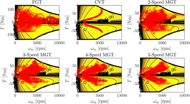
We observe the FGT yielding the worst performance. The main reason for this is that, owing to the towing constraint (7), the EM needs to be able to deliver a high torque and therefore has a larger size compared to the other transmissions. This effect, combined with the FGT inability of choosing the EM speed in turn results in a lower number of operating points lying in the EM high-efficiency region. Interestingly, the CVT is also outperformed by every MGT, as the additional benefits of choosing any gear-ratio do not compensate for its higher weight and lower transmission efficiency. For the MGTs, we observe the operating points converging to the areas of high efficiency as the number of gears is increased.
The benefits of adding gear ratios reach a point of diminishing returns between a 3-speed and a 4-speed MGT. Whilst the energy losses decrease as the number of gears is increased, the increase in required mechanical energy due to the increased transmission mass causes an overall higher energy consumption.
Finally, also when including a small gear-shifting cost, the MGTs still outperform the CVT and the FGT. As a result of the decreased benefit of gear changes, the best performing transmission changes from the 3-speed MGT to the 2-speed MGT. Further figures of the EM speed and the gear-ratio trajectories over the drive cycle can be found in Appendix D.
IV-B Validation
To benchmark the optimality of our methods, we first compute the globally optimal solution for a slightly less accurate quadratic version of the EM model which can be solved to global optimality with mixed-integer quadratic programming (MIQP)—the details on the implementation can be found in Appendix B. Second, we apply the proposed methods to the same quadratic motor model and compare our results to the global optima computed via MIQP. For the FGT and the CVT, the results obtained with quadratic programming and the results obtained with the proposed methods applied on the quadratic model are identical. Solving the MIQP for a 2-speed MGT with Gurobi [25] took 15 min to converge for a fixed EM size, whilst no convergence was achieved for MGTs with 3 gear-ratios or more. The gear ratios obtained with MIQP for a 2-speed MGT are and , whilst our Algorithm 1 converged to and . The resulting total energy consumption differs less than 0.03%: a difference which can be ascribed to numerical tolerances, indicating a good agreement between our solution and the global optimum.
Finally, in order to validate the results stemming from different EM models, the results obtained with the fractional EM model (12) and the quadratic model are simulated using the original nonlinear motor data. This final step on the one hand assesses the performance that would be achieved in practice, and on the other hand validates the accuracy of our models. Fig. 5 summarizes the results obtained with our methods and their performance in simulation, showing that our proposed fractional EM model (12) can predict the energy consumption of the EM very accurately, outperforming the quadratic model for all the transmission technologies. Additional results including the optimal EM size and vehicle mass are provided in Table II in Appendix C, where we observe that both the proposed EM model and the quadratic model always result in the same EM size.
V Conclusions
This paper explored the possibility of jointly optimizing the design and control of an electric vehicle’s transmission combining convex analysis and dynamic programming. Our algorithms resulted in a computational time in the order of 100 ms, enabling us to also optimize the electric motor size via exhaustive search—we could compare 100 different sizes in less than 10 s. Our modeling approach was validated with nonlinear simulations showing an overall high accuracy, whilst the optimal solution found by our algorithm was in line with the global optimum computed via mixed-integer quadratic programming. On the design side, our results showed that for the electric vehicles under consideration, a 2-speed transmission appears to be the most efficient solution when compared to other technologies, striking the best trade-off in terms of components’ mass and control flexibility.
This work opens the field for several extensions. First, the relatively high fidelity of the proposed convex models could be leveraged for more general powertrain control and optimization problems [26]. Second, the methods could be extended to account for thermal dynamics [17]. Finally, the computational efficiency of our approach could be leveraged both in more comprehensive design studies (e.g., including the battery dynamics) and real-time control applications.
Acknowledgment
We would like to thank Mr. Olaf Korzilius, Dr. Steven Wilkins and Dr. Pascal Etman for the fruitful discussions as well as Dr. Ilse New for proofreading this paper.
References
- [1] F. Un-Noor, S. Padmanaban, L. Mihet-Popa, M. Mollah, and E. Hossain, “A comprehensive study of key electric vehicle (ev) components, technologies, challenges, impacts, and future direction of development,” Energies, vol. 10, no. 1217, 2017.
- [2] IEA, “Global ev outlook 2020,” IEA, Paris, Tech. Rep., 2020.
- [3] F. Franke, M. Günther, M. Trantow, and J. F. Krems, “Does this range suit me? range satisfaction of battery electric vehicle users,” Applied Ergonomics, vol. 65, pp. 191–199, 2017.
- [4] O. Egbue and S. Long, “Barriers to widespread adoption of electric vehicles: An analysis of consumer attitudes and perceptions,” Energy Policy, vol. 48, pp. 717–729, 2012.
- [5] V. Saini, S. Singh, S. Nv, and H. Jain, “Genetic algorithm based gear shift optimization for electric vehicles,” SAE Int. Journal of Alternative Powertrains, vol. 5, no. 2, pp. 348–356, 2016.
- [6] J. Ritzmann, A. Christon, M. Salazar, and C. H. Onder, “Fuel-optimal power split and gear selection strategies for a hybrid electric vehicle,” in SAE Int. Conf. on Engines & Vehicles, 2019.
- [7] V. Ngo, T. Hofman, M. Steinbuch, and A. Serrarens, “Optimal control of the gearshift command for hybrid electric vehicles,” IEEE Transactions on Vehicular Technology, vol. 61, no. 8, pp. 3531–3543, Oct 2012.
- [8] T. Nüesch, P. Elbert, M. Flankl, C. H. Onder, and L. Guzzella, “Convex optimization for the energy management of hybrid electric vehicles considering engine start and gearshift costs,” Energies, vol. 7, no. 2, pp. 834–856, 2014.
- [9] N. Robuschi, M. Salazar, N. Viscera, F. Braghin, and C. H. Onder, “Minimum-fuel energy management of a hybrid electric vehicle via iterative linear programming,” IEEE Transactions on Vehicular Technology, vol. 69, no. 12, pp. 14 575–14 587, 2020.
- [10] P. Duhr, G. Christodoulou, C. Balerna, M. Salazar, A. Cerofolini, and C. H. Onder, “Time-optimal gearshift and energy management strategies for a hybrid electric race car,” Applied Energy, vol. 282, no. 115980, 2020.
- [11] N. Murgovski, L. Johannesson, J. Sjöberg, and B. Egardt, “Component sizing of a plug-in hybrid electric powertrain via convex optimization,” Mechatronics, vol. 22, no. 1, pp. 106–120, 2012.
- [12] S. Ebbesen, C. Dönitz, and L. Guzzella, “Particle swarm optimization for hybrid electric drive-train sizing,” International Journal of Vehicle Design, vol. 58, no. 2–4, pp. 181–199, 2012.
- [13] T. Hofman and M. Salazar, “Transmission ratio design for electric vehicles via analytical modeling and optimization,” in IEEE Vehicle Power and Propulsion Conference, 2020.
- [14] T. Hofman and N. H. J. Janssen, “Integrated design optimization of the transmission system and vehicle control for electric vehicles,” in IFAC World Congress, 2017.
- [15] F. J. R. Verbruggen, M. Salazar, M. Pavone, and T. Hofman, “Joint design and control of electric vehicle propulsion systems,” in European Control Conference, 2020.
- [16] O. Borsboom, C. A. Fahdzyana, T. Hofman, and M. Salazar, “A convex optimization framework for minimum lap time design and control of electric race cars,” IEEE Transactions on Vehicular Technology, 2021, under review.
- [17] A. Locatello, M. Konda, O. Borsboom, T. Hofman, and M. Salazar, “Time-optimal control of electric race cars under thermal constraints,” in European Control Conference, 2021, in press.
- [18] P. Leise, L. C. Simon, and P. F. Pelz, Optimization of Complex Systems: Theory, Models, Algorithms and Applications. Springer, 2019, ch. Finding Global-Optimal Gearbox Designs for Battery Electric Vehicles.
- [19] A. Sorniotti, S. Subramanyan, A. Turner, C. Cavallino, F. Viotto, and S. Bertolotto, “Selection of the optimal gearbox layout for an electric vehicle,” SAE Int. Journal of Engines, vol. 4, no. 1, pp. 1267–1280, 2011.
- [20] B. Gao, Q. Liang, Y. Xiang, L. Guo, and H. Chen, “Gear ratio optimization and shift control of 2-speed i-amt in electric vehicle,” Mechanical Systems and Signal Processing, vol. 50-51, pp. 615–631, 2015.
- [21] M. Morozov, K. Humphries, T. Rahman, T. Zou, and J. Angeles, “Drivetrain analysis and optimization of a two-speed class-4 electric delivery truck,” in SAE World Congress, 2019.
- [22] F. J. R. Verbruggen, E. Silvas, and T. Hofman, “Electric powertrain topology analysis and design for heavy-duty trucks,” Energies, vol. 13, no. 10, 2020.
- [23] L. Guzzella and A. Sciarretta, Vehicle propulsion systems: Introduction to Modeling and Optimization, 2nd ed. Springer Berlin Heidelberg, 2007.
- [24] Ansys Motor-CAD. ANSYS, Inc. Available at https://www.ansys.com/products/electronics/ansys-motor-cad.
- [25] Gurobi Optimization, LLC. Gurobi optimizer reference manual. Available at http://www.gurobi.com.
- [26] O. Korzilius, O. Borsboom, T. Hofman, and M. Salazar, “Optimal design of electric micromobility vehicles,” in Proc. IEEE Int. Conf. on Intelligent Transportation Systems, 2021, under review. Extended version available at https://arxiv.org/abs/2104.10155.
- [27] A. Richards and J. How, “Mixed-integer programming for control,” in American Control Conference, 2005.
Appendix A Electric Motor Sizing
Similar to [15], we scale the EM linearly with its maximum power. The motor will be scaled along a scaling parameter where
| (35) |
The coefficients are then scaled as
| (36) |
Appendix B Energy-optimal Solution of Problem 1 via Mixed-integer Quadratic Programming
The iterative Algorithm 1 we devised to jointly optimize the design and operation of an MGT does not provide global optimality guarantees. However, we can perform a numerical benchmark to check the proximity of our solution to the global optimum obtained with mixed-integer convex programming. However, given the mathematical structure of our problem, to the best of the authors’ knowledge there are no off-the-shelf mixed-integer convex programming algorithms available that could solve it to global optimality. Therefore, we use a slightly less accurate quadratic version of the EM model and solve Problem 1 both with our Algorithm 1 and mixed-integer quadratic programming (MIQP). Specifically, we model the EM as
| (37) |
where , and are determined as in Section 1, and then frame Problem 1 as a MIQP using the big- method [27]. First, we relax the losses as
| (38) |
This relaxation is lossless and will hold with equality if the total energy is minimized. The EM speed is determined by
| (39) | ||||
and we ensure that one gear is selected with
| (40) |
Finally, we formulate the objective function as the sum of the EM losses as
| (41) |
where , and frame Problem 1 as an MIQP as follows.
Problem 2 (Mixed-Integer Quadratic Problem).
Given the electric vehicle architecture of Fig. 1 equipped with an MGT, the optimal gear-ratios and gear-trajectory are the solution of
Appendix C Vehicle Parameters and Optimization Results
| Parameter | Symbol | Value | Unit |
|---|---|---|---|
| Vehicle base mass | 1450 | kg | |
| CVT mass | 80 | kg | |
| FGT and MGT base mass | 50 | kg | |
| added mass per gear | 5 | kg/gear | |
| CVT efficiency | 0.96 | - | |
| FGT efficiency | 0.98 | - | |
| MGT efficiency | 0.98 | - | |
| Wheel radius | 0.316 | m | |
| Air drag coefficient | 0.29 | - | |
| Frontal area | 0.725 | m2 | |
| Air density | 1.25 | kg/ | |
| Rolling resistance coefficient | 0.02 | - | |
| Gravitational constant | 9.81 | m/ | |
| Minimal Slope | 25 | ° | |
| Gearshift Cost | 300 | J | |
| Threshold Parameter | 0.0001 | % | |
| Transmission |
Total
Energy |
Energy Loss | Vehicle Mass | Max Power |
|---|---|---|---|---|
| FGT | 9.277 MJ | 804.5 kJ | 1563 kg | 64 kW |
| 2-Speed MGT | 8.968 MJ | 548.9 kJ | 1551 kg | 45 kW |
| 3-Speed MGT | 8.962 MJ | 520.8 kJ | 1556 kg | 45 kW |
| 4-Speed MGT | 8.973 MJ | 510.1 kJ | 1561 kg | 45 kW |
| 5-Speed MGT | 8.988 MJ | 503.6 kJ | 1566 kg | 45 kW |
| CVT | 9.189 MJ | 499.4 kJ | 1572 kg | 47 kW |
| 2-Speed MGT with Shift-Cost | 8.973 MJ | 554.5 kJ | 1551 kg | 45 kW |
| 3-Speed MGT with Shift-Cost | 8.976 MJ | 535.6 kJ | 1556 kg | 45 kW |
| 4-Speed MGT with Shift-Cost | 8.990 MJ | 526.8 kJ | 1561 kg | 45 kW |
| 5-Speed MGT with Shift-Cost | 9.009 MJ | 524.0 kJ | 1566 kg | 45 kW |
Appendix D Optimal Speed and Gear Trajectories
Fig. 6 shows the optimal EM speed and gear-ratio trajectories for the EV equipped with an FGT and a CVT. The CVT is able to vary the gear ratios and therefore the range of values for the EM speed is smaller than in the case of the FGT.
Fig. 7 and 8 show the EM speed and gear-ratio trajectories resulting from Algorithm 1 without gear-shifting costs. Going from a 2-speed to a 4-speed MGT, the increase in gears leads to a better control of the EM speed. In Fig. 8, the diminishing returns of an added gear become visible for the 4-speed and 5-speed configurations, as the difference in the EM speed becomes smaller.
Fig. 9 and 10 show the optimal EM speed and gear values for an MGT when including gear-shifting costs, whereby, compared to Fig. 7 and 8, we observe a clear reduction in the number of gear shifts.