跳到论文正文
W Papers独立论文阅读器 arXiv:2105.05102 论文正文 计算阅读时间 · 0%
引用这篇论文根据当前论文元数据生成,正式投稿前建议核对。


License: arXiv.org perpetual non-exclusive license
arXiv:2105.05102v3 [cs.RO] 10 Jan 2022

Efficient Analytical Derivatives of Rigid-Body Dynamics using Spatial Vector Algebra

Shubham Singh Affiliation: Graduate Research Assistant, Aerospace Engineering, The University of Texas at Austin, TX-78751, USA. singh281@utexas.edu    Ryan P. Russell Affiliation: Associate Professor, Aerospace Engineering, The University of Texas at Austin, TX-78751, USA. ryan.russell@utexas.edu    Patrick M. Wensing Affiliation: Assistant Professor, Aerospace & Mechanical Engineering, University of Notre Dame, IN-46556, USA. pwensing@nd.edu
Abstract

An essential need for many model-based robot control algorithms is the ability to quickly and accurately compute partial derivatives of the equations of motion. State of the art approaches to this problem often use analytical methods based on the chain rule applied to existing dynamics algorithms. Although these methods are an improvement over finite differences in terms of accuracy, they are not always the most efficient. In this paper, we contribute new closed-form expressions for the first-order partial derivatives of inverse dynamics, leading to a recursive algorithm. The algorithm is benchmarked against chain-rule approaches in Fortran and against an existing algorithm from the Pinocchio library in C++. Tests consider computing the partial derivatives of inverse and forward dynamics for robots ranging from kinematic chains to humanoids and quadrupeds. Compared to the previous open-source Pinocchio implementation, our new analytical results uncover a key computational restructuring that enables efficiency gains. Speedups of up to 1.4x are reported for calculating the partial derivatives of inverse dynamics for the 50-dof Talos humanoid.

I Introduction

[b] Method Implementation (Easy/Medium/Hard) Speed (Slow/Medium/Fast) Accuracy (Low/Medium/High) Finite Difference [8, 9, 7] Easy Medium Low Complex-step Differentiation [13, 14] Easy Slow/Medium High Automatic Differentiation [10, 11, 4] Easy/Medium Slow/Medium High Analytical Chain-Rule Differentiation [15],[5]1 Medium/Hard Medium High Special-Purpose Analytical Method [17, 18],[6]2, [This Paper]3 Hard Medium/Fast High

TABLE I: Rough summary of methods to calculate partial derivatives of rigid-body dynamics.
  • 1

    Algo-2,3 of [5] provides a chain-rule method for ID partial derivatives.

  • 2

    Pinocchio code for ID partial derivatives accompanying [5] but different from chain-rule.

  • 3

    This paper provides a Special-Purpose Analytical Method that outperforms the state-of-the-art in terms of speed.

Rigid-body dynamics models are widely used in the development of control algorithms for quadruped and humanoid robots, with recursive dynamics algorithms at the core of many real-time controllers. Example use cases include current approaches to controller design via optimization [1, 2]. Likewise, robotics libraries such as Crocoddyl [3] and Drake [4] require the partial derivatives of rigid-body dynamics with respect to the state and control variables. The calculation of these derivatives represents the majority of the CPU time required in many optimal control applications [5].

There are multiple general-purpose methods that can be applied to rigid-body dynamics for computing derivatives. Finite differences [8, 9, 7] are simple to implement and are trivially parallelized, but suffer in accuracy (Table I). The complex-step method [12] is accurate to machine precision but requires all functions to be computed in the complex plane, leading to additional overhead. Cossette et al. [13] extended this method to matrix Lie groups, providing direct applicability to rigid-body dynamics. An approach that avoids the overhead of the complex step is automatic differentiation (AD), also called algorithmic differentiation [10, 11, 4]. AD calculates the partials of an algorithm by automating the accumulation of chain-rule expressions through operator overloading [10] or source code transformation [4, 11]. The first approach overloads basic data types to compute partials concurrently with all arithmetic. The second approach builds an expression graph from source code and augments the source directly to calculate the partial derivatives.

Without relying on AD, but similar to it, others have developed analytical methods that accumulate chain-rule expressions on top of existing algorithms. Examples include many existing descriptions of recursive algorithms for dynamics derivatives [15, 5, 16]. The derivation in Ref. [5] applies chain rule on the classical two-pass Recursive-Newton-Euler Algorithm (RNEA) for inverse dynamics (ID). The presented method has computational complexity O⁡(N​d)O(Nd) for both the forward and backward pass of the RNEA derivatives, where NN is the number of bodies in the system and dd is the depth of the kinematic connectivity tree. However, the algorithm in the C++ Pinocchio (2.6.0) code [6] associated with [5] is distinctly different from the algorithm presented in [5]. The Pinocchio code includes a more efficient O⁡(N)O(N) forward pass, coupled with an O⁡(N​d)O(Nd) backward pass.

Derivative algorithms that directly carry out chain-rule on an existing algorithm (using AD or by hand) may not always be the most efficient. Other special-purpose methods have been proposed to fully exploit the structure of the rigid-body equations of motion. Such approaches often analytically differentiate closed-form equations of motion and then design an algorithm to compute the result. An example is Ref. [17] where partial derivatives are considered of the mass matrix 𝑴⁡(𝒒)\boldsymbol{M}(\boldsymbol{q}), the Coriolis matrix 𝑪⁡(𝒒,𝒒˙)\boldsymbol{C}(\boldsymbol{q},\dot{\boldsymbol{q}}), and the gravity vector 𝒈⁡(𝒒)\boldsymbol{g}(\boldsymbol{q}) with respect to the state variables 𝒒\boldsymbol{q} and 𝒒˙\dot{\boldsymbol{q}}, leading to an 𝒪⁡(N3)\mathcal{O}(N^{3}) algorithm.

Ref. [18] gives a recursive method for partial derivatives of inverse and forward dynamics (FD) for serial kinematic chains with single-DoF joints. Their approach includes an 𝒪⁡(N2)\mathcal{O}(N^{2}) algorithm for the partials of FD, and an 𝒪⁡(N​d)\mathcal{O}(Nd) algorithm for the partials of ID.

The main contribution of this paper is to extend previous analytical results on partial derivatives of ID [18] to generic multi-DoF joint robots with a fixed or floating base. We first derive closed-form expressions for the first-order partial derivatives of ID. To the best of authors’ knowledge, these results represent the first of their kind for general rigid-body systems (fixed or floating base) with multi-DoF joints. The new expressions lead immediately to an algorithm of order 𝒪⁡(N​d)\mathcal{O}(Nd) that naturally generalizes the one shown in [18]. The method is fundamentally different than the straight chain-rule approach presented in [5]. However, the distinct algorithm in the Pinocchio code [6] ends up being directly related to the computations required in our algorithm. Despite the similarity, our new closed-form expressions uncover a key restructuring that accelerates computations. We use the relationship between FD and ID [5, 18] in an efficient manner to ultimately calculate the partial derivatives of FD with complexity 𝒪⁡(N2)\mathcal{O}(N^{2}).

II Derivatives of Rigid-Body Dynamics

Rigid-Body Dynamics: For a rigid-body system, the state variables are the configuration 𝒒\boldsymbol{q} and the generalized velocity vector 𝒒˙\dot{\boldsymbol{q}}, while the control variable is the generalized torque vector 𝝉\boldsymbol{\tau}. The equation of motion, also called the Inverse Dynamics (ID), is given by

𝝉\displaystyle\boldsymbol{\tau} =𝑴⁡(𝒒)​𝒒¨+𝑪⁡(𝒒,𝒒˙)​𝒒˙+𝒈⁡(𝒒)\displaystyle=\boldsymbol{M}(\boldsymbol{q})\ddot{\boldsymbol{q}}+\boldsymbol{C}(\boldsymbol{q},\dot{\boldsymbol{q}})\dot{\boldsymbol{q}}+\boldsymbol{g}(\boldsymbol{q}) (1)
=I​D​(m​o​d​e​l,𝒒,𝒒˙,𝒒¨)\displaystyle=ID(model,\boldsymbol{q},\dot{\boldsymbol{q}},\ddot{\boldsymbol{q}}) (2)

where 𝑴∈ℝn×n\boldsymbol{M}\in\mathbb{R}^{n\times n} is the mass matrix, 𝑪∈ℝn×n\boldsymbol{C}\in\mathbb{R}^{n\times n} is a Coriolis matrix, and 𝒈∈ℝn\boldsymbol{g}\in\mathbb{R}^{n} is the vector of generalized gravitational forces, and nn is the DoF of the system. For a fixed state, ID calculates 𝝉\boldsymbol{\tau} for a given 𝒒¨\ddot{\boldsymbol{q}} (Eq. 1), and Forward Dynamics (FD) computes 𝒒¨\ddot{\boldsymbol{q}} for a given 𝝉\boldsymbol{\tau}:

𝒒¨\displaystyle\ddot{\boldsymbol{q}} =𝑴−1​(𝒒)​(𝝉−𝑪⁡(𝒒,𝒒˙)​𝒒˙−𝒈⁡(𝒒))\displaystyle=\boldsymbol{M}^{-1}(\boldsymbol{q})\left(\boldsymbol{\tau}-\boldsymbol{C}(\boldsymbol{q},\dot{\boldsymbol{q}})\dot{\boldsymbol{q}}-\boldsymbol{g}(\boldsymbol{q})\right) (3)
=F​D​(m​o​d​e​l,𝒒,𝒒˙,𝝉)\displaystyle=FD(model,\boldsymbol{q},\dot{\boldsymbol{q}},\boldsymbol{\tau}) (4)

Toward supporting control applications (e.g., [1, 9]), the objective of this work is to compute the partial derivatives of FD with respect to the state (𝒒\boldsymbol{q},𝒒˙\dot{\boldsymbol{q}}) and control variables (𝝉\boldsymbol{\tau}). The most efficient algorithms for calculating ID and FD are the 𝒪⁡(N)\mathcal{O}(N) Recursive-Newton-Euler Algorithm (RNEA) and the Articulated-Body Algorithm (ABA) respectively [19].

Derivatives of Inverse and Forward Dynamics: As presented in [5], a direct approach to compute the partial derivatives of ID is to manually differentiate the RNEA algorithm via chain-rule, denoted as RNEACR (Table II). A similar chain rule approach for the derivatives of ABA is denoted as ABACR. Because the ABA is more computationally intensive than RNEA, a more efficient approach for derivatives of FD first applies RNEACR, and then uses the relationship [5, 18]

∂F​D∂𝒖|𝒒0,𝒒˙0,𝝉0=−𝑴−1(𝒒0)∂I​D∂𝒖|𝒒0,𝒒˙0,𝒒¨0\frac{\partial~FD}{\partial\boldsymbol{u}}\biggr\rvert_{\boldsymbol{q}_{0},\dot{\boldsymbol{q}}_{0},\boldsymbol{\tau}_{0}}=-\boldsymbol{M}^{-1}(\boldsymbol{q}_{0})\frac{\partial~ID}{\partial\boldsymbol{u}}\biggr\rvert_{\boldsymbol{q}_{0},\dot{\boldsymbol{q}}_{0},\ddot{\boldsymbol{q}}_{0}} (5)

where the variable 𝒖∈{𝒒{\boldsymbol{u}}\in\{\boldsymbol{q}, 𝒒˙}\dot{\boldsymbol{q}}\}. From Eq. 3, ∂F​D/∂𝝉\partial FD/\partial\boldsymbol{\tau} can be directly calculated as 𝑴−1\boldsymbol{M}^{-1}, enabling re-use in Eq. 5. This method for the partials of FD via RNEA Chain Rule is abbreviated as FDCR.

The state-of-the-art numerical method for computing partial derivatives of FD is provided in the Pinocchio package [6] (Pinocchio FD Derivs, Table II). The method first computes the derivatives of ID (Pinocchio ID Derivs, Table II). It then computes 𝑴−1\boldsymbol{M}^{-1} and uses Eq. 5 to obtain the derivatives of FD.

In the following sections, Spatial Vector Algebra (SVA) is reviewed for dynamics analysis, followed by a theoretical development of analytical expressions that lead to an algorithm for partial derivatives of ID. The new expressions result in algorithm with a key difference from the state-of-the-art [6], enabling a speedup over it.

III Spatial Vector Algebra (SVA)

  Quantity Abbreviation Algorithm
 ∂I​D∂𝒒\frac{\partial ID}{\partial\boldsymbol{q}}, ∂I​D∂𝒒˙\frac{\partial ID}{\partial\dot{\boldsymbol{q}}} RNEACR Forward Accumulation of Chain Rule on RNEA [5, Algo. 2 &3]
Pinocchio ID Derivs Pinocchio Original Algorithm [6]
IDSVA Proposed Algorithm using SVA (Algorithm 1)
 ∂F​D∂𝒒\frac{\partial FD}{\partial\boldsymbol{q}}, ∂F​D∂𝒒˙\frac{\partial FD}{\partial\dot{\boldsymbol{q}}} ABACR Forward Chain Rule on ABA
FDCR RNEACR, Compute 𝑴−1\boldsymbol{M}^{-1} [25], Apply Eq. 5
Pinocchio FD Derivs Pinocchio ID Derivs, Compute 𝑴−1\boldsymbol{M}^{-1} [25], Apply Eq. 5
FDSVA IDSVA, Compute 𝑴−1\boldsymbol{M}^{-1} [25], use DMM/AZA depending on NN for Eq. 5
 A​B​A​(𝒒,0,𝒃,0)ABA(\boldsymbol{q},0,\boldsymbol{b},0) AZA Simplified ABA with select zero inputs for Eq. 5
 
TABLE II: Abbreviations of various algorithms/methods used. The bold acronyms are contributions from the current paper.

Notation: Spatial vectors are 6D vectors that combine the linear and angular aspects of a rigid-body motion or net force [19]. Spatial vectors are denoted with lower-case bold letters (e.g., 𝒂\boldsymbol{a}), while matrices are denoted with capitalized bold letters (e.g., 𝑨\boldsymbol{A}). Motion vectors, such as velocity and acceleration, belong to a 6D vector space denoted M6M^{6}. Spatial vectors are usually expressed in either the ground coordinate frame or a body coordinate (local coordinate) frame. For example, the spatial velocity 𝒗kk∈M6{}^{k}\boldsymbol{v}_{k}\in M^{6} of a body kk expressed in the body frame is given by 𝒗kk=[ωTkkvTkk]T{}^{k}\boldsymbol{v}_{k}=\begin{bmatrix}{}^{k}\omega_{k}^{T}&{}^{k}v_{k}^{T}\end{bmatrix}^{T} where ωkk∈ℝ3{}^{k}\omega_{k}\in\mathbb{R}^{3} is the angular velocity expressed in a coordinate frame fixed to the body, while vkk∈ℝ3{}^{k}v_{k}\in\mathbb{R}^{3} is the linear velocity of the origin of the body frame. When expressed in the ground frame, the spatial velocity for body kk is denoted as 𝒗k0{}^{0}\boldsymbol{v}_{k}. The vector is again composed of angular and linear velocity components. However, the linear velocity is associated with the body-fixed point on body kk that is coincident with the origin of the ground frame 00. In this paper, when the frame used to express a spatial vector is omitted, the ground frame is assumed.

Force-like vectors, such as force and momentum, belong to another 6D vector space F6F^{6}, which is dual to M6M^{6}. A spatial cross-product between two motion vectors (𝒗\boldsymbol{v},𝒖\boldsymbol{u}), written as (𝒗×)𝒖(\boldsymbol{v}\times)\boldsymbol{u}, is given by (Eq. 6). This operation can be understood as providing the time rate of change of 𝒖\boldsymbol{u}, when 𝒖\boldsymbol{u} is moving with a spatial velocity 𝒗\boldsymbol{v}. For a Cartesian vector, the matrix ω×\omega\times is the classical 3D cross product operator. A spatial cross-product between a motion and a force vector is written as (𝒗×∗)𝒇(\boldsymbol{v}\times^{*})\boldsymbol{f}, as defined in Eq. 7.

𝒗×=[ω×𝟎v×ω×]\displaystyle\boldsymbol{v}\times=\begin{bmatrix}\omega\times&\bf{0}\\ v\times&\omega\times\end{bmatrix} (6)
𝒗×∗=[ω×v×𝟎ω×]\displaystyle\boldsymbol{v}\times^{*}=\begin{bmatrix}\omega\times&v\times\\ \bf{0}&\omega\times\end{bmatrix} (7)

An operator ׯ∗\,\overline{\!\times\!}{}^{\,*} is defined by swapping the order of the cross product, such that (𝒇ׯ)∗𝒗=(𝒗×∗)𝒇(\boldsymbol{f}\,\overline{\!\times\!}{}^{\,*})\boldsymbol{v}=(\boldsymbol{v}\times^{*})\boldsymbol{f} [20]. Further introduction to SVA is provided in Appendix -A.

Connectivity: An open-chain kinematic tree with serial or branched connectivity (Fig. 1) is considered with NN links connected by joints, each with up to 6 DoF. Body ii’s parent toward the root of the kinematic tree is denoted as λ⁡(i)\lambda(i). ν⁡(i)\nu(i) denotes the set of bodies in the subtree rooted at body ii, while ν¯​(i)\overline{\nu}(i) denotes the set of bodies in ν⁡(i)\nu(i) excluding the body ii . We define i⪯ji\preceq j if body ii is in the path from body jj to the base.

The spatial velocities of the neighbouring bodies in the tree are related by 𝒗i=𝒗λ⁡(i)+𝑺i​𝒒˙i\boldsymbol{v}_{i}=\boldsymbol{v}_{\lambda(i)}+\boldsymbol{S}_{i}\dot{\boldsymbol{q}}_{i}, where 𝑺i\boldsymbol{S}_{i} is the joint motion subspace matrix for joint ii [19] and 𝒒˙i\dot{\boldsymbol{q}}_{i} the joint rates for joint ii. For a single DoF revolute joint, 𝑺i∈ℝ6\boldsymbol{S}_{i}\in\mathbb{R}^{6}, and 𝒒˙i\dot{\boldsymbol{q}}_{i} is a scalar. For a 6-DoF free-motion joint, 𝑺i∈ℝ6×6\boldsymbol{S}_{i}\in\mathbb{R}^{6\times 6}, while 𝒒˙i∈ℝ6\dot{\boldsymbol{q}}_{i}\in\mathbb{R}^{6}. The velocity 𝒗i\boldsymbol{v}_{i} can also be written as the sum of joint velocities over predecessors as 𝒗i=∑l⪯i𝑺l​𝒒˙l\boldsymbol{v}_{i}=\sum_{l\preceq i}{\color[rgb]{0,0,0}\boldsymbol{S}_{l}}\dot{\boldsymbol{q}}_{l}. The derivative of joint motion subspace matrix due to the axis changing with respect to local coordinates (commonly denoted 𝑺̊i\mathring{\boldsymbol{S}}_{i} [19]) is assumed to be zero. The quantity 𝑺˙i=𝒗i×𝑺i{\color[rgb]{0,0,0}\,\dot{\!\boldsymbol{S}}{}_{i}}=\boldsymbol{v}_{i}\times{\color[rgb]{0,0,0}\boldsymbol{S}_{i}} signifies the rate of change of 𝑺i\boldsymbol{S}_{i} due to the local coordinate system moving.
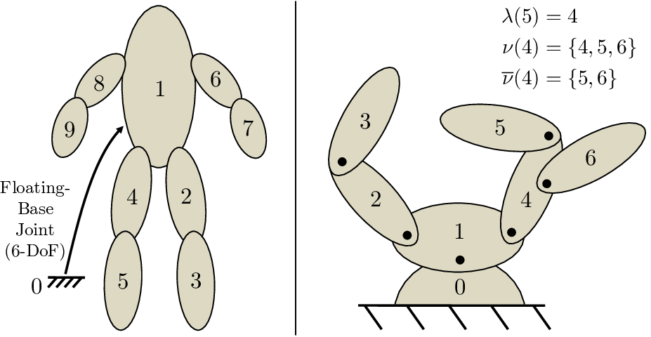
Refer to caption
Fig. 1: Body numbering and notation examples with floating- and fixed-base systems.

Dynamics: The spatial equation of motion [19] is given for body kk as:

𝒇k=𝑰​𝒂kk+𝒗k×∗𝑰​𝒗kk\boldsymbol{f}_{k}=\boldsymbol{I}{}_{k}\boldsymbol{a}_{k}+\boldsymbol{v}_{k}\times^{*}\boldsymbol{I}{}_{k}\boldsymbol{v}_{k} (8)

where 𝒇k\boldsymbol{f}_{k} is the net spatial force on body kk, 𝑰k\boldsymbol{I}{}_{k} is its spatial inertia [19], and 𝒂k\boldsymbol{a}_{k} is its spatial acceleration. Instead of treating gravity as an external force, a common trick is to accelerate the base upwards opposite of the gravitational acceleration (𝒂0=−𝒂g\boldsymbol{a}_{0}=-\boldsymbol{a}_{g}), providing the acceleration of body kk as:

𝒂k=∑l⪯k(𝑺l​𝒒¨l+𝒗l×𝑺l​𝒒˙l)+𝒂0.\boldsymbol{a}_{k}=\textstyle\sum_{l\preceq k}{\color[rgb]{0,0,0}\big(}{\color[rgb]{0,0,0}\boldsymbol{S}_{l}}\ddot{\boldsymbol{q}}_{l}+\boldsymbol{v}_{l}\times{\color[rgb]{0,0,0}\boldsymbol{S}_{l}}\dot{\boldsymbol{q}}_{l}{\color[rgb]{0,0,0}\big)}+\boldsymbol{a}_{0}\,. (9)

For later use, we decompose 𝒂k\boldsymbol{a}_{k} into terms from joint accelerations, and terms from joint rates, according to

𝜸k=∑l⪯k𝑺l​𝒒¨l​ and ​𝝃k=∑l⪯k𝒗l×𝑺l​𝒒˙l\boldsymbol{\gamma}_{k}=\textstyle\sum_{l\preceq k}{\color[rgb]{0,0,0}\boldsymbol{S}_{l}}\ddot{\boldsymbol{q}}_{l}\textrm{~~~and~~~}\boldsymbol{\xi}_{k}=\textstyle\sum_{l\preceq k}\boldsymbol{v}_{l}\times{\color[rgb]{0,0,0}\boldsymbol{S}_{l}}\dot{\boldsymbol{q}}_{l}

(𝜸,𝝃∈M6\boldsymbol{\gamma},\boldsymbol{\xi}\in M^{6}). With these definitions, 𝒂k=𝜸k+𝝃k+𝒂0\boldsymbol{a}_{k}=\boldsymbol{\gamma}_{k}+\boldsymbol{\xi}_{k}+\boldsymbol{a}_{0}.

In a similar fashion, the net spatial force on body kk is then decomposed as:

𝒇k=𝜼k+𝜻k+𝑰​𝒂0k\boldsymbol{f}_{k}=\boldsymbol{\eta}_{k}+\boldsymbol{\zeta}_{k}+\boldsymbol{I}{}_{k}\boldsymbol{a}_{0} (10)

where 𝜼k=𝑰​𝜸kk\boldsymbol{\eta}_{k}=\boldsymbol{I}{}_{k}\boldsymbol{\gamma}_{k} (𝜼∈F6\boldsymbol{\eta}\in F^{6}) is the spatial force on the body caused by joint accelerations 𝒒¨\ddot{\boldsymbol{q}}, and 𝜻k=𝒗k×∗𝑰​𝒗kk+𝑰​𝝃kk\boldsymbol{\zeta}_{k}=\boldsymbol{v}_{k}\times^{*}\boldsymbol{I}{}_{k}\boldsymbol{v}_{k}+\boldsymbol{I}{}_{k}\boldsymbol{\xi}_{k} (𝜻∈F6\boldsymbol{\zeta}{\color[rgb]{0,0,0}\in F^{6}}) gives the Coriolis and centripetal forces on body kk. From the formulation of the RNEA [19], 𝝉i=𝑺iT​𝒇iC{\color[rgb]{0,0,0}\boldsymbol{\tau}_{i}}=\boldsymbol{S}_{i}^{T}\boldsymbol{f}_{i}^{C}, where 𝒇iC=∑k⪰i𝒇k\boldsymbol{f}_{i}^{C}=\sum_{k\succeq i}\boldsymbol{f}_{k} is the spatial force transmitted across joint ii.


∂[𝑪​𝒒˙]i∂𝒒j=\displaystyle\frac{\partial[\boldsymbol{C}\dot{\boldsymbol{q}}]_{i}}{\partial{\color[rgb]{0,0,0}\boldsymbol{q}_{j}}}= 𝑺iT​[2​𝑩​𝚿˙jiC+𝑰​𝒗λ⁡(j)iC×𝚿˙j+𝑰​𝝃λ⁡(j)iC×𝑺j]\displaystyle{\color[rgb]{0,0,0}\boldsymbol{S}_{i}^{T}\Big[2\boldsymbol{B}{}_{i}^{C}\,\dot{\!\boldsymbol{\Psi}}_{j}+\boldsymbol{I}{}_{i}^{C}\boldsymbol{v}_{\lambda(j)}\times\,\dot{\!\boldsymbol{\Psi}}_{j}+}{\color[rgb]{0,0,0}\boldsymbol{I}{}_{i}^{C}\boldsymbol{\xi}_{\lambda(j)}\times\boldsymbol{S}_{j}\Big]} (26)
∂[𝑪​𝒒˙]j∂𝒒i=\displaystyle\frac{\partial[\boldsymbol{C}\dot{\boldsymbol{q}}]_{j}}{\partial{\color[rgb]{0,0,0}\boldsymbol{q}_{i}}}= 𝑺jT[2𝑩𝚿˙iCi+𝑰𝒗λ⁡(i)Ci×𝚿˙i+𝑰𝝃λ⁡(i)Ci×𝑺i+𝜻iCׯ𝑺i∗],(j≠i)\displaystyle{\color[rgb]{0,0,0}\boldsymbol{S}_{j}^{T}\Big[2\boldsymbol{B}{}_{i}^{C}\,\dot{\!\boldsymbol{\Psi}}_{i}+\boldsymbol{I}{}_{i}^{C}\boldsymbol{v}_{\lambda(i)}\times\,\dot{\!\boldsymbol{\Psi}}_{i}+}{\color[rgb]{0,0,0}\boldsymbol{I}{}_{i}^{C}\boldsymbol{\xi}_{\lambda(i)}\times\boldsymbol{S}_{i}+\boldsymbol{\zeta}_{i}^{C}\,\overline{\!\times\!}{}^{\,*}\boldsymbol{S}_{i}\Big],(j\neq i)} (27)

Proceeding to consider the system overall, for any particular joint ii, Eq. 1 can be written as follows.

𝝉i=[𝑴⁡(𝒒)​𝒒¨]i+[𝑪⁡(𝒒,𝒒˙)​𝒒˙]i+𝒈i​(𝒒){\color[rgb]{0,0,0}\boldsymbol{\tau}_{i}}=[\boldsymbol{M}(\boldsymbol{q})\ddot{\boldsymbol{q}}]_{i}+[\boldsymbol{C}(\boldsymbol{q},\dot{\boldsymbol{q}})\dot{\boldsymbol{q}}]_{i}+{\color[rgb]{0,0,0}\boldsymbol{g}_{i}}(\boldsymbol{q}) (11)

Then, using 𝝉i=𝑺iT​𝒇iC{\color[rgb]{0,0,0}\boldsymbol{\tau}_{i}}=\boldsymbol{S}_{i}^{T}\boldsymbol{f}_{i}^{C}, Eq. 9 and 11:

[𝑴⁡(𝒒)​𝒒¨]i\displaystyle[\,\boldsymbol{M}(\boldsymbol{q})\ddot{\boldsymbol{q}}\,]_{i} =𝑺iT​∑k⪰i[𝑰​𝜸kk]\displaystyle={\color[rgb]{0,0,0}\boldsymbol{S}_{i}^{T}}\sum_{k\succeq i}[\boldsymbol{I}{}_{k}\boldsymbol{\gamma}_{k}] (12)
[𝑪⁡(𝒒,𝒒˙)​𝒒˙]i\displaystyle[\,\boldsymbol{C}(\boldsymbol{q},\dot{\boldsymbol{q}})\dot{\boldsymbol{q}}\,]_{i} =𝑺iT​∑k⪰i[𝒗k×∗𝑰​𝒗kk+𝑰​𝝃kk]\displaystyle={\color[rgb]{0,0,0}\boldsymbol{S}_{i}^{T}}\sum_{k\succeq i}[\boldsymbol{v}_{k}\times^{*}\boldsymbol{I}{}_{k}\boldsymbol{v}_{k}+\boldsymbol{I}{}_{k}\boldsymbol{\xi}_{k}] (13)
𝒈i\displaystyle{\color[rgb]{0,0,0}\boldsymbol{g}_{i}} =𝑺iT​𝑰​𝒂0iC\displaystyle={\color[rgb]{0,0,0}\boldsymbol{S}_{i}^{T}\boldsymbol{I}{}_{i}^{C}\boldsymbol{a}_{0}} (14)

where 𝑰iC\boldsymbol{I}{}{}_{i}^{C} denotes the composite rigid-body inertia of the sub-tree rooted at body ii, given by 𝑰iC=∑k⪰i𝑰k\boldsymbol{I}{}{}_{i}^{C}=\sum_{k\succeq i}\boldsymbol{I}{}_{k}.

IV Analytical Partial Derivatives using SVA

In this section, closed-form expressions are derived for the derivatives of ID. The reader less interested in the derivation may skip to Eq. 30 and Eq. 32 as a summary.

IV-A Building Blocks

Several kinematic identities are given in Appendix -C as a basis for the main derivation. We denote by njn_{j} the number of DoFs for joint jj. The motion subspace matrix for the joint is then given as 𝑺j=[𝒔j,1⋯𝒔j,nj]\boldsymbol{S}_{j}=\begin{bmatrix}\boldsymbol{s}_{j,1}&\cdots\boldsymbol{s}_{j,n_{j}}\end{bmatrix} where each spatial vector 𝒔j,p\boldsymbol{s}_{j,p} gives the pp-th free-mode of motion for joint jj. With a slight liberty of notation, ∂/∂qj,p\partial/\partial q_{j,p} denotes an operator for the directional derivative along this pp-th free mode of a joint. For example, considering the case with j⪯ij\preceq i gives identity J1:

∂∂qj,p​𝑺i=𝒔j,p×𝑺i\frac{\partial}{\partial q_{j,p}}\boldsymbol{S}_{i}=\boldsymbol{s}_{j,p}\times\boldsymbol{S}_{i} (J1)

which provides the rate of change in 𝑺i\boldsymbol{S}_{i} with respect to relative motion 𝒔j,p\boldsymbol{s}_{j,p} at joint jj earlier in the chain. For revolute joints, these derivatives are just conventional derivatives with respect to joint angles. For multi-DoF joints such as a floating base, they are more formally Lie derivatives. Considering a configuration-dependent vector 𝒖\boldsymbol{u}, we denote by

∂𝒖∂𝒒j=[∂𝒖/∂qj,1⋯∂𝒖/∂qj,nj]\frac{\partial\boldsymbol{u}}{\partial\boldsymbol{q}_{j}}=\Large\begin{bmatrix}\nicefrac{{\partial\boldsymbol{u}}}{{\partial q_{j,1}}}&\cdots&\nicefrac{{\partial\boldsymbol{u}}}{{\partial q_{j,n_{j}}}}\end{bmatrix}

the matrix of derivatives associated with joint jj. To illustrate, we derive identity J7 for later use in the section.

Considering j⪯ij\preceq i and using the definition of 𝜸i\boldsymbol{\gamma}_{i}:

∂𝜸i∂qj,p=∑l⪯i∂𝑺l∂qj,p​𝒒¨l\frac{\partial\boldsymbol{\gamma}_{i}}{\partial q_{j,p}}=\sum_{l\preceq i}\frac{\partial\boldsymbol{S}_{l}}{\partial q_{j,p}}\ddot{\boldsymbol{q}}_{l} (15)

Using J1 and switching the order of the cross product:

∂𝜸i∂qj,p=−∑j⪯l⪯i𝑺l𝒒¨l×𝒔j,p\frac{\partial\boldsymbol{\gamma}_{i}}{\partial q_{j,p}}=-\sum_{j\preceq l\preceq i}\boldsymbol{S}_{l}\ddot{\boldsymbol{q}}_{l}\times\boldsymbol{s}_{j,p} (16)

Collecting all DoFs of joint jj, Eq. 80 becomes:

∂𝜸i∂𝒒j=−∑j⪯l⪯i𝑺l𝒒¨l×𝑺j\frac{\partial\boldsymbol{\gamma}_{i}}{\partial\boldsymbol{q}_{j}}=-\sum_{j\preceq l\preceq i}\boldsymbol{S}_{l}\ddot{\boldsymbol{q}}_{l}\times\boldsymbol{S}_{j} (17)

Using the definition of 𝜸l\boldsymbol{\gamma}_{l}, and summing over ll:

∂𝜸i∂𝒒j=(𝜸λ⁡(j)−𝜸i)×𝑺j\frac{\partial\boldsymbol{\gamma}_{i}}{\partial\boldsymbol{q}_{j}}=(\boldsymbol{\gamma}_{\lambda(j)}-\boldsymbol{\gamma}_{i})\times\boldsymbol{S}_{j} (18)

IV-B First-order Partial Derivatives of ID w.r.t. 𝐪\boldsymbol{q}

The subsequent derivations employ these formulae and the identities from Appendix -C to obtain the partials of the terms in Eq. 11. Since the derivations are quite lengthy, the presentation focuses on explaining the methodology. A full derivation is provided in Appendix -D.

Partial Derivative of Eq. 12: We derive the partial derivative of [𝑴⁡(𝒒)​𝒒¨]i[\boldsymbol{M}(\boldsymbol{q})\ddot{\boldsymbol{q}}]_{i} with respect to 𝒒j\boldsymbol{q}_{j} for all i,j∈{1,…,N}i,j\in\{1,\ldots,N\}. First, consider the case when j⪯ij\preceq i. Using the product rule of differentiation in Eq. 12:

∂[𝑴⁡(𝒒)​𝒒¨]i∂𝒒j=\displaystyle\frac{\partial[\boldsymbol{M}(\boldsymbol{q})\ddot{\boldsymbol{q}}]_{i}}{\partial\boldsymbol{q}_{j}}= ∂(𝑺iT)∂𝒒j​∑k⪰i[𝑰​𝜸kk]+\displaystyle\frac{\partial(\boldsymbol{S}_{i}^{T})}{\partial\boldsymbol{q}_{j}}\sum_{k\succeq i}[\boldsymbol{I}{}_{k}\boldsymbol{\gamma}_{k}]+ (19)
𝑺iT​∑k⪰i[∂𝑰k∂𝒒j​𝜸k+𝑰​∂𝜸k∂𝒒jk]\displaystyle\boldsymbol{S}_{i}^{T}\sum_{k\succeq i}\Bigg[\frac{\partial\boldsymbol{I}{}_{k}}{\partial\boldsymbol{q}_{j}}\boldsymbol{\gamma}_{k}+\boldsymbol{I}{}_{k}\frac{\partial\boldsymbol{\gamma}_{k}}{\partial\boldsymbol{q}_{j}}\Bigg]

Using identity J3 for the term ∂(𝑺iT)∂𝒒j\frac{\partial(\boldsymbol{S}_{i}^{T})}{\partial\boldsymbol{q}_{j}}, J4 for the term ∂𝑰k∂𝒒j​𝜸k\frac{\partial\boldsymbol{I}{}_{k}}{\partial\boldsymbol{q}_{j}}\boldsymbol{\gamma}_{k}, J7 for ∂𝜸k∂𝒒j\frac{\partial\boldsymbol{\gamma}_{k}}{\partial\boldsymbol{q}_{j}}, and cancelling terms:

∂[𝑴⁡(𝒒)​𝒒¨]i∂𝒒j=\displaystyle\frac{\partial[\boldsymbol{M}(\boldsymbol{q})\ddot{\boldsymbol{q}}]_{i}}{\partial\boldsymbol{q}_{j}}= 𝑺iT∑k⪰i[𝑰k(𝜸λ⁡(j)×)]𝑺j\displaystyle\boldsymbol{S}_{i}^{T}\sum_{k\succeq i}\Big[\boldsymbol{I}{}_{k}(\boldsymbol{\gamma}_{\lambda(j)}\times)\Big]\boldsymbol{S}_{j} (20)

Upon summing over the index kk, the final expression is:

∂[𝑴⁡(𝒒)​𝒒¨]i∂𝒒j=𝑺iT​[𝑰​𝜸λ⁡(j)iC×𝑺j]\frac{\partial[\boldsymbol{M}(\boldsymbol{q})\ddot{\boldsymbol{q}}]_{i}}{\partial{\color[rgb]{0,0,0}\boldsymbol{q}_{j}}}={\color[rgb]{0,0,0}\boldsymbol{S}_{i}^{T}\Big[\boldsymbol{I}{}_{i}^{C}\boldsymbol{\gamma}_{\lambda(j)}\times\boldsymbol{S}_{j}\Big]} (21)

For the case i≺ji{\color[rgb]{0,0,0}\prec}j, we have that:

∂[𝑴⁡(𝒒)​𝒒¨]i∂𝒒j=𝑺iT​∑k⪰i[∂𝑰k∂𝒒j​𝜸k+𝑰​∂𝜸k∂𝒒jk]\frac{\partial[\boldsymbol{M}(\boldsymbol{q})\ddot{\boldsymbol{q}}]_{i}}{\partial\boldsymbol{q}_{j}}=\boldsymbol{S}_{i}^{T}\sum_{k\succeq i}\Bigg[\frac{\partial\boldsymbol{I}{}_{k}}{\partial\boldsymbol{q}_{j}}\boldsymbol{\gamma}_{k}+\boldsymbol{I}{}_{k}\frac{\partial\boldsymbol{\gamma}_{k}}{\partial\boldsymbol{q}_{j}}\Bigg] (22)

Using the identities J3, J4 and J7 and cancelling terms:

∂[𝑴⁡(𝒒)​𝒒¨]i∂𝒒j=𝑺iT∑k⪰j[(𝑰k𝜸k)ׯ∗+𝑰k(𝜸λ⁡(j)×)]𝑺j\displaystyle\frac{\partial[\boldsymbol{M}(\boldsymbol{q})\ddot{\boldsymbol{q}}]_{i}}{\partial\boldsymbol{q}_{j}}=\boldsymbol{S}_{i}^{T}\sum_{k\succeq j}\Big[(\boldsymbol{I}{}_{k}\boldsymbol{\gamma}_{k})\,\overline{\!\times\!}{}^{\,*}+\boldsymbol{I}{}_{k}(\boldsymbol{\gamma}_{\lambda(j)}\times)\Big]\boldsymbol{S}_{j} (23)

Summing over the index kk results in:

∂[𝑴⁡(𝒒)​𝒒¨]i∂𝒒j=𝑺iT[𝜼jCׯ+∗𝑰(𝜸λ⁡(j)×)Cj]𝑺j\frac{\partial[\boldsymbol{M}(\boldsymbol{q})\ddot{\boldsymbol{q}}]_{i}}{\partial{\color[rgb]{0,0,0}\boldsymbol{q}_{j}}}={\color[rgb]{0,0,0}\boldsymbol{S}_{i}^{T}\Big[\boldsymbol{\eta}_{j}^{C}\,\overline{\!\times\!}{}^{\,*}+\boldsymbol{I}{}_{j}^{C}(\boldsymbol{\gamma}_{\lambda(j)}\times)\Big]\boldsymbol{S}_{j}} (24)

where 𝜼jC\boldsymbol{\eta}_{j}^{C} collects joint-acceleration-dependent forces for the subtree, calculated as 𝜼jC=∑k⪰j𝜼k\boldsymbol{\eta}_{j}^{C}=\sum_{k\succeq j}\boldsymbol{\eta}_{k} .

For ease of implementation, we consider a single case where j⪯ij\preceq i. The indices ii and jj are switched in Eq. 24, to get the expression for ∂[𝑴⁡(𝒒)​𝒒¨]j∂𝒒i\frac{\partial[\boldsymbol{M}(\boldsymbol{q})\ddot{\boldsymbol{q}}]_{j}}{\partial\boldsymbol{q}_{i}} for the case j≺ij\prec i. Therefore, Eq. 25 gives the two expressions formulated for the general case j⪯ij\preceq i.

∂[𝑴⁡(𝒒)​𝒒¨]i∂𝒒j=𝑺iT​[𝑰​𝜸λ⁡(j)iC×𝑺j]\displaystyle\frac{\partial[\boldsymbol{M}(\boldsymbol{q})\ddot{\boldsymbol{q}}]_{i}}{\partial{\color[rgb]{0,0,0}\boldsymbol{q}_{j}}}={\color[rgb]{0,0,0}\boldsymbol{S}_{i}^{T}\Big[\boldsymbol{I}{}_{i}^{C}\boldsymbol{\gamma}_{\lambda(j)}\times\boldsymbol{S}_{j}\Big]} (25)
∂[𝑴⁡(𝒒)​𝒒¨]j∂𝒒i=𝑺jT[𝜼iCׯ+∗𝑰𝜸λ⁡(i)Ci×]𝑺i,(j≠i)\displaystyle\frac{\partial[\boldsymbol{M}(\boldsymbol{q})\ddot{\boldsymbol{q}}]_{j}}{\partial{\color[rgb]{0,0,0}\boldsymbol{q}_{i}}}={\color[rgb]{0,0,0}\boldsymbol{S}_{j}^{T}\Big[\boldsymbol{\eta}_{i}^{C}\,\overline{\!\times\!}{}^{\,*}+\boldsymbol{I}{}_{i}^{C}\boldsymbol{\gamma}_{\lambda(i)}\times\Big]\boldsymbol{S}_{i},(j\neq i)}

Partial Derivative of Eq. 13: Similarly, we use identities J2-J6 (Appendix -C) to get the first-order partial derivatives of [𝑪⁡(𝒒,𝒒˙)​𝒒˙]i[\boldsymbol{C}(\boldsymbol{q},\dot{\boldsymbol{q}})\dot{\boldsymbol{q}}]_{i} with respect to 𝒒j\boldsymbol{q}_{j} for the case j⪯ij\preceq i as shown in Eq. 26, 27.

In these equations, the composite of 𝜻iC\boldsymbol{\zeta}_{i}^{C} for the subtree is defined as 𝜻iC=∑k⪰i𝜻k\boldsymbol{\zeta}{}_{i}^{C}=\sum_{k\succeq i}\boldsymbol{\zeta}_{k}, and the matrix 𝑩(𝒗k,𝑰)kk\boldsymbol{B}{}_{k}(\boldsymbol{v}_{k},\boldsymbol{I}{}_{k}) is a body-level Coriolis matrix [21, 22, 20] given by:

𝑩=k12[(𝒗k×∗)𝑰−k𝑰(𝒗k×)k+(𝑰𝒗kk)ׯ]∗\boldsymbol{B}{}_{k}=\frac{1}{2}\big[\big(\boldsymbol{v}_{k}\times^{*}\big)\boldsymbol{I}{}_{k}-\boldsymbol{I}{}_{k}\big(\boldsymbol{v}_{k}\times\big)+\big(\boldsymbol{I}{}_{k}\boldsymbol{v}_{k}\big)\,\overline{\!\times\!}{}^{\,*}\big] (28)

with its composite 𝑩iC=∑k⪰i𝑩k\boldsymbol{B}{}{}_{i}^{C}=\sum_{k\succeq i}\boldsymbol{B}{}_{k}.

Partial Derivative of the Gravity Term: Using the identities J3 and J4, for the case j⪯ij\preceq i, the partial derivative of 𝒈i\boldsymbol{g}_{i} (Eq. 14) with respect to 𝒒j\boldsymbol{q}_{j} is:

∂𝒈i∂𝒒j=𝑺iT𝑰iC(𝒂0×𝑺j)\displaystyle\frac{\partial{\color[rgb]{0,0,0}\boldsymbol{g}_{i}}}{\partial{\color[rgb]{0,0,0}\boldsymbol{q}_{j}}}={\color[rgb]{0,0,0}\boldsymbol{S}_{i}^{T}\boldsymbol{I}{}_{i}^{C}(\boldsymbol{a}_{0}\times\boldsymbol{S}_{j})} (29)
∂𝒈j∂𝒒i=𝑺jT[(𝑰iC𝒂0)ׯ∗+𝑰iC(𝒂0×)]𝑺i,(j≠i)\displaystyle\frac{\partial{\color[rgb]{0,0,0}\boldsymbol{g}_{j}}}{\partial{\color[rgb]{0,0,0}\boldsymbol{q}_{i}}}={\color[rgb]{0,0,0}\boldsymbol{S}_{j}^{T}\Big[(\boldsymbol{I}{}_{i}^{C}\boldsymbol{a}_{0})\,\overline{\!\times\!}{}^{\,*}+\boldsymbol{I}{}_{i}^{C}(\boldsymbol{a}_{0}\times)\Big]\boldsymbol{S}_{i},(j\neq i)}

Summary for Partials of ID w.r.t. q\boldsymbol{q}: The partials of the individual components are now collected together.

Terms in Eqs. 25, 26, 27, and 29 are added to get the total expressions for ∂𝝉∂𝒒\frac{\partial\boldsymbol{\tau}}{\partial\boldsymbol{q}} for the case j⪯ij\preceq i. The full derivation is provided in Appendix -E.

∂𝝉i∂𝒒j=\displaystyle\frac{\partial{\color[rgb]{0,0,0}\boldsymbol{\tau}_{i}}}{\partial{\color[rgb]{0,0,0}\boldsymbol{q}_{j}}}= 𝑺iT[2𝑩]Ci𝚿˙+j𝑺iT𝑰𝚿¨Cij\displaystyle{\color[rgb]{0,0,0}\boldsymbol{S}_{i}^{T}\big[2\boldsymbol{B}{}_{i}^{C}\big]\,\dot{\!\boldsymbol{\Psi}}{}_{j}+\boldsymbol{S}_{i}^{T}\boldsymbol{I}{}_{i}^{C}\,\ddot{\!\boldsymbol{\Psi}}{}_{j}} (30)
∂𝝉j∂𝒒i=\displaystyle\frac{\partial{\color[rgb]{0,0,0}\boldsymbol{\tau}_{j}}}{\partial{\color[rgb]{0,0,0}\boldsymbol{q}_{i}}}= 𝑺jT[2𝑩𝚿˙iCi+𝑰𝚿¨iCi+(𝒇iC)ׯ𝑺i∗](j≠i)\displaystyle{\color[rgb]{0,0,0}\boldsymbol{S}_{j}^{T}[2\boldsymbol{B}{}_{i}^{C}\,\dot{\!\boldsymbol{\Psi}}_{i}+\boldsymbol{I}{}_{i}^{C}\,\ddot{\!\boldsymbol{\Psi}}_{i}+(\boldsymbol{f}_{i}^{C})\,\overline{\!\times\!}{}^{\,*}\boldsymbol{S}_{i}](j\neq i)}

The spatial quantities 𝚿˙j\,\dot{\!\boldsymbol{\Psi}}_{j} and 𝚿¨j\,\ddot{\!\boldsymbol{\Psi}}_{j} are defined as:

𝚿˙j=𝒗λ⁡(j)×𝑺j𝚿¨j=𝒂λ⁡(j)×𝑺j+𝒗λ⁡(j)×𝚿˙j\displaystyle\begin{split}{\color[rgb]{0,0,0}\,\dot{\!\boldsymbol{\Psi}}_{j}=}&{\color[rgb]{0,0,0}\boldsymbol{v}_{\lambda(j)}\times\boldsymbol{S}_{j}}\\ {\color[rgb]{0,0,0}\,\ddot{\!\boldsymbol{\Psi}}_{j}=}&{\color[rgb]{0,0,0}\boldsymbol{a}_{\lambda(j)}\times\boldsymbol{S}_{j}+\boldsymbol{v}_{\lambda(j)}\times\,\dot{\!\boldsymbol{\Psi}}_{j}}\end{split} (31)

IV-C First-Order Partial Derivatives of ID w.r.t. 𝐪˙\dot{\boldsymbol{q}}

The partials of 𝝉\boldsymbol{\tau} with respect to 𝒒˙\dot{\boldsymbol{q}} depend only on the the Coriolis terms 𝑪​𝒒˙\boldsymbol{C}\dot{\boldsymbol{q}}. Using the identities J8 and J9 leads to expressions for the case when j⪯ij\preceq i(see Appendix -F for full derivation):

∂𝝉i∂𝒒˙j=∂[𝑪​𝒒˙]i∂𝒒˙j=𝑺iT[2𝑩iC𝑺j+𝑰iC(𝚿˙j+𝑺˙j)]\displaystyle\frac{\partial{\color[rgb]{0,0,0}\boldsymbol{\tau}_{i}}}{\partial{\color[rgb]{0,0,0}\dot{\boldsymbol{q}}_{j}}}=\frac{\partial[\boldsymbol{C}\dot{\boldsymbol{q}}]_{i}}{\partial{\color[rgb]{0,0,0}\dot{\boldsymbol{q}}_{j}}}={\color[rgb]{0,0,0}\boldsymbol{S}_{i}^{T}\Big[2\boldsymbol{B}{}_{i}^{C}\boldsymbol{S}_{j}+\boldsymbol{I}{}_{i}^{C}(\,\dot{\!\boldsymbol{\Psi}}_{j}+\,\dot{\!\boldsymbol{S}}_{j})\Big]} (32)
∂𝝉j∂𝒒˙i=∂[𝑪​𝒒˙]j∂𝒒˙i=𝑺jT[2𝑩iC𝑺i+𝑰iC(𝚿˙i+𝑺˙i)](j≠i)\displaystyle\frac{\partial{\color[rgb]{0,0,0}\boldsymbol{\tau}_{j}}}{\partial{\color[rgb]{0,0,0}\dot{\boldsymbol{q}}_{i}}}=\frac{\partial[\boldsymbol{C}\dot{\boldsymbol{q}}]_{j}}{\partial{\color[rgb]{0,0,0}\dot{\boldsymbol{q}}_{i}}}={\color[rgb]{0,0,0}\boldsymbol{S}_{j}^{T}\Big[2\boldsymbol{B}{}_{i}^{C}\boldsymbol{S}_{i}+\boldsymbol{I}{}_{i}^{C}(\,\dot{\!\boldsymbol{\Psi}}_{i}+\,\dot{\!\boldsymbol{S}}_{i})\Big](j\neq i)}

IV-D Algorithm for First-Order Partials of ID

Algorithm 1 returns the terms in Eq. 30 and Eq. 32 and has computational complexity 𝒪⁡(N​d)\mathcal{O}(Nd). The method operates with all spatial vectors expressed in ground frame coordinates. The first pass is in the forward direction and goes from root to leaves calculating the spatial velocity, acceleration, 𝑺˙i\,\dot{\!\boldsymbol{S}}_{i}, 𝚿˙i\,\dot{\!\boldsymbol{\Psi}}_{i}, 𝚿¨i\,\ddot{\!\boldsymbol{\Psi}}_{i}, 𝑩i\boldsymbol{B}{}_{i} and the spatial force 𝒇i\boldsymbol{f}_{i}. When joint ii has a single DoF, 𝑺˙i=𝚿˙i\,\dot{\!\boldsymbol{S}}_{i}=\,\dot{\!\boldsymbol{\Psi}}_{i} and 𝑺¨i=𝚿¨i\ddot{\boldsymbol{S}}_{i}=\,\ddot{\!\boldsymbol{\Psi}}_{i} and the steps are the same as in [18, Alg. 2].

The second pass progresses in the backward direction from leaves to the root. Index ii takes all the values from 1 to NN. The quantity ∂𝝉∂𝒒​[ν​(i),i]\frac{\partial\boldsymbol{\tau}}{\partial\boldsymbol{q}}[\nu(i),i] denotes the partial derivatives of 𝝉\boldsymbol{\tau} for all bodies in the sub-tree of ii with respect to 𝒒i\boldsymbol{q}_{i}, while ∂𝝉∂𝒒​[i,ν¯​(i)]\frac{\partial\boldsymbol{\tau}}{\partial\boldsymbol{q}}[i,\overline{\nu}(i)] is the partial derivative of 𝝉\boldsymbol{\tau} for body ii with respect to each of the bodies in the sub-tree of ii, excluding body ii. This backward pass again generalizes the one in [18, Alg. 2]. The differences are that the third term on line 15 can be dropped in the single-DoF case (since 𝑺iT(𝒇iCׯ)∗𝑺i=0{\boldsymbol{S}}_{i}^{T}(\boldsymbol{f}_{i}^{C}\,\overline{\!\times\!}{}^{\,*}){\boldsymbol{S}}_{i}=0 in that case), while lines 17-20 restructure a second inner loop in [18] into matrix multiplies.

Algorithm 1 IDSVA Algorithm
0:  𝒒,𝒒˙,𝒒¨,m​o​d​e​l\boldsymbol{q},\,\dot{\boldsymbol{q}},\,\ddot{\boldsymbol{q}},\,model
1:  𝒗0=0;𝒂0=−𝒂g\boldsymbol{v}_{0}=0;\,\boldsymbol{a}_{{0}}=-\boldsymbol{a}_{g}
2:  for i=1i=1 to NN do
3:    𝒗i=𝒗λ⁡(i)+𝑺i​𝒒˙i\boldsymbol{v}_{i}=\boldsymbol{v}_{\lambda(i)}+{\color[rgb]{0,0,0}\boldsymbol{S}_{i}}\dot{\boldsymbol{q}}_{i}
4:    𝒂i=𝒂λ⁡(i)+𝑺i​𝒒¨i+𝒗i×𝑺i​𝒒˙i\boldsymbol{a}_{i}=\boldsymbol{a}_{\lambda(i)}+\boldsymbol{S}_{i}\ddot{\boldsymbol{q}}_{i}+\boldsymbol{v}_{i}\times\boldsymbol{S}_{i}\dot{\boldsymbol{q}}_{i}
5:    𝑺˙i=𝒗i×𝑺i{\color[rgb]{0,0,0}\,\dot{\!\boldsymbol{S}}_{i}}=\boldsymbol{v}_{i}\times{\color[rgb]{0,0,0}\boldsymbol{S}_{i}}
6:    𝚿˙i=𝒗λ⁡(i)×𝑺i\,\dot{\!\boldsymbol{\Psi}}_{i}=\boldsymbol{v}_{\lambda(i)}\times\boldsymbol{S}_{i}
7:    𝚿¨i=𝒂λ⁡(i)×𝑺i+𝒗λ⁡(i)×𝚿˙i\,\ddot{\!\boldsymbol{\Psi}}_{i}=\boldsymbol{a}_{\lambda(i)}\times\boldsymbol{S}_{i}+\boldsymbol{v}_{\lambda(i)}\times\,\dot{\!\boldsymbol{\Psi}}_{i}
8:    𝑰iC=𝑰i\boldsymbol{I}{}_{i}^{C}=\boldsymbol{I}{}_{i}
9:    𝑩=Ci12[(𝒗i×∗)𝑰−i𝑰(𝒗i×)i+(𝑰𝒗ii)ׯ]∗\boldsymbol{B}{}_{i}^{C}=\frac{1}{2}[(\boldsymbol{v}_{i}\times^{*})\boldsymbol{I}{}_{i}-\boldsymbol{I}{}_{i}(\boldsymbol{v}_{i}\times)+(\boldsymbol{I}{}_{i}\boldsymbol{v}_{i})\,\overline{\!\times\!}{}^{\,*}]
10:    𝒇iC=𝑰𝒂ii+(𝒗i×∗)𝑰𝒗ii\boldsymbol{f}_{i}^{C}=\boldsymbol{I}{}_{i}\boldsymbol{a}_{i}+(\boldsymbol{v}_{i}\times^{*})\boldsymbol{I}{}_{i}\boldsymbol{v}_{i}
11:  end for
12:  for i=Ni=N to 11 do
13:    𝒕1​[i]=𝑰​𝑺iiC\boldsymbol{t}_{1}[i]=\boldsymbol{I}{}{}_{i}^{C}{\color[rgb]{0,0,0}{\boldsymbol{S}}_{i}}
14:    𝒕2[i]=2𝑩𝑺iCi+𝑰(𝑺˙i+𝚿˙i)Ci\boldsymbol{t}_{2}[i]=2\boldsymbol{B}{}{}_{i}^{C}{\color[rgb]{0,0,0}\boldsymbol{S}_{i}}+\boldsymbol{I}{}_{i}^{C}({\color[rgb]{0,0,0}\,\dot{\!\boldsymbol{S}}_{i}+\,\dot{\!\boldsymbol{\Psi}}_{i}})
15:    𝒕3[i]=2𝑩𝚿˙iCi+𝑰𝚿¨iCi+𝒇iCׯ𝑺i∗\boldsymbol{t}_{3}[i]=2\boldsymbol{B}{}{}_{i}^{C}{\color[rgb]{0,0,0}\,\dot{\!\boldsymbol{\Psi}}_{i}}+\boldsymbol{I}{}{}_{i}^{C}{\color[rgb]{0,0,0}\,\ddot{\!\boldsymbol{\Psi}}_{i}}+{\color[rgb]{0,0,0}\boldsymbol{f}_{i}^{C}\,\overline{\!\times\!}{}^{\,*}{\boldsymbol{S}}_{i}}
16:    𝒕4[i]=2[𝑩]Ci⊤𝑺i\boldsymbol{t}_{4}[i]=2[\boldsymbol{B}{}_{i}^{C}]^{\top}{\color[rgb]{0,0,0}{\boldsymbol{S}}_{i}}
17:    ∂𝝉∂𝒒​[i,ν¯​(i)]=𝑺i⊤​𝒕3​[ν¯​(i)]\frac{\partial\boldsymbol{\tau}}{\partial\boldsymbol{q}}[i,\overline{\nu}(i)]=\boldsymbol{S}_{i}^{\top}\boldsymbol{t}_{3}[\overline{\nu}(i)]
18:    ∂𝝉∂𝒒˙​[i,ν¯​(i)]=𝑺i⊤​𝒕2​[ν¯​(i)]\frac{\partial\boldsymbol{\tau}}{\partial\dot{\boldsymbol{q}}}[i,\overline{\nu}(i)]=\boldsymbol{S}_{i}^{\top}\boldsymbol{t}_{2}[\overline{\nu}(i)]
19:    ∂𝝉∂𝒒​[ν⁡(i),i]=𝒕4​[ν⁡(i)]⊤​𝚿˙i+𝒕1​[ν⁡(i)]⊤​𝚿¨i\frac{\partial\boldsymbol{\tau}}{\partial\boldsymbol{q}}[\nu(i),i]=\boldsymbol{t}_{4}[\nu(i)]^{\top}\,\dot{\!\boldsymbol{\Psi}}_{i}+\boldsymbol{t}_{1}[\nu(i)]^{\top}\,\ddot{\!\boldsymbol{\Psi}}_{i}
20:    ∂𝝉∂𝒒˙​[ν⁡(i),i]=𝒕4​[ν⁡(i)]⊤​𝑺i+𝒕1​[ν⁡(i)]⊤​(𝑺˙i+𝚿˙i)\frac{\partial\boldsymbol{\tau}}{\partial\dot{\boldsymbol{q}}}[\nu(i),i]=\boldsymbol{t}_{4}[\nu(i)]^{\top}\boldsymbol{S}_{i}+\boldsymbol{t}_{1}[\nu(i)]^{\top}(\,\dot{\!\boldsymbol{S}}_{i}+\,\dot{\!\boldsymbol{\Psi}}_{i})
21:    if λ⁡(i)>0\lambda(i)>0 then
22:     𝑰λ⁡(i)C=𝑰λ⁡(i)C+𝑰iC;𝑩λ⁡(i)C=𝑩λ⁡(i)C+𝑩iC\boldsymbol{I}{}_{\lambda(i)}^{C}=\boldsymbol{I}{}_{\lambda(i)}^{C}+\boldsymbol{I}{}_{i}^{C};\,\boldsymbol{B}{}_{\lambda(i)}^{C}=\boldsymbol{B}{}_{\lambda(i)}^{C}+\boldsymbol{B}{}_{i}^{C}
23:     𝒇λ⁡(i)C=𝒇λ⁡(i)C+𝒇iC\boldsymbol{f}_{\lambda(i)}^{C}=\boldsymbol{f}_{\lambda(i)}^{C}+\boldsymbol{f}_{i}^{C}
24:    end if
25:  end for
26:  return ∂𝝉∂𝒒,∂𝝉∂𝒒˙\frac{\partial\boldsymbol{\tau}}{\partial{\boldsymbol{q}}},\frac{\partial\boldsymbol{\tau}}{\partial{\dot{\boldsymbol{q}}}}

IV-E Relating Partials of FD and ID

Equation 5 gives the relation between the derivative of FD and ID, where ∂I​D∂𝒖\frac{\partial ID}{\partial\boldsymbol{u}} (𝒖=[𝒒,𝒒˙]\boldsymbol{u}=[\boldsymbol{q},\dot{\boldsymbol{q}}]) is an n×2​nn\times 2n matrix, and 𝑴−1\boldsymbol{M}^{-1} is an n×nn\times n matrix. A direct multiplication of the two matrices results into an 𝒪⁡(N3)\mathcal{O}(N^{3}) operation and is named Direct Matrix Multiplication (DMM). An alternative method with reduced computational complexity (𝒪⁡(N2)\mathcal{O}(N^{2})) is presented in this section.

ABA gives 𝒒¨\ddot{\boldsymbol{q}} (Eq. 3) for a given 𝝉\boldsymbol{\tau}, represented as:

𝒒¨=A​B​A​(𝒒,𝒒˙,𝝉,𝒂g)\ddot{\boldsymbol{q}}=ABA(\boldsymbol{q},\dot{\boldsymbol{q}},\boldsymbol{\tau},\boldsymbol{a}_{g}) (33)

From Eq. 3, for 𝒒˙=𝟎\dot{\boldsymbol{q}}=\bf{0}, 𝒂g=𝟎\boldsymbol{a}_{g}=\bf{0} and an arbitrary input vector 𝝉=𝒃\boldsymbol{\tau}=\boldsymbol{b}, 𝒒¨=𝑴−1​𝒃\ddot{\boldsymbol{q}}=\boldsymbol{M}^{-1}\boldsymbol{b}. The product of the matrix 𝑴−1\boldsymbol{M}^{-1} with any vector 𝒃\boldsymbol{b} can therefore be calculated by:

𝑴−1​𝒃=A​B​A​(𝒒,𝟎,𝐛,𝟎)\boldsymbol{M}^{-1}\boldsymbol{b}=ABA(\boldsymbol{q},\bf{0},\boldsymbol{b},\bf{0}) (34)

For a product of 𝑴−1\boldsymbol{M}^{-1} with any given matrix (of size n×mn\times m), ABA can be used mm times with 𝒒˙=𝟎\dot{\boldsymbol{q}}=\bf{0}, 𝒂g=𝟎\boldsymbol{a}_{g}=\bf{0} and 𝒃\boldsymbol{b} as the column vectors of the given matrix one at a time, resulting in an 𝒪⁡(N​m)\mathcal{O}(Nm) operation. Due to the repeated use of ABA for each input column vector, the kinematic variables and articulated inertias are only calculated once, and saved for re-use. To implement Eq. 5, Eq. 34 is used with 𝒃\boldsymbol{b} as the column vectors of ∂I​D∂𝒖\frac{\partial ID}{\partial\boldsymbol{u}} one at a time. This process is defined the “ABA-Zero-Algorithm” (AZA), since inputs 𝒒˙\dot{\boldsymbol{q}} and 𝒂g\boldsymbol{a}_{g} are 𝟎\bf{0}.

V Results

V-A Algorithm correctness

The partial derivatives of FD from ABACR, FDSVA, & FDCR are compared with derivatives calculated in a Fortran implementation using the complex-step method for accuracy. For N=100N=100, the ABACR method results in a term-by-term root-mean-square (rms) relative error of 10−1310^{-13}, while both FDSVA and FDCR result in an rms error of approximately 10−1210^{-12}. The rms relative error for all methods grows linearly with DoF on a log-log scale.

V-B Runtime for Partials of ID/FD vs. RNEACR/FDCR as presented in [5] via Fortran implementation of both

We consider an NN link serial or branched kinematic tree with all revolute joints about their local zz-axis.

RNEACR in body-coordinates[5, Algos. 2 & 3] (Table II) is used to calculate the partial derivatives of ID, and compared with the IDSVA (Table II) method. All the algorithms are written in Fortran 90 and implemented using the Intel Fortran compiler on a 3.07 GHz Intel Xeon processor. To calculate the average run time, each algorithm is run 10,000 times with randomized inputs for the state and control variables. Fig. 2 shows the comparison of the two methods. For N=100N=100, a speedup of 15×15\times for IDSVA over RNEACR is found.

Fig. 2 also shows the comparison of FDSVA with FDCR and ABACR (Table II) for serial chains. With the analytical derivative expressions developed herein, FDSVA method outperforms FDCR for all values of N≥2N\geq 2.

Since SVA allows for coordinate-free expressions, recursive algorithms can be formulated in either body-coordinates or ground-coordinates [19]. For the body-coordinate algorithms, all the intermediate quantities are transformed between body coordinates using transformation matrices 𝑿λ⁡(i)i\prescript{i}{}{\boldsymbol{X}}_{\lambda(i)}, while for the ground-coordinates algorithms, the quantities can be left in the ground frame. A major advantage for the latter comes by avoiding the repeated transformation of the quantities between local body frames in the backward pass of the algorithm. This gain is achieved at the cost of expressing kinematic quantities (velocities 𝒗i0\prescript{0}{}{\boldsymbol{v}}_{i}, accelerations 𝒂i0\prescript{0}{}{\boldsymbol{a}}_{i}), joint motion subspace matrices 𝑺i0\prescript{0}{}{\boldsymbol{S}}_{i}, and inertia matrices 𝑰i0\prescript{0}{}{\boldsymbol{I}{}}_{i} in the ground coordinate frame during the outward pass. Fig. 3 shows a comparison of IDSVA (see Table II) runtime in body coordinates and ground coordinates. Speedups for ground coordinate algorithms are between 1.3 to 1.9 for N=2N=2 to N=500N=500.

Refer to caption
Fig. 2: Fortran implementation of IDSVA outperforms RNEACR, FDSVA outperforms FDCR and ABACR (Table II) for serial chains (N=nN=n for revolute joints) with all N⪰2N\succeq 2
Refer to caption
Fig. 3: Fortran implementation of IDSVA in ground vs body coordinate frame.
Refer to caption
Fig. 4: a) Serial chain (solid), Branched chain (bf=2, dashed dotted), Branched chain (bf=5, dashed) b) IDSVA C++ improves upon Pinocchio ID Derivs for all N≥2N\geq 2 (gcc-9.0 compiler). N=nN=n for kinematic trees with revolute joints.

V-C Comparing Runtime for C++ Partials of ID/FD with Pinocchio Implementation Accompanying [5]

IDSVA in ground coordinates is implemented in C++ within the Pinochhio framework. This strategy enables direct comparison with Pinocchio’s original ID partial derivatives [6]. Fig. 4 shows the comparison of the two methods for serial and branched kinematic trees with some branching factor bf  [19]. For a serial chain with N=100N=100, a speedup of 2×2\times is found using the gcc-9.0 compiler and turbo boost off. Results with implementation of IDSVA C++ to multi-DoF joint robots is shown in Fig. 5 using the LLVM Clang-10 and gcc-9.0 compiler. For a 50 link floating-base humanoid Talos, IDSVA has a speedup of 1.4x over Pinocchio ID Derivs algorithm in Pinocchio [6] using the gcc-9.0 compiler. A fundamental similarity is found between the Pinocchio ID Derivs (open source, but unpublished) and IDSVA. Both the algorithms essentially calculate the same quantities, but a more efficient restructuring of the backward pass in IDSVA C++ led to the speedups shown in Fig. 5. In comparison to an 𝒪⁡(d)\mathcal{O}(d) innermost second backward pass over the ancestors of body ii in the Pinocchio ID Derivs code, IDSVA uses a matrix-matrix multiplication for the subtree of body ii on lines 19 and 20, leading to speed boosts. This small change makes the state-of-the-art performance of Pinocchio even better, and has been included in more recent releases. Fig. 6 shows a comparison in the CPU runtimes for FDSVA C++ (implemented in Pinocchio) with Pinocchio FD Derivs for serial and branched kinematic trees. An open source Pinocchio implementation of IDSVA is available at [23] and a MATLAB version at [24].

Refer to caption
Fig. 5: Comparison of IDSVA (in C++) with Pinocchio ID Derivs [6] framework for several floating base multi-dof robots (nn)- Fixed base- UR3, Baxter. Floating base- HyQ, ATLAS, Talos using gcc-9.0 compiler (Dark red/blue), LLVM Clang-10 compiler (Light red/blue). N≠nN\neq n for models with multi-DoF joints.
Refer to caption
Fig. 6: a) CPU runtime comparison of Pinocchio FD Derivs with FDSVA C++ for the first-order partial derivatives of FD for serial and branched trees (N=nN=n for revolute joints). Serial chain (bold line), Branched chain (bf=2, dashed dotted line), Branched chain (bf=5, dashed line) b) Speedup plots show FDSVA C++ outperforms Pinocchio FD Derivs for all N.

V-D Comparing CPU Runtime for AZA vs. DMM in C++ with Pinocchio Implementation Accompanying [5]

AZA is implemented within the Pinocchio [6] framework. Pinocchio’s 𝑴−1\boldsymbol{M}^{-1} algorithm [25] is modified to include the AZA. In Fig. 7, the "crossover" NN denotes the point below which the DMM performs better than the AZA. This point depends on the hardware and compiler optimization settings used to implement the algorithm, but for high NN, the 𝒪⁡(N2)\mathcal{O}(N^{2}) AZA is efficient because it avoids the expensive matrix-matrix product. Table III gives the cross-over NN values (for kinematic trees) above which AZA performs better than DMM for different compiler settings. The effect of this cross-over NN can be seen in Fig. 6 for the FDSVA curve at N=50N=50, where the order of the algorithm changes from 𝒪⁡(N3)\mathcal{O}(N^{3}) to 𝒪⁡(N2)\mathcal{O}(N^{2}) due to switch from DMM to AZA to get Eq. 5.

Refer to caption
Fig. 7: a) Comparison of DMM vs. AZA runtime implemented in Pinocchio C++ framework (using gcc-9.0) shows the cross-over NN at 50 for serial chain (solid), branched chain (bf=2, dashed dotted), and branched chain (bf=5, dashed). b) Speedup of AZA to DMM on a log-log scale grows linearly with nn. N=nN=n for kinematic trees with revolute joints.
Compiler AVX Off AVX On
gcc-9.0 50 450
clang-10 80 350
TABLE III: Cross-over NN (DoF) using different compilers and Autovectorization (march=native) settings.

VI Implementation Considerations

VII Conclusions

In this work, we present closed form partial derivatives of inverse dynamics, along with an efficient algorithm to calculate the inverse and forward dynamics partials for robots with multi-DoF joints and a floating base. Several algorithmic optimizations and Spatial Vector Algebra (SVA) identities are exploited to enable an efficient implementation. The method provides a 1.4×1.4\times speedup for the TALOS humanoid model over the state-of-the-art Pinocchio FD derivatives using the gcc compiler and a 1.2×1.2\times speedup using the Clang-10 compiler. The reduction in runtime for partial derivatives enables faster optimization algorithms for both on-line and off-line applications. These improved timings can ultimately lead to better motion planning of legged and industrial robots.

VIII Acknowledgement

This work was partially supported by the National Science Foundation EAGER grant CMMI-1835013. The authors thank Pinocchio developers Justin Carpentier & Nicolas Mansard for important feedback and Wolfgang Merkt for benchmarking the IDSVA algorithm.

References

  • [1] M. Neunert et al., "Whole-Body Nonlinear Model Predictive Control Through Contacts for Quadrupeds," in IEEE Robotics and Automation Letters, vol. 3, no. 3, pp. 1458-1465, 2018.
  • [2] M. Posa, C. Cantu, R. Tedrake , "A direct method for trajectory optimization of rigid bodies through contact," The International Journal of Robotics Research, vol. 33, no. 1, pp. 69-81, 2014.
  • [3] C. Mastalli, R. Budhiraja, W. Merkt, G. Saurel, B. Hammoud, et al, "Crocoddyl: An Efficient and Versatile Framework for Multi-Contact Optimal Control," in IEEE Int. Conf. on Robotics and Automation, 2020.
  • [4] R. Tedrake and the Drake Development Team, "Drake: Model-based design and verification for robotics" 2019, url - https://drake.mit.edu.
  • [5] J. Carpentier, N. Mansard, "Analytical Derivatives of Rigid-Body Dynamics Algorithms," in Robotics: Science and Systems, Pittsburgh, United States, Jun. 2018.
  • [6] Pinocchio (2.6.0). Inria. [Online]. Available: https://github.com/stack-of-tasks/pinocchio/releases/tag/v2.6.0
  • [7] E. Todorov, T. Erez and Y. Tassa, "MuJoCo: A physics engine for model-based control," in IEEE/RSJ Int. Conf.  on Intelligent Robots and Systems, 2012, pp. 5026-5033.
  • [8] Y. Tassa, T. Erez and E. Todorov, "Synthesis and stabilization of complex behaviors through online trajectory optimization," in IEEE/RSJ Int. Conf. on Intelligent Robots and Systems, 2012, pp. 4906-4913.
  • [9] J. Koenemann et al., "Whole-body model-predictive control applied to the HRP-2 humanoid," in IEEE/RSJ Int. Conf. on Intelligent Robots and Systems, 2015, pp. 3346-3351.
  • [10] M. Kudruss, P. Manns and C. Kirches, "Efficient derivative evaluation for rigid-body dynamics based on recursive algorithms subject to kinematic and loop constraints," IEEE Control Systems Letters, vol. 3, no. 3, pp. 619-624, 2019.
  • [11] M. Giftthaler, M. Neunert, M. Stäuble, M. Frigerio, C. Semini, and J. Buchli, "Automatic differentiation of rigid-body dynamics for optimal control and estimation," Advanced Robotics, vol. 31, no. 22, pp. 1225-1237, 2017.
  • [12] J.N. Lyness, and C. B. Moler, "Numerical differentiation of analytic functions," SIAM Journal on Numerical Analysis, vol. 4, no.2, 202-210, 1967.
  • [13] C. C. Cossette, A. Walsh and J. R. Forbes, "The Complex-Step Derivative Approximation on Matrix Lie Groups," IEEE Robotics and Automation Letters, vol. 5, no. 2, pp. 906-913, 2020.
  • [14] G. Lantoine, R. Russell and T. Dargent, "Using Multicomplex Variables for Automatic Computation of High-Order Derivatives," ACM Trans. Math. Softw.,38, 3, Article 16 (April 2012).
  • [15] G. A. Sohl and J. E. Bobrow, “A recursive multibody dynamics and sensitivity algorithm for branched kinematic chains,” J. Dyn. Sys., Meas., Control, vol. 123, no. 3, pp. 391–399, 2001.
  • [16] S.-H. Lee, J. Kim, F. C. Park, M. Kim, and J. E. Bobrow, “Newton-type algorithms for dynamics-based robot movement optimization,” IEEE Trans. on Robotics, vol. 21, no. 4, pp. 657–667, 2005.
  • [17] G. Garofalo, C. Ott and A. Albu-Schäffer, "On the closed form computation of the dynamic matrices and their differentiations," in IEEE/RSJ Int. Conf. on Intelligent Robots and Systems, 2013, pp. 2364-2359.
  • [18] A. Jain and G. Rodriguez, “Linearization of manipulator dynamics using spatial operators,” IEEE Trans. on Systems, Man, and Cybernetics, vol. 23, no. 1, pp. 239–248, 1993.
  • [19] R. Featherstone, Rigid-Body Dynamics Algorithms, Springer, 2008.
  • [20] S. Echeandia, and P. M. Wensing, "Numerical Methods to Compute the Coriolis Matrix and Christoffel Symbols for Rigid-Body Systems." ASME. J. Comput. Nonlinear Dynam. September 2021; 16(9): 091004.
  • [21] G. D. Niemeyer, "Computational Algorithms for Adaptive Robot Control", Master’s thesis, MIT, Boston, 1990.
  • [22] G. Niemeyer, J.-J. E. Slotine "Performance in Adaptive Manipulator Control," The International Journal of Robotics Research, vol 10, no. 2, pp 149-161, 1991.
  • [23] https://github.com/shubhamsingh91/pinocchio
  • [24] https://github.com/ROAM-Lab-ND/spatial_v2_extended
  • [25] J. Carpentier, "Analytical Inverse of the Joint Space Inertia Matrix", Report LAAS 18125 2018, hal-01790934.

-A Spatial Vector Algebra

A body kk with spatial velocity 𝒗kk∈M6{}^{k}\boldsymbol{v}_{k}\in M^{6} in the body frame is decomposed in its angular and linear components as:

𝒗kk\displaystyle{}^{k}\boldsymbol{v}_{k} =[ωkkvkk]\displaystyle=\begin{bmatrix}{}^{k}\omega_{k}\\ {}^{k}v_{k}\end{bmatrix} (35)

where ωkk∈ℝ3{}^{k}\omega_{k}\in\mathbb{R}^{3} is the angular velocity of the body in a coordinate frame fixed to the body, while vkk∈ℝ3{}^{k}v_{k}\in\mathbb{R}^{3} is the linear velocity of the body-fixed point at the origin of the body frame. Spatial vectors can also be expressed in the ground frame. For example, the spatial velocity of the body kk in the ground frame is denoted as 𝒗k0{}^{0}\boldsymbol{v}_{k}. In this case, the linear velocity is associated with the body-fixed point on body kk that is coincident with the origin of the ground frame. The net spatial force 𝒇k0∈F6{}^{0}\boldsymbol{f}_{k}\in F^{6} defined in Eq. 36 on the body can be calculated from the spatial equation of motion (Eq.37):

𝒇k0\displaystyle{}^{0}\boldsymbol{f}_{k} =[nk0fk0]\displaystyle=\begin{bmatrix}{}^{0}n_{k}\\ {}^{0}f_{k}\end{bmatrix} (36)
𝒇k0=𝑰0​𝒂kk0+𝒗k0×∗𝑰0​𝒗kk0{}^{0}\boldsymbol{f}_{k}={}^{0}\boldsymbol{I}{}_{k}{}^{0}\boldsymbol{a}_{k}+{}^{0}\boldsymbol{v}_{k}\times^{*}{}^{0}\boldsymbol{I}{}_{k}{}^{0}\boldsymbol{v}_{k} (37)

where nk0∈ℝ3{}^{0}n_{k}\in\mathbb{R}^{3} is the net moment on the body about the origin of the ground frame, fk0∈ℝ3{}^{0}f_{k}\in\mathbb{R}^{3} is the net linear force on body, 0𝑰k{}^{0}\boldsymbol{I}{}_{k} is the spatial inertia of the body kk that maps motion vectors to force vectors, and 𝒂k0∈M6{}^{0}\boldsymbol{a}_{k}\in M^{6} is the spatial acceleration of the body. The transformation matrix 𝑿ji{}^{i}\boldsymbol{X}_{j} is used to transform vectors in frame jj to frame ii is defined as:

𝑿ji=[𝑹ji𝟎−i𝑹j(𝒑i/j×)𝑹ji]\displaystyle{}^{i}\boldsymbol{X}_{j}=\begin{bmatrix}{}^{i}\boldsymbol{R}_{j}&\bf{0}\\ -{}^{i}\boldsymbol{R}_{j}(\boldsymbol{p}_{i/j}\times)&{}^{i}\boldsymbol{R}_{j}\end{bmatrix} (38)

where 𝑹ji∈ℝ3×3{}^{i}\boldsymbol{R}_{j}\in\mathbb{R}^{3\times 3} is the rotation matrix from frame jj to frame ii, 𝒑i/j∈ℝ3\boldsymbol{p}_{i/j}\in\mathbb{R}^{3} is the Cartesian vector from origin of frame jj to ii, and 𝟎\bf{0} is the 3 ×\times 3 zero matrix. 𝒑×\boldsymbol{p}\times is the 3D vector cross product on the elements of 𝒑\boldsymbol{p}, defined as:

𝒑×=[0−pzpypz0−px−pypx0]\displaystyle\boldsymbol{p}\times=\begin{bmatrix}0&-p_{z}&p_{y}\\ p_{z}&0&-p_{x}\\ -p_{y}&p_{x}&0\end{bmatrix} (39)

The spatial transformation matrix 𝑿k0{}^{0}\boldsymbol{X}_{k} can be used to obtain spatial velocity vector 𝒗k0{}^{0}\boldsymbol{v}_{k} from the vector 𝒗kk{}^{k}\boldsymbol{v}_{k} as:

𝒗k0=𝑿k0​𝒗kk{}^{0}\boldsymbol{v}_{k}={}^{0}\boldsymbol{X}_{k}{}^{k}\boldsymbol{v}_{k} (40)

A spatial cross-product operator between two motion vectors (𝒗\boldsymbol{v},𝒖\boldsymbol{u}), written as (𝒗×)𝒖(\boldsymbol{v}\times)\boldsymbol{u}, is given by (Eq. 41). This operation can be understood as providing the time rate of change of 𝒖\boldsymbol{u}, when 𝒖\boldsymbol{u} is moving with a spatial velocity 𝒗\boldsymbol{v}. A spatial cross-product between a motion and a force vector is written as (𝒗×∗)𝒇(\boldsymbol{v}\times^{*})\boldsymbol{f}, and defined in Eq. 42.

𝒗×=[ω×𝟎v×ω×]\displaystyle\boldsymbol{v}\times=\begin{bmatrix}\omega\times&\bf{0}\\ v\times&\omega\times\end{bmatrix} (41)
𝒗×∗=[ω×v×𝟎ω×]\displaystyle\boldsymbol{v}\times^{*}=\begin{bmatrix}\omega\times&v\times\\ \bf{0}&\omega\times\end{bmatrix} (42)

An operator ׯ∗\,\overline{\!\times\!}{}^{\,*} (Eq. 43) is defined by swapping the order of the cross product, such that (𝒇ׯ)∗𝒗=(𝒗×∗)𝒇(\boldsymbol{f}\,\overline{\!\times\!}{}^{\,*})\boldsymbol{v}=(\boldsymbol{v}\times^{*})\boldsymbol{f} [20].

𝒇ׯ∗=[−n×−f×−f×𝟎]\displaystyle\boldsymbol{f}\,\overline{\!\times\!}{}^{\,*}=\begin{bmatrix}-n\times&-f\times\\ -f\times&\bf{0}\end{bmatrix} (43)

Hence, the three spatial vector cross-product operators defined above map between the motion and the force vector space as: [19]

×:M6×M6→M6\displaystyle\times:M^{6}\times M^{6}\xrightarrow{}M^{6} (44)
×∗:M6×F6→F6\displaystyle\times^{*}:M^{6}\times F^{6}\xrightarrow{}F^{6}
ׯ∗:F6×M6→F6\displaystyle\overline{\!\times\!}{}^{\,*}:F^{6}\times M^{6}\xrightarrow{}F^{6}

-B Properties of Spatial Vectors

Assuming 𝒖,𝒗,𝒎,𝒗1,𝒗2∈M6\boldsymbol{u},\boldsymbol{v},\boldsymbol{m},\boldsymbol{v}_{1},\boldsymbol{v}_{2}\in M^{6}, and 𝒇∈F6\boldsymbol{f}\in F^{6}, many spatial vector properties [19] are utilized herein:

  1. P1.

    (𝒗×𝒎)×=(𝒗×)(𝒎×)−(𝒎×)(𝒗×)(\boldsymbol{v}\times\boldsymbol{m})\times=(\boldsymbol{v}\times)(\boldsymbol{m}\times)-(\boldsymbol{m}\times)(\boldsymbol{v}\times)

  2. P2.

    (𝒗×𝒎)×∗=(𝒗×∗)(𝒎×∗)−(𝒎×∗)(𝒗×∗)(\boldsymbol{v}\times\boldsymbol{m})\times^{*}=(\boldsymbol{v}\times^{*})(\boldsymbol{m}\times^{*})-(\boldsymbol{m}\times^{*})(\boldsymbol{v}\times^{*})

  3. P3.

    (𝒗×∗𝒇)ׯ=∗(𝒗×∗)(𝒇ׯ)∗−(𝒇ׯ)∗(𝒗×)(\boldsymbol{v}\times^{*}\boldsymbol{f})\,\overline{\!\times\!}{}^{\,*}=(\boldsymbol{v}\times^{*})(\boldsymbol{f}\,\overline{\!\times\!}{}^{\,*})-(\boldsymbol{f}\,\overline{\!\times\!}{}^{\,*})(\boldsymbol{v}\times)

  4. P4.

    (𝒗1×𝒗2)T​𝒇=−𝒗2T​(𝒗1×∗𝒇)(\boldsymbol{v}_{1}\times\boldsymbol{v}_{2})^{T}\boldsymbol{f}=-\boldsymbol{v}_{2}^{T}(\boldsymbol{v}_{1}\times^{*}\boldsymbol{f})

  5. P5.

    (𝒗1×∗𝒇)T​𝒗2=−𝒇T​(𝒗1×𝒗2)(\boldsymbol{v}_{1}\times^{*}\boldsymbol{f})^{T}\boldsymbol{v}_{2}=-\boldsymbol{f}^{T}(\boldsymbol{v}_{1}\times\boldsymbol{v}_{2})

  6. P6.

    (𝒖×𝒗)T=−𝒗T(𝒖×∗)(\boldsymbol{u}\times\boldsymbol{v})^{T}=-\boldsymbol{v}^{T}(\boldsymbol{u}\times^{*})

  7. P7.

    (𝒖×∗𝒇)T=−𝒇T𝒖×(\boldsymbol{u}\times^{*}\boldsymbol{f})^{T}=-\boldsymbol{f}^{T}\boldsymbol{u}\times

-C Multi-DoF joint Identities and Expressions

Identities are shown below for partial derivatives of common spatial quantities by perturbing a multi DoF joint position variable (𝒒j\boldsymbol{q}_{j}). These identities are used to then derive the partial derivatives of inverse dynamics for a rigid-body system with multi-DoF joints and a floating base.

  1. J1.

    ∂𝑺i∂qj,p={𝒔j,p×𝑺i,if​j⪯i0,otherwise\frac{\partial\boldsymbol{S}_{i}}{\partial q_{j,p}}=\begin{cases}\boldsymbol{s}_{j,p}\times\boldsymbol{S}_{i},&~~~~~~~~~~~~~~~~~~~~\text{if}\ j\preceq i\\ 0,&~~~~~~~~~~~~~~~~~~~~\text{otherwise}\end{cases}

  2. J2.

    ∂(𝒗i×∗𝒇)∂𝒒j={𝒇ׯ∗((𝒗λ⁡(j)−𝒗i)×𝑺j),if​j⪯i0,otherwise\frac{\partial(\boldsymbol{v}_{i}\times^{*}\boldsymbol{f})}{\partial\boldsymbol{q}_{j}}=\begin{cases}\boldsymbol{f}\,\overline{\!\times\!}{}^{\,*}\Big((\boldsymbol{v}_{\lambda(j)}-\boldsymbol{v}_{i})\times\boldsymbol{S}_{j}\Big),&\text{if}\ j\preceq i\\ 0,&\text{otherwise}\end{cases}

  3. J3.

    ∂(𝑺iT​𝒇)∂𝒒j={−𝑺iT(fׯ∗𝑺j),if​j⪯i0,otherwise\frac{\partial(\boldsymbol{S}_{i}^{T}\boldsymbol{f})}{\partial\boldsymbol{q}_{j}}=\begin{cases}-\boldsymbol{S}_{i}^{T}(f\,\overline{\!\times\!}{}^{\,*}\boldsymbol{S}_{j}),&~~~~~~~~~~~~\text{if}\ j\preceq i\\ 0,&~~~~~~~~~~~~\text{otherwise}\end{cases}

  4. J4.

    ∂(𝑰​𝒂i)∂𝒒j={(𝑰i𝒂)ׯ∗𝑺j+𝑰i(𝒂×𝑺j),if​j⪯i0,otherwise\frac{\partial(\boldsymbol{I}{}_{i}\boldsymbol{a})}{\partial\boldsymbol{q}_{j}}=\begin{cases}(\boldsymbol{I}{}_{i}\boldsymbol{a})\,\overline{\!\times\!}{}^{\,*}\boldsymbol{S}_{j}+\boldsymbol{I}{}_{i}(\boldsymbol{a}\times\boldsymbol{S}_{j}),&\text{if}\ j\preceq i\\ 0,&\text{otherwise}\end{cases}

  5. J5.

    ∂(𝑰​𝒗ii)∂𝒒j={(𝑰i𝒗i)ׯ∗𝑺j+𝑰i(𝚿˙j),if​j⪯i0,otherwise\frac{\partial(\boldsymbol{I}{}_{i}\boldsymbol{v}_{i})}{\partial\boldsymbol{q}_{j}}=\begin{cases}(\boldsymbol{I}{}_{i}\boldsymbol{v}_{i})\,\overline{\!\times\!}{}^{\,*}\boldsymbol{S}_{j}+\boldsymbol{I}{}_{i}(\,\dot{\!\boldsymbol{\Psi}}_{j}),&~~~\text{if}\ j\preceq i\\ 0,&~~~\text{otherwise}\end{cases}

  6. J6.

    ∂𝝃i∂𝒒j={(𝒗λ⁡(j)−𝒗i)×𝚿˙j+(𝝃λ⁡(j)−𝝃i)×𝑺j,if​j⪯i0,otherwise\frac{\partial\boldsymbol{\xi}_{i}}{\partial\boldsymbol{q}_{j}}=\begin{cases}(\boldsymbol{v}_{\lambda(j)}-\boldsymbol{v}_{i})\times\,\dot{\!\boldsymbol{\Psi}}_{j}+\\ ~~(\boldsymbol{\xi}_{\lambda(j)}-\boldsymbol{\xi}_{i})\times\boldsymbol{S}_{j},&~~~~~~~~~~\text{if}\ j\preceq i\\ 0,&~~~~~~~~~~\text{otherwise}\end{cases}

  7. J7.

    ∂𝜸i∂𝒒j={(𝜸λ⁡(j)−𝜸i)×𝑺j,if​j⪯i0,otherwise\frac{\partial\boldsymbol{\gamma}_{i}}{\partial\boldsymbol{q}_{j}}=\begin{cases}(\boldsymbol{\gamma}_{\lambda(j)}-\boldsymbol{\gamma}_{i})\times\boldsymbol{S}_{j},&~~~~~~~~~~~~\text{if}\ j\preceq i\\ 0,&~~~~~~~~~~~~\text{otherwise}\end{cases}

  8. J8.

    ∂𝒗i∂𝒒˙j={𝑺j,if​j⪯i0,otherwise\frac{\partial\boldsymbol{v}_{i}}{\partial\dot{\boldsymbol{q}}_{j}}=\begin{cases}\boldsymbol{S}_{j},&~~~~~~~~~~~~~~~~~~~~~~~~~~~~~~\text{if}\ j\preceq i\\ 0,&~~~~~~~~~~~~~~~~~~~~~~~~~~~~~~\text{otherwise}\end{cases}

  9. J9.

    ∂𝝃i∂𝒒˙j={𝚿˙j+𝑺˙j−𝒗i×𝑺j,if​j⪯i0,otherwise\frac{\partial\boldsymbol{\xi}_{i}}{\partial\dot{\boldsymbol{q}}_{j}}=\begin{cases}\,\dot{\!\boldsymbol{\Psi}}_{j}+\,\dot{\!\boldsymbol{S}}_{j}-\boldsymbol{v}_{i}\times\boldsymbol{S}_{j},&~~~~~~~~~~\text{if}\ j\preceq i\\ 0,&~~~~~~~~~~\text{otherwise}\end{cases}

Identities listed above are derived in detail as follows:

  1. J1.

    For directional derivative of 𝑺i\boldsymbol{S}_{i} along the pt​hp^{th} free-mode of the joint jj, total derivative with respect to time is taken for the numerator and denominator as:

    ∂𝑺i∂qj,p=∂𝑺˙i∂q˙j,p\frac{\partial\boldsymbol{S}_{i}}{\partial q_{j,p}}=\frac{\partial{\dot{\boldsymbol{S}}}_{i}}{\partial\dot{q}_{j,p}} (45)

    Using the definition of 𝑺˙i\,\dot{\!\boldsymbol{S}}_{i} as 𝑺˙i=𝒗i×𝑺i\,\dot{\!\boldsymbol{S}}_{i}=\boldsymbol{v}_{i}\times\boldsymbol{S}_{i}, and the definition of 𝒗i\boldsymbol{v}_{i}:

    ∂𝑺i∂qj,p=∂(∑l⪯i𝑺l​𝒒˙l×𝑺i)∂q˙j,p\frac{\partial\boldsymbol{S}_{i}}{\partial q_{j,p}}=\frac{\partial(\sum_{l\preceq i}\boldsymbol{S}_{l}\dot{\boldsymbol{q}}_{l}\times\boldsymbol{S}_{i})}{\partial\dot{q}_{j,p}} (46)

    Only a single term remains for the case j⪯ij\preceq i:

    ∂𝑺i∂qj,p=𝒔j,p×𝑺i\frac{\partial\boldsymbol{S}_{i}}{\partial q_{j,p}}=\boldsymbol{s}_{j,p}\times\boldsymbol{S}_{i} (47)
  2. J2.

    The directional derivative of the spatial velocity of a body ii along the pt​hp^{th} free-mode of the joint jj, where j⪯ij\preceq i is given as:

    ∂𝒗i∂qj,p=∑l⪯i∂𝑺l∂qj,p​𝒒˙l\frac{\partial\boldsymbol{v}_{i}}{\partial q_{j,p}}=\sum_{l\preceq i}\frac{\partial\boldsymbol{S}_{l}}{\partial q_{j,p}}\dot{\boldsymbol{q}}_{l} (48)

    Using J1, we get:

    ∂𝒗i∂qj,p=∑j⪯l⪯i𝒔j,p×𝑺l​𝒒˙l\frac{\partial\boldsymbol{v}_{i}}{\partial q_{j,p}}=\sum_{j\preceq l\preceq i}\boldsymbol{s}_{j,p}\times\boldsymbol{S}_{l}\dot{\boldsymbol{q}}_{l} (49)

    By switching signs, Eq. 49 can also be written as:

    ∂𝒗i∂qj,p=−∑j⪯l⪯i𝑺l𝒒˙l×𝒔j,p\frac{\partial\boldsymbol{v}_{i}}{\partial q_{j,p}}=-\sum_{j\preceq l\preceq i}\boldsymbol{S}_{l}\dot{\boldsymbol{q}}_{l}\times\boldsymbol{s}_{j,p} (50)

    Eq 50 can be written for each pt​hp^{th} mode of the joint jj to get the partial derivative (of size 6×nj6\times n_{j}, where njn_{j} is the number of DoF for joint jj) of 𝒗i\boldsymbol{v}_{i} with respect to 𝒒j\boldsymbol{q}_{j} as:

    ∂𝒗i∂𝒒j=−∑j⪯l⪯i𝑺l𝒒˙l×𝑺j\frac{\partial\boldsymbol{v}_{i}}{\partial\boldsymbol{q}_{j}}=-\sum_{j\preceq l\preceq i}\boldsymbol{S}_{l}\dot{\boldsymbol{q}}_{l}\times\boldsymbol{S}_{j} (51)

    Using the definition of 𝒗l\boldsymbol{v}_{l}, Eq. 51 now is:

    ∂𝒗i∂𝒒j=(𝒗λ⁡(j)−𝒗i)×𝑺j\frac{\partial\boldsymbol{v}_{i}}{\partial\boldsymbol{q}_{j}}=(\boldsymbol{v}_{\lambda(j)}-\boldsymbol{v}_{i})\times\boldsymbol{S}_{j} (52)

    Using Eq. 52, the partial derivative of 𝒗i×𝒂\boldsymbol{v}_{i}\times\boldsymbol{a} with respect to 𝒒j\boldsymbol{q}_{j} for j⪯ij\preceq i, where 𝒂∈M6\boldsymbol{a}\in M^{6} is any fixed motion vector is given as:

    ∂(𝒗i×𝒂)∂𝒒j=−𝒂×((𝒗λ⁡(j)−𝒗i)×𝑺j)\frac{\partial(\boldsymbol{v}_{i}\times\boldsymbol{a})}{\partial\boldsymbol{q}_{j}}=-\boldsymbol{a}\times\Big((\boldsymbol{v}_{\lambda(j)}-\boldsymbol{v}_{i})\times\boldsymbol{S}_{j}\Big) (53)

    Similar to Eq. 53, the partial derivative of 𝒗i×∗𝒇\boldsymbol{v}_{i}\times^{*}\boldsymbol{f}, where 𝒇∈F6\boldsymbol{f}\in F^{6} is any fixed force vector, is calculated as:

    ∂(𝒗i×∗𝒇)∂𝒒j=𝒇ׯ((𝒗λ⁡(j)−𝒗i)×𝑺j)∗\frac{\partial(\boldsymbol{v}_{i}\times^{*}\boldsymbol{f})}{\partial\boldsymbol{q}_{j}}=\boldsymbol{f}\,\overline{\!\times\!}{}^{\,*}\Big((\boldsymbol{v}_{\lambda(j)}-\boldsymbol{v}_{i})\times\boldsymbol{S}_{j}\Big) (54)
  3. J3.

    For any fixed force vector 𝒇\boldsymbol{f}, the partial derivative of 𝑺iT​𝒇\boldsymbol{S}_{i}^{T}\boldsymbol{f} with respect to 𝒒j\boldsymbol{q}_{j} for j⪯ij\preceq i is calculated. Using J1:

    ∂(𝑺iT​𝒇)∂qj,p=(𝒔j,p×𝑺i)T​𝒇\frac{\partial(\boldsymbol{S}_{i}^{T}\boldsymbol{f})}{\partial q_{j,p}}=(\boldsymbol{s}_{j,p}\times\boldsymbol{S}_{i})^{T}\boldsymbol{f} (55)
    ∂(𝑺iT​𝒇)∂qj,p=−𝑺iT(𝒔j,p×∗)𝒇\frac{\partial(\boldsymbol{S}_{i}^{T}\boldsymbol{f})}{\partial q_{j,p}}=-\boldsymbol{S}_{i}^{T}(\boldsymbol{s}_{j,p}\times^{*})\boldsymbol{f} (56)

    Eq. 56 can be written for each DoF of the joint jj. Hence, the partial derivative with respect to 𝒒j\boldsymbol{q}_{j} is:

    ∂(𝑺iT​𝒇)∂𝒒j=−𝑺iT(𝒇ׯ𝑺j∗)\frac{\partial(\boldsymbol{S}_{i}^{T}\boldsymbol{f})}{\partial\boldsymbol{q}_{j}}=-\boldsymbol{S}_{i}^{T}(\boldsymbol{f}\,\overline{\!\times\!}{}^{\,*}\boldsymbol{S}_{j}) (57)
  4. J4.

    For any fixed motion vector 𝒂\boldsymbol{a}, the partial derivative of 𝑰​𝒂i\boldsymbol{I}{}_{i}\boldsymbol{a} is calculated with respect to 𝒒j\boldsymbol{q}_{j} for j⪯ij\preceq i. The directional derivative of 𝑰i\boldsymbol{I}{}_{i} in the direction of pt​hp^{th} free-mode of joint jj [19] is:

    ∂𝑰i∂qj,p=𝒔j,p×∗𝑰−i𝑰(𝒔j,p×)i\frac{\partial\boldsymbol{I}{}_{i}}{\partial q_{j,p}}=\boldsymbol{s}_{j,p}\times^{*}\boldsymbol{I}{}_{i}-\boldsymbol{I}{}_{i}(\boldsymbol{s}_{j,p}\times) (58)

    Multiplying 𝒂\boldsymbol{a} on both sides result in:

    ∂(𝑰​𝒂i)∂qj,p=𝒔j,p×∗𝑰𝒂i−𝑰(𝒔j,p×𝒂)i\frac{\partial(\boldsymbol{I}{}_{i}\boldsymbol{a})}{\partial q_{j,p}}=\boldsymbol{s}_{j,p}\times^{*}\boldsymbol{I}{}_{i}\boldsymbol{a}-\boldsymbol{I}{}_{i}(\boldsymbol{s}_{j,p}\times\boldsymbol{a}) (59)

    Similar to Eq 56, Eq 59 can be written for each DoF of joint jj collectively as:

    ∂(𝑰​𝒂i)∂𝒒j=(𝑰𝒂i)ׯ𝑺j∗+𝑰(𝒂×𝑺j)i\frac{\partial(\boldsymbol{I}{}_{i}\boldsymbol{a})}{\partial\boldsymbol{q}_{j}}=(\boldsymbol{I}{}_{i}\boldsymbol{a})\,\overline{\!\times\!}{}^{\,*}\boldsymbol{S}_{j}+\boldsymbol{I}{}_{i}(\boldsymbol{a}\times\boldsymbol{S}_{j}) (60)
  5. J5.

    The partial derivative of 𝑰​𝒗ii\boldsymbol{I}{}_{i}\boldsymbol{v}_{i} with respect to 𝒒j\boldsymbol{q}_{j} for j⪯ij\preceq i is now calculated using the identities derived above. Using the product rule:

    ∂(𝑰​𝒗ii)∂𝒒j=∂(𝑰i)∂𝒒j​𝒗i+𝑰​∂(𝒗i)∂𝒒ji\frac{\partial(\boldsymbol{I}{}_{i}\boldsymbol{v}_{i})}{\partial\boldsymbol{q}_{j}}=\frac{\partial(\boldsymbol{I}{}_{i})}{\partial\boldsymbol{q}_{j}}\boldsymbol{v}_{i}+\boldsymbol{I}{}_{i}\frac{\partial(\boldsymbol{v}_{i})}{\partial\boldsymbol{q}_{j}} (61)

    For the first term in Eq. 61 on the RHS, 𝒗i\boldsymbol{v}_{i} is assumed to be a fixed motion vector. Hence, the identity J4 can be used. For the second term in Eq. 61, Eq. 52 is used as:

    ∂(𝑰​𝒗ii)∂𝒒j=(𝑰i𝒗i)ׯ∗𝑺j+𝑰i(𝒗i×𝑺j)+\displaystyle\frac{\partial(\boldsymbol{I}{}_{i}\boldsymbol{v}_{i})}{\partial\boldsymbol{q}_{j}}=(\boldsymbol{I}{}_{i}\boldsymbol{v}_{i})\,\overline{\!\times\!}{}^{\,*}\boldsymbol{S}_{j}+\boldsymbol{I}{}_{i}(\boldsymbol{v}_{i}\times\boldsymbol{S}_{j})+ (62)
    𝑰i((𝒗λ⁡(j)−𝒗i)×𝑺j)\displaystyle\boldsymbol{I}{}_{i}((\boldsymbol{v}_{\lambda(j)}-\boldsymbol{v}_{i})\times\boldsymbol{S}_{j})

    Expanding terms:

    ∂(𝑰​𝒗ii)∂𝒒j=(𝑰i𝒗i)ׯ∗𝑺j+𝑰i(𝒗i×𝑺j)+\displaystyle\frac{\partial(\boldsymbol{I}{}_{i}\boldsymbol{v}_{i})}{\partial\boldsymbol{q}_{j}}=(\boldsymbol{I}{}_{i}\boldsymbol{v}_{i})\,\overline{\!\times\!}{}^{\,*}\boldsymbol{S}_{j}+\boldsymbol{I}{}_{i}(\boldsymbol{v}_{i}\times\boldsymbol{S}_{j})+ (63)
    𝑰i(𝒗λ⁡(j)×𝑺j)−𝑰i(𝒗i×𝑺j)\displaystyle\boldsymbol{I}{}_{i}(\boldsymbol{v}_{\lambda(j)}\times\boldsymbol{S}_{j})-\boldsymbol{I}{}_{i}(\boldsymbol{v}_{i}\times\boldsymbol{S}_{j})

    Upon cancellations and simplification, Eq. 63 becomes:

    ∂(𝑰​𝒗ii)∂𝒒j=(𝑰𝒗ii)ׯ𝑺j∗+𝑰(𝚿˙j)i\frac{\partial(\boldsymbol{I}{}_{i}\boldsymbol{v}_{i})}{\partial\boldsymbol{q}_{j}}=(\boldsymbol{I}{}_{i}\boldsymbol{v}_{i})\,\overline{\!\times\!}{}^{\,*}\boldsymbol{S}_{j}+\boldsymbol{I}{}_{i}(\,\dot{\!\boldsymbol{\Psi}}_{j}) (64)

    where 𝚿˙j\,\dot{\!\boldsymbol{\Psi}}_{j} is defined in Eq. 31.

  6. J6.

    Using identities derived above, and the definition of 𝝃i\boldsymbol{\xi}_{i}, the partial derivative of 𝝃i\boldsymbol{\xi}_{i} with respect to 𝒒j\boldsymbol{q}_{j} for j⪯ij\preceq i is calculated as:

    ∂𝝃i∂𝒒j=∑l⪯i∂(𝒗l×𝒗Jl)∂𝒒j\frac{\partial\boldsymbol{\xi}_{i}}{\partial\boldsymbol{q}_{j}}=\sum_{l\preceq i}\frac{\partial(\boldsymbol{v}_{l}\times\boldsymbol{v}_{J_{l}})}{\partial\boldsymbol{q}_{j}} (65)

    where 𝒗Jl\boldsymbol{v}_{J_{l}} is the joint velocity defined as:

    𝒗Jl=𝑺l​𝒒˙l\boldsymbol{v}_{J_{l}}=\boldsymbol{S}_{l}\dot{\boldsymbol{q}}_{l} (66)

    Using the product rule of differentiation:

    ∂𝝃i∂𝒒j=∑j⪯l⪯i∂(𝒗l×)∂𝒒j​𝒗Jl+𝒗l×∂(𝒗Jl)∂𝒒j\frac{\partial\boldsymbol{\xi}_{i}}{\partial\boldsymbol{q}_{j}}=\sum_{j\preceq l\preceq i}\frac{\partial(\boldsymbol{v}_{l}\times)}{\partial\boldsymbol{q}_{j}}\boldsymbol{v}_{J_{l}}+\boldsymbol{v}_{l}\times\frac{\partial(\boldsymbol{v}_{J_{l}})}{\partial\boldsymbol{q}_{j}} (67)

    The partial derivative of the joint velocity 𝒗Ji\boldsymbol{v}_{J_{i}} with respect to 𝒒j\boldsymbol{q}_{j} for j⪯ij\preceq i is calculated. Using the definition of 𝒗Ji\boldsymbol{v}_{J_{i}} (Eq. 68) we get:

    𝒗Ji=𝑺i​𝒒˙i\boldsymbol{v}_{J_{i}}=\boldsymbol{S}_{i}\dot{\boldsymbol{q}}_{i} (68)
    ∂𝒗Ji∂qj,p=∂(𝑺i​𝒒˙i)∂qj,p\frac{\partial\boldsymbol{v}_{J_{i}}}{\partial q_{j,p}}=\frac{\partial(\boldsymbol{S}_{i}\dot{\boldsymbol{q}}_{i})}{\partial q_{j,p}} (69)

    Using identity J1, we get

    ∂𝒗Ji∂qj,p=𝒔j,p×𝑺i​𝒒˙i\frac{\partial\boldsymbol{v}_{J_{i}}}{\partial q_{j,p}}=\boldsymbol{s}_{j,p}\times\boldsymbol{S}_{i}\dot{\boldsymbol{q}}_{i} (70)

    Simplifying Eq. 70,

    ∂𝒗Ji∂qj,p=−𝒗Ji×𝒔j,p\frac{\partial\boldsymbol{v}_{J_{i}}}{\partial q_{j,p}}=-\boldsymbol{v}_{J_{i}}\times\boldsymbol{s}_{j,p} (71)

    Collectively, for all DoF of joint jj, Eq. 71 can be written as:

    ∂𝒗Ji∂𝒒j=−𝒗Ji×𝑺j\frac{\partial\boldsymbol{v}_{J_{i}}}{\partial\boldsymbol{q}_{j}}=-\boldsymbol{v}_{J_{i}}\times\boldsymbol{S}_{j} (72)

    Treating 𝒗Jl\boldsymbol{v}_{J_{l}} as a fixed motion vector in the first term in Eq. 67 on the RHS, Eq. 52 is used. Eq. 53 is used for the second term.

    ∂𝝃i∂𝒒j=∑j⪯l⪯i−(𝒗Jl)×((𝒗λ⁡(j)−𝒗l)×𝑺j)\displaystyle\frac{\partial\boldsymbol{\xi}_{i}}{\partial\boldsymbol{q}_{j}}=\sum_{j\preceq l\preceq i}-(\boldsymbol{v}_{J_{l}})\times\big((\boldsymbol{v}_{\lambda(j)}-\boldsymbol{v}_{l})\times\boldsymbol{S}_{j}\big) (73)
    +𝒗l×(−𝒗Jl×𝑺j)\displaystyle+\boldsymbol{v}_{l}\times(-\boldsymbol{v}_{J_{l}}\times\boldsymbol{S}_{j})

    Expanding terms, and using the definition of 𝚿˙j\,\dot{\!\boldsymbol{\Psi}}_{j} (Eq. 31):

    ∂𝝃i∂𝒒j=∑j⪯l⪯i−(𝒗Jl×𝚿˙j)+𝒗Jl×(𝒗l×𝑺j)\displaystyle\frac{\partial\boldsymbol{\xi}_{i}}{\partial\boldsymbol{q}_{j}}=\sum_{j\preceq l\preceq i}-(\boldsymbol{v}_{J_{l}}\times\,\dot{\!\boldsymbol{\Psi}}_{j})+\boldsymbol{v}_{J_{l}}\times(\boldsymbol{v}_{l}\times\boldsymbol{S}_{j}) (74)
    −𝒗l×(𝒗Jl×𝑺j)\displaystyle-\boldsymbol{v}_{l}\times(\boldsymbol{v}_{J_{l}}\times\boldsymbol{S}_{j})

    Combining terms and simplifying,

    ∂𝝃i∂𝒒j=∑j⪯l⪯i−(𝒗Jl×𝚿˙j)+(𝒗Jl×𝒗l×−\displaystyle\frac{\partial\boldsymbol{\xi}_{i}}{\partial\boldsymbol{q}_{j}}=\sum_{j\preceq l\preceq i}-(\boldsymbol{v}_{J_{l}}\times\,\dot{\!\boldsymbol{\Psi}}_{j})+(\boldsymbol{v}_{J_{l}}\times\boldsymbol{v}_{l}\times- (75)
    𝒗l×𝒗Jl×)𝑺j\displaystyle\boldsymbol{v}_{l}\times\boldsymbol{v}_{J_{l}}\times)\boldsymbol{S}_{j}

    Using spatial vector cross property P1, definition of 𝝃i\boldsymbol{\xi}_{i} and simplifying,

    ∂𝝃i∂𝒒j=∑j⪯l⪯i−(𝒗Jl×𝚿˙j)−(𝒗l×𝒗Jl)×𝑺j\displaystyle\frac{\partial\boldsymbol{\xi}_{i}}{\partial\boldsymbol{q}_{j}}=\sum_{j\preceq l\preceq i}-(\boldsymbol{v}_{J_{l}}\times\,\dot{\!\boldsymbol{\Psi}}_{j})-(\boldsymbol{v}_{l}\times\boldsymbol{v}_{J_{l}})\times\boldsymbol{S}_{j} (76)

    Summing over the terms and simplifying, we get:

    ∂𝝃i∂𝒒j=(𝒗λ⁡(j)−𝒗i)×𝚿˙j+(𝝃λ⁡(j)−𝝃i)×𝑺j\displaystyle\frac{\partial\boldsymbol{\xi}_{i}}{\partial\boldsymbol{q}_{j}}=(\boldsymbol{v}_{\lambda(j)}-\boldsymbol{v}_{i})\times\,\dot{\!\boldsymbol{\Psi}}_{j}+(\boldsymbol{\xi}_{\lambda(j)}-\boldsymbol{\xi}_{i})\times\boldsymbol{S}_{j} (77)
  7. J7.

    Using the definition of 𝜸i\boldsymbol{\gamma}_{i}, the directional derivative of 𝜸i\boldsymbol{\gamma}_{i} along the pt​hp^{th} free-mode of the joint jj for j⪯ij\preceq i is calculated as:

    ∂𝜸i∂qj,p=∑l⪯i∂𝑺l∂qj,p​𝒒¨l\frac{\partial\boldsymbol{\gamma}_{i}}{\partial q_{j,p}}=\sum_{l\preceq i}\frac{\partial\boldsymbol{S}_{l}}{\partial q_{j,p}}\ddot{\boldsymbol{q}}_{l} (78)

    Using J1, we get:

    ∂𝜸i∂qj,p=∑j⪯l⪯i𝒔j,p×𝑺l​𝒒¨l\frac{\partial\boldsymbol{\gamma}_{i}}{\partial q_{j,p}}=\sum_{j\preceq l\preceq i}\boldsymbol{s}_{j,p}\times\boldsymbol{S}_{l}\ddot{\boldsymbol{q}}_{l} (79)

    Eq. 79 can also be written as

    ∂𝜸i∂qj,p=−∑j⪯l⪯i𝑺l𝒒¨l×𝒔j,p\frac{\partial\boldsymbol{\gamma}_{i}}{\partial q_{j,p}}=-\sum_{j\preceq l\preceq i}\boldsymbol{S}_{l}\ddot{\boldsymbol{q}}_{l}\times\boldsymbol{s}_{j,p} (80)

    Collectively for all DoF of joint jj , Eq. 80 is written as:

    ∂𝜸i∂𝒒j=−∑j⪯l⪯i𝑺l𝒒¨l×𝑺j\frac{\partial\boldsymbol{\gamma}_{i}}{\partial\boldsymbol{q}_{j}}=-\sum_{j\preceq l\preceq i}\boldsymbol{S}_{l}\ddot{\boldsymbol{q}}_{l}\times\boldsymbol{S}_{j} (81)

    Using the definition of 𝜸l\boldsymbol{\gamma}_{l}, Eq. 81 becomes:

    ∂𝜸i∂𝒒j=(𝜸λ⁡(j)−𝜸i)×𝑺j\frac{\partial\boldsymbol{\gamma}_{i}}{\partial\boldsymbol{q}_{j}}=(\boldsymbol{\gamma}_{\lambda(j)}-\boldsymbol{\gamma}_{i})\times\boldsymbol{S}_{j} (82)
  8. J8.

    The partial derivative of 𝒗i\boldsymbol{v}_{i} is calculated with respect to 𝒒˙j\dot{\boldsymbol{q}}_{j} for j⪯ij\preceq i. Using the definition of 𝒗i\boldsymbol{v}_{i}, we get:

    ∂𝒗i∂𝒒˙j=∑j⪯l⪯i𝑺l​∂𝒒˙l∂𝒒˙j\frac{\partial\boldsymbol{v}_{i}}{\partial\dot{\boldsymbol{q}}_{j}}=\sum_{j\preceq l\preceq i}\boldsymbol{S}_{l}\frac{\partial\dot{\boldsymbol{q}}_{l}}{\partial\dot{\boldsymbol{q}}_{j}} (83)

    Summing over all indices ll, all the terms vanish except the ones pertaining to the index jj resulting in:

    ∂𝒗i∂𝒒˙j=𝑺j\frac{\partial\boldsymbol{v}_{i}}{\partial\dot{\boldsymbol{q}}_{j}}=\boldsymbol{S}_{j} (84)
  9. J9.

    Using the definition of 𝝃i\boldsymbol{\xi}_{i}, the partial derivatives of 𝝃i\boldsymbol{\xi}_{i} with respect to 𝒒˙j\dot{\boldsymbol{q}}_{j} for j⪯ij\preceq i is:

    ∂𝝃i∂𝒒˙j=∑l⪯i∂(𝒗l×𝑺l​𝒒˙l)∂𝒒˙j\frac{\partial\boldsymbol{\xi}_{i}}{\partial\dot{\boldsymbol{q}}_{j}}=\sum_{l\preceq i}\frac{\partial(\boldsymbol{v}_{l}\times\boldsymbol{S}_{l}\dot{\boldsymbol{q}}_{l})}{\partial\dot{\boldsymbol{q}}_{j}} (85)

    Using the product rule of differentiation, we get:

    ∂𝝃i∂𝒒˙j=∑j⪯l⪯i∂(𝒗l×)∂𝒒˙j​𝑺l​𝒒˙l+𝒗l×∂(𝑺l​𝒒˙l)∂𝒒˙j\frac{\partial\boldsymbol{\xi}_{i}}{\partial\dot{\boldsymbol{q}}_{j}}=\sum_{j\preceq l\preceq i}\frac{\partial(\boldsymbol{v}_{l}\times)}{\partial\dot{\boldsymbol{q}}_{j}}\boldsymbol{S}_{l}\dot{\boldsymbol{q}}_{l}+\boldsymbol{v}_{l}\times\frac{\partial(\boldsymbol{S}_{l}\dot{\boldsymbol{q}}_{l})}{\partial\dot{\boldsymbol{q}}_{j}} (86)

    Using J8, summing over the index ll results in:

    ∂𝝃i∂𝒒˙j=(𝒗λ⁡(j)−𝒗i)×𝑺j+𝑺˙j\frac{\partial\boldsymbol{\xi}_{i}}{\partial\dot{\boldsymbol{q}}_{j}}=(\boldsymbol{v}_{\lambda(j)}-\boldsymbol{v}_{i})\times\boldsymbol{S}_{j}+\,\dot{\!\boldsymbol{S}}_{j} (87)

    Upon simplifying and using the definition of 𝚿˙j\,\dot{\!\boldsymbol{\Psi}}_{j} (Eq. 31), we get:

    ∂𝝃i∂𝒒˙j=𝚿˙j+𝑺˙j−𝒗i×𝑺j\frac{\partial\boldsymbol{\xi}_{i}}{\partial\dot{\boldsymbol{q}}_{j}}=\,\dot{\!\boldsymbol{\Psi}}_{j}+\,\dot{\!\boldsymbol{S}}_{j}-\boldsymbol{v}_{i}\times\boldsymbol{S}_{j} (88)

-D Partial Derivatives of I​DID w.r.t 𝐪\boldsymbol{q}: Derivations

Partial Derivatives of [M⁡(q)​q¨]i[\boldsymbol{M}(\boldsymbol{q})\ddot{\boldsymbol{q}}]_{i}:

  1. 1.

    Case when j⪯ij\preceq i
    Using product rule of differentiation in Eq. 12, we get:

    ∂[𝑴⁡(𝒒)​𝒒¨]i∂𝒒j=∂(𝑺iT)∂𝒒j​∑k⪰i[𝑰​𝜸kk]+\displaystyle\frac{\partial[\boldsymbol{M}(\boldsymbol{q})\ddot{\boldsymbol{q}}]_{i}}{\partial\boldsymbol{q}_{j}}=\frac{\partial(\boldsymbol{S}_{i}^{T})}{\partial\boldsymbol{q}_{j}}\sum_{k\succeq i}[\boldsymbol{I}{}_{k}\boldsymbol{\gamma}_{k}]+ (89)
    𝑺iT​∑k⪰i[∂𝑰k∂𝒒j​𝜸k+𝑰​∂𝜸k∂𝒒jk]\displaystyle\boldsymbol{S}_{i}^{T}\sum_{k\succeq i}[\frac{\partial\boldsymbol{I}{}_{k}}{\partial\boldsymbol{q}_{j}}\boldsymbol{\gamma}_{k}+\boldsymbol{I}{}_{k}\frac{\partial\boldsymbol{\gamma}_{k}}{\partial\boldsymbol{q}_{j}}]

    Using identities J3, J4, and J7, we get:

    ∂[𝑴⁡(𝒒)​𝒒¨]i∂𝒒j=−𝑺iT(∑k⪰i[𝑰k𝜸k]ׯ∗)𝑺j+\displaystyle\frac{\partial[\boldsymbol{M}(\boldsymbol{q})\ddot{\boldsymbol{q}}]_{i}}{\partial\boldsymbol{q}_{j}}=-\boldsymbol{S}_{i}^{T}\Big(\sum_{k\succeq i}[\boldsymbol{I}{}_{k}\boldsymbol{\gamma}_{k}]\,\overline{\!\times\!}{}^{\,*}\Big)\boldsymbol{S}_{j}+ (90)
    𝑺iT∑k⪰i[(𝑰k𝜸k)ׯ∗𝑺j+𝑰k(𝜸k×𝑺j)+\displaystyle\boldsymbol{S}_{i}^{T}\sum_{k\succeq i}\Big[(\boldsymbol{I}{}_{k}\boldsymbol{\gamma}_{k})\,\overline{\!\times\!}{}^{\,*}\boldsymbol{S}_{j}+\boldsymbol{I}{}_{k}(\boldsymbol{\gamma}_{k}\times\boldsymbol{S}_{j})+
    𝑰k(𝜸λ⁡(j)−𝜸k)×𝑺j]\displaystyle\boldsymbol{I}{}_{k}(\boldsymbol{\gamma}_{\lambda(j)}-\boldsymbol{\gamma}_{k})\times\boldsymbol{S}_{j}\Big]

    Upon cancellations and simplifications, the final expression is:

    ∂[𝑴⁡(𝒒)​𝒒¨]i∂𝒒j=𝑺iT​[𝑰​𝜸λ⁡(j)iC×𝑺j]\frac{\partial[\boldsymbol{M}(\boldsymbol{q})\ddot{\boldsymbol{q}}]_{i}}{\partial\boldsymbol{q}_{j}}=\boldsymbol{S}_{i}^{T}[\boldsymbol{I}{}_{i}^{C}\boldsymbol{\gamma}_{\lambda(j)}\times\boldsymbol{S}_{j}] (91)
  2. 2.

    Case when j≻ij\succ i
    For this case, identities J3, J4 and J7 are used as:

    ∂[𝑴⁡(𝒒)​𝒒¨]i∂𝒒j=𝑺iT​∑k⪰i[∂𝑰k∂𝒒j​𝜸k+𝑰​∂𝜸k∂𝒒jk]\frac{\partial[\boldsymbol{M}(\boldsymbol{q})\ddot{\boldsymbol{q}}]_{i}}{\partial\boldsymbol{q}_{j}}=\boldsymbol{S}_{i}^{T}\sum_{k\succeq i}[\frac{\partial\boldsymbol{I}{}_{k}}{\partial\boldsymbol{q}_{j}}\boldsymbol{\gamma}_{k}+\boldsymbol{I}{}_{k}\frac{\partial\boldsymbol{\gamma}_{k}}{\partial\boldsymbol{q}_{j}}] (92)

    Expanding:

    ∂[𝑴⁡(𝒒)​𝒒¨]i∂𝒒j=𝑺iT∑k⪰j[(𝑰k𝜸k)ׯ∗𝑺j+\displaystyle\frac{\partial[\boldsymbol{M}(\boldsymbol{q})\ddot{\boldsymbol{q}}]_{i}}{\partial\boldsymbol{q}_{j}}=\boldsymbol{S}_{i}^{T}\sum_{k\succeq j}\Big[(\boldsymbol{I}{}_{k}\boldsymbol{\gamma}_{k})\,\overline{\!\times\!}{}^{\,*}\boldsymbol{S}_{j}+ (93)
    𝑰k(𝜸k×𝑺j)+𝑰k(𝜸λ⁡(j)−𝜸k)×𝑺j]\displaystyle\boldsymbol{I}{}_{k}(\boldsymbol{\gamma}_{k}\times\boldsymbol{S}_{j})+\boldsymbol{I}{}_{k}(\boldsymbol{\gamma}_{\lambda(j)}-\boldsymbol{\gamma}_{k})\times\boldsymbol{S}_{j}\Big]

    Upon cancellations and simplification, we get the following expression.

    ∂[𝑴⁡(𝒒)​𝒒¨]i∂𝒒j=𝑺iT[𝜼jCׯ𝑺j∗+𝑰𝜸λ⁡(j)Cj×𝑺j]\frac{\partial[\boldsymbol{M}(\boldsymbol{q})\ddot{\boldsymbol{q}}]_{i}}{\partial\boldsymbol{q}_{j}}=\boldsymbol{S}_{i}^{T}[\boldsymbol{\eta}_{j}^{C}\,\overline{\!\times\!}{}^{\,*}\boldsymbol{S}_{j}+\boldsymbol{I}{}_{j}^{C}\boldsymbol{\gamma}_{\lambda(j)}\times\boldsymbol{S}_{j}] (94)

Partial Derivative of [C⁡(q,q˙)​q˙]i[\boldsymbol{C}(\boldsymbol{q},\dot{\boldsymbol{q}})\dot{\boldsymbol{q}}]_{i}:

  1. 1.

    Case when j⪯ij\preceq i

    Using product rule of differentiation in Eq. 13, we get:

    ∂[𝑪​𝒒˙]i∂𝒒j=∂(𝑺iT)∂𝒒j​∑k⪰i[𝒗k×∗𝑰​𝒗kk+𝑰​𝝃kk]+\displaystyle\frac{\partial[\,\boldsymbol{C}\dot{\boldsymbol{q}}\,]_{i}}{\partial\boldsymbol{q}_{j}}=\frac{\partial(\boldsymbol{S}_{i}^{T})}{\partial\boldsymbol{q}_{j}}\sum_{k\succeq i}[\boldsymbol{v}_{k}\times^{*}\boldsymbol{I}{}_{k}\boldsymbol{v}_{k}+\boldsymbol{I}{}_{k}\boldsymbol{\xi}_{k}]+ (95)
    𝑺iT∑k⪰i[∂(𝒗k×∗)∂𝒒j𝑰k𝒗k+(𝒗k×∗)∂(𝑰​𝒗kk)∂𝒒j+\displaystyle\boldsymbol{S}_{i}^{T}\sum_{k\succeq i}\Big[\frac{\partial(\boldsymbol{v}_{k}\times^{*})}{\partial\boldsymbol{q}_{j}}\boldsymbol{I}{}_{k}\boldsymbol{v}_{k}+(\boldsymbol{v}_{k}\times^{*})\frac{\partial(\boldsymbol{I}{}_{k}\boldsymbol{v}_{k})}{\partial\boldsymbol{q}_{j}}+
    ∂𝑰k∂𝒒j𝝃k+𝑰k∂𝝃k∂𝒒j]\displaystyle\frac{\partial\boldsymbol{I}{}_{k}}{\partial\boldsymbol{q}_{j}}\boldsymbol{\xi}_{k}+\boldsymbol{I}{}_{k}\frac{\partial\boldsymbol{\xi}_{k}}{\partial\boldsymbol{q}_{j}}\Big]

    Using identities J2-J6, we get:

    ∂[𝑪​𝒒˙]i∂𝒒j=−𝑺iT(∑k⪰i[vk×∗𝑰k𝒗k+𝑰k𝝃k]ׯ∗)𝑺j\displaystyle\frac{\partial[\,\boldsymbol{C}\dot{\boldsymbol{q}}\,]_{i}}{\partial\boldsymbol{q}_{j}}=-\boldsymbol{S}_{i}^{T}\Big(\sum_{k\succeq i}[v_{k}\times^{*}\boldsymbol{I}{}_{k}\boldsymbol{v}_{k}+\boldsymbol{I}{}_{k}\boldsymbol{\xi}_{k}]\,\overline{\!\times\!}{}^{\,*}\Big)\boldsymbol{S}_{j} (96)
    +𝑺iT∑k⪰i[(𝑰k𝒗k)ׯ∗((𝒗λ⁡(j)−𝒗k)×𝑺j)+\displaystyle+\boldsymbol{S}_{i}^{T}\sum_{k\succeq i}\Big[(\boldsymbol{I}{}_{k}\boldsymbol{v}_{k})\,\overline{\!\times\!}{}^{\,*}\big((\boldsymbol{v}_{\lambda(j)}-\boldsymbol{v}_{k})\times\boldsymbol{S}_{j}\big)+
    (𝒗k×∗)(𝑰k𝒗k)ׯ∗𝑺j+(𝒗k×∗)𝑰k(𝚿˙j)+\displaystyle(\boldsymbol{v}_{k}\times^{*})(\boldsymbol{I}{}_{k}\boldsymbol{v}_{k})\,\overline{\!\times\!}{}^{\,*}\boldsymbol{S}_{j}+(\boldsymbol{v}_{k}\times^{*})\boldsymbol{I}{}_{k}(\,\dot{\!\boldsymbol{\Psi}}_{j})+
    (𝑰k𝝃k)ׯ∗𝑺j+𝑰k(𝝃k×𝑺j)+\displaystyle(\boldsymbol{I}{}_{k}\boldsymbol{\xi}_{k})\,\overline{\!\times\!}{}^{\,*}\boldsymbol{S}_{j}+\boldsymbol{I}{}_{k}(\boldsymbol{\xi}_{k}\times\boldsymbol{S}_{j})+
    𝑰k((𝒗λ⁡(j)−𝒗k)×𝚿˙j+\displaystyle\boldsymbol{I}{}_{k}((\boldsymbol{v}_{\lambda(j)}-\boldsymbol{v}_{k})\times\,\dot{\!\boldsymbol{\Psi}}_{j}+
    (𝝃λ⁡(j)−𝝃k)×𝑺j)]\displaystyle(\boldsymbol{\xi}_{\lambda(j)}-\boldsymbol{\xi}_{k})\times\boldsymbol{S}_{j})\Big]

    Expanding terms, and using the property P3:

    ∂[𝑪​𝒒˙]i∂𝒒j=−𝑺iT(∑k⪰i[𝒗k×∗(𝑰k𝒗k)ׯ∗𝑺j−\displaystyle\frac{\partial[\,\boldsymbol{C}\dot{\boldsymbol{q}}\,]_{i}}{\partial\boldsymbol{q}_{j}}=-\boldsymbol{S}_{i}^{T}\Big(\sum_{k\succeq i}[\boldsymbol{v}_{k}\times^{*}(\boldsymbol{I}{}_{k}\boldsymbol{v}_{k})\,\overline{\!\times\!}{}^{\,*}\boldsymbol{S}_{j}- (97)
    (𝑰k𝒗k)ׯ∗𝒗k×𝑺j+(𝑰k𝝃k)ׯ∗𝑺j])+\displaystyle(\boldsymbol{I}{}_{k}\boldsymbol{v}_{k})\,\overline{\!\times\!}{}^{\,*}\boldsymbol{v}_{k}\times\boldsymbol{S}_{j}+(\boldsymbol{I}{}_{k}\boldsymbol{\xi}_{k})\,\overline{\!\times\!}{}^{\,*}\boldsymbol{S}_{j}]\Big)+
    𝑺iT∑k⪰i[(𝑰k𝒗k)ׯ∗𝚿˙j−(𝑰k𝒗k)ׯ∗𝒗k×𝑺j+\displaystyle\boldsymbol{S}_{i}^{T}\sum_{k\succeq i}\Big[(\boldsymbol{I}{}_{k}\boldsymbol{v}_{k})\,\overline{\!\times\!}{}^{\,*}\,\dot{\!\boldsymbol{\Psi}}_{j}-(\boldsymbol{I}{}_{k}\boldsymbol{v}_{k})\,\overline{\!\times\!}{}^{\,*}\boldsymbol{v}_{k}\times\boldsymbol{S}_{j}+
    (𝒗k×∗)(𝑰k𝒗k)ׯ∗𝑺j+(𝒗k×∗)𝑰k(𝚿˙j)+\displaystyle(\boldsymbol{v}_{k}\times^{*})(\boldsymbol{I}{}_{k}\boldsymbol{v}_{k})\,\overline{\!\times\!}{}^{\,*}\boldsymbol{S}_{j}+(\boldsymbol{v}_{k}\times^{*})\boldsymbol{I}{}_{k}(\,\dot{\!\boldsymbol{\Psi}}_{j})+
    (𝑰k𝝃k)ׯ∗𝑺j+𝑰k(𝝃k×𝑺j)+𝑰k𝒗λ⁡(j)×𝚿˙j−\displaystyle(\boldsymbol{I}{}_{k}\boldsymbol{\xi}_{k})\,\overline{\!\times\!}{}^{\,*}\boldsymbol{S}_{j}+\boldsymbol{I}{}_{k}(\boldsymbol{\xi}_{k}\times\boldsymbol{S}_{j})+\boldsymbol{I}{}_{k}\boldsymbol{v}_{\lambda(j)}\times\,\dot{\!\boldsymbol{\Psi}}_{j}-
    𝑰k(𝒗k×𝚿˙j)+𝑰k𝝃λ⁡(j)×𝑺j−\displaystyle\boldsymbol{I}{}_{k}(\boldsymbol{v}_{k}\times\,\dot{\!\boldsymbol{\Psi}}_{j})+\boldsymbol{I}{}_{k}\boldsymbol{\xi}_{\lambda(j)}\times\boldsymbol{S}_{j}-
    𝑰k(𝝃k×𝑺j)]\displaystyle\boldsymbol{I}{}_{k}(\boldsymbol{\xi}_{k}\times\boldsymbol{S}_{j})\Big]

    Simplifying terms,

    ∂[𝑪​𝒒˙]i∂𝒒j=𝑺iT(∑k⪰i[−𝒗k×∗(𝑰k𝒗k)ׯ∗𝑺j+\displaystyle\frac{\partial[\,\boldsymbol{C}\dot{\boldsymbol{q}}\,]_{i}}{\partial\boldsymbol{q}_{j}}=\boldsymbol{S}_{i}^{T}\Big(\sum_{k\succeq i}[-\boldsymbol{v}_{k}\times^{*}(\boldsymbol{I}{}_{k}\boldsymbol{v}_{k})\,\overline{\!\times\!}{}^{\,*}\boldsymbol{S}_{j}+ (98)
    (𝑰k𝒗k)ׯ∗𝒗k×𝑺j−(𝑰k𝝃k)ׯ∗𝑺j])+\displaystyle(\boldsymbol{I}{}_{k}\boldsymbol{v}_{k})\,\overline{\!\times\!}{}^{\,*}\boldsymbol{v}_{k}\times\boldsymbol{S}_{j}-(\boldsymbol{I}{}_{k}\boldsymbol{\xi}_{k})\,\overline{\!\times\!}{}^{\,*}\boldsymbol{S}_{j}]\Big)+
    𝑺iT∑k⪰i[(𝑰k𝒗k)ׯ∗𝚿˙j−(𝑰k𝒗k)ׯ∗𝒗k×𝑺j+\displaystyle\boldsymbol{S}_{i}^{T}\sum_{k\succeq i}\Big[(\boldsymbol{I}{}_{k}\boldsymbol{v}_{k})\,\overline{\!\times\!}{}^{\,*}\,\dot{\!\boldsymbol{\Psi}}_{j}-(\boldsymbol{I}{}_{k}\boldsymbol{v}_{k})\,\overline{\!\times\!}{}^{\,*}\boldsymbol{v}_{k}\times\boldsymbol{S}_{j}+
    (𝒗k×∗)(𝑰k𝒗k)ׯ∗𝑺j+(𝒗k×∗)𝑰k(𝚿˙j)+\displaystyle(\boldsymbol{v}_{k}\times^{*})(\boldsymbol{I}{}_{k}\boldsymbol{v}_{k})\,\overline{\!\times\!}{}^{\,*}\boldsymbol{S}_{j}+(\boldsymbol{v}_{k}\times^{*})\boldsymbol{I}{}_{k}(\,\dot{\!\boldsymbol{\Psi}}_{j})+
    (𝑰k𝝃k)ׯ∗𝑺j+𝑰k(𝝃k×𝑺j)+\displaystyle(\boldsymbol{I}{}_{k}\boldsymbol{\xi}_{k})\,\overline{\!\times\!}{}^{\,*}\boldsymbol{S}_{j}+\boldsymbol{I}{}_{k}(\boldsymbol{\xi}_{k}\times\boldsymbol{S}_{j})+
    𝑰k𝒗λ⁡(j)×𝚿˙j−𝑰k(𝒗k×𝚿˙j)+\displaystyle\boldsymbol{I}{}_{k}\boldsymbol{v}_{\lambda(j)}\times\,\dot{\!\boldsymbol{\Psi}}_{j}-\boldsymbol{I}{}_{k}(\boldsymbol{v}_{k}\times\,\dot{\!\boldsymbol{\Psi}}_{j})+
    𝑰k𝝃λ⁡(j)×𝑺j−𝑰k(𝝃k×𝑺j)]\displaystyle\boldsymbol{I}{}_{k}\boldsymbol{\xi}_{\lambda(j)}\times\boldsymbol{S}_{j}-\boldsymbol{I}{}_{k}(\boldsymbol{\xi}_{k}\times\boldsymbol{S}_{j})\Big]

    Cancelling terms,

    ∂[𝑪​𝒒˙]i∂𝒒j=𝑺iT∑k⪰i[(𝑰k𝒗k)ׯ∗𝚿˙j+\displaystyle\frac{\partial[\,\boldsymbol{C}\dot{\boldsymbol{q}}\,]_{i}}{\partial\boldsymbol{q}_{j}}=\boldsymbol{S}_{i}^{T}\sum_{k\succeq i}\Big[(\boldsymbol{I}{}_{k}\boldsymbol{v}_{k})\,\overline{\!\times\!}{}^{\,*}\,\dot{\!\boldsymbol{\Psi}}_{j}+ (99)
    (𝒗k×∗)𝑰k(𝚿˙j)+𝑰k𝒗λ⁡(j)×𝚿˙j−\displaystyle(\boldsymbol{v}_{k}\times^{*})\boldsymbol{I}{}_{k}(\,\dot{\!\boldsymbol{\Psi}}_{j})+\boldsymbol{I}{}_{k}\boldsymbol{v}_{\lambda(j)}\times\,\dot{\!\boldsymbol{\Psi}}_{j}-
    𝑰k(𝒗k×𝚿˙j)+𝑰k𝝃λ⁡(j)×𝑺j]\displaystyle\boldsymbol{I}{}_{k}(\boldsymbol{v}_{k}\times\,\dot{\!\boldsymbol{\Psi}}_{j})+\boldsymbol{I}{}_{k}\boldsymbol{\xi}_{\lambda(j)}\times\boldsymbol{S}_{j}\Big]

    Combining terms,

    ∂[𝑪​𝒒˙]i∂𝒒j=𝑺iT∑k⪰i[(𝑰k𝒗k)ׯ∗𝚿˙j+\displaystyle\frac{\partial[\,\boldsymbol{C}\dot{\boldsymbol{q}}\,]_{i}}{\partial\boldsymbol{q}_{j}}=\boldsymbol{S}_{i}^{T}\sum_{k\succeq i}\Big[(\boldsymbol{I}{}_{k}\boldsymbol{v}_{k})\,\overline{\!\times\!}{}^{\,*}\,\dot{\!\boldsymbol{\Psi}}_{j}+ (100)
    (𝒗k×∗)𝑰k(𝚿˙j)+𝑰k𝒗λ⁡(j)×𝚿˙j−\displaystyle(\boldsymbol{v}_{k}\times^{*})\boldsymbol{I}{}_{k}(\,\dot{\!\boldsymbol{\Psi}}_{j})+\boldsymbol{I}{}_{k}\boldsymbol{v}_{\lambda(j)}\times\,\dot{\!\boldsymbol{\Psi}}_{j}-
    𝑰k(𝒗k×𝚿˙j)+𝑰k𝝃λ⁡(j)×𝑺j]\displaystyle\boldsymbol{I}{}_{k}(\boldsymbol{v}_{k}\times\,\dot{\!\boldsymbol{\Psi}}_{j})+\boldsymbol{I}{}_{k}\boldsymbol{\xi}_{\lambda(j)}\times\boldsymbol{S}_{j}\Big]

    Using the definition of 𝑩i\boldsymbol{B}{}_{i} (Eq. 28), and summing over the index kk, we get:

    ∂[𝑪​𝒒˙]i∂𝒒j=𝑺iT[2𝑩iC𝚿˙j+𝑰iC𝒗λ⁡(j)×𝚿˙j+\displaystyle\frac{\partial[\,\boldsymbol{C}\dot{\boldsymbol{q}}\,]_{i}}{\partial\boldsymbol{q}_{j}}=\boldsymbol{S}_{i}^{T}\Big[2\boldsymbol{B}{}_{i}^{C}\,\dot{\!\boldsymbol{\Psi}}_{j}+\boldsymbol{I}{}_{i}^{C}\boldsymbol{v}_{\lambda(j)}\times\,\dot{\!\boldsymbol{\Psi}}_{j}+ (101)
    𝑰iC𝝃λ⁡(j)×𝑺j]\displaystyle\boldsymbol{I}{}_{i}^{C}\boldsymbol{\xi}_{\lambda(j)}\times\boldsymbol{S}_{j}\Big]
  2. 2.

    Case when j≻ij\succ i

    For this case, first the product rule of differentiation is used:

    ∂[𝑪​𝒒˙]i∂𝒒j=𝑺iT∑k⪰i[∂(𝒗k×∗)∂𝒒j𝑰k𝒗k+\displaystyle\frac{\partial[\,\boldsymbol{C}\dot{\boldsymbol{q}}\,]_{i}}{\partial\boldsymbol{q}_{j}}=\boldsymbol{S}_{i}^{T}\sum_{k\succeq i}\Big[\frac{\partial(\boldsymbol{v}_{k}\times^{*})}{\partial\boldsymbol{q}_{j}}\boldsymbol{I}{}_{k}\boldsymbol{v}_{k}+ (102)
    (𝒗k×∗)∂(𝑰​𝒗kk)∂𝒒j+∂𝑰k∂𝒒j𝝃k+𝑰k∂𝝃k∂𝒒j]\displaystyle(\boldsymbol{v}_{k}\times^{*})\frac{\partial(\boldsymbol{I}{}_{k}\boldsymbol{v}_{k})}{\partial\boldsymbol{q}_{j}}+\frac{\partial\boldsymbol{I}{}_{k}}{\partial\boldsymbol{q}_{j}}\boldsymbol{\xi}_{k}+\boldsymbol{I}{}_{k}\frac{\partial\boldsymbol{\xi}_{k}}{\partial\boldsymbol{q}_{j}}\Big]

    Using identities J2-J6, we get:

    ∂[𝑪​𝒒˙]i∂𝒒j\displaystyle\frac{\partial[\,\boldsymbol{C}\dot{\boldsymbol{q}}\,]_{i}}{\partial\boldsymbol{q}_{j}} =𝑺iT∑k⪰j[(𝑰k𝒗k)ׯ∗((𝒗λ⁡(j)−𝒗k)×𝑺j)\displaystyle=\boldsymbol{S}_{i}^{T}\sum_{k\succeq j}\Big[(\boldsymbol{I}{}_{k}\boldsymbol{v}_{k})\,\overline{\!\times\!}{}^{\,*}\big((\boldsymbol{v}_{\lambda(j)}-\boldsymbol{v}_{k})\times\boldsymbol{S}_{j}\big) (103)
    +(𝒗k×∗)(𝑰k𝒗k)ׯ∗𝑺j+(𝒗k×∗)𝑰k(𝚿˙j)+\displaystyle+(\boldsymbol{v}_{k}\times^{*})(\boldsymbol{I}{}_{k}\boldsymbol{v}_{k})\,\overline{\!\times\!}{}^{\,*}\boldsymbol{S}_{j}+(\boldsymbol{v}_{k}\times^{*})\boldsymbol{I}{}_{k}(\,\dot{\!\boldsymbol{\Psi}}_{j})+
    (𝑰k𝝃k)ׯ∗𝑺j+𝑰k(𝝃k×𝑺j)+\displaystyle(\boldsymbol{I}{}_{k}\boldsymbol{\xi}_{k})\,\overline{\!\times\!}{}^{\,*}\boldsymbol{S}_{j}+\boldsymbol{I}{}_{k}(\boldsymbol{\xi}_{k}\times\boldsymbol{S}_{j})+
    𝑰k((𝒗λ⁡(j)−𝒗k)×𝚿˙j+(𝝃λ⁡(j)−𝝃k)×𝑺j)]\displaystyle\boldsymbol{I}{}_{k}((\boldsymbol{v}_{\lambda(j)}-\boldsymbol{v}_{k})\times\,\dot{\!\boldsymbol{\Psi}}_{j}+(\boldsymbol{\xi}_{\lambda(j)}-\boldsymbol{\xi}_{k})\times\boldsymbol{S}_{j})\Big]

    Expanding terms

    ∂[𝑪​𝒒˙]i∂𝒒j\displaystyle\frac{\partial[\,\boldsymbol{C}\dot{\boldsymbol{q}}\,]_{i}}{\partial\boldsymbol{q}_{j}} =𝑺iT∑k⪰j[(𝑰k𝒗k)ׯ∗𝚿˙j−\displaystyle=\boldsymbol{S}_{i}^{T}\sum_{k\succeq j}\Big[(\boldsymbol{I}{}_{k}\boldsymbol{v}_{k})\,\overline{\!\times\!}{}^{\,*}\,\dot{\!\boldsymbol{\Psi}}_{j}- (104)
    (𝑰k𝒗k)ׯ∗𝒗k×𝑺j+(𝒗k×∗)(𝑰k𝒗k)ׯ∗𝑺j+\displaystyle(\boldsymbol{I}{}_{k}\boldsymbol{v}_{k})\,\overline{\!\times\!}{}^{\,*}\boldsymbol{v}_{k}\times\boldsymbol{S}_{j}+(\boldsymbol{v}_{k}\times^{*})(\boldsymbol{I}{}_{k}\boldsymbol{v}_{k})\,\overline{\!\times\!}{}^{\,*}\boldsymbol{S}_{j}+
    (𝒗k×∗)𝑰k(𝚿˙j)+(𝑰k𝝃k)ׯ∗𝑺j+\displaystyle(\boldsymbol{v}_{k}\times^{*})\boldsymbol{I}{}_{k}(\,\dot{\!\boldsymbol{\Psi}}_{j})+(\boldsymbol{I}{}_{k}\boldsymbol{\xi}_{k})\,\overline{\!\times\!}{}^{\,*}\boldsymbol{S}_{j}+
    𝑰k(𝝃k×𝑺j)+𝑰k𝒗λ⁡(j)×𝚿˙j−\displaystyle\boldsymbol{I}{}_{k}(\boldsymbol{\xi}_{k}\times\boldsymbol{S}_{j})+\boldsymbol{I}{}_{k}\boldsymbol{v}_{\lambda(j)}\times\,\dot{\!\boldsymbol{\Psi}}_{j}-
    𝑰k(𝒗k×𝚿˙j)+𝑰k𝝃λ⁡(j)×𝑺j−\displaystyle\boldsymbol{I}{}_{k}(\boldsymbol{v}_{k}\times\,\dot{\!\boldsymbol{\Psi}}_{j})+\boldsymbol{I}{}_{k}\boldsymbol{\xi}_{\lambda(j)}\times\boldsymbol{S}_{j}-
    𝑰k(𝝃k×𝑺j)]\displaystyle\boldsymbol{I}{}_{k}(\boldsymbol{\xi}_{k}\times\boldsymbol{S}_{j})\Big]

    Cancelling, re-arranging terms,

    ∂[𝑪​𝒒˙]i∂𝒒j\displaystyle\frac{\partial[\,\boldsymbol{C}\dot{\boldsymbol{q}}\,]_{i}}{\partial\boldsymbol{q}_{j}} =𝑺iT∑k⪰j[(𝑰k𝒗k)ׯ∗𝚿˙j−\displaystyle=\boldsymbol{S}_{i}^{T}\sum_{k\succeq j}\Big[(\boldsymbol{I}{}_{k}\boldsymbol{v}_{k})\,\overline{\!\times\!}{}^{\,*}\,\dot{\!\boldsymbol{\Psi}}_{j}- (105)
    (𝑰k𝒗k)ׯ∗𝒗k×𝑺j+\displaystyle(\boldsymbol{I}{}_{k}\boldsymbol{v}_{k})\,\overline{\!\times\!}{}^{\,*}\boldsymbol{v}_{k}\times\boldsymbol{S}_{j}+
    (𝒗k×∗)(𝑰k𝒗k)ׯ∗𝑺j+\displaystyle(\boldsymbol{v}_{k}\times^{*})(\boldsymbol{I}{}_{k}\boldsymbol{v}_{k})\,\overline{\!\times\!}{}^{\,*}\boldsymbol{S}_{j}+
    (𝒗k×∗)𝑰k(𝚿˙j)+(𝑰k𝝃k)ׯ∗𝑺j+\displaystyle(\boldsymbol{v}_{k}\times^{*})\boldsymbol{I}{}_{k}(\,\dot{\!\boldsymbol{\Psi}}_{j})+(\boldsymbol{I}{}_{k}\boldsymbol{\xi}_{k})\,\overline{\!\times\!}{}^{\,*}\boldsymbol{S}_{j}+
    𝑰k𝒗λ⁡(j)×𝚿˙j−𝑰k(𝒗k×𝚿˙j)+\displaystyle\boldsymbol{I}{}_{k}\boldsymbol{v}_{\lambda(j)}\times\,\dot{\!\boldsymbol{\Psi}}_{j}-\boldsymbol{I}{}_{k}(\boldsymbol{v}_{k}\times\,\dot{\!\boldsymbol{\Psi}}_{j})+
    𝑰k𝝃λ⁡(j)×𝑺j]\displaystyle\boldsymbol{I}{}_{k}\boldsymbol{\xi}_{\lambda(j)}\times\boldsymbol{S}_{j}\Big]

    Using the property P3 to combine terms,

    ∂[𝑪​𝒒˙]i∂𝒒j\displaystyle\frac{\partial[\,\boldsymbol{C}\dot{\boldsymbol{q}}\,]_{i}}{\partial\boldsymbol{q}_{j}} =𝑺iT∑k⪰j[(𝑰k𝒗k)ׯ∗𝚿˙j+\displaystyle=\boldsymbol{S}_{i}^{T}\sum_{k\succeq j}\Big[(\boldsymbol{I}{}_{k}\boldsymbol{v}_{k})\,\overline{\!\times\!}{}^{\,*}\,\dot{\!\boldsymbol{\Psi}}_{j}+ (106)
    (𝒗k×∗𝑰k𝒗k+𝑰k𝝃k)ׯ∗𝑺j+\displaystyle(\boldsymbol{v}_{k}\times^{*}\boldsymbol{I}{}_{k}\boldsymbol{v}_{k}+\boldsymbol{I}{}_{k}\boldsymbol{\xi}_{k})\,\overline{\!\times\!}{}^{\,*}\boldsymbol{S}_{j}+
    (𝒗k×∗)𝑰k(𝚿˙j)+\displaystyle(\boldsymbol{v}_{k}\times^{*})\boldsymbol{I}{}_{k}(\,\dot{\!\boldsymbol{\Psi}}_{j})+
    𝑰​𝒗λ⁡(j)k×𝚿˙j−\displaystyle\boldsymbol{I}{}_{k}\boldsymbol{v}_{\lambda(j)}\times\,\dot{\!\boldsymbol{\Psi}}_{j}-
    𝑰k(𝒗k×𝚿˙j)+𝑰k𝝃λ⁡(j)×𝑺j]\displaystyle\boldsymbol{I}{}_{k}(\boldsymbol{v}_{k}\times\,\dot{\!\boldsymbol{\Psi}}_{j})+\boldsymbol{I}{}_{k}\boldsymbol{\xi}_{\lambda(j)}\times\boldsymbol{S}_{j}\Big]

    Summing over the index kk, we get:

    ∂[𝑪​𝒒˙]i∂𝒒j\displaystyle\frac{\partial[\boldsymbol{C}\dot{\boldsymbol{q}}\,]_{i}}{\partial\boldsymbol{q}_{j}} =𝑺iT[2𝑩jC𝚿˙j+𝑰jC𝒗λ⁡(j)×𝚿˙j+\displaystyle=\boldsymbol{S}_{i}^{T}\Big[2\boldsymbol{B}{}_{j}^{C}\,\dot{\!\boldsymbol{\Psi}}_{j}+\boldsymbol{I}{}_{j}^{C}\boldsymbol{v}_{\lambda(j)}\times\,\dot{\!\boldsymbol{\Psi}}_{j}+ (107)
    𝑰jC𝝃λ⁡(j)×𝑺j+𝜻jCׯ∗𝑺j]\displaystyle\boldsymbol{I}{}_{j}^{C}\boldsymbol{\xi}_{\lambda(j)}\times\boldsymbol{S}_{j}+\boldsymbol{\zeta}_{j}^{C}\,\overline{\!\times\!}{}^{\,*}\boldsymbol{S}_{j}\Big]

Partial Derivative of the Gravity Term:

  1. 1.

    Case when j⪯ij\preceq i
    For the case j⪯ij\preceq i, the partial derivative of 𝒈i\boldsymbol{g}_{i} with respect to 𝒒j\boldsymbol{q}_{j} is:

    ∂𝒈i∂𝒒j=∂𝑺iT∂𝒒j​∑k⪰i𝑰​𝒂0k+𝑺iT​∑k⪰i∂𝑰k∂𝒒j​𝒂0\frac{\partial\boldsymbol{g}_{i}}{\partial\boldsymbol{q}_{j}}=\frac{\partial\boldsymbol{S}_{i}^{T}}{\partial\boldsymbol{q}_{j}}\sum_{k\succeq i}\boldsymbol{I}{}_{k}\boldsymbol{a}_{0}+\boldsymbol{S}_{i}^{T}\sum_{k\succeq i}\frac{\partial\boldsymbol{I}{}_{k}}{\partial\boldsymbol{q}_{j}}\boldsymbol{a}_{0} (108)

    Using identities J3 and J4, we get:

    ∂𝒈i∂𝒒j=−𝑺iT∑k⪰i(𝑰k𝒂0)ׯ∗𝑺j+\displaystyle\frac{\partial\boldsymbol{g}_{i}}{\partial\boldsymbol{q}_{j}}=-\boldsymbol{S}_{i}^{T}\sum_{k\succeq i}(\boldsymbol{I}{}_{k}\boldsymbol{a}_{0})\,\overline{\!\times\!}{}^{\,*}\boldsymbol{S}_{j}+ (109)
    𝑺iT∑k⪰i(𝑰k𝒂0)ׯ∗𝑺j+𝑰k(𝒂0×𝑺j)\displaystyle\boldsymbol{S}_{i}^{T}\sum_{k\succeq i}(\boldsymbol{I}{}_{k}\boldsymbol{a}_{0})\,\overline{\!\times\!}{}^{\,*}\boldsymbol{S}_{j}+\boldsymbol{I}{}_{k}(\boldsymbol{a}_{0}\times\boldsymbol{S}_{j})

    Cancelling terms, and summing over index kk, we get:

    ∂𝒈i∂𝒒j=𝑺iT𝑰(𝒂0×𝑺j)Ci\frac{\partial\boldsymbol{g}_{i}}{\partial\boldsymbol{q}_{j}}=\boldsymbol{S}_{i}^{T}\boldsymbol{I}{}_{i}^{C}(\boldsymbol{a}_{0}\times\boldsymbol{S}_{j}) (110)
  2. 2.

    Case when j≻ij\succ i
    For the case j≻ij\succ i, we follow the similar process and use identity J4 as:

    ∂𝒈i∂𝒒j=𝑺iT​∑k⪰i∂𝑰k∂𝒒j​𝒂0\frac{\partial\boldsymbol{g}_{i}}{\partial\boldsymbol{q}_{j}}=\boldsymbol{S}_{i}^{T}\sum_{k\succeq i}\frac{\partial\boldsymbol{I}{}_{k}}{\partial\boldsymbol{q}_{j}}\boldsymbol{a}_{0} (111)

    Expanding:

    ∂𝒈i∂𝒒j=𝑺iT∑k⪰j(𝑰𝒂0k)ׯ𝑺j∗+𝑰(𝒂0×𝑺j)k\frac{\partial\boldsymbol{g}_{i}}{\partial\boldsymbol{q}_{j}}=\boldsymbol{S}_{i}^{T}\sum_{k\succeq j}(\boldsymbol{I}{}_{k}\boldsymbol{a}_{0})\,\overline{\!\times\!}{}^{\,*}\boldsymbol{S}_{j}+\boldsymbol{I}{}_{k}(\boldsymbol{a}_{0}\times\boldsymbol{S}_{j}) (112)

    Summing over the index kk, we get:

    ∂𝒈i∂𝒒j=𝑺iT[(𝑰𝒂0Cj)ׯ𝑺j∗+𝑰(𝒂0×𝑺j)Cj]\frac{\partial\boldsymbol{g}_{i}}{\partial\boldsymbol{q}_{j}}=\boldsymbol{S}_{i}^{T}\Big[(\boldsymbol{I}{}_{j}^{C}\boldsymbol{a}_{0})\,\overline{\!\times\!}{}^{\,*}\boldsymbol{S}_{j}+\boldsymbol{I}{}_{j}^{C}(\boldsymbol{a}_{0}\times\boldsymbol{S}_{j})\Big] (113)

-E Details of Combining Terms (Partial Derivatives w.r.t 𝐪\boldsymbol{q}):

  1. 1.

    ∂𝝉i∂𝒒j\frac{\partial\boldsymbol{\tau}_{i}}{\partial\boldsymbol{q}_{j}}

    Collecting the terms for ∂[𝑴​𝒒¨]i∂𝒒j\frac{\partial[\boldsymbol{M}\ddot{\boldsymbol{q}}]_{i}}{\partial\boldsymbol{q}_{j}}, ∂[𝑪​𝒒˙]i∂𝒒j\frac{\partial[\,\boldsymbol{C}\dot{\boldsymbol{q}}\,]_{i}}{\partial\boldsymbol{q}_{j}}, and ∂𝒈i∂𝒒j\frac{\partial\boldsymbol{g}_{i}}{\partial\boldsymbol{q}_{j}} we get:

    ∂𝝉i∂𝒒j\displaystyle\frac{\partial\boldsymbol{\tau}_{i}}{\partial\boldsymbol{q}_{j}} =𝑺iT[𝑰iC(𝜸λ⁡(j))×𝑺j]+\displaystyle=\boldsymbol{S}_{i}^{T}[\boldsymbol{I}{}_{i}^{C}(\boldsymbol{\gamma}_{\lambda(j)})\times\boldsymbol{S}_{j}]+ (114)
    𝑺iT[2𝑩iC𝚿˙j+𝑰iC𝒗λ⁡(j)×𝚿˙j+\displaystyle\boldsymbol{S}_{i}^{T}\Big[2\boldsymbol{B}{}_{i}^{C}\,\dot{\!\boldsymbol{\Psi}}_{j}+\boldsymbol{I}{}_{i}^{C}\boldsymbol{v}_{\lambda(j)}\times\,\dot{\!\boldsymbol{\Psi}}_{j}+
    𝑰iC𝝃λ⁡(j)×𝑺j]+𝑺iT𝑰iC(𝒂0×𝑺j)\displaystyle\boldsymbol{I}{}_{i}^{C}\boldsymbol{\xi}_{\lambda(j)}\times\boldsymbol{S}_{j}\Big]+\boldsymbol{S}_{i}^{T}\boldsymbol{I}{}_{i}^{C}(\boldsymbol{a}_{0}\times\boldsymbol{S}_{j})

    Re-arranging terms here

    ∂𝝉i∂𝒒j=𝑺iT[𝑰iC(𝝃λ⁡(j)+𝜸λ⁡(j)+𝒂0)×𝑺j+\displaystyle\frac{\partial\boldsymbol{\tau}_{i}}{\partial\boldsymbol{q}_{j}}=\boldsymbol{S}_{i}^{T}[\boldsymbol{I}{}_{i}^{C}(\boldsymbol{\xi}_{\lambda(j)}+\boldsymbol{\gamma}_{\lambda(j)}+\boldsymbol{a}_{0})\times\boldsymbol{S}_{j}+ (115)
    2𝑩iC𝚿˙j+𝑰iC𝒗λ⁡(j)×𝚿˙j]\displaystyle 2\boldsymbol{B}{}_{i}^{C}\,\dot{\!\boldsymbol{\Psi}}_{j}+\boldsymbol{I}{}_{i}^{C}\boldsymbol{v}_{\lambda(j)}\times\,\dot{\!\boldsymbol{\Psi}}_{j}]

    Simplifying:

    ∂𝝉i∂𝒒j=𝑺iT[𝑰iC𝒂λ⁡(j)×𝑺j+2𝑩iC𝚿˙j+\displaystyle\frac{\partial\boldsymbol{\tau}_{i}}{\partial\boldsymbol{q}_{j}}=\boldsymbol{S}_{i}^{T}[\boldsymbol{I}{}_{i}^{C}\boldsymbol{a}_{\lambda(j)}\times\boldsymbol{S}_{j}+2\boldsymbol{B}{}_{i}^{C}\,\dot{\!\boldsymbol{\Psi}}_{j}+ (116)
    𝑰iC𝒗λ⁡(j)×𝚿˙j]\displaystyle\boldsymbol{I}{}_{i}^{C}\boldsymbol{v}_{\lambda(j)}\times\,\dot{\!\boldsymbol{\Psi}}_{j}]
    ∂𝝉i∂𝒒j=𝑺iT[𝑰iC𝒂λ⁡(j)×𝑺j+2𝑩iC𝚿˙j+\displaystyle\frac{\partial\boldsymbol{\tau}_{i}}{\partial\boldsymbol{q}_{j}}=\boldsymbol{S}_{i}^{T}[\boldsymbol{I}{}_{i}^{C}\boldsymbol{a}_{\lambda(j)}\times\boldsymbol{S}_{j}+2\boldsymbol{B}{}_{i}^{C}\,\dot{\!\boldsymbol{\Psi}}_{j}+ (117)
    𝑰iC𝒗λ⁡(j)×𝚿˙j]\displaystyle\boldsymbol{I}{}_{i}^{C}\boldsymbol{v}_{\lambda(j)}\times\,\dot{\!\boldsymbol{\Psi}}_{j}]

    Using 𝚿¨k\,\ddot{\!\boldsymbol{\Psi}}_{k} (Eq. 31), the final compact expression for ∂𝝉i∂𝒒j\frac{\partial\boldsymbol{\tau}_{i}}{\partial\boldsymbol{q}_{j}} is:

    ∂𝝉i∂𝒒j=𝑺iT[2𝑩]Ci𝚿˙+j𝑺iT𝑰𝚿¨Cij\frac{\partial\boldsymbol{\tau}_{i}}{\partial\boldsymbol{q}_{j}}=\boldsymbol{S}_{i}^{T}\big[2\boldsymbol{B}{}_{i}^{C}\big]\,\dot{\!\boldsymbol{\Psi}}{}_{j}+\boldsymbol{S}_{i}^{T}\boldsymbol{I}{}_{i}^{C}\,\ddot{\!\boldsymbol{\Psi}}{}_{j} (118)
  2. 2.

    ∂𝝉j∂𝒒i​(j≠i)\frac{\partial\boldsymbol{\tau}_{j}}{\partial\boldsymbol{q}_{i}}(j\neq i)

    Similar to the previous case, collecting the terms ∂[𝑴​𝒒¨]j∂𝒒i\frac{\partial[\boldsymbol{M}\ddot{\boldsymbol{q}}]_{j}}{\partial\boldsymbol{q}_{i}}, ∂[𝑪​𝒒˙]i∂𝒒i\frac{\partial[\,\boldsymbol{C}\dot{\boldsymbol{q}}\,]_{i}}{\partial\boldsymbol{q}_{i}}, and ∂𝒈j∂𝒒i\frac{\partial\boldsymbol{g}_{j}}{\partial\boldsymbol{q}_{i}} we get:

    ∂𝝉j∂𝒒i=𝑺jT[𝜼iCׯ∗𝑺i+𝑰iC(𝜸λ⁡(i))×𝑺i]+\displaystyle\frac{\partial\boldsymbol{\tau}_{j}}{\partial\boldsymbol{q}_{i}}=\boldsymbol{S}_{j}^{T}[\boldsymbol{\eta}_{i}^{C}\,\overline{\!\times\!}{}^{\,*}\boldsymbol{S}_{i}+\boldsymbol{I}{}_{i}^{C}(\boldsymbol{\gamma}_{\lambda(i)})\times\boldsymbol{S}_{i}]+ (119)
    𝑺jT[2𝑩iC𝚿˙i+𝑰iC𝒗λ⁡(i)×𝚿˙i+\displaystyle\boldsymbol{S}_{j}^{T}\Big[2\boldsymbol{B}{}_{i}^{C}\,\dot{\!\boldsymbol{\Psi}}_{i}+\boldsymbol{I}{}_{i}^{C}\boldsymbol{v}_{\lambda(i)}\times\,\dot{\!\boldsymbol{\Psi}}_{i}+
    𝑰iC𝝃λ⁡(i)×𝑺i+𝜻iCׯ∗𝑺i]+\displaystyle\boldsymbol{I}{}_{i}^{C}\boldsymbol{\xi}_{\lambda(i)}\times\boldsymbol{S}_{i}+\boldsymbol{\zeta}_{i}^{C}\,\overline{\!\times\!}{}^{\,*}\boldsymbol{S}_{i}\Big]+
    𝑺jT[(𝑰iC𝒂0)ׯ∗𝑺i+𝑰iC(𝒂0×𝑺i)]\displaystyle\boldsymbol{S}_{j}^{T}[(\boldsymbol{I}{}_{i}^{C}\boldsymbol{a}_{0})\,\overline{\!\times\!}{}^{\,*}\boldsymbol{S}_{i}+\boldsymbol{I}{}_{i}^{C}(\boldsymbol{a}_{0}\times\boldsymbol{S}_{i})]

    Re-arranging terms, we get:

    ∂𝝉j∂𝒒i=𝑺jT[(𝜼iC+𝜻iC+𝑰iC𝒂0)ׯ∗𝑺i+\displaystyle\frac{\partial\boldsymbol{\tau}_{j}}{\partial\boldsymbol{q}_{i}}=\boldsymbol{S}_{j}^{T}[(\boldsymbol{\eta}_{i}^{C}+\boldsymbol{\zeta}_{i}^{C}+\boldsymbol{I}{}_{i}^{C}\boldsymbol{a}_{0})\,\overline{\!\times\!}{}^{\,*}\boldsymbol{S}_{i}+ (120)
    𝑰iC(𝜸λ⁡(i)+𝝃λ⁡(i)+𝒂0)×𝑺i+\displaystyle\boldsymbol{I}{}_{i}^{C}(\boldsymbol{\gamma}_{\lambda(i)}+\boldsymbol{\xi}_{\lambda(i)}+\boldsymbol{a}_{0})\times\boldsymbol{S}_{i}+
    2𝑩iC𝚿˙i+𝑰iC𝒗λ⁡(i)×𝚿˙i]\displaystyle 2\boldsymbol{B}{}_{i}^{C}\,\dot{\!\boldsymbol{\Psi}}_{i}+\boldsymbol{I}{}_{i}^{C}\boldsymbol{v}_{\lambda(i)}\times\,\dot{\!\boldsymbol{\Psi}}_{i}]

    Using the definition of 𝒂i\boldsymbol{a}_{i} and 𝒇i\boldsymbol{f}_{i} (Eq. 10), we get:

    ∂𝝉j∂𝒒i=𝑺jT[(𝒇iC)ׯ∗𝑺i+𝑰iC𝒂λ⁡(i)×𝑺i+\displaystyle\frac{\partial\boldsymbol{\tau}_{j}}{\partial\boldsymbol{q}_{i}}=\boldsymbol{S}_{j}^{T}[(\boldsymbol{f}_{i}^{C})\,\overline{\!\times\!}{}^{\,*}\boldsymbol{S}_{i}+\boldsymbol{I}{}_{i}^{C}\boldsymbol{a}_{\lambda(i)}\times\boldsymbol{S}_{i}+ (121)
    2𝑩iC𝚿˙i+𝑰iC𝒗λ⁡(i)×𝚿˙i]\displaystyle 2\boldsymbol{B}{}_{i}^{C}\,\dot{\!\boldsymbol{\Psi}}_{i}+\boldsymbol{I}{}_{i}^{C}\boldsymbol{v}_{\lambda(i)}\times\,\dot{\!\boldsymbol{\Psi}}_{i}]

    Using the definition of 𝚿¨i\,\ddot{\!\boldsymbol{\Psi}}_{i} (Eq. 31), we get the final expression for ∂𝝉j∂𝒒i\frac{\partial\boldsymbol{\tau}_{j}}{\partial\boldsymbol{q}_{i}} as:

    ∂𝝉j∂𝒒i=𝑺jT[2𝑩𝚿˙iCi+𝑰𝚿¨iCi+(𝒇iC)ׯ𝑺i∗]\frac{\partial\boldsymbol{\tau}_{j}}{\partial\boldsymbol{q}_{i}}=\boldsymbol{S}_{j}^{T}[2\boldsymbol{B}{}_{i}^{C}\,\dot{\!\boldsymbol{\Psi}}_{i}+\boldsymbol{I}{}_{i}^{C}\,\ddot{\!\boldsymbol{\Psi}}_{i}+(\boldsymbol{f}_{i}^{C})\,\overline{\!\times\!}{}^{\,*}\boldsymbol{S}_{i}] (122)

-F Partial Derivatives of I​DID w.r.t 𝐪˙\dot{\boldsymbol{q}}: Derivations

  1. 1.

    Case when j⪯ij\preceq i

    Using product rule of differentiation in Eq. 13, we get:

    ∂[𝑪​𝒒˙]i∂𝒒˙j=𝑺iT∑k⪰i[∂(𝒗k×∗)∂𝒒˙j𝑰k𝒗k+\displaystyle\frac{\partial[\,\boldsymbol{C}\dot{\boldsymbol{q}}\,]_{i}}{\partial\dot{\boldsymbol{q}}_{j}}=\boldsymbol{S}_{i}^{T}\sum_{k\succeq i}\Bigg[\frac{\partial(\boldsymbol{v}_{k}\times^{*})}{\partial\dot{\boldsymbol{q}}_{j}}\boldsymbol{I}{}_{k}\boldsymbol{v}_{k}+ (123)
    𝒗k×∗𝑰k∂(𝒗k)∂𝒒˙j+𝑰k∂𝝃k∂𝒒˙j]\displaystyle\boldsymbol{v}_{k}\times^{*}\boldsymbol{I}{}_{k}\frac{\partial(\boldsymbol{v}_{k})}{\partial\dot{\boldsymbol{q}}_{j}}+\boldsymbol{I}{}_{k}\frac{\partial\boldsymbol{\xi}_{k}}{\partial\dot{\boldsymbol{q}}_{j}}\Bigg]

    Using identities J8 and J9, we get:

    ∂[𝑪​𝒒˙]i∂𝒒˙j=𝑺iT∑k⪰i[(𝑰k𝒗k)ׯ∗𝑺j+𝒗k×∗𝑰k𝑺j+\displaystyle\frac{\partial[\,\boldsymbol{C}\dot{\boldsymbol{q}}\,]_{i}}{\partial\dot{\boldsymbol{q}}_{j}}=\boldsymbol{S}_{i}^{T}\sum_{k\succeq i}\Big[(\boldsymbol{I}{}_{k}\boldsymbol{v}_{k})\,\overline{\!\times\!}{}^{\,*}\boldsymbol{S}_{j}+\boldsymbol{v}_{k}\times^{*}\boldsymbol{I}{}_{k}\boldsymbol{S}_{j}+ (124)
    𝑰k((𝒗λ⁡(j)−𝒗k)×𝑺j+𝑺˙j)]\displaystyle\boldsymbol{I}{}_{k}((\boldsymbol{v}_{\lambda(j)}-\boldsymbol{v}_{k})\times\boldsymbol{S}_{j}+\,\dot{\!\boldsymbol{S}}_{j})\Big]

    Simplifying and collecting terms, we get:

    ∂[𝑪​𝒒˙]i∂𝒒˙j=𝑺iT∑k⪰i[(𝑰k𝒗k)ׯ∗𝑺j+\displaystyle\frac{\partial[\,\boldsymbol{C}\dot{\boldsymbol{q}}\,]_{i}}{\partial\dot{\boldsymbol{q}}_{j}}=\boldsymbol{S}_{i}^{T}\sum_{k\succeq i}\Big[(\boldsymbol{I}{}_{k}\boldsymbol{v}_{k})\,\overline{\!\times\!}{}^{\,*}\boldsymbol{S}_{j}+ (125)
    𝒗k×∗𝑰k𝑺j−𝑰k(𝒗k×)𝑺j+\displaystyle\boldsymbol{v}_{k}\times^{*}\boldsymbol{I}{}_{k}\boldsymbol{S}_{j}-\boldsymbol{I}{}_{k}(\boldsymbol{v}_{k}\times)\boldsymbol{S}_{j}+
    𝑰k(𝒗λ⁡(j)×𝑺j+𝑺˙j)]\displaystyle\boldsymbol{I}{}_{k}(\boldsymbol{v}_{\lambda(j)}\times\boldsymbol{S}_{j}+\,\dot{\!\boldsymbol{S}}_{j})\Big]

    Summing over the index kk, we get:

    ∂[𝑪​𝒒˙]i∂𝒒˙j=𝑺iT[2𝑩iC𝑺j+𝑰iC(𝚿˙j+𝑺˙j)]\displaystyle\frac{\partial[\,\boldsymbol{C}\dot{\boldsymbol{q}}\,]_{i}}{\partial\dot{\boldsymbol{q}}_{j}}=\boldsymbol{S}_{i}^{T}\Big[2\boldsymbol{B}{}_{i}^{C}\boldsymbol{S}_{j}+\boldsymbol{I}{}_{i}^{C}(\,\dot{\!\boldsymbol{\Psi}}_{j}+\,\dot{\!\boldsymbol{S}}_{j})\Big] (126)
  2. 2.

    Case when j≻ij\succ i

    Similar to the previous case, product rule of differentiation in Eq. 13 is used:

    ∂[𝑪​𝒒˙]i∂𝒒˙j=𝑺iT∑k⪰i[∂(𝒗k×∗)∂𝒒˙j𝑰k𝒗k+\displaystyle\frac{\partial[\,\boldsymbol{C}\dot{\boldsymbol{q}}\,]_{i}}{\partial\dot{\boldsymbol{q}}_{j}}=\boldsymbol{S}_{i}^{T}\sum_{k\succeq i}\Big[\frac{\partial(\boldsymbol{v}_{k}\times^{*})}{\partial\dot{\boldsymbol{q}}_{j}}\boldsymbol{I}{}_{k}\boldsymbol{v}_{k}+ (127)
    𝒗k×∗𝑰k∂(𝒗k)∂𝒒˙j+𝑰k∂𝝃k∂𝒒˙j]\displaystyle\boldsymbol{v}_{k}\times^{*}\boldsymbol{I}{}_{k}\frac{\partial(\boldsymbol{v}_{k})}{\partial\dot{\boldsymbol{q}}_{j}}+\boldsymbol{I}{}_{k}\frac{\partial\boldsymbol{\xi}_{k}}{\partial\dot{\boldsymbol{q}}_{j}}\Big]

    Using identities J8 and J9, we get:

    ∂[𝑪​𝒒˙]i∂𝒒˙j\displaystyle\frac{\partial[\,\boldsymbol{C}\dot{\boldsymbol{q}}\,]_{i}}{\partial\dot{\boldsymbol{q}}_{j}} =𝑺iT∑k⪰j[(𝑰k𝒗k)ׯ∗𝑺j+𝒗k×∗𝑰k𝑺j+\displaystyle=\boldsymbol{S}_{i}^{T}\sum_{k\succeq j}\Bigg[(\boldsymbol{I}{}_{k}\boldsymbol{v}_{k})\,\overline{\!\times\!}{}^{\,*}\boldsymbol{S}_{j}+\boldsymbol{v}_{k}\times^{*}\boldsymbol{I}{}_{k}\boldsymbol{S}_{j}+ (128)
    𝑰k((𝒗λ⁡(j)−𝒗k)×𝑺j+𝑺˙j)]\displaystyle\boldsymbol{I}{}_{k}((\boldsymbol{v}_{\lambda(j)}-\boldsymbol{v}_{k})\times\boldsymbol{S}_{j}+\,\dot{\!\boldsymbol{S}}_{j})\Bigg]

    Simplifying and collecting terms, we get:

    ∂[𝑪​𝒒˙]i∂𝒒˙j=𝑺iT∑k⪰j[(𝑰k𝒗k)ׯ∗𝑺j+\displaystyle\frac{\partial[\,\boldsymbol{C}\dot{\boldsymbol{q}}\,]_{i}}{\partial\dot{\boldsymbol{q}}_{j}}=\boldsymbol{S}_{i}^{T}\sum_{k\succeq j}\Big[(\boldsymbol{I}{}_{k}\boldsymbol{v}_{k})\,\overline{\!\times\!}{}^{\,*}\boldsymbol{S}_{j}+ (129)
    𝒗k×∗𝑰k𝑺j−𝑰k(𝒗k×)𝑺j+\displaystyle\boldsymbol{v}_{k}\times^{*}\boldsymbol{I}{}_{k}\boldsymbol{S}_{j}-\boldsymbol{I}{}_{k}(\boldsymbol{v}_{k}\times)\boldsymbol{S}_{j}+
    𝑰k(𝒗λ⁡(j)×𝑺j+𝑺˙j)]\displaystyle\boldsymbol{I}{}_{k}(\boldsymbol{v}_{\lambda(j)}\times\boldsymbol{S}_{j}+\,\dot{\!\boldsymbol{S}}_{j})\Big]

    Summing over the index kk, we get:

    ∂[𝑪​𝒒˙]i∂𝒒˙j=𝑺iT[2𝑩jC𝑺j+𝑰jC(𝚿˙j+𝑺˙j)]\displaystyle\frac{\partial[\,\boldsymbol{C}\dot{\boldsymbol{q}}\,]_{i}}{\partial\dot{\boldsymbol{q}}_{j}}=\boldsymbol{S}_{i}^{T}\Big[2\boldsymbol{B}{}_{j}^{C}\boldsymbol{S}_{j}+\boldsymbol{I}{}_{j}^{C}(\,\dot{\!\boldsymbol{\Psi}}_{j}+\,\dot{\!\boldsymbol{S}}_{j})\Big] (130)

Flipping the indices ii and jj in Eq. 130 to get ∂[𝑪​𝒒˙]j∂𝒒˙i\frac{\partial[\,\boldsymbol{C}\dot{\boldsymbol{q}}\,]_{j}}{\partial\dot{\boldsymbol{q}}_{i}} for the case j≺ij\prec i:

∂[𝑪​𝒒˙]j∂𝒒˙i=𝑺jT[2𝑩iC𝑺i+𝑰iC(𝚿˙i+𝑺˙i)](j≠i)\displaystyle\frac{\partial[\,\boldsymbol{C}\dot{\boldsymbol{q}}\,]_{j}}{\partial\dot{\boldsymbol{q}}_{i}}=\boldsymbol{S}_{j}^{T}\Big[2\boldsymbol{B}{}_{i}^{C}\boldsymbol{S}_{i}+\boldsymbol{I}{}_{i}^{C}(\,\dot{\!\boldsymbol{\Psi}}_{i}+\,\dot{\!\boldsymbol{S}}_{i})\Big](j\neq i) (131)

Hence, the partial derivatives of 𝝉\boldsymbol{\tau} with respect to 𝒒˙\dot{\boldsymbol{q}} are:

∂𝝉i∂𝒒˙j=𝑺iT[2𝑩iC𝑺j+𝑰iC(𝚿˙j+𝑺˙j)]\displaystyle\frac{\partial\boldsymbol{\tau}_{i}}{\partial\dot{\boldsymbol{q}}_{j}}=\boldsymbol{S}_{i}^{T}\Big[2\boldsymbol{B}{}_{i}^{C}\boldsymbol{S}_{j}+\boldsymbol{I}{}_{i}^{C}(\,\dot{\!\boldsymbol{\Psi}}_{j}+\,\dot{\!\boldsymbol{S}}_{j})\Big] (132)
∂𝝉j∂𝒒˙i=𝑺jT[2𝑩iC𝑺i+𝑰iC(𝚿˙i+𝑺˙i)](j≠i)\displaystyle\frac{\partial\boldsymbol{\tau}_{j}}{\partial\dot{\boldsymbol{q}}_{i}}=\boldsymbol{S}_{j}^{T}\Big[2\boldsymbol{B}{}_{i}^{C}\boldsymbol{S}_{i}+\boldsymbol{I}{}_{i}^{C}(\,\dot{\!\boldsymbol{\Psi}}_{i}+\,\dot{\!\boldsymbol{S}}_{i})\Big](j\neq i)