跳到论文正文
W Papers独立论文阅读器 arXiv:2105.05044 论文正文 计算阅读时间 · 0%
引用这篇论文根据当前论文元数据生成,正式投稿前建议核对。


License: CC BY-NC-SA 4.0
arXiv:2105.05044v1 [eess.SP] 11 May 2021

Understanding Deep MIMO Detection

Qiang Hu    Feifei Gao       Hao Zhang    Geoffrey Ye Li       and Zongben Xu Thanks: Q. Hu and H. Zhang are with the Department of Electrical Engineering, Tsinghua University, Beijing 100084, P. R. China (e-mail: huq16@mails.tsinghua.edu.cn; haozhang@mail.tsinghua.edu.cn). Thanks: F. Gao is with the Institute for Artificial Intelligence, Tsinghua University (THUAI), State Key Lab of Intelligent Technologies and Systems, Tsinghua University, Beijing National Research Center for Information Science and Technology (BNRist), Department of Automation, Tsinghua University, Beijing 100084, P. R. China (e-mail: feifeigao@ieee.org). Thanks: G. Y. Li is with the Department of Electrical and Computer Engineering, Imperial College London, London, UK (e-mail: Geoffrey.Li@imperial.ac.uk). Thanks: Z. Xu is with the School of Mathematics and Statistics, Xi’an Jiaotong University, Xi’an 710049, P. R. China (e-mail: zbxu@mail.xjtu.edu.cn).
Abstract

Incorporating deep learning (DL) into multiple-input multiple-output (MIMO) detection has been deemed as a promising technique for future wireless communications. However, most DL-based detection algorithms are lack of theoretical interpretation on internal mechanisms and could not provide general guidance on network design. In this paper, we analyze the performance of DL-based MIMO detection to better understand its strengths and weaknesses. We investigate two different architectures: a data-driven DL detector with a neural network activated by rectifier linear unit (ReLU) function and a model-driven DL detector from unfolding a traditional iterative detection algorithm. We demonstrate that data-driven DL detector asymptotically approaches to the maximum a posterior (MAP) detector in various scenarios but requires enough training samples to converge in time-varying channels. On the other hand, the model-driven DL detector utilizes model expert knowledge to alleviate the impact of channels and establish a relatively reliable detection method with a small set of training data. Due to its model specific property, the performance of model-driven DL detector is largely determined by the underlying iterative detection algorithm, which is usually suboptimal compared to the MAP detector. Simulation results confirm our analytical results and demonstrate the effectiveness of DL-based MIMO detection for both linear and nonlinear signal systems.

Index Terms: 
Explainable deep learning, MIMO, symbol detection, ReLU.

I Introduction

Multiple-input multiple-output (MIMO) technology is vital for modern wireless communication systems to support explosively growing throughput requirement  [1, 2, 3]. In general, the maximum a posterior (MAP) detector delivers the optimal detection performance but has an exponential computational complexity, which is infeasible for large-sized MIMO systems [4]. Alternatively, suboptimal detection algorithms are implemented to achieve a better tradeoff between accuracy and complexity. The linear detectors, such as matched filter (MF), zero-forcing (ZF), and linear minimum mean-squared error (LMMSE), are with low complexity but exhibit poor performance compared to the MAP detector. On the other hand, iterative detection algorithms, e.g., approximate message passing (AMP) [5, 6], sphere decoding (SD) [7], soft interference cancellation (SIC) [8, 9], can achieve good performance with moderate complexity under some practical scenarios. All these detectors are model-specific and require complete knowledge of channel state information (CSI), which are prone to error propagation and suffer from serious performance deterioration if the system model mismatches the real transmission model or if the imperfect CSI is presented.

Over the last decade, deep learning (DL) has made profound technical revolution to many areas, such as computer vision [10] and speech recognition [11]. Inspired by these successes, DL has been applied to the design of communication systems recently, including physical layer processing [12] (channel estimation [13, 14] and symbol detection [15]), and resource management [16, 17], etc. Among all DL-based applications, MIMO detection is one of the most crucial and fundamental issues. DL-based detectors could learn to map the received signals into the transmitted symbols from training data and achieve better performance than the traditional detection algorithms [18].

Generally, DL-based detectors can be divided into two categories: data-driven DL detectors based on deep neural networks (DNNs) and model-driven DL detectors from unfolding iterative detection algorithms. Data-driven DL detectors use DNN architectures to implement symbol detection [19, 20]. These DNN embedded architectures are model independent and can recover transmitted symbols in various scenarios with high precision if properly trained. However, such properties come at the price of a large number of trainable parameters and training samples. On the other hand, model-driven DL detectors are designed from the traditional iterative detection algorithms, where each layer of the network represents a single iteration with some trainable variables added [21, 22, 23]. The resulting detectors tend to have better performance and faster convergence compared to original iterative detection algorithms [23]. However, current model-driven DL detectors are established on the premise that channel model is linear and CSI is available, limiting their application in complicated environments.

Despite their great success, data-driven DL detectors are considered as black boxes for signal reception and only experimental evaluation is available to demonstrate their performance. It is desired to understand internal mechanism of DL-based MIMO detection and provide a general design guidance. In fact, there exits a lot of literature on analyzing internal mechanisms of DNNs. The pioneering works in [24, 25] have proved that any continuous function on a compact set can approximated with any precision by a DNN with sigmoid activation function. Recently, it has been proved in [26, 27] that DNNs with rectified linear units (ReLU DNNs) can also approximate to a large family of functions. Furthermore, DL-based channel estimation has been proved to converges to the minimum mean-squared error (MMSE) estimator as the size of training set increases in [28]. However, MIMO detection is a classification problem and the analysis of DL-based channel estimation in [28] cannot be directly generalized to DL-based MIMO detection. To the best of the authors’ knowledge, there is no analytical interpretation to the advantages and disadvantages of DL-based MIMO detection.

In this paper, we analyze the performance of DL-based MIMO detection including the data-driven and the model-driven DL detectors. Our contributions are listed as follows.

  • •

    We prove that the data-driven DL detector with ReLU DNN can well approximate the MAP detector under sufficiently large training set in MIMO systems. The rate of convergence of the DL detector to the MAP detector scales at least polynomially fast with the size of training samples.

  • •

    We show that the data-driven DL detector requires no CSI to approach the MAP detector for time-invariant channels and is robust to CSI uncertainty. For time-varying channels, the data-driven DL detector requires perfect CSI to converge to the MAP detector and is sensitive to CSI uncertainty.

  • •

    We prove that the model-driven DL detector may asymptotically approach to the optimal one that minimizes the mean-squared error (MSE) or the expectation of Kullback-Leibler (KL) divergence as the size of training set increases if the original iterative detection algorithm is properly designed. In general, the model-driven DL detector requires much less training data but has lower detection accuracy than the data-driven DL detector.

The rest of this paper is organized as follows. The system model and the traditional MIMO detection algorithms are introduced in Section II. The performance analysis of the data-driven and the model-driven DL detectors is presented in Sections III and IV, respectively. Simulation results are provided in Section V followed by the conclusions in Section VI.

Notations: We use lowercase letters and capital letters in boldface to denote vectors and matrices, respectively. The positive integer set, natural number set, real number set, and complex number set are denoted by ℕ\mathbb{N}, ℤ\mathbb{Z}, ℝ\mathbb{R}, and ℂ\mathbb{C}, respectively. The real and imaginary parts of a complex matrix or vector are defined by ℜ⁡(⋅)\Re(\cdot) and ℑ⁡(⋅)\Im(\cdot), respectively. 𝐈M\mathbf{I}_{M} denotes the M×MM\times M identity matrix. Notations (⋅)T(\cdot)^{T} and (⋅)H(\cdot)^{H} represent the transpose and Hermitian of a matrix or a vector, respectively. 𝔼​{⋅}\mathbb{E}\{\cdot\} denotes the expectation, tr​{⋅}\mathrm{tr}\{\cdot\} denotes the trace of a matrix, and vec⁡(⋅)\mathrm{vec}(\cdot) denotes the vectorization of a matrix. The cardinality of a set is denoted by |⋅||\cdot|. Notations ∥⋅∥2\|\cdot\|_{2} and ∥⋅∥∞\|\cdot\|_{\infty} represent the 22-norm and supremum-norm of a vector or a matrix, respectively. Notation ⌈⋅⌉\lceil\cdot\rceil represents the ceiling of a real number. Notation 𝟏𝒜​(x)\mathbf{1}_{\mathcal{A}}(x) is an indicator function of set 𝒜\mathcal{A}, where 𝟏𝒜​(x)=1\mathbf{1}_{\mathcal{A}}(x)=1 if x∈𝒜x\in\mathcal{A} and 𝟏𝒜​(x)=0\mathbf{1}_{\mathcal{A}}(x)=0 if x∉𝒜x\notin\mathcal{A}.

II Traditional MIMO Detection

In this section, we first introduce a MIMO communication system and then present some traditional MIMO detection algorithms.

II-A System Model

Let us consider a standard linear MIMO system with dtd_{t} transmit and drd_{r} receive antennas. The dr×1d_{r}\times 1 received signal vector at the BS is

𝐱¯=𝐇¯​𝐬¯+𝐧¯,\displaystyle\bar{\mathbf{x}}=\bar{\mathbf{H}}\bar{\mathbf{s}}+\bar{\mathbf{n}}, (1)

where 𝐇¯∈ℂdr×dt\bar{\mathbf{H}}\in\mathbb{C}^{d_{r}\times d_{t}} is the channel matrix, 𝐬¯∈𝕊¯dt\bar{\mathbf{s}}\in\bar{\mathbb{S}}^{d_{t}} is a transmitted symbol vector of mutually independent elements drawn from a discrete constellation 𝕊¯\bar{\mathbb{S}}, and 𝐧¯∈ℂdt\bar{\mathbf{n}}\in\mathbb{C}^{d_{t}} is an independent zero-mean Gaussian noise vector with element-wise variance σn2\sigma_{n}^{2}.

To avoid handling complex values in MIMO detection, we re-parameterize (1) into a real-valued signal model,

𝐱=𝐇𝐬+𝐧,\displaystyle\mathbf{x}=\mathbf{H}\mathbf{s}+\mathbf{n}, (2)

where

𝐱=[ℜ⁡(𝐱¯)ℑ⁡(𝐱¯)],𝐬=[ℜ⁡(𝐬¯)ℑ⁡(𝐬¯)],𝐧=[ℜ⁡(𝐧¯)ℑ⁡(𝐧¯)],\displaystyle\mathbf{x}=\begin{bmatrix}\Re(\bar{\mathbf{x}})\\ \Im(\bar{\mathbf{x}})\end{bmatrix},\mathbf{s}=\begin{bmatrix}\Re(\bar{\mathbf{s}})\\ \Im(\bar{\mathbf{s}})\end{bmatrix},\mathbf{n}=\begin{bmatrix}\Re(\bar{\mathbf{n}})\\ \Im(\bar{\mathbf{n}})\end{bmatrix},

and

𝐇=[ℜ⁡(𝐇¯)−ℑ⁡(𝐇¯)ℑ⁡(𝐇¯)ℜ⁡(𝐇¯)].\displaystyle\mathbf{H}=\begin{bmatrix}\Re(\bar{\mathbf{H}})&-\Im(\bar{\mathbf{H}})\\ \Im(\bar{\mathbf{H}})&\Re(\bar{\mathbf{H}})\end{bmatrix}. (3)

Denote 𝕊=ℜ⁡(𝕊¯)\mathbb{S}=\Re(\bar{\mathbb{S}}) as the real part of 𝕊¯\bar{\mathbb{S}} and assume that ℜ⁡(𝕊¯)=ℑ⁡(𝕊¯)\Re(\bar{\mathbb{S}})=\Im(\bar{\mathbb{S}}). Then, we have 𝐬∈𝕊2​dt\mathbf{s}\in\mathbb{S}^{2d_{t}} in (2).

II-B Traditional MIMO Detection

The following examples are some traditional MIMO detection algorithms.

II-B1 MAP Detector

Let po​(𝐬|𝐱)p_{o}(\mathbf{s}|\mathbf{x}) be the posterior probability of 𝐬\mathbf{s} given 𝐱\mathbf{x}. The MAP detector is optimal in terms of minimizing the error probability of symbol detection given 𝐱\mathbf{x} [29], i.e.,

𝐬MAP=arg⁡max𝐬∈𝕊2​dt​po​(𝐬|𝐱).\displaystyle\mathbf{s}_{\mathrm{MAP}}=\arg\max_{\mathbf{s}\in\mathbb{S}^{2d_{t}}}p_{o}(\mathbf{s}|\mathbf{x}). (4)

The MAP detector in (4) is equivalent to the maximum likelihood (ML) detector when the transmitted symbols are with equal probability. However, there are two reasons that prevent the MAP detector from practical applications: 1) the optimization in (4) requires an exhausted search of |𝕊|2​dt|\mathbb{S}|^{2d_{t}} different possible input combinations and is computationally infeasible especially when dtd_{t} is large; 2) accurate knowledge of po​(𝐬|𝐱)p_{o}(\mathbf{s}|\mathbf{x}) is required to implement the MAP detector, which is sometimes very hard.

II-B2 ZF Detector

A common strategy for decoding 𝐬\mathbf{s} with affordable computational complexity is to utilize the ZF detector [4],

𝐬ZF=(𝐇T​𝐇)−1​𝐇T​𝐱.\displaystyle\mathbf{s}_{\mathrm{ZF}}=(\mathbf{H}^{T}\mathbf{H})^{-1}\mathbf{H}^{T}\mathbf{x}. (5)

The ZF detector involves only simple matrix computations and is easy to implement in practice. However, such simplicity comes at the cost of low accuracy. The performance of the ZF detector degrades significantly when the MIMO system is nonlinear or when only imperfect CSI is available.

II-B3 Iterative Detector

To better balance computational complexity and accuracy, iterative detector is used for MIMO detection. Any iterative detection algorithm, such as AMP [6] and SIC [9] algorithms, can be expressed in a cascaded function as

𝐟iter(𝐇,𝐱)=𝒜~lu∘𝒜~lu−1∘⋯∘𝒜~1(𝐱,𝐇),\displaystyle\mathbf{f}_{\mathrm{iter}}(\mathbf{H},\mathbf{x})=\tilde{\mathcal{A}}_{l_{u}}\circ\tilde{\mathcal{A}}_{l_{u}-1}\circ\cdots\circ\tilde{\mathcal{A}}_{1}(\mathbf{x},\mathbf{H}), (6)

where lu∈ℕl_{u}\in\mathbb{N} is the iteration number and 𝒜i~\tilde{\mathcal{A}_{i}} is the ii-th iteration for i∈{1,…,lu}i\in\{1,\ldots,l_{u}\}. Generally, each iteration in (6) is with low complexity and increasing lul_{u} can continuously improve the detection accuracy until the iterative detector converges. For most of the traditional iterative detectors, 𝒜~i\tilde{\mathcal{A}}_{i} keeps the same for different ii’s and their performance is suboptimal compared to the MAP detector, which has much room for improvement.

III Data-driven DL Detector

With powerful learning ability, the data-driven DL detector can establish a stable and precise model to achieve the performance comparable with the MAP detector and has been used for MIMO detection. In this section, the performance of the data-driven DL detector is analyzed from a theoretical perspective via statistical learning theory.

III-A Basic Setting of Data-driven DL Detector without CSI

Let us consider a data-driven DL detector, 𝒟\mathcal{D}, with a fully-connected ReLU DNN, where only the received signal 𝐱\mathbf{x} is available.11 1 The fully-connected ReLU DNN is the basis for most of current state-of-the-art DNNs [30, 31]. In this respect, we choose the fully-connected ReLU DNN as an example to analyze the performance of the data-driven DL detector, which can be easily extended to other more advanced network structures. To consider MIMO detection for general systems, we extend the linear model in (1) to the following statistical models

𝐱=𝐟nlr​(𝐇𝐬+𝐧),\displaystyle\mathbf{x}=\mathbf{f}_{\mathrm{nlr}}(\mathbf{H}\mathbf{s}+\mathbf{n}), (7)

and

𝐱=𝐇𝐟nlt​(𝐬)+𝐧,\displaystyle\mathbf{x}=\mathbf{H}\mathbf{f}_{\mathrm{nlt}}(\mathbf{s})+\mathbf{n}, (8)

where 𝐟nlr​(⋅):ℝ2​dr→ℝ2​dr\mathbf{f}_{\mathrm{nlr}}(\cdot):\mathbb{R}^{2d_{r}}\rightarrow\mathbb{R}^{2d_{r}} and 𝐟nlt​(⋅):ℝ2​dt→ℝ2​dt\mathbf{f}_{\mathrm{nlt}}(\cdot):\mathbb{R}^{2d_{t}}\rightarrow\mathbb{R}^{2d_{t}} are the unknown distortions imposed on the received and transmitted signals, respectively, e.g., imperfect power amplifier (PA) at the transmitters [32, 33] or quantization error of analog-to-digital converter (ADC) at the receivers [34].

A major concern for 𝒟\mathcal{D} is that the constellations in communication systems are generally not taken as the targets of DNNs. To comply with standard processing in DL methods, we need to re-parameterize 𝐬\mathbf{s} using one-hot mapping. Let 𝐬i∈𝕊2\mathbf{s}_{i}\in\mathbb{S}^{2} be the 22-dimensional vector of real-valued symbols transmitted at the ii-th antenna. Stacking all the symbols at transmitted antenna, 𝐬\mathbf{s} can be expressed as

𝐬=(sj1,sj2,…,sjdt,sjdt+1,…,sj2​dt),\displaystyle\mathbf{s}=(s_{j_{1}},s_{j_{2}},\ldots,s_{j_{d_{t}}},s_{j_{d_{t}+1}},\ldots,s_{j_{2d_{t}}}), (9)

where {(j1,…,j2​dt)∈ℕ2​dt:0≤ji,jdt+i≤(|𝕊|−1)∀i=1,…,dt}\{(j_{1},\ldots,j_{2d_{t}})\in\mathbb{N}^{2d_{t}}:0\leq j_{i},j_{d_{t}+i}\leq(|\mathbb{S}|-1)\ \forall i=1,\ldots,d_{t}\} and 𝐬i=(sji,sjdt+i)\mathbf{s}_{i}=(s_{j_{i}},s_{j_{d_{t}+i}}) for sji∈𝕊s_{j_{i}}\in\mathbb{S} and sjdt+i∈𝕊s_{j_{d_{t}+i}}\in\mathbb{S}. For notation convenience, we associate a unit vector 𝐮∈ℝ|𝕊|2​dt\mathbf{u}\in\mathbb{R}^{|\mathbb{S}|^{2d_{t}}} with each 𝐬∈𝕊2​dt\mathbf{s}\in\mathbb{S}^{2d_{t}} and the index of nonzero element of 𝐮\mathbf{u} can be derived from [∑i=0dt−1(jdt+i​|S|+ji)​|𝕊|2​i+1]\big[\sum_{i=0}^{d_{t}-1}(j_{d_{t}+i}|S|+j_{i})|\mathbb{S}|^{2i}+1\big].

In this way, 𝐮\mathbf{u} is a bijective transformation of 𝐬\mathbf{s} and we have po​(𝐬|𝐱)=po​(𝐮|𝐱)p_{o}(\mathbf{s}|\mathbf{x})=p_{o}(\mathbf{u}|\mathbf{x}). Hence, one can also set 𝐮\mathbf{u} as the target for MIMO detection. The input-output sample set of 𝒟\mathcal{D} is then defined by

𝒵={(𝐱m,𝐮m)|𝐱∈ℝ2​dr,𝐮∈ℝ|𝕊|2​dt,m=1,…,|𝒵|}\displaystyle\mathcal{Z}=\{(\mathbf{x}_{m},\mathbf{u}_{m})\,|\,\mathbf{x}\in\mathbb{R}^{2d_{r}},\mathbf{u}\in\mathbb{R}^{|\mathbb{S}|^{2d_{t}}},m=1,\ldots,|\mathcal{Z}|\} (10)

and samples in 𝒵\mathcal{Z} are independent and identically distributed (i.i.d.).

The DNN of 𝒟\mathcal{D} consists of input and output layers, l∈ℕl\in\mathbb{N} hidden layers, and neuron assignment 𝐝=(d0,d1,…,dl,dl+1)∈ℕl+1\mathbf{d}=(d_{0},d_{1},\ldots,d_{l},d_{l+1})\in\mathbb{N}^{l+1} with d0=2​drd_{0}=2d_{r} and dl+1=|𝕊|2​dtd_{l+1}=|\mathbb{S}|^{2d_{t}}. The depth, width, and size of 𝒟\mathcal{D} are defined by ll, max⁡{d1,…,dl}\max\{d_{1},\ldots,d_{l}\}, and du=∑ildid_{u}=\sum_{i}^{l}d_{i}, respectively.

Let

Θ={𝜽=(vec(𝐖0),𝐛0,…,vec(𝐖l),𝐛l)∈ℝds}\displaystyle\Theta=\{\boldsymbol{\theta}=(\mathrm{vec}(\mathbf{W}_{0}),\mathbf{b}_{0},\ldots,\mathrm{vec}(\mathbf{W}_{l}),\mathbf{b}_{l})\in\mathbb{R}^{d_{s}}\} (11)

be the set of all parameters of 𝒟\mathcal{D}, where ds=∑i=0ldi+1×(di+1)d_{s}=\sum_{i=0}^{l}d_{i+1}\times(d_{i}+1), 𝐖i∈ℝdi+1×di\mathbf{W}_{i}\in\mathbb{R}^{d_{i+1}\times d_{i}} is the weight matrix connecting the ii-th layer to the (i+1)(i+1)-th layer, and 𝐛i∈ℝdi+1\mathbf{b}_{i}\in\mathbb{R}^{d_{i+1}} is the bias vector of the (i+1)(i+1)-th layer for i∈{0,…,l}i\in\{0,\ldots,l\}.

For a fixed 𝐝\mathbf{d},

𝐩𝜽(𝐱)=ψdl+1∘𝒜l∘φdl∘𝒜l−1∘φdl−1∘⋯∘φd1∘𝒜0(𝐱)\displaystyle\mathbf{p}_{\boldsymbol{\theta}}(\mathbf{x})=\psi_{d_{l+1}}\circ\mathcal{A}_{l}\circ\varphi_{d_{l}}\circ\mathcal{A}_{l-1}\circ\varphi_{d_{l-1}}\circ\cdots\circ\varphi_{d_{1}}\circ\mathcal{A}_{0}(\mathbf{x}) (12)

is the underlying function of 𝒟\mathcal{D}, where ∘\circ denotes the function composition, ψdl+1:ℝdl+1→ℝdl+1\psi_{d_{l+1}}:\mathbb{R}^{d_{l+1}}\rightarrow\mathbb{R}^{d_{l+1}} is the entry-wise softmax function, 𝒜i:ℝdi→ℝdi+1\mathcal{A}_{i}:\mathbb{R}^{d_{i}}\rightarrow\mathbb{R}^{d_{i+1}} is the affine transformation with weight 𝐖i\mathbf{W}_{i} and bias 𝐛i\mathbf{b}_{i}, and φdi:ℝdi→ℝdi\varphi_{d_{i}}:\mathbb{R}^{d_{i}}\rightarrow\mathbb{R}^{d_{i}} is the entry-wise ReLU activation function for i∈{0,…,l}i\in\{0,\ldots,l\}.

Denote 𝐱~i=[xi,1,…,xi,di]T\tilde{\mathbf{x}}_{i}=[x_{i,1},\ldots,x_{i,d_{i}}]^{T} as the output of the ii-th layer with 𝐱~0=𝐱\tilde{\mathbf{x}}_{0}=\mathbf{x} and 𝒜i−1​(𝐱~i−1)=(x𝒜i−1,1,…,x𝒜i−1,di)∈ℝdi\mathcal{A}_{i-1}(\tilde{\mathbf{x}}_{i-1})=(x_{\mathcal{A}_{i-1},1},\ldots,x_{\mathcal{A}_{i-1},d_{i}})\in\mathbb{R}^{d_{i}}. The ReLU activation function and softmax function can be expressed as

φdi​(𝒜i−1​(𝐱~i−1))=(max⁡{0,x𝒜i−1,1},…,max⁡{0,x𝒜i−1,di}),\displaystyle\varphi_{d_{i}}(\mathcal{A}_{i-1}(\tilde{\mathbf{x}}_{i-1}))=(\max\{0,x_{\mathcal{A}_{i-1},1}\},\ldots,\max\{0,x_{\mathcal{A}_{i-1},d_{i}}\}), (13)

and

ψdl+1​(𝒜l​(𝐱~l))=(exp⁡(x𝒜,1)∑j=1dl+1exp⁡(x𝒜,j),…,exp⁡(x𝒜,dl+1)∑j=1dl+1exp⁡(x𝒜,j)),\displaystyle\psi_{d_{l+1}}(\mathcal{A}_{l}(\tilde{\mathbf{x}}_{l}))=\bigg(\frac{\exp(x_{\mathcal{A},1})}{\sum_{j=1}^{d_{l+1}}\exp(x_{\mathcal{A},j})},\ldots,\frac{\exp(x_{\mathcal{A},d_{l+1}})}{\sum_{j=1}^{d_{l+1}}\exp(x_{\mathcal{A},j})}\bigg), (14)

respectively.

From (13), the neurons in 𝒟\mathcal{D} have only two states: zero output or replicating input. All possible states of neurons in 𝒟\mathcal{D} can be represented by a set 𝒦⊆{0,1}du\mathcal{K}\subseteq\{0,1\}^{d_{u}} when 𝜽\boldsymbol{\theta} is fixed. Each element in 𝒦\mathcal{K} is a dud_{u}-dimensional vector with its entries being either 00 or 11. Similar to [26], the input space of 𝒟\mathcal{D} is partitioned into linear regions according to different states. Denote 𝒳\mathcal{X} and 𝒳k\mathcal{X}_{k} as the input space and the input region corresponding to the kk-th state, respectively. It is obvious that

𝒳k⊆𝒳,k=1,…,K=|𝒦|,\displaystyle\mathcal{X}_{k}\subseteq\mathcal{X},\ k=1,\ldots,K=|\mathcal{K}|,
𝒳=∪k=1K𝒳k.\displaystyle\mathcal{X}=\cup_{k=1}^{K}\mathcal{X}_{k}. (15)

For 𝐱∈𝒳k\mathbf{x}\in\mathcal{X}_{k}, we know 𝒜i​(𝐱~i)\mathcal{A}_{i}(\tilde{\mathbf{x}}_{i}) in (12) satisfies

𝒜i​(𝐱~i)={𝐖0​𝐱+𝐛0,i=0,𝐖~i​𝒜i−1​(𝐱~i−1)+𝐛i,i≥1,\displaystyle\mathcal{A}_{i}(\tilde{\mathbf{x}}_{i})=\left\{\begin{array}[]{lcl}\mathbf{W}_{0}\mathbf{x}+\mathbf{b}_{0},&&i=0,\\ \tilde{\mathbf{W}}_{i}\mathcal{A}_{i-1}(\tilde{\mathbf{x}}_{i-1})+\mathbf{b}_{i},&&i\geq 1,\end{array}\right.

where 𝐖~i=𝐖i​𝚲i\tilde{\mathbf{W}}_{i}=\mathbf{W}_{i}\mathbf{\Lambda}_{i} and 𝚲i\mathbf{\Lambda}_{i} is an ℝdi×di\mathbb{R}^{d_{i}\times d_{i}} diagonal matrix whose diagonal element is either 00 or 11. Moreover, 𝚲0=𝐈d0\mathbf{\Lambda}_{0}=\mathbf{I}_{d_{0}} and 𝐖~0=𝐖0​𝚲0\tilde{\mathbf{W}}_{0}=\mathbf{W}_{0}\mathbf{\Lambda}_{0}. The diagonal elements of 𝚲i\mathbf{\Lambda}_{i} correspond to the states of neurons at the ii-th layer. By expanding 𝒜i​(𝐱~i)\mathcal{A}_{i}(\tilde{\mathbf{x}}_{i}) recursively, we further obtain

𝒜i​(𝐱~i)\displaystyle\mathcal{A}_{i}(\tilde{\mathbf{x}}_{i}) =∏j=0i𝐖~j​𝐱+∑j=0i−1(∏p=0j𝐖~i−p)​𝐛i−1−j+𝐛i=𝐖^i​𝐱+𝐛^i,\displaystyle=\prod_{j=0}^{i}\tilde{\mathbf{W}}_{j}\mathbf{x}+\sum_{j=0}^{i-1}\bigg(\prod_{p=0}^{j}\tilde{\mathbf{W}}_{i-p}\bigg)\mathbf{b}_{i-1-j}+\mathbf{b}_{i}=\hat{\mathbf{W}}_{i}\mathbf{x}+\hat{\mathbf{b}}_{i}, (18)

where 𝐖^i=∏j=0i𝐖~j\hat{\mathbf{W}}_{i}=\prod_{j=0}^{i}\tilde{\mathbf{W}}_{j} and 𝐛^i=∑j=0i−1(∏p=0j𝐖~i−p)​𝐛i−1−j+𝐛i\hat{\mathbf{b}}_{i}=\sum_{j=0}^{i-1}\left(\prod_{p=0}^{j}\tilde{\mathbf{W}}_{i-p}\right)\mathbf{b}_{i-1-j}+\mathbf{b}_{i}. Let 𝐟𝜽​(𝐱)=𝒜l​(𝐱~l)\mathbf{f}_{\boldsymbol{\theta}}\left(\mathbf{x}\right)=\mathcal{A}_{l}(\tilde{\mathbf{x}}_{l}) be the input at the last layer. Using (18), we could derive the explicit form of 𝐟𝜽​(𝐱)\mathbf{f}_{\boldsymbol{\theta}}(\mathbf{x}) as

𝐟𝜽​(𝐱)=𝐖𝒳k​𝐱+𝐛𝒳k\displaystyle\mathbf{f}_{\boldsymbol{\theta}}(\mathbf{x})=\mathbf{W}_{\mathcal{X}_{k}}\mathbf{x}+\mathbf{b}_{\mathcal{X}_{k}} (19)

for any 𝐱∈𝒳k\mathbf{x}\in\mathcal{X}_{k}, where 𝐖𝒳k=𝐖^l\mathbf{W}_{\mathcal{X}_{k}}=\hat{\mathbf{W}}_{l} and 𝐛𝒳k=𝐛^l\mathbf{b}_{\mathcal{X}_{k}}=\hat{\mathbf{b}}_{l}. From (19), 𝐟𝜽​(𝐱)\mathbf{f}_{\boldsymbol{\theta}}(\mathbf{x}) turns into an affine function for any 𝐱∈𝒳k\mathbf{x}\in\mathcal{X}_{k} and a piecewise linear function for any 𝐱∈𝒳\mathbf{x}\in\mathcal{X}.

Applying the softmax function to 𝐟𝜽​(𝐱)\mathbf{f}_{\boldsymbol{\theta}}(\mathbf{x}) yields

𝐩𝜽​(𝐱)=ψdl+1​(𝐟𝜽​(𝐱))=ψdl+1​(𝐖𝒳k​𝐱+𝐛𝒳k).\displaystyle\mathbf{p}_{\boldsymbol{\theta}}(\mathbf{x})=\psi_{d_{l+1}}(\mathbf{f}_{\boldsymbol{\theta}}(\mathbf{x}))=\psi_{d_{l+1}}(\mathbf{W}_{\mathcal{X}_{k}}\mathbf{x}+\mathbf{b}_{\mathcal{X}_{k}}). (20)

Each entry of 𝐩𝜽​(𝐱)\mathbf{p}_{\boldsymbol{\theta}}\left(\mathbf{x}\right) is restricted in the range [0,1][0,1] and the sum of all these entries is equal to 11, as shown in (14). Since 𝐮\mathbf{u} is the target for detection, 𝐩𝜽​(𝐱)\mathbf{p}_{\boldsymbol{\theta}}\left(\mathbf{x}\right) can be regarded as a set of estimated posterior probabilities for all possible 𝐮\mathbf{u} given 𝐱\mathbf{x}. The goal of the data-driven DL detector is to approximate po​(𝐮|𝐱)p_{o}(\mathbf{u}|\mathbf{x}) by optimizing 𝜽\boldsymbol{\theta} within some feasible set.

III-B Performance Analysis without CSI

Unlike model-based detectors in (4) and (5), it is difficult to derive an explicit analytical form of 𝐩𝜽​(𝐱)\mathbf{p}_{\boldsymbol{\theta}}(\mathbf{x}) and the performance analysis of the data-driven DL detector is not straightforward.

Let 𝐮~i∈ℝdl+1\tilde{\mathbf{u}}_{i}\in\mathbb{R}^{d_{l+1}} denote the unit vector whose ii-th entry is nonzero. Note that (𝐮~1,…,𝐮~dl+1)(\tilde{\mathbf{u}}_{1},\ldots,\tilde{\mathbf{u}}_{d_{l+1}}) is an i.i.d. multinomial random variable with probability ((p⁡(u~1),…,p⁡(u~dl+1))CLOSE((p(\tilde{u}_{1}),\ldots,p(\tilde{u}_{d_{l+1}})).

Denote

p𝜽​(𝐮|𝐱)=∏i=1dl+1p𝜽,i​(𝐱)𝟏𝐮~i​(𝐮)\displaystyle p_{\boldsymbol{\theta}}(\mathbf{u}|\mathbf{x})=\prod_{i=1}^{d_{l+1}}p_{\boldsymbol{\theta},i}(\mathbf{x})^{\mathbf{1}_{\tilde{\mathbf{u}}_{i}}(\mathbf{u})} (21)

as the estimated posterior probability of the data-driven DL detector, where p𝜽,i​(𝐱)p_{\boldsymbol{\theta},i}(\mathbf{x}) is the ii-th entry of 𝐩𝜽​(𝐱)\mathbf{p}_{\boldsymbol{\theta}}(\mathbf{x}).

To find 𝜽\boldsymbol{\theta} that leads to the optimal data-driven DL detector, we need a loss function to measure the distance between p𝜽​(𝐮|𝐱)p_{\boldsymbol{\theta}}(\mathbf{u}|\mathbf{x}) and po​(𝐮|𝐱)p_{o}(\mathbf{u}|\mathbf{x}). Typically, the KL divergence of p𝜽​(𝐮|𝐱)p_{\boldsymbol{\theta}}(\mathbf{u}|\mathbf{x}) and po​(𝐮|𝐱)p_{o}(\mathbf{u}|\mathbf{x}) is adopted, which is defined as

DKL​(po,p𝜽)=𝔼⁡{ln⁡po​(𝐮|𝐱)p𝜽​(𝐮|𝐱)}.\displaystyle D_{\mathrm{KL}}(p_{o},p_{\boldsymbol{\theta}})=\mathbb{E}\Big\{\ln\frac{p_{o}(\mathbf{u}|\mathbf{x})}{p_{\boldsymbol{\theta}}(\mathbf{u}|\mathbf{x})}\Big\}. (22)

Note that DKL​(po,p𝜽)D_{\mathrm{KL}}(p_{o},p_{\boldsymbol{\theta}}) is non-negative and is equal to zero if and only if p𝜽​(𝐮|𝐱)=po​(𝐮|𝐱)p_{\boldsymbol{\theta}}(\mathbf{u}|\mathbf{x})=p_{o}(\mathbf{u}|\mathbf{x}) [35]. Though the KL information is not a distance function, its convergence often implies the same trend in other metrics.

A convenient distance metric is the Hellinger metric:

γ⁡(po,p𝜽)=(12​𝔼​{(po​(𝐮|𝐱)1/2−p𝜽​(𝐮|𝐱)1/2)2})1/2\displaystyle\gamma(p_{o},p_{\boldsymbol{\theta}})=\Big(\frac{1}{2}\mathbb{E}\big\{(p_{o}(\mathbf{u}|\mathbf{x})^{1/2}-p_{\boldsymbol{\theta}}(\mathbf{u}|\mathbf{x})^{1/2})^{2}\big\}\Big)^{1/2} (23)

and the following inequality

γ2​(po,p𝜽)≤12​DKL​(po,p𝜽)\displaystyle\gamma^{2}(p_{o},p_{\boldsymbol{\theta}})\leq\frac{1}{2}D_{\mathrm{KL}}(p_{o},p_{\boldsymbol{\theta}}) (24)

holds between DKL​(po,p𝜽)D_{\mathrm{KL}}(p_{o},p_{\boldsymbol{\theta}}) and γ⁡(po,p𝜽)\gamma(p_{o},p_{\boldsymbol{\theta}}) [36, Lemma 1.3]. From (24), decreasing the KL information reduces the distance between p𝜽​(𝐮|𝐱)p_{\boldsymbol{\theta}}(\mathbf{u}|\mathbf{x}) and po​(𝐮|𝐱)p_{o}(\mathbf{u}|\mathbf{x}) in the Hellinger metric. In this respect, the optimal data-driven DL detector derived from minimizing the KL divergence, DKL​(po,p𝜽)D_{\mathrm{KL}}(p_{o},p_{\boldsymbol{\theta}}), also implies that p𝜽​(𝐮|𝐱)p_{\boldsymbol{\theta}}(\mathbf{u}|\mathbf{x}) is in close proximity of po​(𝐮|𝐱)p_{o}(\mathbf{u}|\mathbf{x}).

Let ΘR={𝜽|∥𝜽∥∞≤R,R≥1}\Theta_{R}=\{\boldsymbol{\theta}\,|\,\|\boldsymbol{\theta}\|_{\infty}\leq R,R\geq 1\} be the bounded subset of Θ\Theta and the performance of the data-driven DL detector will be evaluated within ΘR\Theta_{R}. Denote

J⁡(po)=𝔼⁡{ln⁡po​(𝐮|𝐱)}\displaystyle J(p_{o})=\mathbb{E}\{\ln p_{o}(\mathbf{u}|\mathbf{x})\} (25)

as the expectation of ln⁡po​(𝐮|𝐱)\ln p_{o}(\mathbf{u}|\mathbf{x}). The optimal data-driven DL detector that minimizes DKL​(po,p𝜽)D_{\mathrm{KL}}(p_{o},p_{\boldsymbol{\theta}}) within ΘR\Theta_{R} can be expressed as

𝜽o\displaystyle\boldsymbol{\theta}_{o} =arg⁡min𝜽∈ΘR​DKL​(po,p𝜽)=arg⁡max𝜽∈ΘR⁡J⁡(p𝜽),\displaystyle=\arg\min_{\boldsymbol{\theta}\in\Theta_{R}}D_{\mathrm{KL}}(p_{o},p_{\boldsymbol{\theta}})=\arg\max_{\boldsymbol{\theta}\in\Theta_{R}}J(p_{\boldsymbol{\theta}}), (26)

where J⁡(p𝜽)=𝔼⁡{ln⁡p𝜽​(𝐮|𝐱)}J(p_{\boldsymbol{\theta}})=\mathbb{E}\{\ln p_{\boldsymbol{\theta}}(\mathbf{u}|\mathbf{x})\}. Eq. (26) indicates that minimizing DKL​(po,p𝜽)D_{\mathrm{KL}}(p_{o},p_{\boldsymbol{\theta}}) is equivalent to maximizing the log-likelihood J⁡(p𝜽)J(p_{\boldsymbol{\theta}}). However, the optimization over J⁡(p𝜽)J(p_{\boldsymbol{\theta}}) in (26) is difficult to implement in practice. Generally,

J𝒵​(p𝜽)=1|𝒵|​∑(𝐱m,𝐮m)∈𝒵ln⁡p𝜽​(𝐮m|𝐱m)\displaystyle J_{\mathcal{Z}}(p_{\boldsymbol{\theta}})=\frac{1}{|\mathcal{Z}|}\sum_{(\mathbf{x}_{m},\mathbf{u}_{m})\in\mathcal{Z}}\ln p_{\boldsymbol{\theta}}(\mathbf{u}_{m}|\mathbf{x}_{m}) (27)

is applied to optimize 𝜽\boldsymbol{\theta} with respect to (w.r.t.) 𝒵\mathcal{Z}, and the corresponding maximum log-likelihood detector is given by

𝜽𝒵=arg⁡max𝜽∈ΘR​J𝒵​(p𝜽).\displaystyle\boldsymbol{\theta}_{\mathcal{Z}}=\arg\max_{\boldsymbol{\theta}\in\Theta_{R}}J_{\mathcal{Z}}(p_{\boldsymbol{\theta}}). (28)

Obviously,

∑(𝐱m,𝐮m)∈𝒵ln⁡p𝜽𝒵​(𝐮m|𝐱m)p𝜽​(𝐮m|𝐱m)≥0.\displaystyle\sum_{(\mathbf{x}_{m},\mathbf{u}_{m})\in\mathcal{Z}}\ln\frac{p_{\boldsymbol{\theta}_{\mathcal{Z}}}(\mathbf{u}_{m}|\mathbf{x}_{m})}{p_{\boldsymbol{\theta}}(\mathbf{u}_{m}|\mathbf{x}_{m})}\geq 0. (29)

The detected symbol of the data-driven DL detector can then be expressed as

𝐬DL=arg⁡max𝐬∈𝕊dl+1​p𝜽𝒵​(𝐟map​(𝐬)|𝐱),\displaystyle\mathbf{s}_{\mathrm{DL}}=\arg\max_{\mathbf{s}\in\mathbb{S}^{d_{l+1}}}p_{\boldsymbol{\theta}_{\mathcal{Z}}}(\mathbf{f}_{\mathrm{map}}(\mathbf{s})|\mathbf{x}), (30)

where 𝐟map​(𝐬)\mathbf{f}_{\mathrm{map}}(\mathbf{s}) is one-to-one mapping from 𝐬\mathbf{s} to 𝐮\mathbf{u}.

According to (22), DKL​(po,p𝜽𝒵)D_{\mathrm{KL}}(p_{o},p_{\boldsymbol{\theta}_{\mathcal{Z}}}) can be decomposed into

DKL​(po,p𝜽𝒵)=[J⁡(po)−J⁡(p𝜽o)]+[J⁡(p𝜽o)−J⁡(p𝜽𝒵)].\displaystyle D_{\mathrm{KL}}(p_{o},p_{\boldsymbol{\theta}_{\mathcal{Z}}})=[J(p_{o})-J(p_{\boldsymbol{\theta}_{o}})]+[J(p_{\boldsymbol{\theta}_{o}})-J(p_{\boldsymbol{\theta}_{\mathcal{Z}}})]. (31)

The first term [J⁡(po)−J⁡(p𝜽o)][J(p_{o})-J(p_{\boldsymbol{\theta}_{o}})] in (31) is non-negative and is independent of 𝒵\mathcal{Z}, referred to as the approximation error. The second term [J⁡(p𝜽o)−J⁡(p𝜽𝒵)][J(p_{\boldsymbol{\theta}_{o}})-J(p_{\boldsymbol{\theta}_{\mathcal{Z}}})] in (31) is also non-negative and is determined by 𝒵\mathcal{Z}, called as the generalization error.

Denote f⁡(𝐱)f(\mathbf{x}) as an ℝd→ℝ\mathbb{R}^{d}\rightarrow\mathbb{R} function and ℓ2\ell_{2} be the finite 2-norm space of f⁡(𝐱)f(\mathbf{x}) with

‖f⁡(𝐱)‖2=[𝔼⁡{f2​(𝐱)}]1/2<+∞.\displaystyle\|f(\mathbf{x})\|_{2}=\big[\mathbb{E}\{f^{2}(\mathbf{x})\}\big]^{1/2}<+\infty. (32)

The following theorem, proved in Appendix A, demonstrates that the approximation error in (31) can be narrowed down with any precision by ReLU DNNs.

𝐓𝐡𝐞𝐨𝐫𝐞𝐦\mathbf{Theorem} 1

If ln⁡po​(𝐮|𝐱)∈ℓ2\ln p_{o}(\mathbf{u}|\mathbf{x})\in\ell_{2}, then there exits an optimized DL estimator built on a ReLU DNN of 𝛉∈ΘR\boldsymbol{\theta}\in\Theta_{R} with sufficiently large RR and at most ⌈log2⁡(d0+1)⌉\lceil\log_{2}(d_{0}+1)\rceil hidden layers such that

J⁡(po)−J⁡(p𝜽o)≤ε\displaystyle J(p_{o})-J(p_{\boldsymbol{\theta}_{o}})\leq\varepsilon (33)

for any ε>0\varepsilon>0.

𝐑𝐞𝐦𝐚𝐫𝐤\mathbf{Remark} 1

From Theorem 1, the data-driven DL detector with bigger network size is more powerful at function representation and tends to have lower approximation error and better performance.

𝐑𝐞𝐦𝐚𝐫𝐤\mathbf{Remark} 2

Theorem 1 indicates that the data-driven DL detector is model independent and is capable of approximating any target posterior distribution. Therefore, the data-driven DL detector is a preferred choice compared to other model-based MIMO detection algorithms if no specific channel model is known a priori or if complicated nonlinear systems are presented.

Next, we will discuss the convergence of the generalization error in (31). The following two auxiliary lemmas, proved in Appendixes B and C, respectively, are presented first.

𝐋𝐞𝐦𝐦𝐚\mathbf{Lemma} 1

Let α=R​‖𝐝‖∞\alpha=R\|\mathbf{d}\|_{\infty}, β=α/(α−1)\beta=\alpha/(\alpha-1), and

ν=𝔼⁡{[(ln⁡dl+1+1)​(αl+1​(‖𝐱‖2+β)−β)]2}.\displaystyle\nu=\mathbb{E}\big\{\big[(\ln d_{l+1}+1)(\alpha^{l+1}(\|\mathbf{x}\|_{2}+\beta)-\beta)\big]^{2}\big\}. (34)

Assume that 𝔼​{‖𝐱‖22}\mathbb{E}\{\|\mathbf{x}\|_{2}^{2}\} is finite and so is ν\nu. For any ε>0\varepsilon>0 and |𝒵|≥4​ν/ε2|\mathcal{Z}|\geq 4\nu/\varepsilon^{2}, we have

𝐏⁡(sup𝜽∈ΘR|J𝒵​(p𝜽)−J⁡(p𝜽)|>ε)≤4​𝐏​(sup𝜽∈ΘR|J𝒵∘​(p𝜽)|>ε4),\displaystyle\mathbf{P}\big(\sup_{\boldsymbol{\theta}\in\Theta_{R}}|J_{\mathcal{Z}}(p_{\boldsymbol{\theta}})-J(p_{\boldsymbol{\theta}})|>\varepsilon\big)\leq 4\mathbf{P}\big(\sup_{\boldsymbol{\theta}\in\Theta_{R}}|J_{\mathcal{Z}}^{\circ}(p_{\boldsymbol{\theta}})|>\frac{\varepsilon}{4}\big), (35)

where 𝐏\mathbf{P} is the distribution of training samples in 𝒵\mathcal{Z} and

J𝒵∘​(p𝜽)=1|𝒵|​∑m=1|𝒵|ωm​ln⁡p𝜽​(𝐮m|𝐱m)\displaystyle J_{\mathcal{Z}}^{\circ}(p_{\boldsymbol{\theta}})=\frac{1}{|\mathcal{Z}|}\sum_{m=1}^{|\mathcal{Z}|}\omega_{m}\ln p_{\boldsymbol{\theta}}(\mathbf{u}_{m}|\mathbf{x}_{m}) (36)

with {ω1,…,ω|𝒵|}\{\omega_{1},\ldots,\omega_{|\mathcal{Z}|}\} a Rademacher sequence.

𝐋𝐞𝐦𝐦𝐚\mathbf{Lemma} 2

Assume that 1|𝒵|​∑m=1|𝒵|‖𝐱m‖22≤δ2\frac{1}{|\mathcal{Z}|}\sum_{m=1}^{|\mathcal{Z}|}\|\mathbf{x}_{m}\|_{2}^{2}\leq\delta^{2}. For any 𝛉,𝛌∈ΘR\boldsymbol{\theta},\boldsymbol{\lambda}\in\Theta_{R}, we have

|J𝒵​(p𝜽)−J𝒵​(p𝝀)|≤3l+1​‖𝐝‖∞​αl​(δ+β)​‖𝜽−𝝀‖∞.\displaystyle|J_{\mathcal{Z}}(p_{\boldsymbol{\theta}})-J_{\mathcal{Z}}(p_{\boldsymbol{\lambda}})|\leq 3^{l+1}\|\mathbf{d}\|_{\infty}\alpha^{l}(\delta+\beta)\|\boldsymbol{\theta}-\boldsymbol{\lambda}\|_{\infty}. (37)

If there exits a collection of functions 𝐩1​(𝐱),…,𝐩C​(𝐱)∈𝒟\mathbf{p}_{1}(\mathbf{x}),\ldots,\mathbf{p}_{C}(\mathbf{x})\in\mathcal{D} with their parameters belonging to ΘR\Theta_{R} for C∈ℕC\in\mathbb{N}, the functions in this collection satisfy

|J𝒵​(p𝜽)−J𝒵​(pj)|≤ε,∀j∈{1,…,C},\displaystyle|J_{\mathcal{Z}}(p_{\boldsymbol{\theta}})-J_{\mathcal{Z}}(p_{j})|\leq\varepsilon,\ \forall j\in\{1,\ldots,C\}, (38)

for any 𝐩𝜽​(𝐱)∈𝒟\mathbf{p}_{\boldsymbol{\theta}}(\mathbf{x})\in\mathcal{D} with 𝜽∈ΘR\boldsymbol{\theta}\in\Theta_{R} and ε>0\varepsilon>0, where

pj​(𝐮|𝐱)=∏i=1dl+1pj,i​(𝐱)𝟏𝐮~i​(𝐮)\displaystyle p_{j}(\mathbf{u}|\mathbf{x})=\prod_{i=1}^{d_{l+1}}p_{j,i}(\mathbf{x})^{\mathbf{1}_{\tilde{\mathbf{u}}_{i}}(\mathbf{u})} (39)

and pj,i​(𝐱)p_{j,i}(\mathbf{x}) is the ii-th entry of 𝐩j​(𝐱)\mathbf{p}_{j}(\mathbf{x}).

Define the covering number C⁡(ε,ΘR)C(\varepsilon,\Theta_{R}) as the smallest value of C∈ℕC\in\mathbb{N} that satisfies (38). According to Lemma 2 and [28, Lemma 3], the upper bound on ln⁡C⁡(ε,ΘR)\ln C(\varepsilon,\Theta_{R}) is given by

ln⁡C⁡(ε,ΘR)≤ds​ln⁡[3l+1​4​‖𝐝‖∞​αl​(δ+β)ε]\displaystyle\ln C(\varepsilon,\Theta_{R})\leq d_{s}\ln\Big[\frac{3^{l+1}4\|\mathbf{d}\|_{\infty}\alpha^{l}(\delta+\beta)}{\varepsilon}\Big] (40)

for any ε>0\varepsilon>0.

Following (40), the next theorem, proved in Appendix D, demonstrates the rate of convergence of the generalization error in (31).

𝐓𝐡𝐞𝐨𝐫𝐞𝐦\mathbf{Theorem} 2

Let α=R​‖𝐝‖∞\alpha=R\|\mathbf{d}\|_{\infty}, β=α/(α−1)\beta=\alpha/(\alpha-1), μ=𝔼⁡{‖𝐱‖22}\mu=\mathbb{E}\{\|\mathbf{x}\|_{2}^{2}\}, and

ν=𝔼⁡{[(ln⁡dl+1+1)​(αl+1​(‖𝐱‖2+β)−β)]2}.\displaystyle\nu=\mathbb{E}\big\{\big[(\ln d_{l+1}+1)(\alpha^{l+1}(\|\mathbf{x}\|_{2}+\beta)-\beta)\big]^{2}\big\}. (41)

Denote σ\sigma as the variance of ‖𝐱‖22\|\mathbf{x}\|_{2}^{2}. Let δ1=[(lndl+1+1)(αl+1δ+β)−β)]2\delta_{1}=[(\ln d_{l+1}+1)(\alpha^{l+1}\delta+\beta)-\beta)]^{2} and δ2=3l+1​26​αl​(δ+β)\delta_{2}=3^{l+1}2^{6}\alpha^{l}(\delta+\beta) for any δ2≥μ\delta^{2}\geq\mu. For any ε>0\varepsilon>0, we have

𝐏⁡([J⁡(p𝜽o)−J⁡(p𝜽𝒵)]>ε)≤8​e​x​p​(−|𝒵|​ε21024​δ1)+4​σ2|𝒵|​(δ2−μ)2\displaystyle\mathbf{P}([J(p_{\boldsymbol{\theta}_{o}})-J(p_{\boldsymbol{\theta}_{\mathcal{Z}}})]>\varepsilon)\leq 8\mathrm{exp}\Big(-\frac{|\mathcal{Z}|\varepsilon^{2}}{1024\delta_{1}}\Big)+\frac{4\sigma^{2}}{|\mathcal{Z}|(\delta^{2}-\mu)^{2}} (42)

if |𝒵|≥16​ν/ε2|\mathcal{Z}|\geq 16\nu/\varepsilon^{2} and |𝒵|≥(1024​δ1​ds​ln⁡δ2ε)/ε2|\mathcal{Z}|\geq(1024\delta_{1}d_{s}\ln\frac{\delta_{2}}{\varepsilon})/\varepsilon^{2}.

𝐑𝐞𝐦𝐚𝐫𝐤\mathbf{Remark} 3

Though the approximation error can be reduced by enlarging network size as indicated in Theorem 1, Theorem 2 demonstrates that the rate of the convergence of the generalization error will decrease. Therefore, a tradeoff between the generalization error and the approximation error should be carefully balanced when implementing the data-driven DL detector.

𝐑𝐞𝐦𝐚𝐫𝐤\mathbf{Remark} 4

Theorem 2 demonstrates that the rate of convergence of J⁡(p𝛉𝒵)J(p_{\boldsymbol{\theta}_{\mathcal{Z}}}) to J⁡(p𝛉o)J(p_{\boldsymbol{\theta}_{o}}) grows at least polynomially with |𝒵||\mathcal{Z}| under a fixed network structure.

The following corollary, proved in Appendix E, presents our main conclusion on the performance of the data-driven DL detector.

𝐂𝐨𝐫𝐨𝐥𝐥𝐚𝐫𝐲\mathbf{Corollary} 1

For any ε>0\varepsilon>0 and sufficiently large RR, there exits a DL detector built on a ReLU DNN with at most ⌈log2⁡(d0+1)⌉\lceil\log_{2}(d_{0}+1)\rceil hidden layers and 𝛉∈ΘR\boldsymbol{\theta}\in\Theta_{R} such that

lim|𝒵|→+∞𝐏⁡(DKL​(po,p𝜽𝒵)>ε)=0.\displaystyle\lim_{|\mathcal{Z}|\rightarrow+\infty}\mathbf{P}(D_{\mathrm{KL}}(p_{o},p_{\boldsymbol{\theta}_{\mathcal{Z}}})>\varepsilon)=0. (43)
𝐑𝐞𝐦𝐚𝐫𝐤\mathbf{Remark} 5

Corollary 1 and (24) show that

p𝜽𝒵​(𝐮|𝐱)≈po​(𝐮|𝐱),\displaystyle p_{\boldsymbol{\theta}_{\mathcal{Z}}}(\mathbf{u}|\mathbf{x})\approx p_{o}(\mathbf{u}|\mathbf{x}), (44)

if |𝒵||\mathcal{Z}| is sufficiently large and the network structure is suitably configured. Therefore, the data-driven DL detector can learn to fit po​(𝐮|𝐱)p_{o}(\mathbf{u}|\mathbf{x}) perfectly and is very suitable for communication systems with unknown nonlinear detrimental effects.

III-C Performance Analysis with CSI

Refer to caption
Refer to caption
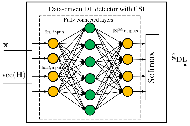
Fig. 1: Network structures for the data-driven DL detectors with CSI and without CSI.

The data-driven DL detector derived in (30) is model independent and requires no CSI to learn a detection mapping approaching MAP performance. However, it is only applicable when the channel is static and it does not perform well for varying channels [22]. Next, we will show the necessity of CSI for DL-based MIMO detection to generalize over the whole distribution of 𝐇\mathbf{H}.

From (44), the data-driven detector takes the posterior probability, po​(𝐮|𝐱)p_{o}(\mathbf{u}|\mathbf{x}), as the target and we have

po​(𝐮|𝐱)=po​(𝐮|𝐟nlr​(𝐇𝐬+𝐧))\displaystyle p_{o}(\mathbf{u}|\mathbf{x})=p_{o}(\mathbf{u}|\mathbf{f}_{\mathrm{nlr}}(\mathbf{H}\mathbf{s}+\mathbf{n})) (45)

and

po​(𝐮|𝐱)=po​(𝐮|(𝐇𝐟nlt​(𝐬)+𝐧))\displaystyle p_{o}(\mathbf{u}|\mathbf{x})=p_{o}(\mathbf{u}|(\mathbf{H}\mathbf{f}_{\mathrm{nlt}}(\mathbf{s})+\mathbf{n})) (46)

according to (7) and (8), respectively. To exploit 𝐬DL\mathbf{s}_{\mathrm{DL}} in different scenarios, we discuss two channel states:

  • •

    In time-invariant channels, 𝐇\mathbf{H} remains deterministic and constant during the training and detecting phases.

  • •

    In time-varying channels, 𝐇\mathbf{H} is randomly generated from a known continuous distribution and changes in each realization of one training sample.

In the time-invariant channels, channel matrices in training data and deployed environment are identical, and 𝐬\mathbf{s} can be recovered with low detection error using the minimum distance rule. In view of 𝐬DL≈𝐬MAP\mathbf{s}_{\mathrm{DL}}\approx\mathbf{s}_{\mathrm{MAP}} from Corollary 1, the performance of the data-driven DL detector without CSI is not affected by the state of 𝐇\mathbf{H} in the time-invariant channels.

In time-varying channels, channel matrices in training data and deployed environment are different due to randomness. As a consequence, p𝜽𝒵​(𝐮|𝐱)p_{\boldsymbol{\theta}_{\mathcal{Z}}}(\mathbf{u}|\mathbf{x}) learned from training data is inconsistent with the real posterior probability in the deployed environment and 𝐬\mathbf{s} is indistinguishable using the maximum likelihood (ML) rule. The data-driven DL detector is unable to decouple transmitted symbols from time-varying channels owing to a lack of CSI and using a single network without the information of 𝐇\mathbf{H} cannot generalize the entire distribution of possible channels for MIMO detection.

To alleviate the impact of time-varying channels, let us consider the case that channel 𝐇\mathbf{H} is already known. The MAP detector in (4) is converted into

𝐬MAP=arg⁡max𝐬∈𝕊2​dt​po​(𝐬|𝐇,𝐱),\displaystyle\mathbf{s}_{\mathrm{MAP}}=\arg\max_{\mathbf{s}\in\mathbb{S}^{2d_{t}}}p_{o}(\mathbf{s}|\,\mathbf{H},\mathbf{x}), (47)

where po​(𝐬|𝐇,𝐱)p_{o}(\mathbf{s}|\,\mathbf{H},\mathbf{x}) is the posterior probability of 𝐬\mathbf{s} given 𝐇\mathbf{H} and 𝐱\mathbf{x}.

To approximate the MAP detector in (47), the data-driven DL detector should take both 𝐇\mathbf{H} and 𝐱\mathbf{x} as its input and other structures of the data-driven DL detector remain the same. The network structures for the data-driven DL detectors with and without CSI are illustrated in Fig. 1. Similar to Corollary 1, we can also prove that the data-driven DL detector with CSI can well approximate the MAP detector in (47). Therefore, the data-driven DL detector manages to generalize over all possible realizations of 𝐇\mathbf{H} by incorporating CSI into the network design.

𝐑𝐞𝐦𝐚𝐫𝐤\mathbf{Remark} 6

In time-varying channels, CSI is essential to the data-driven DL detector to detect 𝐬\mathbf{s} over all possible realizations of the channel. Moreover, the data-driven DL detector with CSI is also model independent and can achieve the MAP comparable performance over various scenarios. In this situation, the data-driven DL detector tends to have a large network structure by taking 𝐇\mathbf{H} as the input and thus requires enormous train samples to converge, as shown in Theorem 2. The data-driven DL detector with CSI yields optimal accuracy but is prohibitive for large-sized MIMO systems.

IV Model-driven DL Detector

Simply implementing the DL detector in a data-driven fashion is ineffective in some practical scenarios, especially for large-sized MIMO systems. An alternative way is to integrate the model expert knowledge into the network structure and design model-driven DL detectors. Instead of using a conventional DNN, model-driven DL detectors usually associate iterative detection algorithms with DL, which can mitigate the impact of time-varying channels, accelerate the convergence, and reduce the complexity [23]. Each layer of the model-driven DL detector operates a single iteration in (6) and adds some trainable variables to enhance the detection performance.

Suppose that the MIMO channel model is linear as shown in (2) and channel 𝐇\mathbf{H} is known at the receiver. Model-driven DL detector 𝒟u\mathcal{D}_{u} is based on the iteration detector in (6) and is given by

𝐟ϑ(𝐇,𝐱)=𝒜~ϑlu∘𝒜~ϑlu−1∘⋯∘𝒜~ϑ0,\displaystyle\mathbf{f}_{\boldsymbol{\vartheta}}(\mathbf{H},\mathbf{x})=\tilde{\mathcal{A}}_{\boldsymbol{\vartheta}_{l_{u}}}\circ\tilde{\mathcal{A}}_{\boldsymbol{\vartheta}_{l_{u}-1}}\circ\cdots\circ\tilde{\mathcal{A}}_{\boldsymbol{\vartheta}_{0}}, (48)

where ϑi\boldsymbol{\vartheta}_{i} is the trainable parameter, ϑ=(ϑ0,…,ϑlu)\boldsymbol{\vartheta}=(\boldsymbol{\vartheta}_{0},\ldots,\boldsymbol{\vartheta}_{l_{u}}) is the parameter of 𝒟u\mathcal{D}_{u}, and 𝒜~ϑi\tilde{\mathcal{A}}_{\boldsymbol{\vartheta}_{i}} is the computation at the ii-th iteration that is parameterized by ϑi\boldsymbol{\vartheta}_{i} for i∈{0,…,lu}i\in\{0,\ldots,l_{u}\}. In particular, 𝒜~ϑi\tilde{\mathcal{A}}_{\boldsymbol{\vartheta}_{i}} depends on underlying iterative detection algorithm, i.e., 𝐟iter\mathbf{f}_{\mathrm{iter}} in (6). The training sample set of 𝒟u\mathcal{D}_{u} is defined by

Ω={(𝐱m,𝐇m,𝐬m)|𝐱∈ℝ2​dr,𝐇∈ℝ2​dr×2​dt,𝐬∈𝕊2​dt,m=1,…,|Ω|}.\displaystyle\Omega=\{(\mathbf{x}_{m},\mathbf{H}_{m},\mathbf{s}_{m})|\mathbf{x}\in\mathbb{R}^{2d_{r}},\mathbf{H}\in\mathbb{R}^{2d_{r}\times 2d_{t}},\mathbf{s}\in\mathbb{S}^{2d_{t}},m=1,\ldots,|\Omega|\}. (49)

Let J​(𝐟ϑ​(𝐱,𝐇))J(\mathbf{f}_{\boldsymbol{\vartheta}}(\mathbf{x},\mathbf{H})) be the non-negative loss function between 𝐟ϑ​(𝐱,𝐇)\mathbf{f}_{\boldsymbol{\vartheta}}(\mathbf{x},\mathbf{H}) and 𝐬\mathbf{s} and Θu={ϑ∈ℝd~u}\Theta_{u}=\{\boldsymbol{\vartheta}\in\mathbb{R}^{\tilde{d}_{u}}\} be the parameter set for d~u∈ℕ\tilde{d}_{u}\in\mathbb{N}.22 2 The selection of J​(𝐟ϑ​(𝐱,𝐇))J(\mathbf{f}_{\boldsymbol{\vartheta}}(\mathbf{x},\mathbf{H})) is not fixed, which may be MSE or KL divergence. The goal of 𝒟u\mathcal{D}_{u} is to optimize ϑ\boldsymbol{\vartheta} by minimizing J⁡(𝐟ϑ)J(\mathbf{f}_{\boldsymbol{\vartheta}}) within Θu\Theta_{u},

ϑo=arg⁡minϑ∈Θu⁡𝔼⁡{J⁡(𝐟ϑ​(𝐱,𝐇))}=arg⁡minϑ∈Θu​Ju​(𝐟ϑ),\displaystyle\boldsymbol{\vartheta}_{o}=\arg\min_{\boldsymbol{\vartheta}\in\Theta_{u}}\mathbb{E}\{J(\mathbf{f}_{\boldsymbol{\vartheta}}(\mathbf{x},\mathbf{H}))\}=\arg\min_{\boldsymbol{\vartheta}\in\Theta_{u}}J_{u}(\mathbf{f}_{\boldsymbol{\vartheta}}), (50)

where ϑo\boldsymbol{\vartheta}_{o} is the optimized parameter and Ju​(𝐟ϑo)J_{u}(\mathbf{f}_{\boldsymbol{\vartheta}_{o}}) has the lowest mean loss over all ϑ∈Θu\boldsymbol{\vartheta}\in\Theta_{u}.

However, it is difficult to obtain the explicit form of Ju​(𝐟ϑ)J_{u}(\mathbf{f}_{\boldsymbol{\vartheta}}) and the empirical mean

JΩ(𝐟ϑ)=1|Ω|∑(𝐱m,𝐇m,𝐡m,)∈ΩJ(𝐟ϑ(𝐱m,𝐇m))\displaystyle J_{\Omega}(\mathbf{f}_{\boldsymbol{\vartheta}})=\frac{1}{|\Omega|}\sum_{(\mathbf{x}_{m},\mathbf{H}_{m},\mathbf{h}_{m},)\in\Omega}J(\mathbf{f}_{\boldsymbol{\vartheta}}(\mathbf{x}_{m},\mathbf{H}_{m})) (51)

is typically used to optimize ϑ\boldsymbol{\vartheta} w.r.t. Ω\Omega. Denote

ϑΩ=arg⁡minϑ∈Θu​JΩ​(𝐟ϑ),\displaystyle\boldsymbol{\vartheta}_{\Omega}=\arg\min_{\boldsymbol{\vartheta}\in\Theta_{u}}J_{\Omega}(\mathbf{f}_{\boldsymbol{\vartheta}}), (52)

and

JΩ​(𝐟ϑΩ)=minϑ∈Θu⁡JΩ​(𝐟ϑΩ).\displaystyle J_{\Omega}(\mathbf{f}_{\boldsymbol{\vartheta}_{\Omega}})=\min_{\boldsymbol{\vartheta}\in\Theta_{u}}J_{\Omega}(\mathbf{f}_{\boldsymbol{\vartheta}_{\Omega}}). (53)

From (52) and (53), 𝐟ϑΩ​(𝐱,𝐇)\mathbf{f}_{\boldsymbol{\vartheta}_{\Omega}}(\mathbf{x},\mathbf{H}) is the optimal model-driven DL detector trained by Ω\Omega. Therefore, we can evaluate the performance of the model-driven DL detector by quantifying the distance between Ju​(𝐟ϑΩ)J_{u}(\mathbf{f}_{\boldsymbol{\vartheta}_{\Omega}}) and Ju​(𝐟ϑo)J_{u}(\mathbf{f}_{\boldsymbol{\vartheta}_{o}}).

For an integer C∈ℕC\in\mathbb{N} and a collection of functions 𝐟1​(𝐱,𝐇),…,𝐟C​(𝐱,𝐇)∈𝒟u\mathbf{f}_{1}(\mathbf{x},\mathbf{H}),\ldots,\mathbf{f}_{C}(\mathbf{x},\mathbf{H})\in\mathcal{D}_{u}, let Cu​(ϵ,Θu)C_{u}(\epsilon,\Theta_{u}) be the smallest value of CC such that

minj∈{1,…,C}⁡|JΩ​(𝐟ϑ)−JΩ​(𝐟j)|≤ε\displaystyle\min_{j\in\{1,\ldots,C\}}\big|J_{\Omega}(\mathbf{f}_{\boldsymbol{\vartheta}})-J_{\Omega}(\mathbf{f}_{j})\big|\leq\varepsilon (54)

for ε>0\varepsilon>0 and any 𝐟ϑ​(𝐱,𝐇)∈𝒟u\mathbf{f}_{\boldsymbol{\vartheta}}(\mathbf{x},\mathbf{H})\in\mathcal{D}_{u}. The following theorem, proved in Appendix F, shows the relationship between Ju​(𝐟ϑΩ)J_{u}(\mathbf{f}_{\boldsymbol{\vartheta}_{\Omega}}) and Ju​(𝐟ϑo)J_{u}(\mathbf{f}_{\boldsymbol{\vartheta}_{o}}).

𝐓𝐡𝐞𝐨𝐫𝐞𝐦\mathbf{Theorem} 3

For any ε>0\varepsilon>0 and δu>0\delta_{u}>0, we have

𝐏u​([Ju​(𝐟ϑΩ)−Ju​(𝐟ϑo)]>ε)≤8​exp⁡(ln⁡Cu−|Ω|​ε2512​δu)+𝐏Ω,\displaystyle\mathbf{P}_{u}([J_{u}(\mathbf{f}_{\boldsymbol{\vartheta}_{\Omega}})-J_{u}(\mathbf{f}_{\boldsymbol{\vartheta}_{o}})]>\varepsilon)\leq 8\exp\left(\ln C_{u}-\frac{|\Omega|\varepsilon^{2}}{512\delta_{u}}\right)+\mathbf{P}_{\Omega}, (55)

where 𝐏u\mathbf{P}_{u} denotes the distribution of the training samples in Ω\Omega and

𝐏Ω=𝐏u​(1|Ω|​∑m=1|Ω|[J⁡(𝐟ϑ​(𝐱m,𝐇m))]2≥δu).\displaystyle\mathbf{P}_{\Omega}=\mathbf{P}_{u}\bigg(\frac{1}{|\Omega|}\sum_{m=1}^{|\Omega|}[J(\mathbf{f}_{\boldsymbol{\vartheta}}(\mathbf{x}_{m},\mathbf{H}_{m}))]^{2}\geq\delta_{u}\bigg). (56)

In general, 1|Ω|​∑m=1|Ω|[J⁡(𝐟ϑ​(𝐱m,𝐇m))]2\frac{1}{|\Omega|}\sum_{m=1}^{|\Omega|}[J(\mathbf{f}_{\boldsymbol{\vartheta}}(\mathbf{x}_{m},\mathbf{H}_{m}))]^{2} converges to its mean value as |Ω||\Omega| increases, and |Ju​(𝐟ϑΩ)−Ju​(𝐟ϑo)||J_{u}(\mathbf{f}_{\boldsymbol{\vartheta}_{\Omega}})-J_{u}(\mathbf{f}_{\boldsymbol{\vartheta}_{o}})| also converges to zero if ln⁡Cu\ln C_{u} in (55) is finite. Therefore, 𝐟ϑΩ​(𝐱,𝐇)\mathbf{f}_{\boldsymbol{\vartheta}_{\Omega}}(\mathbf{x},\mathbf{H}), asymptotically approaches to the optimal model-driven DL detector, 𝐟ϑo​(𝐱,𝐇)\mathbf{f}_{\boldsymbol{\vartheta}_{o}}(\mathbf{x},\mathbf{H}), as the size of training data increases. Furthermore, the model-driven DL detector 𝐟ϑ​(𝐱,𝐇)\mathbf{f}_{\boldsymbol{\vartheta}}(\mathbf{x},\mathbf{H}) is equivalent to underlying iterative detection algorithm 𝐟⁡(𝐱,𝐇)\mathbf{f}(\mathbf{x},\mathbf{H}) if ϑ\boldsymbol{\vartheta} is set to be specific value so that 𝒜^ϑi=𝒜^i\hat{\mathcal{A}}_{\boldsymbol{\vartheta}_{i}}=\hat{\mathcal{A}}_{i} for i∈{0,…,lu}i\in\{0,\ldots,l_{u}\}. Hence, the performance of the model-driven DL detectors is better or at least equal to that of its underlying iterative detection algorithm, as indicated by Theorem 3.

𝐑𝐞𝐦𝐚𝐫𝐤\mathbf{Remark} 7

In general, the dimension of the parameter space of the model-driven detector, d~u\tilde{d}_{u}, is much smaller than that of the data-driven DL detector. Theorem 3 demonstrates that model-driven DL detectors require far fewer train samples to converge, making them more suitable to large-sized MIMO systems. The performance of the model-driven DL detectors is determined by underlying iterative detection algorithms, while most of these algorithms cannot guarantee the convergence to the MAP detector except under some special scenarios. Generally, there exits the performance gap between the model-driven and the data-driven DL detectors.

𝐑𝐞𝐦𝐚𝐫𝐤\mathbf{Remark} 8

The model-driven DL detectors are customized for specific MIMO systems and thus do not capture the model independent property of DL. On the other hand, the model-driven DL detectors may become unreliable and divergent where the presumptive system model mismatches the real environment, which severely limits their applications.

V Simulation Results

In this section, computer simulation is provided to verify that the data-driven DL detector asymptotically approaches to the MAP detector under linear and nonlinear MIMO systems. Moreover, simulation results shows that CSI is essential for the data-driven DL detector to achieve the MAP comparable performance over the time-varying channels. Moreover, simulation results demonstrate that the underlying iterative detection algorithm is the determinant factor that affects the performance of the model-driven DL detector.

V-A Simulation Setting

The SNR is defined as

SNR=𝔼​‖𝐇𝐬‖22𝔼​‖𝐧‖22.\displaystyle\mathrm{SNR}=\frac{\mathbb{E}\|\mathbf{H}\mathbf{s}\|_{2}^{2}}{\mathbb{E}\|\mathbf{n}\|_{2}^{2}}. (57)

The network of the data-driven DL detector has 44 layers and each hidden layer is equipped with the same number of neurons. Denote d~\tilde{d} as the width of the data-driven DL detector and d~=100\tilde{d}=100. We consider QPSK constellation and all transmitted symbols are generated with equal probability.

For data-driven DL detector, the simulation results are evaluated under the FC and VC cases, respectively. Unless stated otherwise, we train the network of the data-driven DL detector for 1,00,0001,00,000 iterations with a batch size of 2,0002,000 independently generated samples and test over 10,00010,000 samples. The MAP detector in (4) serves as the benchmark. The traditional model-based ZF, AMP, and SD algorithms are used to test against the data-driven DL detector.

Refer to caption
Fig. 2: The network structure of the SIC-Net.

The model-driven DL detector in simulation is based on the SIC algorithm, which is referred as to SIC-Net. Let 𝐩^i(q)∈ℝ|𝕊|2\hat{\mathbf{p}}_{i}^{(q)}\in\mathbb{R}^{|\mathbb{S}|^{2}} denote the estimated probability vector at the ii-th transmitted antenna for i∈{1,…,dt}i\in\{1,\ldots,d_{t}\}, where q∈{1,…,Q}q\in\{1,\ldots,Q\} is the iteration index for Q∈ℕQ\in\mathbb{N}. The jj-th entry of 𝐩^i(q)∈ℝ|𝕊|2\hat{\mathbf{p}}_{i}^{(q)}\in\mathbb{R}^{|\mathbb{S}|^{2}} is p^i,j(q)\hat{p}_{i,j}^{(q)} that presents the estimated probability of 𝐬j\mathbf{s}_{j} for j∈{1,…,|𝕊|2}j\in\{1,\ldots,|\mathbb{S}|^{2}\}. Let 𝐬i(q)\mathbf{s}_{i}^{(q)} be the estimated expected symbol at the ii-th transmitted antenna for the qq-th iteration, computed via

𝐬i(q)=τq​(∑j=1|𝕊|2𝐬j​p^i,j(q)+ξq​𝐬i(q−1)),\displaystyle\mathbf{s}_{i}^{(q)}=\tau_{q}\bigg(\sum_{j=1}^{|\mathbb{S}|^{2}}\mathbf{s}_{j}\hat{p}_{i,j}^{(q)}+\xi_{q}\mathbf{s}_{i}^{(q-1)}\bigg), (58)

where τq\tau_{q} and ξq\xi_{q} are trainable variables. Other settings are the same as the SIC algorithm in [9] and the corresponding network structure is illustrated in Fig. 2. The performance of SIC-Net is evaluated in linear Gaussian MIMO channels. We train SIC-Net with a relatively small 5,0005,000 samples and test over 10,00010,000 samples. The MAP detector in (4) is used as the benchmark. Other model-driven DetNet [22] and OAMP-Net [23] MIMO detectors are adopted for comparison.

V-B Linear Systems

In this subsection, we investigate the bit-error rate (BER) performance and convergence of the data-driven DL detector under a linear MIMO model in (2).

Fig. 3: The BER performance of the data-driven DL detector versus SNR compared to other MIMO detectors over the time-invariant channel.
(a) Network width
(b) Sample size
Fig. 4: The BER performance of the data-driven DL detector versus d~\tilde{d} and |𝒵||\mathcal{Z}| over the time-invariant channel, respectively.

V-B1 Time-invariant Channel

Fig. 3(a) compares the BER performance of the model-based ZF, AMP, SD, MAP and the data-driven DL detectors versus SNR where a 4×44\times 4 time-invariant correlated channel is generated according to the one-ring model in [37]. We assume that perfect CSI is available for the ZF, AMP, and SD detectors while data-driven DL detector has no CSI. Moreover, the MAP detector is evaluated under both perfect and imperfect CSI, respectively. As shown in Fig. 3, the data-driven DL detector can well approximate the MAP detector of perfect CSI and significantly outperforms other model-based detectors, which confirms that p𝜽𝒵​(𝐮|𝐱)≈po​(𝐮|𝐱)p_{\boldsymbol{\theta}_{\mathcal{Z}}}(\mathbf{u}|\mathbf{x})\approx p_{o}(\mathbf{u}|\mathbf{x}) in Corollary 1. Moreover, the MAP detector with imperfect CSI suffers from serious performance degradation. Nevertheless, the data-driven DL detector is immune to CSI uncertainty since it requires no channel information for training.

Fig. 4(a) shows the BER performance of the data-driven DL detector versus the network width, d~\tilde{d}, under fixed SNRs with the 2×22\times 2 Gaussian channel. We train the network for 400,000400,000 independently generated samples. The BERs of the MAP detectors derived at the same SNRs are used as the benchmark. The approximation error determines the BER performance of the DL estimator since |𝒵||\mathcal{Z}| is sufficiently large. When d~\tilde{d} is small, the dimension of the parameter space ΘR\Theta_{R} is not big enough to fit with po​(𝐮|𝐱)p_{o}(\mathbf{u}|\mathbf{x}). Hence, the BERs of the data-driven DL detector is significantly larger than those of the MAP detector. As d~\tilde{d} increases, the dimension of the parameter space of ΘR\Theta_{R} is enlarged and the approximation error decreases until both BERs converge, which verifies Theorem 1.

Fig. 4(b) shows the BER performance of the data-driven DL estimator versus the size of training samples, |𝒵||\mathcal{Z}|, over the 2×22\times 2 Gaussian channel. The SNRs are fixed and d~=100\tilde{d}=100. As in Fig. 4(a), the BERs of the MAP detector are used as the benchmark. Similarly, the generalization error is the main factor that affects the BER performance of the DL estimator under large d~\tilde{d}. When |𝒵||\mathcal{Z}| is small, the BERs of the data-driven DL detector do not converge and are significantly larger than those of the MAP estimator. As |𝒵||\mathcal{Z}| increases, the BERs of the data-driven DL detector gradually approach to those of the MAP detector, which verifies Theorem 2.

V-B2 Time-varying Channel

Fig. 5(a) compares the BER performance of the model-based ZF, AMP, SD, MAP and the data-driven DL detectors versus SNR over the 2×22\times 2 Gaussian channel. We assume that the ZF, AMP, and SD detectors have perfect CSI while both the DL and MAP detectors are evaluated under perfect and imperfect CSI, respectively. As illustrated in Fig. 6(a), the data-driven DL detector manages to achieve the Bayes-optimal BER performance by incorporating the perfect 𝐇\mathbf{H} in time-varying channels and outperforms the other model-based detectors substantially. Fig. 6(a) demonstrates that the data-driven DL detector can learn properly over time-varying channels. However, the BER performance of the data-driven DL detector is severely deteriorated by imperfect CSI in time-varying channels and can only approach to the MAP detector with imperfect CSI.

(a) Gaussian channel
(b) Correlated channel
Fig. 5: The BER performance of data-driven DL detector versus SNR compared to other MIMO detectors over the time-varying channel.

Fig 5(b) compares the BER performance of the model-based ZF, AMP, SD, MAP and the data-driven DL detectors versus SNR over the 2×22\times 2 correlated channel generated according to [37]. We assume that perfect CSI is available at the receiver. Fig 5(b) shows that the BER performance of the data-driven DL detector coincides with that of the MAP detector and substantially outperforms other model-based algorithms, demonstrating its ability to achieve optimal accuracy in complex environments. Fig 6(b) also indicates that the data-driven DL detector is model independent and manages to learn MAP comparable detection mapping over various channel models. Hence, the data-driven DL detector can keep the performance comparable with the MAP detector in various scenarios.

V-C Nonlinear Systems

In this subsection, we evaluate the BER performance of the data-driven DL detector under a nonlinear MIMO system. We will demonstrate that the data-driven DL detector is applicable to a broader range of scenarios than the traditional MIMO detection algorithms. Furthermore, we only compare the data-driven DL detector to the ZF and MAP detectors.

Consider a MIMO system corrupted by the quantization error of ADC. We assume that each element of the channel output undergoes an entry-wise BB bit uniform quantizer QcQ_{c}. The channel input-output model is represented by (7) and can be rewritten as

𝐱=Qc​(𝐇𝐬+𝐧).\displaystyle\mathbf{x}=Q_{c}(\mathbf{H}\mathbf{s}+\mathbf{n}). (59)

Each real-valued input of QcQ_{c} is mapped to one of 2B2^{B} bins, which are defined by the set of 2B−12^{B}-1 thresholds [r1,r2,…,r2B−1][r_{1},r_{2},\ldots,r_{2^{B}-1}] such that −∞<r−1<r2<⋯<r2B−1<∞-\infty<r-{1}<r_{2}<\cdots<r_{2^{B}-1}<\infty. Specifically, we define r0=−∞r_{0}=-\infty and r2B=∞r_{2^{B}}=\infty. The threshold rbr_{b} is given by

rb=B(−2B−1+b)2−B,forb=1,…,2B−1,\displaystyle r_{b}=\sqrt{B}(-2^{B-1}+b)2^{-B},\,\mathrm{for}\ b=1,\ldots,2^{B}-1, (60)

where the quantization output of QcQ_{c} is rb−Δ2r_{b}-\frac{\Delta}{2} when the input falls in the interval (rb−1,rb](r_{b-1},r_{b}].33 3 If b=2Bb=2^{B}, the output of QcQ_{c} is B​(−2B−1−2−1)​2−B\sqrt{B}(-2^{B-1}-2^{-1})2^{-B}.

In Fig 6, we compare the BER performance of the data-driven DL detector with the ZF and MAP detectors versus SNR over the quantized 2×22\times 2 time-varying Gaussian channel. The quantization bits are set to be 44 and 88, respectively. The perfect CSI is assumed to be available at the receiver. In Fig. 6, the BER performance of the data-driven DL detector is close to that of the MAP detector under both 55-bit and 1010-bit quantizers while the BER performance of the ZF detector degrades significantly. Hence, data-driven DL detector is also able to provide MAP comparable BER performance in quantized Gaussian channels. Fig. 6 also verifies model independence of the data-driven DL detector for nonlinear systems.

Fig. 6: The BER performance of data-driven DL detector versus SNR compared to other MIMO detectors over the quantized time-varying channel.

V-D Model-driven DL Detector

Fig. 7: The BER performance of SIC-Net versus SNR compared to other MIMO detectors over the time-varying channel.

In Fig. 7, we evaluate the BER performance of the DetNet [22], OAMP-Net [23], SIC [9], SIC-Net and MAP detectors over the 8×88\times 8 time-varying Gaussian channel. We assume that perfect CSI is available at the receiver. Fig. 7 shows that the BER performance of the SIC-Net detector is significantly better than those of the DetNet and OAMP-Net detectors but there still exits a gap between the SIC-Net and the MAP detectors, especially when SNR is high. Hence, the SIC-Net detector is suboptimal compared to the data-driven DL and MAP detectors. In Fig. 7, the BER performance of the SIC detector is close to that of the SIC-Net detector. Theorem 3 demonstrates that the SIC detector is equivalent to the optimal model-driven DL detector with the minimum Ju​(𝐟ϑ)J_{u}(\mathbf{f}_{\boldsymbol{\vartheta}}). Therefore, the performance of SIC-Net detector is determined by the SIC algorithm and the selection of detection algorithms is more important than trainable variables in improving the BER performance of the model-driven DL detectors.

VI Conclusions

In this paper, we have made the first attempt on interpreting DL-based MIMO detection with two different deep architectures: DNN embedded data-driven DL detector and iterative model-driven DL detectors. We have showed that the data-driven DL detector can converge to the MAP detector in various scenarios under suitably configured structure and sufficiently large training set. Specifically, the data-driven DL detector is robust to CSI uncertainty in time-invariant channels and suffers from imperfect CSI in time-varying channels. Moreover, the data-driven DL detector is ineffective in large-sized MIMO systems due to its requirement on a large number of training samples. On the other hand, the model-driven DL detector successfully addresses this problem by exploiting model expert knowledge and achieves relatively good performance with only a small training set since its parameter space is with a small size. However, the model-driven DL detector is suboptimal compared to the MAP detector. The strengths and weaknesses of DL-based MIMO detection should be carefully balanced when deployed in different environments.

VII Acknowledgement

Thanks for suggestions and comments from Dr. Shenglong Zhou of Imperial College London.

Appendix A Proof for Theorem 1

From (21), we have

J⁡(po)−J⁡(p𝜽)\displaystyle J(p_{o})-J(p_{\boldsymbol{\theta}}) =∑i=1dl+1∫ln⁡po​(𝐮~i|𝐱)p𝜽,i​(𝐱)​fd​e​(𝐮~i,𝐱)​𝑑𝐱=∑i=1dl+1∫g𝜽,i​(𝐱)​fd​e​(𝐮~i,𝐱)​𝑑𝐱\displaystyle=\sum_{i=1}^{d_{l+1}}\int\ln\frac{p_{o}(\tilde{\mathbf{u}}_{i}|\mathbf{x})}{p_{\boldsymbol{\theta},i}(\mathbf{x})}f_{de}(\tilde{\mathbf{u}}_{i},\mathbf{x})d\mathbf{x}=\sum_{i=1}^{d_{l+1}}\int g_{\boldsymbol{\theta},i}(\mathbf{x})f_{de}(\tilde{\mathbf{u}}_{i},\mathbf{x})d\mathbf{x} (61)

for any 𝜽∈ΘR\boldsymbol{\theta}\in\Theta_{R}, where

p𝜽,i​(𝐱)=exp⁡(f𝜽,i​(𝐱))∑j=1dl+1exp⁡(f𝜽,j​(𝐱)),\displaystyle p_{\boldsymbol{\theta},i}(\mathbf{x})=\frac{\exp(f_{\boldsymbol{\theta},i}(\mathbf{x}))}{\sum_{j=1}^{d_{l+1}}\exp(f_{\boldsymbol{\theta},j}(\mathbf{x}))}, (62)

f𝜽,i​(𝐱)f_{\boldsymbol{\theta},i}(\mathbf{x}) is the ii-th entry of 𝐟𝜽​(𝐱)\mathbf{f}_{\boldsymbol{\theta}}(\mathbf{x}), g𝜽,i​(𝐱)=ln⁡po​(𝐮~i|𝐱)p𝜽,i​(𝐱)g_{\boldsymbol{\theta},i}(\mathbf{x})=\ln\frac{p_{o}(\tilde{\mathbf{u}}_{i}|\mathbf{x})}{p_{\boldsymbol{\theta},i}(\mathbf{x})}, and fd​e​(𝐮~i,𝐱)f_{de}(\tilde{\mathbf{u}}_{i},\mathbf{x}) is joint probability density function.

Since J⁡(po)−J⁡(p𝜽)≥0J(p_{o})-J(p_{\boldsymbol{\theta}})\geq 0, we obtain

J⁡(po)−J⁡(p𝜽)\displaystyle J(p_{o})-J(p_{\boldsymbol{\theta}}) =|J⁡(po)−J⁡(p𝜽)|≤∑i=1dl+1∫|g𝜽,i​(𝐱)|​fd​e​(𝐮~i,𝐱)​𝑑𝐱.\displaystyle=|J(p_{o})-J(p_{\boldsymbol{\theta}})|\leq\sum_{i=1}^{d_{l+1}}\int|g_{\boldsymbol{\theta},i}(\mathbf{x})|f_{de}(\tilde{\mathbf{u}}_{i},\mathbf{x})d\mathbf{x}. (63)

Substituting (62) into |g𝜽,i​(𝐱)||g_{\boldsymbol{\theta},i}(\mathbf{x})| yields

|g𝜽,i​(𝐱)|=|ln⁡po​(𝐮~i|𝐱)−f𝜽,i​(𝐱)+ln⁡[∑j=1dl+1exp⁡(f𝜽,j​(𝐱))]|.\displaystyle|g_{\boldsymbol{\theta},i}(\mathbf{x})|=\bigg|\ln p_{o}(\tilde{\mathbf{u}}_{i}|\mathbf{x})-f_{\boldsymbol{\theta},i}(\mathbf{x})+\ln\bigg[\sum_{j=1}^{d_{l+1}}\exp(f_{\boldsymbol{\theta},j}(\mathbf{x}))\bigg]\bigg|. (64)

From (19), f𝜽,i​(x)f_{\boldsymbol{\theta},i}(x) is an ℝd0→ℝ\mathbb{R}^{d_{0}}\rightarrow\mathbb{R} piecewise linear function. According to [27, Theorem 2.1], any ℝd0→ℝ\mathbb{R}^{d_{0}}\rightarrow\mathbb{R} piecewise linear function can be represented by a ReLU DNN with no more than ⌈log2⁡(d0+1)⌉\lceil\log_{2}(d_{0}+1)\rceil hidden layers.

Since ln⁡po​(𝐮|𝐱)\ln p_{o}(\mathbf{u}|\mathbf{x}) has finite 2-norm for every possible 𝐮\mathbf{u}, each element of {ln⁡po​(𝐮~1|𝐱),…,ln⁡po​(𝐮~dl+1|𝐱)}\{\ln p_{o}(\tilde{\mathbf{u}}_{1}|\mathbf{x}),\ldots,\ln p_{o}(\tilde{\mathbf{u}}_{d_{l+1}}|\mathbf{x})\} can be approximated by a ReLU DNN with at most ⌈log2⁡(d0+1)⌉\lceil\log_{2}(d_{0}+1)\rceil hidden layers [27, 28]. We simply put these ReLU DNNs in parallel and combine their outputs together to compose a single ReLU DNN. As a result, there exits a DL detector with 𝜽ε∈ΘR\boldsymbol{\theta}_{\varepsilon}\in\Theta_{R} and at most ⌈log2⁡(d0+1)⌉\lceil\log_{2}(d_{0}+1)\rceil hidden layers such that

|f𝜽ε,i​(𝐱)−ln⁡po​(𝐮~i|𝐱)|≤ε\displaystyle|f_{\boldsymbol{\theta}_{\varepsilon},i}(\mathbf{x})-\ln p_{o}(\tilde{\mathbf{u}}_{i}|\mathbf{x})|\leq\varepsilon (65)

for any ε>0\varepsilon>0 and i∈{1,…,dl+1}i\in\{1,\ldots,d_{l+1}\}. From (65) and (64), |g𝜽,i​(𝐱)||g_{\boldsymbol{\theta},i}(\mathbf{x})| satisfies

|g𝜽ε,i​(𝐱)|\displaystyle|g_{\boldsymbol{\theta}_{\varepsilon},i}(\mathbf{x})| ≤|ln⁡po​(𝐮~i|𝐱)−f𝜽ε,i​(𝐱)|+|ln⁡[∑j=1dl+1exp⁡(f𝜽ε,j​(𝐱))]|≤ε+|ln⁡[∑j=1dl+1exp⁡(f𝜽ε,j​(𝐱))]|.\displaystyle\leq\big|\ln p_{o}(\tilde{\mathbf{u}}_{i}|\mathbf{x})-f_{\boldsymbol{\theta}_{\varepsilon},i}(\mathbf{x})\big|+\bigg|\ln\bigg[\sum_{j=1}^{d_{l+1}}\exp(f_{\boldsymbol{\theta}_{\varepsilon},j}(\mathbf{x}))\bigg]\bigg|\leq\varepsilon+\bigg|\ln\bigg[\sum_{j=1}^{d_{l+1}}\exp(f_{\boldsymbol{\theta}_{\varepsilon},j}(\mathbf{x}))\bigg]\bigg|. (66)

Specifically, ∑j=1dl+1exp⁡(f𝜽ε,j​(𝐱))\sum_{j=1}^{d_{l+1}}\exp(f_{\boldsymbol{\theta}_{\varepsilon},j}(\mathbf{x})) in (66) is upper bounded by

∑j=1dl+1exp⁡(f𝜽ε,j​(𝐱))≤eε​∑j=1dl+1po​(𝐮~j|𝐱)=eε\displaystyle\sum_{j=1}^{d_{l+1}}\exp(f_{\boldsymbol{\theta}_{\varepsilon},j}(\mathbf{x}))\leq e^{\varepsilon}\sum_{j=1}^{d_{l+1}}p_{o}(\tilde{\mathbf{u}}_{j}|\mathbf{x})=e^{\varepsilon} (67)

and is lower bounded by

∑j=1dl+1exp⁡(f𝜽ε,j​(𝐱))≥e−ε.\displaystyle\sum_{j=1}^{d_{l+1}}\exp(f_{\boldsymbol{\theta}_{\varepsilon},j}(\mathbf{x}))\geq e^{-\varepsilon}. (68)

Then,

|ln⁡[∑j=1dl+1exp⁡(f𝜽ε,j​(𝐱))]|≤ε\displaystyle\bigg|\ln\bigg[\sum_{j=1}^{d_{l+1}}\exp(f_{\boldsymbol{\theta}_{\varepsilon},j}(\mathbf{x}))\bigg]\bigg|\leq\varepsilon (69)

and

|g𝜽ε,i​(𝐱)|≤2​ε\displaystyle|g_{\boldsymbol{\theta}_{\varepsilon},i}(\mathbf{x})|\leq 2\varepsilon (70)

hold. Substituting (70) into (63) yields

J⁡(po)−J⁡(p𝜽ε)≤2​ε​∑i=1dl+1∫fd​e​(𝐮~i,𝐱)​𝑑𝐱=2​ε.\displaystyle J(p_{o})-J(p_{\boldsymbol{\theta}_{\varepsilon}})\leq 2\varepsilon\sum_{i=1}^{d_{l+1}}\int f_{de}(\tilde{\mathbf{u}}_{i},\mathbf{x})d\mathbf{x}=2\varepsilon. (71)

From (26), p𝜽o​(𝐮|𝐱)p_{\boldsymbol{\theta}_{o}}(\mathbf{u}|\mathbf{x}) has the lowest KL information for all 𝜽∈ΘR\boldsymbol{\theta}\in\Theta_{R} and we have

J⁡(po)−J⁡(p𝜽o)≤J⁡(po)−J⁡(p𝜽ε)≤2​ε.\displaystyle J(p_{o})-J(p_{\boldsymbol{\theta}_{o}})\leq J(p_{o})-J(p_{\boldsymbol{\theta}_{\varepsilon}})\leq 2\varepsilon. (72)

It is then easy to derive (33) from (72) since ε\varepsilon is an arbitrary positive value, which completes the proof.

Appendix B Proof for Lemma 1

According to Symmetrization Lemma in [38, Chapter II.3], the inequality in (35) holds if

𝐏⁡(|J𝒵​(p𝜽)−J⁡(p𝜽)|>ε2)≤12\displaystyle\mathbf{P}(|J_{\mathcal{Z}}(p_{\boldsymbol{\theta}})-J(p_{\boldsymbol{\theta}})|>\frac{\varepsilon}{2})\leq\frac{1}{2} (73)

for all 𝜽∈ΘR\boldsymbol{\theta}\in\Theta_{R}. Let σ2​(p𝜽)\sigma^{2}(p_{\boldsymbol{\theta}}) be the variance of ln⁡p𝜽​(𝐮|𝐱)\ln p_{\boldsymbol{\theta}}(\mathbf{u}|\mathbf{x}). Using Chebyshev’s inequality [39] yields

𝐏⁡(|J𝒵​(p𝜽)−J⁡(p𝜽)|≥ε2)≤4​σ2​(p𝜽)|𝒵|​ε2\displaystyle\mathbf{P}\big(|J_{\mathcal{Z}}(p_{\boldsymbol{\theta}})-J(p_{\boldsymbol{\theta}})|\geq\frac{\varepsilon}{2}\big)\leq\frac{4\sigma^{2}(p_{\boldsymbol{\theta}})}{|\mathcal{Z}|\varepsilon^{2}} (74)

for all 𝜽∈ΘR\boldsymbol{\theta}\in\Theta_{R}. Specifically, σ2​(p𝜽)\sigma^{2}(p_{\boldsymbol{\theta}}) satisfies

σ2​(p𝜽)\displaystyle\sigma^{2}(p_{\boldsymbol{\theta}}) =𝔼⁡{[ln⁡p𝜽​(𝐮|𝐱)]2}−J​(p𝜽)2≤𝔼⁡{[ln⁡p𝜽​(𝐮|𝐱)]2}\displaystyle=\mathbb{E}\big\{[\ln p_{\boldsymbol{\theta}}(\mathbf{u}|\mathbf{x})]^{2}\big\}-J(p_{\boldsymbol{\theta}})^{2}\leq\mathbb{E}\big\{[\ln p_{\boldsymbol{\theta}}(\mathbf{u}|\mathbf{x})]^{2}\big\}
≤∑i=1dl+1∫[|f𝜽,i​(𝐱)|+|ln⁡(∑j=1dl+1exp⁡(f𝜽,j​(𝐱)))|]2​fd​e​(𝐮~i,𝐱)​𝑑𝐱.\displaystyle\leq\sum_{i=1}^{d_{l+1}}\int\big[|f_{\boldsymbol{\theta},i}(\mathbf{x})|+\big|\ln(\sum_{j=1}^{d_{l+1}}\exp(f_{\boldsymbol{\theta},j}(\mathbf{x})))\big|\big]^{2}f_{de}(\tilde{\mathbf{u}}_{i},\mathbf{x})d\mathbf{x}. (75)

Assume that 𝒳\mathcal{X} follows the partition in (III-A) and use the fact (19). The triangle inequality assures that

|f𝜽,i​(𝐱)|\displaystyle|f_{\boldsymbol{\theta},i}(\mathbf{x})| =‖𝐰𝒳k,i​𝐱+b𝒳k,i‖2≤‖𝐰𝒳k,i‖2​‖𝐱‖2+|b𝒳k,i|\displaystyle=\|\mathbf{w}_{\mathcal{X}_{k},i}\mathbf{x}+b_{\mathcal{X}_{k},i}\|_{2}\leq\|\mathbf{w}_{\mathcal{X}_{k},i}\|_{2}\|\mathbf{x}\|_{2}+|b_{\mathcal{X}_{k},i}| (76)

for 𝐱∈𝒳k\mathbf{x}\in\mathcal{X}_{k}, where 𝐰𝒳k,i\mathbf{w}_{\mathcal{X}_{k},i} and b𝒳k,ib_{\mathcal{X}_{k},i} are the ii-th row and the ii-th entry of 𝐖𝒳k\mathbf{W}_{\mathcal{X}_{k}} and 𝐛𝒳k\mathbf{b}_{\mathcal{X}_{k}}, respectively.

From (18) and (19), ‖𝐰𝒳k,i‖2\|\mathbf{w}_{\mathcal{X}_{k},i}\|_{2} and ‖b𝒳k,i‖2\|b_{\mathcal{X}_{k},i}\|_{2} in (76) are upper bounded by

‖𝐰𝒳k,i‖2\displaystyle\|\mathbf{w}_{\mathcal{X}_{k},i}\|_{2} =‖𝐰~l,i​∏j=0l−1𝐖~j‖2=‖𝐰l,i​𝚲l​∏j=0l−1𝐖j​𝚲j‖2≤‖𝐰l,i​𝚲l‖2​∏j=0l−1‖𝐖j​𝚲j‖2≤‖𝐰l,i‖2​∏j=0l−1‖𝐖j‖2\displaystyle=\big\|\tilde{\mathbf{w}}_{l,i}\prod_{j=0}^{l-1}\tilde{\mathbf{W}}_{j}\big\|_{2}=\big\|\mathbf{w}_{l,i}\mathbf{\Lambda}_{l}\prod_{j=0}^{l-1}\mathbf{W}_{j}\mathbf{\Lambda}_{j}\big\|_{2}\leq\|\mathbf{w}_{l,i}\mathbf{\Lambda}_{l}\|_{2}\prod_{j=0}^{l-1}\big\|\mathbf{W}_{j}\mathbf{\Lambda}_{j}\big\|_{2}\leq\|\mathbf{w}_{l,i}\|_{2}\prod_{j=0}^{l-1}\big\|\mathbf{W}_{j}\big\|_{2} (77)

and

|b𝒳k,i|\displaystyle|b_{\mathcal{X}_{k},i}| =|∑j=0l−1𝐰~l,i​(∏q=0j−1𝐖~l−1−q)​𝐛l−1−j+bl,i|≤∑j=0l−1‖𝐰~l,i‖2​‖∏q=0j−1𝐖~l−1−q‖2​‖𝐛l−1−j‖2+|bl,i|\displaystyle=\Big|\sum_{j=0}^{l-1}\tilde{\mathbf{w}}_{l,i}\bigg(\prod_{q=0}^{j-1}\tilde{\mathbf{W}}_{l-1-q}\bigg)\mathbf{b}_{l-1-j}+b_{l,i}\Big|\leq\sum_{j=0}^{l-1}\|\tilde{\mathbf{w}}_{l,i}\|_{2}\big\|\prod_{q=0}^{j-1}\tilde{\mathbf{W}}_{l-1-q}\big\|_{2}\|\mathbf{b}_{l-1-j}\|_{2}+|b_{l,i}|
≤∑j=0l−1‖𝐰l,i‖2​(∏q=0j−1‖𝐖l−1−q‖2)​‖𝐛l−1−j‖2+|bl,i|,\displaystyle\leq\sum_{j=0}^{l-1}\|\mathbf{w}_{l,i}\|_{2}\bigg(\prod_{q=0}^{j-1}\|\mathbf{W}_{l-1-q}\|_{2}\bigg)\|\mathbf{b}_{l-1-j}\|_{2}+|b_{l,i}|, (78)

respectively, where 𝐰~l,i\tilde{\mathbf{w}}_{l,i} and 𝐰l,i\mathbf{w}_{l,i} are the ii-th rows of 𝐖~l\tilde{\mathbf{W}}_{l} and 𝐖l\mathbf{W}_{l} and bl,ib_{l,i} is the ii-th entry of 𝐛l\mathbf{b}_{l}. Since ‖𝐖j‖2≤R​‖𝐝‖∞=α\|\mathbf{W}_{j}\|_{2}\leq R\|\mathbf{d}\|_{\infty}=\alpha, ‖𝐛j‖2≤R​‖𝐝‖∞≤α\|\mathbf{b}_{j}\|_{2}\leq\sqrt{R}\|\mathbf{d}\|_{\infty}\leq\alpha, ‖𝐰l,i‖2≤R​‖𝐝‖∞≤α\|\mathbf{w}_{l,i}\|_{2}\leq\sqrt{R}\|\mathbf{d}\|_{\infty}\leq\alpha, and |bl,i|≤‖𝐝‖∞≤α|b_{l,i}|\leq\|\mathbf{d}\|_{\infty}\leq\alpha for j∈{0,1,…,l−1}j\in\{0,1,\ldots,l-1\}, (77) and (B) can be further bounded by

‖𝐰𝒳k,i‖2≤αl+1\displaystyle\|\mathbf{w}_{\mathcal{X}_{k},i}\|_{2}\leq\alpha^{l+1} (79)

and

|b𝒳k,i|≤(∑i=0l−1αi+1)​α+α=αl+2−αα−1≤β⁡(αl+1−1),\displaystyle|b_{\mathcal{X}_{k},i}|\leq\bigg(\sum_{i=0}^{l-1}\alpha^{i+1}\bigg)\alpha+\alpha=\frac{\alpha^{l+2}-\alpha}{\alpha-1}\leq\beta(\alpha^{l+1}-1), (80)

respectively. Substituting (76), (79), and (80) into (76) yields

|f𝜽,i​(𝐱)|\displaystyle|f_{\boldsymbol{\theta},i}(\mathbf{x})| ≤αl+1​(‖𝐱‖2+β)−β.\displaystyle\leq\alpha^{l+1}(\|\mathbf{x}\|_{2}+\beta)-\beta. (81)

Using (81), |ln⁡[∑i=1dl+1exp⁡(f𝜽,i​(𝐱))]|\big|\ln[\sum_{i=1}^{d_{l+1}}\exp(f_{\boldsymbol{\theta},i}(\mathbf{x}))]\big| in (B) is upper bounded by

|ln⁡[∑i=1dl+1exp⁡(f𝜽,i​(𝐱))]|≤ln⁡dl+1​[αl+1​(‖𝐱‖2+β)−β].\displaystyle\bigg|\ln\bigg[\sum_{i=1}^{d_{l+1}}\exp(f_{\boldsymbol{\theta},i}(\mathbf{x}))\bigg]\bigg|\leq\ln d_{l+1}\big[\alpha^{l+1}(\|\mathbf{x}\|_{2}+\beta)-\beta\big]. (82)

Combining (81) and (82), we have

σ2​(p𝜽)\displaystyle\sigma^{2}(p_{\boldsymbol{\theta}}) ≤∑i=1dl+1∫[(ln⁡dl+1+1)​(αl+1​(‖𝐱‖2+β)−β)]2​fd​e​(𝐮~i,𝐱)​𝑑𝐱\displaystyle\leq\sum_{i=1}^{d_{l+1}}\int\big[(\ln d_{l+1}+1)(\alpha^{l+1}(\|\mathbf{x}\|_{2}+\beta)-\beta)\big]^{2}f_{de}(\tilde{\mathbf{u}}_{i},\mathbf{x})d\mathbf{x}
=𝔼⁡{[(ln⁡dl+1+1)​(αl+1​(‖𝐱‖2+β)−β)]2}=ν.\displaystyle=\mathbb{E}\big\{\big[(\ln d_{l+1}+1)(\alpha^{l+1}(\|\mathbf{x}\|_{2}+\beta)-\beta)\big]^{2}\big\}=\nu. (83)

Replacing σ2​(p𝜽)\sigma^{2}(p_{\boldsymbol{\theta}}) in (74) by its bound in (B) and letting |𝒵|≥4​ν/ε2|\mathcal{Z}|\geq 4\nu/\varepsilon^{2}, we obtain the inequalities in (35) and (73), which completes the proof.

Appendix C Proof for Lemma 2

Let 𝒵i\mathcal{Z}_{i} denote the index set of training samples in 𝒵\mathcal{Z} where

𝐮j=𝐮~i,∀j∈𝒵i\displaystyle\mathbf{u}_{j}=\tilde{\mathbf{u}}_{i},\ \forall j\in\mathcal{Z}_{i} (84)

for i∈{1,…,dl+1}i\in\{1,\ldots,d_{l+1}\}. Since samples in 𝒵i\mathcal{Z}_{i} are generated according to 𝐮~i\tilde{\mathbf{u}}_{i} and (𝐮~1,…,𝐮~dl+1)(\tilde{\mathbf{u}}_{1},\ldots,\tilde{\mathbf{u}}_{d_{l+1}}) is an i.i.d. multinomial random variable, (|𝒵1|,…,|𝒵dl+1|)(|\mathcal{Z}_{1}|,\ldots,|\mathcal{Z}_{d_{l+1}}|) is also an i.i.d. multinomial random variable with probability (p⁡(𝐮~1),…,p⁡(𝐮~dl+1))(p(\tilde{\mathbf{u}}_{1}),\ldots,p(\tilde{\mathbf{u}}_{d_{l+1}})) and ∑i=1dl+1|𝒵i|=|𝒵|\sum_{i=1}^{d_{l+1}}|\mathcal{Z}_{i}|=|\mathcal{Z}|. Then, |J𝒵​(p𝜽)−J𝒵​(p𝝀)||J_{\mathcal{Z}}(p_{\boldsymbol{\theta}})-J_{\mathcal{Z}}(p_{\boldsymbol{\lambda}})| is upper bounded by

|J𝒵​(p𝜽)−J𝒵​(p𝝀)|≤1|𝒵|​∑i=1dl+1∑j∈𝒵i|ln⁡p𝜽​(𝐮j|𝐱j)−ln⁡p𝝀​(𝐮j|𝐱j)|\displaystyle|J_{\mathcal{Z}}(p_{\boldsymbol{\theta}})-J_{\mathcal{Z}}(p_{\boldsymbol{\lambda}})|\leq\frac{1}{|\mathcal{Z}|}\sum_{i=1}^{d_{l+1}}\sum_{j\in\mathcal{Z}_{i}}|\ln p_{\boldsymbol{\theta}}(\mathbf{u}_{j}|\mathbf{x}_{j})-\ln p_{\boldsymbol{\lambda}}(\mathbf{u}_{j}|\mathbf{x}_{j})|
≤1|𝒵|​∑i=1dl+1∑j∈𝒵i|f𝜽,i​(𝐱j)−f𝝀,i​(𝐱j)−ln⁡[∑i=1dl+1exp⁡(f𝜽,i​(𝐱j))]+ln⁡[∑i=1dl+1exp⁡(f𝝀,i​(𝐱j))]|\displaystyle\leq\frac{1}{|\mathcal{Z}|}\sum_{i=1}^{d_{l+1}}\sum_{j\in\mathcal{Z}_{i}}\bigg|f_{\boldsymbol{\theta},i}(\mathbf{x}_{j})-f_{\boldsymbol{\lambda},i}(\mathbf{x}_{j})-\ln\bigg[\sum_{i=1}^{d_{l+1}}\exp(f_{\boldsymbol{\theta},i}(\mathbf{x}_{j}))\bigg]+\ln\bigg[\sum_{i=1}^{d_{l+1}}\exp(f_{\boldsymbol{\lambda},i}(\mathbf{x}_{j}))\bigg]\bigg|
≤1|𝒵|​∑i=1dl+1∑j∈𝒵i|f𝜽,i​(𝐱j)−f𝝀,i​(𝐱j)|+|ln⁡[∑i=1dl+1exp⁡(f𝜽,i​(𝐱j))]−ln⁡[∑i=1dl+1exp⁡(f𝝀,i​(𝐱j))]|.\displaystyle\leq\frac{1}{|\mathcal{Z}|}\sum_{i=1}^{d_{l+1}}\sum_{j\in\mathcal{Z}_{i}}\big|f_{\boldsymbol{\theta},i}(\mathbf{x}_{j})-f_{\boldsymbol{\lambda},i}(\mathbf{x}_{j})\big|+\bigg|\ln\bigg[\sum_{i=1}^{d_{l+1}}\exp(f_{\boldsymbol{\theta},i}(\mathbf{x}_{j}))\bigg]-\ln\bigg[\sum_{i=1}^{d_{l+1}}\exp(f_{\boldsymbol{\lambda},i}(\mathbf{x}_{j}))\bigg]\bigg|. (85)

Denote 𝐕i\mathbf{V}_{i} and 𝝊i\boldsymbol{\upsilon}_{i} as the weight and the bias of the ii-th layer of 𝒟\mathcal{D} corresponding to 𝝀\boldsymbol{\lambda} for i∈{0,…,l}i\in\{0,\ldots,l\}. Let

𝜽j=(vec⁡(𝐖0),𝐛0,…,vec⁡(𝐖j−1),𝐛j−1)\displaystyle\boldsymbol{\theta}_{j}=(\mathrm{vec}(\mathbf{W}_{0}),\mathbf{b}_{0},\ldots,\mathrm{vec}(\mathbf{W}_{j-1}),\mathbf{b}_{j-1}) (86)

and

𝝀j=(vec⁡(𝐕0),𝝊0,…,vec⁡(𝐕j−1),𝝊j−1),\displaystyle\boldsymbol{\lambda}_{j}=(\mathrm{vec}(\mathbf{V}_{0}),\boldsymbol{\upsilon}_{0},\ldots,\mathrm{vec}(\mathbf{V}_{j-1}),\boldsymbol{\upsilon}_{j-1}), (87)

be the partial parameters up to the jj-th layer for j∈{1,…,l+1}j\in\{1,\ldots,l+1\}. Hence, the corresponding partial network outputs are denoted by 𝐟𝜽j​(𝐱)\mathbf{f}_{\boldsymbol{\theta}_{j}}(\mathbf{x}) and 𝐟𝝀j​(𝐱)\mathbf{f}_{\boldsymbol{\lambda}_{j}}(\mathbf{x}), respectively.

Let ej=‖𝐟𝜽j​(𝐱)−𝐟𝝀j​(𝐱)‖2e_{j}=\|\mathbf{f}_{\boldsymbol{\theta}_{j}}(\mathbf{x})-\mathbf{f}_{\boldsymbol{\lambda}_{j}}(\mathbf{x})\|_{2} be the partial error for j∈{1,…,l+1}j\in\{1,\ldots,l+1\} and el+1e_{l+1} represents |f𝜽,i​(𝐱m)−f𝝀,i​(𝐱m)|\big|f_{\boldsymbol{\theta},i}(\mathbf{x}_{m})-f_{\boldsymbol{\lambda},i}(\mathbf{x}_{m})\big| in (C). According to [28, Lemma 2] and Lemma 1, the upper bound on ej+1e_{j+1} is given by

ej+1≤r​‖𝐝‖∞​[(3​α)j​(‖𝐱‖2+1)+∑q=0j−1(3​α)q​(yj−q+1)]\displaystyle e_{j+1}\leq r\|\mathbf{d}\|_{\infty}\big[(3\alpha)^{j}(\|\mathbf{x}\|_{2}+1)+\sum_{q=0}^{j-1}(3\alpha)^{q}(y_{j-q}+1)\big] (88)

for j∈{1,…,l}j\in\{1,\ldots,l\}, where r=‖𝜽−𝝀‖∞≤2​Rr=\|\boldsymbol{\theta}-\boldsymbol{\lambda}\|_{\infty}\leq 2R and yj=αj​(‖𝐱‖2+β)−βy_{j}=\alpha^{j}(\|\mathbf{x}\|_{2}+\beta)-\beta is the upper bound on ‖𝐟𝜽j​(𝐱)‖2\|\mathbf{f}_{\boldsymbol{\theta}_{j}}(\mathbf{x})\|_{2} and ‖𝐟𝝀j​(𝐱)‖2\|\mathbf{f}_{\boldsymbol{\lambda}_{j}}(\mathbf{x})\|_{2}.

From (88), we know |f𝜽,i​(𝐱)−f𝝀,i​(𝐱)||f_{\boldsymbol{\theta},i}(\mathbf{x})-f_{\boldsymbol{\lambda},i}(\mathbf{x})| is upper bounded by

|f𝜽,i​(𝐱)−f𝝀,i​(𝐱)|\displaystyle|f_{\boldsymbol{\theta},i}(\mathbf{x})-f_{\boldsymbol{\lambda},i}(\mathbf{x})| ≤r​‖𝐝‖∞​[∑q=0l3q​αl​‖𝐱‖2+(3​α)l+∑q=0l−1[3q​αl​β−(3​α)q​(β−1)]]\displaystyle\leq r\|\mathbf{d}\|_{\infty}\bigg[\sum_{q=0}^{l}3^{q}\alpha^{l}\|\mathbf{x}\|_{2}+(3\alpha)^{l}+\sum_{q=0}^{l-1}\big[3^{q}\alpha^{l}\beta-(3\alpha)^{q}(\beta-1)\big]\bigg]
=r​‖𝐝‖∞​[3l+1−12​αl​‖𝐱‖2+(3​α)l+3l−12​αl​β−(3​α)l−13​α−1​(β−1)]\displaystyle=r\|\mathbf{d}\|_{\infty}\bigg[\frac{3^{l+1}-1}{2}\alpha^{l}\|\mathbf{x}\|_{2}+(3\alpha)^{l}+\frac{3^{l}-1}{2}\alpha^{l}\beta-\frac{(3\alpha)^{l}-1}{3\alpha-1}(\beta-1)\bigg]
≤32​r​‖𝐝‖∞​(3​α)l​(‖𝐱‖2+β)=ξ​r,\displaystyle\leq\frac{3}{2}r\|\mathbf{d}\|_{\infty}(3\alpha)^{l}(\|\mathbf{x}\|_{2}+\beta)=\xi r, (89)

where ξ=32​‖𝐝‖∞​(3​α)l​(‖𝐱‖2+β)\xi=\frac{3}{2}\|\mathbf{d}\|_{\infty}(3\alpha)^{l}(\|\mathbf{x}\|_{2}+\beta). From (C), the upper bound on ln⁡(∑i=1dl+1exp⁡(f𝜽,i​(𝐱)))\ln(\sum_{i=1}^{d_{l+1}}\exp(f_{\boldsymbol{\theta},i}(\mathbf{x}))) can be expressed as

ln⁡[∑i=1dl+1exp⁡(f𝜽,i​(𝐱))]\displaystyle\ln\bigg[\sum_{i=1}^{d_{l+1}}\exp(f_{\boldsymbol{\theta},i}(\mathbf{x}))\bigg] ≤ln[∑i=1dl+1exp(f𝝀,i(𝐱)+ξr)]=ξr+ln[∑i=1dl+1exp(f𝝀,i(𝐱)].\displaystyle\leq\ln\bigg[\sum_{i=1}^{d_{l+1}}\exp(f_{\boldsymbol{\lambda},i}(\mathbf{x})+\xi r)\bigg]=\xi r+\ln\bigg[\sum_{i=1}^{d_{l+1}}\exp(f_{\boldsymbol{\lambda},i}(\mathbf{x})\bigg]. (90)

Similarly, ln⁡[∑i=1dl+1exp⁡(f𝜽,i​(𝐱))]\ln\big[\sum_{i=1}^{d_{l+1}}\exp(f_{\boldsymbol{\theta},i}(\mathbf{x}))\big] is lower bounded by

ln⁡[∑i=1dl+1exp⁡(f𝜽,i​(𝐱))]≥ln⁡[∑i=1dl+1exp⁡(f𝝀,i​(𝐱))]−ξ​r.\displaystyle\ln\bigg[\sum_{i=1}^{d_{l+1}}\exp(f_{\boldsymbol{\theta},i}(\mathbf{x}))\bigg]\geq\ln\bigg[\sum_{i=1}^{d_{l+1}}\exp(f_{\boldsymbol{\lambda},i}(\mathbf{x}))\bigg]-\xi r. (91)

Therefore, we have

|ln⁡[∑i=1dl+1exp⁡(f𝜽,i​(𝐱))]−ln⁡[∑i=1dl+1exp⁡(f𝝀,i​(𝐱))]|≤ξ​r.\displaystyle\bigg|\ln\bigg[\sum_{i=1}^{d_{l+1}}\exp(f_{\boldsymbol{\theta},i}(\mathbf{x}))\bigg]-\ln\bigg[\sum_{i=1}^{d_{l+1}}\exp(f_{\boldsymbol{\lambda},i}(\mathbf{x}))\bigg]\bigg|\leq\xi r. (92)

Using (C) and (92), we derive the upper bound on |J𝒵​(p𝜽)−J𝒵​(p𝝀)||J_{\mathcal{Z}}(p_{\boldsymbol{\theta}})-J_{\mathcal{Z}}(p_{\boldsymbol{\lambda}})| as

|J𝒵​(p𝜽)−J𝒵​(p𝝀)|\displaystyle|J_{\mathcal{Z}}(p_{\boldsymbol{\theta}})-J_{\mathcal{Z}}(p_{\boldsymbol{\lambda}})| ≤1|𝒵|​∑m=1|𝒵|3​r​‖𝐝‖∞​(3​α)l​(‖𝐱m‖2+β)≤3l+1​‖𝐝‖∞​αl​(δ+β)​‖𝜽−𝝀‖∞,\displaystyle\leq\frac{1}{|\mathcal{Z}|}\sum_{m=1}^{|\mathcal{Z}|}3r\|\mathbf{d}\|_{\infty}(3\alpha)^{l}(\|\mathbf{x}_{m}\|_{2}+\beta)\leq 3^{l+1}\|\mathbf{d}\|_{\infty}\alpha^{l}(\delta+\beta)\|\boldsymbol{\theta}-\boldsymbol{\lambda}\|_{\infty}, (93)

which completes the proof.

Appendix D Proof for Theorem 2

From (26) and (28), we can bound J⁡(p𝜽o)−J⁡(p𝜽𝒵)J(p_{\boldsymbol{\theta}_{o}})-J(p_{\boldsymbol{\theta}_{\mathcal{Z}}}) by

0\displaystyle 0 ≤J⁡(p𝜽o)−J⁡(p𝜽𝒵)=[J⁡(p𝜽o)−J⁡(p𝜽𝒵)]−[J𝒵​(p𝜽o)−J𝒵​(p𝜽𝒵)]+[J𝒵​(p𝜽o)−J𝒵​(p𝜽𝒵)]\displaystyle\leq J(p_{\boldsymbol{\theta}_{o}})-J(p_{\boldsymbol{\theta}_{\mathcal{Z}}})=[J(p_{\boldsymbol{\theta}_{o}})-J(p_{\boldsymbol{\theta}_{\mathcal{Z}}})]-[J_{\mathcal{Z}}(p_{\boldsymbol{\theta}_{o}})-J_{\mathcal{Z}}(p_{\boldsymbol{\theta}_{\mathcal{Z}}})]+[J_{\mathcal{Z}}(p_{\boldsymbol{\theta}_{o}})-J_{\mathcal{Z}}(p_{\boldsymbol{\theta}_{\mathcal{Z}}})]
≤[J⁡(p𝜽o)−J⁡(p𝜽𝒵)]−[J𝒵​(p𝜽o)−J𝒵​(p𝜽𝒵)]≤2​sup𝜽∈ΘR|J𝒵​(p𝜽)−J⁡(p𝜽)|.\displaystyle\leq[J(p_{\boldsymbol{\theta}_{o}})-J(p_{\boldsymbol{\theta}_{\mathcal{Z}}})]-[J_{\mathcal{Z}}(p_{\boldsymbol{\theta}_{o}})-J_{\mathcal{Z}}(p_{\boldsymbol{\theta}_{\mathcal{Z}}})]\leq 2\sup_{\boldsymbol{\theta}\in\Theta_{R}}|J_{\mathcal{Z}}(p_{\boldsymbol{\theta}})-J(p_{\boldsymbol{\theta}})|. (94)

According to (D) and Lemma 1, we know the following inequalities

𝐏⁡([J⁡(p𝜽o)−J⁡(p𝜽𝒵)]>ε)\displaystyle\mathbf{P}([J(p_{\boldsymbol{\theta}_{o}})-J(p_{\boldsymbol{\theta}_{\mathcal{Z}}})]>\varepsilon) ≤𝐏⁡(sup𝜽∈ΘR|J𝒵​(p𝜽)−J⁡(p𝜽)|>ε2)≤4​𝐏​(sup𝜽∈ΘR|J𝒵∘​(p𝜽)|>ε8),\displaystyle\leq\mathbf{P}\big(\sup_{\boldsymbol{\theta}\in\Theta_{R}}|J_{\mathcal{Z}}(p_{\boldsymbol{\theta}})-J(p_{\boldsymbol{\theta}})|>\frac{\varepsilon}{2}\big)\leq 4\mathbf{P}\big(\sup_{\boldsymbol{\theta}\in\Theta_{R}}|J_{\mathcal{Z}}^{\circ}(p_{\boldsymbol{\theta}})|>\frac{\varepsilon}{8}\big), (95)

holds if |𝒵|≥16​ν/ε2|\mathcal{Z}|\geq 16\nu/\varepsilon^{2}.

Assume that 𝒵\mathcal{Z} is fixed with 1|𝒵|​∑m=1|𝒵|‖𝐱m‖22≤δ2\frac{1}{|\mathcal{Z}|}\sum_{m=1}^{|\mathcal{Z}|}\|\mathbf{x}_{m}\|_{2}^{2}\leq\delta^{2}. Let C=C⁡(ε/16,ΘR)C=C(\varepsilon/16,\Theta_{R}) and choose a collection of functions 𝐩1​(𝐱),…,𝐩C​(𝐱)∈𝒟\mathbf{p}_{1}(\mathbf{x}),\ldots,\mathbf{p}_{C}(\mathbf{x})\in\mathcal{D} such that

|J𝒵​(p𝜽)−J𝒵​(pj)|≤ε16,∀j∈{1,…,C},\displaystyle|J_{\mathcal{Z}}(p_{\boldsymbol{\theta}})-J_{\mathcal{Z}}(p_{j})|\leq\frac{\varepsilon}{16},\ \forall j\in\{1,\ldots,C\}, (96)

for any p𝜽​(𝐱)∈𝒟p_{\boldsymbol{\theta}}(\mathbf{x})\in\mathcal{D} and 𝜽∈ΘR\boldsymbol{\theta}\in\Theta_{R}. According to [28, Theorem 2], the following inequality

𝐏(sup𝜽∈ΘR|J𝒵∘(𝐟𝜽)|>ε8|𝒵)≤∑j=1C2exp[−2(|𝒵|16ε)2/∑m=1|𝒵|(2lnpj(𝐮m|𝐱m))2]\displaystyle\mathbf{P}\Big(\sup_{\boldsymbol{\theta}\in\Theta_{R}}|J_{\mathcal{Z}}^{\circ}(\mathbf{f}_{\boldsymbol{\theta}})|>\frac{\varepsilon}{8}|\mathcal{Z}\Big)\leq\sum_{j=1}^{C}2\mathrm{exp}\bigg[-2(\frac{|\mathcal{Z}|}{16}\varepsilon)^{2}/\sum_{m=1}^{|\mathcal{Z}|}(2\ln p_{j}(\mathbf{u}_{m}|\mathbf{x}_{m}))^{2}\bigg] (97)

holds. From (B) and (B), we know ∑m=1|𝒵|(ln⁡p⁡(𝐮m|𝐱m))2\sum_{m=1}^{|\mathcal{Z}|}(\ln p(\mathbf{u}_{m}|\mathbf{x}_{m}))^{2} is upper bounded by

∑m=1|𝒵|(ln⁡p⁡(𝐮m|𝐱m))2\displaystyle\sum_{m=1}^{|\mathcal{Z}|}(\ln p(\mathbf{u}_{m}|\mathbf{x}_{m}))^{2} ≤∑m=1|𝒵|[(ln⁡dl+1+1)​(αl+1​(‖𝐱m‖2+β)−β)]2\displaystyle\leq\sum_{m=1}^{|\mathcal{Z}|}\big[(\ln d_{l+1}+1)(\alpha^{l+1}(\|\mathbf{x}_{m}\|_{2}+\beta)-\beta)\big]^{2}
≤|𝒵|[(lndl+1+1)(αl+1δ+β)−β)]2=|𝒵|δ1.\displaystyle\leq|\mathcal{Z}|\big[(\ln d_{l+1}+1)(\alpha^{l+1}\delta+\beta)-\beta)\big]^{2}=|\mathcal{Z}|\delta_{\mathrm{1}}. (98)

Replacing ∑m=1|𝒵|(ln⁡p⁡(𝐮m|𝐱m))2\sum_{m=1}^{|\mathcal{Z}|}(\ln p(\mathbf{u}_{m}|\mathbf{x}_{m}))^{2} in (97) by the upper bound in (D) yields

𝐏⁡(sup𝜽∈ΘR|J𝒵∘​(𝐟𝜽)|>ε8|𝒵)≤2​e​x​p​(ln⁡C−|𝒵|​ε2512​δ1).\displaystyle\mathbf{P}\Big(\sup_{\boldsymbol{\theta}\in\Theta_{R}}|J_{\mathcal{Z}}^{\circ}(\mathbf{f}_{\boldsymbol{\theta}})|>\frac{\varepsilon}{8}|\mathcal{Z}\Big)\leq 2\mathrm{exp}\Big(\ln C-\frac{|\mathcal{Z}|\varepsilon^{2}}{512\delta_{\mathrm{1}}}\Big). (99)

According to (40), ln⁡C\ln C is upper bounded by

ln⁡C=ln⁡C⁡(ε/16,ΘR)≤ds​ln⁡[3l+1​26​αl​(δ+β)ε]≤ds​ln⁡δ2ε.\displaystyle\ln C=\ln C(\varepsilon/16,\Theta_{R})\leq d_{s}\ln\Big[\frac{3^{l+1}2^{6}\alpha^{l}(\delta+\beta)}{\varepsilon}\Big]\leq d_{s}\ln\frac{\delta_{2}}{\varepsilon}. (100)

If |𝒵|≥(1024​δ1​ds​ln⁡δ2ε)/ε2|\mathcal{Z}|\geq(1024\delta_{1}d_{s}\ln\frac{\delta_{2}}{\varepsilon})/\varepsilon^{2}, then we have ln⁡C≤|𝒵|​ε2/(1024​δ1)\ln C\leq|\mathcal{Z}|\varepsilon^{2}/(1024\delta_{1}) and

𝐏⁡(sup𝜽∈ΘR|J𝒵∘​(p𝜽)|>ε8|𝒵)≤2​e​x​p​(−|𝒵|​ε21024​δ1).\displaystyle\mathbf{P}\Big(\sup_{\boldsymbol{\theta}\in\Theta_{R}}|J_{\mathcal{Z}}^{\circ}(p_{\boldsymbol{\theta}})|>\frac{\varepsilon}{8}|\mathcal{Z}\Big)\leq 2\mathrm{exp}\Big(-\frac{|\mathcal{Z}|\varepsilon^{2}}{1024\delta_{\mathrm{1}}}\Big). (101)

Integrating out 𝐏⁡(sup𝜽∈ΘR|J𝒵∘​(p𝜽)|>ε8|𝒵)\mathbf{P}(\sup_{\boldsymbol{\theta}\in\Theta_{R}}|J_{\mathcal{Z}}^{\circ}(p_{\boldsymbol{\theta}})|>\frac{\varepsilon}{8}|\mathcal{Z}) over 𝒵\mathcal{Z} in (101) produces

𝐏⁡(sup𝜽∈ΘR|J𝒵∘​(𝐟𝜽)|>ε8)≤2​e​x​p​(−|𝒵|​ε21024​δ1)+𝐏𝒵,\displaystyle\mathbf{P}\Big(\sup_{\boldsymbol{\theta}\in\Theta_{R}}|J_{\mathcal{Z}}^{\circ}(\mathbf{f}_{\boldsymbol{\theta}})|>\frac{\varepsilon}{8}\Big)\leq 2\mathrm{exp}\Big(-\frac{|\mathcal{Z}|\varepsilon^{2}}{1024\delta_{\mathrm{1}}}\Big)+\mathbf{P}_{\mathcal{Z}}, (102)

where

𝐏𝒵=𝐏⁡(1|𝒵|​∑m=1|𝒵|‖𝐱m‖22≥δ2).\displaystyle\mathbf{P}_{\mathcal{Z}}=\mathbf{P}\Big(\frac{1}{|\mathcal{Z}|}\sum_{m=1}^{|\mathcal{Z}|}\|\mathbf{x}_{m}\|_{2}^{2}\geq\delta^{2}\Big). (103)

If δ2>μ\delta^{2}>\mu, then Chebyshev’s inequality [39] assures that

𝐏𝒵\displaystyle\mathbf{P}_{\mathcal{Z}} ≤𝐏[|1|𝒵|∑m=1|𝒵|∥𝐱m∥22−μ|≥(δ2−μ)]≤σ2|𝒵|​(δ2−μ)2.\displaystyle\leq\mathbf{P}\big[|\frac{1}{|\mathcal{Z}|}\sum_{m=1}^{|\mathcal{Z}|}\|\mathbf{x}_{m}\|_{2}^{2}-\mu|\geq(\delta^{2}-\mu)\big]\leq\frac{\sigma^{2}}{|\mathcal{Z}|(\delta^{2}-\mu)^{2}}. (104)

Combining (95) and (102), we obtain

𝐏⁡([J⁡(p𝜽o)−J⁡(p𝜽𝒵)]>ε)≤8​e​x​p​(−|𝒵|​ε21024​δ1)+4​σ2|𝒵|​(δ2−μ)2,\displaystyle\mathbf{P}([J(p_{\boldsymbol{\theta}_{o}})-J(p_{\boldsymbol{\theta}_{\mathcal{Z}}})]>\varepsilon)\leq 8\mathrm{exp}\Big(-\frac{|\mathcal{Z}|\varepsilon^{2}}{1024\delta_{\mathrm{1}}}\Big)+\frac{4\sigma^{2}}{|\mathcal{Z}|(\delta^{2}-\mu)^{2}}, (105)

which completes the proof.

Appendix E Proof for Corollary 1

According to (31), DKL​(po,p𝜽𝒵)D_{\mathrm{KL}}(p_{o},p_{\boldsymbol{\theta}_{\mathcal{Z}}}) is decomposed into the approximation and generalization errors. Theorem 1 demonstrates that there exits an optimized data-driven DL estimator 𝐩𝜽o​(𝐱)\mathbf{p}_{\boldsymbol{\theta}_{o}}(\mathbf{x}) with at most ⌈log2⁡(d0+1)⌉\lceil\log_{2}(d_{0}+1)\rceil hidden layers and sufficiently large RR such that the approximation error J⁡(p)−J⁡(p𝜽o)≤εJ(p)-J(p_{\boldsymbol{\theta}_{o}})\leq\varepsilon for any ε>0\varepsilon>0.

Moreover, Theorem 2 implies that the generalization error J⁡(p𝜽o)−J⁡(p𝜽𝒵)J(p_{\boldsymbol{\theta}_{o}})-J(p_{\boldsymbol{\theta}_{\mathcal{Z}}}) satisfies

lim|𝒵|→+∞𝐏⁡([J⁡(p𝜽o)−J⁡(p𝜽𝒵)]>ε)=0\displaystyle\lim_{|\mathcal{Z}|\rightarrow+\infty}\mathbf{P}\big([J(p_{\boldsymbol{\theta}_{o}})-J(p_{\boldsymbol{\theta}_{\mathcal{Z}}})]>\varepsilon\big)=0 (106)

for any ε>0\varepsilon>0. Combining Theorems 1 and Theorem 2, we have

lim|𝒵|→+∞𝐏⁡(DKL​(po,p𝜽𝒵)>ε)=0\displaystyle\lim_{|\mathcal{Z}|\rightarrow+\infty}\mathbf{P}\big(D_{\mathrm{KL}}(p_{o},p_{\boldsymbol{\theta}_{\mathcal{Z}}})>\varepsilon\big)=0 (107)

for any ε>0\varepsilon>0, which completes the proof.

Appendix F Proof for Theorem 3

Assume that Ω\Omega is fixed with ∑m=1|Ω|[J⁡(𝐟ϑ​(𝐱m,𝐇m))]2≥|Ω|​δu\sum_{m=1}^{|\Omega|}[J(\mathbf{f}_{\boldsymbol{\vartheta}}(\mathbf{x}_{m},\mathbf{H}_{m}))]^{2}\geq|\Omega|\delta_{u} for δu>0\delta_{u}>0, and then choose a collection of functions 𝐟1​(𝐱,𝐇),…,𝐟Cu​(𝐱,𝐇)∈𝒟u\mathbf{f}_{1}(\mathbf{x},\mathbf{H}),\ldots,\mathbf{f}_{C_{u}}(\mathbf{x},\mathbf{H})\in\mathcal{D}_{u} such that Cu=Cu​(ε/16,Θu)C_{u}=C_{u}(\varepsilon/16,\Theta_{u}). According to Hoeffding’s Inequality [39] and Theorem 2, we have

𝐏u​([Ju​(𝐟ϑΩ)−Ju​(𝐟ϑo)]>ε|Ω)\displaystyle\mathbf{P}_{u}([J_{u}(\mathbf{f}_{\boldsymbol{\vartheta}_{\Omega}})-J_{u}(\mathbf{f}_{\boldsymbol{\vartheta}_{o}})]>\varepsilon|\,\Omega) ≤∑j=1Cu8exp[−2(|Ω|16ε)2/∑m=1|Ω|(2J(𝐟j(𝐱m,𝐇m)))2]\displaystyle\leq\sum_{j=1}^{C_{u}}8\exp\bigg[-2(\frac{|\Omega|}{16}\varepsilon)^{2}/\sum_{m=1}^{|\Omega|}(2J(\mathbf{f}_{j}(\mathbf{x}_{m},\mathbf{H}_{m})))^{2}\bigg]
≤8​exp⁡(ln⁡Cu−|Ω|​ε2512​δu).\displaystyle\leq 8\exp\bigg(\ln C_{u}-\frac{|\Omega|\varepsilon^{2}}{512\delta_{u}}\bigg). (108)

Integrating out 𝐏u​([Ju​(𝐟ϑΩ)−Ju​(𝐟ϑo)]>ε|Ω)\mathbf{P}_{u}([J_{u}(\mathbf{f}_{\boldsymbol{\vartheta}_{\Omega}})-J_{u}(\mathbf{f}_{\boldsymbol{\vartheta}_{o}})]>\varepsilon|\,\Omega) over Ω\Omega yields

𝐏u​([Ju​(𝐟ϑΩ)−Ju​(𝐟ϑo)]>ε)≤8​exp⁡(ln⁡Cu−|Ω|​ε2512​δu)+𝐏Ω,\displaystyle\mathbf{P}_{u}\big([J_{u}(\mathbf{f}_{\boldsymbol{\vartheta}_{\Omega}})-J_{u}(\mathbf{f}_{\boldsymbol{\vartheta}_{o}})]>\varepsilon\big)\leq 8\exp\left(\ln C_{u}-\frac{|\Omega|\varepsilon^{2}}{512\delta_{u}}\right)+\mathbf{P}_{\Omega}, (109)

which completes the proof.

References

  • [1] T. L. Marzetta, “Noncooperative cellular wireless with unlimited numbers of base station antennas,” IEEE Trans. Wireless Commun., vol. 9, no. 11, pp. 3590–3600, Nov. 2010.
  • [2] E. G. Larsson, O. Edfors, F. Tufvesson, and T. L. Marzetta, “Massive MIMO for next generation wireless systems,” IEEE Commun. Mag., vol. 52, no. 2, pp. 186–195, Feb. 2014.
  • [3] B. Wang, F. Gao, S. Jin, H. Lin, and G. Y. Li, “Spatial- and frequency-wideband effects in millimeter-wave massive MIMO systems,” IEEE Trans. Signal Process., vol. 66, no. 13, pp. 3393–3406, 2018.
  • [4] S. Verdu, Multiuser Detection. Cambridge University Press, 1998.
  • [5] D. L. Donoho, A. Maleki, and A. Montanari, “Message-passing algorithms for compressed sensing,” Proc. Nat. Acad. Sci. USA, vol. 106, no. 45, pp. 18 914–18 919, Nov. 2009.
  • [6] M. Bayati and A. Montanari, “The dynamics of message passing on dense graphs with applications to compressed sensing,” IEEE Trans. Inf. Theory, vol. 57, no. Feb., pp. 764–785, 2011.
  • [7] R. Wang and G. B. Giannakis, “Approaching mimo channel capacity with soft detection based on hard sphere decoding,” IEEE Trans. Commun., vol. 54, no. 4, pp. 587–590, Apr. 2006.
  • [8] X.-D. Wang and H. V. Poor, “Iterative (turbo) soft interference cancellation and decoding for coded cdma,” IEEE Trans. Commun., vol. 47, no. 7, pp. 1046–1061, Jul. 1999.
  • [9] W.-J. Choi, K.-W. Cheong, and J. M. Cioffi, “Iterative soft interference cancellation for multiple antenna systems,” in Proc. IEEE Wireless Commun. Netw. Conf. Rec., Sep. 2000, pp. 304–309.
  • [10] A. Krizhevsky, I. Sutskever, and G. E. Hinton, “Imagenet classfication with deep convolutional neural networks,” in Adv. Neural Inf. Process. Syst. 25 (NeuraIPS), 2012, pp. 1097–1105.
  • [11] G. Hinton, L. Deng, D. Yu, G. Dahl, A.-R. Mohamed, N. Jaitly, A. Senior, V. Vanhoucke, P. Nguyen, B. Kingsbury et al., “Deep neural networks for acoustic modeling in speech recognition: The shared views of four research groups,” IEEE Signal Process. Mag., vol. 29, no. 6, pp. 82–97, Nov. 2012.
  • [12] Z. Qin, H. Ye, G. Y. Li, and B.-H. F. Juang, “Deep learning in physical layer communications,” IEEE Wireless Commun., vol. 26, no. 2, pp. 93–99, Apr. 2019.
  • [13] Y. Yang, F. Gao, G. Y. Li, and M. Jian, “Deep learning based downlink channel prediction for FDD massive MIMO system,” IEEE Commun. Lett., vol. 23, no. 11, Nov. 2019.
  • [14] H. Ye, L. Liang, G. Y. Li, and B.-H. F. Juang, “Deep learning-based end-to-end wireless communication systems with conditional gans as unknown channels,” IEEE Trans. Wireless Commun., vol. 19, no. 5, pp. 3133–3143, May 2020.
  • [15] T. O’Shea and J. Hoydis, “An introduction to deep learning for the physical layer,” IEEE Trans. Cogn. Commun. Netw., vol. 3, no. 4, pp. 563–575, Dec. 2017.
  • [16] H. Ye, G. Y. Li, and B.-H. F. Juang, “Deep reinforcement learning based resource allocation for V2V communications,” IEEE Trans. Veh. Technol., vol. 68, no. 4, pp. 3163–3173, Apr. 2019.
  • [17] L. Liang, H. Ye, G. Yu, and G. Y. Li, “Deep-learning-based wireless resource allocation with application to vehicular networks,” Proc. IEEE, vol. 108, no. 2, Feb. 2019.
  • [18] H. Ye, G. Y. Li, and B.-H. F. Juang, “Power of deep learning for channel estimation and signal detection in OFDM systems,” IEEE Wireless Commun. Lett., vol. 7, no. 1, pp. 114–117, Feb. 2018.
  • [19] N. Farsad and A. Goldsmith, “Neural network detection of data sequences in communication systems,” IEEE Trans. Signal Process., vol. 66, no. 21, pp. 5663–5678, Nov. 2018.
  • [20] N. Shlezinger, R. Fu, and Y. C. Eldar, “Deepsic: Deep soft interference cancellation for multiuser mimo detection,” IEEE Trans. Wireless Commun., vol. 20, no. 2, pp. 1349–1362, Feb. 2021.
  • [21] H. He, S. Jin, C.-K. Wen, F. Gao, G. Y. Li, and Z. Xu, “Model-driven deep learning for physical layer communications,” IEEE Wireless Commun., vol. 26, no. 5, Oct. 2019.
  • [22] N. Samuel, T. Diskin, and A. Wiesel, “Learning to detect,” IEEE Trans. Signal Process., vol. 67, no. 10, pp. 2554–2064, May 2019.
  • [23] H. He, C. Wen, S. Jin, and G. Y. Li, “Model-driven deep learning for MIMO detection,” IEEE Trans. Signal Process., vol. 68, pp. 1702–1715, Feb. 2020.
  • [24] G. Cybenko, “Approximation by superpositions of a sigmoidal function,” Math. Contr. Signals Syst., vol. 2, no. 4, pp. 303–314, 1989.
  • [25] K. Hornik, M. Stinchcombe, and H. White, “Multilayer feedforward networks are universal approximators,” Neural Netw., vol. 2, no. 5, pp. 359–366, 1989.
  • [26] G. F. Montúfar, R. Pascanu, K. Cho, and Y. Bengio, “On the number of linear regions of deep neural networks,” in Adv. Neural Inf. Process. Syst. 27 (NeuraIPS), Dec. 2014, pp. 2924–2932.
  • [27] R. Arora, A. Basu, P. Mianjy, and A. Mukherjee, “Understanding deep neural networks with rectified linear units,” in Int. Conf. Learning Rep. (ICLR), 2018.
  • [28] Q. Hu, F. Gao, H. Zhang, S. Jin, and G. Y. Li, “Deep learning for channel estimation: Interpretation, performance, and comparison,” IEEE Trans. Wireless Commun., vol. 20, no. 4, pp. 2398–2412, Apr. 2021.
  • [29] S. M. Kay, Fundamentals of Statistical Signal Processing. Prentice Hall PTR, 1993.
  • [30] C. Szegedy, W. Liu, Y. Jia, P. Sermanet, and A. Rabinovich, “Going deeper with convolutions,” in Proc. IEEE Conf. Comput. Vis. Pattern Recognit. (CVPR), Jun. 2015, pp. 1–9.
  • [31] K. He, X. Zhang, S. Ren, and J. Sun, “Deep residual learning for image recognition,” in Proc. IEEE Conf. Comput. Vis. Pattern Recognit. (CVPR), Jun. 2016, pp. 770–778.
  • [32] E. Costa, M. Midrio, and S. Pupolin, “Impact of amplifier nonlinearities on OFDM transmission system performance,” IEEE Commun. Lett., vol. 3, no. 2, pp. 37–39, Feb. 1999.
  • [33] E. Costa and S. Pupolin, “M-QAM-OFDM system performance in the presence of a nonlinear amplifier and phase noise,” IEEE Trans. Commun., vol. 50, no. 3, pp. 462–472, Mar. 2002.
  • [34] L. Xu, X. Lu, S. Jin, F. Gao, and Y. Zhu, “On the uplink achievable rate of massive MIMO system with low-resolution ADC and RF impairments,” IEEE Commun. Lett., vol. 23, no. 3, pp. 502–505, Mar. 2019.
  • [35] T. M. Cover, Elements of information theory. John Wiley & Sons, 1999.
  • [36] S. van de Geer, Applications of Empirical Process Theory. Cambridge University Press, 2006.
  • [37] D.-S. Shiu, G. J. Foschini, M. J. Gans, and J. M. Kahn, “Fading correlation and its effect on the capacity of multielement antenna systems,” IEEE Trans. Commun., vol. 48, no. 3, pp. 502–513, Mar. 2000.
  • [38] D. Pollard, Convergence of stochastic processes. Springer Science & Business Media, 2012.
  • [39] W. Mendenhall, R. J. Beaver, and B. M. Beaver, Introduction to Probability and Statistics. Cengage Learning, 2012.