Complete Lagrangian and Set of Feynman Rules for Scalar Leptoquarks

Andreas Crivellin Address: CERN Theory Division, CH–1211 Geneva 23, Switzerland Address: Physik-Institut, Universität Zürich, Winterthurerstrasse 190, CH-8057 Zürich, Switzerland Address: Paul Scherrer Institut, CH–5232 Villigen PSI, Switzerland Luc Schnell Corresponding author: Corresponding author.
E-mail address: schnell@mpp.mpg.de Address: Laboratoire de Physique Théorique et Hautes Énergies, LPTHE, Sorbonne Université, CNRS, 4 place Jussieu, FR-75252 Paris Cedex 05, France Address: Departement Physik, ETH Zürich, Otto-Stern-Weg 1, CH-8093 Zürich, Switzerland Address: Département de Physique, École Polytechnique, Route de Saclay, FR-91128 Palaiseau Cedex, France

Abstract

Leptoquarks (LQs) have attracted increasing attention within recent years, mainly since they can explain the flavor anomalies found in $R(D^{(*)})$ , $b\rightarrow s\ell^{+}\ell^{-}$ transitions and the anomalous magnetic moment of the muon. In this article, we lay the groundwork for further automated analyses by presenting the complete Lagrangian and the corresponding set of Feynman rules for scalar leptoquarks. This means we consider the five representations $\Phi_{1},\Phi_{\tilde{1}},\Phi_{2},\Phi_{\tilde{2}}$ and $\Phi_{3}$ and include the triple and quartic self-interactions, as well as couplings to the Standard Model (SM) fermions, gauge bosons and the Higgs. The calculations are performed using FeynRules and all model files are publicly available online at https://gitlab.com/lucschnell/SLQrules.

Keywords:

Scalar Leptoquarks , Feynman rules , FeynRules , FeynArts , MadGraph

PROGRAM SUMMARY

Program Title: SLQrules
CPC Library link to program files: (to be added by Technical Editor)
Developer’s repository link: https://gitlab.com/lucschnell/SLQrules
Code Ocean capsule: (to be added by Technical Editor)
Licensing provisions: CC By 4.0
Programming language: Mathematica, FeynRules
Nature of problem: In order to explain the deviations from SM predictions in $R(D^{(*)})$ , $b\to\ell^{+}\ell^{-}$ transitions and the muon AMM jointly, models involving multiple LQ representations are necessary. This significantly increases the number of possible interactions and creates the need for computational tools that allow for studying the phenomenology of these LQ models in an automated manner. While model files exist for each LQ representation individually [1], we are not aware of any publicly available model files that combine all scalar LQ representations as well as their self-interactions.
Solution method: We implemented the complete scalar LQ Lagrangian in a FeynRules [2] model file and provide the corresponding MOD and UFO model files. These can be imported directly in FeynArts [3] and MadGraph [4] to obtain a versatile toolbox for the study of scalar LQs.

References

[1] Doršner, Ilja, and Admir Greljo. "Leptoquark toolbox for precision collider studies." Journal of High Energy Physics 2018.5 (2018): 1-21.
[2] Alloul, Adam, et al. "FeynRules 2.0—A complete toolbox for tree-level phenomenology." Computer Physics Communications 185.8 (2014): 2250-2300.
[3] Hahn, Thomas. "Generating Feynman diagrams and amplitudes with FeynArts 3." Computer Physics Communications 140.3 (2001): 418-431.
[4] Alwall, Johan, et al. "The automated computation of tree-level and next-to-leading order differential cross sections, and their matching to parton shower simulations." Journal of High Energy Physics 2014.7 (2014): 79.

1 Introduction

Leptoquarks (LQs) are hypothetical beyond the Standard Model (BSM) particles that were first proposed in the context of Grand Unified Theories [1, 2, 3, 4]. What makes them stand out, and defines them, are their direct couplings to leptons and quarks (i.e. they convert a quark into a lepton and vice versa). LQs were first systematically classified in Ref. [5], where ten possible LQ representations under the Standard Model (SM) gauge group were found, of which five are scalar (spin 0) and five are vector (spin 1) particles. While they have received varying degrees of attention since then, LQs have undergone a renaissance in recent years. This can be attributed to the emergence of observed flavor anomalies, i.e. the deviations from the SM predictions measured in several flavour observables. In particular, $R(D^{(*)})$ [6, 7, 8, 9, 10, 11], $b\rightarrow s\ell^{+}\ell^{-}$ observables [12, 13, 14, 15, 16, 17, 18] and the muon anomalous magnetic moment $a_{\mu}$ [19, 20] deviate from their SM predictions by $>3\sigma$ [21, 22, 23, 24, 25], $>5\sigma$ [26, 27, 28, 29, 30, 31, 32, 33] and $>4.2\sigma$ [34], respectively. Recently, the authors of Ref. [35] unveiled a further $\approx 4\sigma$ tension with the SM prediction in the forward-backward asymmetry of $\bar{B}\to D^{*}\ell\nu$ . While these hints for new physics are by themselves interesting, it is intriguing to note that they all fall into a common pattern, namely lepton flavour universality violation.

Models with LQs can account for $b\to s\ell^{+}\ell^{-}$ data [36, 37, 38, 39, 40, 41, 42, 43, 44, 45, 46, 47, 48, 49, 50, 51, 52, 53, 54, 55, 56, 57, 58, 59, 60, 61, 62, 63], $R(D^{(*)})$ [36, 37, 55, 39, 40, 41, 42, 43, 64, 45, 46, 65, 47, 56, 66, 57, 49, 50, 67, 68, 69, 70, 71, 72, 54, 73, 74, 75, 76, 77, 78, 79, 80, 81, 82, 83, 84, 85, 86, 87, 88, 89, 90, 91, 92, 93, 94, 95, 59, 60, 96, 61, 97, 98, 62, 63] and/or $a_{\mu}$ [76, 99, 100, 101, 79, 68, 102, 103, 104, 105, 106, 107, 108, 109, 93, 82, 110, 111, 112, 59, 113, 60, 114, 115, 98, 62, 116, 117], making them prime NP candidates. Also the deviation in the $\bar{B}\to D^{*}\ell\nu$ forward-backward asymmetry can be explained with LQs, as was pointed out by Ref. [118]. As a result, LQs have been studied in direct searches at LHC [119, 120, 121, 122, 123, 124, 125, 126, 127, 128, 129, 130, 131, 132, 133, 134, 135], leptonic observables [136] and oblique electroweak (EW) parameters, Higgs couplings to gauge bosons [137, 138, 139, 140, 141, 142] and a wide range of low energy precision probes [135, 143, 144, 145, 146, 103, 147, 148, 149, 150, 151, 152, 153, 154, 155, 156, 157, 158, 159, 160, 161, 162, 163].

Many models that are now being proposed to explain the flavour anomalies jointly contain multiple scalar leptoquark representations [59, 60, 93, 62, 95, 164, 63, 116, 114, 165, 61, 68]. In addition to couplings of LQs to the SM fermions and gauge bosons, also interactions with the particles of the Higgs sector and between the LQs themselves are present in such a setup. In this article, we lay the groundwork for future automated LQ analyses by presenting the complete set of Feynman rules for all five scalar LQs. We include the LQ-LQ-Higgs(-Higgs), LQ-LQ-LQ(-Higgs) and LQ-LQ-LQ-LQ couplings, as well as all couplings to the SM fermions and gauge bosons. The FeynRules [166] model files as well as the corresponding MOD and UFO files are publicly available online at https://gitlab.com/lucschnell/SLQrules and can be used for automatized LQ phenomenology using FeynArts [167] or MadGraph [168].

In Sections 2 and 3, we present our conventions by defining the complete Lagrangian for the SM extended with all five scalar LQ representations. Sec. 4 gives an overview on the computational tools and in Sec. 5, the Feynman rules for the SM interactions are listed, while the ones for the scalar LQs are given in Sec. 6. A detailed description of our treatment of charge-conjugate fermions can be found in A.

2 SM Lagrangian

The SM fermions and the Higgs field transform under the $SU(3)_{c}\times SU(2)_{L}\times U(1)_{Y}$ gauge group as

\centering\begin{tabular}[]{c | c c c c c c}&$Q^{\prime}_{i}$&$u^{\prime}_{i}$&$d^{\prime}_{i}$&$L^{\prime}_{i}$&$\ell^{\prime}_{i}$&$H$\\ \hline\cr$SU(3)_{c}$&3&3&3&1&1&1\\ $SU(2)_{L}$&2&1&1&2&1&2\\ $U(1)_{Y}$&$\frac{1}{6}$&$\frac{2}{3}$&-$\frac{1}{3}$&-$\frac{1}{2}$&-1&$\frac{1}{2}$\end{tabular}\,.\@add@centering

(1)

The prime indicates that these are the weak eigenstates. With this convention, the electric charge $Q$ can be calculated via the Gell-Mann-Nishijima formula

Q=I_{3}+Y\,,

(2)

where $Y$ is the $U(1)_{Y}$ hypercharge and $I_{3}$ the third component of the weak isospin. The left-handed quarks are components of the $SU(2)_{L}$ -doublet $Q^{\prime}$ and the right-handed ones correspond to the singlets $u^{\prime},d^{\prime}$

Q^{\prime}_{i}=\begin{pmatrix}u^{\prime}_{i,L}\\ d^{\prime}_{i,L}\end{pmatrix},u^{\prime}_{i}=\left(u^{\prime}_{i,R}\right)\text{ and }d^{\prime}_{i}=\left(d^{\prime}_{i,R}\right)\,,

(3)

where $i=1,2,3$ is the flavor index. Analogous conventions hold for the leptons

L^{\prime}_{i}=\begin{pmatrix}\nu^{\prime}_{i,L}\\ \ell^{\prime}_{i,L}\end{pmatrix}\text{ and }\ell^{\prime}_{i}=\left(\ell^{\prime}_{i,R}\right)\,.

(4)

Note that right-handed neutrinos are not considered in this work. The SM Lagrangian then takes the form

\displaystyle\begin{aligned} \mathcal{L}^{\text{SM}}&=-\frac{1}{4}B^{\mu\nu}B_{\mu\nu}-\frac{1}{4}W^{I,\mu\nu}W_{I,\mu\nu}-\frac{1}{4}G^{\alpha,\mu\nu}G_{\alpha,\mu\nu}\\ &\phantom{12}+i\left(\bar{Q}_{i}^{\prime\intercal}\not{D}Q_{i}^{\prime}\right)+i\left(\bar{L}_{i}^{\prime\intercal}\not{D}L_{i}^{\prime}\right)+i\bar{u}_{i}^{\prime}\not{D}u_{i}^{\prime}+i\bar{d}_{i}^{\prime}\not{D}d_{i}^{\prime}+i\bar{\ell}_{i}^{\prime}\not{D}\ell_{i}^{\prime}\\ &\phantom{12}+\left(\left(D^{\mu}H\right)^{\dagger}D_{\mu}H\right)+\mu_{H}^{2}\left(H^{\dagger}H\right)-\lambda_{H}\left(H^{\dagger}H\right)^{2}\\ &\phantom{12}-\left(Y^{d}_{ij}\left(\bar{Q}^{\prime\intercal}_{i}H\right)d^{\prime}_{j}+Y^{\ell}_{ij}\left(\bar{L}^{\prime\intercal}_{i}H\right)\ell_{j}^{\prime}+Y^{u}_{ij}\left(\bar{Q}^{\prime\intercal}_{i}\tilde{H}\right)u_{j}^{\prime}+\text{ h.c.}\right)\\ &\phantom{12}+\mathcal{L}_{\text{gauge-fixing}}\,.\end{aligned}

(5)

We use brackets to indicate the $SU(2)_{L}$ contractions and denote the transpose of a $SU(2)_{L}$ multiplet $\Phi$ as $\Phi^{\intercal}$ . $B^{\mu\nu},W^{I,\mu\nu}$ (with $I\in\{1,2,3\}$ ) and $G^{\alpha,\mu\nu}$ (with $\alpha\in\{1,\dots,8\}$ ) are the field strength tensors

$\displaystyle B_{\mu\nu}$	$\displaystyle=\partial_{\mu}B_{\nu}-\partial_{\nu}B_{\mu}\,,$	(6)
$\displaystyle W^{I}_{\mu\nu}$	$\displaystyle=\partial_{\mu}W^{I}_{\nu}-\partial_{\nu}W^{I}_{\mu}+gf^{IJK}W_{\mu}^{J}W_{\nu}^{K}\,,$
$\displaystyle G^{\alpha}_{\mu\nu}$	$\displaystyle=\partial_{\mu}G^{\alpha}_{\nu}-\partial_{\nu}G^{\alpha}_{\mu}+gf^{\alpha\beta\gamma}W_{\mu}^{\beta}W_{\nu}^{\gamma}\,,$

where $B_{\mu},W^{I}_{\mu},G^{\alpha}_{\mu}$ are the gauge fields corresponding to $U(1)_{Y}$ , $SU(2)_{L}$ and $SU(3)_{c}$ , respectively. $f^{IJK}$ , $f^{\alpha\beta\gamma}$ denote the structure constants of $SU(2)_{L}$ , $SU(3)_{c}$ . $Y^{d}$ , $Y^{\ell}$ , $Y^{u}$ are the Yukawa couplings and $\tilde{H}\equiv i\sigma_{2}H^{\dagger}$ , where $\sigma_{2}$ is the second Pauli matrix. In our conventions, the Pauli matrices are given by

\sigma_{1}=\begin{pmatrix}0&1\\ 1&0\end{pmatrix},\,\sigma_{2}=\begin{pmatrix}0&-i\\ i&0\end{pmatrix},\,\sigma_{3}=\begin{pmatrix}1&0\\ 0&-1\end{pmatrix}\,.

(7)

The covariant derivative is defined as

D_{\mu}\phi=\partial_{\mu}\phi-ig_{1}YB_{\mu}\phi-ig_{2}\tau_{I}W^{I}_{\mu}\phi-ig_{s}T_{\alpha}G^{\alpha}_{\mu}\phi\,,

(8)

with $I\in\{1,2,3\}$ , $\alpha\in\{1,\dots,8\}$ . $\tau_{I}=\frac{\sigma_{I}}{2},T_{\alpha}=\frac{\lambda_{\alpha}}{2}$ refer to the generators of the fundamental $SU(2)_{L}$ , $SU(3)_{c}$ representations here. The gauge-fixing part $\mathcal{L}_{\text{gauge-fixing}}$ of the Lagrangian is described in Eq. (21).

Having acquired a non-zero vacuum expectation value (VEV) $v\approx 246$ GeV after spontaneous symmetry breaking, the Higgs doublet $H$ can be expanded in modes around $v$

H=\begin{pmatrix}-i\varphi^{+}\\ \frac{v+h+i\varphi_{Z}}{\sqrt{2}}\\ \end{pmatrix}\,,

(9)

where $\varphi^{+}$ and $\varphi_{Z}$ are the Goldstone bosons and $h$ the physical Higgs field with $m_{h}\approx$ $125\text{\,}\mathrm{GeV}$ . Expressed in terms of the couplings $\mu_{H},\lambda_{H}$ (see Eq. (5)), the parameters $v,m_{h}$ read

	$\displaystyle m_{h}$	$\displaystyle=\sqrt{2}\mu_{H}\,,$		(10)
	$\displaystyle v$	$\displaystyle=\dfrac{\mu_{H}}{\sqrt{\lambda_{H}}}\,.$		(10)

The non-vanishing VEV leads to mixing of the $U(1)_{Y}$ gauge boson with the neutral component of the $SU(2)_{L}$ ones

\displaystyle\begin{aligned} \begin{pmatrix}A_{\mu}\\ Z_{\mu}\end{pmatrix}&=\begin{pmatrix}\cos\theta_{w}&\sin\theta_{w}\\ -\sin\theta_{w}&\cos\theta_{w}\end{pmatrix}\begin{pmatrix}B_{\mu}\\ W^{3}_{\mu}\end{pmatrix}\,,\\ \end{aligned}

(11)

where $\theta_{w}$ is the Weinberg angle. The remaining two $SU(2)_{L}$ gauge bosons form electric charge eigenstates

\displaystyle\begin{aligned} W^{\pm}_{\mu}&=\frac{1}{\sqrt{2}}\left(W^{1}_{\mu}\mp iW^{2}_{\mu}\right)\,.\end{aligned}

(12)

In the following, $\cos\theta_{w},\sin\theta_{w}$ will be abbreviated as $c_{w},s_{w}$ . Instead of using the coupling constants $g_{1},g_{2}$ directly, we will state the Feynman rules using the electric charge $e$ . The conversion back to $g_{1},g_{2}$ is easily carried out using

\displaystyle\begin{aligned} e=c_{w}g_{1}\,,\\ e=s_{w}g_{2}\,.\end{aligned}

(13)

The masses acquired by the gauge bosons in Eqs. (11) and (12) via spontaneous symmetry breaking are

$\displaystyle m_{A}$	$\displaystyle=0\,,$	(14)
$\displaystyle m_{W}$	$\displaystyle=\frac{v}{2}\frac{e}{s_{w}}\,,$
$\displaystyle m_{Z}$	$\displaystyle=\frac{v}{2}\frac{e}{s_{w}c_{w}}\,,$

from which it becomes clear that $A_{\mu}$ corresponds to the photon. As stated above, $Y^{d},Y^{u},Y^{\ell}$ denote the Yukawa couplings of the Higgs doublet for the down-type quarks, up-type quarks and leptons, respectively. After spontaneous symmetry breaking, they yield non-diagonal mass terms in the weak basis

	$\displaystyle m^{u}_{ij}\bar{u}_{i}^{\prime}u_{j}^{\prime}=\frac{v}{\sqrt{2}}Y^{u}_{ij}\ \bar{u}^{\prime}_{i}u^{\prime}_{j}\,,$		(15)
	$\displaystyle m^{d}_{ij}\bar{d}_{i}^{\prime}d_{j}^{\prime}=\frac{v}{\sqrt{2}}Y^{d}_{ij}\ \bar{d}^{\prime}_{i}d^{\prime}_{j}\,,$
	$\displaystyle m^{\ell}_{ij}\bar{\ell}_{i}^{\prime}\ell_{j}^{\prime}=\frac{v}{\sqrt{2}}Y^{\ell}_{ij}\ \bar{\ell}^{\prime}_{i}\ell^{\prime}_{j}\,.$

These can be diagonalized by rotating the fermion fields

$\displaystyle u_{i,L}^{\prime}$	$\displaystyle\equiv U^{uL}_{ij}u_{j,L}\,,$	$\displaystyle u_{i,R}^{\prime}$	$\displaystyle\equiv U^{uR}_{ij}u_{j,R}\,,$	(16)
$\displaystyle d_{i,L}^{\prime}$	$\displaystyle\equiv U^{dL}_{ij}d_{j,L}\,,$	$\displaystyle d_{i,R}^{\prime}$	$\displaystyle\equiv U^{dR}_{ij}d_{j,R}\,,$
$\displaystyle\ell_{i,L}^{\prime}$	$\displaystyle\equiv U^{\ell L}_{ij}\ell_{j,L}\,,$	$\displaystyle\ell_{i,R}^{\prime}$	$\displaystyle\equiv U^{\ell R}_{ij}\ell_{j,R}\,,$

where $U^{uL},U^{uR},U^{dL},U^{dR}$ , $U^{\ell L},U^{\ell R}$ are unitary matrices, $u^{\prime},d^{\prime},\ell^{\prime}$ the weak eigenstates and $u,d,\ell$ the mass eigenstates. The Yukawa couplings in this new basis

$\displaystyle\hat{Y}^{u}$	$\displaystyle\equiv\left(U^{uL}\right)^{\dagger}Y^{u}U^{uR}\,,$	(17)
$\displaystyle\hat{Y}^{d}$	$\displaystyle\equiv\left(U^{dL}\right)^{\dagger}Y^{d}U^{dR}\,,$
$\displaystyle\hat{Y}^{\ell}$	$\displaystyle\equiv\left(U^{\ell L}\right)^{\dagger}Y^{\ell}U^{\ell R}\,,$

are diagonal and are related to the fermion masses by

$\displaystyle\frac{v}{\sqrt{2}}\hat{Y}^{u}$	$\displaystyle=\text{diag}(m_{u_{1}},m_{u_{2}},m_{u_{3}})\,,$	(18)
$\displaystyle\frac{v}{\sqrt{2}}\hat{Y}^{d}$	$\displaystyle=\text{diag}(m_{d_{1}},m_{d_{2}},m_{d_{3}})\,,$
$\displaystyle\frac{v}{\sqrt{2}}\hat{Y}^{\ell}$	$\displaystyle=\text{diag}(m_{\ell_{1}},m_{\ell_{2}},m_{\ell_{3}})\,.$

The unitary matrices in Eq. (16) can for the most part be absorbed into redefinitions of the fermion fields, the only remaining physical matrix being in the weak charged current for quarks, the CKM matrix $V$

	$\displaystyle\mathcal{L}^{SM}$	$\displaystyle\supset\frac{e}{\sqrt{2}s_{w}}W_{\mu}^{+}\bar{u}^{\prime}_{i,L}\gamma^{\mu}d^{\prime}_{i,L}+\text{ h.c.}$		(19)
		$\displaystyle=\frac{e}{\sqrt{2}s_{w}}W_{\mu}^{+}\bar{u}_{k,L}\gamma^{\mu}\underbrace{\left(U^{uL}\right)_{ki}^{\dagger}\left(U^{dL}\right)_{il}}_{V_{kl}}d_{l,L}+\text{ h.c.}\,.$		(19)

Without loss of generality, we can therefore assume that the relations between the weak eigenstates $u^{\prime},d^{\prime},\ell^{\prime},\nu^{\prime}$ and the mass eigenstates $u,d,\ell,\nu$ take the form

$\displaystyle u^{\prime}_{i,L}$	$\displaystyle=u_{i,L}\,,$	$\displaystyle u^{\prime}_{i,R}$	$\displaystyle=u_{i,R}\,,$	(20)
$\displaystyle d^{\prime}_{i,L}$	$\displaystyle=V_{ij}d_{j,L}\,,$	$\displaystyle d^{\prime}_{i,R}$	$\displaystyle=d_{i,R}\,,$
$\displaystyle\ell^{\prime}_{i,L}$	$\displaystyle=\ell_{i,L}\,,$	$\displaystyle\ell^{\prime}_{i,R}$	$\displaystyle=\ell_{i,R}\,,$
$\displaystyle\nu^{\prime}_{i,L}$	$\displaystyle=\nu_{i,L}\,,$

meaning that CKM elements only appear in couplings involving left-handed down-type quarks (corresponding to the up basis). Note that while this choice does not affect the SM Feynman rules, it becomes relevant in LQ interactions with SM fermions. The gauge freedoms of the SM gauge bosons are given in Ref. [169] (our conventions correspond to $\eta_{Y},\eta_{Z},\eta_{\theta},\eta_{G}=1$ and $\eta,\eta_{s},\eta_{e},\eta^{\prime}=-1$ ). They are fixed using the Fadeev-Popov prescription [170]. Working in the Feynman gauge, we add the following gauge-fixing terms, after spontaneous symmetry breaking and expressed in terms of the physical fields $A_{\mu},Z_{\mu},W_{\mu}^{\pm},G_{\mu}^{\alpha}$ and their corresponding ghost fields $c_{A},c_{Z},c_{W^{\pm}},c_{G^{\alpha}}$ , to the Lagrangian

$\displaystyle\mathcal{L}_{\text{gauge-fixing}}$	$\displaystyle=-\frac{1}{2}\left(\partial^{\mu}A_{\mu}\right)^{2}-\frac{1}{2}\left(\partial^{\mu}Z_{\mu}-m_{Z}\varphi_{Z}\right)^{2}$	(21)
	$\displaystyle-\left(\partial^{\mu}W_{\mu}^{-}+im_{W}\varphi^{-}\right)\left(\partial^{\mu}W_{\mu}^{+}-im_{W}\varphi^{+}\right)$
	$\displaystyle-\frac{1}{2}\left(\partial^{\mu}G_{\mu}^{\alpha}\right)^{2}$
	$\displaystyle+\sum_{B\in\{A,Z,W^{\pm}\}}\bigg(\bar{c}_{W^{+}}\frac{\partial(\delta F_{W^{+}})}{\partial\alpha_{B}}+\bar{c}_{W^{-}}\frac{\partial(\delta F_{W^{+}})}{\partial\alpha_{B}}$
	$\displaystyle+\bar{c}_{Z}\frac{\partial(\delta F_{Z})}{\partial\alpha_{B}}+\bar{c}_{A}\frac{\partial(\delta F_{A})}{\partial\alpha_{B}}\bigg)c_{B}$
	$\displaystyle+\sum_{\alpha,\beta=1}^{8}\bar{c}_{G^{\alpha}}\frac{\partial(\delta F_{G^{\alpha}})}{\partial\alpha_{G^{\beta}}}c_{G^{\beta}}\,.$

The explicit expressions for $\delta F_{W^{+}},\delta F_{Z},\delta F_{A},\delta F_{G^{\alpha}}$ are given in Ref. [169].

3 LQ Lagrangian

The five possible scalar LQ representations $\Phi_{1},\Phi_{\tilde{1}},\Phi_{2},\Phi_{\tilde{2}},\Phi_{3}$ transform under the $SU(3)_{c}\times SU(2)_{L}\times U(1)_{Y}$ gauge group as [5]

\centering\begin{tabular}[]{c | c c c c c}&$\Phi_{1},$&$\Phi_{\tilde{1}}$&$\Phi_{2}$&$\Phi_{\tilde{2}}$&$\Phi_{3}$\\ \hline\cr$SU(3)_{c}$&3&3&3&3&3\\ $SU(2)_{L}$&1&1&2&2&3\\ $U(1)_{Y}$&$-\frac{1}{3}$&$-\frac{4}{3}$&$\frac{7}{6}$&$\frac{1}{6}$&$-\frac{1}{3}$\end{tabular}\,.\@add@centering

(22)

Note that we adopt the convention that all scalar LQs transform in the fundamental $SU(3)_{c}$ representation. Expanding the $SU(2)_{L}$ multiplets into their components, the following electric charge eigenstates are found

\displaystyle\begin{aligned} \Phi_{1}=\left(\Phi_{1}^{-1/3}\right),\ \Phi_{\tilde{1}}=\left(\Phi_{\tilde{1}}^{-4/3}\right),\ \Phi_{2}=\begin{pmatrix}\Phi^{+5/3}_{2}\\ \Phi^{+2/3}_{2}\end{pmatrix},\ \\ \Phi_{\tilde{2}}=\begin{pmatrix}\Phi^{+2/3}_{\tilde{2}}\\ \Phi^{-1/3}_{\tilde{2}}\end{pmatrix},\ \sigma\cdot\Phi_{3}=\begin{pmatrix}\Phi_{3}^{-1/3}&\sqrt{2}\Phi_{3}^{+2/3}\\ \sqrt{2}\Phi_{3}^{-4/3}&-\Phi_{3}^{-1/3}\end{pmatrix}\,.\end{aligned}

(23)

We decompose the scalar LQ Lagrangian as

\mathcal{L}^{\text{LQ}}=\mathcal{L}_{2\Phi}+\mathcal{L}_{\text{kin}}+\mathcal{L}_{\text{f}}+\mathcal{L}_{3\Phi}+\mathcal{L}_{4\Phi}\,,

(24)

where $\mathcal{L}_{2\Phi}$ contains the LQ masses and the LQ-LQ-Higgs(-Higgs) couplings, $\mathcal{L}_{\text{kin}}$ the kinetic terms and the couplings to the SM gauge bosons, $\mathcal{L}_{\text{f}}$ the couplings to the SM fermions, $\mathcal{L}_{3\Phi}$ the LQ-LQ-LQ(-Higgs) couplings and finally $\mathcal{L}_{4\Phi}$ the LQ-LQ-LQ-LQ interaction terms. The individual parts of the Lagrangians are discussed in more detail below.

3.1 LQ Masses and Higgs Interactions ( $\mathcal{L}_{2\Phi}$ )

The LQ masses and the LQ-LQ-Higgs(-Higgs) interactions are implemented by the Lagrangian [142, 171]

$\displaystyle\mathcal{L}_{2\Phi}=$	$\displaystyle-\sum_{a=1}^{3}\big(m_{a}^{2}+Y_{a}\left(H^{\dagger}H\right)\big)\big(\Phi_{a}^{\dagger}\Phi_{a}\big)-\sum_{a=1}^{2}\big(m_{\tilde{a}}^{2}+Y_{\tilde{a}}\left(H^{\dagger}H\right)\big)\big(\Phi_{\tilde{a}}^{\dagger}\Phi_{\tilde{a}}\big)$	(25)
	$\displaystyle-Y_{22}\big(H^{\intercal}i\sigma_{2}\Phi_{2}\big)^{\dagger}\big(H^{\intercal}i\sigma_{2}\Phi_{2}\big)-Y_{\tilde{2}\tilde{2}}\big(H^{\intercal}i\sigma_{2}\Phi_{\tilde{2}}\big)^{\dagger}\big(H^{\intercal}i\sigma_{2}\Phi_{\tilde{2}}\big)$
	$\displaystyle-iY_{33}\epsilon^{IJK}\left(H^{\dagger}\sigma^{I}H\right)\Phi_{3}^{J\dagger}\Phi_{3}^{K}$
$\displaystyle\Big[$	$\displaystyle-A_{1\tilde{2}}\big(\Phi_{\tilde{2}}^{\dagger}H\big)\Phi_{1}+A_{\tilde{2}3}\big(\Phi_{\tilde{2}}^{\dagger}\left(\sigma\cdot\Phi_{3}\right)H\big)+Y_{2\tilde{2}}\big(\Phi_{2}^{\dagger}H\big)\big(H^{\intercal}i\sigma_{2}\Phi_{\tilde{2}}\big)$
	$\displaystyle+Y_{\tilde{1}3}\big(H^{\intercal}i\sigma_{2}\left(\sigma\cdot\Phi_{3}\right)^{\dagger}H\big)\Phi_{\tilde{1}}+Y_{13}\big(H^{\dagger}\left(\sigma\cdot\Phi_{3}\right)H\big)\Phi_{1}^{\dagger}+\text{h.c.}\Big]\,.$

The color indices are omitted since they just involve trivial contractions. For example, the term with $Y_{22}$ in Eq. (25) would be $-Y_{22}\left(H^{\intercal}i\sigma_{2}\Phi_{2,c_{1}}\right)^{\dagger}$ $\left(H^{\intercal}i\sigma_{2}\Phi_{2,c_{1}}\right)$ in full notation. We use the convention that couplings with mass dimension one (zero) are denoted by $A$ ( $Y$ ).

The terms in Eq. (25) lead to mixing among the LQ eigenstates of the same electric charge after EW symmetry breaking. It is therefore convenient to collect them in the electric charge eigenstate vectors

	$\displaystyle\Phi^{-1/3}$	$\displaystyle\equiv\begin{pmatrix}\Phi_{1}^{-1/3}\\ \Phi^{-1/3}_{\tilde{2}}\\ \Phi_{3}^{-1/3}\end{pmatrix}\,,$	$\displaystyle\Phi^{+2/3}$	$\displaystyle\equiv\begin{pmatrix}\Phi_{2}^{+2/3}\\ \Phi^{+2/3}_{\tilde{2}}\\ \Phi_{3}^{+2/3}\end{pmatrix}\,,$		(26)
	$\displaystyle\Phi^{-4/3}$	$\displaystyle\equiv\begin{pmatrix}\Phi_{\tilde{1}}^{-4/3}\\ \Phi^{-4/3}_{3}\end{pmatrix}\,,$	$\displaystyle\Phi^{+5/3}$	$\displaystyle\equiv\begin{pmatrix}\Phi_{2}^{+5/3}\end{pmatrix}\,.$		(26)

After spontaneous symmetry breaking, non-diagonal mass matrices $\mathbbm{M}^{q}$ in

\mathcal{L}_{2\Phi}\supset-\sum_{q\in Q}\Phi^{q}{}^{\dagger}\mathbbm{M}^{q}\Phi^{q}

(27)

are generated with $Q=\left\{-\frac{4}{3},-\frac{1}{3},+\frac{2}{3},+\frac{5}{3}\right\}$ and [142, 171, 172]

\displaystyle\begin{aligned} \mathbbm{M}^{-1/3}&=\begin{pmatrix}m_{1}^{2}+\frac{v^{2}}{2}Y_{1}&\frac{v}{\sqrt{2}}A_{1\tilde{2}}^{*}&\frac{v^{2}}{2}Y_{13}\\ \frac{v}{\sqrt{2}}A_{1\tilde{2}}&m_{\tilde{2}}^{2}+\frac{v^{2}}{2}Y_{\tilde{2}}&\frac{v}{\sqrt{2}}A_{\tilde{2}3}\\ \frac{v^{2}}{2}Y_{13}^{*}&\frac{v}{\sqrt{2}}A^{*}_{\tilde{2}3}&m_{3}^{2}+\frac{v^{2}}{2}Y_{3}\end{pmatrix}\,,\\ \mathbbm{M}^{+2/3}&=\begin{pmatrix}m_{2}^{2}+\frac{v^{2}}{2}Y_{2}&\frac{v^{2}}{2}Y_{2\tilde{2}}&0\\ \frac{v^{2}}{2}Y_{2\tilde{2}}^{*}&m_{\tilde{2}}^{2}+\frac{v^{2}}{2}\left(Y_{\tilde{2}}+Y_{\tilde{2}\tilde{2}}\right)&-vA_{\tilde{2}3}\\ 0&-vA_{\tilde{2}3}^{*}&m_{3}^{2}+\frac{v^{2}}{2}\left(Y_{3}+Y_{33}\right)\end{pmatrix}\,,\\ \mathbbm{M}^{-4/3}&=\begin{pmatrix}m_{\tilde{1}}^{2}+\frac{v^{2}}{2}Y_{\tilde{1}}&\frac{v^{2}}{\sqrt{2}}Y_{\tilde{1}3}^{*}\\ \frac{v^{2}}{\sqrt{2}}Y_{\tilde{1}3}&m_{3}^{2}+\frac{v^{2}}{2}\left(Y_{3}-Y_{33}\right)\\ \end{pmatrix}\,,\\ \mathbbm{M}^{+5/3}&=m_{2}^{2}+\frac{v^{2}}{2}\left(Y_{2}+Y_{22}\right)\,.\end{aligned}

(28)

They can be diagonalized by rotating the LQs with unitary matrices

W^{q}\Phi^{q}\equiv\hat{\Phi}^{q}\,,

(29)

in order to arrive at the physical basis with digonal mass matrices. $W^{q}$ can be calculated perturbatively to arbitrary order in $v$ [142, 173]. At $\mathcal{O}(v^{2})$ one finds

\displaystyle\begin{aligned} W^{-1/3}&\approx\begin{pmatrix}1\!-\!\frac{v^{2}|A_{1\tilde{2}}|^{2}}{4(m_{1\tilde{2}}^{2})^{2}}&\frac{vA_{1\tilde{2}}^{*}}{\sqrt{2}m_{1\tilde{2}}^{2}}&\frac{v^{2}(Y_{13}m_{1\tilde{2}}^{2}+A_{1\tilde{2}}^{*}A_{\tilde{2}3})}{2m_{13}^{2}m_{1\tilde{2}}^{2}}\\ \frac{-vA_{1\tilde{2}}}{\sqrt{2}m_{1\tilde{2}}^{2}}&1\!-\!\frac{v^{2}}{4}\left(\!\frac{|A_{1\tilde{2}}|^{2}}{(m_{1\tilde{2}}^{2})^{2}}\!+\!\frac{|A_{\tilde{2}3}|^{2}}{(m_{3\tilde{2}}^{2})^{2}}\!\right)&\frac{-vA_{\tilde{2}3}}{\sqrt{2}m_{3\tilde{2}}^{2}}\\ \frac{-v^{2}(Y_{13}^{*}(m_{3\tilde{2}}^{2})+A_{1\tilde{2}}A_{\tilde{2}3}^{*})}{2m_{13}^{2}m_{3\tilde{2}}^{2}}&\frac{vA_{\tilde{2}3}^{*}}{\sqrt{2}m_{3\tilde{2}}^{2}}&1\!-\!\frac{v^{2}|A_{\tilde{2}3}|^{2}}{4(m_{3\tilde{2}}^{2})^{2}}\end{pmatrix}\,,\\ \rule{0.0pt}{30.00005pt}W^{+2/3}&\approx\begin{pmatrix}1&\frac{v^{2}Y_{2\tilde{2}}}{2m_{2\tilde{2}}^{2}}&0\\ \frac{-v^{2}Y_{2\tilde{2}}^{*}}{2m_{2\tilde{2}}^{2}}&1\!-\!\frac{v^{2}|A_{\tilde{2}3}|^{2}}{2(m_{3\tilde{2}}^{2})^{2}}&\frac{-vA_{\tilde{2}3}}{m_{\tilde{2}3}^{2}}\\ 0&\frac{vA_{\tilde{2}3}^{*}}{m_{\tilde{2}3}^{2}}&1-\frac{v^{2}|A_{\tilde{2}3}|^{2}}{2(m_{3\tilde{2}}^{2})^{2}}\end{pmatrix}\,,\,W^{-4/3}\approx\begin{pmatrix}1&\frac{v^{2}Y_{\tilde{1}3}^{*}}{\sqrt{2}m_{\tilde{1}3}^{2}}\\ \frac{-v^{2}Y_{\tilde{1}3}}{\sqrt{2}m_{\tilde{1}3}^{2}}&1\end{pmatrix}\,,\\ W^{+5/3}&=1\,,\end{aligned}

(30)

where $m^{2}_{ab}\equiv m_{a}^{2}-m_{b}^{2}$ for $a,b\in\left\{1,\tilde{1},2,\tilde{2},3\right\}$ . The diagonal mass matrices

\hat{\mathbbm{M}}^{q}\equiv W^{q}\mathbbm{M}^{q}\left(W^{q}\right)^{\dagger}

(31)

then read [142]

$\displaystyle\hat{\mathbbm{M}}^{-1/3}$	$\displaystyle\approx\text{diag}\Bigg(m_{1}^{2}+\frac{v^{2}}{2}\left(\!Y_{1}\!-\!\frac{\|A_{1\tilde{2}}\|^{2}}{m_{\tilde{2}1}^{2}}\!\right),\,m_{\tilde{2}}^{2}+\frac{v^{2}}{2}\left(\!Y_{\tilde{2}}\!+\!\frac{\|A_{1\tilde{2}}\|^{2}}{m_{\tilde{2}1}^{2}}\!+\!\frac{\|A_{\tilde{2}3}\|^{2}}{m_{\tilde{2}3}^{2}}\!\right),\,$	(32)
	$\displaystyle m_{3}^{2}+\frac{v^{2}}{2}\left(\!Y_{3}\!-\!\frac{\|A_{\tilde{2}3}\|^{2}}{m_{\tilde{2}3}^{2}}\right)\Bigg)\,,$
$\displaystyle\hat{\mathbbm{M}}^{+2/3}$	$\displaystyle\approx\text{diag}\Bigg(m_{2}^{2}+\frac{v^{2}}{2}Y_{2},\,m_{\tilde{2}}^{2}+\frac{v^{2}}{2}\left(Y_{\tilde{2}}+\!Y_{\tilde{2}\tilde{2}}\!+\!\frac{2\|A_{\tilde{2}3}\|^{2}}{m_{\tilde{2}3}^{2}}\!\right),\,$
	$\displaystyle m_{3}^{2}+\frac{v^{2}}{2}\left(\!Y_{3}+Y_{33}\!-\!\frac{2\|A_{\tilde{2}3}\|^{2}}{m_{\tilde{2}3}^{2}}\!\right)\Bigg)\,,$
$\displaystyle\hat{\mathbbm{M}}^{-4/3}$	$\displaystyle\approx\text{diag}\left(m_{\tilde{1}}^{2}+\frac{v^{2}}{2}Y_{\tilde{1}},\,m_{3}^{2}+\frac{v^{2}}{2}\left(Y_{3}-Y_{33}\right)\right)\,,$
$\displaystyle\hat{\mathbbm{M}}^{+5/3}$	$\displaystyle=m_{2}^{2}+\frac{v^{2}}{2}\left(Y_{2}+Y_{22}\right)\,,$

up to order $v^{2}$ .

The interactions of LQs with the Higgs field $h$ are determined by

\displaystyle\begin{aligned} \mathcal{L}_{2\Phi}&\supset\phantom{+}\sum_{q\in Q}\left(\Phi^{q\dagger}\mathbb{\Gamma}^{q}\Phi^{q}\right)h+\frac{1}{2}\sum_{q\in Q}\left(\Phi^{q\dagger}\mathbb{\Lambda}^{q}\Phi^{q}\right)hh\\ &=\phantom{+}\sum_{q\in Q}\left(\hat{\Phi}^{q\dagger}\hat{\mathbb{\Gamma}}^{q}\hat{\Phi}^{q}\right)h+\frac{1}{2}\sum_{q\in Q}\left(\hat{\Phi}^{q\dagger}\hat{\mathbb{\Lambda}}^{q}\hat{\Phi}^{q}\right)hh\,,\\ \end{aligned}

(33)

with

\displaystyle\mathbb{\Gamma}^{-1/3}

\displaystyle=-v\begin{pmatrix}Y_{1}&\frac{A_{1\tilde{2}}^{*}}{\sqrt{2}v}&Y_{13}\\ \frac{A_{1\tilde{2}}}{\sqrt{2}v}&Y_{\tilde{2}}&\frac{A_{\tilde{2}3}}{\sqrt{2}v}\\ Y_{13}^{*}&\frac{A^{*}_{\tilde{2}3}}{\sqrt{2}v}&Y_{3}\end{pmatrix}\,,

\displaystyle\mathbb{\Gamma}^{+2/3}

\displaystyle=-v\begin{pmatrix}Y_{2}&Y_{2\tilde{2}}&0\\ Y^{*}_{2\tilde{2}}&Y_{\tilde{2}}+Y_{\tilde{2}\tilde{2}}&-\frac{A_{23}}{v}\\ 0&-\frac{A^{*}_{23}}{v}&Y_{3}+Y_{33}\end{pmatrix}\,,

$\displaystyle\mathbb{\Gamma}^{-4/3}$	$\displaystyle=-v\begin{pmatrix}Y_{\tilde{1}}&\sqrt{2}Y^{*}_{\tilde{1}3}\\ \sqrt{2}Y_{\tilde{1}3}&Y_{3}-Y_{33}\\ \end{pmatrix}\,,$	$\displaystyle\mathbb{\Gamma}^{+5/3}$	$\displaystyle=-v\Big(Y_{2}+Y_{22}\Big)\,,$	(34)
$\displaystyle\mathbb{\Lambda}^{-1/3}$	$\displaystyle=-\phantom{v}\begin{pmatrix}Y_{1}&0&Y_{13}\\ 0&Y_{\tilde{2}}&0\\ Y_{13}^{*}&0&Y_{3}\end{pmatrix}\,,$	$\displaystyle\mathbb{\Lambda}^{+2/3}$	$\displaystyle=-\phantom{v}\begin{pmatrix}Y_{2}&Y_{2\tilde{2}}&0\\ Y^{*}_{2\tilde{2}}&Y_{\tilde{2}}+Y_{\tilde{2}\tilde{2}}&0\\ 0&0&Y_{3}+Y_{33}\end{pmatrix}\,,$
$\displaystyle\rule{0.0pt}{30.00005pt}\mathbb{\Lambda}^{-4/3}$	$\displaystyle=-\phantom{v}\begin{pmatrix}Y_{\tilde{1}}&\sqrt{2}Y^{*}_{\tilde{1}3}\\ \sqrt{2}Y_{\tilde{1}3}&Y_{3}-Y_{33}\\ \end{pmatrix}\,,$	$\displaystyle\mathbb{\Lambda}^{+5/3}$	$\displaystyle=-\phantom{v}\Big(Y_{2}+Y_{22}\Big)\,,$

and

\displaystyle\begin{aligned} \hat{\mathbb{\Gamma}}^{q}&=W^{q}\mathbb{\Gamma}^{q}\left(W^{q}\right)^{\dagger}\text{ for }q\in Q\,,\\ \hat{\mathbb{\Lambda}}^{q}&=W^{q}\mathbb{\Lambda}^{q}\left(W^{q}\right)^{\dagger}\text{ for }q\in Q\,.\end{aligned}

(35)

The explicit expressions for these coupling matrices up to $\mathcal{O}(v^{2})$ are given in Ref. [142].

When listing the Feynman rules for interactions involving LQs of the same charge, we will have to relate the LQ label $a\in\left\{1,\tilde{1},2,\tilde{2},3\right\}$ to the position in $\Phi^{q}$ . For this we use the coefficients

n_{a}^{q}\text{ with }q\in\left\{-\frac{4}{3},-\frac{1}{3},+\frac{2}{3},+\frac{5}{3}\right\}\text{ and }a\in\{1,\tilde{1},2,\tilde{2},3\}.

(36)

Explicitly, we have

$n_{a}^{q}$	$a=1$	$a=\tilde{1}$	$a=2$	$a=\tilde{2}$	$a=3$
$q=-\frac{1}{3}$	1	0	0	2	3
$q=+\frac{2}{3}$	0	0	1	2	3
$q=-\frac{4}{3}$	0	1	0	0	2
$q=+\frac{5}{3}$	0	0	1	0	0

Whenever $q$ is clear from the context, we write $n^{q}_{a}$ as $n_{a}$ to simplify the notation.

3.2 Kinetic Terms and Interactions with SM Gauge Bosons ( $\mathcal{L}_{\text{kin}}$ )

The kinetic terms for the LQs as well as their couplings to the SM gauge bosons are presented in this section. The same conventions as for the SM are used. For the three-dimensional adjoint representation of $SU(2)_{L}$ , the $I^{\text{th}}$ generator ( $I\in\{1,2,3\}$ ) has the $3\times 3$ matrix form $(\tilde{\epsilon}_{I})_{JK}\equiv i\epsilon_{IJK}$ , where $\epsilon_{IJK}$ is the three-dimensional Levi-Civita tensor. We use the convention $\epsilon_{123}=+1$ .

	$\mathcal{L}_{\text{kin}}$	$D_{\mu}$
$\Phi_{1}$	$\left(\left(D_{\mu}\Phi_{1}\right)^{\dagger}D^{\mu}\Phi_{1}\right)$	$\partial_{\mu}+\frac{i}{3}g_{1}B_{\mu}-ig_{s}\frac{\lambda_{\alpha}}{2}G^{\alpha}_{\mu}$
$\Phi_{\tilde{1}}$	$\left(\left(D_{\mu}\Phi_{\tilde{1}}\right)^{\dagger}D^{\mu}\Phi_{\tilde{1}}\right)$	$\partial_{\mu}+\frac{4i}{3}g_{1}B_{\mu}-ig_{s}\frac{\lambda_{\alpha}}{2}G^{\alpha}_{\mu}$
$\Phi_{2}$	$\left(\left(D_{\mu}\Phi_{2}\right)^{\dagger}D^{\mu}\Phi_{2}\right)$	$\partial_{\mu}-\frac{7i}{6}g_{1}B_{\mu}-ig_{2}\frac{\sigma_{I}}{2}W_{\mu}^{I}-ig_{s}\frac{\lambda_{\alpha}}{2}G^{\alpha}_{\mu}$
$\Phi_{\tilde{2}}$	$\left(\left(D_{\mu}\Phi_{\tilde{2}}\right)^{\dagger}D^{\mu}\Phi_{\tilde{2}}\right)$	$\partial_{\mu}-\frac{i}{6}g_{1}B_{\mu}-ig_{2}\frac{\sigma_{I}}{2}W_{\mu}^{I}-ig_{s}\frac{\lambda_{\alpha}}{2}G^{\alpha}_{\mu}$
$\Phi_{3}$	$\left(\left(D_{\mu}\Phi_{3}\right)^{\dagger}D^{\mu}\Phi_{3}\right)$	$\partial_{\mu}+\frac{i}{3}g_{1}B_{\mu}-ig_{2}\tilde{\epsilon}_{I}W_{\mu}^{I}-ig_{s}\frac{\lambda_{\alpha}}{2}G^{\alpha}_{\mu}$

(37)

By definition, the $\Phi^{q}$ couple to the photon with the electric charge $q$ . The couplings to the electroweak SM gauge bosons are given by

\displaystyle\begin{aligned} \mathcal{L}_{\text{kin}}&\supset\phantom{+}i\dfrac{e}{s_{w}c_{w}}\sum_{q\in Q}\left(\Phi^{q\dagger}\mathbbm{Z}^{q}\overset{\leftrightarrow}{\partial^{\mu}}\Phi^{q}\right)Z_{\mu}\\ &\phantom{12}+i\dfrac{e}{s_{w}}\sum_{q\in Q\backslash\left\{+\frac{5}{3}\right\}}\left(\left(\Phi^{q+1}\right)^{\dagger}\mathbbm{W}_{q}^{q+1}\overset{\leftrightarrow}{\partial^{\mu}}\Phi^{q}\right)W^{+}_{\mu}\,,\end{aligned}

(38)

where $\Phi^{\dagger}\overset{\leftrightarrow}{\partial^{\mu}}\Phi\equiv\Phi^{\dagger}\partial^{\mu}\Phi-\left(\partial^{\mu}\Phi^{\dagger}\right)\Phi$ , $Q=\left\{-\frac{4}{3},-\frac{1}{3},+\frac{2}{3},+\frac{5}{3}\right\}$ and

	$\displaystyle\mathbbm{Z}^{-1/3}$	$\displaystyle=\begin{pmatrix}\dfrac{1}{3}s_{w}^{2}&0&0\\ 0&-\dfrac{1}{2}+\dfrac{1}{3}s_{w}^{2}&0\\ 0&0&\dfrac{1}{3}s_{w}^{2}\end{pmatrix}\,,$	$\displaystyle\mathbbm{Z}^{-4/3}$	$\displaystyle=\begin{pmatrix}\dfrac{4}{3}s_{w}^{2}&0\\ 0&-1+\dfrac{4}{3}s_{w}^{2}\end{pmatrix}\,,$
	$\displaystyle\mathbbm{Z}^{+2/3}$	$\displaystyle=\begin{pmatrix}-\dfrac{1}{2}-\dfrac{2}{3}s_{w}^{2}&0&0\\ 0&\dfrac{1}{2}-\dfrac{2}{3}s_{w}^{2}&0\\ 0&0&1-\dfrac{2}{3}s_{w}^{2}\end{pmatrix}\,,$	$\displaystyle\mathbbm{Z}^{+5/3}$	$\displaystyle=\left(\dfrac{1}{2}-\dfrac{5}{3}s_{w}^{2}\right)\,,$

\displaystyle\mathbbm{W}^{+2/3}_{-1/3}

\displaystyle=\begin{pmatrix}0&0&0\\ 0&1&0\\ 0&0&-\sqrt{2}\end{pmatrix}\,,

\displaystyle\mathbbm{W}^{-1/3}_{-4/3}

\displaystyle=\begin{pmatrix}0&0\\ 0&0\\ 0&\sqrt{2}\end{pmatrix}\,,

\displaystyle\mathbbm{W}^{+5/3}_{+2/3}

\displaystyle=\begin{pmatrix}1&0&0\\ \end{pmatrix}\,.

(39)

Such interactions were first considered in Ref. [174]. Expressed in the mass basis for the LQs, they take the form

\displaystyle\begin{aligned} \mathcal{L}_{\text{kin}}&\supset+i\dfrac{e}{s_{w}c_{w}}\sum_{q\in Q}\left(\hat{\Phi}^{q\dagger}\hat{\mathbbm{Z}}^{q}\overset{\leftrightarrow}{\partial^{\mu}}\hat{\Phi}^{q}\right)Z_{\mu}\\ &\phantom{12}+i\dfrac{e}{s_{w}}\sum_{q\in Q\backslash\{+\frac{5}{3}\}}\left(\left(\hat{\Phi}^{q+1}\right)^{\dagger}\hat{\mathbbm{W}}_{q}^{q+1}\overset{\leftrightarrow}{\partial^{\mu}}\hat{\Phi}^{q}\right)W^{+}_{\mu}\,.\end{aligned}

(40)

with

\displaystyle\begin{aligned} \hat{\mathbbm{Z}}^{q}&\equiv W^{q}\mathbbm{Z}^{q}\left(W^{q}\right)^{\dagger}\text{ for }q\in Q\,,\\ \hat{\mathbbm{W}}_{q}^{q+1}&\equiv W^{q+1}\mathbbm{W}_{q}^{q+1}\left(W^{q}\right)^{\dagger}\text{ for }q\in Q\backslash\left\{+\frac{5}{3}\right\}\,.\\ \end{aligned}

(41)

Explicitly, the matrices $\hat{\mathbbm{Z}}^{q},\hat{\mathbbm{W}}_{q}^{q+1}$ are given by

\displaystyle\begin{aligned} \hat{\mathbbm{Z}}^{-1/3}&\approx\begin{pmatrix}\frac{1}{3}s_{w}^{2}-\frac{v^{2}\left|A_{1\tilde{2}}\right|^{2}}{4\left(m^{2}_{1\tilde{2}}\right)^{2}}&-\frac{vA_{1\tilde{2}}^{*}}{2\sqrt{2}m_{1\tilde{2}}^{2}}&-\frac{v^{2}A_{\tilde{2}3}A^{*}_{1\tilde{2}}}{4m^{2}_{1\tilde{2}}m_{3\tilde{2}}^{2}}\\ -\frac{vA_{1\tilde{2}}}{2\sqrt{2}m_{1\tilde{2}}^{2}}&-\frac{1}{2}+\frac{1}{3}s_{w}^{2}+\frac{v^{2}}{4}\left(\frac{\left|A_{1\tilde{2}}\right|^{2}}{\left(m_{1\tilde{2}}^{2}\right)^{2}}+\frac{\left|A_{\tilde{2}3}\right|^{2}}{\left(m_{3\tilde{2}}^{2}\right)^{2}}\right)&-\frac{vA_{\tilde{2}3}}{2\sqrt{2}m_{3\tilde{2}}^{2}}\\ -\frac{v^{2}A_{1\tilde{2}}A_{\tilde{2}3}^{*}}{4m_{1\tilde{2}}^{2}m_{3\tilde{2}}^{2}}&-\frac{vA_{\tilde{2}3}^{*}}{2\sqrt{2}m_{3\tilde{2}}^{2}}&\frac{1}{3}s_{w}^{2}-\frac{v^{2}\left|A_{\tilde{2}3}\right|^{2}}{4\left(m_{3\tilde{2}}^{2}\right)^{2}}\\ \end{pmatrix}\,,\\ \rule{0.0pt}{30.00005pt}\hat{\mathbbm{Z}}^{+2/3}&\approx\begin{pmatrix}-\frac{1}{2}-\frac{2}{3}s_{w}^{2}&\frac{v^{2}Y_{2\tilde{2}}}{2m_{2\tilde{2}}^{2}}&0\\ \frac{v^{2}Y^{*}_{2\tilde{2}}}{2m_{2\tilde{2}}^{2}}&\frac{1}{2}-\frac{2}{3}s_{w}^{2}+\frac{v^{2}\left|A_{\tilde{2}3}\right|^{2}}{2\left(m_{\tilde{2}3}^{2}\right)^{2}}&-\frac{vA_{\tilde{2}3}}{2m_{\tilde{2}3}^{2}}\\ 0&-\frac{vA_{\tilde{2}3}^{*}}{2m_{\tilde{2}3}^{2}}&1-\frac{2}{3}s_{w}^{2}-\frac{v^{2}\left|A_{\tilde{2}3}\right|^{2}}{2\left(m_{\tilde{2}3}^{2}\right)^{2}}\\ \end{pmatrix}\,,\\ \rule{0.0pt}{10.00002pt}\hat{\mathbbm{Z}}^{-4/3}&\approx\begin{pmatrix}\frac{4}{3}s_{w}^{2}&-\frac{v^{2}Y_{\tilde{1}3}^{*}}{\sqrt{2}m_{\tilde{1}3}^{2}}\\ -\frac{v^{2}Y_{\tilde{1}3}}{\sqrt{2}m_{\tilde{1}3}^{2}}&-1+\frac{4}{3}s_{w}^{2}\\ \end{pmatrix}\,,~\hat{\mathbbm{Z}}^{+5/3}=\left(\frac{1}{2}-\frac{5}{3}s_{w}^{2}\right)\,,\\ \hat{\mathbbm{W}}^{+2/3}_{-1/3}&\approx\begin{pmatrix}0&\frac{v^{2}Y_{2\tilde{2}}}{2m^{2}_{2\tilde{2}}}&0\\ \frac{vA_{1\tilde{2}}}{\sqrt{2}m_{1\tilde{2}}^{2}}&1+\frac{v^{2}}{4}\left(\frac{\left|A_{\tilde{2}3}\right|^{2}}{\left(m_{\tilde{2}3}^{2}\right)^{2}}-\frac{\left|A_{1\tilde{2}}\right|^{2}}{\left(m_{1\tilde{2}}^{2}\right)^{2}}\right)&\frac{vA_{\tilde{2}3}}{\sqrt{2}m_{\tilde{2}3}^{2}}\\ \frac{v^{2}}{\sqrt{2}m_{13}^{2}}\left(\frac{A_{1\tilde{2}}A_{\tilde{2}3}^{*}}{m^{2}_{\tilde{2}3}}-Y_{13}^{*}\right)&0&-\sqrt{2}+\frac{v^{2}\left|A_{\tilde{2}3}\right|^{2}}{2\sqrt{2}\left(m_{3\tilde{2}}^{2}\right)^{2}}\\ \end{pmatrix}\,,\\ \hat{\mathbbm{W}}^{-1/3}_{-4/3}&\approx\begin{pmatrix}0&\frac{v^{2}}{\sqrt{2}m_{13}^{2}}\left(Y_{13}+\frac{A_{\tilde{2}3}A_{1\tilde{2}}^{*}}{m_{1\tilde{2}}^{2}}\right)\\ 0&\frac{vA_{\tilde{2}3}}{m_{\tilde{2}3}^{2}}\\ \frac{v^{2}Y_{\tilde{1}3}}{m_{\tilde{1}3}^{2}}&\sqrt{2}-\frac{v^{2}\left|A_{\tilde{2}3}\right|^{2}}{2\sqrt{2}\left(m_{\tilde{2}3}^{2}\right)^{2}}\end{pmatrix}\,,~\hat{\mathbbm{W}}^{+5/3}_{+2/3}\approx\begin{pmatrix}1&-\frac{v^{2}Y_{2\tilde{2}}}{2m_{2\tilde{2}}^{2}}&0\end{pmatrix}\,,\end{aligned}

(42)

up to $\mathcal{O}(v^{2})$ , where again $m^{2}_{ab}\equiv m_{a}^{2}-m_{b}^{2}$ for $a,b\in\left\{1,\tilde{1},2,\tilde{2},3\right\}$ .

3.3 Interactions with SM Fermions ( $\mathcal{L}_{\text{f}}$ )

The interactions between the five scalar LQs and the SM fermions are listed below. $Y_{a}^{AB}{}$ with $a\in\{1,\tilde{1},2,\tilde{2},3\}$ and $A,B\in\{L,R\}$ are arbitrary complex $3\times 3$ matrices coupling LQs to a quark and a lepton. $Y_{a}^{Q,AA}$ with $a\in\left\{1,\tilde{1},2,\tilde{2},3\right\}$ and $A\in\left\{L,R\right\}$ couple LQs to two quarks. $Y_{1}^{Q,LL}$ is symmetric in flavour space (i.e. $Y_{1,ij}^{Q,LL}$ = $Y_{1,ji}^{Q,LL}$ ), $Y_{\tilde{1}}^{Q,RR}$ and $Y_{3}^{Q,LL}$ are anti-symmetric and $Y_{1}^{Q,RR}$ is again an arbitrary complex matrix. We omit the color indices whenever they just involve trivial contractions.

	$\mathcal{L}_{f}$
$\Phi_{1}$	$Y_{1,ij}^{RR}\,\bar{u}^{\prime c}_{i}\ell^{\prime}_{j}\Phi_{1}^{\dagger}+Y_{1,ij}^{LL}\,\left(\bar{Q}_{i}^{\prime c\intercal}i\sigma_{2}L^{\prime}_{j}\right)\Phi_{1}^{\dagger}+\text{h.c.}$
	$Y_{1,ij}^{Q,LL}\,\left(\bar{Q}^{\prime c\intercal}_{i,c_{1}}i\sigma_{2}Q^{\prime}_{j,c_{2}}\right)\Phi_{1,c_{3}}\epsilon^{c_{1}c_{2}c_{3}}+\text{h.c.}$
	$Y_{1,ij}^{Q,RR}\bar{u}^{\prime c}_{i,c1}d^{\prime}_{j,c_{2}}\Phi_{1,c_{3}}\epsilon^{c_{1}c_{2}c_{3}}+\text{h.c.}$
$\Phi_{\tilde{1}}$	$Y^{RR}_{\tilde{1},ij}\,\bar{d}^{\prime c}_{i}\ell^{\prime}_{j}\Phi_{\tilde{1}}^{\dagger}+\text{h.c.}$
$\Phi_{\tilde{1}}$	$Y^{Q,RR}_{\tilde{1},ij}\,\bar{u}^{\prime c}_{i,c_{1}}u^{\prime}_{j,c_{2}}\Phi_{\tilde{1},c_{3}}\epsilon^{c_{1}c_{2}c_{3}}+\text{h.c.}$
$\Phi_{2}$	$Y_{2,ij}^{RL}\,\left(\Phi_{2}^{\intercal}\bar{u}^{\prime}_{i}i\sigma_{2}L^{\prime}_{j}\right)+Y_{2,ij}^{LR}\,\left(\bar{Q}^{\prime\intercal}_{i}\ell^{\prime}_{j}\Phi_{2}\right)+\text{h.c.}$
$\Phi_{\tilde{2}}$	$Y_{\tilde{2},ij}^{RL}\,\left(\Phi_{\tilde{2}}^{\intercal}\bar{d}^{\prime}_{i}i\sigma_{2}L^{\prime}_{j}\right)+\text{h.c.}$
$\Phi_{3}$	$Y_{3,ij}^{LL}\,\left(\bar{Q}^{\prime c\intercal}_{i}i\sigma_{2}\left(\sigma\cdot\Phi_{3}\right)^{\dagger}L^{\prime}_{j}\right)+\text{h.c.}$
$\Phi_{3}$	$Y^{Q,LL}_{3,ij}\,\left(\bar{Q}^{\prime c\intercal}_{i,c_{1}}i\sigma_{2}\left(\sigma\cdot\Phi_{3,c_{3}}\right)Q^{\prime}_{j,c_{2}}\right)\epsilon^{c_{1}c_{2}c_{3}}+\text{h.c.}$

(43)

Again, we use brackets to indicate the $SU(2)_{L}$ contractions. Note that we stated the Lagrangian above before EW symmetry breaking using the weak eigenstates of the fermions (indicated by the prime). When going to the mass eigenbasis (after EW symmetry breaking), CKM matrix elements enter interactions involving left-handed down-type quarks according to Eq. (20). The charge-conjugate of a fermion field $\Psi$ is denoted as $\Psi^{c}$ , where

	$\displaystyle\Psi^{c}$	$\displaystyle=C\bar{\Psi}^{\intercal}\,,$		(44)
	$\displaystyle\bar{\Psi}^{c}$	$\displaystyle=-\Psi^{\intercal}C^{-1}\,,$		(44)

with $C$ the charge conjugation matrix. A detailed description of our treatment of charge-conjugate SM fermions is given in A.

3.4 Triple LQ Interactions ( $\mathcal{L}_{3\Phi}$ )

Let us now turn to the LQ-LQ-LQ(-Higgs) interactions. In order to get a $SU(3)_{c}$ singlet, either three LQs or three anti-LQs have to be combined, since

\displaystyle\begin{aligned} 3\otimes 3\otimes 3&=1\oplus 8\oplus 8\oplus 10\\ \overline{3}\otimes\overline{3}\otimes\overline{3}&=1\oplus 8\oplus 8\oplus\overline{10}\end{aligned}

(45)

are the only tensor products of three SU(3) (anti-)triplets $3,\overline{3}$ that contain a singlet. Regarding the hypercharge $Y$ , one finds the possible combinations listed in Table 1.

		LQ Fields (and their $Y$ )
		$\Phi_{1}$	$\Phi_{\tilde{1}}$	$\Phi_{2}$	$\Phi_{\tilde{2}}$	$\Phi_{3}$	$H$	$H^{\dagger}$
		$-\frac{1}{3}$	$-\frac{4}{3}$	$\frac{7}{6}$	$\frac{1}{6}$	$-\frac{1}{3}$	$\frac{1}{2}$	$-\frac{1}{2}$
Interaction Terms	$Y_{112}$	2	0	1	0	0	0	1
	$Y_{11\tilde{2}}$	2	0	0	1	0	1	0
	$Y_{1\tilde{1}2}$	1	1	1	0	0	1	0
	$Y_{123}$	1	0	1	0	1	0	1
	$A_{1\tilde{2}\tilde{2}}$	1	0	0	2	0	0	0
	$Y_{1\tilde{2}3}$	1	0	0	1	1	1	0
	$A_{\tilde{1}2\tilde{2}}$	0	1	1	1	0	0	0
	$Y_{\tilde{1}23}$	0	1	1	0	1	1	0
	$Y_{233}$	0	0	1	0	2	0	1
	$Y_{\tilde{2}\tilde{2}\tilde{2}}$	0	0	0	3	0	0	1
	$A_{\tilde{2}\tilde{2}3}$	0	0	0	2	1	0	0
	$Y_{\tilde{2}33}$	0	0	0	1	2	1	0

Table 1: Collection of all interaction terms with three LQ fields that result in a vanishing total weak hypercharge

Y

. The numbers in the table indicate the number of the corresponding LQ fields interacting in the vertex. The same combinations with all fields replaced by their anti-fields correspond to the Hermitian conjugates and are also valid solutions.

However, not all of these combinations can be implemented. Since the Lagrangian is symmetric under the exchange of identical bosons and the color terms are totally anti-symmetric, the $SU(2)_{L}$ part needs to be anti-symmetric for identical bosons as well. This is not satisfied by $Y_{112},Y_{11\tilde{2}},Y_{\tilde{2}\tilde{2}\tilde{2}},A_{\tilde{2}\tilde{2}3}$ in Table 1. Hence, the Lagrangian is composed of the terms [175, 176, 177, 178]

\displaystyle\begin{aligned} \mathcal{L}_{3\Phi}&=\phantom{12}A_{1\tilde{2}\tilde{2}}\ \Phi_{1,c_{1}}\left(\Phi_{\tilde{2},c_{2}}^{\intercal}i\sigma_{2}\Phi_{\tilde{2},c_{3}}\right)+A_{\tilde{1}2\tilde{2}}\ \Phi_{\tilde{1},c_{1}}\left(\Phi_{2,c_{2}}^{\intercal}i\sigma_{2}\Phi_{\tilde{2},c_{3}}\right)\\ &\phantom{12}+Y_{1\tilde{1}2}\ \Phi_{1,c_{1}}\Phi_{\tilde{1},c_{2}}\left(\Phi_{2,c_{3}}^{\intercal}i\sigma_{2}H\right)+Y_{123}\ \Phi_{1,c_{1}}\left(H^{\dagger}\left(\sigma\cdot\Phi_{3,c_{3}}\right)\Phi_{2,c_{2}}\right)\\ &\phantom{12}+Y_{1\tilde{2}3}\ \Phi_{1,c_{1}}\left(\Phi_{\tilde{2},c_{2}}^{\intercal}i\sigma_{2}\left(\sigma\cdot\Phi_{3,c_{3}}\right)H\right)+Y_{\tilde{1}23}\ \Phi_{\tilde{1},c_{1}}\left(\Phi_{2,c_{2}}^{\intercal}i\sigma_{2}\left(\sigma\cdot\Phi_{3,c_{3}}\right)H\right)\\ &\phantom{12}+Y_{233}\ \left(H^{\dagger}\sigma^{I}\Phi_{2,c_{1}}\right)\left(\Phi^{J}_{3,c_{2}}i\epsilon^{IJK}\Phi^{K}_{3,c_{3}}\right)\\ &\phantom{12}+Y_{\tilde{2}33}\ \left(\Phi_{\tilde{2},c_{1}}^{\intercal}i\sigma_{2}\sigma^{I}H\right)\left(\Phi^{J}_{3,c_{2}}i\epsilon^{IJK}\Phi^{K}_{3,c_{3}}\right)\\ &\phantom{12}+\text{h.c.}\,.&\end{aligned}

(46)

The Levi-Civita tensors $\epsilon^{c_{1}c_{2}c_{3}}$ are omitted, such that i.e. the first term would read $A_{1\tilde{2}\tilde{2}}\epsilon^{c_{1}c_{2}c_{3}}\ \Phi_{1,c_{1}}\left(\Phi_{\tilde{2},c_{2}}^{\intercal}i\sigma_{2}\Phi_{\tilde{2},c_{3}}\right)$ in the full notation.

3.5 Quartic LQ Interactions ( $\mathcal{L}_{4\Phi}$ )

To get four-LQ interaction terms in the Lagrangian, one needs to combine two LQs and two anti-LQs, since

3\otimes\overline{3}\otimes 3\otimes\overline{3}=1\oplus 1\oplus 8\oplus 8\oplus 8\oplus 8\oplus 10\oplus\overline{10}\oplus 27

(47)

is the only tensor product of four $SU(3)_{c}$ fundamental representations $\left(3,\overline{3}\right)$ that contains a singlet. Trivial combinations of LQ fields that contribute to the four-LQ Lagrangian are of the type

	$\displaystyle Y^{(1)}_{a}\left(\Phi^{\dagger}_{a,c_{1}}\Phi_{a,c_{1}}\right)\left(\Phi^{\dagger}_{a,c_{2}}\Phi_{a,c_{2}}\right)\,,$		(48)
	$\displaystyle Y^{(1)}_{ab}\left(\Phi^{\dagger}_{a,c_{1}}\Phi_{a,c_{1}}\right)\left(\Phi^{\dagger}_{b,c_{2}}\Phi_{b,c_{2}}\right)\,,$		(48)

where $a\neq b\in\left\{1,\tilde{1},2,\tilde{2},3\right\}$ . All additional combinations that result in a vanishing total weak hypercharge $Y$ are given in Tab. 2.

		LQ Fields (and their $Y$ )
		$\Phi_{1},\Phi_{1}^{\dagger}$	$\Phi_{\tilde{1}},\Phi_{\tilde{1}}^{\dagger}$	$\Phi_{2},\Phi_{2}^{\dagger}$	$\Phi_{\tilde{2}},\Phi_{\tilde{2}}^{\dagger}$	$\Phi_{3},\Phi_{3}^{\dagger}$
		$-\frac{1}{3},\frac{1}{3}$	$-\frac{4}{3},\frac{4}{3}$	$\frac{7}{6},-\frac{7}{6}$	$\frac{1}{6},-\frac{1}{6}$	$-\frac{1}{3},\frac{1}{3}$
Interaction Terms	$Y_{1113}$	$1,2$	$0,0$	$0,0$	$0,0$	$1,0$
	$Y_{1\tilde{1}\tilde{1}3}$	$0,1$	$1,1$	$0,0$	$0,0$	$1,0$
	$Y_{1\tilde{1}\tilde{2}2}$	$0,1$	$1,0$	$1,0$	$0,1$	$0,0$
	$Y_{1223}$	$0,1$	$0,0$	$1,1$	$0,0$	$1,0$
	$Y_{1\tilde{2}\tilde{2}3}$	$0,1$	$0,0$	$0,0$	$1,1$	$1,0$
	$Y_{1313}$	$0,2$	$0,0$	$0,0$	$0,0$	$2,0$
	$Y_{1333}$	$0,1$	$0,0$	$0,0$	$0,0$	$2,1$
	$Y_{\tilde{1}\tilde{2}23}$	$0,0$	$0,1$	$0,1$	$1,0$	$1,0$

Table 2: Collection of all interaction terms with four LQ fields that result in a vanishing total weak hypercharge

Y

. We do not include the trivial combinations stated in Eq. (48). The numbers in the table indicate the number of the corresponding LQ fields in the interaction term. The same combinations with all fields replaced by their anti-fields (i.e. with the pairs listed in the table permuted) correspond to the Hermitian conjugates and are also valid solutions.

Taking into account $SU(2)_{L}$ invariance, the terms corresponding to $Y_{1113}$ and $Y_{1\tilde{1}\tilde{1}3}$ cannot be implemented, but besides $Y^{(1)}_{2},Y^{(1)}_{\tilde{2}},Y^{(1)}_{3},Y^{(1)}_{2\tilde{2}},Y^{(1)}_{23}$ and $Y^{(1)}_{\tilde{2}3}$ , further independent terms with the same fields exist, originating from the different $SU(2)_{L}$ singlets that can be constructed. Regarding $SU(3)_{c}$ , except for the case when two fields are identical, there are two possibilities to contract the color indices tracing back to the two singlets in Eq. 47. We distinguish them by different couplings $Y$ and $Y^{\prime}$ for full generality. This yields the Lagrangian

\displaystyle\begin{aligned} \mathcal{L}_{4\Phi}=&\phantom{+1}\frac{1}{2}\sum_{a}Y^{(1)}_{a}\left(\Phi_{a,c_{1}}^{\dagger}\Phi_{a,c_{1}}\right)\left(\Phi_{a,c_{2}}^{\dagger}\Phi_{a,c_{2}}\right)\\ &+\frac{1}{2}\sum_{a=2,\tilde{2},3}Y^{(3)}_{a}\left(\Phi_{a,c_{1}}^{\dagger}\Phi_{a,c_{2}}\right)\left(\Phi_{a,c_{2}}^{\dagger}\Phi_{a,c_{1}}\right)\\ &+\frac{1}{2}Y^{(5)}_{3}\left(\Phi_{3,c_{1}}^{I\dagger}\Phi_{3,c_{1}}^{J}\Phi_{3,c_{2}}^{I\dagger}\Phi_{3,c_{2}}^{J}\right)\\ &+\sum_{a\neq b}\left(Y^{(1)}_{ab}\ \delta_{c_{1}c_{2}}\delta_{c_{3}c_{4}}+Y^{\prime(1)}_{ab}\ \delta_{c_{1}c_{4}}\delta_{c_{2}c_{3}}\right)\left(\Phi_{a,c_{1}}^{\dagger}\Phi_{a,c_{2}}\right)\left(\Phi_{b,c_{3}}^{\dagger}\Phi_{b,c_{4}}\right)\\ &+\left(Y^{(3)}_{2\tilde{2}}\ \delta_{c_{1}c_{2}}\delta_{c_{3}c_{4}}+Y^{\prime(3)}_{2\tilde{2}}\ \delta_{c_{1}c_{4}}\delta_{c_{2}c_{3}}\right)\left(\Phi_{2,c_{1}}^{\dagger}\Phi_{\tilde{2},c_{2}}\right)\left(\Phi_{\tilde{2},c_{3}}^{\dagger}\Phi_{2,c_{4}}\right)\\ \end{aligned}

\displaystyle\begin{aligned} &+\sum_{a=2,\tilde{2}}\left(Y^{(3)}_{a3}\ \delta_{c_{1}c_{2}}\delta_{c_{3}c_{4}}+Y^{\prime(3)}_{a3}\ \delta_{c_{1}c_{4}}\delta_{c_{2}c_{3}}\right)\left(\Phi_{a,c_{1}}^{\dagger}\sigma^{I}\Phi_{a,c_{2}}\right)\left(\Phi_{3,c_{3}}^{J\dagger}i\epsilon^{IJK}\Phi_{3,c_{4}}^{K}\right)\\ &+\Bigg[\phantom{+}\sum_{a=2,\tilde{2}}\left(Y_{1aa3}\ \delta_{c_{1}c_{2}}\delta_{c_{3}c_{4}}+Y^{\prime}_{1aa3}\ \delta_{c_{1}c_{4}}\delta_{c_{2}c_{3}}\right)\Phi^{\dagger}_{1,c_{1}}\left(\Phi_{a,c_{3}}^{\dagger}\big(\sigma\cdot\Phi_{3,c_{4}}\big)\Phi_{a,c_{2}}\right)\\ &\phantom{12+\Bigg[}+\left(Y_{\tilde{1}\tilde{2}23}\ \delta_{c_{1}c_{2}}\delta_{c_{3}c_{4}}+Y^{\prime}_{\tilde{1}\tilde{2}23}\ \delta_{c_{1}c_{4}}\delta_{c_{2}c_{3}}\right)\Phi_{\tilde{1},c_{1}}^{\dagger}\left(\Phi_{2,c_{3}}^{\dagger}\big(\sigma\cdot\Phi_{3,c_{4}}\big)\Phi_{\tilde{2},c_{2}}\right)\\ &\phantom{12+\Bigg[}+\left(Y_{1\tilde{1}\tilde{2}2}\ \delta_{c_{1}c_{2}}\delta_{c_{3}c_{4}}+Y^{\prime}_{1\tilde{1}\tilde{2}2}\ \delta_{c_{1}c_{4}}\delta_{c_{2}c_{3}}\right)\Phi^{\dagger}_{1,c_{1}}\Phi_{\tilde{1},c_{2}}\big(\Phi_{\tilde{2},c_{3}}^{\dagger}\Phi_{2,c_{4}}\big)\\ &\phantom{12+\Bigg[}+\frac{1}{2}Y_{1313}\ \delta_{c_{1}c_{2}}\delta_{c_{3}c_{4}}\left(\Phi^{\dagger}_{1,c_{1}}\Phi^{I}_{3,c_{2}}\Phi^{\dagger}_{1,c_{3}}\Phi^{I}_{3,c_{4}}\right)\\ &\phantom{12+\Bigg[}+Y_{1333}\ \delta_{c_{1}c_{2}}\delta_{c_{3}c_{4}}\left(\Phi^{\dagger}_{1,c_{1}}\Phi^{I}_{3,c_{2}}\Phi^{J\dagger}_{3,c_{3}}\Phi^{K}_{3,c_{4}}i\epsilon^{IJK}\right)\text{~ + h.c.}\Bigg]\,,\end{aligned}

(49)

with $a,b\in\left\{1,\tilde{1},2,\tilde{2},3\right\}$ unless stated otherwise. Note that we set $Y^{(1)}_{ab}=Y^{(1)}_{ba}$ and $Y^{(1)\prime}_{ab}=Y^{(1)\prime}_{ba}$ for $a\neq b$ , since they correspond to the same terms. The Feynman rules are expressed using only one of them, i.e. $Y^{(1)}_{\tilde{1}3}$ , but not $Y^{(1)}_{3\tilde{1}}$ .

4 Methods

The determination of the Feynman rules to be presented in Chapters 5 and 6 is carried out using the Mathematica package FeynRules 2.3.36 [166]. All model files and the Mathematica notebook needed to display and export the Feynman rules can be found online at GitLab. In the following, the structure of the code files will be discussed. For more information about FeynRules, the interested reader is referred to Ref. [166].

4.1 GitLab Project

This GitLab project can be accessed under

https://gitlab.com/lucschnell/SLQrules.

SLQrules.nb contains a Mathematica notebook that is used to determine the Feynman rules and to export them to MadGraph or FeynArts. The FeynRules model files can be found in the folder SLQrules. In order to use them, download the entire folder and add it to the FeynRules directory FeynRules/Models on your computer. We also provide prefabricated MOD and UFO model files that can be used in FeynArts [167] and MadGraph [168].

4.1.1 Mathematica Notebook

The notebook SLQrules.nb is used to display and export the Feynman rules. Having loaded the model files, the different parts of the Lagrangian can be accessed via the FeynRules variable names shown in Table 3.

Lagrangian	Variable name
$\mathcal{L}^{\text{LQ}}$	LQall
$\mathcal{L}_{2\Phi}$	LQ2Phi
$\mathcal{L}_{kin}$	LQkin
$\mathcal{L}_{f}$	LQf
$\mathcal{L}_{3\Phi}$	LQ3Phi
$\mathcal{L}_{4\Phi}$	LQ4Phi

Table 3: Variable names of the Lagrangians defined in Sec. 3.

For example,

⬇

1 FeynmanRules[LQall];

is used to determine the Feynman rules for the entire Lagrangian $\mathcal{L}^{\text{LQ}}$ . The Feynman rules can be exported as UFO files for MadGraph. This is done via the command

⬇

1 FeynmanGauge = False;

2 WriteUFO[LSM + LQall, Output -> "SLQrules-UFO"];

The boolean FeynmanGauge on line 1 is used to switch between Feynman and unitary gauge. The files are exported to SLQrules/SLQrules-UFO in your FeynRules directory. We also provide ready-to-use UFO files for $\mathcal{L}^{\text{LQ}}$ , these can be found under SLQrules/UFO in the GitLab project. Similarly, the export for FeynArts is carried out using

⬇

1 FeynmanGauge = False;

2 WriteFeynArtsOutput[LSM + LQall, Output -> "SLQrules-FA"];

We provide prefabricated FeynArts files under SLQrules/FeynArts. Additionally, the export to Sherpa, CalcHep or Whizard is possible. The corresponding commands can be found in SLQrules.nb, but we opt not to include prefabricated files for these applications. The package NLOCT 1.0 [179] even allows for the automatic determination of UV and $R_{2}$ counterterms, making the export of NLO models possible. We include corresponding commands in SLQrules.nb, but note that these determinations become highly time-consuming for complex models (i.e. involving LQ mixing). In this work we only consider models at tree-level.

4.1.2 Model Files

The FeynRules model files are located in the folder SLQrules. They are based on existing model files for the SM [166] and the individual scalar LQ representations [180]. The scalar LQ fields defined in Ref. [180] were merged into the model file SLQrules/SLQrules.fr and their interactions with two SM quarks, as well as the LQ-LQ-Higgs(-Higgs), LQ-LQ-LQ(-Higgs) and LQ-LQ-LQ-LQ interactions were added. The file SLQrules.fr consists of three parts:

1.

the parameter definitions,
2.

the definition of the LQ fields and
3.

the LQ Lagrangian.

To exemplify (i), a generic parameter definition is shown in Listing 1. The full list of all parameter definitions is given in the README.md file of SLQrules.

⬇

1 Y13 == {

2 ParameterType -> External,

3 ComplexParameter -> True,

4 Indices -> {},

5 BlockName -> Y13,

6 TeX -> Subscript[Y, "13"],

7 Value -> 1.0,

8 InteractionOrder -> {QED, 2},

9 Description -> "S3-S1 scalar leptoquark mixing

10 coupling"

11 },

Listing 1: Parameter definition (coupling

Y_{13}

)

We set the values of all couplings to unity per default. The QED interaction order of $Y_{13}$ is set to 2, since this interaction involves two Higgs fields. An example for (ii), the definition of a LQ field, is given in Listing 2. The original fields $\Phi_{a}$ before the diagonalization of the mass terms are defined as unphysical fields, whereas the fields $\hat{\Phi}_{a}$ represent the physical fields in the FeynRules code. In this way, $\Phi_{a}$ can be used when defining LQ Lagrangians (see below) and the FeynRules code automatically replaces them by the corresponding mass eigenstates $\hat{\Phi}_{a}$ and the rotation matrices $W^{q}$

\Phi^{q}_{a}=W_{n_{b}n_{a}}^{q*}\hat{\Phi}_{b}^{q}

(50)

Such a replacement is defined for $\Phi_{1}$ on the lines 25-30 of Listing 2.

⬇

1 (* physical fields *)

2 S[100] == {

3 ClassName -> S1m13hat,

4 Mass -> {m1m13hat, Internal},

5 Width -> {W1m13hat, Internal},

6 SelfConjugate -> False,

7 PropagatorLabel -> "S1m13hat",

8 PropagatorType -> ScalarDash,

9 PropagatorArrow -> None,

10 QuantumNumbers -> {Q -> -1/3},

11 Indices -> {Index[Colour]},

12 ParticleName -> "S1m13hat",

13 AntiParticleName -> "S1m13hat~",

14 FullName -> "S1m13hat"

15 },

17 (* unphysical fields *)

18 S[101] == {

19 ClassName -> S1m13,

20 Unphysical -> True,

21 SelfConjugate -> False,

22 QuantumNumbers -> {Y -> -1/3},

23 Indices -> {Index[Colour]},

24 Definitions -> {S1m13[cc_] :> HC[W13mat[1,1]]

25 S1m13hat[cc]

26 + HC[W13mat[2,1]]

27 R2tm13hat[cc]

28 + HC[W13mat[3,1]]

29 S3m13hat[cc]}

30 },

Listing 2: Leptoquark field definition (singlet field

\Phi_{1}

)

Finally, to exemplify the definition of (iii), the Lagrangian for the LQ-LQ-LQ-Higgs interaction

Y_{\tilde{2}33}\ \left(\Phi_{\tilde{2},c_{1}}^{\intercal}i\sigma_{2}\sigma^{I}H\right)\left(\Phi^{J}_{3,c_{2}}i\epsilon^{IJK}\Phi^{K}_{3,c_{3}}\right)\text{~+ h.c.}\,,

(51)

is given in Listing 3. Single lowercase letters ( $a,b,c$ ) are used to refer to the weak doublet indices, single capital letters ( $D,E,F$ ) to refer to the weak triplet indices and double lowercase letters ( $aa,bb,cc$ ) are color indices. As described above, so-called unphysical fields ( $\Phi_{\tilde{2}},\Phi_{3}$ ) are used in the definition of the Lagrangian, which are later replaced automatically by the physical fields ( $\hat{\Phi}_{\tilde{2}}^{+2/3},\hat{\Phi}_{\tilde{2}}^{-1/3},\hat{\Phi}_{3}^{-1/3},\hat{\Phi}_{3}^{+2/3}$ and $\hat{\Phi}_{3}^{-4/3}$ in this case).

⬇

1 L2t33NonHC := Module[ {a,b,c,D,E,F,aa,bb,cc},

2 ExpandIndices[ Y2t33 R2t[a,aa] Eps[a,b]

3 2*Ta[D,b,c] Phi[c] S3[E,bb] I*Eps[D,E,F] S3[F,cc]

4 Eps[aa,bb,cc],

5 FlavorExpand->{SU2D, SU2W}]];

6 L2t33 := L2t33NonHC + HC[L2t33NonHC];

Listing 3: Lagrangian definition (LQ interaction corresponding to

Y_{\tilde{2}33}

The assignment of FlavorExpand on line 5 makes sure that both $\Phi_{\tilde{2}}$ and $\Phi_{3}$ are expanded into their $SU(2)_{L}$ components.

5 SM Feynman Rules

5.1 External Fields

The Feynman rules for the external legs are listed in this subsection. See Ref. [181] for details. $u^{(s)}$ and $v^{(s)}$ denote the spinors for particles and antiparticles, respectively, and $s$ is the spin. The polarization tensors for the gauge bosons are denoted by $\epsilon_{\mu}$ . The circles denote the generic reminder of the Feynman diagram.

External Fermions
Diagram	Feynman Rule
	$u^{(s)}(\vec{p})$
	$\bar{u}^{(s)}(\vec{p})$
	$\bar{v}^{(s)}(\vec{p})$
	$v^{(s)}(\vec{p})$

External Gauge Bosons
Diagram	Feynman Rule
	$\epsilon_{\mu}(\vec{k})$
	$\epsilon_{\mu}^{*}(\vec{k})$

External Higgs and Goldstone Fields
Diagram	Feynman Rule
	1
	1

5.2 Propagators

The propagators for the SM particles are given below. We work in Feynman gauge. The fermion masses $m_{\ell_{i}},m_{u_{i}},m_{d_{i}}$ are defined in Eq. (18), the gauge boson masses $m_{W},m_{Z}$ in Eq. (14).

5.3 SM Fermions

The Feynman rules for the interactions of SM fermions with gauge bosons are given below. All fields are defined to be incoming. The bar labels an antifermion. We omit the color indices whenever they just involve trivial contractions.

5.4 SM Gauge Bosons

The Feynman rules for SM gauge boson self-interactions as well as the SM gauge boson interactions with ghost fields are given below.

5.5 Higgs Interactions

The Feynman rules for the Higgs field self-interactions as well as the Higgs field interactions with the SM gauge bosons, fermions and ghost fields are given below.

5.6 Goldstone Interactions

The diagrams for the Goldstone boson self-interactions as well as the Goldstone boson interactions with the Higgs field, SM gauge bosons, fermions and ghost fields are given below.

6 Scalar LQ Feynman Rules

In this section we state the Feynman rules for all LQ interactions. We write $\Phi^{q}_{a}$ with $q\in\{-\frac{4}{3},-\frac{1}{3},+\frac{2}{3},+\frac{5}{3}\}$ and $a\in\{1,\tilde{1},2,\tilde{2},3\}$ . For $q=+\frac{5}{3}$ , $\hat{\Phi}^{+5/3}$ is just a single field, therefore the subscript $a$ is omitted. The LQ electric charge eigenstate vectors are given in Eq. (26).

6.1 External Fields

In this subsection, the Feynman rules for the external legs are listed. The circles denote the generic reminder of the Feynman diagram.

External LQs
Diagram	Feynman Rule
	1

6.2 Propagators

The propagator for the LQ fields is listed below. The diagonalized mass matrices $\hat{\mathbbm{M}}^{q}_{ab}$ are given in Eq. (32).

6.3 Interactions with SM Fermions

The Feynman rules for LQ interactions with the SM fermions are given below. All fields are defined to be incoming. We omit the color indices whenever they just involve trivial contractions. We express some of the rules using $n_{a}^{q}$ , which is defined in Eq. (36). Whenever $q$ is clear from the context, we write $n_{a}^{q}$ as $n_{a}$ to simplify the notation. The bar labels an antifermion. Note that while there is an equivalence between a fermion field $f$ and $\bar{f}^{c}$ , stating Feynman rules for $\bar{f}^{c}$ makes sense in our treatment of charge-conjugate fermions. A detailed explanation is given in A.

6.3.1 Charge 1/3

6.3.2 Charge 2/3

6.3.3 Charge 4/3

6.3.4 Charge 5/3

6.4 Interactions with SM Gauge Bosons

The Feynman rules for the LQ interactions with the SM gauge bosons are given below.

6.4.1 Charge 1/3

6.4.2 Charge 2/3

6.4.3 Charge 4/3

6.4.4 Charge 5/3

6.4.5 Charge 1/3 and 2/3

6.4.6 Charge 1/3 and 4/3

6.4.7 Charge 2/3 and 4/3

6.4.8 Charge 2/3 and 5/3

6.5 Higgs Interactions

The Feynman rules for LQ interactions with the SM Higgs field are given below.

6.5.1 Charge 1/3

6.5.2 Charge 2/3

6.5.3 Charge 4/3

6.5.4 Charge 5/3

6.6 Goldstone Interactions

The Feynman rules for LQ interactions with the SM Goldstone fields are given below.

6.6.1 Charge 1/3

6.6.2 Charge 2/3

6.6.3 Charge 4/3

6.6.4 Charge 5/3

6.6.5 Charge 1/3 and 2/3

6.6.6 Charge 1/3 and 4/3

6.6.7 Charge 1/3 and 5/3

6.6.8 Charge 2/3 and 4/3

6.6.9 Charge 2/3 and 5/3

6.7 LQ Triple Interactions

The LQ self-interactions involving three LQs are given below.

6.8 LQ Quartic Interactions

In the following, the Feynman rules for the LQ self-interactions involving four LQs are listed. If $n_{a}$ or $n_{b}$ are equal to zero, $W^{q}_{n_{a}n_{b}}$ should be set to zero (i.e. the corresponding term neglected).

7 Conclusions

In this article we provided the complete scalar LQ Lagrangian, including all interactions with SM fermions, gauge bosons and the Higgs. After EW symmetry breaking the mass terms of the Lagrangian are diagonalized, leading to mixing among different LQ representations. We present all Feynman rules, including for the first time the LQ-LQ-LQ(-Higgs) and LQ-LQ-LQ-LQ interactions. On the computational side, we provided a FeynRules model file containing the complete scalar LQ Lagrangian, as well as a Mathematica notebook to access it. The export to MadGraph and FeynArts is possible and the corresponding files are provided, rendering this a powerful tool for the automatization of studies of scalar LQ phenomenology.

Appendix A Charge-Conjugate SM Fermions

A.1 Treatment of Charge-Conjugate SM Fermions

Our treatment of interactions involving charge-conjugate SM fermions is based on the method of Ref. [181]. It uses the properties of the charge-conjugation matrix $C$ (introduced in Eq. (44)) [181, 182]

$\displaystyle C^{\dagger}$	$\displaystyle=C^{-1}\,,$	(52)
$\displaystyle C^{\intercal}$	$\displaystyle=-C\,,$
$\displaystyle C\Gamma_{i}^{\intercal}C^{-1}$	$\displaystyle=\eta_{i}\Gamma_{i}\equiv\Gamma_{i}^{\prime}\,,$

with $\Gamma_{i}=1,i\gamma^{5},\gamma^{\mu},\gamma^{\mu}\gamma^{5},\sigma^{\mu\nu}$ and

\eta_{i}=\begin{cases}+1,&\text{ for }\Gamma_{i}=1,i\gamma^{5},\gamma^{\mu}\gamma^{5}\\ -1,&\text{ for }\Gamma_{i}=\gamma^{\mu},\sigma^{\mu\nu}\end{cases}

(53)

to derive two equivalent sets of Feynman rules for internal propagators, external lines and vertices involving (anti-)fermions. The first set corresponds to the expressions $\bar{\psi}_{1}\Gamma_{i}\psi_{2}$ that appear in the Lagrangian, the second set to their charge-conjugate analogues $\bar{\psi}_{2}^{c}\Gamma^{\prime}_{i}\psi_{1}^{c}$ . The two are equivalent

\bar{\psi}_{1}\Gamma_{i}\psi_{2}=\bar{\psi}_{2}^{c}\Gamma^{\prime}_{i}\psi_{1}^{c}\,.

(54)

This double allocation allows for an intuitive treatment of interactions involving charge-conjugate fermion fields. While the underlying principle is the same, our notation differs from Ref. [181]. We use two types of arrows on the fermion lines (black and white ones) instead of additional arrows next to them. This avoids potential confusion with momentum arrows as well as having clashing fermion arrows. We proceed by stating the recipe for calculating Feynman amplitudes for processes involving charge-conjugate fermions, which we demonstrate using an example. The Feynman rules for diagrams featuring charge-conjugate SM fermions only are given in A.2.

Prescription for the Evaluation of Feynman diagrams

The amplitudes for specific processes are determined according to the following prescription:

1.

Draw all Feynman diagrams for a given process. Two fermion lines with clashing arrows (i.e. one line ending in a fermion and the other in its charge-conjugate) may be connected by inverting the direction and the colors of the arrows for one of the two lines. It does not matter which of the two lines are inverted.
2.

For each internal propagator, external line and vertex write down the appropriate analytic expressions proceeding opposite to the fermion flow. The Feynman rules for normal fermions (black arrows) are given in Sec. 5, the rules for charge-conjugated fermions (white arrows) in A.2 and the rules involving both in Sec. 6.3.
3.

Multiply by a factor $(-1)$ for every closed loop.
4.

Multiply by the permutation parity of the spinors in the obtained analytical expression with respect to some reference order.

The evaluation of the bosonic parts of a diagram proceed as usual.

Example

In order to exemplify our Feynman rules, we calculate the Feynman amplitude for the process $e\nu_{\mu}\to\Phi_{1}^{-1/3}\Phi_{2}^{-2/3}$ with an up quark $t$ -channel contribution. A similar example is given in Sec. 4 of Ref. [181], which allows for a direct comparison of our notation to theirs. For simplicity, we neglect the mixing among the LQs and take the SM fermions to be massless.

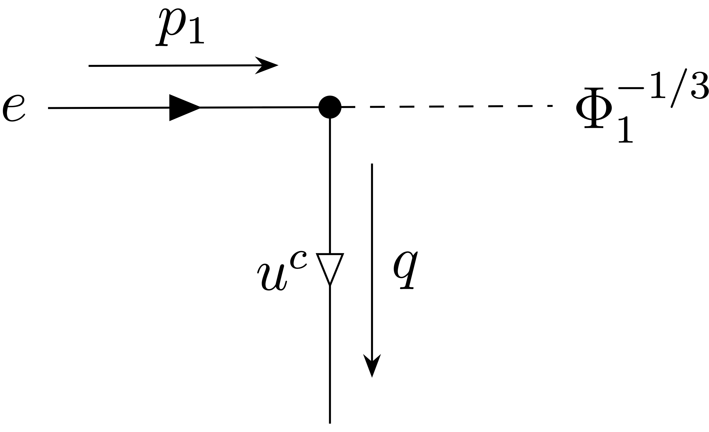
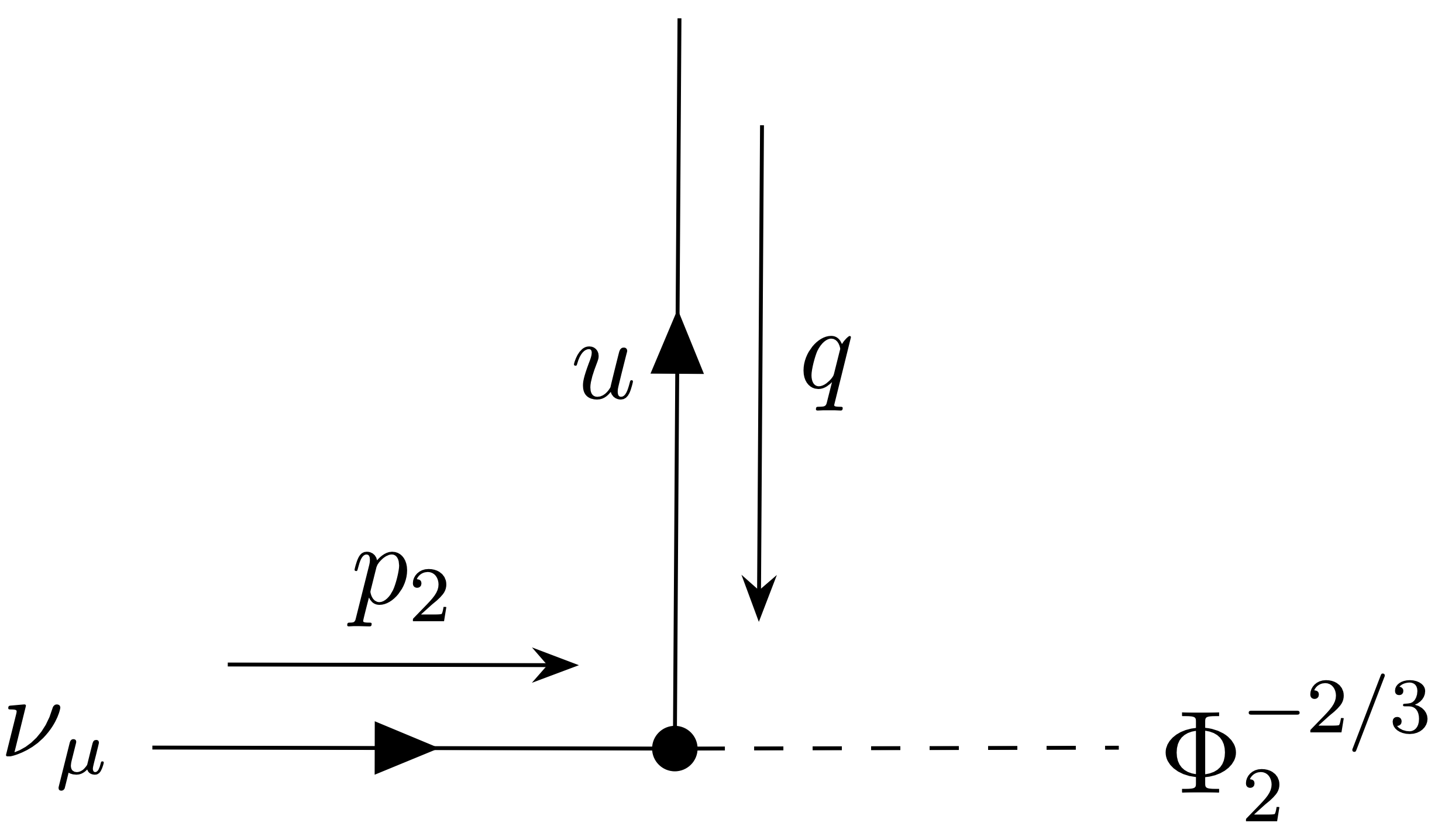
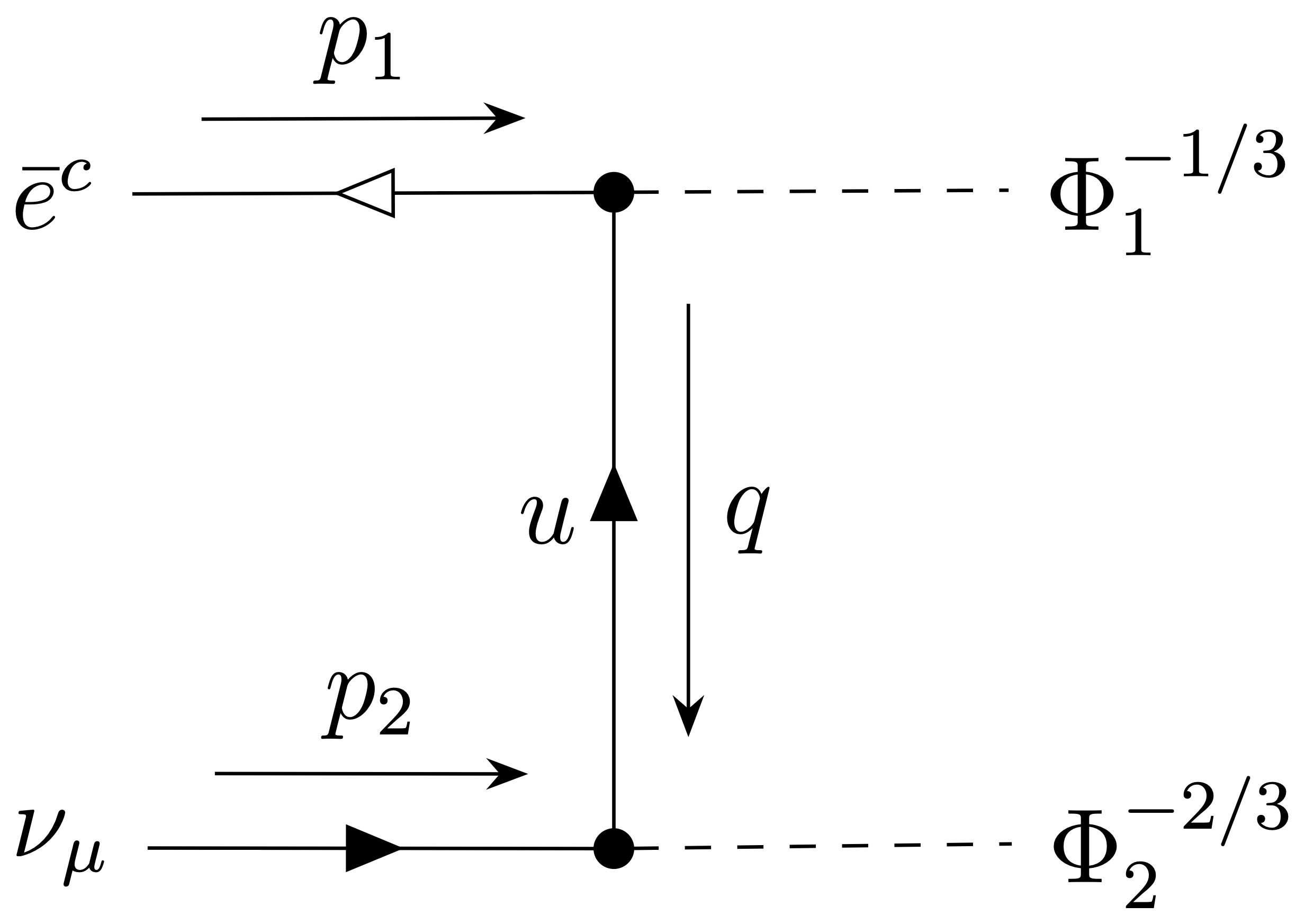
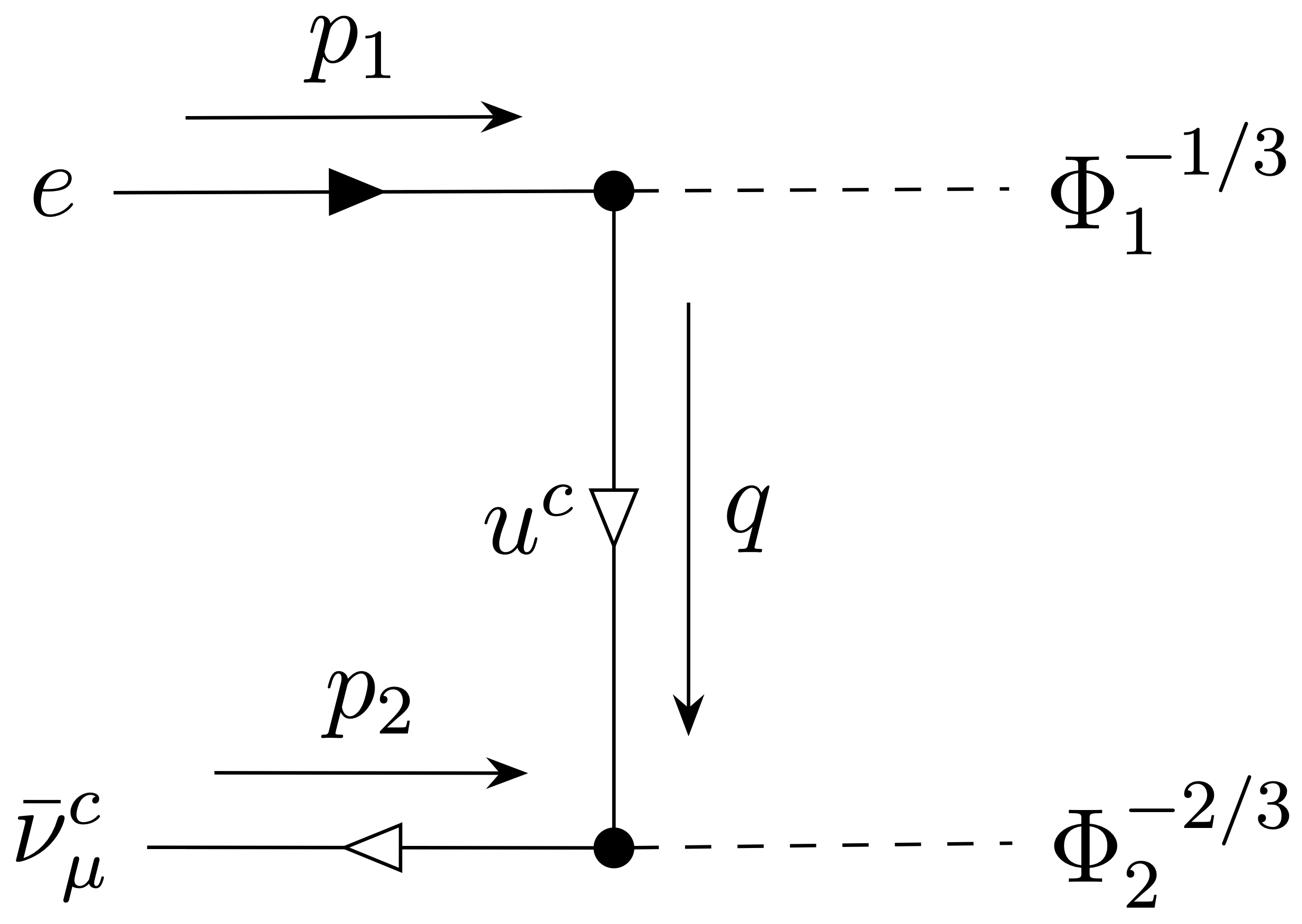
The Feynman diagram is shown in Fig. 1. Fig. 1(a) shows two parts of the diagram with clashing fermion line arrows for the up quark. In order to combine the two parts, the fermion arrows of one of them have to be inverted. In Fig. 1(b), the arrows of the upper part are inverted, in Fig. 1(c) the ones of the lower part. In the following, we will derive the analytic expressions for both of them, showing their equivalence. Choosing the reference order $(1,2)$ for the external states, the Feynman amplitude for the diagram in Fig. 1(b) reads

	$\displaystyle i\mathcal{M}$	$\displaystyle=\bar{v}^{(s_{1})}(\vec{p}_{1})\left(+iY_{1,11}^{LL}\text{P}_{\text{L}}+iY_{1,11}^{RR}\text{P}_{\text{R}}\right)\frac{-i\not{q}}{q^{2}+i\epsilon}\left(-iY_{2,12}^{RL}\text{P}_{\text{L}}\right)u^{(s_{2})}(\vec{p}_{2})$		(55)
		$\displaystyle=-i\frac{Y_{1,11}^{RR}Y_{2,12}^{RL}}{q^{2}+i\epsilon}\bar{v}^{(s_{1})}(\vec{p}_{1})\ \not{q}\text{P}_{\text{L}}\ u^{(s_{2})}(\vec{p}_{2})\,.$		(55)

The amplitude for the diagram in Fig. 1(c) is

	$\displaystyle i\mathcal{M}^{\prime}$	$\displaystyle=(-1)\bar{v}^{(s_{2})}(\vec{p}_{2})\left(-iY_{2,12}^{RL}\text{P}_{\text{L}}\right)\frac{i\not{q}}{q^{2}+i\epsilon}\left(+iY_{1,11}^{LL}\text{P}_{\text{L}}+iY_{1,11}^{RR}\text{P}_{\text{R}}\right)u^{(s_{1})}(\vec{p}_{1})$		(56)
		$\displaystyle=-i\frac{Y_{1,11}^{RR}Y_{2,12}^{RL}}{q^{2}+i\epsilon}\bar{v}^{(s_{2})}(\vec{p}_{2})\ \not{q}\text{P}_{\text{R}}\ u^{(s_{1})}(\vec{p}_{1})\,,$		(56)

where the factor $(-1)$ is added since the order of the external states is now reversed. The two amplitudes are equivalent, since

$\displaystyle i\mathcal{M}$	$\displaystyle\propto\bar{v}^{(s_{1})}(\vec{p}_{1})\ \not{q}\text{P}_{\text{L}}\ u^{(s_{2})}(\vec{p}_{2})=q_{\mu}\bar{v}^{(s_{1})}(\vec{p}_{1})\ \frac{\gamma^{\mu}-\gamma^{\mu}\gamma^{5}}{2}\ u^{(s_{2})}(\vec{p}_{2})$	(57)
	$\displaystyle=q_{\mu}u^{(s_{2})}(\vec{p}_{2})^{\intercal}\ \frac{\gamma^{\mu\intercal}-\left(\gamma^{\mu}\gamma^{5}\right)^{\intercal}}{2}\ \bar{v}^{(s_{1})}(\vec{p}_{1})^{\intercal}$
	$\displaystyle=q_{\mu}u^{(s_{2})}(\vec{p}_{2})^{\intercal}\ C^{-1}\frac{-\gamma^{\mu}-\gamma^{\mu}\gamma^{5}}{2}C\ \bar{v}^{(s_{1})}(\vec{p}_{1})^{\intercal}$
	$\displaystyle=q_{\mu}\bar{v}^{(s_{2})}(\vec{p}_{2})\ \frac{\gamma^{\mu}+\gamma^{\mu}\gamma^{5}}{2}\ u^{(s_{1})}(\vec{p}_{1})=\bar{v}^{(s_{2})}(\vec{p}_{2})\ \not{q}\text{P}_{\text{R}}\ u^{(s_{1})}(\vec{p}_{1})\propto i\mathcal{M}^{\prime}\,,$

where we have used Eq. (52) and

	$\displaystyle u^{(s)}(\vec{p})$	$\displaystyle=C\bar{v}^{(s)}(\vec{p})^{\intercal}\,,$		(58)
	$\displaystyle v^{(s)}(\vec{p})$	$\displaystyle=C\bar{u}^{(s)}(\vec{p})^{\intercal}$		(58)

for spinors $u,v$ , which can be derived from Eq. (44). This equivalence is true for all Feynman diagrams involving charge-conjugate fermions, as argued in Ref. [181].

A.2 Charge-Conjugate SM Fermion Feynman Rules

External Fields

The Feynman rules for the external charge-conjugate fermions are listed in this section. See Ref. [181] for details.

External Fermions
Diagram	Feynman Rule
	$u^{(s)}(\vec{p})$
	$\bar{u}^{(s)}(\vec{p})$
	$\bar{v}^{(s)}(\vec{p})$
	$v^{(s)}(\vec{p})$

Propagators

The propagators for the charge-conjugate SM fermions are given below. The fermion masses $m_{\ell_{i}},m_{u_{i}},m_{d_{i}}$ are defined in Eq. (18).

Interactions with SM Gauge Bosons

The Feynman rules for charge-conjugate SM fermion fields interacting with SM gauge fields are given below.

Interactions with the Higgs Field

The Feynman rules for charge-conjugate SM fermion fields interacting with Higgs field are given below.

Interactions with the Goldstone Bosons

The Feynman rules for charge-conjugate SM fermion fields interacting with SM Goldstone bosons are given below.

Interactions with LQs

The Feynman rules for LQ interactions with the charge-conjugate SM fermions are given below.

Acknowledgements

We thank Dario Müller and Francesco Saturnino for useful discussions. The work of A.C. is supported by a Professorship Grant (PP00P2_176884) of the Swiss National Science Foundation. L.S. thanks the Restaurant Veranda Bern for the use of their meeting room during the Covid-19 outbreak. The work of L.S. is supported by the “Excellence Scholarship & Opportunity Programme” of the ETH Zürich Foundation.

References

[1] J. C. Pati, A. Salam, Lepton Number as the Fourth Color, Phys. Rev. D 10 (1974) 275–289, [Erratum: Phys.Rev.D 11, 703–703 (1975)]. doi:10.1103/PhysRevD.10.275.
[2] H. Georgi, S. L. Glashow, Unity of All Elementary Particle Forces, Phys. Rev. Lett. 32 (1974) 438–441. doi:10.1103/PhysRevLett.32.438.
[3] H. Georgi, H. R. Quinn, S. Weinberg, Hierarchy of Interactions in Unified Gauge Theories, Phys. Rev. Lett. 33 (1974) 451–454. doi:10.1103/PhysRevLett.33.451.
[4] H. Fritzsch, P. Minkowski, Unified Interactions of Leptons and Hadrons, Annals Phys. 93 (1975) 193–266. doi:10.1016/0003-4916(75)90211-0.
[5] W. Buchmuller, R. Ruckl, D. Wyler, Leptoquarks in Lepton - Quark Collisions, Phys. Lett. B 191 (1987) 442–448, [Erratum: Phys.Lett.B 448, 320–320 (1999)]. doi:10.1016/0370-2693(87)90637-X.
[6] J. P. Lees, et al., Evidence for an excess of $\bar{B}\to D^{(*)}\tau^{-}\bar{\nu}_{\tau}$ decays, Phys. Rev. Lett. 109 (2012) 101802. arXiv:1205.5442, doi:10.1103/PhysRevLett.109.101802.
[7] J. P. Lees, et al., Measurement of an Excess of $\bar{B}\to D^{(*)}\tau^{-}\bar{\nu}_{\tau}$ Decays and Implications for Charged Higgs Bosons, Phys. Rev. D 88 (7) (2013) 072012. arXiv:1303.0571, doi:10.1103/PhysRevD.88.072012.
[8] R. Aaij, et al., Measurement of the ratio of branching fractions $\mathcal{B}(\bar{B}^{0}\to D^{*+}\tau^{-}\bar{\nu}_{\tau})/\mathcal{B}(\bar{B}^{0}\to D^{*+}\mu^{-}\bar{\nu}_{\mu})$ , Phys. Rev. Lett. 115 (11) (2015) 111803, [Erratum: Phys.Rev.Lett. 115, 159901 (2015)]. arXiv:1506.08614, doi:10.1103/PhysRevLett.115.111803.
[9] R. Aaij, et al., Test of Lepton Flavor Universality by the measurement of the $B^{0}\to D^{*-}\tau^{+}\nu_{\tau}$ branching fraction using three-prong $\tau$ decays, Phys. Rev. D 97 (7) (2018) 072013. arXiv:1711.02505, doi:10.1103/PhysRevD.97.072013.
[10] R. Aaij, et al., Measurement of the ratio of the $B^{0}\to D^{*-}\tau^{+}\nu_{\tau}$ and $B^{0}\to D^{*-}\mu^{+}\nu_{\mu}$ branching fractions using three-prong $\tau$ -lepton decays, Phys. Rev. Lett. 120 (17) (2018) 171802. arXiv:1708.08856, doi:10.1103/PhysRevLett.120.171802.
[11] A. Abdesselam, et al., Measurement of $\mathcal{R}(D)$ and $\mathcal{R}(D^{\ast})$ with a semileptonic tagging method (4 2019). arXiv:1904.08794.
[12] V. Khachatryan, et al., Observation of the rare $B^{0}_{s}\to\mu^{+}\mu^{-}$ decay from the combined analysis of CMS and LHCb data, Nature 522 (2015) 68–72. arXiv:1411.4413, doi:10.1038/nature14474.
[13] R. Aaij, et al., Angular analysis of the $B^{0}\to K^{*0}\mu^{+}\mu^{-}$ decay using 3 fb^-1 of integrated luminosity, JHEP 02 (2016) 104. arXiv:1512.04442, doi:10.1007/JHEP02(2016)104.
[14] A. Abdesselam, et al., Angular analysis of $B^{0}\to K^{\ast}(892)^{0}\ell^{+}\ell^{-}$ , in: LHC Ski 2016: A First Discussion of 13 TeV Results, 2016. arXiv:1604.04042.
[15] R. Aaij, et al., Test of lepton universality with $B^{0}\rightarrow K^{*0}\ell^{+}\ell^{-}$ decays, JHEP 08 (2017) 055. arXiv:1705.05802, doi:10.1007/JHEP08(2017)055.
[16] R. Aaij, et al., Search for lepton-universality violation in $B^{+}\to K^{+}\ell^{+}\ell^{-}$ decays, Phys. Rev. Lett. 122 (19) (2019) 191801. arXiv:1903.09252, doi:10.1103/PhysRevLett.122.191801.
[17] R. Aaij, et al., Measurement of $CP$ -Averaged Observables in the $B^{0}\rightarrow K^{*0}\mu^{+}\mu^{-}$ Decay, Phys. Rev. Lett. 125 (1) (2020) 011802. arXiv:2003.04831, doi:10.1103/PhysRevLett.125.011802.
[18] R. Aaij, et al., Test of lepton universality in beauty-quark decays (3 2021). arXiv:2103.11769.
[19] G. W. Bennett, et al., Final Report of the Muon E821 Anomalous Magnetic Moment Measurement at BNL, Phys. Rev. D 73 (2006) 072003. arXiv:hep-ex/0602035, doi:10.1103/PhysRevD.73.072003.
[20] B. Abi, et al., Measurement of the Positive Muon Anomalous Magnetic Moment to 0.46 ppm, Phys. Rev. Lett. 126 (14) (2021) 141801. arXiv:2104.03281, doi:10.1103/PhysRevLett.126.141801.
[21] Y. Amhis, et al., Averages of $b$ -hadron, $c$ -hadron, and $\tau$ -lepton properties as of summer 2016, Eur. Phys. J. C 77 (12) (2017) 895. arXiv:1612.07233, doi:10.1140/epjc/s10052-017-5058-4.
[22] C. Murgui, A. Peñuelas, M. Jung, A. Pich, Global fit to $b\to c\tau\nu$ transitions, JHEP 09 (2019) 103. arXiv:1904.09311, doi:10.1007/JHEP09(2019)103.
[23] R.-X. Shi, L.-S. Geng, B. Grinstein, S. Jäger, J. Martin Camalich, Revisiting the new-physics interpretation of the $b\to c\tau\nu$ data, JHEP 12 (2019) 065. arXiv:1905.08498, doi:10.1007/JHEP12(2019)065.
[24] M. Blanke, A. Crivellin, T. Kitahara, M. Moscati, U. Nierste, I. Nišandžić, Addendum to “Impact of polarization observables and $B_{c}\to\tau\nu$ on new physics explanations of the $b\to c\tau\nu$ anomaly”[Addendum: Phys.Rev.D 100, 035035 (2019)] (5 2019). arXiv:1905.08253, doi:10.1103/PhysRevD.100.035035.
[25] S. Kumbhakar, A. K. Alok, D. Kumar, S. U. Sankar, A global fit to $b\rightarrow c\tau\bar{\nu}$ anomalies after Moriond 2019, PoS EPS-HEP2019 (2020) 272. arXiv:1909.02840, doi:10.22323/1.364.0272.
[26] B. Capdevila, A. Crivellin, S. Descotes-Genon, J. Matias, J. Virto, Patterns of New Physics in $b\to s\ell^{+}\ell^{-}$ transitions in the light of recent data, JHEP 01 (2018) 093. arXiv:1704.05340, doi:10.1007/JHEP01(2018)093.
[27] W. Altmannshofer, P. Stangl, D. M. Straub, Interpreting Hints for Lepton Flavor Universality Violation, Phys. Rev. D 96 (5) (2017) 055008. arXiv:1704.05435, doi:10.1103/PhysRevD.96.055008.
[28] M. Algueró, B. Capdevila, A. Crivellin, S. Descotes-Genon, P. Masjuan, J. Matias, M. Novoa Brunet, J. Virto, Emerging patterns of New Physics with and without Lepton Flavour Universal contributions, Eur. Phys. J. C 79 (8) (2019) 714, [Addendum: Eur.Phys.J.C 80, 511 (2020)]. arXiv:1903.09578, doi:10.1140/epjc/s10052-019-7216-3.
[29] A. K. Alok, A. Dighe, S. Gangal, D. Kumar, Continuing search for new physics in $b\to s\mu\mu$ decays: two operators at a time, JHEP 06 (2019) 089. arXiv:1903.09617, doi:10.1007/JHEP06(2019)089.
[30] M. Ciuchini, A. M. Coutinho, M. Fedele, E. Franco, A. Paul, L. Silvestrini, M. Valli, New Physics in $b\to s\ell^{+}\ell^{-}$ confronts new data on Lepton Universality, Eur. Phys. J. C 79 (8) (2019) 719. arXiv:1903.09632, doi:10.1140/epjc/s10052-019-7210-9.
[31] J. Aebischer, W. Altmannshofer, D. Guadagnoli, M. Reboud, P. Stangl, D. M. Straub, $B$ -decay discrepancies after Moriond 2019, Eur. Phys. J. C 80 (3) (2020) 252. arXiv:1903.10434, doi:10.1140/epjc/s10052-020-7817-x.
[32] A. Arbey, T. Hurth, F. Mahmoudi, D. M. Santos, S. Neshatpour, Update on the $b\to s$ anomalies, Phys. Rev. D 100 (1) (2019) 015045. arXiv:1904.08399, doi:10.1103/PhysRevD.100.015045.
[33] D. Kumar, K. Kowalska, E. M. Sessolo, Global Bayesian Analysis of new physics in $b\to s\mu\mu$ transitions after Moriond-2019, in: 17th Conference on Flavor Physics and CP Violation, 2019. arXiv:1906.08596.
[34] T. Aoyama, et al., The anomalous magnetic moment of the muon in the Standard Model, Phys. Rept. 887 (2020) 1–166. arXiv:2006.04822, doi:10.1016/j.physrep.2020.07.006.
[35] C. Bobeth, D. van Dyk, M. Bordone, M. Jung, N. Gubernari, Lepton-flavour non-universality of $\bar{B}\to D^{*}\ell\bar{\nu}$ angular distributions in and beyond the Standard Model (4 2021). arXiv:2104.02094.
[36] R. Alonso, B. Grinstein, J. Martin Camalich, Lepton universality violation and lepton flavor conservation in $B$ -meson decays, JHEP 10 (2015) 184. arXiv:1505.05164, doi:10.1007/JHEP10(2015)184.
[37] L. Calibbi, A. Crivellin, T. Ota, Effective Field Theory Approach to $b\to s\ell\ell^{(^{\prime})}$ , $B\to K^{(*)}\nu\overline{\nu}$ and $B\to D^{(*)}\tau\nu$ with Third Generation Couplings, Phys. Rev. Lett. 115 (2015) 181801. arXiv:1506.02661, doi:10.1103/PhysRevLett.115.181801.
[38] G. Hiller, D. Loose, K. Schönwald, Leptoquark Flavor Patterns \& B Decay Anomalies, JHEP 12 (2016) 027. arXiv:1609.08895, doi:10.1007/JHEP12(2016)027.
[39] B. Bhattacharya, A. Datta, J.-P. Guévin, D. London, R. Watanabe, Simultaneous Explanation of the $R_{K}$ and $R_{D^{(*)}}$ Puzzles: a Model Analysis, JHEP 01 (2017) 015. arXiv:1609.09078, doi:10.1007/JHEP01(2017)015.
[40] D. Buttazzo, A. Greljo, G. Isidori, D. Marzocca, B-physics anomalies: a guide to combined explanations, JHEP 11 (2017) 044. arXiv:1706.07808, doi:10.1007/JHEP11(2017)044.
[41] R. Barbieri, G. Isidori, A. Pattori, F. Senia, Anomalies in $B$ -decays and $U(2)$ flavour symmetry, Eur. Phys. J. C 76 (2) (2016) 67. arXiv:1512.01560, doi:10.1140/epjc/s10052-016-3905-3.
[42] R. Barbieri, C. W. Murphy, F. Senia, B-decay Anomalies in a Composite Leptoquark Model, Eur. Phys. J. C 77 (1) (2017) 8. arXiv:1611.04930, doi:10.1140/epjc/s10052-016-4578-7.
[43] L. Calibbi, A. Crivellin, T. Li, Model of vector leptoquarks in view of the $B$ -physics anomalies, Phys. Rev. D 98 (11) (2018) 115002. arXiv:1709.00692, doi:10.1103/PhysRevD.98.115002.
[44] A. Crivellin, D. Müller, A. Signer, Y. Ulrich, Correlating lepton flavor universality violation in $B$ decays with $\mu\to e\gamma$ using leptoquarks, Phys. Rev. D 97 (1) (2018) 015019. arXiv:1706.08511, doi:10.1103/PhysRevD.97.015019.
[45] M. Bordone, C. Cornella, J. Fuentes-Martín, G. Isidori, Low-energy signatures of the $\mathrm{PS}^{3}$ model: from $B$ -physics anomalies to LFV, JHEP 10 (2018) 148. arXiv:1805.09328, doi:10.1007/JHEP10(2018)148.
[46] J. Kumar, D. London, R. Watanabe, Combined Explanations of the $b\to s\mu^{+}\mu^{-}$ and $b\to c\tau^{-}{\bar{\nu}}$ Anomalies: a General Model Analysis, Phys. Rev. D 99 (1) (2019) 015007. arXiv:1806.07403, doi:10.1103/PhysRevD.99.015007.
[47] A. Crivellin, C. Greub, D. Müller, F. Saturnino, Importance of Loop Effects in Explaining the Accumulated Evidence for New Physics in B Decays with a Vector Leptoquark, Phys. Rev. Lett. 122 (1) (2019) 011805. arXiv:1807.02068, doi:10.1103/PhysRevLett.122.011805.
[48] A. Crivellin, F. Saturnino, Explaining the Flavor Anomalies with a Vector Leptoquark (Moriond 2019 update), PoS DIS2019 (2019) 163. arXiv:1906.01222, doi:10.22323/1.352.0163.
[49] C. Cornella, J. Fuentes-Martin, G. Isidori, Revisiting the vector leptoquark explanation of the B-physics anomalies, JHEP 07 (2019) 168. arXiv:1903.11517, doi:10.1007/JHEP07(2019)168.
[50] M. Bordone, O. Catà, T. Feldmann, Effective Theory Approach to New Physics with Flavour: General Framework and a Leptoquark Example, JHEP 01 (2020) 067. arXiv:1910.02641, doi:10.1007/JHEP01(2020)067.
[51] J. Bernigaud, I. de Medeiros Varzielas, J. Talbert, Finite Family Groups for Fermionic and Leptoquark Mixing Patterns, JHEP 01 (2020) 194. arXiv:1906.11270, doi:10.1007/JHEP01(2020)194.
[52] J. Aebischer, A. Crivellin, C. Greub, QCD improved matching for semileptonic B decays with leptoquarks, Phys. Rev. D 99 (5) (2019) 055002. arXiv:1811.08907, doi:10.1103/PhysRevD.99.055002.
[53] J. Fuentes-Martín, G. Isidori, M. König, N. Selimović, Vector Leptoquarks Beyond Tree Level, Phys. Rev. D 101 (3) (2020) 035024. arXiv:1910.13474, doi:10.1103/PhysRevD.101.035024.
[54] O. Popov, M. A. Schmidt, G. White, $R_{2}$ as a single leptoquark solution to $R_{D^{(*)}}$ and $R_{K^{(*)}}$ , Phys. Rev. D 100 (3) (2019) 035028. arXiv:1905.06339, doi:10.1103/PhysRevD.100.035028.
[55] S. Fajfer, N. Košnik, Vector leptoquark resolution of $R_{K}$ and $R_{D^{(*)}}$ puzzles, Phys. Lett. B 755 (2016) 270–274. arXiv:1511.06024, doi:10.1016/j.physletb.2016.02.018.
[56] M. Blanke, A. Crivellin, $B$ Meson Anomalies in a Pati-Salam Model within the Randall-Sundrum Background, Phys. Rev. Lett. 121 (1) (2018) 011801. arXiv:1801.07256, doi:10.1103/PhysRevLett.121.011801.
[57] I. de Medeiros Varzielas, J. Talbert, Simplified Models of Flavourful Leptoquarks, Eur. Phys. J. C 79 (6) (2019) 536. arXiv:1901.10484, doi:10.1140/epjc/s10052-019-7047-2.
[58] I. de Medeiros Varzielas, G. Hiller, Clues for flavor from rare lepton and quark decays, JHEP 06 (2015) 072. arXiv:1503.01084, doi:10.1007/JHEP06(2015)072.
[59] A. Crivellin, D. Müller, F. Saturnino, Flavor Phenomenology of the Leptoquark Singlet-Triplet Model, JHEP 06 (2020) 020. arXiv:1912.04224, doi:10.1007/JHEP06(2020)020.
[60] S. Saad, Combined explanations of $(g-2)_{\mu}$ , $R_{D^{(*)}}$ , $R_{K^{(*)}}$ anomalies in a two-loop radiative neutrino mass model, Phys. Rev. D 102 (1) (2020) 015019. arXiv:2005.04352, doi:10.1103/PhysRevD.102.015019.
[61] S. Saad, A. Thapa, Common origin of neutrino masses and $R_{D^{(\ast)}}$ , $R_{K^{(\ast)}}$ anomalies, Phys. Rev. D 102 (1) (2020) 015014. arXiv:2004.07880, doi:10.1103/PhysRevD.102.015014.
[62] V. Gherardi, D. Marzocca, E. Venturini, Low-energy phenomenology of scalar leptoquarks at one-loop accuracy, JHEP 01 (2021) 138. arXiv:2008.09548, doi:10.1007/JHEP01(2021)138.
[63] L. Da Rold, F. Lamagna, A model for the Singlet-Triplet Leptoquarks (11 2020). arXiv:2011.10061.
[64] M. Bordone, C. Cornella, J. Fuentes-Martin, G. Isidori, A three-site gauge model for flavor hierarchies and flavor anomalies, Phys. Lett. B 779 (2018) 317–323. arXiv:1712.01368, doi:10.1016/j.physletb.2018.02.011.
[65] A. Biswas, D. Kumar Ghosh, N. Ghosh, A. Shaw, A. K. Swain, Collider signature of $U_{1}$ Leptoquark and constraints from $b\to c$ observables, J. Phys. G 47 (4) (2020) 045005. arXiv:1808.04169, doi:10.1088/1361-6471/ab6948.
[66] J. Heeck, D. Teresi, Pati-Salam explanations of the B-meson anomalies, JHEP 12 (2018) 103. arXiv:1808.07492, doi:10.1007/JHEP12(2018)103.
[67] S. Sahoo, R. Mohanta, Scalar leptoquarks and the rare $B$ meson decays, Phys. Rev. D 91 (9) (2015) 094019. arXiv:1501.05193, doi:10.1103/PhysRevD.91.094019.
[68] C.-H. Chen, T. Nomura, H. Okada, Explanation of $B\to K^{(*)}\ell^{+}\ell^{-}$ and muon $g-2$ , and implications at the LHC, Phys. Rev. D 94 (11) (2016) 115005. arXiv:1607.04857, doi:10.1103/PhysRevD.94.115005.
[69] U. K. Dey, D. Kar, M. Mitra, M. Spannowsky, A. C. Vincent, Searching for Leptoquarks at IceCube and the LHC, Phys. Rev. D 98 (3) (2018) 035014. arXiv:1709.02009, doi:10.1103/PhysRevD.98.035014.
[70] D. Bečirević, O. Sumensari, A leptoquark model to accommodate $R_{K}^{\mathrm{exp}}<R_{K}^{\mathrm{SM}}$ and $R_{K^{\ast}}^{\mathrm{exp}}<R_{K^{\ast}}^{\mathrm{SM}}$ , JHEP 08 (2017) 104. arXiv:1704.05835, doi:10.1007/JHEP08(2017)104.
[71] B. Chauhan, B. Kindra, A. Narang, Discrepancies in simultaneous explanation of flavor anomalies and IceCube PeV events using leptoquarks, Phys. Rev. D 97 (9) (2018) 095007. arXiv:1706.04598, doi:10.1103/PhysRevD.97.095007.
[72] D. Bečirević, I. Doršner, S. Fajfer, N. Košnik, D. A. Faroughy, O. Sumensari, Scalar leptoquarks from grand unified theories to accommodate the $B$ -physics anomalies, Phys. Rev. D 98 (5) (2018) 055003. arXiv:1806.05689, doi:10.1103/PhysRevD.98.055003.
[73] S. Fajfer, J. F. Kamenik, I. Nisandzic, J. Zupan, Implications of Lepton Flavor Universality Violations in B Decays, Phys. Rev. Lett. 109 (2012) 161801. arXiv:1206.1872, doi:10.1103/PhysRevLett.109.161801.
[74] N. G. Deshpande, A. Menon, Hints of R-parity violation in B decays into $\tau\nu$ , JHEP 01 (2013) 025. arXiv:1208.4134, doi:10.1007/JHEP01(2013)025.
[75] M. Freytsis, Z. Ligeti, J. T. Ruderman, Flavor models for $\bar{B}\to D^{(*)}\tau\bar{\nu}$ , Phys. Rev. D 92 (5) (2015) 054018. arXiv:1506.08896, doi:10.1103/PhysRevD.92.054018.
[76] M. Bauer, M. Neubert, Minimal Leptoquark Explanation for the R ${}_{D^{(*)}}$ , R_K , and $(g-2)_{g}$ Anomalies, Phys. Rev. Lett. 116 (14) (2016) 141802. arXiv:1511.01900, doi:10.1103/PhysRevLett.116.141802.
[77] X.-Q. Li, Y.-D. Yang, X. Zhang, Revisiting the one leptoquark solution to the R(D^(∗)) anomalies and its phenomenological implications, JHEP 08 (2016) 054. arXiv:1605.09308, doi:10.1007/JHEP08(2016)054.
[78] J. Zhu, H.-M. Gan, R.-M. Wang, Y.-Y. Fan, Q. Chang, Y.-G. Xu, Probing the R-parity violating supersymmetric effects in the exclusive $b\to c\ell^{-}\bar{\nu}_{\ell}$ decays, Phys. Rev. D 93 (9) (2016) 094023. arXiv:1602.06491, doi:10.1103/PhysRevD.93.094023.
[79] O. Popov, G. A. White, One Leptoquark to unify them? Neutrino masses and unification in the light of $(g-2)_{\mu}$ , $R_{D^{(\star)}}$ and $R_{K}$ anomalies, Nucl. Phys. B 923 (2017) 324–338. arXiv:1611.04566, doi:10.1016/j.nuclphysb.2017.08.007.
[80] N. G. Deshpande, X.-G. He, Consequences of R-parity violating interactions for anomalies in $\bar{B}\to D^{(*)}\tau\bar{\nu}$ and $b\to s\mu^{+}\mu^{-}$ , Eur. Phys. J. C 77 (2) (2017) 134. arXiv:1608.04817, doi:10.1140/epjc/s10052-017-4707-y.
[81] D. Bečirević, N. Košnik, O. Sumensari, R. Zukanovich Funchal, Palatable Leptoquark Scenarios for Lepton Flavor Violation in Exclusive $b\to s\ell_{1}\ell_{2}$ modes, JHEP 11 (2016) 035. arXiv:1608.07583, doi:10.1007/JHEP11(2016)035.
[82] Y. Cai, J. Gargalionis, M. A. Schmidt, R. R. Volkas, Reconsidering the One Leptoquark solution: flavor anomalies and neutrino mass, JHEP 10 (2017) 047. arXiv:1704.05849, doi:10.1007/JHEP10(2017)047.
[83] W. Altmannshofer, P. S. Bhupal Dev, A. Soni, $R_{D^{(*)}}$ anomaly: A possible hint for natural supersymmetry with $R$ -parity violation, Phys. Rev. D 96 (9) (2017) 095010. arXiv:1704.06659, doi:10.1103/PhysRevD.96.095010.
[84] S. Kamali, A. Rashed, A. Datta, New physics in inclusive $B\to X_{c}\ell\bar{\nu}$ decay in light of $R(D^{(*)})$ measurements, Phys. Rev. D 97 (9) (2018) 095034. arXiv:1801.08259, doi:10.1103/PhysRevD.97.095034.
[85] T. Mandal, S. Mitra, S. Raz, $R_{D^{(*)}}$ motivated $\mathcal{S}_{1}$ leptoquark scenarios: Impact of interference on the exclusion limits from LHC data, Phys. Rev. D 99 (5) (2019) 055028. arXiv:1811.03561, doi:10.1103/PhysRevD.99.055028.
[86] A. Azatov, D. Bardhan, D. Ghosh, F. Sgarlata, E. Venturini, Anatomy of $b\to c\tau\nu$ anomalies, JHEP 11 (2018) 187. arXiv:1805.03209, doi:10.1007/JHEP11(2018)187.
[87] J. Zhu, B. Wei, J.-H. Sheng, R.-M. Wang, Y. Gao, G.-R. Lu, Probing the R-parity violating supersymmetric effects in $B_{c}\to J/\psi\ell^{-}\bar{\nu}_{\ell},\eta_{c}\ell^{-}\bar{\nu}_{\ell}$ and $\Lambda_{b}\to\Lambda_{c}\ell^{-}\bar{\nu}_{\ell}$ decays, Nucl. Phys. B 934 (2018) 380–395. arXiv:1801.00917, doi:10.1016/j.nuclphysb.2018.07.011.
[88] A. Angelescu, D. Bečirević, D. A. Faroughy, O. Sumensari, Closing the window on single leptoquark solutions to the $B$ -physics anomalies, JHEP 10 (2018) 183. arXiv:1808.08179, doi:10.1007/JHEP10(2018)183.
[89] T. J. Kim, P. Ko, J. Li, J. Park, P. Wu, Correlation between ${R}_{D^{\left(\ast\right)}}$ and top quark FCNC decays in leptoquark models, JHEP 07 (2019) 025. arXiv:1812.08484, doi:10.1007/JHEP07(2019)025.
[90] U. Aydemir, T. Mandal, S. Mitra, Addressing the ${\mathbf{R}_{D^{(*)}}}$ anomalies with an ${\mathbf{S}_{1}}$ leptoquark from $\mathbf{SO(10)}$ grand unification, Phys. Rev. D 101 (1) (2020) 015011. arXiv:1902.08108, doi:10.1103/PhysRevD.101.015011.
[91] A. Crivellin, F. Saturnino, Correlating tauonic $B$ decays with the neutron electric dipole moment via a scalar leptoquark, Phys. Rev. D 100 (11) (2019) 115014. arXiv:1905.08257, doi:10.1103/PhysRevD.100.115014.
[92] H. Yan, Y.-D. Yang, X.-B. Yuan, Phenomenology of $b\to c\tau\bar{\nu}$ decays in a scalar leptoquark model, Chin. Phys. C 43 (8) (2019) 083105. arXiv:1905.01795, doi:10.1088/1674-1137/43/8/083105.
[93] A. Crivellin, D. Müller, T. Ota, Simultaneous explanation of R(D^(∗)) and $b\to s\mu^{+}\mu^{-}$ : the last scalar leptoquarks standing, JHEP 09 (2017) 040. arXiv:1703.09226, doi:10.1007/JHEP09(2017)040.
[94] D. Marzocca, Addressing the B-physics anomalies in a fundamental Composite Higgs Model, JHEP 07 (2018) 121. arXiv:1803.10972, doi:10.1007/JHEP07(2018)121.
[95] I. Bigaran, J. Gargalionis, R. R. Volkas, A near-minimal leptoquark model for reconciling flavour anomalies and generating radiative neutrino masses, JHEP 10 (2019) 106. arXiv:1906.01870, doi:10.1007/JHEP10(2019)106.
[96] P. S. Bhupal Dev, R. Mohanta, S. Patra, S. Sahoo, Unified explanation of flavor anomalies, radiative neutrino masses, and ANITA anomalous events in a vector leptoquark model, Phys. Rev. D 102 (9) (2020) 095012. arXiv:2004.09464, doi:10.1103/PhysRevD.102.095012.
[97] W. Altmannshofer, P. S. B. Dev, A. Soni, Y. Sui, Addressing R ${}_{D^{(*)}}$ , R ${}_{K^{(*)}}$ , muon $g-2$ and ANITA anomalies in a minimal $R$ -parity violating supersymmetric framework, Phys. Rev. D 102 (1) (2020) 015031. arXiv:2002.12910, doi:10.1103/PhysRevD.102.015031.
[98] J. Fuentes-Martín, P. Stangl, Third-family quark-lepton unification with a fundamental composite Higgs, Phys. Lett. B 811 (2020) 135953. arXiv:2004.11376, doi:10.1016/j.physletb.2020.135953.
[99] A. Djouadi, T. Kohler, M. Spira, J. Tutas, (e b), (e t) TYPE LEPTOQUARKS AT e p COLLIDERS, Z. Phys. C 46 (1990) 679–686. doi:10.1007/BF01560270.
[100] D. Chakraverty, D. Choudhury, A. Datta, A Nonsupersymmetric resolution of the anomalous muon magnetic moment, Phys. Lett. B 506 (2001) 103–108. arXiv:hep-ph/0102180, doi:10.1016/S0370-2693(01)00419-1.
[101] K.-m. Cheung, Muon anomalous magnetic moment and leptoquark solutions, Phys. Rev. D 64 (2001) 033001. arXiv:hep-ph/0102238, doi:10.1103/PhysRevD.64.033001.
[102] C. Biggio, M. Bordone, L. Di Luzio, G. Ridolfi, Massive vectors and loop observables: the $g-2$ case, JHEP 10 (2016) 002. arXiv:1607.07621, doi:10.1007/JHEP10(2016)002.
[103] S. Davidson, D. C. Bailey, B. A. Campbell, Model independent constraints on leptoquarks from rare processes, Z. Phys. C 61 (1994) 613–644. arXiv:hep-ph/9309310, doi:10.1007/BF01552629.
[104] G. Couture, H. Konig, Bounds on second generation scalar leptoquarks from the anomalous magnetic moment of the muon, Phys. Rev. D 53 (1996) 555–557. arXiv:hep-ph/9507263, doi:10.1103/PhysRevD.53.555.
[105] U. Mahanta, Implications of BNL measurement of delta a(mu) on a class of scalar leptoquark interactions, Eur. Phys. J. C 21 (2001) 171–173. arXiv:hep-ph/0102176, doi:10.1007/s100520100705.
[106] F. S. Queiroz, K. Sinha, A. Strumia, Leptoquarks, Dark Matter, and Anomalous LHC Events, Phys. Rev. D 91 (3) (2015) 035006. arXiv:1409.6301, doi:10.1103/PhysRevD.91.035006.
[107] E. Coluccio Leskow, G. D’Ambrosio, A. Crivellin, D. Müller, $(g-2)\mu$ , lepton flavor violation, and $Z$ decays with leptoquarks: Correlations and future prospects, Phys. Rev. D 95 (5) (2017) 055018. arXiv:1612.06858, doi:10.1103/PhysRevD.95.055018.
[108] C.-H. Chen, T. Nomura, H. Okada, Excesses of muon $g-2$ , $R_{D^{(\ast)}}$ , and $R_{K}$ in a leptoquark model, Phys. Lett. B 774 (2017) 456–464. arXiv:1703.03251, doi:10.1016/j.physletb.2017.10.005.
[109] D. Das, C. Hati, G. Kumar, N. Mahajan, Towards a unified explanation of $R_{D^{(\ast)}}$ , $R_{K}$ and $(g-2)_{\mu}$ anomalies in a left-right model with leptoquarks, Phys. Rev. D 94 (2016) 055034. arXiv:1605.06313, doi:10.1103/PhysRevD.94.055034.
[110] A. Crivellin, M. Hoferichter, P. Schmidt-Wellenburg, Combined explanations of $(g-2)_{\mu,e}$ and implications for a large muon EDM, Phys. Rev. D 98 (11) (2018) 113002. arXiv:1807.11484, doi:10.1103/PhysRevD.98.113002.
[111] K. Kowalska, E. M. Sessolo, Y. Yamamoto, Constraints on charmphilic solutions to the muon g-2 with leptoquarks, Phys. Rev. D 99 (5) (2019) 055007. arXiv:1812.06851, doi:10.1103/PhysRevD.99.055007.
[112] I. Doršner, S. Fajfer, O. Sumensari, Muon $g-2$ and scalar leptoquark mixing, JHEP 06 (2020) 089. arXiv:1910.03877, doi:10.1007/JHEP06(2020)089.
[113] L. Delle Rose, C. Marzo, L. Marzola, Simplified leptoquark models for precision $l_{i}\rightarrow l_{f}\gamma$ experiments: two-loop structure of $O(\alpha_{S}Y^{2})$ corrections, Phys. Rev. D 102 (11) (2020) 115020. arXiv:2005.12389, doi:10.1103/PhysRevD.102.115020.
[114] I. Bigaran, R. R. Volkas, Getting chirality right: Single scalar leptoquark solutions to the $(g-2)_{e,\mu}$ puzzle, Phys. Rev. D 102 (7) (2020) 075037. arXiv:2002.12544, doi:10.1103/PhysRevD.102.075037.
[115] I. Doršner, S. Fajfer, S. Saad, $\mu\to e\gamma$ selecting scalar leptoquark solutions for the $(g-2)_{e,\mu}$ puzzles, Phys. Rev. D 102 (7) (2020) 075007. arXiv:2006.11624, doi:10.1103/PhysRevD.102.075007.
[116] K. S. Babu, P. S. B. Dev, S. Jana, A. Thapa, Unified framework for $B$ -anomalies, muon $g-2$ and neutrino masses, JHEP 03 (2021) 179. arXiv:2009.01771, doi:10.1007/JHEP03(2021)179.
[117] A. Crivellin, D. Mueller, F. Saturnino, Correlating $h\to\mu^{+}\mu^{-}$ to the Anomalous Magnetic Moment of the Muon via Leptoquarks (8 2020). arXiv:2008.02643.
[118] A. Carvunis, A. Crivellin, D. Guadagnoli, S. Gangal, The Forward-Backward Asymmetry in $B\to D^{*}\ell\nu$ : One more hint for Scalar Leptoquarks? (6 2021). arXiv:2106.09610.
[119] M. Kramer, T. Plehn, M. Spira, P. M. Zerwas, Pair production of scalar leptoquarks at the Tevatron, Phys. Rev. Lett. 79 (1997) 341–344. arXiv:hep-ph/9704322, doi:10.1103/PhysRevLett.79.341.
[120] M. Kramer, T. Plehn, M. Spira, P. M. Zerwas, Pair production of scalar leptoquarks at the CERN LHC, Phys. Rev. D 71 (2005) 057503. arXiv:hep-ph/0411038, doi:10.1103/PhysRevD.71.057503.
[121] D. A. Faroughy, A. Greljo, J. F. Kamenik, Confronting lepton flavor universality violation in B decays with high- $p_{T}$ tau lepton searches at LHC, Phys. Lett. B 764 (2017) 126–134. arXiv:1609.07138, doi:10.1016/j.physletb.2016.11.011.
[122] A. Greljo, D. Marzocca, High- $p_{T}$ dilepton tails and flavor physics, Eur. Phys. J. C 77 (8) (2017) 548. arXiv:1704.09015, doi:10.1140/epjc/s10052-017-5119-8.
[123] J. Blumlein, E. Boos, A. Kryukov, Leptoquark pair production in hadronic interactions, Z. Phys. C 76 (1997) 137–153. arXiv:hep-ph/9610408, doi:10.1007/s002880050538.
[124] I. Doršner, S. Fajfer, D. A. Faroughy, N. Košnik, The role of the $S_{3}$ GUT leptoquark in flavor universality and collider searches, JHEP 10 (2017) 188. arXiv:1706.07779, doi:10.1007/JHEP10(2017)188.
[125] A. Cerri, et al., Report from Working Group 4: Opportunities in Flavour Physics at the HL-LHC and HE-LHC, CERN Yellow Rep. Monogr. 7 (2019) 867–1158. arXiv:1812.07638, doi:10.23731/CYRM-2019-007.867.
[126] P. Bandyopadhyay, R. Mandal, Revisiting scalar leptoquark at the LHC, Eur. Phys. J. C 78 (2018) 491. arXiv:1801.04253, doi:10.1140/epjc/s10052-018-5959-x.
[127] G. Hiller, D. Loose, I. Nišandžić, Flavorful leptoquarks at hadron colliders, Phys. Rev. D 97 (7) (2018) 075004. arXiv:1801.09399, doi:10.1103/PhysRevD.97.075004.
[128] T. Faber, M. Hudec, H. Kolešová, Y. Liu, M. Malinsky, W. Porod, F. Staub, Collider phenomenology of a unified leptoquark model, Phys. Rev. D 101 (9) (2020) 095024. arXiv:1812.07592, doi:10.1103/PhysRevD.101.095024.
[129] M. Schmaltz, Y.-M. Zhong, The leptoquark Hunter’s guide: large coupling, JHEP 01 (2019) 132. arXiv:1810.10017, doi:10.1007/JHEP01(2019)132.
[130] K. Chandak, T. Mandal, S. Mitra, Hunting for scalar leptoquarks with boosted tops and light leptons, Phys. Rev. D 100 (7) (2019) 075019. arXiv:1907.11194, doi:10.1103/PhysRevD.100.075019.
[131] B. C. Allanach, T. Corbett, M. Madigan, Sensitivity of Future Hadron Colliders to Leptoquark Pair Production in the Di-Muon Di-Jets Channel, Eur. Phys. J. C 80 (2) (2020) 170. arXiv:1911.04455, doi:10.1140/epjc/s10052-020-7722-3.
[132] L. Buonocore, U. Haisch, P. Nason, F. Tramontano, G. Zanderighi, Lepton-Quark Collisions at the Large Hadron Collider, Phys. Rev. Lett. 125 (23) (2020) 231804. arXiv:2005.06475, doi:10.1103/PhysRevLett.125.231804.
[133] U. Haisch, G. Polesello, Resonant third-generation leptoquark signatures at the Large Hadron Collider (12 2020). arXiv:2012.11474.
[134] C. Borschensky, B. Fuks, A. Kulesza, D. Schwartländer, Scalar leptoquark pair production at hadron colliders, Phys. Rev. D 101 (11) (2020) 115017. arXiv:2002.08971, doi:10.1103/PhysRevD.101.115017.
[135] A. Crivellin, L. Schnell, Addendum to: Combined Constraints on First Generation Leptoquarks (4 2021). arXiv:2104.06417.
[136] A. Crivellin, C. Greub, D. Müller, F. Saturnino, Scalar Leptoquarks in Leptonic Processes, JHEP 02 (2021) 182. arXiv:2010.06593, doi:10.1007/JHEP02(2021)182.
[137] E. Keith, E. Ma, S, T, and leptoquarks at HERA, Phys. Rev. Lett. 79 (1997) 4318–4320. arXiv:hep-ph/9707214, doi:10.1103/PhysRevLett.79.4318.
[138] I. Doršner, S. Fajfer, A. Greljo, J. F. Kamenik, N. Košnik, Physics of leptoquarks in precision experiments and at particle colliders, Phys. Rept. 641 (2016) 1–68. arXiv:1603.04993, doi:10.1016/j.physrep.2016.06.001.
[139] A. Bhaskar, D. Das, B. De, S. Mitra, Enhancing scalar productions with leptoquarks at the LHC, Phys. Rev. D 102 (3) (2020) 035002. arXiv:2002.12571, doi:10.1103/PhysRevD.102.035002.
[140] J. Zhang, C.-X. Yue, C.-H. Li, S. Yang, Constraints on scalar and vector leptoquarks from the LHC Higgs data (5 2019). arXiv:1905.04074.
[141] V. Gherardi, D. Marzocca, E. Venturini, Matching scalar leptoquarks to the SMEFT at one loop, JHEP 07 (2020) 225, [Erratum: JHEP 01, 006 (2021)]. arXiv:2003.12525, doi:10.1007/JHEP07(2020)225.
[142] A. Crivellin, D. Müller, F. Saturnino, Leptoquarks in oblique corrections and Higgs signal strength: status and prospects, JHEP 11 (2020) 094. arXiv:2006.10758, doi:10.1007/JHEP11(2020)094.
[143] O. U. Shanker, Flavor Violation, Scalar Particles and Leptoquarks, Nucl. Phys. B 206 (1982) 253–272. doi:10.1016/0550-3213(82)90534-X.
[144] O. U. Shanker, $\pi\ell$ 2, $K\ell$ 3 and $K^{0}-\bar{K}$ 0 Constraints on Leptoquarks and Supersymmetric Particles, Nucl. Phys. B 204 (1982) 375–386. doi:10.1016/0550-3213(82)90196-1.
[145] M. Leurer, A Comprehensive study of leptoquark bounds, Phys. Rev. D 49 (1994) 333–342. arXiv:hep-ph/9309266, doi:10.1103/PhysRevD.49.333.
[146] M. Leurer, Bounds on vector leptoquarks, Phys. Rev. D 50 (1994) 536–541. arXiv:hep-ph/9312341, doi:10.1103/PhysRevD.50.536.
[147] Y. Grossman, E. Passemar, S. Schacht, On the Statistical Treatment of the Cabibbo Angle Anomaly, JHEP 07 (2020) 068. arXiv:1911.07821, doi:10.1007/JHEP07(2020)068.
[148] C.-Y. Seng, X. Feng, M. Gorchtein, L.-C. Jin, Joint lattice QCD–dispersion theory analysis confirms the quark-mixing top-row unitarity deficit, Phys. Rev. D 101 (11) (2020) 111301. arXiv:2003.11264, doi:10.1103/PhysRevD.101.111301.
[149] B. Belfatto, R. Beradze, Z. Berezhiani, The CKM unitarity problem: A trace of new physics at the TeV scale?, Eur. Phys. J. C 80 (2) (2020) 149. arXiv:1906.02714, doi:10.1140/epjc/s10052-020-7691-6.
[150] A. M. Coutinho, A. Crivellin, C. A. Manzari, Global Fit to Modified Neutrino Couplings and the Cabibbo-Angle Anomaly, Phys. Rev. Lett. 125 (7) (2020) 071802. arXiv:1912.08823, doi:10.1103/PhysRevLett.125.071802.
[151] A. Crivellin, M. Hoferichter, $\beta$ Decays as Sensitive Probes of Lepton Flavor Universality, Phys. Rev. Lett. 125 (11) (2020) 111801. arXiv:2002.07184, doi:10.1103/PhysRevLett.125.111801.
[152] B. Capdevila, A. Crivellin, C. A. Manzari, M. Montull, Explaining $b\to s\ell^{+}\ell^{-}$ and the Cabibbo angle anomaly with a vector triplet, Phys. Rev. D 103 (1) (2021) 015032. arXiv:2005.13542, doi:10.1103/PhysRevD.103.015032.
[153] A. Crivellin, F. Kirk, C. A. Manzari, M. Montull, Global Electroweak Fit and Vector-Like Leptons in Light of the Cabibbo Angle Anomaly, JHEP 12 (2020) 166. arXiv:2008.01113, doi:10.1007/JHEP12(2020)166.
[154] M. Kirk, Cabibbo anomaly versus electroweak precision tests: An exploration of extensions of the Standard Model, Phys. Rev. D 103 (3) (2021) 035004. arXiv:2008.03261, doi:10.1103/PhysRevD.103.035004.
[155] A. K. Alok, A. Dighe, S. Gangal, J. Kumar, The role of non-universal $Z$ couplings in explaining the $V_{us}$ anomaly (10 2020). arXiv:2010.12009.
[156] A. Crivellin, C. A. Manzari, M. Alguero, J. Matias, Combined Explanation of the $Z\to b\bar{b}$ Forward-Backward Asymmetry, the Cabibbo Angle Anomaly, $\tau\to\mu\nu\nu$ and $b\to s\ell^{+}\ell^{-}$ Data (10 2020). arXiv:2010.14504.
[157] A. Crivellin, F. Kirk, C. A. Manzari, L. Panizzi, Searching for Lepton Flavour (Universality) Violation and Collider Signals from a Singly-Charged Scalar Singlet (12 2020). arXiv:2012.09845.
[158] A. Crivellin, M. Hoferichter, C. A. Manzari, The Fermi constant from muon decay versus electroweak fits and CKM unitarity (2 2021). arXiv:2102.02825.
[159] B. Belfatto, Z. Berezhiani, Are the CKM anomalies induced by vector-like quarks? Limits from flavor changing and Standard Model precision tests (3 2021). arXiv:2103.05549.
[160] G. C. Branco, J. T. Penedo, P. M. F. Pereira, M. N. Rebelo, J. I. Silva-Marcos, Addressing the CKM Unitarity Problem with a Vector-like Up Quark (3 2021). arXiv:2103.13409.
[161] C. Bobeth, A. J. Buras, Leptoquarks meet $\varepsilon^{\prime}/\varepsilon$ and rare Kaon processes, JHEP 02 (2018) 101. arXiv:1712.01295, doi:10.1007/JHEP02(2018)101.
[162] I. Doršner, S. Fajfer, M. Patra, A comparative study of the $S_{1}$ and $U_{1}$ leptoquark effects in the light quark regime, Eur. Phys. J. C 80 (3) (2020) 204. arXiv:1906.05660, doi:10.1140/epjc/s10052-020-7754-8.
[163] R. Mandal, A. Pich, Constraints on scalar leptoquarks from lepton and kaon physics, JHEP 12 (2019) 089. arXiv:1908.11155, doi:10.1007/JHEP12(2019)089.
[164] A. Greljo, P. Stangl, A. E. Thomsen, A Model of Muon Anomalies (3 2021). arXiv:2103.13991.
[165] J. Gargalionis, I. Popa-Mateiu, R. R. Volkas, Radiative neutrino mass model from a mass dimension-11 $\Delta L=2$ effective operator, JHEP 03 (2020) 150. arXiv:1912.12386, doi:10.1007/JHEP03(2020)150.
[166] A. Alloul, N. D. Christensen, C. Degrande, C. Duhr, B. Fuks, FeynRules 2.0 - A complete toolbox for tree-level phenomenology, Comput. Phys. Commun. 185 (2014) 2250–2300. arXiv:1310.1921, doi:10.1016/j.cpc.2014.04.012.
[167] T. Hahn, Generating Feynman diagrams and amplitudes with FeynArts 3, Comput. Phys. Commun. 140 (2001) 418–431. arXiv:hep-ph/0012260, doi:10.1016/S0010-4655(01)00290-9.
[168] J. Alwall, R. Frederix, S. Frixione, V. Hirschi, F. Maltoni, O. Mattelaer, H. S. Shao, T. Stelzer, P. Torrielli, M. Zaro, The automated computation of tree-level and next-to-leading order differential cross sections, and their matching to parton shower simulations, JHEP 07 (2014) 079. arXiv:1405.0301, doi:10.1007/JHEP07(2014)079.
[169] J. C. Romao, J. P. Silva, A resource for signs and Feynman diagrams of the Standard Model, Int. J. Mod. Phys. A 27 (2012) 1230025. arXiv:1209.6213, doi:10.1142/S0217751X12300256.
[170] L. D. Faddeev, V. N. Popov, Feynman Diagrams for the Yang-Mills Field, Phys. Lett. B 25 (1967) 29–30. doi:10.1016/0370-2693(67)90067-6.
[171] M. Hirsch, H. V. Klapdor-Kleingrothaus, S. G. Kovalenko, New low-energy leptoquark interactions, Phys. Lett. B 378 (1996) 17–22. arXiv:hep-ph/9602305, doi:10.1016/0370-2693(96)00419-4.
[172] D. Aristizabal Sierra, M. Hirsch, S. G. Kovalenko, Leptoquarks: Neutrino masses and accelerator phenomenology, Phys. Rev. D 77 (2008) 055011. arXiv:0710.5699, doi:10.1103/PhysRevD.77.055011.
[173] J. Rosiek, MassToMI —A Mathematica package for an automatic Mass Insertion expansion, Comput. Phys. Commun. 201 (2016) 144–158. arXiv:1509.05030, doi:10.1016/j.cpc.2015.12.011.
[174] J. Blumlein, R. Ruckl, Production of scalar and vector leptoquarks in e+ e- annihilation, Phys. Lett. B 304 (1993) 337–346. doi:10.1016/0370-2693(93)90306-3.
[175] S. Kovalenko, I. Schmidt, Proton stability in leptoquark models, Phys. Lett. B 562 (2003) 104–108. arXiv:hep-ph/0210187, doi:10.1016/S0370-2693(03)00544-6.
[176] H. V. Klapdor-Kleingrothaus, E. Ma, U. Sarkar, Baryon and lepton number violation with scalar bilinears, Mod. Phys. Lett. A 17 (2002) 2221. arXiv:hep-ph/0210156, doi:10.1142/S0217732302008757.
[177] J. M. Arnold, B. Fornal, M. B. Wise, Simplified models with baryon number violation but no proton decay, Phys. Rev. D 87 (2013) 075004. arXiv:1212.4556, doi:10.1103/PhysRevD.87.075004.
[178] T. Hambye, J. Heeck, Proton decay into charged leptons, Phys. Rev. Lett. 120 (17) (2018) 171801. arXiv:1712.04871, doi:10.1103/PhysRevLett.120.171801.
[179] C. Degrande, Automatic evaluation of UV and R2 terms for beyond the Standard Model Lagrangians: a proof-of-principle, Comput. Phys. Commun. 197 (2015) 239–262. arXiv:1406.3030, doi:10.1016/j.cpc.2015.08.015.
[180] I. Doršner, A. Greljo, Leptoquark toolbox for precision collider studies, JHEP 05 (2018) 126. arXiv:1801.07641, doi:10.1007/JHEP05(2018)126.
[181] A. Denner, H. Eck, O. Hahn, J. Kublbeck, Feynman rules for fermion number violating interactions, Nucl. Phys. B 387 (1992) 467–481. doi:10.1016/0550-3213(92)90169-C.
[182] J. F. Nieves, P. B. Pal, Generalized Fierz identities, Am. J. Phys. 72 (2004) 1100–1108. arXiv:hep-ph/0306087, doi:10.1119/1.1757445.

Fermion Propagators
Diagram	Feynman Rule
	$\dfrac{i\left(\not{p}+m_{\ell_{i}}\right)}{p^{2}-m^{2}_{\ell_{i}}+i\epsilon}$
	$\dfrac{i\not{p}}{p^{2}+i\epsilon}$
	$\dfrac{i\left(\not{p}+m_{u_{i}}\right)}{p^{2}-m^{2}_{u_{i}}+i\epsilon}$
	$\dfrac{i\left(\not{p}+m_{d_{i}}\right)}{p^{2}-m^{2}_{d_{i}}+i\epsilon}$

Gauge Boson Propagators
Diagram	Feynman Rule
	$\dfrac{-ig^{\mu\nu}}{k^{2}+i\epsilon}$
	$\dfrac{-ig^{\mu\nu}}{k^{2}-m_{Z}^{2}+i\epsilon}$
	$\dfrac{-ig^{\mu\nu}}{k^{2}-m_{W}^{2}+i\epsilon}$
	$\dfrac{-ig^{\mu\nu}}{k^{2}+i\epsilon}$

Higgs and Goldstone Boson Propagators
Diagram	Feynman Rule
	$\dfrac{i}{p^{2}-m_{h}^{2}+i\epsilon}$
	$\dfrac{i}{p^{2}-m_{Z}^{2}+i\epsilon}$
	$\dfrac{i}{p^{2}-m_{W}^{2}+i\epsilon}$

Ghost Propagators
Diagram	Feynman Rule
	$\dfrac{i}{k^{2}+i\epsilon}$
	$\dfrac{i}{k^{2}-m_{Z}^{2}+i\epsilon}$
	$\dfrac{i}{k^{2}-m_{W}^{2}+i\epsilon}$
	$\dfrac{i}{k^{2}+i\epsilon}$

Interactions with Photons
Diagram	Feynman Rule
	$-\ ie\delta_{ij}\gamma^{\mu}$
	$+\ \dfrac{2i}{3}e\delta_{ij}\gamma^{\mu}$
	$-\ \dfrac{i}{3}e\delta_{ij}\gamma^{\mu}$

Interactions with $Z$ Bosons
Diagram	Feynman Rule
	$+\ \dfrac{i}{2}\dfrac{e}{s_{w}c_{w}}\delta_{ij}\gamma^{\mu}\ \text{P}_{\text{L}}$
	$+\ i\dfrac{e}{s_{w}c_{w}}\delta_{ij}\gamma^{\mu}\left(-\dfrac{1}{2}+s_{w}^{2}\right)\ \text{P}_{\text{L}}\vskip 5.01874pt\newline +ie\dfrac{s_{w}}{c_{w}}\delta_{ij}\gamma^{\mu}\ \text{P}_{\text{R}}$
	$+\ i\dfrac{e}{s_{w}c_{w}}\delta_{ij}\gamma^{\mu}\left(\dfrac{1}{2}-\dfrac{2}{3}s_{w}^{2}\right)\ \text{P}_{\text{L}}\vskip 5.01874pt\newline -\dfrac{2i}{3}e\dfrac{s_{w}}{c_{w}}\delta_{ij}\gamma^{\mu}\ \text{P}_{\text{R}}$
	$+\ i\dfrac{e}{s_{w}c_{w}}\delta_{ij}\gamma^{\mu}\left(-\dfrac{1}{2}+\dfrac{1}{3}s_{w}^{2}\right)\ \text{P}_{\text{L}}\vskip 5.01874pt\newline +\dfrac{i}{3}e\dfrac{s_{w}}{c_{w}}\delta_{ij}\gamma^{\mu}\ \text{P}_{\text{R}}$

Interactions with $W$ Bosons
Diagram	Feynman Rule
	$+\ \dfrac{i}{\sqrt{2}}\dfrac{e}{s_{w}}\delta_{ij}\gamma^{\mu}\ \text{P}_{\text{L}}$
	$+\ \dfrac{i}{\sqrt{2}}\dfrac{e}{s_{w}}V_{ij}\gamma^{\mu}\ \text{P}_{\text{L}}$

Interactions with Gluons
Diagram	Feynman Rule
	$+\ ig_{s}\delta_{ij}T^{\alpha}_{c_{1}c_{2}}\gamma^{\mu}$
	$+\ ig_{s}\delta_{ij}T^{\alpha}_{c_{1}c_{2}}\gamma^{\mu}$

Triple Self-Interactions
Diagram	Feynman Rule
	$+\ ie\eta^{\mu\rho}\left(q^{\prime}-p\right)^{\nu}\vskip 5.01874pt+ie\eta^{\mu\nu}\left(p-q\right)^{\rho}\vskip 5.01874pt\newline +ie\eta^{\nu\rho}\left(q-q^{\prime}\right)^{\mu}$
	$+\ ie\dfrac{c_{w}}{s_{w}}\eta^{\mu\rho}\left(q^{\prime}-p\right)^{\nu}\vskip 5.01874pt\newline +ie\dfrac{c_{w}}{s_{w}}\eta^{\mu\nu}\left(p-q\right)^{\rho}\vskip 5.01874pt\newline +ie\dfrac{c_{w}}{s_{w}}\eta^{\nu\rho}\left(q-q^{\prime}\right)^{\mu}$
	$+\ g_{s}f^{\alpha\beta\gamma}\eta^{\mu\nu}\left(p-q\right)^{\rho}\vskip 5.01874pt\newline +g_{s}f^{\alpha\beta\gamma}\eta^{\mu\rho}\left(q^{\prime}-p\right)^{\nu}\vskip 5.01874pt\newline +g_{s}f^{\alpha\beta\gamma}\eta^{\nu\rho}\left(q-q^{\prime}\right)^{\mu}$

Quartic Self-Interactions
Diagram	Feynman Rule
	$+\ ie^{2}\eta^{\mu\rho}\eta^{\nu\sigma}\vskip 5.01874pt\newline +ie^{2}\eta^{\mu\sigma}\eta^{\nu\rho}\vskip 5.01874pt\newline -2ie^{2}\eta^{\mu\nu}\eta^{\sigma\rho}$
	$+\ ie^{2}\dfrac{c_{w}}{s_{w}}\eta^{\mu\rho}\eta^{\nu\sigma}\vskip 5.01874pt\newline +ie^{2}\dfrac{c_{w}}{s_{w}}\eta^{\mu\sigma}\eta^{\nu\rho}\vskip 5.01874pt\newline -2ie^{2}\dfrac{c_{w}}{s_{w}}\eta^{\mu\nu}\eta^{\rho\sigma}$
	$+\ ie^{2}\left(\dfrac{c_{w}}{s_{w}}\right)^{2}\eta^{\mu\rho}\eta^{\nu\sigma}\vskip 5.01874pt\newline +ie^{2}\left(\dfrac{c_{w}}{s_{w}}\right)^{2}\eta^{\mu\sigma}\eta^{\nu\rho}\vskip 5.01874pt\newline -2ie^{2}\left(\dfrac{c_{w}}{s_{w}}\right)^{2}\eta^{\mu\nu}\eta^{\rho\sigma}$
	$-\ i\left(\dfrac{e}{s_{w}}\right)^{2}\eta^{\mu\nu}\eta^{\rho\sigma}\vskip 5.01874pt\newline -i\left(\dfrac{e}{s_{w}}\right)^{2}\eta^{\mu\sigma}\eta^{\nu\rho}\vskip 5.01874pt\newline +2i\left(\dfrac{e}{s_{w}}\right)^{2}\eta^{\mu\rho}\eta^{\nu\sigma}$

Triple Interactions with Ghosts
Diagram	Feynman Rule
	$\mp\ ieq^{\mu}$
	$\mp\ ie\dfrac{c_{w}}{s_{w}}q^{\mu}$
	$\mp\ ieq^{\mu}$

Triple Self-Interaction
Diagram	Feynman Rule
	$-3i\dfrac{m_{h}^{2}}{v}$

Quartic Self-Interaction
Diagram	Feynman Rule
	$-3i\dfrac{m_{h}^{2}}{v^{2}}$

Interactions with SM Fermions
Diagram	Feynman Rule
	$-\ i\dfrac{m_{\ell_{i}}}{v}\delta_{ij}$
	$-\ i\dfrac{m_{u_{i}}}{v}\delta_{ij}$
	$-\ i\dfrac{m_{d_{i}}}{v}\delta_{ij}$

Triple Interactions with SM Gauge Bosons
Diagram	Feynman Rule
	$+\ \dfrac{i}{2}\left(\dfrac{e}{c_{w}s_{w}}\right)^{2}v\ \eta^{\mu\nu}$
	$+\ \dfrac{i}{2}\left(\dfrac{e}{s_{w}}\right)^{2}v\ \eta^{\mu\nu}$

Quartic Interactions with SM Gauge Bosons
Diagram	Feynman Rule
	$+\ \dfrac{i}{2}\left(\dfrac{e}{c_{w}s_{w}}\right)^{2}\eta^{\mu\nu}$
	$+\ \dfrac{i}{2}\left(\dfrac{e}{s_{w}}\right)^{2}\eta^{\mu\nu}$

Interactions with Ghosts
Diagram	Feynman Rule
	$-\ \dfrac{i}{4}\left(\dfrac{e}{c_{w}s_{w}}\right)^{2}v$
	$-\ \dfrac{i}{4}\left(\dfrac{e}{s_{w}}\right)^{2}v$

Triple Higgs Interactions
Diagram	Feynman Rule
	$-\ i\dfrac{m_{h}^{2}}{v}$
	$-\ i\dfrac{m_{h}^{2}}{v}$

Quartic Higgs Interactions
Diagram	Feynman Rule
	$-\ 3i\dfrac{m_{h}^{2}}{v^{2}}$
	$-\ i\dfrac{m_{h}^{2}}{v^{2}}$
	$-\ 2i\dfrac{m_{h}^{2}}{v^{2}}$
	$-\ i\dfrac{m_{h}^{2}}{v^{2}}$

LQ Propagator
Diagram	Feynman Rule
	$\dfrac{i}{p^{2}-\left(\hat{\mathbbm{M}}^{q}_{aa}\right)^{2}+i\epsilon}$

Charge 1/3
Diagram	Feynman Rule
	$-\ iY_{\tilde{2},ij}^{\text{RL}}\ W^{-1/3*}_{n_{a}2}\ \text{P}_{\text{L}}$
	$\begin{aligned} &+\ iY_{1,ji}^{\text{LL}}{}\ W^{-1/3}_{n_{a}1}\vskip 5.01874pt\ \text{P}_{\text{R}}\\ &-\ iY_{3,ji}^{\text{LL}}\ W^{-1/3}_{n_{a}3}\vskip 5.01874pt\ \text{P}_{\text{R}}\\ &+\ iY_{1,ji}^{\text{RR}}\ W^{-1/3}_{n_{a}1}\ \text{P}_{\text{L}}\\ \end{aligned}$
	$\begin{aligned} &+\ iY_{1,ij}^{\text{LL}}{}\ W^{-1/3}_{n_{a}1}\vskip 5.01874pt\ \text{P}_{\text{R}}\\ &-\ iY_{3,ij}^{\text{LL}}\ W^{-1/3}_{n_{a}3}\vskip 5.01874pt\ \text{P}_{\text{R}}\\ &+\ iY_{1,ij}^{\text{RR}}\ W^{-1/3}_{n_{a}1}\ \text{P}_{\text{L}}\\ \end{aligned}$
	$\begin{aligned} &-\ iV^{}_{kj}\ Y_{1,ki}^{\text{LL}}\ W^{-1/3}_{n_{a}1}\ \text{P}_{\text{R}}\\ &-\ iV^{}_{kj}\ Y_{3,ki}^{\text{LL}}\ W^{-1/3}_{n_{a}3}\ \text{P}_{\text{R}}\end{aligned}$

Charge 2/3
Diagram	Feynman Rule
	$\begin{aligned} &+\ iV_{ki}^{}\ Y_{2,kj}^{\text{LR}}\ W^{+2/3}_{n_{a}1}\ \text{P}_{\text{R}}\\ &+\ iY_{\tilde{2},ij}^{\text{RL}}\ W^{+2/3*}_{n_{a}2}\ \text{P}_{\text{L}}\end{aligned}$

Charge 4/3
Diagram	Feynman Rule
	$\begin{aligned} &+\ iY_{\tilde{1},ji}^{\text{RR}}\ W^{-4/3}_{n_{a}1}\vskip 5.01874pt\ \text{P}_{\text{L}}\\ &-\ \sqrt{2}iV^{}_{kj}\ Y_{3,ki}^{\text{LL}}\ W^{-4/3*}_{n_{a}2}\ \text{P}_{\text{R}}\end{aligned}$
	$\begin{aligned} &+\ iY_{\tilde{1},ij}^{\text{RR}}\ W^{-4/3}_{n_{a}1}\vskip 5.01874pt\ \text{P}_{\text{L}}\\ &-\ \sqrt{2}iV^{}_{ki}\ Y_{3,kj}^{\text{LL}}\ W^{-4/3*}_{n_{a}2}\ \text{P}_{\text{R}}\end{aligned}$
	$\begin{aligned} &+\ 2iY_{\tilde{1},ij}^{\text{Q, RR}}\ W^{-4/3}_{n_{a}1}\vskip 5.01874pt\epsilon^{c_{1}c_{2}c_{3}}\ \text{P}_{\text{R}}\\ &+\ 2\sqrt{2}iY_{3,ij}^{\text{Q, LL}}\ W^{-4/3}_{n_{a}2}\vskip 5.01874pt\epsilon^{c_{1}c_{2}c_{3}}\ \text{P}_{\text{L}}\end{aligned}$

Charge 5/3
Diagram	Feynman Rule
	$\begin{aligned} &+\ iY_{2,ij}^{\text{LR}}\vskip 5.01874pt\ \text{P}_{\text{R}}\\ &+\ iY_{2,ij}^{\text{RL}}\ \text{P}_{\text{L}}\end{aligned}$

Charge 1/3, Interactions with Photons
Diagram	Feynman Rule
	$-\ \dfrac{i}{3}e\left(q^{\mu}-p^{\mu}\right)\delta_{ab}$
	$+\ \dfrac{2i}{9}e^{2}\eta^{\mu\nu}\delta_{ab}$

Complete Lagrangian and Set of Feynman Rules for Scalar Leptoquarks

Abstract

Keywords:

References

1 Introduction

2 SM Lagrangian

3 LQ Lagrangian

3.1 LQ Masses and Higgs Interactions (ℒ2​Φ\mathcal{L}_{2\Phi})

3.2 Kinetic Terms and Interactions with SM Gauge Bosons (ℒkin\mathcal{L}_{\text{kin}})

3.3 Interactions with SM Fermions (ℒf\mathcal{L}_{\text{f}})

3.4 Triple LQ Interactions (ℒ3​Φ\mathcal{L}_{3\Phi})

3.5 Quartic LQ Interactions (ℒ4​Φ\mathcal{L}_{4\Phi})

4 Methods

4.1 GitLab Project

4.1.1 Mathematica Notebook

4.1.2 Model Files

5 SM Feynman Rules

5.1 External Fields

5.2 Propagators

5.3 SM Fermions

5.4 SM Gauge Bosons

5.5 Higgs Interactions

5.6 Goldstone Interactions

6 Scalar LQ Feynman Rules

6.1 External Fields

6.2 Propagators

6.3 Interactions with SM Fermions

6.3.1 Charge 1/3

6.3.2 Charge 2/3

6.3.3 Charge 4/3

6.3.4 Charge 5/3

6.4 Interactions with SM Gauge Bosons

6.4.1 Charge 1/3

6.4.2 Charge 2/3

6.4.3 Charge 4/3

6.4.4 Charge 5/3

6.4.5 Charge 1/3 and 2/3

6.4.6 Charge 1/3 and 4/3

6.4.7 Charge 2/3 and 4/3

6.4.8 Charge 2/3 and 5/3

6.5 Higgs Interactions

6.5.1 Charge 1/3

6.5.2 Charge 2/3

6.5.3 Charge 4/3

6.5.4 Charge 5/3

6.6 Goldstone Interactions

6.6.1 Charge 1/3

6.6.2 Charge 2/3

6.6.3 Charge 4/3

6.6.4 Charge 5/3

6.6.5 Charge 1/3 and 2/3

6.6.6 Charge 1/3 and 4/3

6.6.7 Charge 1/3 and 5/3

6.6.8 Charge 2/3 and 4/3

6.6.9 Charge 2/3 and 5/3

6.7 LQ Triple Interactions

6.8 LQ Quartic Interactions

7 Conclusions

Appendix A Charge-Conjugate SM Fermions

A.1 Treatment of Charge-Conjugate SM Fermions

Prescription for the Evaluation of Feynman diagrams

Example

A.2 Charge-Conjugate SM Fermion Feynman Rules

External Fields

Propagators

Interactions with SM Gauge Bosons

Interactions with the Higgs Field

Interactions with the Goldstone Bosons

Interactions with LQs

Acknowledgements

References

3.1 LQ Masses and Higgs Interactions ( $\mathcal{L}_{2\Phi}$ )

3.2 Kinetic Terms and Interactions with SM Gauge Bosons ( $\mathcal{L}_{\text{kin}}$ )

3.3 Interactions with SM Fermions ( $\mathcal{L}_{\text{f}}$ )

3.4 Triple LQ Interactions ( $\mathcal{L}_{3\Phi}$ )

3.5 Quartic LQ Interactions ( $\mathcal{L}_{4\Phi}$ )

Charge 1/3, Interactions with $Z$ Bosons
Diagram	Feynman Rule
	$+\ i\dfrac{e}{s_{w}c_{w}}\left(q^{\mu}-p^{\mu}\right)\hat{\mathbbm{Z}}^{-1/3}_{n_{a}n_{b}}$
	$+\ 2i\left(\dfrac{e}{s_{w}c_{w}}\right)^{2}\eta^{\mu\nu}\left(\hat{\mathbbm{Z}}^{-1/3\dagger}\ \hat{\mathbbm{Z}}^{-1/3}\right)_{n_{a}n_{b}}$

Charge 1/3, Interactions with $W$ Bosons
Diagram	Feynman Rule
	$+\ i\left(\dfrac{e}{\sqrt{2}s_{w}}\right)^{2}\eta^{\mu\nu}\left(\hat{\mathbbm{W}}^{+2/3\dagger}_{-1/3}\ \hat{\mathbbm{W}}^{+2/3}_{-1/3}\right)_{n_{a}n_{b}}\vskip 5.01874pt\newline +\ i\left(\dfrac{e}{\sqrt{2}s_{w}}\right)^{2}\eta^{\mu\nu}\left(\hat{\mathbbm{W}}^{-1/3}_{-4/3}\ \hat{\mathbbm{W}}^{-1/3\dagger}_{-4/3}\right)_{n_{a}n_{b}}$

Charge 1/3, Electroweak Interactions
Diagram	Feynman Rule
	$-\ \dfrac{2i}{3}\dfrac{e^{2}}{s_{w}c_{w}}\eta^{\mu\nu}\ \hat{\mathbbm{Z}}^{-1/3}_{n_{a}n_{b}}$

Charge 1/3, Strong Interactions
Diagram	Feynman Rule
	$+\ ig_{s}\left(q^{\mu}-p^{\mu}\right)\delta_{ab}\ T^{\alpha}_{c_{1}c_{2}}$
	$+\ ig_{s}^{2}\eta^{\mu\nu}\delta_{ab}\left(T^{\alpha}T^{\beta}+T^{\beta}T^{\alpha}\right)_{c_{1}c_{2}}$
	$-\ \dfrac{2i}{3}g_{s}e\ \eta^{\mu\nu}\delta_{ab}\ T^{\alpha}_{c_{1}c_{2}}$
	$+\ 2i\dfrac{g_{s}e}{c_{w}s_{w}}\eta^{\mu\nu}\ T^{\alpha}_{c_{1}c_{2}}\ \hat{\mathbbm{Z}}^{-1/3}_{n_{a}n_{b}}$

Charge 2/3, Interactions with Photons
Diagram	Feynman Rule
	$+\ \dfrac{2i}{3}e\left(q^{\mu}-p^{\mu}\right)\delta_{ab}$
	$+\ \dfrac{8i}{9}e^{2}\eta^{\mu\nu}\delta_{ab}$

Charge 2/3, Interactions with $Z$ Bosons
Diagram	Feynman Rule
	$+\ i\dfrac{e}{s_{w}c_{w}}\left(q^{\mu}-p^{\mu}\right)\hat{\mathbbm{Z}}^{+2/3}_{n_{a}n_{b}}$

Charge 2/3, Interactions with $W$ Bosons
Diagram	Feynman Rule
	$+\ i\left(\dfrac{e}{\sqrt{2}s_{w}}\right)^{2}\eta^{\mu\nu}\left(\hat{\mathbbm{W}}^{+2/3}_{-1/3}\ \hat{\mathbbm{W}}^{+2/3\dagger}_{-1/3}\right)_{n_{a}n_{b}}\vskip 5.01874pt\newline +\ i\left(\dfrac{e}{\sqrt{2}s_{w}}\right)^{2}\eta^{\mu\nu}\left(\hat{\mathbbm{W}}^{+5/3\dagger}_{+2/3}\ \hat{\mathbbm{W}}^{+5/3}_{+2/3}\right)_{n_{a}n_{b}}$

Charge 2/3, Electroweak Interactions
Diagram	Feynman Rule
	$+\ \dfrac{4i}{3}\dfrac{e^{2}}{s_{w}c_{w}}\ \eta^{\mu\nu}\hat{\mathbbm{Z}}^{+2/3}_{n_{a}n_{b}}\vskip 5.01874pt$

Charge 2/3, Strong Interactions
Diagram	Feynman Rule
	$+\ ig_{s}\left(q^{\mu}-p^{\mu}\right)\delta_{ab}\ T^{\alpha}_{c_{1}c_{2}}$
	$+\ ig_{s}^{2}\eta^{\mu\nu}\delta_{ab}\left(T^{\alpha}T^{\beta}+T^{\beta}T^{\alpha}\right)_{c_{1}c_{2}}$
	$+\ \dfrac{4i}{3}g_{s}e\ \eta^{\mu\nu}\delta_{ab}\ T^{\alpha}_{c_{1}c_{2}}$
	$+\ 2i\dfrac{g_{s}e}{c_{w}s_{w}}\eta^{\mu\nu}\ T^{\alpha}_{c_{1}c_{2}}\ \hat{\mathbbm{Z}}^{+2/3}_{n_{a}n_{b}}$

Charge 4/3, Interactions with Photons
Diagram	Feynman Rule
	$-\ \dfrac{4i}{3}e\left(q^{\mu}-p^{\mu}\right)\delta_{ab}$
	$+\ \dfrac{32i}{9}e^{2}\eta^{\mu\nu}\delta_{ab}$