Heating leads to liquid-crystal and crystalline order in a two-temperature active fluid of rodsPreprint: APS/123-QED
Abstract
We report phase separation and liquid-crystal ordering induced by scalar activity in a system of Soft Repulsive Spherocylinders (SRS) of shape anisotropy . Activity was introduced by increasing the temperature of half of the SRS (labeled ‘hot’) while maintaining the temperature of the other half constant at a lower value (labeled ‘cold’). The difference between the two temperatures scaled by the lower temperature provides a measure of the activity. Starting from different equilibrium initial phases, we find that activity leads to segregation of the hot and cold particles. Activity also drives the cold particles through a phase transition to a more ordered state and the hot particles to a state of less order compared to the initial equilibrium state. The cold components of a homogeneous isotropic (I) structure acquire nematic (N) and, at higher activity, crystalline (K) order. Similarly, the cold zone of a nematic initial state undergoes smectic (Sm) and crystal ordering above a critical value of activity while the hot component turns isotropic. We find that the hot particles occupy a larger volume and exert an extra kinetic pressure, confining, compressing and provoking an ordering transition of the cold-particle domains.
I Introduction
Active matter Marchetti et al. 2013; Ramaswamy 2010; Romanczuk et al. 2012 is characterized by broken detailed balance, through the conversion of a sustained supply of free energy into work at the scale of the individual constituents. This intent of this broad definition is to bring living systems into the fold of condensed-matter physics while emphasizing their nonequilibrium character. The field has advanced dramatically through experiments on scales from micrometers to kilometers highlighting the qualitative difference between active and passive systems with the same spatial symmetries, and theoretical progress uncovering the laws governing order, fluctuations, and coexistence in active systemsCates and Tailleur 2015; Ramaswamy et al. 2003; Toner et al. 2005; Toner and Tu 1995; Toner and Tu 1998; Buttinoni et al. 2013; Bialké et al. 2015; Bechinger et al. 2016; Mandal et al. 2019; Löwen 2020; Vutukuri et al. 2016; Redner et al. 2013; Speck et al. 2014; Saha et al. 2020; Tjhung et al. 2018; Stenhammar et al. 2015; Netz 2020; Chaki and Chakrabarti 2018; Chaki and Chakrabarti 2019. Simulations of minimal models are a valuable testing ground for theories and continue to present new observational puzzles Bechinger et al. 2016; Redner et al. 2013; Stenhammar et al. 2015; McCandlish et al. 2012; Shaebani et al. 2020; Das 2017.
Heterogeneous activity is natural: motility, metabolism, or the speed of other key enzymatic processes Ganai et al. 2014 can vary amongst the components of a system. Mixtures of motile and non-motile Cates and Tailleur 2015; McCandlish et al. 2012, or more generally active and passive, particles are another case of interest. In the simplest cases these situations are well approximated by assigning thermal baths with different temperatures to different subsets of particles Ganai et al. 2014; Grosberg and Joanny 2015; Grosberg and Joanny 2018; Ilker and Joanny 2020. The resulting internal heat flows make the system active in a way that is not obviously identical to the usual prescription of a maintained chemical potential difference Marchetti et al. 2013; Ramaswamy 2010.
Ganai et al. Ganai et al. 2014 showed that a two-temperature picture provided a natural physical origin for chromatin organization in the nucleus, and Joanny et al. Grosberg and Joanny 2015; Grosberg and Joanny 2018; Ilker and Joanny 2020 showed analytically how phase separation arose in two-temperature systems. Spontaneous segregation in two-temperature or active-passive mixtures is widely observed in simulations, in Brownian soft disks Weber et al. 2016, and polymers Smrek and Kremer 2017; Smrek and Kremer 2018, and in binary Lennard-Jones (LJ) systems Chari et al. 2019 where activity leads to phase separation and formation of crystalline domains. Moreover, in literature, it is reported that non-reciprocal interactions yield two different temperatures in dusty plasmas Bartnick et al. 2016; Ivlev et al. 2015 and diffusiophoretic colloids Soto and Golestanian 2014.
These studies show the emergence of collective behavior uniquely associated with activity even when structure and dynamics at the particle scale are isotropic. Anisotropy, however, is ubiquitous in the living world in the form of the shape and movement of microorganisms, the long persistence lengths of biopolymers Schaller et al. 2010; Sumino et al. 2012 and the mesogenic nature of lipids. Liquid-crystalline (LC) order De Gennes and Prost 1993 was central to the inception of active-matter research Marchetti et al. 2013. Activity in models of liquid-crystalline order generally enters as a self-propelling force vector Vicsek and Zafeiris 2012; Toner et al. 2005; Marchetti et al. 2013; Ramaswamy 2010; Chaté et al. 2006; Mishra and Ramaswamy 2006; Peruani et al. 2006; Weitz et al. 2015; Ginelli et al. 2010; Huber et al. 2018; McCandlish et al. 2012; Yang et al. 2010; Bott et al. 2018, or an active stress tensor Simha and Ramaswamy 2002; Hatwalne et al. 2004; Thampi et al. 2015; Santhosh et al. 2020; even active isotropic baths as in Maitra and Voituriez 2020 are created by persistent vector or tensor processes. We explore the statistical mechanics of anisotropic particles driven by a strictly scalar manifestation of activity, in a two-temperature system of soft repulsive spherocylinders (SRS). We ask:
- •
How does the phase behavior of 3D soft rods depart from its equilibrium form when activity is introduced?
- •
What distinctive features can be traced specifically to the two-temperature nature of the system, in which activity leads to phase separation and resides not in any one of the particles, but at the interfaces between regions of hot and cold particles?
In this paper, we answer these questions through molecular dynamics (MD) simulation of a collection of SRS of shape anisotropy with a purely repulsive interaction. Activity is introduced by connecting half of the particles (labeled ‘hot’) to a thermostat of higher temperature, while the rest of the particles (labeled ‘cold’) remain connected to a thermostat of a lower temperature equal to that of the initial equilibrium system. The difference between the two temperatures scaled by the lower temperature is taken to be a measure of the strength () of the activity. We describe the model and the simulation protocol in detail in section II.
Our simulation study demonstrates that unlike spherical colloidal particles, where prominent effects of activity are found only when the strength of the activity is large, both for scalar () Grosberg and Joanny 2015; Weber et al. 2016 and vector activity (Péclet number ) Stenhammar et al. 2015, a variety of interesting phenomena are observed for colloidal rods in a much smaller range of values of the activity parameter, .
This observation suggests that the two-temperature model should be an experimentally feasible system for studying the effects of scalar activity in collections of rod-like particles. In this regard, the critical activity , defined as the value of at which macroscopic phase separation starts to occur, shows a non-monotonic dependence on the packing fraction , decreasing with increasing in the liquid regime and increasing again in the crystalline regime. A detailed analysis of the phase separation can be found in section III-A.
The segregated zones develop different liquid-crystalline (LC) structures depending on the level of activity and the reference equilibrium phase of the system at zero activity. We observe the cold particles undergoing a phase transition towards a more ordered state, and the hot particles towards a less ordered state, as compared to the initial equilibrium state. If the system at zero activity is in the isotropic (I) fluid phase, the cold domains that emerge are nematic (N) and, at higher activities, crystalline (K), while the hot particles remain in the isotropic phase with reduced density. Similarly, a homogeneous nematic reference configuration shows smectic (Sm) and crystalline cold domains and isotropic structure in the hot domain. As a result, the phase boundary of the I-N transition shifts towards lower density for the cold particles and higher density for the hot particles. Different LC phases are identified by calculating the local nematic order parameter and suitable pair correlation functions.
Finally, we analyse interfacial properties and find that LC ordering in the lower packing fractions (starting from I, N phase) is governed by local balance of pressure across the interface: higher temperature induces higher kinetic pressure in the hot zone which is compensated in the cold zone by increasing virial pressure. Thus mechanical stability is maintained at the interface. Detailed analyses of the segregated phases and interfacial properties are presented in sections III-B,C,D.
The extraordinary nonequilibrium feature that we wish to highlight is that an enhancement of the temperature of a fraction of the particles gives rise to enhanced LC ordering in the remaining particles at any packing fraction.
II Model and Simulation Details
We model the system as a collection of SRS (cylinders with hemispherical caps). The shape anisotropy (A) is defined by the ratio of length (L) and diameter (D) (Fig. 1). Spherocylinders interact through the Weeks-Chandler-Andersen (WCA) potential Weeks et al. 1971 generalized to non-spherical bodies:
| (1) |
where is the shortest distance between two spherocylinders that determines their relative orientation and interacting force Allen et al. 1993; Vega and Lago 1994; Earl et al. 2001. Note that representing spherocylinder by a line of interacting spheres can also be used to study various LC phases Heyes et al. 2015

We perform molecular dynamics (MD) simulations in the constant number-pressure-temperature (NPT) ensemble, using a Verlet algorithm Verlet 1967 to update the positions and velocities of the particles and quaternion-based rigid-body dynamics Omelyan 1998; Martys and Mountain 1999; Rotunno et al. 2004; Maiti et al. 2002; Lansac et al. 2003 for rotational motion. The temperature and pressure of the system are maintained using a Berendsen thermostat and manostat Berendsen et al. 1984 with a temperature relaxation time and pressure relaxation time respectively. Thermodynamic and structural quantities are scaled by system parameters (i.e ) and calculated in reduced units: temperature , pressure , packing fraction , where and is the volume of the spherocylinder.
We prepare the system initially in a hexagonal close packed (HCP) crystalline structure. As the constituent particles are asymmetrical in shape, we choose the numbers , , of unit cells in the , , and directions respectively in such a way that the simulation box can be constructed in a nearly cubic geometry. If is the number of spherocylinders in one unit cell then the total number of spherocylinders . The usual periodic boundary condition and minimum image condition are used. A system of is built by choosing . Ratios of the dimensions of simulation box are: . Later we increase the system size to to check for finite size effects.
After building the system, we equilibrate it at . We then establish the equilibrium phase diagram for this temperature by slowly varying the pressure to melt the system. We simulate for a range of pressures from to which spans crystal to isotropic phases. The ordering transitions are located by calculating the nematic order parameter and suitable pair correlation functions. The order parameter for the nematic phase is a traceless symmetric tensor , defined below, which is used to obtain the scalar nematic order parameter , which is the largest eigenvalue of , and the corresponding eigendirection, which is the director . A value of consistent with defines the isotropic phase. In highly ordered states, . Let be the component of the orientation vector of spherocylinder . Then we define
We introduce activity by choosing half of the particles randomly and assigning a higher temperature to them while keeping the other particles’ temperature fixed at a lower value equal to that of the initial equilibrium system. Let and be the temperature of the hot and cold particles respectively. Initially we equilibrate the system at , then increase in steps: , allowing the system to reach a steady state after each increase in , keeping the volume of the simulation box constant throughout the simulation. As a result of heat exchange, the measured of effective temperatures , of the two populations, as defined by their steady-state average kinetic energies, differ from those of their thermostats:
| (2) |
We parameterize activity by
| (3) |
For the active case, i.e., for , we choose the thermostat relaxation time for both types of particles. We run the simulation for to integration time steps to reach steady state and another steps to calculate thermodynamic and structural quantities. We use an integration time-step in units of the natural timescale .
III Results and analysis
We present the equilibrium phase diagram of SRS for at and observe four stable phases: (i) crystal (K), (ii) smectic A (SmA), (iii) nematic (N), (iv) isotropic (I) (Fig. 2). The critical values of thermodynamic quantities at phase transition points match well with previous results by Cuetos et al. Cuetos et al. 2002; Cuetos and Martínez-Haya 2015.

III.1 Activity-induced phase separation
Our system receives a sustained flux of energy which the hot particles draw from the hot bath and transfer through collisions to the cold particles which in turn reject the excess to the cold bath. At a steady state, the power gained by the hot particles is equal to the power transferred by the cold particles keeping the net energy flux into the system zero. A region occupied predominantly by hot particles tends to expand relative to one with cold particles. This opens up the possibility of phase separation by hot particles self-consistently sequestering a domain of cold particles. As is increased, we indeed see such an effect, locally at first and then macroscopically with a well-defined interface (Fig. 3).
The extent of phase separation is quantified from the spatial distribution of hot and cold particles. To do so, we divide the simulation box into a number of sub-boxes () and for each sub-box () , we calculate the absolute number difference of hot () and cold () particles divided by total number of particles in that sub-box. This quantity is denoted as order parameter and is averaged over all the sub-boxes and also over sufficiently large number of steady state configurations as given by the following equation:
| (4) |
where denotes
a steady state average over a sufficiently large number of configurations. The selection of number of sub-boxes is arbitrary; we choose it such that (in our case, ) each box contains enough particles to obtain good statistics.
Ideally, in the absence of activity (at ), should be zero. But for a finite system size, it can be non-zero, hence we offset it by the initial value ( ), .
In Fig. 4, we observe increases monotonically with up to a certain value, then saturates. The reason is, local separation emerges at lower activities which increases until a well-defined interface is formed (See Appendix for detailed calculation of macroscopic phase separation.). The value of at which phase separation starts to occur macroscopically is defined as the critical activity . But calculating from Fig. 4 is difficult as the crossover between mixed and phase-separated states is not sharp enough. Hence, we identify from the following criteria: we define a quantity that signifies the number difference between hot and cold particles in each sub-box: and compute the distribution over the sub-boxes. The activity at which develops bimodality is considered to be the critical activity of the system.
In Fig. 5, we calculate from for different packing fractions corresponding to the different initial phases. In the case of lower packing fractions (, Fig. 5-a), bimodality appears at a higher value than actual . However, we observe a plateau regime with shifted unimodal peak which is the signature of emergence of phase separation. This is also seen for other packing fractions just below the calculated . Therefore, for each , we define a range of within which the exact value of lies. With these observations, we present a complete phase diagram in the state space, vs , showing parametric regions of mixed and phase separated states (Fig. 6).
From Fig. 6, we find that decreases with the increase of packing fraction up to a value of . This can be due to the fact that the interaction between hot and cold particles is higher for dense systems which causes fast dissipation of hot particles’ energy. Beyond , crystalline order emerges and increases again as a function of (Fig. 5-d). The possible reasons are:(i) in extremely dense system a lot of hot particles are stuck in cold zone which require a larger amount of energy to overcome the barrier (ii) the relaxation is very slow in the crystal phase compared to the liquid crystal phases. Therefore, it may require a longer time to undergo phase separation at smaller activities. However, it is interesting to note that critical activity lies in a very small range i.e ratio of temperatures for the entire range of . This observation indicates that two-temperature model should be a reliable system to observe the effect of scalar activity in colloidal rods experimentally.


III.2 Activity-induced liquid-crystalline ordering
Hot particles exert an active kinetic pressure along the hot-cold interfaces, which drives an ordering transition in the cold particles. The ordered structures in the phase-separated domains depend on the overall packing fraction , , and . Starting from the state points in the equilibrium - phase diagram corresponding to isotropic, nematic, and other phases, we observe the cold domains undergoing phase transitions towards more ordered states and the hot domains towards less ordered states, as compared to the initial equilibrium state. The extent of the segregated zone is quantified by the density profile normal to the interface which we discuss later (in section III-D). Different phases are characterized by calculating the local nematic order parameter and suitable positional and orientational pair correlation functions.
III.2.1 Initial Isotropic configuration
In Fig.-7, we show the emergence of various phases in the hot and cold regions under different activities, starting from an initial isotropic (I) phase. The critical activity for phase separation lies between 1.38 to 2.00. Cold particles undergo a transition to a nematic (N) phase at lower activities (Fig. 7-b) which eventually turns into crystalline order at higher activities (Fig. 7-c,d). However, hot particles remain in the isotropic phase with reduced packing fraction. Hence, the I-N phase boundary shifts towards lower density for the cold particles and higher density for the hot particles. In Fig. 8-(a) or (b), we see a continuous phase transition from disordered to ordered state for active systems, as is evident from the continuous increase in the nematic order parameter in contrast to the sudden jump in the order parameter for the equilibrium case. We notice a local minimum in between (Fig. 8-a) . To check possible effects of finite system size, we simulated a larger system with SRS and observed similar results (see Appedix Fig. 19 for details). The local minimum occurs due to the formation of multiple domains with different orientations of the nematic director, which effectively reduces the global nematic order parameter of the cold particles. This is also verified by calculating orientational and positional pair distribution functions in the cold regions of the respective densities (Fig. 20). For other densities, we observe a single domain with a fixed orientation of the director in the cold zone which increases .


III.2.2 Initial Nematic configuration
For the initial nematic configuration, phase separation starts at . We found that activity drives the cold particles to undergo a nematic to smectic (N-Sm) transition while the hot particles exhibit a nematic to isotropic (N-I) transition as shown in Fig. 9. In Fig. 9-b, we can see that at , the nematic order parameter in the cold zone is , and the packing fraction is . These values are consistent with the equilibrium smectic phase for SRS with a shape anisotrpy (Fig. 2). On the other hand, the hot particles develop isotropic structure with and . Further increase of turns the cold zone into a close packed crystal structure as shown in Fig. 9-(c), (d).

III.2.3 Initial Smectic configuration
In the case of an initial smectic configuration, the system starts to phase separate at a very low activity: . A small amount of temperature difference drives the cold zone into a close packed crystal structure while the hot zone undergoes a transition to the nematic phase, as shown in Fig. 10. For , the local nematic order parameters and packing fractions in the segregated regions are: hot region: , which is consistent with the equilibrium nematic phase; cold region: , which is consistent with the equilibrium crystal phase (Fig. 2). The observed phases are further verified by calculating suitable pair correlation functions as discussed in detail in section III-C.

III.2.4 Initial Crystal configuration
In the case of an initial crystal configuration, we surprisingly found to be very high () compared to the values at liquid phases. The reason is that many hot particles are stuck in the cold zone, and these particles require a larger amount of energy to overcome the potential barrier for demixing. Another reason is that the relaxation in the crystal phase is very slow compared to that in liquid crystal phases. Therefore, a longer time may be required to phase separate at smaller activity. After phase separation, the layered structure in the hot zone starts to break-up into a nematic-like structure that appears to be a far from equilibrium nematic phase (Fig. 11-c,d). The local ordering is much higher compared to that in the usual nematic phase; however, the breakdown of the layered structure causes a significant decrease in the packing fraction: and at . Another important point to note is that, while melting, the hot particles do not go through a smectic phase. This differentiates the melting transition in the active subsystem from the equilibrium one.

III.3 Pair correlation functions
The local ordering in segregated zones are further characterized by calculating relevant pair correlation functions McGrother et al. 1996; Bolhuis and Frenkel 1997. Apart from the radial distribution function , we also calculate orientational pair correlation function which is relevant for quantifying nematic order. is defined as the order Legendre polynomial associated with the orientation vectors and of two spherocylinders and separated by distance : . We further calculate the vectorial pair correlation functions which are the projections of the radial distribution function along the directions parallel and perpendicular to the nematic director, respectively. Periodic oscillations in indicates the presence of layering and thus differentiate between nematic and smectic phases. indicates the presence of in-layer periodicity and thus differentiates between smectic and crystal phases.
In Fig. 12, we plot the pair correlation functions for a system starting from a smectic phase at and . The correlation functions are calculated in the hot and cold zone separately over a sphere of diameter 16D to quantify both short and long range correlations. As shown in section (III-B-3), this system shows crystalline structure () in the cold zone and nematic structure in the hot zone () at this activity. From the pair correlation function shown in Fig. 12-a, we observe significant increase of the height of the and peaks in the cold zone compared to the non-active case and the emergence of a peak. This is a signature of high positional correlation among the cold particles. On the contrary, in the hot zone, we observe that the height of the 1st peak decreases significantly and the 2nd peak vanishes. However, orientational correlations (Fig. 12-b) still exists which identifies the phase as nematic. Periodic oscillations in indicate the presence of a layered structure in the cold zone. The distance between two successive peaks is around 6.00 which is the end to end distance of a spherocylinder []. Multiple peaks at equal distance in signifies high translational ordering within the layer which confirms the emergence of local crystalline structure in cold particles’ cluster.

III.4 Interfacial properties
To obtain interfacial properties, we divide the simulation box into a number of slabs (). The number of slabs is chosen such that each slab contains enough particles (in our case, about ) to get stable statistics. Effective density and temperature of the slab are calculated as:
| (5) |
| (6) |
Here, and are the number of particles and volume of the slab, respectively. and indicate translational and rotational velocity of the SRS , respectively. In equation (6), the term 5 appears on the left-hand side as the total number of degrees of freedom for a rigid spherocylinder is 5 arising from 3 translational and 2 rotational motions. We identify the locations of the phase-separated zones and the interface by calculating local packing fractions of hot () and cold particles () as shown in Fig. 13-(a). We observe the effective packing fraction of each slab (including both hot and cold particles) decreases in the hot zone and increases in the cold zone compared to the initial equilibrium system (Fig. 13-(b)). The region where changes sharply from one zone to another is defined as the interface. Our system exhibits two interfaces due to the effect of periodic boundary condition. The interface occupies a finite region of the simulation box and the width of the interface does not show any significant dependence on the system size, as shown in Fig. A5. In Fig. 14-(a), we plot effective at different activities and find that the spatial inhomogeneity in increases with the increase of activity.
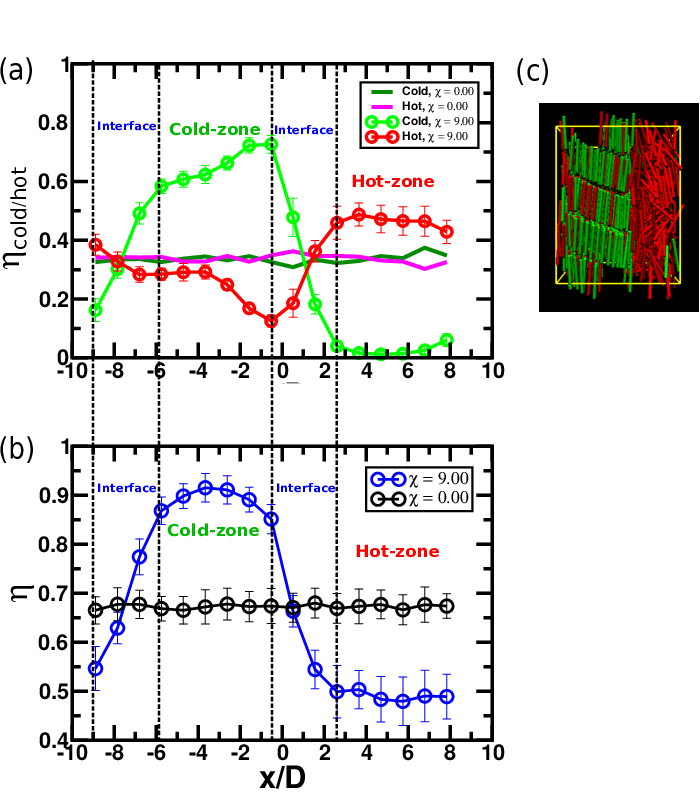
The effective temperature decreases continuously from hot to cold zone (Fig. 14-b). The coexistence of two temperatures at the hot-cold interface signifies the non-equilibrium nature of the system. However, it is surprising that in the steady state, the cold zone has regions where the local temperature is lower than the imposed cold particles’ temperature () and in some regions of the hot zone, local temperature is much higher than the imposed hot particles temperature (). In Fig. 14-b, we see that the maximum temperature in the hot zone is around 50 which is much higher than . In the cold zone, the minimum temperature is around 2 which is lower than . Though the effective temperature averaged over all the hot particles, , is lower than and the effective temperature averaged over all the cold particles, , is higher than due to heat exchange between them as mentioned in Eq-2.
We evaluate the pressure profile from diagonal components of the stress tensor.
| (7) |
| (8) |
| (9) |
Here, , , designate total, kinetic and virial pressures respectively. arises due to the particles’ interaction which is defined as the product of relative distance and interacting force between the SRS and . We observe that, the local pressure increases with activity and it is nearly constant within error bars across the hot-cold interface (Fig. 14-c). This is due to the fact that higher temperature causes higher kinetic pressure in the hot zone that acts at the hot-cold interface inducing higher packing and ordering in the cold zone. This enhances the virial pressure in the cold zone, resulting in the total pressure being constant across the interface. This is shown in figure 14-(c) where we decompose the total pressure into kinetic and virial part for the system with , . However, this behavior is found only for the lower densities (initial phases I, N). In the case of higher densities (initial phases Sm, K), we observe the total pressure decreases continuously from the hot to the cold zone (Fig. 15). This can be rationalized as follows: In the case of smectic and crystal initial phases, along with the kinetic pressure, virial pressure is also high in the hot zone due to their high orientational order ( as the hot zone shows nematic-like structure [Fig. 10, 11]). As a result total pressure increases in the hot zone which can not be compensated in the cold zone by increasing the virial pressure only. We calculate the pressure anisotropy () which is defined as:
| (10) |
Here, and are the normal and tangential components of the total pressure respectively along the direction perpendicular and parallel to the interface. We designate the perpendicular direction of the hot-cold interface as and the other 2 directions parallel to the interfacial plane as and . Thus the pressure components are defined as: and . In equilibrium, pressure is isotropic, and therefore, . In the active system, we observe that the anisotropy is close to zero within the error bars for lower densities (initial phases I, N). However, it increases for higher densities (initial phases Sm, K) as shown in Fig. 16-(a). To understand this precisely, we plot different pressure components across the interface as shown in Fig. 17 and find that the anisotropy in higher densities may arise due to the effect of active stress of the hot particles along their nematic director which acts parallel to the interfacial plane. To understand if the anisotropy in the pressure tensor is a consequence of the constant-volume simulation (NVT), we have done a constant-pressure simulation (NPT) with orthorhombic boundary condition and did not find a significant change in the pressure anisotropy. In references Dominguez et al. 2002; Bates and Luckhurst 1999; Hashim et al. 1995, it is reported that for equilibrium NPT simulation, the diagonal components of the pressure tensor become unequal in spatially ordered phases (smectic and crystal) due to maintaining a constant cubic shape throughout the simulation. In our case, NPT simulation is done in orthorhombic boundary conditions; hence this issue is not applicable in our case.
To understand possible system-size effects, we have done similar analysis with particles keeping all other system parameters and simulation protocol unchanged and we have not found any significant system size effect. The different results for two system sizes are compared in figure 19, 20 and 21 in the appendix.


IV Conclusions and Future outlook
In summary, we have presented a simple two-temperature model to study the thermodynamic and structural properties of active-passive spherocylinders where the level of activity is modeled by maintaining a temperature difference between the ‘hot’ and ‘cold’ particles. Starting from different initial equilibrium phases (I, N, Sm), we show that our simple model leads to not only phase separation into hot and cold regions but also liquid crystal ordering of the cold particles, and opposite shifts of the phase boundaries for mesophase formation, with respect to the equilibrium case, in the cold and hot domains. The extent of phase separation is quantified by an order parameter based on the local density. We find that the critical activity for phase separation lies in a small range, , for a wide range of densities from the isotropic to the crystal phase. This interesting observation highlights two-temperature model as an experimentally feasible system for studying effect of scalar activity in colloidal rods. We observe that the critical activity decreases with density in the liquid regime and increases again in the crystal regime. Based on these observations, a phase diagram is drawn in the state phase, vs. , showing the parametric regions of phase-separated and homogeneously mixed states.
We find the segregated zones developing different liquid crystal structures depending on the activity and initial phase of the system. For example, an initial isotropic configuration shows nematic ordering in the cold region, which eventually turns into crystalline ordering at higher activities. Similarly, an initial nematic configuration shows smectic or crystal ordering in the cold zone, depending on the value of , and isotropic structure in the hot zone. As a result, the I-N phase boundary shifts towards higher density for the hot particles and lower density for the cold particles. The segregated structures are identified by calculating the local nematic order parameter and different pair correlation functions. Finally, we analyse interfacial profiles of various thermodynamic quantities and conclude that the order-disorder transitions in the segregated zones are probably governed by local balance of pressure across the interface: higher temperature induces higher kinetic pressure in the hot zone which is compensated in the cold zone by an increased virial pressure.
Another possible reason for the order-disorder transition may be an entropic effect. The hot particles compensate for the loss of entropy due to ordering transition in the cold zone by developing a disordered structure. An important component of our future work will be to examine configurational entropy and free energy, as well as entropy production and currents, to shed light on the mechanisms underlying the nonequilibrium phase transitions we observe. Finally, analytical theories of two-temperature models are so far limited to spherical particles Grosberg and Joanny 2015; Grosberg and Joanny 2018; Ilker and Joanny 2020. Hence, generalizing their theoretical approach to make analytical predictions for two-temperature models with anisotropic particles is an important challenge.
Acknowledgements.
We would like to thank Aparna Baskaran for helpful discussions. We also thank Prof. Yves Lansac for insightful suggestion. We thank DAE, India for financial support through providing computational facility. JC acknowledges support through an INSPIRE fellowship. SR was supported by a J C Bose Fellowship of the SERB, India, and by the Tata Education and Development Trust, and acknowledges discussions during the KITP 2020 online program on Symmetry, Thermodynamics and Topology in Active Matter. This research was supported in part by the National Science Foundation under Grant No. NSF PHY-1748958. CD was supported by a Distinguished Fellowship of the SERB, India.References
- Marchetti et al. (2013) M. C. Marchetti, J. F. Joanny, S. Ramaswamy, T. B. Liverpool, J. Prost, M. Rao, and R. A. Simha, Rev. Mod. Phys. 85, 1143 (2013).
- Ramaswamy (2010) S. Ramaswamy, Annual Review of Condensed Matter Physics 1, 323–345 (2010).
- Romanczuk et al. (2012) P. Romanczuk, M. Bär, W. Ebeling, B. Lindner, and L. Schimansky-Geier, The European Physical Journal Special Topics 202, 1–162 (2012).
- Cates and Tailleur (2015) M. E. Cates and J. Tailleur, Annual Review of Condensed Matter Physics 6, 219 (2015).
- Ramaswamy et al. (2003) S. Ramaswamy, R. A. Simha, and J. Toner, Europhysics Letters (EPL) 62, 196–202 (2003).
- Toner et al. (2005) J. Toner, Y. Tu, and S. Ramaswamy, Annals of Physics 318, 170 (2005).
- Toner and Tu (1995) J. Toner and Y. Tu, Phys. Rev. Lett. 75, 4326 (1995).
- Toner and Tu (1998) J. Toner and Y. Tu, Phys. Rev. E 58, 4828 (1998).
- Buttinoni et al. (2013) I. Buttinoni, J. Bialké, F. Kümmel, H. Löwen, C. Bechinger, and T. Speck, Phys. Rev. Lett. 110, 238301 (2013).
- Bialké et al. (2015) J. Bialké, J. T. Siebert, H. Löwen, and T. Speck, Phys. Rev. Lett. 115, 098301 (2015).
- Bechinger et al. (2016) C. Bechinger, R. Di Leonardo, H. Löwen, C. Reichhardt, G. Volpe, and G. Volpe, Rev. Mod. Phys. 88, 045006 (2016).
- Mandal et al. (2019) S. Mandal, B. Liebchen, and H. Löwen, Phys. Rev. Lett. 123, 228001 (2019).
- Löwen (2020) H. Löwen, The Journal of Chemical Physics 152, 040901 (2020).
- Vutukuri et al. (2016) H. R. Vutukuri, Z. Preisler, T. H. Besseling, A. Van Blaaderen, M. Dijkstra, and W. T. Huck, Soft Matter 12, 9657 (2016).
- Redner et al. (2013) G. S. Redner, M. F. Hagan, and A. Baskaran, Phys. Rev. Lett. 110, 055701 (2013).
- Speck et al. (2014) T. Speck, J. Bialké, A. M. Menzel, and H. Löwen, Phys. Rev. Lett. 112, 218304 (2014).
- Saha et al. (2020) S. Saha, J. Agudo-Canalejo, and R. Golestanian, Phys. Rev. X 10, 041009 (2020).
- Tjhung et al. (2018) E. Tjhung, C. Nardini, and M. E. Cates, Phys. Rev. X 8, 031080 (2018).
- Stenhammar et al. (2015) J. Stenhammar, R. Wittkowski, D. Marenduzzo, and M. E. Cates, Phys. Rev. Lett. 114, 018301 (2015).
- Netz (2020) R. R. Netz, Phys. Rev. E 101, 022120 (2020).
- Chaki and Chakrabarti (2018) S. Chaki and R. Chakrabarti, Physica A: Statistical Mechanics and its Applications 511, 302 (2018).
- Chaki and Chakrabarti (2019) S. Chaki and R. Chakrabarti, The Journal of chemical physics 150, 094902 (2019).
- McCandlish et al. (2012) S. R. McCandlish, A. Baskaran, and M. F. Hagan, Soft Matter 8, 2527 (2012).
- Shaebani et al. (2020) M. R. Shaebani, A. Wysocki, R. G. Winkler, G. Gompper, and H. Rieger, Nature Reviews Physics 2, 181 (2020).
- Das (2017) S. K. Das, The Journal of chemical physics 146, 044902 (2017).
- Ganai et al. (2014) N. Ganai, S. Sengupta, and G. I. Menon, Nucleic acids research 42, 4145 (2014).
- Grosberg and Joanny (2015) A. Y. Grosberg and J.-F. Joanny, Phys. Rev. E 92, 032118 (2015).
- Grosberg and Joanny (2018) A. Y. Grosberg and J.-F. Joanny, Polymer Science, Series C 60, 118 (2018).
- Ilker and Joanny (2020) E. Ilker and J.-F. Joanny, Phys. Rev. Research 2, 023200 (2020).
- Weber et al. (2016) S. N. Weber, C. A. Weber, and E. Frey, Phys. Rev. Lett. 116, 058301 (2016).
- Smrek and Kremer (2017) J. Smrek and K. Kremer, Phys. Rev. Lett. 118, 098002 (2017).
- Smrek and Kremer (2018) J. Smrek and K. Kremer, Entropy 20, 520 (2018).
- Chari et al. (2019) S. S. N. Chari, C. Dasgupta, and P. K. Maiti, Soft matter 15, 7275 (2019).
- Bartnick et al. (2016) J. Bartnick, A. Kaiser, H. Löwen, and A. V. Ivlev, The Journal of chemical physics 144, 224901 (2016).
- Ivlev et al. (2015) A. V. Ivlev, J. Bartnick, M. Heinen, C.-R. Du, V. Nosenko, and H. Löwen, Phys. Rev. X 5, 011035 (2015).
- Soto and Golestanian (2014) R. Soto and R. Golestanian, Phys. Rev. Lett. 112, 068301 (2014).
- Schaller et al. (2010) V. Schaller, C. Weber, C. Semmrich, E. Frey, and A. R. Bausch, Nature 467, 73 (2010).
- Sumino et al. (2012) Y. Sumino, K. H. Nagai, Y. Shitaka, D. Tanaka, K. Yoshikawa, H. Chaté, and K. Oiwa, Nature 483, 448 (2012).
- De Gennes and Prost (1993) P.-G. De Gennes and J. Prost, The physics of liquid crystals, Vol. 83 (Oxford university press, 1993).
- Vicsek and Zafeiris (2012) T. Vicsek and A. Zafeiris, Physics reports 517, 71 (2012).
- Chaté et al. (2006) H. Chaté, F. Ginelli, and R. Montagne, Phys. Rev. Lett. 96, 180602 (2006).
- Mishra and Ramaswamy (2006) S. Mishra and S. Ramaswamy, Phys. Rev. Lett. 97, 090602 (2006).
- Peruani et al. (2006) F. Peruani, A. Deutsch, and M. Bär, Physical Review E 74, 030904(R) (2006).
- Weitz et al. (2015) S. Weitz, A. Deutsch, and F. Peruani, Phys. Rev. E 92, 012322 (2015).
- Ginelli et al. (2010) F. Ginelli, F. Peruani, M. Bär, and H. Chaté, Phys. Rev. Lett. 104, 184502 (2010).
- Huber et al. (2018) L. Huber, R. Suzuki, T. Krüger, E. Frey, and A. Bausch, Science 361, 255 (2018).
- Yang et al. (2010) Y. Yang, V. Marceau, and G. Gompper, Phys. Rev. E 82, 031904 (2010).
- Bott et al. (2018) M. C. Bott, F. Winterhalter, M. Marechal, A. Sharma, J. M. Brader, and R. Wittmann, Physical Review E 98, 012601 (2018).
- Simha and Ramaswamy (2002) R. A. Simha and S. Ramaswamy, Phys. Rev. Lett. 89, 058101 (2002).
- Hatwalne et al. (2004) Y. Hatwalne, S. Ramaswamy, M. Rao, and R. A. Simha, Phys. Rev. Lett. 92, 118101 (2004).
- Thampi et al. (2015) S. P. Thampi, A. Doostmohammadi, R. Golestanian, and J. M. Yeomans, EPL (Europhysics Letters) 112, 28004 (2015).
- Santhosh et al. (2020) S. Santhosh, M. R. Nejad, A. Doostmohammadi, J. M. Yeomans, and S. P. Thampi, Journal of Statistical Physics , 1 (2020).
- Maitra and Voituriez (2020) A. Maitra and R. Voituriez, Phys. Rev. Lett. 124, 048003 (2020).
- Weeks et al. (1971) J. D. Weeks, D. Chandler, and H. C. Andersen, The Journal of chemical physics 54, 5237 (1971).
- Allen et al. (1993) M. P. Allen, G. T. Evans, D. Frenkel, and B. Mulder, Advances in chemical physics 86, 1 (1993).
- Vega and Lago (1994) C. Vega and S. Lago, Computers & chemistry 18, 55 (1994).
- Earl et al. (2001) D. J. Earl, J. Ilnytskyi, and M. R. Wilson, Molecular physics 99, 1719 (2001).
- Heyes et al. (2015) D. M. Heyes, P. Turner, R. J. English, R. Williams, and A. C. Brańka, Phys. Rev. E 91, 042134 (2015).
- Cuetos et al. (2002) A. Cuetos, B. Martınez-Haya, L. Rull, and S. Lago, The Journal of chemical physics 117, 2934 (2002).
- Verlet (1967) L. Verlet, Physical review 159, 98 (1967).
- Omelyan (1998) I. P. Omelyan, Computers in Physics 12, 97 (1998).
- Martys and Mountain (1999) N. S. Martys and R. D. Mountain, Physical Review E 59, 3733 (1999).
- Rotunno et al. (2004) M. Rotunno, T. Bellini, Y. Lansac, and M. A. Glaser, The Journal of chemical physics 121, 5541 (2004).
- Maiti et al. (2002) P. K. Maiti, Y. Lansac, M. A. Glaser, and N. A. Clark, Physical review letters 88, 065504 (2002).
- Lansac et al. (2003) Y. Lansac, P. K. Maiti, N. A. Clark, and M. A. Glaser, Physical Review E 67, 011703 (2003).
- Berendsen et al. (1984) H. J. Berendsen, J. v. Postma, W. F. van Gunsteren, A. DiNola, and J. R. Haak, The Journal of chemical physics 81, 3684 (1984).
- Cuetos and Martínez-Haya (2015) A. Cuetos and B. Martínez-Haya, Molecular Physics 113, 1137 (2015).
- McGrother et al. (1996) S. C. McGrother, D. C. Williamson, and G. Jackson, The Journal of Chemical Physics 104, 6755 (1996).
- Bolhuis and Frenkel (1997) P. Bolhuis and D. Frenkel, The Journal of chemical physics 106, 666 (1997).
- Dominguez et al. (2002) H. Dominguez, E. Velasco, and J. Alejandre, Molecular Physics 100, 2739 (2002).
- Bates and Luckhurst (1999) M. Bates and G. Luckhurst, The Journal of chemical physics 110, 7087 (1999).
- Hashim et al. (1995) R. Hashim, G. Luckhurst, and S. Romano, Journal of the Chemical Society, Faraday Transactions 91, 2141 (1995).
*
Appendix A Quantifying macroscopic phase separation:
To quantify if the phase-separation happens in the macroscopic level, we have used the following critera: we divide the simulation box into a number of slabs () along the direction normal to the interface. is chosen such that each slab contains enough particles (in our case, about ) to get stable statistics. For each slab , we calculate the number difference of hot () and cold () particles divided by total number of particles () in that slab. We then define:
| (11) |
where represents a steady-state average over a sufficiently large number of configurations. The average of over all slabs will be 0 as varies symmetrically from to from the hot-rich to the cold-rich zone. We therefore calculate Fourier transformation of where measures the position of the slab. The magnitude of the first non-vanishing Fourier component is the measure of macroscopic phase separation in our system (Fig. 18). In Fig. 18-b, the 1st peak occurs at x = 31.42 which is approximately the length of our simulation box (L = 32). This indicates occurrence of phase separation in macroscopic scale. In Fig. 18-c, we plot the magnitude of for the smallest as a function of the activity at several packing fractions that shows similar trend as shown in Fig. 4 in the main text.


