When an Energy-Efficient Scheduling is Optimal for Half-Duplex Relay Networks?This research was supported in part by NSF under Award #1907785.

Computing the Shannon capacity of a wireless relay network is an open problem. In a half-duplex $n$-relay network, each relay can either transmit or receive at a given time instant and therefore a scheduling question arises: What fraction of time each relay in the network should be scheduled to receive/transmit information so that rates close to the Shannon capacity of the network can be achieved?

For an $n$-relay half-duplex network, there are $2^{n}$ possible receive/transmit configuration states, because each relay can either be scheduled for reception or transmission. However, in [1], it has been surprisingly shown that only $n+1$ out of these $2^{n}$ possible states are sufficient to achieve the network approximate capacity, i.e., an additive gap approximation of the Shannon capacity, where the gap is only a function of $n$. This result opens novel research directions, such as characterizing a set of $n+1$ critical states for each network efficiently (in polynomial time in $n$).

In this work, we investigate the question above in the context of diamond networks with $n$ interconnected relays, where the source communicates with the destination by hopping information through $n$ half-duplex relays that can communicate with each other. In particular, we analyze the linear deterministic approximation of the Gaussian noise channel, and characterize sufficient conditions under which at most one relay is required to transmit at any given time to achieve the approximate capacity. This leads to a significant reduction in the average power consumption at the relays, compared to a random network with identical $n$ (where potentially at each point in time more than one relay is transmitting) and hence, the proposed scheduling is energy-efficient. The other advantage of a schedule with at most one relay in transmit mode is that it simplifies the synchronization problem at the destination. Our result can be readily translated to obtain sufficient conditions under which operating the network only in states with at most one relay in receive mode is sufficient to achieve the approximate capacity. The proposed scheduling and approximate capacity can be translated to obtain similar results for the practically relevant Gaussian noise channel.

To the best of our knowledge, this is the first work that provides network conditions that suffice to characterize a set of $n+1$ critical states for arbitrary values of $n$ in relay networks where, in addition to broadcasting and signal superposition, we also have communicating/interconnected relays.

The Gaussian half-duplex diamond network with $n$ interconnected relays consists of a source (node $s$) that wishes to communicate with a destination (node $d$) through $n$ interconnected relays. At each time instant $t$, the input/output relationship of this network is described as

for $i\in[n]$. Note that, at each time instant $t$: (i) $S_{i}(t)$ is a binary random variable that indicates the state of relay $i\in[n]$, with $S_{i}(t)=0$ (respectively, $S_{i}(t)=1$) indicating that relay $i$ is receiving (respectively, transmitting); (ii) $X_{i}(t)$ is the channel input at node $i$ that satisfies the unit average power constraint $\mathbb{E}[|X_{i}(t)|^{2}]\leq 1$ for $i\in\{s\}\cup[n]$; (iii) $h_{ij}$ with $i\in[n]\cup\{d\}$ and $j\in\{s\}\cup[n]$ is the time-invariant complex channel gain from node $j$ to node $i$; note that $h_{ds}=0$ and, since the relays operate in half-duplex mode, without loss of generality we let $h_{ii}=0$; (iv) $Z_{i}(t)\sim\mathcal{CN}(0,1)$ is the complex additive white Gaussian noise at node $i\in\{d\}\cup[n]$; and finally, (v) $Y_{i}(t)$ is the received signal at node $i\in\{d\}\cup[n]$.

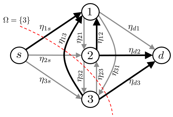
The Shannon capacity $\mathsf{C}^{\text{G}}$ of the network in (1) is not known for general $n$. However, the capacity can be approximated within a constant $O(n)$ bit gap. More precisely, we can focus on the binary linear deterministic approximation of the Gaussian noise network model [2], for which the approximate capacity is known and provides an approximation for $\mathsf{C}^{\text{G}}$. The linear deterministic model (a.k.a. ADT model [2]) corresponding to the Gaussian noise network in (1) has an input-output relationship given by

for $i\in[n]$, where

and

Here, the vectors $X_{s}(t)$, $X_{i}(t)$, $Y_{d}(t)$, and $Y_{i}(t)$ with $i\in[n]$ are binary of length $\eta=\max\eta_{ij}$, where the maximization is taken over all channels $\eta_{ij}$’s in the network; ${\mathbf{D}}$ is the so-called $\eta\times\eta$ shift matrix, and $S_{i}(t),i\in[n]$ is the $i$th relay binary-valued state random variable.

The approximate capacity of the linear deterministic model in (2) is given by the solution of

where: (i) $\mathcal{S}=\{i\in[n]:S_{i}=1\}$ is the set of relay nodes in transmit mode; (ii) $\lambda_{\mathcal{S}}\geq 0$ is the fraction of time that the network operates in state $\mathcal{S}$ and hence, $\sum_{\mathcal{S}\subseteq[n]}\lambda_{\mathcal{S}}{\leq}1$; (iii) $\bm{\lambda}$ is referred to as a network schedule and is a vector obtained by stacking together $\lambda_{\mathcal{S}}$ for all $\mathcal{S}\subseteq[n]$; (iv) $\Omega\subseteq[n]$ denotes a partition of the relays in the ‘side of $s$’, i.e., $\{s\}\cup\Omega$ is a network cut; similarly, $\Omega^{c}=[n]\setminus\Omega$ is a partition of the relays in the ‘side of $d$’. Moreover, we define

where $\mathbf{F}^{\Omega}_{\mathcal{S}}$ is the transfer matrix from $X_{\{s\}\cup(\Omega\cap\mathcal{S})}$ to $Y_{\{d\}\cup(\Omega^{c}\cap\mathcal{S}^{c})}$, corresponding to the ADT model [2].

It turns out that $|\mathsf{C}^{\text{G}}-\mathsf{C}^{\text{LD}}|\leq\kappa$, where $\kappa=O(n)$ is independent of the channel gains and operating SNR and hence, $\mathsf{C}^{\text{LD}}$ in (3) provides an approximation for the Shannon capacity of the network in (1)¹¹ 1 We highlight that schemes such as quantize-map-and-forward [2] and noisy network coding [4], together with the cut set bound, allow to characterize the capacity of Gaussian relay networks up to a constant additive gap..

Therefore, we have

In this work, we seek to identify sufficient network conditions which allow to determine a set of $n+1$ states (out of the $2^{n}$ possible ones) that suffice to achieve the approximate capacity in (3) of the linear deterministic network and can be readily translated into a similar result for the original noisy Gaussian channel model in (1).

Without loss of generality, we assume that the relay nodes are arranged in increasing order of their left link capacities, that is, $\eta_{1s}\leq\eta_{2s}\leq\dots\leq\eta_{ns}$. We define $\mathbf{P}$ to be an $(n+2)\times(n+2)$ matrix, the rows and columns of which are indexed by $[0:n+1]$, and

where we define $f^{\Omega}_{\{n+1\}}=f^{\Omega}_{\varnothing}$, for consistency. Moreover, for $i\in[0:n+1]$ we use $\mathsf{P}_{(i)}$ to denote the minor of $\mathbf{P}$ associated with the row $0$ and column $i$ of the matrix $\mathbf{P}$, that is

Finally, we define

to be the set of the $n+1$ states, where at most one relay is transmitting in each state.

The main result of this paper is presented in Theorem 1, which characterizes sufficient network conditions for the optimality of operating the network only in states $\mathcal{S}\in\mathbb{S}$.

In the remainder of this section, we analyze the variables $f^{\Omega}_{\mathcal{S}}$ and present some of their properties, which play an important role in the proof of Theorem 1, presented in Section IV.

In this section, we present the proof of Theorem 1, which consists of three main steps. We first introduce an auxiliary optimization problem in (9) in Section IV-A, which is a relaxed version of the problem in (3) and hence, its solution $\mathsf{C}^{\text{U}}$ provides an upper bound on the optimum value of (3), i.e., $\mathsf{C}^{\text{U}}\geq\mathsf{C}^{\text{LD}}$. In Section IV-B, we propose a solution $(\bm{\lambda}^{\star},t^{\star})$ for the (relaxed) optimization problem in (9), where ${\lambda}^{\star}_{\mathcal{S}}=0$ for all $\mathcal{S}\notin\mathbb{S}$. We show that, under the conditions of Theorem 1, $(\bm{\lambda}^{\star},t^{\star})$ is feasible and optimal, which leads to $\mathsf{C}^{\text{U}}=t^{\star}$. Finally, in Section IV-C we show that the proposed solution is feasible for the original problem in (3), implying that $\mathsf{C}^{\text{LD}}\geq t^{\star}$. Therefore, putting the three results together, we get $t^{\star}=\mathsf{C}^{\text{U}}\geq\mathsf{C}^{\text{LD}}\geq t^{\star}$. This shows that $\mathsf{C}^{\text{LD}}=t^{\star}$ can be attained by $\bm{\lambda}^{\star}$ that satisfies the claim of Theorem 1. This concludes the proof of the theorem.

References

- [1] M. Cardone, D. Tuninetti, and R. Knopp, “On the optimality of simple schedules for networks with multiple half-duplex relays,” IEEE Trans. Inf. Theory, vol. 62, no. 7, pp. 4120–4134, July 2016.
- [2] A. S. Avestimehr, S. N. Diggavi, and D. N. C. Tse, “Wireless network information flow: A deterministic approach,” IEEE Trans. Inf. Theory, vol. 57, no. 4, pp. 1872–1905, April 2011.
- [3] A. Özgür and S. N. Diggavi, “Approximately achieving Gaussian relay network capacity with lattice-based QMF codes,” IEEE Trans. Inf. Theory, vol. 59, no. 12, pp. 8275–8294, December 2013.
- [4] S. Lim, Y.-H. Kim, A. El Gamal, and S.-Y. Chung, “Noisy network coding,” IEEE Trans. Inf. Theory, vol. 57, no. 5, pp. 3132 –3152, 2011.
- [5] S. H. Lim, K. T. Kim, and Y. H. Kim, “Distributed decode-forward for multicast,” in IEEE International Symposium on Information Theory (ISIT), June 2014, pp. 636–640.
- [6] M. Cardone, D. Tuninetti, R. Knopp, and U. Salim, “Gaussian half-duplex relay networks: improved constant gap and connections with the assignment problem,” IEEE Trans. Inf. Theory, vol. 60, no. 6, pp. 3559 – 3575, June 2014.
- [7] H. Bagheri, A. S. Motahari, and A. K. Khandani, “On the capacity of the half-duplex diamond channel,” in 2010 IEEE International Symposium on Information Theory, 2010, pp. 649–653.
- [8] S. Jain, M. Cardone, and S. Mohajer, “Operating half-duplex diamond networks with two interfering relays,” in IEEE Information Theory Workshop (ITW), July 2021.
- [9] Y. H. Ezzeldin, M. Cardone, C. Fragouli, and D. Tuninetti, “Efficiently finding simple schedules in Gaussian half-duplex relay line networks,” in IEEE International Symposium on Information Theory (ISIT), June 2017, pp. 471–475.
- [10] R. H. Etkin, F. Parvaresh, I. Shomorony, and A. S. Avestimehr, “Computing half-duplex schedules in Gaussian relay networks via min-cut approximations,” IEEE Trans. Inf. Theory, vol. 60, no. 11, pp. 7204–7220, November 2014.
- [11] S. Jain, M. Elyasi, M. Cardone, and S. Mohajer, “On simple scheduling in half-duplex relay diamond networks,” in IEEE International Symposium on Information Theory (ISIT), July 2019.