Building robust AGN mock catalogs to unveil black hole evolution and for survey planning
Abstract
The statistical distributions of active galactic nuclei (AGN), i.e. accreting supermassive black holes (BHs), in mass, space and time, are controlled by a series of key properties, namely the BH-galaxy scaling relations, Eddington ratio distributions and fraction of active BH (duty cycle). Shedding light on these properties yields strong constraints on the AGN triggering mechanisms whilst providing a clear baseline to create useful “mock” catalogues for the planning of large galaxy surveys. We here delineate a robust methodology to create mock AGN catalogs built on top of large N-body dark matter simulations via state-of-the-art semi-empirical models. We show that by using as independent tests the AGN clustering at fixed X-ray luminosity, galaxy stellar mass and BH mass, along with the fraction of AGN in groups and clusters, it is possible to significantly narrow down the choice in the relation between black hole mass and host galaxy stellar mass, the duty cycle, and the average Eddington ratio distribution, delivering well-suited constraints to guide cosmological models for the co-evolution of BHs and galaxies. Avoiding such a step-by-step methodology inevitably leads to strong degeneracies in the final mock catalogs, severely limiting their usefulness in understanding AGN evolution and in survey planning and testing.
Subject headings
Surveys - Galaxies: active - X-rays: general - Cosmology: Large-scale structure of Universe - Dark MatterI. Introduction
Several semi-analytical models and hydrodynamical simulations (Springel et al. 2005; Hopkins et al. 2006; Menci et al. 2008, e.g.) have been developed in recent years to describe the main mechanisms that fuel the central supermassive black holes (BHs). With suitable adjustment of parameters, these models can explain many aspects of AGN phenomenology (Hopkins et al. 2006; Hopkins et al. 2008, e.g.). Often relying on a rather heavy parameterization of the physics regulating the cooling, star formation, feedback, and merging of baryons (Monaco et al. 2007, e.g.), semi-analytic models of galaxy evolution can present serious degeneracies (González et al. 2011; Lapi et al. 2018, e.g.), or even significant divergences in, e.g., the adopted sub-grid physics (Scannapieco et al. 2012; Nuñez-Castiñeyra et al. 2020). Semi-empirical models (SEMs) represent an original and complementary methodology to more traditional modelling approaches (Hopkins & Hernquist 2009, e.g.). The aim of SEMs is to tackle specific aspects of galaxy and BH evolution in a transparent, fast, and flexible way, relying on just a few input assumptions and parameters. SEMs cannot replace ab-initio models of galaxy and BH evolution but can provide guidance to reduce the space of parameters and shed light on the viable physical processes.


It is particularly relevant the application of SEMs to the creation of active and normal galaxy “mock” catalogues (Conroy & White 2013, e.g.), which are a vital component of the planning of imminent extra-galactic surveys such as Euclid (Laureijs et al. 2011) and the Vera C. Rubin Observatory Legacy Survey of Space and Time (LSST Science Collaboration et al. 2009, LSST;). The first step for the creation of mocks consists in assigning galaxies to dark matter halos extracted from large cosmological N-body simulations (Riebe et al. 2013; Klypin et al. 2016, e.g.), via abundance-matching techniques (Kravtsov et al. 2004; Vale & Ostriker 2004; Shankar et al. 2006; Behroozi et al. 2013a; Moster et al. 2013, e.g.). Despite being based on minimal assumptions, the latter are not immune to important systematics, mostly related to the input data, which propagate onto the star formation and mass assembly histories predicted by SEMs (Grylls et al. 2020b; Grylls et al. 2020a; O’Leary et al. 2020, e.g.).
In the last few years, several studies have focused on the creation of mock catalogs specifically for AGN that can be utilized for the planning and testing of large-scale AGN-dedicated extragalactic surveys such eROSITA (Georgakakis et al. 2019; Comparat et al. 2019; Aird & Coil 2020, e.g.). These AGN mocks are built by starting from an empirical galaxy catalog and by assigning to each object a specific accretion-rate that is proportional to the quantity , drawn randomly from observationally determined probability distributions (Bongiorno et al. 2016; Georgakakis et al. 2017; Aird et al. 2018, e.g.). This quantity can be measured directly from observations and provides an estimate of X-ray emission per unit stellar mass for a galaxy.

The advantage of this methodology is that by using just a few input relations, namely the stellar mass-halo mass relation (from abundance matching) and the probability distribution of specific accretion-rate , it allows to create a mock catalog of AGN that – by design – reproduces the observed X-ray luminosity function (XLF) and broadly matches the large-scale bias at a given host galaxy stellar mass. Using this approach, Georgakakis et al. 2019 populated cosmological simulations with AGN and showed that their clustering properties (including the signal at small scales), are consistent with state-of-the-art observational measurements of X-ray or UV/optically selected samples at different redshifts and accretion luminosities, supporting the view that the large-scale distribution of AGN may be independent of the detailed physics of BH fueling. Some recent works also tested the same methodology against the large-scale bias dependence on the X-ray luminosity at different redshifts (Georgakakis et al. 2019; Aird & Coil 2020).
However, in these models key information such as BH mass is largely bypassed, and the AGN duty cycle (i.e. the probability for a galaxy of being active above a certain luminosity or threshold) is not considered as a separate model input parameter, limiting the efficacy of these models in shedding light on the processes controlling the co-evolution of BHs and their hosts. Moreover, in these models the assignment of specific accretion-rates to mock galaxies by using is a stochastic process, assumed to be independent of the environment (centrals and satellites of similar stellar mass share the same probability of being active).
In this paper instead, we create mock catalogs of AGN by varying different input model parameters, namely the stellar mass–halo mass and BH mass–stellar mass relations, the AGN duty cycle, the Eddington ratio distribution and the fraction of satellite AGN (controlled by the parameter defined later) and test the effect on several observables, such as the AGN XLF, the distribution and AGN large-scale bias as a function of BH/stellar mass and luminosity. More generally, we demonstrate in this study that by calibrating the AGN mocks on the bias at fixed BH mass, stellar mass, and AGN luminosity, provides a self-consistent and robust route to break the most relevant degeneracies and narrow down the choice of input parameters. For example, Shankar et al. 2020 emphasized that current measurements of AGN clustering at (Krumpe et al. 2015) are already sufficient to constrain, in ways independent of the AGN duty cycle, the scaling relations of BHs (Kormendy & Ho 2013; Reines & Volonteri 2015; Savorgnan & Graham 2016; Shankar et al. 2016; Davis et al. 2018, e.g.). The main goal of this paper is to provide a complete framework to build a robust and realistic AGN mock catalog, consistent with many different and independent observables, and physically sound, being based on the underlying scaling relations between BHs and their host galaxies and dark matter halos.

II. Research Methodology
In this Section we provide the step-by-step description of our baseline methodology:
- •
At a given redshift of reference, in this work , we extract large catalogs of DM halos and subhalos from large, N-body dark matter simulations. We here rely on the MultiDark simulation (Riebe et al. 2013). The catalogues contain both central/parent halos and satellite halos with unstripped mass at infall.
- •
To each parent halo a central galaxy is assigned with stellar mass given by abundance matching relations at the redshift of reference (Grylls et al. 2019, e.g.), while satellite halos are assigned a stellar mass at their redshift of infall.
- •
To each galaxy we assign a BH mass from an empirical BH mass-galaxy mass relation drawn from several recent studies (Shankar et al. 2016, e.g.).
- •
To each galaxy and BH we then assign an Eddington ratio , with the bolometric luminosity and the Eddington limit of the BH. The parameter is randomly extracted from a distribution described by a Schechter function, the latter chosen in a way to reproduce the AGN XLF at , for a given input “duty cycle” (see below). In our reference model we ignore, for simplicity, any mass dependence of on, e.g., BH mass. We will discuss in Section V the (moderate) impact of relaxing this assumption. Regardless, we note that any mass dependence in is degenerate with the duty cycle (Shankar et al. 2013, e.g. in the AGN XLF;), a model input parameter which we explore thoroughly in this work.
- •
To each galaxy/BH an extinction corrected X-ray luminosity in the 2-10 keV band is then assigned from the bolometric luminosity via up-to-date bolometric corrections (Duras et al. 2020, e.g.).
- •
Each galaxy and its associated BH is assigned a duty cycle, i.e. a probability for a BH of a given MBH of being active, following empirically-based duty cycles (Man et al. 2019, e.g.).
We then generate our mock catalog of AGN and, by varying our input parameters, test a number of outputs, such as the AGN XLF, the AGN specific accretion-rate distribution and the AGN large-scale clustering. We focus on where the galaxy-BH scaling relations are better constrained and additional measurements on some of the key observables, such as AGN-galaxy clustering, are available. We stress that the methodology we put forward in this work is applicable to any redshift of interest. In Viitanen et al. (submitted), for example, we apply our methodology to , while in Carraro et al. (submitted) we push our methodology up to , and specifically focus on the correlation with star formation rate, which is not explicitly included in the present work.

II.1. Connecting halos to galaxies and BHs
We start from a large catalog of dark matter halos and subhalos from MultiDark11 1 www.cosmosim.org-Planck 2 (Riebe et al. 2013, MDPL2;) at the redshift z = 0.1. MDPL2 currently provides the largest publicly available set of high-resolution and large volume N-body simulations (box size of 1000 h-1Mpc, mass resolution of 1.51109 h-1M⊙). The ROCKSTAR halo finder (Behroozi et al. 2013b) has been applied to the MDPL2 simulations to identify halos and flag those (sub-halos) that lie within the virial radius of a more massive host halo. The mass of the dark matter halo is defined as the virial mass in the case of host halos and the infall progenitor virial mass for sub-halos.
From abundance matching techniques one can infer the stellar mass–halo mass relation which shows that the baryons are converted into stars with very different efficiencies in halos of diverse mass (Shankar et al. 2006; Moster et al. 2013, e.g.). We adopt the parameterization for the stellar-to-halo mass ratio by Moster et al. 2013:
| (1) |
where is the normalization of the stellar-to-halo mass ratio, a characteristic mass where the ratio is equal to the normalization , and two slopes and which indicate the behavior at low and high-halo mass ends, respectively. We fixed these redshift-dependent parameters as in Grylls et al. 2019 who suggested a steeper slope than Moster et al. 2013 for the high-mass end (Shankar et al. 2014; Shankar et al. 2017; Kravtsov et al. 2018, as also shown in), which better fits the SDSS-DR7 from Meert et al. 2015; Meert et al. 2016, with improved galaxy photometry 22 2 We decrease by 0.1 dex the original stellar masses by Grylls et al. 2019 to further improve the match to the latest stellar mass function by Bernardi et al. 2017..
Figure 1 (left panel) shows the stellar mass functions at presented in Bernardi et al. 2017, based on Sérsic-exponential fits to the surface brightness profiles of galaxies in the Sloan Digital Sky Survey (SDSS) Data Release 7 (DR7), and characterized by a significantly higher number densities of massive galaxies ( M∗) when compared to estimates by, e.g., Baldry et al. 2012; Moustakas et al. 2013; Bernardi et al. 2010; Bell et al. 2003.


II.2. Input MBH-Mstar relation
As a second step, to each galaxy we assign a BH mass assuming the following two scaling relations:
- •
The BH mass–stellar mass relation as derived in Shankar et al. 2016, labelled as BHSMR-Sha16 “debiased” hereafter:
(2) with a mass-dependent intrinsic scatter given by:
(3) as presented in Equation 5 of Shankar et al. 2019. Note that this equation is applicable to galaxies with stellar masses log M;
- •
the relation derived for the Savorgnan & Graham 2016 sample of galaxies with dynamically measured BH masses, BHSMR-SG16 (raw) hereafter, as presented in Equation 3 of Shankar et al. 2019, with a scatter of 0.5 dex:
(4)
The right panel of Figure 1 shows the MBH-Mstar relations defined by Equations 2 and 4 with their associated dispersions and compared with several other relations from the recent literature, as labelled. It can be seen from Figure 1 that our two chosen relations bracket the systematic uncertainties in both slope and normalization present in the local BH mass-galaxy stellar mass relation.
In our reference models throughout we include the scatters in the relations described above as random normal dispersions. However, it may be possible that some correlation between, in particular, the dispersions in BH mass and galaxy stellar mass at a given DM halo mass may exist. We thus explore in sec V some of the main consequences on our results of including a degree of covariance in the scatters, and refer to Viitanen et al. (submitted) for a more comprehensive discussion of implementing a covariant scatter in the input stellar mass–halo mass and BH mass–stellar mass relations.
II.3. Input Eddington ratio distribution
To each galaxy and BH we assign an Eddington ratio following a ) distribution described by:
- •
a Schechter function:
(5) with in the range = 10-4 – . The Schechter function is characterized by two free parameters: the knee , where the power-law form of the function cuts off and the power-law index . The Schechter function is supported by recent studies on the specific accretion-rate distribution of AGN, such as Bongiorno et al. 2016; Aird et al. 2017; Aird et al. 2018; Aird et al. 2019; Georgakakis et al. 2017.
- •
a Gaussian function:
(6) where varies in the range log = - 4 – 1, is the standard deviation and is the mean of the distribution.
Both the Schechter and Gaussian input are normalized to unity. Such Eddington ratio distributions have a lower cutoff at = below which the sources are no longer regarded as AGN. We choose to be low enough to include even the faintest AGN recorded in the AGN XLF, down to erg/s for BHs with mass . We note that the exact choice of is not too relevant in our modelling. By lowering/increasing would simply correspond to a higher/lower duty cycle, i.e. a higher/lower probability for BHs to active. In Sec. V we explore the effect on our results of assuming an input BH mass dependent Eddington ratio distribution, i.e. .
We then assign a bolometric luminosity to each source according to the Eddington ratio and the BH mass. The bolometric luminosity is then converted into intrinsic rest-frame 2-10 keV X-ray luminosity via the relation with the bolometric correction expressed as
| (7) |
with a = 10.96, b = 11.93, c = 17.79 (Duras et al. 2020).
II.4. Input BH duty cycle
In general terms, the total accretion probability of a BH to be active at a given Eddington ratio is a convolution of the duty cycle , i.e. the probability of a galaxy/BH to active as an AGN above a certain luminosity threshold, and the (normalized) Eddington ratio distribution ) of being accreting at a given rate (Steed & Weinberg 2003; Marconi et al. 2004; Aversa et al. 2015, e.g.). We here follow the rather common and broad approximation followed in the continuity equation formalism of expressing the total accretion probability into a simple product of the duty and the Eddington ratio distribution (Small & Blandford 1992; Marconi et al. 2004; Shankar et al. 2009, e.g.). This choice is extremely flexible and allows to disentangle the roles of a mass- and/or time-dependent duty cycle from an evolving characteristic Eddington ratio (Shankar et al. 2013, e.g.).
Both the Eddington ratio distribution ) and duty cycle have been separately studied by different groups. For the duty cycle in particular, despite the numerous dedicated works, no clear trend has yet emerged and controversial results are present in the literature. For this reason, we decided to test three different duty cycles for BHs with mass as shown is Figure 2:
- •
A duty cycle decreasing with BH mass, as derived in Schulze & Wisotzki 2010 at for Compton thin un/obscured AGN, labelled as U-SW10 (decr) hereafter;
- •
A duty cycle increasing with BH mass in a way to reproduce the increasing trend with host galaxy stellar mass as estimated at low redshift (z) by Man et al. 2019 for Narrow Line AGN in host galaxies with , U-M19 (incr) hereafter;
- •
A constant duty cycle , as suggested by Goulding et al. 2010, U-G10 (const) hereafter.
In all cases we define as duty cycle the probability of BHs to be active above the minimal Eddington ratio threshold in our input distribution. It is worth noticing that we are assuming that the duty cycle from Man et al. 2019 can be applied to both obscured and unobscured AGN. Given that it has been derived by using a sample of Narrow Line AGN, we can consider it as a lower limit. However, a similar duty cycle increasing with stellar mass has also been derived in Georgakakis et al. 2017 from a sample of Compton thin un/obscured AGN.
| log (or log) | ( or ) | log | |||
|---|---|---|---|---|---|
| Sha16 (Debiased) | Schulze & Wisotzki 2010 | Schechter | -0.45 | 0.15 | 31.81 |
| Sha16 (Debiased) | Man et al. 2019 | Schechter | -1.8 | -0.15 | 31.56 |
| Sha16 (Debiased) | Goulding et al. 2010 | Schechter | -1.9 | 0 | 31.56 |
| SG16 (Raw) | Schulze & Wisotzki 2010 | Schechter | -1.3 | -0.35 | 32.93 |
| SG16 (Raw) | Man et al. 2019 | Schechter | -2.5 | 0.4 | 31.8 |
| SG16 (Raw) | Goulding et al. 2010 | Schechter | -2.4 | 0.8 | 31.42 |
| Sha16 (Debiased) | Schulze & Wisotzki 2010 | Gaussian | -2.8 | 1 | 31.69 |
| Sha16 (Debiased) | Man et al. 2019 | Gaussian | -4 | 1 | 31.51 |
| Sha16 (Debiased) | Goulding et al. 2010 | Gaussian | -4 | 1.1 | 31.24 |
| SG16 (Raw) | Schulze & Wisotzki 2010 | Gaussian | -3 | 1.1 | 32.62 |
| SG16 (Raw) | Man et al. 2019 | Gaussian | -4.5 | 1.3 | 31.71 |
| SG16 (Raw) | Goulding et al. 2010 | Gaussian | -4.5 | 1.4 | 31.41 |
II.5. The Q parameter
The AGN duty cycle is the average fraction of both central and satellite galaxies to be active at a given stellar or BH mass, above a given threshold. However, the relative probability for a central and satellite BH to be active could still be different. To allow for this possibility, following Shankar et al. 2020 we define the total duty cycle as the sum of central and satellite at a given BH mass to be active, i.e. , with and the duty cycles of, respectively, satellite and central galaxies above a given luminosity or Eddington ratio threshold. We can then define the parameter as the relative probability of satellite and central AGN of being active. Constraining the parameter would be of course of key importance to shed light on the different AGN triggering mechanisms. For example, a high value of would point towards satellites being preferentially active rather than centrals of similar mass, a condition that would be difficult to reconcile with a strict merger-only scenario but possibly still consistent with disc instability processes (Gatti et al. 2016, e.g.).
Previous studies in the literature always assumed = 1 (Allevato et al. 2019; Shankar et al. 2020, noticeable exceptions are), implying that all central and satellite galaxies share equal probabilities of being active (Comparat et al. 2019; Aird & Coil 2020, e.g.). The parameter can in principle be directly measured from the fraction of satellite galaxies in groups and clusters of galaxies (see Gatti et al. 2016, and references therein). In fact the parameter can be expressed in terms of as , where is the total fraction of (active and non active) BHs in satellites with BH mass within and (Shankar et al. 2020, for full details, see).
III. Outputs
We then consider different outputs of our mock catalog of galaxies and BHs at a given z:
- •
The AGN X-ray luminosity function (XLF):
(8)
where = is the total (active and non active) BH mass function, is the AGN duty cycle, is the normalized Eddington ratio distribution with .
- •
The specific accretion rate distribution:
(9)
where defines the rate of accretion onto the central BH scaled relative to the stellar mass of the host galaxy. describes the probability of a galaxy to host an AGN of a given at a given redshift. We can also define the characteristic of the specific accretion-rate distribution as:
| (10) |
At variance with many other previous approaches, our flexible methodology based on an input duty cycle and Eddington ratio distribution allow us to use the distribution as an output rather than an input of our AGN mock catalog, thus providing an additional valuable constraint independent of AGN clustering. We will show that the distribution is particularly useful in constraining the viable duty cycles and also the underlying BH-galaxy scaling relations.
- •
The large-scale bias of mock AGN with BH mass (and similarly stellar mass) in the range and following the formalism of Shankar et al. 2020:
| (11) |
where is the duty cycle of central AGN, is the duty cycle of satellite AGN and is the number of central and satellite galaxies, in the BH mass bin and .


IV. Results
IV.1. AGN XLF and
We now use the model described in the previous section to create mock catalogs of AGN. We vary the input parameters and study how these changes affect the outputs, such as the AGN XLF and the specific accretion-rate distribution . We consider various different cases, and each combination of model input parameters are shown in Table 1.
We estimate the XLF (defined in equation 8) for the different duty cycles, setting the free parameters of the input ) distribution in order to reproduce the observationally inferred XLF of X-ray selected AGN at z = 0.1 (Miyaji et al. 2015). We infer the parameters of ) based on an overall match to an observational constraint, i.e. the AGN XLF, but we do not attempt formal - minimization because the errors themselves are not well defined enough to do so. We note where models fit observations within a plausible range of systematic uncertainties, and where they do not. Our objective is to show how the different ‘observables’ depend on the input model parameters and delineate a guideline for the creation of realistic AGN mock catalogs, so we are not inherently interested in the free parameters of ) that might better fit the (real) observations.
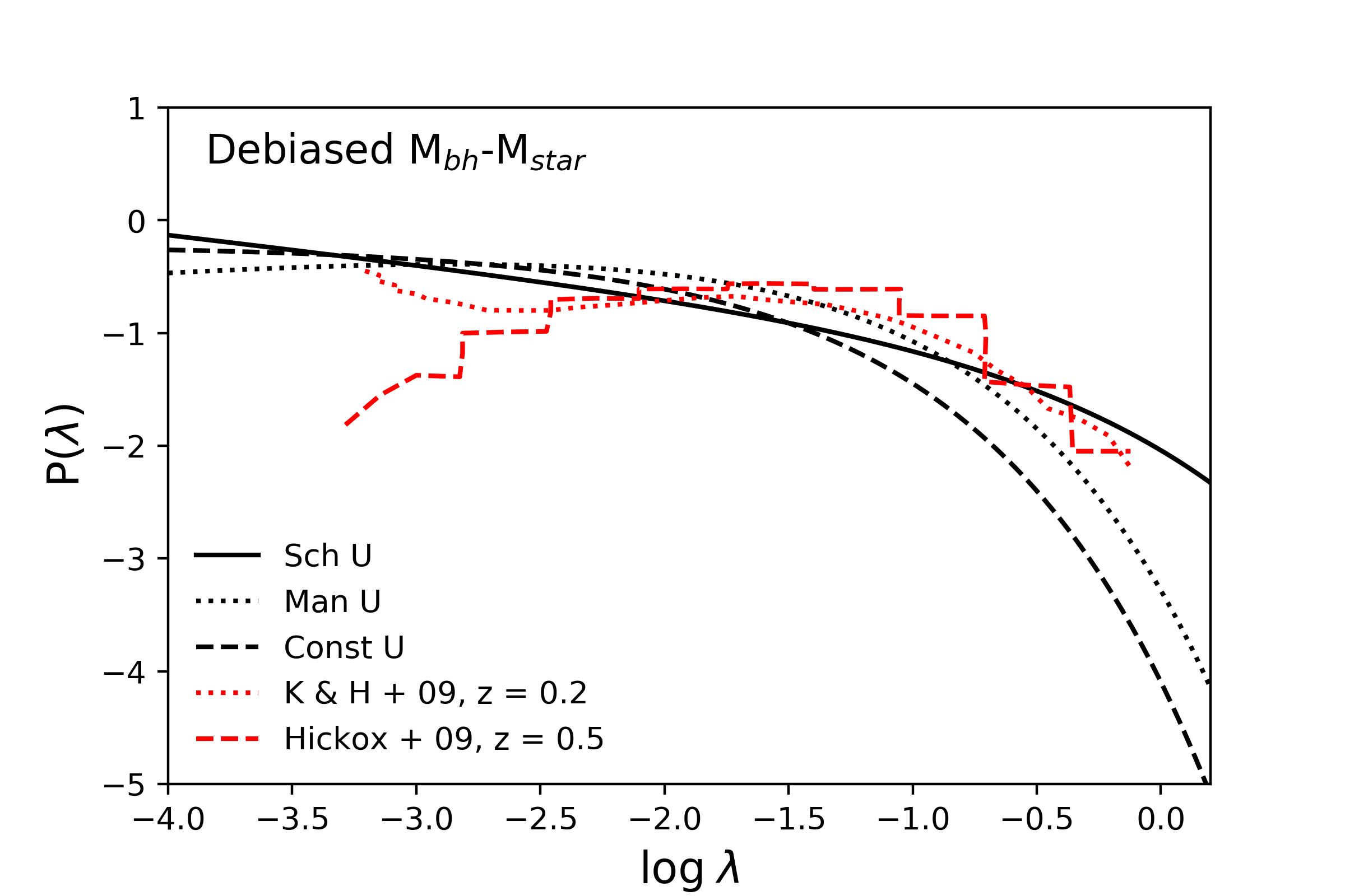
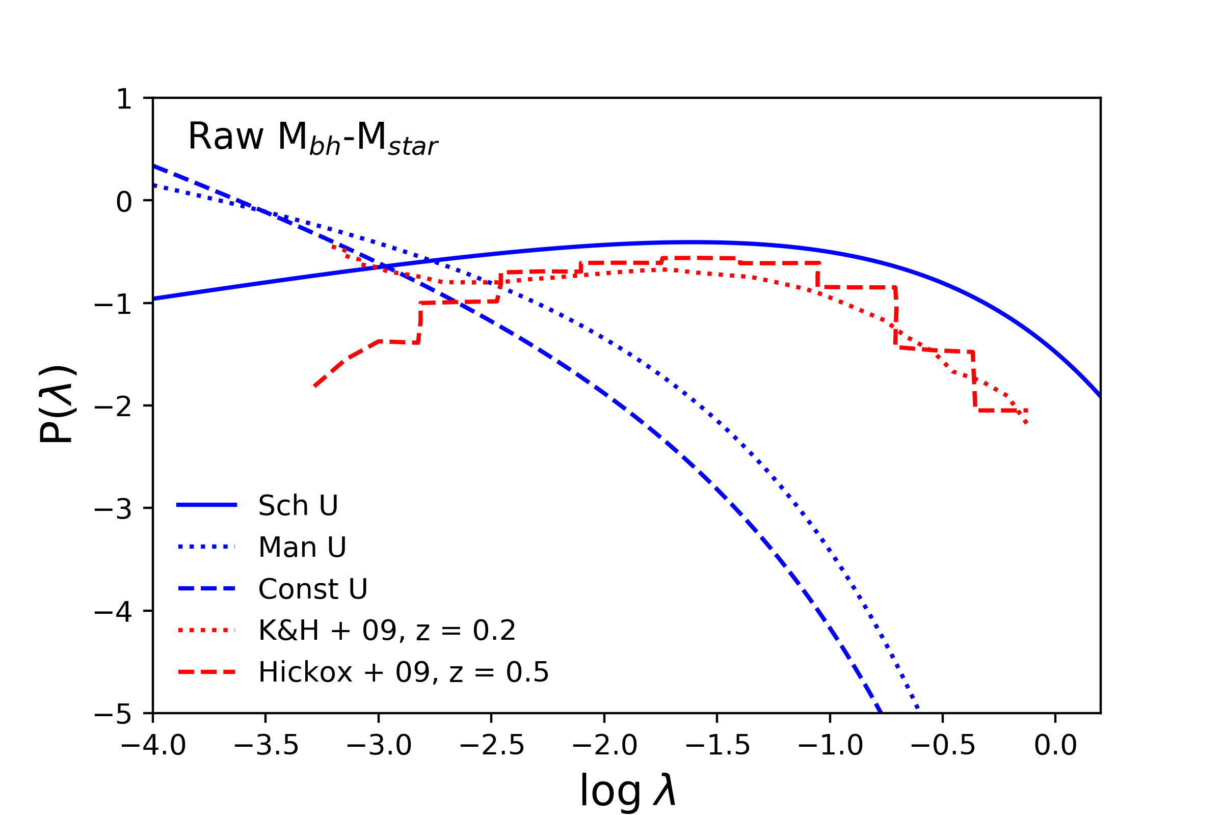
As a first case, we consider a ) described by a Schechter function. As shown in Figures 3 and 4, we can reproduce the observed AGN XLF as derived in Miyaji et al. 2015 for AGN at z = 0.1 (Ueda et al. 2014, or similarly in), independently of the choice of the input AGN duty cycle and BH mass–stellar mass relation. In particular, if we assume BHSMR-Sha16 (debiased), the input ) is characterised by a power-law index , i.e. an almost constant probability as a function of Eddington ratio at . Assuming the AGN duty cycle U-SW10 (decr), the input ) is almost consistent with observations (Kauffmann & Heckman 2009; Hickox et al. 2009, i.e.) with a knee log = - 0.45. It is worth noting that these observations are calibrated on the relation of Tremaine et al. (2002) that would shift the Eddington ratio distribution to higher by a factor of 2, still in agreement with our AGN mock predictions. A smaller knee (log -2) is obtained for mock AGN assuming U-M19 (incr) and U-G10 (const). Similarly, we can reproduce the observed AGN XLF for different AGN duty cycles when assuming SG16 (raw) (see figure 4). However, the corresponding input ) distributions of mock AGN with U-M19 (incr) and U-G10 (const) are in tension with the data at similar redshifts (Kauffmann & Heckman 2009; Hickox et al. 2009, i.e.).
We also derived the corresponding specific accretion-rate distributions defined in equation 9 as the convolution of an input normalized ) and the AGN duty cycle . We also applied to mock AGN a luminosity cut at in order to compare with recent observations based on X-ray selected AGN. As shown in figure 5 and 6, is affected by the input ) and the duty cycles (for a given BH mass–stellar mass relation) and by the relation (for a given duty cycle). It is immediately noteworthy that the specific accretion-rate distribution mimics the shape of the input ) while the AGN duty cycle affects the characteristic . In detail, assuming BHSMR-Sha16 (debiased) and setting U-SW10 (dec), the distribution is more consistent with observations at similar redshifts (Aird et al. 2017; Georgakakis et al. 2017, e.g.) and has a larger characteristic log (= 31.8 and 31.7 for a Schechter and Gaussian ), respectively) than using different (see Table 1). However, the observationally derived specific accretion-rate distributions are characterized by tails at high that are not present in our mock AGN predictions (see Section V for more discussion).
When we use BHSMR-SG16 (raw), the distribution of mock AGN is almost one order of magnitude higher at all than data, when using U-SW10 (decr). The distribution of mock AGN is more in line with observations when using U-M19 (incr) and U-G10 (const), at least at log. However, the corresponding input Eddington ratio distributions ) are highly inconsistent with observations (see fig. 4).
It is worth noting that all these results are derived for a relation given by Grylls et al. 2019 and are independent of the particular choice of the parameter.
IV.2. AGN Large-scale bias
Each mock AGN resides in satellite or central halos with a given parent halo mass that corresponds to a specific value of the large-scale bias via the numerically-derived correlation between halo mass and bias which we take from van den Bosch 2002 and Tinker et al. 2005, in line with what assumed in the observational samples. We then derive the bias of mock AGN as a function of the host galaxy stellar mass and BH mass by using Eq. 11 with different choices of the underlying duty cycles , input stellar mass–halo mass, BH mass–stellar mass relations, and values of the parameter. In all the model renditions considered below, the ) parameters are fixed in order to reproduce the AGN XLF.
Figure 7 shows the AGN large-scale bias as a function of BH mass and host galaxy stellar mass, when using different (a) duty cycles (for fixed and relations and ); (b) input stellar mass–halo mass relations (for fixed relation, duty cycle and ); (c) input BH mass–stellar mass relation (for a fixed duty cycle, relation and ); (d) values (for fixed duty cycle and and relations).
As expected, the large-scale bias as a function of BH mass mainly depends on the input BH mass–stellar mass relation and parameter, with a mild dependence on the relation (top panels of Figure 7). Conversely, the bias as a function of the AGN host galaxy stellar mass is only affected by , with a weak dependence on the input stellar mass–halo mass relation (bottom panels of Figure 7). In particular, mock AGNs with a given BH mass reside in more massive parent halos when assuming BHSMR-Sha16 (debiased) and/or . In the former case, the effect is stronger at large BH masses, while in the latter is mainly affecting small BH masses. These results are independent of the shape of the input distribution, either Gaussian or Schechter.
The comparison of our model predictions with large-scale bias estimates of X-ray selected AGN as a function of in the local Universe (Powell et al. 2018) show a degeneracy among the input model parameters. In fact, the observations can be reproduced by either BHSMR-Sha16 (debiased) with = 1 (Grylls et al. 2019, using); or by a BHSMR-SG16 (raw) with and/or a stellar mass–halo mass relation given by Moster et al. 2013. It is worth noting that the BH masses in Powell et al. 2018 are derived by parameters calibrated on relations close to BHSMR-SG16 (raw). A better comparison with a model that assumes BHSMR-Sha16 (debiased) would imply a correction that moves the data to lower BH masses, strengthening the agreement among the observations and our model predictions.
Unfortunately, only few measurements are available at z 0.1 of the AGN large-scale bias in bins of host galaxy stellar mass. In particular, recent estimates of the hosting central halo mass of SDSS AGN (Zhang et al. 2020) suggest a relation in agreement with Grylls et al. 2019. To provide additional clustering constraints, we derived the 2-point projected correlation function in the range r, as a function of stellar mass for the SDSS galaxies at z 0.1 (Domínguez Sánchez et al. 2018). This sample has the same photometry and mass-to-light ratios as those adopted in the Bernardi et al. 2017 stellar mass function which we adopt as a reference for our stellar mass-halo mass relation (Figure 1). We then converted to bias estimates by making use of the projected 2-point correlation function of the matter (Eisenstein & Hu 1999) with the same cosmology as in our reference dark matter simulation. The results are shown as red squares in the bottom left panel of Figure 7. The errors on the SDSS galaxies clustering measurements correspond to the square root of the covariance matrix diagonal elements calculated via the bootstrap resampling method.
Our predicted bias as a function of stellar mass nicely lines up with the SDSS galaxy bias measurements, especially for galaxies with mass and, as expected, in ways fully independent of the duty cycle and the input BH mass–stellar mass relation. Our results thus strongly suggest that AGN mocks where the AGN activity is independent of environment (i.e. ), will guarantee a match to the galaxy clustering if the host galaxies are already tuned against clustering measurements (we discuss possible caveats to this statement in Section V).
Figure 6 shows that, despite the bias as a function of BH mass and galaxy stellar mass being excellent observables to constrain the BH mass–stellar mass relation and the parameter, they are insensitive to AGN duty cycle. We discuss below how the AGN bias as a function of AGN luminosity can help to break the degeneracies in this fundamental input parameter.
As shown in Figure 8, the AGN bias as a function of depends in fact mostly on the AGN duty cycle and parameter (outer left and right panels), moderately on the BH mass–stellar mass relation (left panels), and weakly on the stellar mass–halo mass relation (inner right panel). The trends reported in the left panels of Figure 8 can be readily understood from the fact that an increasing duty cycle with BH mass (such as the U-M19, dotted lines) necessarily implies, on average, lower Eddington ratios to reproduce the same luminosity function, as proportionally more massive BHs will be active in this model. In turn, lower Eddington ratios will map the same AGN luminosities to more massive BHs residing, on average, in more massive and more clustered galaxies and dark matter halos. At fixed duty cycle and Eddington ratio distribution, a lower normalization in the BH mass–stellar mass relation, such as in our BHSMR-Sha16 (debiased) case, would map the same luminosities to more massive/clustered galaxies.
At face value, the comparison with the large-scale AGN bias as a function of estimated for X-ray selected AGN at z 0.1 (Krumpe et al. 2018; Powell et al. 2018, e.g.), favours models adopting the BHSMR-Sha16 (debiased) relation and decreasing duty cycles, as in our U-SW10 (decr) model (left panels), in ways largely independent of the shape of the input distribution. We note that the data could also be reproduced by assuming BHSMR-SG16 (raw) and U-SW10 (decr) combined with 3, as this model would boost the clustering signal at all AGN luminosities due to a significant increase in the relative fraction of satellites, hosted in more massive/clustered parent halos, to be active (outermost right panel). However, this same model would also predict a distribution an order of magnitude higher than the observationally derived specific accretion-rate distributions (see Figure 6), while models based on the BHSMR-Sha16 (debiased) relation and the U-SW10 (decr) duty cycle would be consistent with it (see Figure 5).


V. Additional dependencies in the input model parameters
All the reference models discussed so far to create AGN mock catalogs assume that the input parameters are uncorrelated. In this Section we explore the impact of relaxing this assumption in some of the key parameters in our modelling. As a first case, we assume that the BH, stellar and halo mass share some degree of correlation. More specifically, we assume that there exists a covariant scatter in the input stellar mass–halo mass relation and in the BH mass–stellar mass relation. In practice, we assign to each halo mass a value of Mstar and Mbh from a multivariate Gaussian distribution following the methodology described in Viitanen et al. (submitted). A positive covariance would imply that it would be more likely for Mbh to be scattered in the same direction as Mstar.
We find that the covariance scatter does not affect the AGN large-scale bias as a function of BH mass and X-ray luminosity. On the contrary, as shown in Figure 7 (left panel), the AGN bias dependence on host galaxy stellar mass is smoothed out when assuming a covariant scatter, independently of the particular choice of the input stellar mass–halo mass and BH mass–stellar mass relation or AGN duty cycle. This behaviour is expected as the end effect of a covariant scatter is to generate a larger scatter in the scaling relations, thus naturally reducing the clustering strength especially at larger stellar masses. In particular, the covariant scatter model predicts an AGN bias versus Mstar almost constant, and at two times smaller than what predicted by the case without covariance. A model with covariant scatter, i.e. with a (positive) correlation between BH mass and galaxy mass at fixed halo mass, would then imply a bias as a function of the stellar mass substantially different, at large stellar masses M, between AGN and the overall population of galaxies. In other words, a covariant scatter would inherently imply that AGN host galaxies are not a random selection of the galaxies of the same stellar mass. Present data do not allow us to clearly distinguish between models with and without a covariant scatter. In fact, as shown in Figure 7 (left panel), currently available AGN bias estimates as a function of stellar mass of SDSS AGN (Zhang et al. 2020) only extend up to , where the models have just started to diverge (solid gray versus long dashed green lines), although the data tend to be closer to the model without covariant scatter. AGN clustering measurement at higher host galaxy stellar mass bins will become available in the near future (e.g., Euclid) allowing us to rule out, or confirm, a covariant scatter at a high confidence level. We stress that, as anticipated above, the model without covariance is in good agreement, as expected, with the bias of SDSS galaxies at z0.1 (red squares in Figure 7, outermost left panel). We will more comprehensively discuss the consequences of a covariant scatter in Viitanen et al. (submitted).

As a second relevant case we explore the effect of using an input Eddington ratio distribution P() that also depends on the BH/stellar mass, i.e. P(). A mass dependence in the input Eddington ratio distribution is expected from, e.g., continuity equation arguments (Shankar et al. 2013; Aversa et al. 2015, e.g.,), as well as from direct observational measurements (Kauffmann & Heckman 2009; Georgakakis et al. 2017; Aird et al. 2018, e.g.,). Broadly following the continuity equation model by Aversa et al. 2015, we divide our BH mock sample into two groups above and below a dividing mass of logMbh [M⊙] = 7, and then assign to each group of BHs Eddington ratios extracted from a Schechter P with the same power-law slope and a higher characteristic for BHs in the lowest mass bin.
As discussed above, we expect that varying the input Eddington ratio distribution will mainly affect two observables, namely the specific accretion-rate distribution PAGN and the AGN large-scale bias as a function of X-ray luminosity. Indeed, we verified that all our main predictions remain unaltered when adopting a mass-dependent P(, and found only a moderate variation in PAGN (left panel of Figure 9), with a more pronounced tail at higher , in somewhat better agreement with the data. Similarly, we find that an input P() only slightly increases the AGN bias vs LX by , compared to an input Eddington ratio distribution independent of BH mass (right panel of Figure 9).
All in all, from the tests discussed above we can conclude that introducing reasonable correlations among the main parameters at play in our model does not significantly alter any of our main results.
VI. How to build realistic AGN mocks
In the previous sections we showed that a large variety of models characterised by distinct relations and specific accretion-rate distribution (obtained as convolution of the input ) with the AGN duty cycle ), can create AGN mocks matching the observed AGN XLF. In addition, the corresponding large-scale bias at a given stellar mass is independent of and the stellar mass–BH mass relation, simply because the bias mostly depends on the parameter and the input relation. Thus, having characterised a given that, by design, observationally fits the AGN XLF, does not guarantee a unique and valid model to create AGN mocks even when we consider the clustering at fixed stellar mass, simply because the latter is not affected by the distribution and the stellar mass–BH mass relation.
The results summarised above imply strong degeneracies among the input parameters used to create mock catalogs of AGN. Only considering all the observables, in particular the AGN large-scale bias as a function of both BH mass and X-ray luminosity, we can break such degeneracies in the input model parameters. Figure 10 provides a table summary of the different dependencies of the observables considered in this work on one or more of the model input parameters. Both the AGN XLF and and are highly degenerate, being dependent on several input parameters. On the other hand, the AGN bias as a function of stellar mass depends on one single parameter, once has been fixed, and in turn also the AGN bias at fixed BH mass depends only on the relation, once both and the relation have been fixed.
Based on the information contained in Figure 10, in what follows we provide the different steps to create a robust and realist mock catalog of AGN. As sketched in Figure 11, the stellar mass–halo mass relation and the parameter can be constrained by combining the large-scale clustering as a function of stellar mass for both galaxies and AGN (Figure 7, lower panel), at least in the limit in which AGN hosts are a random subsample of all the galaxies of similar stellar mass. In particular, our results suggest a model with an input relation as described in Grylls et al. 2019 and 2 is broadly consistent with available data at .
After having fixed the input stellar mass–halo mass relation and , the AGN large-scale bias as a function of BH mass can be used to derive the input relation. As already shown in Shankar et al. 2020, we found that a model with a BHSMR-Sha16 (debiased) with 2 better matches the bias estimates as a function of BH mass (Figure 7, upper panel).

Observational constraints on the AGN duty cycle can then be derived from the comparison of the model predictions with the measured AGN large-scale bias as a function of AGN luminosity (Figure 8). A model with BHSMR-Sha16 (debiased), 2 and U-SW10 (decr) is able to reproduce the AGN bias as a function of , for both a Gaussian or Schechter ).
Finally, after having fixed the stellar mass–halo mass relation (Grylls et al. 2019), BHSMR-Sha16 (debiased), 2 and U-SW10 (decr), the combination of the AGN XLF and the specific accretion-rate distribution allow us to derive the free parameters of the input Eddington ratio distribution, independently of the exact shape of the input .
Estimates of the fraction of active satellites in groups and clusters at the redshift of interest (Allevato et al. 2012; Leauthaud et al. 2015, e.g.) can further help to independently constrain the parameter (Gatti et al. 2016, e.g.,). Additional observables can be considered, such as the average LX-SFR/Mstar relation, which mostly depends on ) and on the Mstar-MBH relation (Carraro et al., submitted).
Our current work thus reveals the right observables that we should focus on to break the degeneracies in the model input parameters and it provides the steps to build a robust and realistic AGN mock consistent with many different observables. At the same time, our framework represents an invaluable tool to shed light on the cosmological evolution of BHs, providing key constraints on the underlying scaling relations between BHs, their galaxies and host dark matter halos, along with information on their accretion rates, frequency (the duty cycle), and environmental dependence (via the parameter).
VII. Discussion
VII.1. Specific accretion-rate distribution
In this work we showed how observables depend on the input model parameters (Figure 10) and how to build step-by-step robust mock catalogs of AGN that minimize the danger of inner degeneracies and include knowledge of the underlying black hole mass and Eddington ratio distributions (Figure 11).
The first observable we considered is the specific accretion-rate distribution , defined as the convolution of the input AGN duty cycle and normalized Eddington ratio distribution ). The distribution has been intensively studied in the last decade mostly in X-ray selected AGN samples (Bongiorno et al. 2016; Aird et al. 2017; Aird et al. 2018; Georgakakis et al. 2017, e.g.) and it has been extensively used as the main key observable to generate data-driven AGN mock catalogs (Comparat et al. 2019; Aird & Coil 2020, e.g.).
However, when using models uniquely tuned on the measured , we miss information on individual input parameters, such as the AGN duty cycle , the Eddington ratio distribution and the BH mass – stellar mass relation. We in fact showed in the previous Sections that, for a fixed relation, widely different combinations of and ) can provide very similar specific accretion-rate distributions and AGN XLFs consistent with the data. Moreover, any specific accretion-rate distribution that reproduces the AGN XLF, does not affect the AGN large-scale bias at a given stellar mass. Thus the distribution and the AGN XLF are not suited to constrain the input model parameters when used in isolation.
On the contrary, in this work we explicitly consider the AGN duty cycle, ) and the BH mass–stellar mass relation as distinct input model parameters, which we tested against several independent observables, including the large-scale bias as a function of stellar/BH mass and X-ray luminosity. In particular, we found that the comparison of observationally derived with the predictions of AGN mock catalogs are in better agreement with models that assume an input BH mass–stellar mass relation lower in normalization (which we labelled throughout as BHSMR-Sha16, debiased) with respect to what usually inferred in the local Universe from early-type galaxies with dynamically measured BHs (which we labelled throughout as BHSMR-SG16, raw). Our mock also prefers AGN duty cycle decreasing with BH mass (U-SW10) consistent with what also derived from continuity equation arguments (Shankar et al. 2013, e.g.). The agreement with the data, and in particular with the measured function, further improves when the input Eddington ratio distribution depends on the BH mass , for both a Gaussian and Schechter function, or for example assuming a double power-law distribution (Yang et al. 2019). It is worth noticing that, when considered in isolation, the distribution can be also reproduced, at least at lower luminosities/stellar masses log33, by using in input BHSMR-SG16 (raw) and U-M19 (incr) or U-G10 (const) (for both a Gaussian or a Schechter )). This degeneracy can be broken by testing the model against additional independent observable, most notably the AGN large-scale clustering.
VII.2. Bias vs Mstar/Mbh
The second key observable to consider is indeed the AGN large-scale bias as a function of both stellar mass and BH mass, which is not affected by the input AGN duty cycle and ). The large-scale bias as a function of the host galaxy stellar mass is set by the stellar mass–halo mass relation and it is independent of the AGN model (i.e. the AGN duty cycle, BH mass–stellar mass relation and Eddington ratio distribution) as long as, as discussed above, the AGN host galaxies are a random subsample of the galaxies with similar stellar mass. Georgakakis et al. 2019 also found that the level of clustering of AGN samples primarily correlates with the stellar masses of their host galaxies, rather than their instantaneous accretion luminosities.
As shown in Shankar et al. 2020, the AGN large-scale bias as a function of BH mass can instead effectively be used to put constraints on the BH mass–stellar mass relation and the parameter , the ratio of satellite and central active galaxies/BHs. In detail, Shankar et al. 2020 found that the observed bias of AGN at (Krumpe et al. 2015) can be reproduced by assuming BHSMR-Sha16 (debiased) and , which corresponds to satellite AGN fractions f. A similar value (f 0.18) has been suggested by Leauthaud et al. 2015 for COSMOS AGN at z 1. Allevato et al. 2012 performed direct measurement of the HOD for COSMOS AGN based on the mass function of galaxy groups hosting AGN and found that the duty cycle of satellite AGN is comparable or slightly larger than that of central AGN, i.e. Q 2. A very low value of the Q parameter would be in line with quasars hosted in central galaxies that more frequently undergo mergers with other galaxies (Hopkins et al. 2008). On the other hand, a relatively high value of Q would suggest that other triggering mechanisms other than mergers, such as secular processes and bar instabilities, are equally, or even more efficient, in producing luminous AGN (Georgakakis et al. 2009; Allevato et al. 2011; Gatti et al. 2016, e.g.). The semi-empirical model used in Georgakakis et al. 2019 for populating halos with AGN does not distinguish between central and satellite active BHs, i.e. effectively their model adopt , which implies a satellite fraction of f 10-20%. Georgakakis et al. 2019 claim, as also found here, that the fair agreement of their mocks with the observationally derived AGN HOD (e.g., Allevato et al. 2012, Miyaji et al. 2011, Shen et al. 2013) supports low values of the parameter.
We find that a model with an input BHSMR-Sha16 (debiased) and does indeed better match the large-scale bias as a function of BH mass of X-ray AGN at z 0.1 (Powell et al. 2018), further extending the results of Shankar et al. 2020 even at lower redshifts. Additionally, the same model is in better agreement with observationally inferred distributions. This model also assumes: (i) a stellar mass – halo mass relation as derived in Grylls et al. 2019, which reproduces the most recent estimates of the local galaxy stellar mass function by Bernardi et al. 2017, and it is consistent, as shown in Figure 7, with the large-scale clustering of local central AGN in SDSS (Zhang et al. 2020), and SDSS galaxies with photometry from Domínguez Sánchez et al. 2018; (ii) A parameter 2 as suggested by observations of the AGN satellite fraction at low redshifts (Allevato et al. 2012; Leauthaud et al. 2015, e.g.).
A model with BHSMR-SG16 (raw) with U-M19 (incr) or U-G10 (const) would instead require high values of the parameter () and/or an input stellar mass – halo mass relation as derived by Moster et al. 2013. More importantly, the latter model is inconsistent with the large-scale bias versus X-ray luminosity inferred for X-ray AGN at similar redshift (Krumpe et al. 2018; Powell et al. 2018, e.g.), independently of the choice of the input ) distribution.
It is worth noticing that our results in terms of AGN large-scale bias as a function of stellar/BH mass are not affected by the choice of a BH mass dependent input . On the contrary, the covariant scatter smooths out the large-scale bias dependence on the stellar mass for mock AGNs, especially at . Currently available bias estimates of SDSS AGN (Zhang et al. 2020) favor models for the creation of mock catalogs without covariant scatter, at least at z 0.1. In the near future, clustering measurements of AGN that extend up to will allow us to confirm these results (see Viitanen et al. (submitted) for a more comprehensive discussion of the role of covariant scatter at z 1.)
VII.3. Bias vs LX
The large-scale AGN bias as a function of X-ray luminosity represents an additional crucial and powerful diagnostic to constrain viable AGN models, as it is strongly dependent on the input AGN duty cycle, but weakly dependent on the input stellar mass – halo mass relation or distribution (Figure 8). The large-scale bias as a function of luminosity for mock AGNs has been investigated in Georgakakis et al. 2019 and Aird & Coil 2020 at different redshifts. Their semi-empirical models predict negligible, or extremely weak, dependence of the AGN clustering on accretion luminosity. We also found an almost constant relation between the bias and the AGN X-ray luminosity, especially when using U-SW10 (decr), independently of the particular choice of the stellar mass–halo mass relation, BH mass–stellar mass relation, and P().
Measurements of the bias dependence on for X-ray selected AGN at z 0.1 (Krumpe et al. 2018; Powell et al. 2018, e.g.) can be reproduced in the models presented in this work assuming (i) U-SW10 (decr) and BHSMR-Sha16 (debiased) with 2; (ii) or BHSMR-SG16 (raw) with 3. This is valid for both a Schechter or Gaussian ) or ). However in the latter case (ii), the corresponding specific accretion-rate distribution would be almost one order of magnitude higher than observations. Georgakakis et al. 2019 and Aird & Coil 2020 also compared AGN bias estimates and/or halo mass as a function of luminosity with mock AGN predictions. At redshift z 0.25–0.3, they found a small offset with respect to measurements that require revisiting some of their model input assumptions or be due to selection effects of specific samples, e.g. redshift interval and X-ray flux limits.
As discussed in the previous section, only the combination of all the observables, namely the AGN XLF, the distribution, the AGN large-scale bias as a function of stellar/BH mass and can break the degeneracy in the input model parameters and ensure the creation of realistic AGN mock catalogs.
VIII. Conclusions
In this work we describe a step-by-step methodology to create robust, transparent and physically motivated AGN mock catalogs that can be safely used for extra-galactic large-scale surveys and as a testbed for cosmological models of BH and galaxy co-evolution. Our methodology, summarized in Figure 11, allows to minimise the danger of degeneracies and to pin down the underlying physical properties of BHs in terms of their accretion distributions and links to their host galaxies. More specifically, we find that:
- •
The AGN XLF and the specific accretion-rate distribution depend on the input - and - relations, Eddington ratio distribution ) and AGN duty cycle , and are independent of the particular choice of , parametrizing the ratio between satellite and central AGN at a given host galaxy stellar mass.
- •
The clustering at fixed stellar mass only depends on the - relation relation and the parameter.
- •
The clustering at fixed BH mass only depends on the -, the - relations and the parameter.
- •
All AGN mocks built on empirically-based - relations, will broadly match the AGN clustering at a given stellar mass, provided the AGN hosts are a random subsample of the underlying galaxy population of the same stellar mass.
- •
A large variety of specific accretion-rate distributions , defined as the convolution of the normalized Eddington ratio distribution ) and the AGN duty cycle , can reproduce the AGN XLF even if characterized by widely different underlying and/or duty cycles and/or ).
- •
Only the combination with additional observables, most notably the AGN large-scale bias as a function of BH mass and X-ray luminosity, can break the (strong) degeneracies in the input model parameters.
The results listed above indeed imply strong degeneracies among the input parameters used to create mock catalogs of AGN. Having characterised a given that, by design, observationally fits the AGN XLF, does not guarantee a unique and valid solution to create realistic AGN mocks, even when we consider the clustering at fixed stellar mass, simply because the latter is mostly dependent on and on the relation.
The AGN large-scale bias, as a function of both BH mass and X-ray luminosity, is a crucial diagnostic for all AGN models. In particular, a model with an input stellar mass – halo mass relation calibrated from detailed abundance matching (Grylls et al. 2019, e.g.), a with lower normalizations than those usually inferred for dynamically measured local BHs (Reines & Volonteri 2015; Shankar et al. 2016, e.g.,), an AGN duty cycle decreasing with BH mass (Schulze & Wisotzki 2010, e.g.,), combined with the assumption that central and satellite BHs of equal mass share similar probabilities of being active (i.e. ), generates a mock catalog of AGN that matches the observationally constrained AGN XLF, and AGN large-scale bias as a function of the stellar/BH mass and X-ray luminosity at z 0.1. We stress that the methodology outlined in this work is of wide applicability and we expect it to hold at all redshifts, thus allowing to constrain the evolution in the BH scaling relations, duty cycles, and Eddington ratio distributions (e.g. Viitanen et al., submitted).
Additional observables, not included in the present work, can also be considered to set stronger/additional constraints on the input model parameters, for instance the average LX-SFR/Mstar relation, which mostly depends on the input Eddington ratio distribution ) and on the Mbh-Mstar relation (Carraro et al. submitted). Estimates of the fraction of active satellites in groups and clusters at low redshift (Allevato et al. 2012; Leauthaud et al. 2015, e.g.) are also key observables to independently constrain the parameter (Gatti et al. 2016, e.g.,).
Our present study provides a complete framework to build robust and realistic AGN theoretical samples consistent with diverse and largely independent observables, and it is capable of setting strong constraints on the main parameters controlling the growth of BHs in galaxies. Our work can thus provide key insights into cosmological galaxy evolution models whilst defining a clear strategy to produce robust galaxy mock catalogues for the imminent large-scale galaxy surveys such as Euclid and LSST.
Data Availability
The MultiDark ROCKSTAR halo catalogues are available in the CosmoSim database at https://www.cosmosim.org/. Other data underlying this article will be shared on reasonable request to the corresponding author.
References
- Aird & Coil (2020) Aird, J., & Coil, A. L. 2020, arXiv e-prints, arXiv:2010.02957. https://arxiv.org/abs/2010.02957
- Aird et al. (2017) Aird, J., Coil, A. L., & Georgakakis, A. 2017, MNRAS, 465, 3390, doi: 10.1093/mnras/stw2932
- Aird et al. (2018) —. 2018, MNRAS, 474, 1225, doi: 10.1093/mnras/stx2700
- Aird et al. (2019) —. 2019, MNRAS, 484, 4360, doi: 10.1093/mnras/stz125
- Aird et al. (2012) Aird, J., Coil, A. L., Moustakas, J., et al. 2012, ApJ, 746, 90, doi: 10.1088/0004-637X/746/1/90
- Allevato et al. (2011) Allevato, V., Finoguenov, A., Cappelluti, N., et al. 2011, ApJ, 736, 99, doi: 10.1088/0004-637X/736/2/99
- Allevato et al. (2012) Allevato, V., Finoguenov, A., Hasinger, G., et al. 2012, ApJ, 758, 47, doi: 10.1088/0004-637X/758/1/47
- Allevato et al. (2019) Allevato, V., Viitanen, A., Finoguenov, A., et al. 2019, A&A, 632, A88, doi: 10.1051/0004-6361/201936191
- Aversa et al. (2015) Aversa, R., Lapi, A., de Zotti, G., Shankar, F., & Danese, L. 2015, ApJ, 810, 74, doi: 10.1088/0004-637X/810/1/74
- Baldry et al. (2012) Baldry, I. K., Driver, S. P., Loveday, J., et al. 2012, MNRAS, 421, 621, doi: 10.1111/j.1365-2966.2012.20340.x
- Behroozi et al. (2013a) Behroozi, P. S., Wechsler, R. H., & Conroy, C. 2013a, ApJ, 770, 57, doi: 10.1088/0004-637X/770/1/57
- Behroozi et al. (2013b) Behroozi, P. S., Wechsler, R. H., & Wu, H.-Y. 2013b, ApJ, 762, 109, doi: 10.1088/0004-637X/762/2/109
- Bell et al. (2003) Bell, E. F., McIntosh, D. H., Katz, N., & Weinberg, M. D. 2003, ApJS, 149, 289, doi: 10.1086/378847
- Bernardi et al. (2017) Bernardi, M., Meert, A., Sheth, R. K., et al. 2017, MNRAS, 467, 2217, doi: 10.1093/mnras/stx176
- Bernardi et al. (2010) Bernardi, M., Shankar, F., Hyde, J. B., et al. 2010, MNRAS, 404, 2087, doi: 10.1111/j.1365-2966.2010.16425.x
- Bongiorno et al. (2012) Bongiorno, A., Merloni, A., Brusa, M., et al. 2012, MNRAS, 427, 3103, doi: 10.1111/j.1365-2966.2012.22089.x
- Bongiorno et al. (2016) Bongiorno, A., Schulze, A., Merloni, A., et al. 2016, A&A, 588, A78, doi: 10.1051/0004-6361/201527436
- Comparat et al. (2019) Comparat, J., Merloni, A., Salvato, M., et al. 2019, MNRAS, 487, 2005, doi: 10.1093/mnras/stz1390
- Conroy & White (2013) Conroy, C., & White, M. 2013, ApJ, 762, 70, doi: 10.1088/0004-637X/762/2/70
- Davis et al. (2018) Davis, B. L., Graham, A. W., & Cameron, E. 2018, ApJ, 869, 113, doi: 10.3847/1538-4357/aae820
- Domínguez Sánchez et al. (2018) Domínguez Sánchez, H., Huertas-Company, M., Bernardi, M., Tuccillo, D., & Fischer, J. L. 2018, MNRAS, 476, 3661, doi: 10.1093/mnras/sty338
- Duras et al. (2020) Duras, F., Bongiorno, A., Ricci, F., et al. 2020, A&A, 636, A73, doi: 10.1051/0004-6361/201936817
- Eisenstein & Hu (1999) Eisenstein, D. J., & Hu, W. 1999, ApJ, 511, 5, doi: 10.1086/306640
- Gatti et al. (2016) Gatti, M., Shankar, F., Bouillot, V., et al. 2016, MNRAS, 456, 1073, doi: 10.1093/mnras/stv2754
- Georgakakis et al. (2017) Georgakakis, A., Aird, J., Schulze, A., et al. 2017, MNRAS, 471, 1976, doi: 10.1093/mnras/stx1602
- Georgakakis et al. (2019) Georgakakis, A., Comparat, J., Merloni, A., et al. 2019, MNRAS, 487, 275, doi: 10.1093/mnras/sty3454
- Georgakakis et al. (2009) Georgakakis, A., Coil, A. L., Laird, E. S., et al. 2009, MNRAS, 397, 623, doi: 10.1111/j.1365-2966.2009.14951.x
- González et al. (2011) González, J. E., Lacey, C. G., Baugh, C. M., & Frenk, C. S. 2011, MNRAS, 413, 749, doi: 10.1111/j.1365-2966.2010.18169.x
- Goulding et al. (2010) Goulding, A. D., Alexander, D. M., Lehmer, B. D., & Mullaney, J. R. 2010, MNRAS, 406, 597, doi: 10.1111/j.1365-2966.2010.16700.x
- Grylls et al. (2020a) Grylls, P. J., Shankar, F., & Conselice, C. J. 2020a, MNRAS, 499, 2265, doi: 10.1093/mnras/staa2966
- Grylls et al. (2020b) Grylls, P. J., Shankar, F., Leja, J., et al. 2020b, MNRAS, 491, 634, doi: 10.1093/mnras/stz2956
- Grylls et al. (2019) Grylls, P. J., Shankar, F., Zanisi, L., & Bernardi, M. 2019, MNRAS, 483, 2506, doi: 10.1093/mnras/sty3281
- Hickox et al. (2009) Hickox, R. C., Jones, C., Forman, W. R., et al. 2009, ApJ, 696, 891, doi: 10.1088/0004-637X/696/1/891
- Hopkins & Hernquist (2009) Hopkins, P. F., & Hernquist, L. 2009, ApJ, 698, 1550, doi: 10.1088/0004-637X/698/2/1550
- Hopkins et al. (2006) Hopkins, P. F., Hernquist, L., Cox, T. J., et al. 2006, ApJS, 163, 1, doi: 10.1086/499298
- Hopkins et al. (2008) Hopkins, P. F., Hernquist, L., Cox, T. J., & Kereš, D. 2008, ApJS, 175, 356, doi: 10.1086/524362
- Kauffmann & Heckman (2009) Kauffmann, G., & Heckman, T. M. 2009, MNRAS, 397, 135, doi: 10.1111/j.1365-2966.2009.14960.x
- Klypin et al. (2016) Klypin, A., Yepes, G., Gottlöber, S., Prada, F., & Heß, S. 2016, MNRAS, 457, 4340, doi: 10.1093/mnras/stw248
- Kormendy & Ho (2013) Kormendy, J., & Ho, L. C. 2013, ARA&A, 51, 511, doi: 10.1146/annurev-astro-082708-101811
- Kravtsov et al. (2004) Kravtsov, A. V., Berlind, A. A., Wechsler, R. H., et al. 2004, ApJ, 609, 35, doi: 10.1086/420959
- Kravtsov et al. (2018) Kravtsov, A. V., Vikhlinin, A. A., & Meshcheryakov, A. V. 2018, Astronomy Letters, 44, 8, doi: 10.1134/S1063773717120015
- Krumpe et al. (2018) Krumpe, M., Miyaji, T., Coil, A. L., & Aceves, H. 2018, MNRAS, 474, 1773, doi: 10.1093/mnras/stx2705
- Krumpe et al. (2015) Krumpe, M., Miyaji, T., Husemann, B., et al. 2015, ApJ, 815, 21, doi: 10.1088/0004-637X/815/1/21
- Lapi et al. (2018) Lapi, A., Salucci, P., & Danese, L. 2018, ApJ, 859, 2, doi: 10.3847/1538-4357/aabf35
- Laureijs et al. (2011) Laureijs, R., Amiaux, J., Arduini, S., et al. 2011, arXiv e-prints, arXiv:1110.3193. https://arxiv.org/abs/1110.3193
- Leauthaud et al. (2015) Leauthaud, A., J. Benson, A., Civano, F., et al. 2015, MNRAS, 446, 1874, doi: 10.1093/mnras/stu2210
- LSST Science Collaboration et al. (2009) LSST Science Collaboration, Abell, P. A., Allison, J., et al. 2009, arXiv e-prints, arXiv:0912.0201. https://arxiv.org/abs/0912.0201
- Man et al. (2019) Man, Z.-y., Peng, Y.-j., Kong, X., et al. 2019, MNRAS, 488, 89, doi: 10.1093/mnras/stz1706
- Marconi et al. (2004) Marconi, A., Risaliti, G., Gilli, R., et al. 2004, MNRAS, 351, 169, doi: 10.1111/j.1365-2966.2004.07765.x
- Meert et al. (2015) Meert, A., Vikram, V., & Bernardi, M. 2015, MNRAS, 446, 3943, doi: 10.1093/mnras/stu2333
- Meert et al. (2016) —. 2016, MNRAS, 455, 2440, doi: 10.1093/mnras/stv2475
- Menci et al. (2008) Menci, N., Fiore, F., Puccetti, S., & Cavaliere, A. 2008, ApJ, 686, 219, doi: 10.1086/591438
- Miyaji et al. (2015) Miyaji, T., Hasinger, G., Salvato, M., et al. 2015, ApJ, 804, 104, doi: 10.1088/0004-637X/804/2/104
- Monaco et al. (2007) Monaco, P., Fontanot, F., & Taffoni, G. 2007, MNRAS, 375, 1189, doi: 10.1111/j.1365-2966.2006.11253.x
- Moster et al. (2013) Moster, B. P., Naab, T., & White, S. D. M. 2013, MNRAS, 428, 3121, doi: 10.1093/mnras/sts261
- Moustakas et al. (2013) Moustakas, J., Coil, A. L., Aird, J., et al. 2013, ApJ, 767, 50, doi: 10.1088/0004-637X/767/1/50
- Nuñez-Castiñeyra et al. (2020) Nuñez-Castiñeyra, A., Nezri, E., Devriendt, J., & Teyssier, R. 2020, Monthly Notices of the Royal Astronomical Society, 501, 62–77, doi: 10.1093/mnras/staa3233
- O’Leary et al. (2020) O’Leary, J. A., Moster, B. P., & Krämer, E. 2020, arXiv e-prints, arXiv:2011.05341. https://arxiv.org/abs/2011.05341
- Powell et al. (2018) Powell, M. C., Cappelluti, N., Urry, C. M., et al. 2018, ApJ, 858, 110, doi: 10.3847/1538-4357/aabd7f
- Reines & Volonteri (2015) Reines, A. E., & Volonteri, M. 2015, ApJ, 813, 82, doi: 10.1088/0004-637X/813/2/82
- Riebe et al. (2013) Riebe, K., Partl, A. M., Enke, H., et al. 2013, Astronomische Nachrichten, 334, 691, doi: 10.1002/asna.201211900
- Sahu et al. (2019) Sahu, N., Graham, A. W., & Davis, B. L. 2019, ApJ, 876, 155, doi: 10.3847/1538-4357/ab0f32
- Savorgnan & Graham (2016) Savorgnan, G. A. D., & Graham, A. W. 2016, ApJS, 222, 10, doi: 10.3847/0067-0049/222/1/10
- Scannapieco et al. (2012) Scannapieco, C., Wadepuhl, M., Parry, O. H., et al. 2012, MNRAS, 423, 1726, doi: 10.1111/j.1365-2966.2012.20993.x
- Schulze & Wisotzki (2010) Schulze, A., & Wisotzki, L. 2010, A&A, 516, A87, doi: 10.1051/0004-6361/201014193
- Shankar et al. (2006) Shankar, F., Lapi, A., Salucci, P., De Zotti, G., & Danese, L. 2006, ApJ, 643, 14, doi: 10.1086/502794
- Shankar et al. (2009) Shankar, F., Weinberg, D. H., & Miralda-Escudé, J. 2009, ApJ, 690, 20, doi: 10.1088/0004-637X/690/1/20
- Shankar et al. (2013) —. 2013, MNRAS, 428, 421, doi: 10.1093/mnras/sts026
- Shankar et al. (2014) Shankar, F., Mei, S., Huertas-Company, M., et al. 2014, MNRAS, 439, 3189, doi: 10.1093/mnras/stt2470
- Shankar et al. (2016) Shankar, F., Bernardi, M., Sheth, R. K., et al. 2016, MNRAS, 460, 3119, doi: 10.1093/mnras/stw678
- Shankar et al. (2017) Shankar, F., Sonnenfeld, A., Mamon, G. A., et al. 2017, ApJ, 840, 34, doi: 10.3847/1538-4357/aa66ce
- Shankar et al. (2019) Shankar, F., Bernardi, M., Richardson, K., et al. 2019, MNRAS, 485, 1278, doi: 10.1093/mnras/stz376
- Shankar et al. (2020) Shankar, F., Allevato, V., Bernardi, M., et al. 2020, Nature Astronomy, 4, 282, doi: 10.1038/s41550-019-0949-y
- Small & Blandford (1992) Small, T. A., & Blandford, R. D. 1992, MNRAS, 259, 725, doi: 10.1093/mnras/259.4.725
- Springel et al. (2005) Springel, V., White, S. D. M., Jenkins, A., et al. 2005, Nature, 435, 629, doi: 10.1038/nature03597
- Steed & Weinberg (2003) Steed, A., & Weinberg, D. H. 2003, arXiv e-prints, astro. https://arxiv.org/abs/astro-ph/0311312
- Tinker et al. (2005) Tinker, J. L., Weinberg, D. H., Zheng, Z., & Zehavi, I. 2005, ApJ, 631, 41, doi: 10.1086/432084
- Ueda et al. (2014) Ueda, Y., Akiyama, M., Hasinger, G., Miyaji, T., & Watson, M. G. 2014, ApJ, 786, 104, doi: 10.1088/0004-637X/786/2/104
- Vale & Ostriker (2004) Vale, A., & Ostriker, J. P. 2004, MNRAS, 353, 189, doi: 10.1111/j.1365-2966.2004.08059.x
- van den Bosch (2002) van den Bosch, F. C. 2002, MNRAS, 331, 98, doi: 10.1046/j.1365-8711.2002.05171.x
- Yang et al. (2019) Yang, G., Brandt, W. N., Alexander, D. M., et al. 2019, MNRAS, 485, 3721, doi: 10.1093/mnras/stz611
- Zhang et al. (2020) Zhang, Z., Wang, H., Luo, W., et al. 2020, arXiv e-prints, arXiv:2012.10640. https://arxiv.org/abs/2012.10640