跳到论文正文
W Papers独立论文阅读器 arXiv:2105.02830 论文正文 计算阅读时间 · 0%
引用这篇论文根据当前论文元数据生成,正式投稿前建议核对。


License: CC BY 4.0
arXiv:2105.02830v4 [cond-mat.mes-hall] 26 Jan 2022

Probing Robust Majorana Signatures by Crossed Andreev Reflection with a Quantum DotPreprint: APS/123-QED

Guan-Hao Feng Affiliation: Guangdong Key Laboratory of Magnetoelectric Physics and Devices, School of Physics, Sun Yat-sen University, Guangzhou 510275, China    Hong-Hao Zhang Email: zhh98@mail.sysu.edu.cn Affiliation: Guangdong Key Laboratory of Magnetoelectric Physics and Devices, School of Physics, Sun Yat-sen University, Guangzhou 510275, China
Abstract

We propose a three-terminal structure to probe robust signatures of Majorana zero modes. This structure consists of a quantum dot coupled to the normal metal, s-wave superconducting and Majorana Y-junction leads. The zero-bias differential conductance at zero temperature of the normal-metal lead peaks at 2​e2/h2e^{2}/h, which will be deflected after Majorana braiding. This quantized conductance can entirely arise from the Majorana-induced crossed Andreev reflection, protected by the energy gap of the superconducting lead. We find that the effect of thermal broadening is significantly suppressed when the dot is on resonance. In the case that the energy level of the quantum dot is much larger than the superconducting gap, tunneling processes are dominated by Majorana-induced crossed Andreev reflection. Particularly, a novel kind of crossed Andreev reflection equivalent to the splitting of charge quanta 3​e3e occurs after Majorana braiding.

I INTRODUCTION

Majorana zero modes (MZMs) are zero-energy quasiparticle excitations originating from coherent superpositions of electrons and holes. Following theoretical suggestions, MZMs are supported in 1D systems, such as InAs or InSb wires with strong spin-orbit coupling and proximity-induced superconductivity (Lutchyn et al. 2010; Oreg et al. 2010), and they show great potential in decoherence-free quantum computation (Sarma et al. 2015; Fu and Kane 2008; Potter and Lee 2010; Kitaev 2001). Verifying the existence of MZMs and their non-Abelian braiding has been attracting much attention in recent years (Bolech and Demler 2007; Pientka et al. 2012; Liu and Baranger 2011; Akhmerov et al. 2009; Fu and Kane 2009a; Danon et al. 2020; Haim et al. 2015; Fidkowski et al. 2012; Wu and Cao 2012; Jonckheere et al. 2019).

Due to the property that an MZM can act as both an electron lead and a hole lead in tunneling processes, one of the most exciting theoretical predictions is a quantized zero-bias conductance peak (ZBCP) of 2​e2h\frac{2e^{2}}{h} at zero temperature (Flensberg 2010; Law et al. 2009; He et al. 2014). However, it is quite difficult to observe this quantization from a direct junction between a normal-metal lead and MZMs in a single-subband wire because of thermal broadening, overlap of Majorana wave functions, disorder, and localized Andreev bound states (Bagrets and Altland 2012; Pientka et al. 2012; Peng et al. 2015; Liu et al. 2012; Awoga et al. 2019; Sharma and Tewari 2016; Cayao et al. 2015). Although the observation of ZBCP has been reported in many experiments in recent years (Nadj-Perge et al. 2014; Mourik et al. 2012; Das et al. 2012; Zhu et al. 2020; Sun et al. 2016), the observation of MZMs has not been fully confirmed. Importantly, very recently it has been recognized that one needs to be cautious about the interpretation of non-quantized ZBCP as the signature of MZMs in local tunneling experiments since such experiments only measure one end of the one-dimensional setup (Frolov 2021), while the most important characteristics of MZMs are their nonlocal correlations. To advance the pursuit of MZMs, new theoretical proposals and new signatures which can reflect the nonlocal correlations of MZMs are hence highly demanded. For example, shot noise and Fano factor in Majorana setups can carry interesting information to identify MZMs (Jonckheere et al. 2019; Bolech and Demler 2007; Nilsson et al. 2008; Tripathi et al. 2016; Liu et al. 2015; Golub and Horovitz 2011; Wu and Cao 2012; Giuliano et al. 2018; Smirnov 2019; Smirnov 2017).

Here we propose a T-shaped hybrid structure to detect MZMs, as illustrated in Fig. 1. The central quantum dot (QD) acts as a transfer station of electrons and holes. Hence tunning the energy level of the QD is equivalent to tunning the transmission coefficients. The key to probe MZMs is the Majorana-induced crossed Andreev reflection (Beckmann et al. 2004; Law et al. 2009; Nilsson et al. 2008; Zhang and Trauzettel 2019). The ZBCP arising from the crossed Andreev reflection in this T-shaped structure is strongly protected by the energy gap of the superconducting lead because quasiparticle excitations are exponentially suppressed ∼exp(−Δ/T)\sim\exp(-\Delta/T). Such kind of multiterminal structures with a QD shows excellent maneuverability in the studies of spin-dependent transport in strong Coulomb-correlated systems (Cottet et al. 2004; Zhu et al. 2002; Cao et al. 2004; Zhu et al. 2001; Sun et al. 1999; Sun et al. 2000; Souza et al. 2008).

At zero temperature, we find that the ZBCP of the normal-metal lead is quantized to 2​e2/h2e^{2}/h before braiding, which can be completely induced by the crossed Andreev reflection. This quantized ZBCP is found to be considerably robust against the temperature when the QD is on resonance (ϵd=0\epsilon_{\mathrm{d}}=0). We show that the crossed Andreev reflection dominates over the conventional Andreev reflection when ϵd≫Δ\epsilon_{\mathrm{d}}\gg\Delta. Importantly, we find that the Majorana braiding shifts the ZBCPs and arouses a novel kind of crossed Andreev reflection equivalent to the splitting of 3​e3e charge quanta, as shown in Fig. 4. Because of the high controllability of QD and the robustness of the predicted signatures, our findings suggest a promising new way to identify MZMs.

It is worth noting that while the Kondo correlations are important in a strong coupling and low-temperature regime, the Kondo resonances are usually either unstable or unquantized (Koerting et al. 2010; Cheng et al. 2014; Kiršanskas et al. 2015). In sharp contrast, the Majorana-induced resonance in this paper is always singly situated at zero bias and leads to quantized conductance. In order to isolate and investigate observable consequences of the Majorana-induced subgap resonances, we neglect the Kondo correlations and focus on the Majorana-induced crossed Andreev reflection.

This paper is organized as follows. In Sec. II, we introduce the T-shaped hybrid model and explicitly write down their Hamiltonians. In Sec. III, we discuss the electronic transport of the system and provide the corresponding current and conductance formulas, including the analytical expressions for the ZBCPs. In Sec. IV, we present the formula for the shot noise and the Fano factor in terms of appropriate Green’s functions. The detailed derivations of the self-energy, the local density of states, and the shot noise are given in Appendix A, Band C, respectively.

Figure 1: Setup of the T-shaped QD-(N, S, Y) model with the normal-metal lead (N), the superconducting lead (S), and the Majorana Y-junction lead (Y). Following Refs. (Van Heck et al. 2012; Karzig et al. 2016), the Majorana braiding can be implemented on the Y junction by tuning the couplings between the MZMs.

II MODEL AND FORMULATION

We introduce the three-terminal setup shown in Fig. 1. The three leads are coupled with a central QD and the superconducting lead ensures that the occurrence of crossed Andreev reflection, which protects the ZBCP from quasiparticle excitations. The tunnel-coupled structure can be described by an effective low-energy Hamiltonian:

H=HL+HR+HQD+HY+HT.H=H_{\mathrm{L}}+H_{\mathrm{R}}+H_{\mathrm{QD}}+H_{\mathrm{Y}}+H_{\mathrm{T}}. (1)

The first term in Eq. (1) is the Hamiltonian of the normal-metal lead (N) in Fig. 1, which is characterized by

HL=∑k​σϵL,k​σ​aL,k​σ†​aL,k​σ,H_{\mathrm{L}}=\sum_{k\sigma}\epsilon_{\mathrm{L},k\sigma}a_{\mathrm{L},k\sigma}^{\dagger}a_{\mathrm{L},k\sigma}, (2)

where aL,k​σ†​(aL,k​σ)a_{\mathrm{L},k\sigma}^{\dagger}(a_{\mathrm{L},k\sigma}) are creation (annihilation) operators with wave vector kk and spin σ=↑,↓\sigma=\uparrow,\downarrow, and ϵL,k​σ\epsilon_{\mathrm{L},k\sigma} is the corresponding electron energy. The second term, the Hamiltonian of the superconducting lead (S) in Fig. 1, is given by the BCS theory

HR=∑k​σϵR,k​σaR,k​σ†aR,k​σ+∑k(ΔaR,k↑†aR,−k↓†+H.c.).H_{\mathrm{R}}=\sum_{k\sigma}\epsilon_{\mathrm{R},k\sigma}a_{\mathrm{R},k\sigma}^{\dagger}a_{\mathrm{R},k\sigma}+\sum_{k}(\Delta a_{\mathrm{R},k\uparrow}^{\dagger}a_{\mathrm{R},-k\downarrow}^{\dagger}+\mathrm{H.c.}). (3)

The superconducting energy gap Δ\Delta is real here since a unitary transformation has been performed on this Hamiltonian (Sun et al. 1999; Cuevas et al. 1996). In this work, we set the applied voltage of the superconducting lead VR=0V_{\mathrm{R}}=0. For simplicity, we use the noninteracting Hamiltonian of the QD

HQD=∑σϵd​dσ†​dσ,H_{\mathrm{QD}}=\sum_{\sigma}\epsilon_{\mathrm{d}}d_{\sigma}^{\dagger}d_{\sigma}, (4)

where the QD level ϵd=ϵ0−e​Vg/2\epsilon_{\mathrm{d}}=\epsilon_{0}-eV_{\mathrm{g}}/2 is controlled by a gate voltage VgV_{\mathrm{g}} (Souza et al. 2008; Koerting et al. 2010; Liu and Baranger 2011). The Hamiltonian of the Majorana Y junction (Y) in Fig. 1 is given by

HY=i​∑k=24t1​k​γ1​γk,H_{\mathrm{Y}}=i\sum_{k=2}^{4}t_{1k}\gamma_{1}\gamma_{k}, (5)

where the Coulomb coupling constants are t12=t13=tmint_{12}=t_{13}=t_{\mathrm{\min}} and t14=tmaxt_{14}=t_{\mathrm{\max}} with tmin≪tmaxt_{\mathrm{\min}}\ll t_{\max} (Van Heck et al. 2012). Using two fermionic operators c1=(γ1−i​γ4)/2c_{1}=(\gamma_{1}-i\gamma_{4})/2 and c2=(γ2−i​γ3)/2c_{2}=(\gamma_{2}-i\gamma_{3})/2, the Hamiltonian HYH_{\mathrm{Y}} can be represented in the four-dimensional Nambu-spinor space spanned by cY†=(c1†,c1,c2†,c2)c_{\mathrm{Y}}^{\dagger}=(c_{1}^{\dagger},c_{1},c_{2}^{\dagger},c_{2}).

The tunneling Hamiltonian consists of

HT=HT,L+HT,R+HT,Y,H_{\mathrm{T}}=H_{\mathrm{T,L}}+H_{\mathrm{T,R}}+H_{\mathrm{T,Y}}, (6)

where

HT,L⁡(R)=∑k​σvL⁡(R),k​dσ†​aL⁡(R),k​σ+H.c.,H_{\mathrm{T,L(R)}}=\sum_{k\sigma}v_{\mathrm{L}(\mathrm{R}),k}d_{\sigma}^{\dagger}a_{\mathrm{L(R)},k\sigma}+\mathrm{H.c.}, (7)

with vL,kv_{\mathrm{L},k} and vR,kv_{\mathrm{R},k} denoting the complex tunneling amplitudes of the normal-metal and superconducting leads, respectively. The coupling between the QD and the Majorana lead is spin-conserving, i.e., the MZM is always tunnel-coupled to electrons in the QD with the same spin orientation (Zazunov et al. 2016). Since we have set the spin orientation of the Rashba spin-orbit coupling along the z-direction in Fig. 1, the spin of each MZM (except γ1\gamma_{1}) is parallel to the axial direction of the corresponding nanowire (Oreg et al. 2010; Xu et al. 2017). Defining that the spin-↑\uparrow direction is along the y-direction, the coupling between the QD and the Majorana lead is given by

HT,Y=λ​d↑†​γ2+H.c.,H_{\mathrm{T,Y}}=\lambda d_{\uparrow}^{\dagger}\gamma_{2}+\mathrm{H.c.}, (8)

where λ\lambda is the coupling amplitude. For simplicity, we assume λ\lambda is real.

III CURRENT AND CONDUCTANCE

The ZBCP arising from the crossed Andreev reflection in this T-shaped structure is a remarkable signature of MZMs. In this section, we first calculate the time-average current by using the nonequilibrium Green’s function method (Meir and Wingreen 1992; Wu and Cao 2012; Haug et al. 2008; Cuevas et al. 1996; Zeng et al. 2003; Keldysh et al. 1965), and then derive the analytic expression of the ZBCP of each lead.

The time-average current of the normal-metal lead is given by

IL\displaystyle I_{\mathrm{L}} =−e​⟨N˙L​(t)⟩\displaystyle=-e\bigl\langle\dot{N}_{\mathrm{L}}(t)\bigr\rangle
=eh​∫d​ω​Re​Tr​{[GQDR​(ω)​ΣL<​(ω)+GQD<​(ω)​ΣLA​(ω)]​σ~z},\displaystyle=\frac{e}{h}\int\mathrm{d}\omega\thinspace\mathrm{Re}\thinspace\mathrm{Tr}\thinspace\{[G_{\mathrm{QD}}^{R}(\omega)\Sigma_{\mathrm{L}}^{<}(\omega)+G_{\mathrm{QD}}^{<}(\omega)\Sigma_{\mathrm{L}}^{A}(\omega)]\widetilde{\sigma}_{z}\}, (9)

where NL​(t)=∑k​σaL,k​σ†​(t)​aL,k​σ​(t)N_{L}(t)=\sum_{k\sigma}a_{\mathrm{L},k\sigma}^{\dagger}(t)a_{\mathrm{L},k\sigma}(t) is the total number operator of the electrons in the normal-metal lead . The 4×44\times 4 Green’s functions GQD<​(t,t′)≡−i⁡⟨d⁡(t′)​d†​(t)⟩G_{\mathrm{QD}}^{<}(t,t^{\prime})\equiv-i\left\langle d(t^{\prime})d^{\dagger}(t)\right\rangle and GQDR​(t,t′)≡−i​θ​(t−t′)​⟨{d⁡(t),d†​(t′)}⟩G_{\mathrm{QD}}^{R}(t,t^{\prime})\equiv-i\theta(t-t^{\prime})\left\langle\left\{d(t),d^{\dagger}(t^{\prime})\right\}\right\rangle is defined with the Nambu spinors d†=(d↑†,d↓,d↓†,d↑)d^{\dagger}=(d_{\uparrow}^{\dagger},d_{\downarrow},d_{\downarrow}^{\dagger},d_{\uparrow}). The retarded self-energy ΣLR​(ω)=[ΣLA​(ω)]†=∑kℋT,L†​gLR​(ω)​ℋT,L\Sigma_{\mathrm{L}}^{R}(\omega)=[\Sigma_{L}^{A}(\omega)]^{\dagger}=\sum_{k}\mathcal{H}_{\mathrm{T,L}}^{\dagger}g_{\mathrm{L}}^{R}(\omega)\mathcal{H}_{\mathrm{T,L}} is defined with the Nambu spinors aL⁡(R)†=(aL⁡(R),k↑†,aL⁡(R),−k↓,aL⁡(R),−k↓†,aL⁡(R),k↑)a_{\mathrm{L(R)}}^{\dagger}=(a_{\mathrm{L(R)},k\uparrow}^{\dagger},a_{\mathrm{L(R)},-k\downarrow},a_{\mathrm{L(R)},-k\downarrow}^{\dagger},a_{\mathrm{L(R)},k\uparrow}). Here gLR​(ω)=(ω−ℋL+i​0+)−1g_{\mathrm{L}}^{R}(\omega)=(\omega-\mathcal{H}_{\mathrm{L}}+i0^{+})^{-1} is the corresponding unperturbed Keldysh contour Green’s functions of the normal-metal lead. The lesser self-energy is ΣL<​(ω)=FL​(ΣLA​(ω)−ΣLR​(ω))\Sigma_{\mathrm{L}}^{<}(\omega)=F_{\mathrm{L}}(\Sigma_{\mathrm{L}}^{A}(\omega)-\Sigma_{\mathrm{L}}^{R}(\omega)), where FL=diag⁡(fL,f¯L,fL​f¯L)F_{\mathrm{L}}=\mathrm{diag}(f_{\mathrm{L}},\bar{f}_{\mathrm{L}},f_{\mathrm{L}}\bar{f}_{\mathrm{L}}) is the Fermi distribution function matrix with fL=f⁡(ω−e​VL)f_{\mathrm{L}}=f(\omega-eV_{\mathrm{L}}) and f¯L=f⁡(ω+e​VL)\bar{f}_{\mathrm{L}}=f(\omega+eV_{\mathrm{L}}). The matrix σ~z=diag⁡(1,−1,1,−1)\widetilde{\sigma}_{z}=\mathrm{diag}(1,-1,1,-1) describes the different charge of electrons and holes.

The time-average current Eq. (9) is calculated in terms of ΣLR,A,<​(ω)\Sigma_{\mathrm{L}}^{R,A,<}(\omega) and GQDR,A,<​(ω)G_{\mathrm{QD}}^{R,A,<}(\omega). This expression can be generalized to IηI_{\mathrm{\eta}} by replacing the self-energies ΣLR,A,<​(ω)\Sigma_{\mathrm{L}}^{R,A,<}(\omega) with ΣηR,A,<​(ω)\Sigma_{\mathrm{\eta}}^{R,A,<}(\omega) for η=L,R\eta=\mathrm{L},\mathrm{R} and Y\mathrm{Y} representing the normal-metal lead, the superconducting lead and the Majorana lead, respectively. In the basis (d†,aL†,aR†,cY†)(d^{\dagger},a_{\mathrm{L}}^{\dagger},a_{\mathrm{R}}^{\dagger},c_{\mathrm{Y}}^{\dagger}), the Hamiltonian Eq. (1) can be written in a block form as

ℋ=(ℋQDℋT,LℋT,RℋT,YℋT,L†ℋL00ℋT,R†0ℋR0ℋT,Y†00ℋY),\mathcal{H}=\left(\begin{array}[]{cccc}\mathcal{H}_{\mathrm{QD}}&\mathcal{H}_{\mathrm{T,L}}&\mathcal{H}_{\mathrm{T,R}}&\mathcal{H}_{\mathrm{T,Y}}\\ \mathcal{H}_{\mathrm{T,L}}^{\dagger}&\mathcal{H}_{\mathrm{L}}&0&0\\ \mathcal{H}_{\mathrm{T,R}}^{\dagger}&0&\mathcal{H}_{\mathrm{R}}&0\\ \mathcal{H}_{\mathrm{T,Y}}^{\dagger}&0&0&\mathcal{H}_{\mathrm{Y}}\end{array}\right), (10)

where the sub-matrices are given by

ℋL=(ϵL,k↑0000−ϵL,k↓0000ϵL,k↓0000−ϵL,k↑),\mathcal{H}_{\mathrm{L}}=\left(\begin{array}[]{cccc}\epsilon_{\mathrm{L,k\uparrow}}&0&0&0\\ 0&-\epsilon_{\mathrm{L,k\downarrow}}&0&0\\ 0&0&\epsilon_{\mathrm{L,k\downarrow}}&0\\ 0&0&0&-\epsilon_{\mathrm{L},k\uparrow}\end{array}\right), (11a)
ℋR=(ϵR,k↑Δ00Δ−ϵR,k↓0000ϵR,k↓−Δ00−Δ−ϵR,k↑),\mathcal{H}_{\mathrm{R}}=\left(\begin{array}[]{cccc}\epsilon_{\mathrm{R,k\uparrow}}&\Delta&0&0\\ \Delta&-\epsilon_{\mathrm{R,k\downarrow}}&0&0\\ 0&0&\epsilon_{\mathrm{R,k\downarrow}}&-\Delta\\ 0&0&-\Delta&-\epsilon_{\mathrm{R},k\uparrow}\end{array}\right), (11b)
ℋQD=(ϵd0000−ϵd0000ϵd0000−ϵd),\mathcal{H}_{\mathrm{QD}}=\left(\begin{array}[]{cccc}\epsilon_{\mathrm{d}}&0&0&0\\ 0&-\epsilon_{\mathrm{d}}&0&0\\ 0&0&\epsilon_{\mathrm{d}}&0\\ 0&0&0&-\epsilon_{\mathrm{d}}\end{array}\right), (11c)
ℋY=(−2​t140i​t12−t13i​t12+t1302​t14i​t12−t13i​t12+t13−i​t12−t13−i​t12−t1300−i​t12+t13−i​t12+t1300),\mathcal{H}_{\mathrm{Y}}=\left(\begin{array}[]{cccc}-2t_{14}&0&it_{\mathrm{12}}-t_{13}&it_{\mathrm{12}}+t_{13}\\ 0&2t_{\mathrm{14}}&it_{\mathrm{12}}-t_{13}&it_{\mathrm{12}}+t_{13}\\ -it_{\mathrm{12}}-t_{13}&-it_{\mathrm{12}}-t_{13}&0&0\\ -it_{\mathrm{12}}+t_{13}&-it_{\mathrm{12}}+t_{13}&0&0\end{array}\right), (11d)
ℋT,L⁡(R)=(vL⁡(R),k0000−vL⁡(R),k∗0000vL⁡(R),k0000−vL⁡(R),k∗),\mathcal{H}_{\mathrm{T,L(R)}}=\left(\begin{array}[]{cccc}v_{\mathrm{L(R)},k}&0&0&0\\ 0&-v_{\mathrm{L(R)},k}^{*}&0&0\\ 0&0&v_{\mathrm{L(R)},k}&0\\ 0&0&0&-v_{\mathrm{L(R)},k}^{*}\end{array}\right), (11e)
ℋT,Y=(00λλ0000000000−λ−λ).\mathcal{H}_{\mathrm{T,Y}}=\left(\begin{array}[]{cccc}0&0&\lambda&\lambda\\ 0&0&0&0\\ 0&0&0&0\\ 0&0&-\lambda&-\lambda\end{array}\right). (11f)

Assuming that the electron energies in Eqs. 2 and 3 are independent of spins with ϵL⁡(R),k↑=ϵL⁡(R),k↓=ϵL⁡(R),k\epsilon_{\mathrm{L(R)},k\uparrow}=\epsilon_{\mathrm{L(R)},k\downarrow}=\epsilon_{\mathrm{L(R)},k} , the retarded self-energies from the couplings between the three leads and the QD are given by

ΣLR​(ω)\displaystyle\Sigma_{\mathrm{L}}^{R}(\omega) =−i2​ΓL​(1000010000100001),\displaystyle=-\frac{i}{2}\Gamma_{\mathrm{L}}\left(\begin{array}[]{cccc}1&0&0&0\\ 0&1&0&0\\ 0&0&1&0\\ 0&0&0&1\end{array}\right),
ΣRR​(ω)\displaystyle\Sigma_{\mathrm{R}}^{R}(\omega) =−i2​ΓR​β​(ω)​(1−Δω00−Δω100001Δω00Δω1),\displaystyle=-\frac{i}{2}\Gamma_{\mathrm{R}}\beta(\omega)\left(\begin{array}[]{cccc}1&-\frac{\Delta}{\omega}&0&0\\ -\frac{\Delta}{\omega}&1&0&0\\ 0&0&1&\frac{\Delta}{\omega}\\ 0&0&\frac{\Delta}{\omega}&1\end{array}\right),
ΣYR​(ω)\displaystyle\Sigma_{\mathrm{Y}}^{R}(\omega) =κ​Λ=κ⁡(100−100000000−1001),\displaystyle=\kappa\Lambda=\kappa\left(\begin{array}[]{cccc}1&0&0&-1\\ 0&0&0&0\\ 0&0&0&0\\ -1&0&0&1\end{array}\right),

where ΓL⁡(R)=2​π​|νL⁡(R),k|2​ρL⁡(R)\Gamma_{\mathrm{L(R)}}=2\pi|\nu_{\mathrm{L(R)},k}|^{2}\rho_{\mathrm{L(R)}} is the line-width function with ρL⁡(R)\rho_{\mathrm{L(R)}} being the density of normal states. In the wide-band limit, ΓL⁡(R)\Gamma_{\mathrm{L(R)}} is a constant independent of the frequency ω\omega. Here β⁡(ω)=|ω|​Θ​(|ω|−Δ)ω2−Δ2+ω​Θ​(Δ−|ω|)i​Δ2−ω2\beta(\omega)=\frac{|\omega|\Theta(|\omega|-\Delta)}{\sqrt{\omega^{2}-\Delta^{2}}}+\frac{\omega\Theta(\Delta-|\omega|)}{i\sqrt{\Delta^{2}-\omega^{2}}} is the dimensionless BCS density of states. Neglecting the contribution of tmint_{\min}, we have κ≈−8​λ2​tmax2+2​λ2​(ω+)2−4​tmax2​ω++(ω+)3\kappa\thickapprox\frac{-8\lambda^{2}t_{\max}^{2}+2\lambda^{2}(\omega^{+})^{2}}{-4t_{\mathrm{\max}}^{2}\omega^{+}+(\omega^{+})^{3}} with ω+=ω+i​0+\omega^{+}=\omega+i0^{+}.

The lesser Green’s function of the QD can be obtained via the Keldysh equation GQD<​(ω)=GQDR​(ω)​ΣTOT<​(ω)​GQDA​(ω)G_{\mathrm{QD}}^{<}(\omega)=G_{\mathrm{QD}}^{R}(\omega)\Sigma_{\mathrm{TOT}}^{<}(\omega)G_{\mathrm{QD}}^{A}(\omega), with ΣTOT<=∑ηΣη<\Sigma_{\mathrm{TOT}}^{<}=\sum_{\eta}\Sigma_{\mathrm{\eta}}^{<} . In the calculation of the time-average current, we can take ΣY<=0\Sigma_{\mathrm{Y}}^{<}=0 (see Appendix A for details). In the case of |e​VL|<|Δ||eV_{\mathrm{L}}|<|\Delta|, analytical calculations for the time-average current yield Iη=e2​h​∫d​ω​(fL−fL¯)​Tη​(ω)I_{\eta}=\frac{e}{2h}\int\mathrm{d}\omega(f_{\mathrm{L}}-\bar{f_{\mathrm{L}}})T_{\eta}(\omega), which means that only Andreev reflection processes contribute to the electronic transport of the system. Since the system is in a stationary regime, the total current is conserved, i.e., ∑ηIη=0\sum_{\eta}I_{\eta}=0.

Refer to caption
(a)
Refer to caption
(b)
Refer to caption
(c)
(d)
(e)
(f)
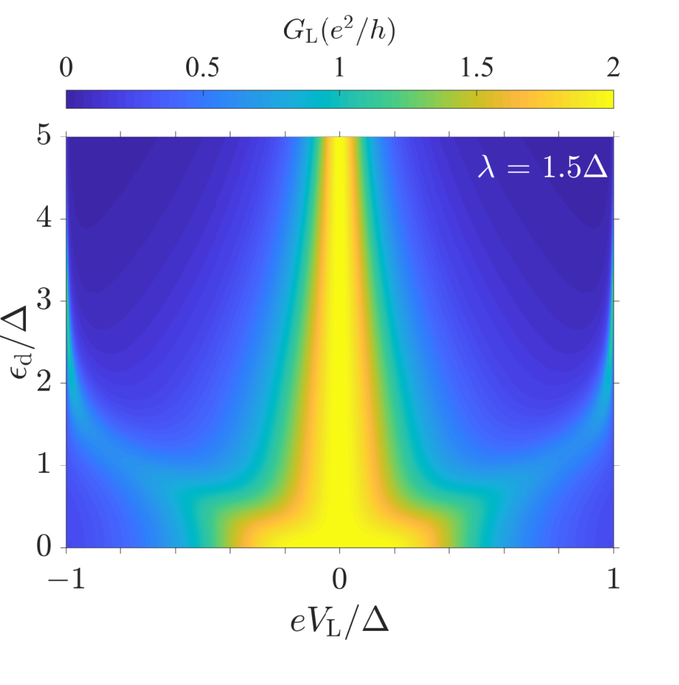
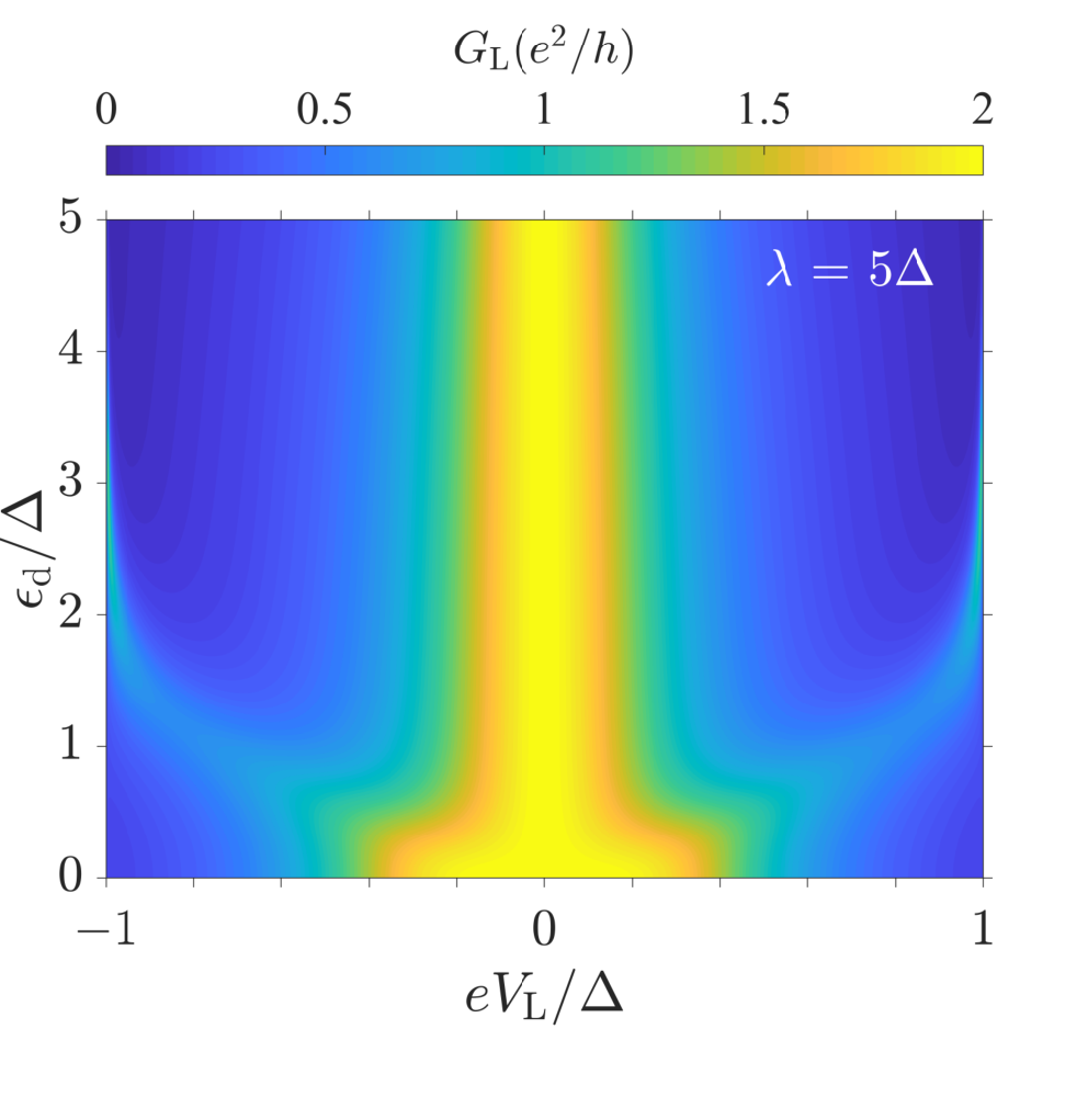
Figure 2: (a)-(c) Differential conductance spectra of the normal-metal lead as functions of e​VL/ΔeV_{\mathrm{L}}/\Delta and ϵd/Δ\epsilon_{\mathrm{d}}/\Delta at zero temperature. The parameters are ΓL=ΓR=0.8​Δ\Gamma_{\mathrm{L}}=\Gamma_{\mathrm{R}}=0.8\Delta, tmin=0.001​Δt_{\min}=0.001\Delta, and tmax=Δt_{\max}=\Delta. (e)-(f) The LDOS of the superconducting lead with the same parameters in (a)-(c). The LDOS is defined by the sum of the diagonal spectral function of the superconducting lead, i.e., ρ(ω)=−Im[TrGRR]/π\rho(\omega)=-\mathrm{Im}\left[\mathrm{Tr}\thinspace G_{\mathrm{R}}^{R}\right]/\pi.

The differential conductances of the leads η\eta at zero temperature are obtained by Gη=d​Iη/d​VLG_{\eta}=dI_{\eta}/dV_{\mathrm{L}}. Especially, the ZBCPs at zero temperature are

lime​VL→0GL​(e​VL)\displaystyle\lim_{eV_{\mathrm{L}}\to 0}G_{\mathrm{L}}(eV_{\mathrm{L}}) ={2​e2h,λ≠0,e2h​16​ΓL2​ΓR2(ΓL2+ΓR2+4​ϵd2)2,λ=0,\displaystyle=\begin{cases}\frac{2e^{2}}{h},&\lambda\neq 0,\\ \frac{e^{2}}{h}\frac{16\Gamma_{\mathrm{L}}^{2}\Gamma_{\mathrm{R}}^{2}}{(\Gamma_{\mathrm{L}}^{2}+\Gamma_{\mathrm{R}}^{2}+4\epsilon_{\mathrm{d}}^{2})^{2}},&\lambda=0,\end{cases} (24)
lime​VL→0GR​(e​VL)\displaystyle\lim_{eV_{\mathrm{L}}\to 0}G_{\mathrm{R}}(eV_{\mathrm{L}}) ={−e2h​4​ΓR2ΓL2+ΓR2+4​ϵd2,λ≠0,−e2h​16​ΓL2​ΓR2(ΓL2+ΓR2+4​ϵd2)2,λ=0,\displaystyle=\begin{cases}-\frac{e^{2}}{h}\frac{4\Gamma_{\mathrm{R}}^{2}}{\Gamma_{\mathrm{L}}^{2}+\Gamma_{\mathrm{R}}^{2}+4\epsilon_{\mathrm{d}}^{2}},&\lambda\neq 0,\\ -\frac{e^{2}}{h}\frac{16\Gamma_{\mathrm{L}}^{2}\Gamma_{\mathrm{R}}^{2}}{(\Gamma_{\mathrm{L}}^{2}+\Gamma_{\mathrm{R}}^{2}+4\epsilon_{\mathrm{d}}^{2})^{2}},&\lambda=0,\end{cases} (25)
lime​VL→0GY​(e​VL).\displaystyle\lim_{eV_{\mathrm{L}}\to 0}G_{\mathrm{Y}}(eV_{\mathrm{L}}). ={−e2h​2​(ΓL2−ΓR2+4​ϵd2)ΓL2+ΓR2+4​ϵd2,λ≠0,0,λ=0.\displaystyle=\begin{cases}-\frac{e^{2}}{h}\frac{2(\Gamma_{\mathrm{L}}^{2}-\Gamma_{\mathrm{R}}^{2}+4\epsilon_{\mathrm{d}}^{2})}{\Gamma_{\mathrm{L}}^{2}+\Gamma_{\mathrm{R}}^{2}+4\epsilon_{\mathrm{d}}^{2}},&\lambda\neq 0,\\ 0,&\lambda=0.\end{cases} (26)

When λ=0\lambda=0, the Majorana Y junction is disconnected with the QD, and the remaining part is reduced to an N-QD-S structure. The maximal ZBCP in Eq. (24) is equal to 4​e2/h4e^{2}/h when the QD is symmetrically coupled (ΓL=ΓR)(\Gamma_{\mathrm{L}}=\Gamma_{\mathrm{R}}) and on resonance (ϵd=0)(\epsilon_{\mathrm{d}}=0), in accord with the previous results of Ref. (Cao et al. 2004). When λ≠0\lambda\neq 0, the ZBCP of the normal-metal lead in this three-terminal structure equals a quantized value 2​e2/h2e^{2}/h, which is consistent with the famous conductance peak for the N-TS tunneling. As depicted in Figs. 2a-2c, the ZBCP is obviously broad for ϵd=0\epsilon_{\mathrm{d}}=0 and becomes sharp for large ϵd\epsilon_{\mathrm{d}}. The QD acts as a transfer station of electrons and holes, which means that the energy level of the QD is the tunnel barrier of the system. Hence the broadening of the ZBCP arises from the junction transparency effect and the height of the ZBCP is not affected. This quantized ZBCP is caused by the perfect Majorana-induced Andreev reflection. In the next section, we will show that the local Andreev reflection can be completely suppressed by increasing ϵd\epsilon_{\mathrm{d}}, and only the crossed Andreev reflection remains. We emphasize again that this ZBCP of 2​e2/h2e^{2}/h can completely arise from the crossed Andreev reflection, which is strongly protected by the superconducting gap Δ\Delta (Peng et al. 2015). Moreover, the results of Eqs. 25 and 26 show that the ZBCPs of both the superconducting and the Majorana leads are insensitive to the nonzero coupling amplitude λ\lambda, but only dependent on ΓL\Gamma_{\mathrm{L}}, ΓR\Gamma_{R} and ϵd\epsilon_{\mathrm{d}}.

The conductance peaks of the normal-metal lead are closely related to the local density of states (LDOS) of the superconducting lead in this T-shaped structure (the details of the analytical derivation of the LDOS are provided in Appendix B). As shown in Figs. 2d-2f, there are three subgap resonances in the superconducting lead two are the spin-induced resonances situating near the gap edge (Koerting et al. 2010), one is the Majorana-induced resonance situating at ω=0\omega=0. The conductance peaks are all situated at the subgap resonance energy. As ϵd\epsilon_{\mathrm{d}} increases, all the resonances become sharper, and the two near the gap edge merge with the dips eventually, whereas the one at ω=0\omega=0 remains. For large ϵd\epsilon_{\mathrm{d}}, the Majorana-induced resonance situating at ω=0\omega=0 sharpens to form a localized bound state, i.e., a Yu-Shiba-Rusinov state (YSR state). The occurrence of the Majorana-induced YSR state will lead to the domination of crossed Andreev reflection, which will be discussed in the next section. The Majorana-induced resonance in the superconducting lead is not quantized but parameters dependent, consistent with the result in Eq. 25. The Majorana-induced resonance leads to a quantized ZBCP of the normal-metal lead since the electrons and holes are transported through perfect Andreev reflection (Pan et al. 2021). The spin-induced conductance peaks are unstable and unquantized, i.e., they are not robust as functions of parameters. When λ\lambda increases, the Majorana induced resonance is enhanced and the spin-induced conductance peaks become inconspicuous in Figs. 2b and 2c due to the competition between the spin-induced and the Majorana-induced resonances in the tunneling processes.

Figure 3: ZBCP of the normal-metal lead as a function of finite temperature. The parameters are ΓL=ΓR=0.8​Δ\Gamma_{\mathrm{L}}=\Gamma_{\mathrm{R}}=0.8\Delta, λ=Δ\lambda=\Delta, tmin=10−3​Δt_{\min}=10^{-3}\Delta, and tmax=Δt_{\max}=\Delta.

The discussion can easily extend to finite temperature regimes. As shown in Fig. 3, the ZBCP of the normal-metal lead is no longer quantized to 2​e2/h2e^{2}/h, since the Fermi distribution is smoothly dependent on the temperature TT, which is called the thermal broadening. Nevertheless, we find that the effect of the thermal broadening is significantly suppressed by large junction transparency (ϵd=0CLOSE(\epsilon_{\mathrm{d}}=0). In Fig. 3, the ZBCP is pretty close to 2​e2/h2e^{2}/h when kB​T<Δ/20k_{B}T<\Delta/20. Such a temperature condition can be met in the experiment, e.g., see Ref. (Mourik et al. 2012), in which the induced superconducting gap of the InSb nanowires is Δ≈250​μ​eV\Delta\approx 250\mathrm{\mu eV} and the minimized temperature is kB​T≈4.3​μ​eVk_{B}T\approx 4.3\mathrm{\mu eV}.

IV SHOT NOISE AND FANO FACTOR

In addition to the time-average current, the shot noise can reveal the fluctuation of the current and provide useful information about MZMs (Bolech and Demler 2007; Nilsson et al. 2008; Golub and Horovitz 2011; Fu and Kane 2009b). The shot noise, defined as the correlation function of the current fluctuations between leads η\eta and η′\eta^{\prime}, takes the form Sη​η′​(t,t′)=⟨{δ​Iη​(t),δ​Iη′​(t′)}⟩S_{\eta\eta^{\prime}}(t,t^{\prime})=\left\langle\{\delta I_{\eta}(t),\delta I_{\eta^{\prime}}(t^{\prime})\}\right\rangle, where δ​Iη​(t)=I^η​(t)−Iη\delta I_{\eta}(t)=\hat{I}_{\eta}(t)-I_{\eta}, and I^η​(t)=−e​N˙η​(t)\hat{I}_{\eta}(t)=-e\dot{N}_{\eta}(t). The time-average current IηI_{\eta} has been obtained by Eq. (9). With the use of the Wick’s theorem and the S-matrix expansion (Souza et al. 2008; Wu and Cao 2012), we can reduce the expression of the shot noise in terms of Green’s functions. After Fourier transform, we obtain the expression of shot noise in the frequency space Sη​η′​(ω′)S_{\eta\eta^{\prime}}(\omega^{\prime}). The calculation of the shot noise is shown explicitly in Appendix C.

Following Ref.  (Blanter and Büttiker 2000), in multi-terminal systems, the shot noise Sη​η′​(ω′)S_{\eta\eta^{\prime}}(\omega^{\prime}) with η=η′\eta=\eta^{\prime} must be positive; conversely, that with η≠η′\eta\neq\eta^{\prime} must be negative. This property can be verified by the numerical calculation of Sη​η​(0)S_{\eta\eta}(0) in the following. The zero-frequency Fano factor, defined by the ratio Fη=Sη​η​(0)/2​e​IηF_{\eta}=S_{\eta\eta}(0)/2eI_{\eta}, can gain insight into the nature of charge quanta transferred to lead η\eta (Golub and Horovitz 2011; Cron et al. 2001; Cuevas et al. 1999). Beyond the linear regime in this paper, the Majorana-induced nonlinear effective charge has been studied in detail (Smirnov 2017), which gives rise to fractional effective charge quanta.

Figure 4: When the Majorana lead is disconnected to the QD (λ=0\lambda=0), electrons in the S lead are transferred to the N lead through conventional Andreev reflection; when the Majorana lead is connected to the QD (λ≠\lambda\neq0), the MZM γ2\gamma_{2} is the coherent superposition of electrons and holes with only spin ↑\uparrow, which leads to the first kind of crossed Andreev reflection. After braiding, the MZM γ3\gamma_{3} is coupled to the QD. Since γ3\gamma_{3} is the coherent superposition of electrons and holes with spins ↑\uparrow and ↓\downarrow, the second kind of crossed Andreev reflection occurs, which is equivalent to the splitting of charge quanta 3​e3e. We stress that both kinds of crossed Andreev reflection exist simultaneously after braiding.

The discussion will focus on the case of small transparency (ϵd≫ΔCLOSE(\epsilon_{\mathrm{d}}\gg\Delta) since we find that the Fano factors are quantized in this regime. In Fig. 5, we present the Fano factors at zero temperature as functions of ϵd/Δ\epsilon_{\mathrm{d}}/\Delta for a specific realization. In the case of λ=0\lambda=0, the remaining N-QD-S junction shows a doubled shot noise in Fano factors FL​(ϵd≫Δ)=−FR​(ϵd≫Δ)=2F_{\mathrm{L}}(\epsilon_{\mathrm{d}}\gg\Delta)=-F_{\mathrm{R}}(\epsilon_{\mathrm{d}}\gg\Delta)=2 due to the transport of Cooper pairs through conventional Andreev reflection (de Jong and Beenakker 1994). When the Majorana Y junction is connected to the QD with λ≠0\lambda\neq 0, we find FL​(ϵd≫Δ)=−FY​(ϵd≫Δ)=1F_{\mathrm{L}}(\epsilon_{\mathrm{d}}\gg\Delta)=-F_{\mathrm{Y}}(\epsilon_{\mathrm{d}}\gg\Delta)=1 and |FR​(ϵd≫Δ)|=2|F_{\mathrm{R}}(\epsilon_{\mathrm{d}}\gg\Delta)|=2. The results denote that the unit of charge transferred between the QD and the normal-metal lead is ee as well as the Majorana lead, while the unit of charge transferred between the QD and the superconducting lead is 2​e2e. This is the process of the first kind of crossed Andreev reflection. A hole from the left lead is reflected as an electron into the Majorana lead, while a Cooper pair from the superconducting lead is reflected as a hole into the Majorana lead and an electron into the normal-metal lead (Nilsson et al. 2008), as shown in Fig. 4. The holes transferred through crossed Andreev reflection act as facilitators to propel the splitting of Cooper pairs, and do not contribute to the transferred charge. In this regime, local Andreev reflection is fully suppressed, and the first kind of crossed Andreev reflection dominates.

The quantized Fano factors result from the occurrence of the YSR state below the gap. As shown in Fig. 2d, a very sharp Majorana-induced mid-gap resonance at ω=0\omega=0 when ϵd≫Δ\epsilon_{\mathrm{d}}\gg\Delta is regarded as a YSR bound state. The occurrence of the YSR state means that the Cooper pairing is “softened” so that the free electrons from the superconducting lead screen the spins of the QD (Heinrich et al. 2018; Maurand and Schönenberger 2013). The state-screened process leads to the splitting of Cooper pairs. In this way, crossed Andreev reflection dominates the tunneling processes, which gives rise to the quantized Fano factor.

Figure 5: Fano factors at zero temperature of the left lead (solid lines), right lead (dashed lines) and Majorana lead (dotted lines) as functions of ϵd\epsilon_{\mathrm{d}}. The parameters are e​VL=0.5​ΔeV_{\mathrm{L}}=0.5\Delta, ΓL=ΓR=0.8​Δ\Gamma_{\mathrm{L}}=\Gamma_{\mathrm{R}}=0.8\Delta, tmin=0.001​Δt_{\min}=0.001\Delta, and tmax=Δt_{\max}=\Delta.

V SIGNATURES OF THE MAJORANA BRAIDING

Now we braid the MZMs by taking γ2→−γ3\gamma_{2}\rightarrow-\gamma_{3} and γ3→γ2\gamma_{3}\rightarrow\gamma_{2}. Since the spin orientations of the MZMs γ2\gamma_{2} and γ3\gamma_{3} belonging to the same complex fermion c2c_{2} are different, observable consequences can be obtained with the connection to the QD. The QD is connected to the Majorana Y junction through γ3\gamma_{3}. Using the Nambu spinors and Eq. (5), we can easily obtain the Hamiltonian of the Majorana Y junction ℋ~Y\widetilde{\mathcal{H}}_{\mathrm{Y}} after braiding. Given that the angle of spin orientations between γ2\gamma_{2} and γ3\gamma_{3} is θ\theta, the spin-conserving coupling is then given by H~T,Y=−λ​d~↑​γ3+H.c.\widetilde{H}_{\mathrm{T,Y}}=-\lambda\widetilde{d}_{\uparrow}\gamma_{3}+\mathrm{H.c.}, where d~↑\widetilde{d}_{\uparrow} (d~↓)(\widetilde{d}_{\downarrow}) is the electron operators of the QD with the same (opposite) spin orientation described by γ3\gamma_{3} with

(d~↑d~↓)=(cos⁡θ2sin⁡θ2−sin⁡θ2cos⁡θ2)​(d↑d↓).\left(\begin{array}[]{c}\widetilde{d}_{\uparrow}\\ \widetilde{d}_{\downarrow}\end{array}\right)=\left(\begin{array}[]{cc}\cos\frac{\theta}{2}&\sin\frac{\theta}{2}\\ -\sin\frac{\theta}{2}&\cos\frac{\theta}{2}\end{array}\right)\left(\begin{array}[]{c}d_{\uparrow}\\ d_{\downarrow}\end{array}\right). (27)
Refer to caption
(a)
Refer to caption
(b)
Refer to caption
(c)
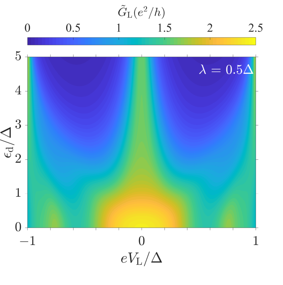
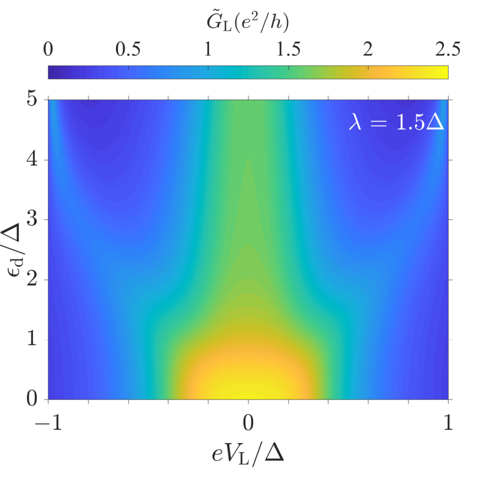
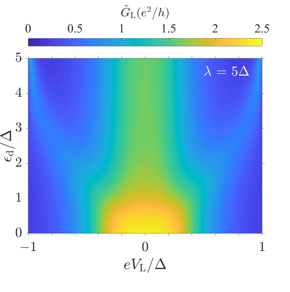
Figure 6: Differential conductance spectra of the normal-metal lead as a function of e​VL/ΔeV_{\mathrm{L}}/\Delta and ϵd/Δ\epsilon_{\mathrm{d}}/\Delta after braiding at zero temperature. The parameters are the same as in Fig. 2

For the Majorana Y junction sketched in Fig. 1, the spin orientation angle is θ=23​π\theta=\frac{2}{3}\pi. Such a braiding process is equivalent to involving spin-flip tunneling between the QD and Majorana lead. After braiding, we can obtain the ZBCPs by

lime​VL→0G~L​(e​VL)\displaystyle\lim_{eV_{\mathrm{L}}\to 0}\widetilde{G}_{\mathrm{L}}(eV_{\mathrm{L}}) ={e2h​8​ΓL2​((ΓL2+ΓR2+4​ϵd2)2+ΓR4+ΓL2​ΓR2)(4​ΓL2+ΓR2)​(ΓL2+ΓR2+4​ϵd2)2,λ≠0,e2h​16​ΓL2​ΓR2(ΓL2+ΓR2+ϵd2)2,λ=0,\displaystyle=\begin{cases}\frac{e^{2}}{h}\frac{8\Gamma_{\mathrm{L}}^{2}((\Gamma_{\mathrm{L}}^{2}+\Gamma_{\mathrm{R}}^{2}+4\epsilon_{\mathrm{d}}^{2})^{2}+\Gamma_{\mathrm{R}}^{4}+\Gamma_{\mathrm{L}}^{2}\Gamma_{\mathrm{R}}^{2})}{(4\Gamma_{\mathrm{L}}^{2}+\Gamma_{\mathrm{R}}^{2})(\Gamma_{\mathrm{L}}^{2}+\Gamma_{\mathrm{R}}^{2}+4\epsilon_{\mathrm{d}}^{2})^{2}},\,\lambda\neq 0,\\ \frac{e^{2}}{h}\frac{16\Gamma_{\mathrm{L}}^{2}\Gamma_{\mathrm{R}}^{2}}{(\Gamma_{\mathrm{L}}^{2}+\Gamma_{\mathrm{R}}^{2}+\epsilon_{\mathrm{d}}^{2})^{2}},\,\thinspace\thinspace\thinspace\thinspace\thinspace\thinspace\thinspace\thinspace\thinspace\thinspace\thinspace\thinspace\thinspace\thinspace\thinspace\thinspace\thinspace\thinspace\thinspace\thinspace\thinspace\thinspace\thinspace\thinspace\thinspace\thinspace\thinspace\thinspace\thinspace\thinspace\thinspace\lambda=0,\end{cases} (28)
lime​VL→0G~R​(e​VL)\displaystyle\lim_{eV_{\mathrm{L}}\to 0}\widetilde{G}_{\mathrm{R}}(eV_{\mathrm{L}}) ={−e2h​4​ΓL2​ΓR2​(5​ΓL2+5​ΓR2+12​ϵd2)(4ΓL2+ΓR2)(ΓL2+ΓR2+4ϵd2)2,λ≠0,−e2h​16​ΓL2​ΓR2(ΓL2+ΓR2+ϵd2)2,λ=0,\displaystyle=\begin{cases}-\frac{e^{2}}{h}\frac{4\Gamma_{\mathrm{L}}^{2}\Gamma_{\mathrm{R}}^{2}(5\Gamma_{\mathrm{L}}^{2}+5\Gamma_{\mathrm{R}}^{2}+12\epsilon_{\mathrm{d}}^{2})}{\text{(4$\Gamma_{\mathrm{L}}^{2}$+$\Gamma_{\mathrm{R}}^{2}$)($\Gamma_{\mathrm{L}}^{2}$+$\Gamma_{\mathrm{R}}^{2}$+4$\epsilon_{\mathrm{d}}^{2}$)}^{2}},&\lambda\neq 0,\\ -\frac{e^{2}}{h}\frac{16\Gamma_{\mathrm{L}}^{2}\Gamma_{\mathrm{R}}^{2}}{(\Gamma_{\mathrm{L}}^{2}+\Gamma_{\mathrm{R}}^{2}+\epsilon_{\mathrm{d}}^{2})^{2}},&\lambda=0,\end{cases} (29)
lime​VL→0G~Y​(e​VL)\displaystyle\lim_{eV_{\mathrm{L}}\to 0}\widetilde{G}_{\mathrm{Y}}(eV_{\mathrm{L}}) ={−e2h​4​ΓL2​(2​ΓL2−ΓR2+8​ϵd2)(4ΓL2+ΓR2)(ΓL2+ΓR2+4ϵd2)​,λ≠0​,0​,λ=0.\displaystyle=\begin{cases}-\frac{e^{2}}{h}\frac{4\Gamma_{\mathrm{L}}^{2}(2\Gamma_{\mathrm{L}}^{2}-\Gamma_{\mathrm{R}}^{2}+8\epsilon_{\mathrm{d}}^{2})}{\text{(4$\Gamma_{\mathrm{L}}^{2}$+$\Gamma_{\mathrm{R}}^{2}$)($\Gamma_{\mathrm{L}}^{2}$+$\Gamma_{\mathrm{R}}^{2}$+4$\epsilon_{\mathrm{d}}^{2}$)}}\text{,}&\lambda\neq 0\text{,}\\ 0\text{,}&\lambda=0.\end{cases} (30)

When λ=0\lambda=0, the result is the same as that before braiding; when λ≠0\lambda\neq 0, the occurrence of spin-flip tunneling shifts the ZBCP. We plot the differential conductance of the normal-metal lead after the Majorana braiding in Fig. 6 for comparison to Fig. 2. Particularly, if the QD is symmetrically coupled (ΓL=ΓR=Γ\Gamma_{\mathrm{L}}=\Gamma_{\mathrm{R}}=\Gamma) , the ZBCP of the normal-metal lead maximally shifts to 2.4​e2/h2.4e^{2}/h for ϵd=0\epsilon_{\mathrm{d}}=0 and 1.6​e2/h1.6e^{2}/h for ϵd≫Δ\epsilon_{\mathrm{d}}\gg\Delta, which can act a robust hint of Majorana braiding. With the increasing of ϵd\epsilon_{\mathrm{d}}, the ZBCP gets broadened and its height gets lower concurrently. As shown in Fig. 7., the thermal broadening effect can also be suppressed by taking ϵd=0\epsilon_{\mathrm{d}}=0 and each solid line is closed to the corresponding zero-temperature limit when kB​T<Δ/20k_{B}T<\Delta/20. Consequently, it is appropriate to observe the ZBCP with large junction transparency.

Figure 7: ZBCP of the normal-metal lead after braiding as a function of the finite temperature. The parameters are the same as in Fig. 3.

The Fano factors after braiding are also quantized, but 2<|F~R​(ϵd≫Δ)|<32<|\widetilde{F}_{\mathrm{R}}(\epsilon_{\mathrm{d}}\gg\Delta)|<3, i.e., the unit of charge transferred between the QD and the superconducting lead is larger than that of a Cooper pair, as shown Fig. 8. This result is induced by involving both spins ↑\uparrow and ↓\downarrow in the coupling between the QD and the MZM γ3\gamma_{3}. As illustrated in Fig. 4, the second kind of crossed Andreev reflection occurs after the Majorana braiding.

Specifically, a Cooper pair transferred between the QD and the superconducting lead is accompanied by an extra electron and a hole, which leads to the 3​e3e charge quanta. One electron of the 3​e3e charge quanta is reflected as an electron into the normal-metal lead, while the other two are reflected as holes into the Majorana lead. Such a process of charge transmission is equivalent to the splitting of the 3​e3e charge quanta.

Figure 8: Fano factors after braiding at zero temperature of the left lead (solid lines), right lead (dashed lines) and Majorana lead (dotted lines) as functions of ϵd\epsilon_{\mathrm{d}}. The parameters are the same as in Fig. 5.

Given that the electrons coupled to the MZM γ3\gamma_{3} are composed of spin-↑\uparrow and ↓\downarrow electrons with a certain weight depending on the angle θ\theta (see Eq. (27)), both kinds of crossed Andreev reflection exist simultaneously, which leads to 2<|F~R​(ϵd≫Δ)|<32<|\widetilde{F}_{\mathrm{R}}(\epsilon_{\mathrm{d}}\gg\Delta)|<3. As shown in Fig. 8, the second kind of crossed Andreev reflection gains the dominance of the tunneling processes (corresponding to |F~R​(ϵd≫Δ)|→3|\widetilde{F}_{\mathrm{R}}(\epsilon_{\mathrm{d}}\gg\Delta)|\rightarrow 3) with increasing λ\lambda. As for the Majorana lead, the acceptance of spin-↑\uparrow and ↓\downarrow electrons with a certain weight is equivalent to the acceptance of an electron with spin polarization angle θ\theta in each current pulse, which gives rise to |F~Y​(ϵd≫Δ)|=1|\widetilde{F}_{\mathrm{Y}}(\epsilon_{\mathrm{d}}\gg\Delta)|=1. The units of the charge transferred between the normal-metal lead and the QD for both kinds of crossed Andreev reflection are identical, so the Fano factor of the normal-metal lead stays at |F~L​(ϵd≫Δ)|=1|\widetilde{F}_{\mathrm{L}}(\epsilon_{\mathrm{d}}\gg\Delta)|=1, the same as that before braiding.

VI CONCLUSION

We have studied the ZBCPs and the Fano factors of the T-shaped structure. We have shown that the ZBCP of the normal-metal lead is always quantized to 2​e2/h2e^{2}/h at zero temperature before braiding, which is quite robust at finite temperature when the QD is on-resonance. This quantized conductance can entirely arise from the Majorana-induced crossed Andreev reflection, which is protected by the energy gap of the superconducting lead. After Majorana braiding, the quantized ZBCP shifts and becomes dependent on the line widths ΓL\Gamma_{\mathrm{L}}, ΓR\Gamma_{\mathrm{R}} and the QD level ϵd\epsilon_{\mathrm{d}}. This variation is owing to the introduction of spin-flip tunneling between the Majorana lead and the QD after braiding. By analyzing the quantized Fano factors, we have found that the crossed Andreev reflection dominates over the conventional Andreev reflection when ϵd≫Δ\epsilon_{\mathrm{d}}\gg\Delta. We have also found a novel kind of crossed Andreev reflection equivalent to the splitting of the 3​e3e charge quanta. The quantized ZBCPs and Fano factors induced by the nonlocal crossed Andreev reflection provide strong fingerprint for MZMs.

Appendix A CALCULATION OF ΣY<\Sigma_{\mathrm{Y}}^{<}

In this section, we present the details of the analytical calculation of the terms containing ΣY<\Sigma_{\mathrm{Y}}^{<} in Eq. 9 . The lesser self-energy from the Majorana lead is given by

ΣY<=FY​(ΣYA−ΣYR)=−i​2​FY​Im​ΣYR,\Sigma_{\mathrm{Y}}^{<}=F_{\mathrm{Y}}(\Sigma_{\mathrm{Y}}^{A}-\Sigma_{\mathrm{Y}}^{R})=-i2F_{\mathrm{Y}}\mathrm{Im}\Sigma_{\mathrm{Y}}^{R}, (31)

where ΣYR\Sigma_{\mathrm{Y}}^{R} is determined by

κ\displaystyle\kappa ≈−8​λ2​tmax2−4​tmax2​ω++(ω+)3+2​λ2​(ω+)2−4​tmax2​ω++(ω+)3,\displaystyle\thickapprox\frac{-8\lambda^{2}t_{\max}^{2}}{-4t_{\mathrm{\max}}^{2}\omega^{+}+(\omega^{+})^{3}}+\frac{2\lambda^{2}(\omega^{+})^{2}}{-4t_{\mathrm{\max}}^{2}\omega^{+}+(\omega^{+})^{3}}, (32)

with ω+=ω+i​0+\omega^{+}=\omega+i0^{+}, as we mentioned in the main text (κ\kappa here is same to that appeared in Eq. (III)). We use the notation κ1\kappa_{1}and κ2\kappa_{2} to denote the first term and the second term of κ\kappa, respectively. Neglecting the high-order terms of (i​0+)n≥2(i0^{+})^{n\geq 2}, we can obtain the following expressions:

κ1\displaystyle\kappa_{1} =−8​λ2​tmax2(−4​tmax2​ω+ω3)−(4​tmax2−3​ω2)​(i​0+),\displaystyle=\frac{-8\lambda^{2}t_{\max}^{2}}{(-4t_{\mathrm{\max}}^{2}\omega+\omega^{3})-(4t_{\mathrm{\max}}^{2}-3\omega^{2})(i0^{+})}, (33)
κ2\displaystyle\kappa_{2} =2​λ2​ω2ω⁡(−4​tmax2+ω2)+(4​tmax2+ω2)​(i​0+).\displaystyle=\frac{2\lambda^{2}\omega^{2}}{\omega(-4t_{\mathrm{\max}}^{2}+\omega^{2})+(4t_{\mathrm{\max}}^{2}+\omega^{2})(i0^{+})}. (34)

Using the formula

limη→0+1x±i​η=𝒫​1x∓i​π​δ​(x),\lim_{\eta\rightarrow 0^{+}}\frac{1}{x\pm i\eta}=\mathcal{P}\frac{1}{x}\mp i\pi\delta(x), (35)

we can obtain

i​Im​(κ1)\displaystyle i\mathrm{Im(\kappa_{1})} =i​π​−8​λ2​tmax24​tmax2−3​ω2​δ​(−4​tmax2​ω+ω34​tmax2−3​ω2),\displaystyle=i\pi\frac{-8\lambda^{2}t_{\max}^{2}}{4t_{\max}^{2}-3\omega^{2}}\delta\left(\frac{-4t_{\max}^{2}\omega+\omega^{3}}{4t_{\max}^{2}-3\omega^{2}}\right), (36)
i​Im​(κ2)\displaystyle i\mathrm{Im}(\kappa_{2}) =−i​π​2​λ2​ω24​tmax2+ω2​δ​(−4​tmax2​ω+ω34​tmax2+ω2).\displaystyle=-i\pi\frac{2\lambda^{2}\omega^{2}}{4t_{\max}^{2}+\omega^{2}}\delta\left(\frac{-4t_{\max}^{2}\omega+\omega^{3}}{4t_{\max}^{2}+\omega^{2}}\right). (37)

Using the relationship

δ⁡(ϕ⁡(x))=∑j1|ϕ′​(x)|​δ​(x−xj),\delta(\phi(x))=\sum_{j}\frac{1}{|\phi^{\prime}(x)|}\delta(x-x_{j}), (38)

with ϕ⁡(xj)=0\phi(x_{j})=0, the imaginary part of κ1\kappa_{1}and κ2\kappa_{2} reduce to

i​Im​(κ1)\displaystyle i\mathrm{Im(\kappa_{1})} =Q1​(ω)​[δ⁡(ω)+δ⁡(ω−2​tmax)+δ⁡(ω+2​tmax)],\displaystyle=Q_{1}(\omega)[\delta(\omega)+\delta(\omega-2t_{\max})+\delta(\omega+2t_{\max})], (39)
i​Im​(κ2)\displaystyle i\mathrm{Im(\kappa_{2})} =Q2​(ω)​[δ⁡(ω)+δ⁡(ω−2​tmax)+δ⁡(ω+2​tmax)],\displaystyle=Q_{2}(\omega)[\delta(\omega)+\delta(\omega-2t_{\max})+\delta(\omega+2t_{\max})], (40)

where

Q1​(ω)\displaystyle Q_{1}(\omega) =i​π​−8​λ2​tmax24​tmax2−3​ω2​|(4​tmax2−3​ω2)2−(4​tmax2−3​ω2)2−6​ω2​(4​tmax2−ω2)|,\displaystyle=i\pi\frac{-8\lambda^{2}t_{\max}^{2}}{4t_{\max}^{2}-3\omega^{2}}\left|\frac{(4t_{\max}^{2}-3\omega^{2})^{2}}{-(4t_{\max}^{2}-3\omega^{2})^{2}-6\omega^{2}(4t_{\max}^{2}-\omega^{2})}\right|, (41)
Q2​(ω)\displaystyle Q_{2}(\omega) =−i​π​2​λ2​ω24​tmax2+ω2​|(4​tmax2+ω2)2(−4​tmax2+3​ω2)​(4​tmax2+ω2)−2​ω2​(−4​tmax2+ω2)|.\displaystyle=-i\pi\frac{2\lambda^{2}\omega^{2}}{4t_{\max}^{2}+\omega^{2}}\left|\frac{(4t_{\max}^{2}+\omega^{2})^{2}}{(-4t_{\max}^{2}+3\omega^{2})(4t_{\max}^{2}+\omega^{2})-2\omega^{2}(-4t_{\max}^{2}+\omega^{2})}\right|. (42)

It is obvious that Q1​(0)=−2​i​π​λ2Q_{1}(0)=-2i\pi\lambda^{2}, Q1​(±2​tmax)=i​π​λ2Q_{1}(\pm 2t_{\max})=i\pi\lambda^{2}, Q2​(0)=0Q_{2}(0)=0 and Q2​(±2​tmax)=−i​π​λ2Q_{2}(\pm 2t_{\max})=-i\pi\lambda^{2}. Since the electron-hole symmetry gives GQDR​(−ω)=−[GQDR​(ω)]∗G_{\mathrm{QD}}^{R}(-\omega)=-\left[G_{\mathrm{QD}}^{R}(\omega)\right]^{*}, i.e., GQDR​(0)G_{\mathrm{QD}}^{R}(0) is a purely imaginary function. Note that the imaginary part of GQDR​(0)G_{\mathrm{QD}}^{R}(0) is tiny, we can obtain GQDR​(0)≈0G_{\mathrm{QD}}^{R}(0)\approx 0. For example, the terms containing ΣY<\Sigma_{\mathrm{Y}}^{<} in Eq. (9) are calculated by

∫d​ω​GQDR​(ω)​ΣY<​(ω)\displaystyle\int\mathrm{d}\omega G_{\mathrm{QD}}^{R}(\omega)\Sigma_{\mathrm{Y}}^{<}(\omega) ∝∫d​ω​GQDR​(ω)​[i​Im​(κ1+κ2)]\displaystyle\propto\int\mathrm{d}\omega G_{\mathrm{QD}}^{R}(\omega)[i\mathrm{Im}(\kappa_{1}+\kappa_{2})]
=−2​i​π​λ2​GQDR​(0)\displaystyle=-2i\pi\lambda^{2}G_{\mathrm{QD}}^{R}(0)
=0,\displaystyle=0, (43)

and

∫d​ω​GQDR​(ω)​ΣY<​(ω)​GQDA​(ω)​ΣηA​(ω)\displaystyle\int\mathrm{d}\omega G_{\mathrm{QD}}^{R}(\omega)\Sigma_{\mathrm{Y}}^{<}(\omega)G_{\mathrm{QD}}^{A}(\omega)\Sigma_{\mathrm{\eta}}^{A}(\omega)
=i​π​λ2​[GQDR​(0)​Λ​GQDA​(0)​ΣηA​(0)]\displaystyle=i\pi\lambda^{2}\left[G_{\mathrm{QD}}^{R}(0)\Lambda G_{\mathrm{QD}}^{A}(0)\Sigma_{\mathrm{\eta}}^{A}(0)\right]
=0.\displaystyle=0. (44)

Hence we can take ΣY<=0\Sigma_{\mathrm{Y}}^{<}=0 in the calculation of the time-average current and the shot noise.

Appendix B CALCULATION OF THE LDOS OF THE SUPERCONDUCTING LEAD

For convenience, the whole system is divided into two subsystems, one is "quantum dot + Majorana Y-junction+Normal-metal lead", the other is the superconducting lead. The Hamiltonian of the superconducting lead is given by Eq. (3) in the main text,

HR=∑k​σϵR,k​σaR,k​σ†aR,k​σ+∑k(ΔaR,k↑†aR,−k↓†+H.c.).H_{\mathrm{R}}=\sum_{k\sigma}\epsilon_{\mathrm{R},k\sigma}a_{\mathrm{R},k\sigma}^{\dagger}a_{\mathrm{R},k\sigma}+\sum_{k}(\Delta a_{\mathrm{R},k\uparrow}^{\dagger}a_{\mathrm{R},-k\downarrow}^{\dagger}+\mathrm{H.c.}).

In the Nambu space (aR,k↑†,aR,−k↓,aR,−k↓†,aR,k↑)(a_{\mathrm{R},k\uparrow}^{\dagger},a_{\mathrm{R},-k\downarrow},a_{\mathrm{R},-k\downarrow}^{\dagger},a_{\mathrm{R},k\uparrow}), the unperturbed Green’s function of the BCS superconductor evaluated at the origin (r=0r=0) is represented as

gRR​(ω)\displaystyle g_{\mathrm{R}}^{R}(\omega) =∫d3​k​ei​k⋅rω+2−ξk2−Δ2​(ω++ξkΔΔω+−ξkω++ξkΔΔω+−ξk)\displaystyle=\int\mathrm{d}^{3}k\frac{e^{ik\cdot r}}{\omega_{+}^{2}-\xi_{k}^{2}-\Delta^{2}}\left(\begin{array}[]{cccc}\omega_{+}+\xi_{k}&\Delta\\ \Delta&\omega_{+}-\xi_{k}\\ &&\omega_{+}+\xi_{k}&\Delta\\ &&\Delta&\omega_{+}-\xi_{k}\end{array}\right)
=−ρR∫dξk1(ξk−ω+2−Δ2)​(ξk+ω+2−Δ2)(ω++ξkΔΔω+−ξkω++ξk−Δ−Δω+−ξk),\displaystyle=-\rho_{R}\int\mathrm{d}\xi_{k}\frac{1}{\left(\xi_{k}-\sqrt{\omega_{+}^{2}-\Delta^{2}}\right)\left(\xi_{k}+\sqrt{\omega_{+}^{2}-\Delta^{2}}\right)}\left(\begin{array}[]{cccc}\omega_{+}+\xi_{k}&\Delta\\ \Delta&\omega_{+}-\xi_{k}\\ &&\omega_{+}+\xi_{k}&-\Delta\\ &&-\Delta&\omega_{+}-\xi_{k}\end{array}\right),

where ρR\rho_{R} is the density of states and ω+=ω+i​η\omega_{+}=\omega+i\eta with η=0+\eta=0^{+}. We reduce the expression above by taking

ω+2−Δ2=ω2+i​ω​η−Δ2≈ω2−Δ2+i​sgn​(ω)​η.\sqrt{\omega_{+}^{2}-\Delta^{2}}=\sqrt{\omega^{2}+i\omega\eta-\Delta^{2}}\approx\sqrt{\omega^{2}-\Delta^{2}}+i\mathrm{sgn}(\omega)\eta.

When |Δ|>|ω||\Delta|>|\omega|, the pole (imaginary part >0) is ξk=\xi_{k}=i​Δ2−ω2i\sqrt{\Delta^{2}-\omega{}^{2}}; when |Δ|<|ω||\Delta|<|\omega|, the pole (imag part >0) is ξk=i​η\xi_{k}=i\eta+s​g​n​(ω)​ω2−Δ2sgn(\omega)\sqrt{\omega{}^{2}-\Delta^{2}}. Using the theorem of residues, we obtain the unperturbed Green’s function of the BCS superconductor as

gRR​(ω)\displaystyle g_{\mathrm{R}}^{R}(\omega) =[−θ⁡(|Δ|−|ω|)​π​ρR​1Δ2−ω2−i​θ​(|ω|−|Δ|)​π​ρR​s​g​n​(ω)ω2−Δ2]​(ωΔΔωω−Δ−Δω)\displaystyle=\left[-\theta(|\Delta|-|\omega|)\pi\rho_{R}\frac{1}{\sqrt{\Delta^{2}-\omega{}^{2}}}-i\theta(|\omega|-|\Delta|)\pi\rho_{R}\frac{sgn(\omega)}{\sqrt{\omega{}^{2}-\Delta^{2}}}\right]\left(\begin{array}[]{cccc}\omega&\Delta\\ \Delta&\omega\\ &&\omega&-\Delta\\ &&-\Delta&\omega\end{array}\right)
=−i​π​ρR​β​(1ΔωΔω11−Δω−Δω1),\displaystyle=-i\pi\rho_{R}\beta\left(\begin{array}[]{cccc}1&\frac{\Delta}{\omega}\\ \frac{\Delta}{\omega}&1\\ &&1&-\frac{\Delta}{\omega}\\ &&-\frac{\Delta}{\omega}&1\end{array}\right),

where β⁡(ω)=θ⁡(|Δ|−|ω|)​ωi​Δ2−ω2+θ⁡(|ω|−|Δ|)​|ω|ω2−Δ2\beta(\omega)=\theta(|\Delta|-|\omega|)\frac{\omega}{i\sqrt{\Delta^{2}-\omega{}^{2}}}+\theta(|\omega|-|\Delta|)\frac{|\omega|}{\sqrt{\omega{}^{2}-\Delta^{2}}}. The spectral function of the superconducting lead is given by

AR​(ω)=i⁡(GRR​(ω)−GRA​(ω))=−2​Im​GRR​(ω)A_{\mathrm{R}}(\omega)=i(G_{\mathrm{R}}^{R}(\omega)-G_{\mathrm{R}}^{A}(\omega))=-2\mathrm{Im}G_{\mathrm{R}}^{R}(\omega)

with

GRR​(ω)=((gRR​(ω))−1−ΣQDR​(ω))−1.G_{\mathrm{R}}^{R}(\omega)=\left(\left(g_{\mathrm{R}}^{R}(\omega)\right)^{-1}-\Sigma_{\mathrm{QD}}^{R}(\omega)\right)^{-1}.

The self-energy at the origin (r=0r=0) can be calculated as

ΣQDR​(ω)\displaystyle\Sigma_{\mathrm{QD}}^{R}(\omega) =∑kℋT,R†​GQDR​(ω)​ℋT,R\displaystyle=\sum_{k}\mathcal{H}_{\mathrm{T,R}}^{\dagger}G_{\mathrm{QD}}^{R}(\omega)\mathcal{H}_{\mathrm{T,R}}
=∑k|νR,k|2​GQDR​(ω)\displaystyle=\sum_{k}|\nu_{\mathrm{R,k}}|^{2}G_{\mathrm{QD}}^{R}(\omega)
=2​π​ρR​|νR,r=0|2​GQDR​(ω)\displaystyle=2\pi\rho_{\mathrm{R}}|\nu_{\mathrm{R,r=0}}|^{2}G_{\mathrm{QD}}^{R}(\omega)
=ΓR​GQDR​(ω),\displaystyle=\Gamma_{\mathrm{R}}G_{\mathrm{QD}}^{R}(\omega),

where we have used Fourier transform |νR,r|2=12​π​∑kei​k​r​|νR,k|2|\nu_{\mathrm{R,r}}|^{2}=\frac{1}{2\pi}\sum_{k}e^{ikr}|\nu_{\mathrm{R,k}}|^{2}. The density of states ρR\rho_{\mathrm{R}} around the Fermi-surface is approximately regarded as a constant. The effective Green’s function of the QD in the subsystem "quantum dot + Majorana Y-junction+Normal-metal lead" is given by

GQDR​(ω)=((gQDR​(ω))−1−ΣLR​(ω)−ΣYR​(ω))−1.G_{\mathrm{QD}}^{R}(\omega)=\left(\left(g_{\mathrm{QD}}^{R}(\omega)\right)^{-1}-\Sigma_{\mathrm{L}}^{R}(\omega)-\Sigma_{\mathrm{Y}}^{R}(\omega)\right)^{-1}.

Hence the LDOS of the superconducting lead is

ρ⁡(ω)=Tr⁡[AR​(ω)]/2​π.\rho(\omega)=\mathrm{Tr}\left[A_{\mathrm{R}}(\omega)\right]/2\pi.

Appendix C CALCULATION OF THE SHOT NOISE Sη​η′​(ω′)S_{\eta\eta^{\prime}}(\omega^{\prime})

In this section,we review the formalism for the shot noise which will be used in the main text (Souza et al. 2008; Wu and Cao 2012). We consider the Hamiltonian of a multi-terminal systems with a noninteracting central QD

H=∑ηHη+HQD+HT,H=\sum_{\eta}H_{\eta}+H_{\mathrm{QD}}+H_{T}, (45)

where Hη=∑k​σϵη,k​σ​aη,k​σ†​aη,k​σH_{\mathrm{\eta}}=\sum_{k\sigma}\epsilon_{\mathrm{\eta},k\sigma}a_{\mathrm{\mathrm{\eta}},k\sigma}^{\dagger}a_{\mathrm{\mathrm{\eta}},k\sigma} and HQD=∑σϵd​dσ†​dσH_{\mathrm{QD}}=\sum_{\sigma}\epsilon_{\mathrm{d}}d_{\sigma}^{\dagger}d_{\sigma}.

The tunneling Hamiltonian is given by

HT=∑η​k​σ(tk​σ​aη,k​σ†​dσ+t∗​dσ†​aη,k​σ),H_{T}=\sum_{\eta k\sigma}(t_{k\sigma}a_{\mathrm{\mathrm{\eta}},k\sigma}^{\dagger}d_{\sigma}+t^{*}d_{\sigma}^{\dagger}a_{\mathrm{\mathrm{\eta}},k\sigma}), (46)

where tk​σt_{k\sigma} is the tunneling amplitude between the leads η\eta and the QD. The definition of the shot noise is given by

Sη​η′​(t,t′)\displaystyle S_{\eta\eta^{\prime}}(t,t^{\prime}) =ℏ​⟨{δ​I^η​(t),δ​I^η′​(t′)}⟩\displaystyle=\hbar\left\langle\{\delta\hat{I}_{\eta}(t),\delta\hat{I}_{\eta^{\prime}}(t^{\prime})\}\right\rangle
=ℏ​⟨{I^η​(t),I^η′​(t′)}⟩−2​ℏ​⟨Iη​(t)⟩​⟨Iη′​(t′)⟩\displaystyle=\hbar\Biggl\langle\{\hat{I}_{\eta}(t),\hat{I}_{\eta^{\prime}}(t^{\prime})\}\Biggr\rangle-2\hbar\Biggl\langle I_{\eta}(t)\Biggr\rangle\Biggl\langle I_{\eta^{\prime}}(t^{\prime})\Biggr\rangle
=−e2ℏ∑k​k′​σ​σ′{tk​σtk′​σ′⟨aη​k​σ†(t)dσ(t)aη′′​k′​σ†(t′)dσ′(t′)⟩\displaystyle=-\frac{e^{2}}{\hbar}\sum_{kk^{\prime}\sigma\sigma^{\prime}}\Biggl\{t_{k\sigma}t_{k^{\prime}\sigma^{\prime}}\Biggl\langle a_{\eta k\sigma}^{\dagger}(t)d_{\sigma}(t)a_{{}^{\prime}\eta^{\prime}k^{\prime}\sigma}^{\dagger}(t^{\prime})d_{\sigma^{\prime}}(t^{\prime})\Biggr\rangle
−tk​σ​tk′​σ′∗​⟨aη​k​σ†​(t)​dσ​(t)​dσ′†​(t′)​aη′​k′​σ′​(t′)⟩\displaystyle\thinspace\thinspace\thinspace\thinspace\thinspace\thinspace\thinspace\thinspace\thinspace\thinspace\thinspace\thinspace\thinspace\thinspace-t_{k\sigma}t_{k^{\prime}\sigma^{\prime}}^{*}\Biggl\langle a_{\eta k\sigma}^{\dagger}(t)d_{\sigma}(t)d_{\sigma^{\prime}}^{\dagger}(t^{\prime})a_{\eta^{\prime}k^{\prime}\sigma^{\prime}}(t^{\prime})\Biggr\rangle
−tk​σ∗​tk′​σ′​⟨dσ†​(t)​aη​k​σ​(t)​aη′​k′​σ′†​(t′)​dσ′​(t′)⟩\displaystyle\thinspace\thinspace\thinspace\thinspace\thinspace\thinspace\thinspace\thinspace\thinspace\thinspace\thinspace\thinspace\thinspace\thinspace-t_{k\sigma}^{*}t_{k^{\prime}\sigma^{\prime}}\Biggl\langle d_{\sigma}^{\dagger}(t)a_{\eta k\sigma}(t)a_{\eta^{\prime}k^{\prime}\sigma^{\prime}}^{\dagger}(t^{\prime})d_{\sigma^{\prime}}(t^{\prime})\Biggr\rangle
+tk​σ∗tk′​σ′∗⟨dσ†(t)aη​k​σ(t)dσ′†(t′)aη′​k′​σ′(t′)⟩}+H.C.−2ℏ⟨Iη(t)⟩⟨Iη′(t′)⟩.\displaystyle\thinspace\thinspace\thinspace\thinspace\thinspace\thinspace\thinspace\thinspace\thinspace\thinspace\thinspace\thinspace\thinspace\thinspace+t_{k\sigma}^{*}t_{k^{\prime}\sigma^{\prime}}^{*}\Biggl\langle d_{\sigma}^{\dagger}(t)a_{\eta k\sigma}(t)d_{\sigma^{\prime}}^{\dagger}(t^{\prime})a_{\eta^{\prime}k^{\prime}\sigma^{\prime}}(t^{\prime})\Biggr\rangle\Biggr\}+\mathrm{H.C.}-2\hbar\Biggl\langle I_{\eta}(t)\Biggr\rangle\Biggl\langle I_{\eta^{\prime}}(t^{\prime})\Biggr\rangle. (47)

Using the notation for four-type of the two-particle Green’s functions

G1(2)​(τ,τ′)\displaystyle G_{1}^{(2)}(\tau,\tau^{\prime}) =i2​⟨TC​aη​k​σ†​(τ)​dσ​(τ)​aη′​k′​σ′†​(τ′)​dσ′​(τ′)⟩,\displaystyle=i^{2}\Biggl\langle T_{C}a_{\eta k\sigma}^{\dagger}(\tau)d_{\sigma}(\tau)a_{\eta^{\prime}k^{\prime}\sigma^{\prime}}^{\dagger}(\tau^{\prime})d_{\sigma^{\prime}}(\tau^{\prime})\Biggr\rangle, (48)
G2(2)​(τ,τ′)\displaystyle G_{2}^{(2)}(\tau,\tau^{\prime}) =i2​⟨TC​aη​k​σ†​(τ)​dσ​(τ)​dσ′†​(τ′)​aη′​k′​σ′​(τ′)⟩,\displaystyle=i^{2}\Biggl\langle T_{C}a_{\eta k\sigma}^{\dagger}(\tau)d_{\sigma}(\tau)d_{\sigma^{\prime}}^{\dagger}(\tau^{\prime})a_{\eta^{\prime}k^{\prime}\sigma^{\prime}}(\tau^{\prime})\Biggr\rangle, (49)
G3(2)​(τ,τ′)\displaystyle G_{3}^{(2)}(\tau,\tau^{\prime}) =i2​⟨TC​dσ†​(τ)​aη​k​σ​(τ)​aη′​k′​σ′†​(τ′)​dσ′​(τ′)⟩,\displaystyle=i^{2}\Biggl\langle T_{C}d_{\sigma}^{\dagger}(\tau)a_{\eta k\sigma}(\tau)a_{\eta^{\prime}k^{\prime}\sigma^{\prime}}^{\dagger}(\tau^{\prime})d_{\sigma^{\prime}}(\tau^{\prime})\Biggr\rangle, (50)
G4(2)​(τ,τ′)\displaystyle G_{4}^{(2)}(\tau,\tau^{\prime}) =i2​⟨TC​dσ†​(τ)​aη​k​σ​(τ)​dσ′†​(τ′)​aη′​k′​σ′​(τ′)⟩,\displaystyle=i^{2}\Biggl\langle T_{C}d_{\sigma}^{\dagger}(\tau)a_{\eta k\sigma}(\tau)d_{\sigma^{\prime}}^{\dagger}(\tau^{\prime})a_{\eta^{\prime}k^{\prime}\sigma^{\prime}}(\tau^{\prime})\Biggr\rangle, (51)

the shot noise can be expressed as

Sη​η′​(t,t′)\displaystyle S_{\eta\eta^{\prime}}(t,t^{\prime}) =e2ℏ∑k​k′,σ​σ′{tk​σtk′​σ′G1(2)>(t,t′)−tk​σtk′​σ′∗G2(2)>(t,t′)\displaystyle=\frac{e^{2}}{\hbar}\sum_{kk^{\prime},\sigma\sigma^{\prime}}\Biggl\{t_{k\sigma}t_{k^{\prime}\sigma^{\prime}}G_{1}^{(2)>}(t,t^{\prime})-t_{k\sigma}t_{k^{\prime}\sigma^{\prime}}^{*}G_{2}^{(2)>}(t,t^{\prime})
−tk​σ∗tk′​σ′G3(2)>(t,t′)+tk​σ∗tk′​σ′∗G4(2)>(t,t′)}+H.C.−2ℏ⟨Iη(t)⟩⟨Iη′(t′)⟩,\displaystyle\thinspace\thinspace\thinspace\thinspace\thinspace\thinspace\thinspace\thinspace\thinspace\thinspace\thinspace\thinspace-t_{k\sigma}^{*}t_{k^{\prime}\sigma^{\prime}}G_{3}^{(2)>}(t,t^{\prime})+t_{k\sigma}^{*}t_{k^{\prime}\sigma^{\prime}}^{*}G_{4}^{(2)>}(t,t^{\prime})\Biggr\}+\mathrm{H.C.}-2\hbar\Biggl\langle I_{\eta}(t)\Biggr\rangle\Biggl\langle I_{\eta^{\prime}}(t^{\prime})\Biggr\rangle, (52)

where Gi(2)>​(t,t′)G_{i}^{(2)>}(t,t^{\prime}) can be obtained from Gi(2)​(τ,τ′)G_{i}^{(2)}(\tau,\tau^{\prime}) via analtyical continuation. The expression of Gi(2)​(τ,τ′)G_{i}^{(2)}(\tau,\tau^{\prime}) can be reduced by using the S-matrix expansion and Wick’s theorem, and more details can be found in Ref. (Souza et al. 2008). After the reduction ofGi(2)G_{i}^{(2)}, we can obtain,

G1(2)​(τ,τ′)\displaystyle G_{1}^{(2)}(\tau,\tau^{\prime}) =tk​σ∗​tk′​σ′∗​∫∫d​τ1​d​τ2​Gη,k​σ​σ​(τ1,τ)​Gη′,k′​σ′​σ′​(τ2,τ′)\displaystyle=t_{k\sigma}^{*}t_{k^{\prime}\sigma^{\prime}}^{*}\int\int\mathrm{d}\tau_{1}\mathrm{d}\tau_{2}G_{\eta,k\sigma\sigma}(\tau_{1},\tau)G_{\eta^{\prime},k^{\prime}\sigma^{\prime}\sigma^{\prime}}(\tau_{2},\tau^{\prime})
×[GQD,σ​σ​(τ,τ1)​GQD,σ′​σ′​(τ′,τ2)−GQD,σ​σ′​(τ,τ2)​GQD,σ′​σ​(τ′,τ1)],\displaystyle\thinspace\thinspace\thinspace\times\left[G_{\mathrm{QD},\sigma\sigma}(\tau,\tau_{1})G_{\mathrm{QD},\sigma^{\prime}\sigma^{\prime}}(\tau^{\prime},\tau_{2})-G_{\mathrm{QD},\sigma\sigma^{\prime}}(\tau,\tau_{2})G_{\mathrm{QD},\sigma^{\prime}\sigma}(\tau^{\prime},\tau_{1})\right], (53)
G2(2)​(τ,τ′)\displaystyle G_{2}^{(2)}(\tau,\tau^{\prime}) =−δk​k′​σ′​σ′​η​η′​Gη,k​σ′​σ​(τ′,τ)​GQD,σ​σ′​(τ,τ′)\displaystyle=-\delta_{kk^{\prime}\sigma^{\prime}\sigma^{\prime}\eta\eta^{\prime}}G_{\eta,k\sigma^{\prime}\sigma}(\tau^{\prime},\tau)G_{\mathrm{QD},\sigma\sigma^{\prime}}(\tau,\tau^{\prime})
+tk​σ∗tk′​σ′∫∫dτ1dτ2Gη,k​σ​σ(τ1,τ)Gη′,k′​σ′​σ′(τ′,τ2)\displaystyle\thinspace\thinspace\thinspace+t_{k\sigma}^{*}t_{k^{\prime}\sigma^{\prime}}\int\int\mathrm{d}\tau_{1}\mathrm{d}\tau_{2}G_{\eta,k\sigma\sigma}(\tau_{1},\tau)G_{\eta^{\prime},k^{\prime}\sigma^{\prime}\sigma^{\prime}}(\tau^{\prime},\tau_{2})
×[GQD,σ​σ​(τ,τ1)​GQD,σ′​σ′​(τ2,τ′)−GQD,σ​σ′​(τ,τ′)​GQD,σ′​σ​(τ2,τ1)],\displaystyle\thinspace\thinspace\thinspace\times\left[G_{\mathrm{QD},\sigma\sigma}(\tau,\tau_{1})G_{\mathrm{QD},\sigma^{\prime}\sigma^{\prime}}(\tau_{2},\tau^{\prime})-G_{\mathrm{QD},\sigma\sigma^{\prime}}(\tau,\tau^{\prime})G_{\mathrm{QD},\sigma^{\prime}\sigma}(\tau_{2},\tau_{1})\right], (54)
G3(2)​(τ,τ′)\displaystyle G_{3}^{(2)}(\tau,\tau^{\prime}) =[G2(2)​(τ,τ′)]∗,\displaystyle=\left[G_{2}^{(2)}(\tau,\tau^{\prime})\right]^{*}, (55)
G4(2)​(τ,τ′)\displaystyle G_{4}^{(2)}(\tau,\tau^{\prime}) =[G1(2)​(τ,τ′)]∗,\displaystyle=\left[G_{1}^{(2)}(\tau,\tau^{\prime})\right]^{*}, (56)

where Gη,k​σ​σ​(τ1,τ)=−i⁡⟨TC​aη​k​σ​(τ1)​aη​k​σ†​(τ)⟩G_{\eta,k\sigma\sigma}(\tau_{1},\tau)=-i\Biggl\langle T_{C}a_{\eta k\sigma}(\tau_{1})a_{\eta k\sigma}^{\dagger}(\tau)\Biggr\rangle and GQD,σ​σ′​(τ,τ2)=−i⁡⟨TC​dσ​(τ)​dσ′†​(τ2)⟩G_{\mathrm{QD},\sigma\sigma^{\prime}}(\tau,\tau_{2})=-i\Biggl\langle T_{C}d_{\sigma}(\tau)d_{\sigma^{\prime}}^{\dagger}(\tau_{2})\Biggr\rangle. The two-particle Green’s functions above can be decomposed into the connected and disconnected terms, i.e., Gi(2)​(τ,τ′)=Gi,disc(2)​(τ,τ′)+Gi,conn(2)​(τ,τ′)G_{i}^{(2)}(\tau,\tau^{\prime})=G_{i,\mathrm{disc}}^{(2)}(\tau,\tau^{\prime})+G_{i,\mathrm{conn}}^{(2)}(\tau,\tau^{\prime}). The disconnected terms are given by

G1,disc(2)​(τ,τ′)\displaystyle G_{1,\mathrm{disc}}^{(2)}(\tau,\tau^{\prime}) =tk​σ∗​tk′​σ′∗​∫d​τ1​GQD,σ​σ​(τ,τ1)​Gη,k​σ​σ​(τ1,τ+)​∫d​τ2​GQD,σ′​σ′​(τ′,τ2)​Gη′,k′​σ′​(τ2,τ′⁣+),\displaystyle=t_{k\sigma}^{*}t_{k^{\prime}\sigma^{\prime}}^{*}\int\mathrm{d}\tau_{1}G_{\mathrm{QD},\sigma\sigma}(\tau,\tau_{1})G_{\eta,k\sigma\sigma}(\tau_{1},\tau^{+})\int\mathrm{d}\tau_{2}G_{\mathrm{QD},\sigma^{\prime}\sigma^{\prime}}(\tau^{\prime},\tau_{2})G_{\eta^{\prime},k^{\prime}\sigma^{\prime}}(\tau_{2},\tau^{\prime+}), (57)
G2,disc(2)​(τ,τ′)\displaystyle G_{2,\mathrm{disc}}^{(2)}(\tau,\tau^{\prime}) =tk​σ∗​tk′​σ′​∫d​τ1​GQD,σ​σ​(τ,τ1)​Gη,k​σ​σ​(τ1,τ+)​∫d​τ2​Gη′,k′​σ′​σ′​(τ′,τ2)​GQD,σ′​σ′​(τ2,τ′⁣+),\displaystyle=t_{k\sigma}^{*}t_{k^{\prime}\sigma^{\prime}}\int\mathrm{d}\tau_{1}G_{\mathrm{QD},\sigma\sigma}(\tau,\tau_{1})G_{\eta,k\sigma\sigma}(\tau_{1},\tau^{+})\int\mathrm{d}\tau_{2}G_{\eta^{\prime},k^{\prime}\sigma^{\prime}\sigma^{\prime}}(\tau^{\prime},\tau_{2})G_{\mathrm{QD},\sigma^{\prime}\sigma^{\prime}}(\tau_{2},\tau^{\prime+}), (58)
G3,disc(2)​(τ,τ′)\displaystyle G_{3,\mathrm{disc}}^{(2)}(\tau,\tau^{\prime}) =[G2,disc(2)​(τ,τ′)]∗,\displaystyle=\left[G_{2,\mathrm{disc}}^{(2)}(\tau,\tau^{\prime})\right]^{*}, (59)
G4,disc(2)​(τ,τ′)\displaystyle G_{4,\mathrm{disc}}^{(2)}(\tau,\tau^{\prime}) =[G1,disc(2)(τ,τ′)].∗\displaystyle=\left[G_{1,\mathrm{disc}}^{(2)}(\tau,\tau^{\prime})\right].^{*} (60)

The analytic continuation rules give

G1,disc(2)>​(t,t′)\displaystyle G_{1,\mathrm{disc}}^{(2)>}(t,t^{\prime}) =tk​σ∗​tk′​σ′∗​Fη,k​σ​(t,t)​Fη′,k′​σ′​(t′,t′),\displaystyle=t_{k\sigma}^{*}t_{k^{\prime}\sigma^{\prime}}^{*}F_{\eta,k\sigma}(t,t)F_{\eta^{\prime},k^{\prime}\sigma^{\prime}}(t^{\prime},t^{\prime}), (61)
G2,disc(2)>​(t,t′)\displaystyle G_{2,\mathrm{disc}}^{(2)>}(t,t^{\prime}) =−tk​σ∗​tk′​σ′​Fη,k​σ​(t,t)​Fη′,k′​σ′∗​(t′,t′),\displaystyle=-t_{k\sigma}^{*}t_{k^{\prime}\sigma^{\prime}}F_{\eta,k\sigma}(t,t)F_{\eta^{\prime},k^{\prime}\sigma^{\prime}}^{*}(t^{\prime},t^{\prime}), (62)
G3,disc(2)>​(t,t′)\displaystyle G_{3,\mathrm{disc}}^{(2)>}(t,t^{\prime}) =−tk​σ​tk′​σ′∗​Fη,k​σ∗​(t,t)​Fη′,k′​σ′​(t′,t′),\displaystyle=-t_{k\sigma}t_{k^{\prime}\sigma^{\prime}}^{*}F_{\eta,k\sigma}^{*}(t,t)F_{\eta^{\prime},k^{\prime}\sigma^{\prime}}(t^{\prime},t^{\prime}), (63)
G4,disc(2)>​(t,t′)\displaystyle G_{4,\mathrm{disc}}^{(2)>}(t,t^{\prime}) =tk​σ​tk′​σ′​Fη,k​σ∗​(t,t)​Fη′,k′​σ′∗​(t′,t′),\displaystyle=t_{k\sigma}t_{k^{\prime}\sigma^{\prime}}F_{\eta,k\sigma}^{*}(t,t)F_{\eta^{\prime},k^{\prime}\sigma^{\prime}}^{*}(t^{\prime},t^{\prime}), (64)

where

Fη,k​σ​(t,t)=∫d​t1​GQD,σ​σR​(t,t1)​Gη,k​σ​σ<​(t1,t)+GQD,σ​σ<​(t,t1)​Gη,k​σ​σA​(t1,t).F_{\eta,k\sigma}(t,t)=\int\mathrm{d}t_{1}G_{\mathrm{QD},\sigma\sigma}^{R}(t,t_{1})G_{\eta,k\sigma\sigma}^{<}(t_{1},t)+G_{\mathrm{QD},\sigma\sigma}^{<}(t,t_{1})G_{\eta,k\sigma\sigma}^{A}(t_{1},t). (65)

The total contribution of the disconnected terms is

⟨{I^η​(t),I^η′​(t′)}⟩disc\displaystyle\Biggl\langle\{\hat{I}_{\eta}(t),\hat{I}_{\eta^{\prime}}(t^{\prime})\}\Biggr\rangle_{\mathrm{disc}} =e2ℏ2∑k​k′​σ​σ′{tk​σtk′​σ′G1,disc(2)>(t,t′)−tk​σtk′​σ′∗G2,disc(2)>(t,t′)\displaystyle=\frac{e^{2}}{\hbar^{2}}\sum_{kk^{\prime}\sigma\sigma^{\prime}}\Biggl\{t_{k\sigma}t_{k^{\prime}\sigma^{\prime}}G_{1,\mathrm{disc}}^{(2)>}(t,t^{\prime})-t_{k\sigma}t_{k^{\prime}\sigma^{\prime}}^{*}G_{2,\mathrm{disc}}^{(2)>}(t,t^{\prime})
−tk​σ∗tk′​σ′G3,disc(2)>(t,t′)+tk​σ∗tk′​σ′∗G4,disc(2)>(t,t′)}+H.C.\displaystyle\thinspace\thinspace\thinspace-t_{k\sigma}^{*}t_{k^{\prime}\sigma^{\prime}}G_{3,\mathrm{disc}}^{(2)>}(t,t^{\prime})+t_{k\sigma}^{*}t_{k^{\prime}\sigma^{\prime}}^{*}G_{4,\mathrm{disc}}^{(2)>}(t,t^{\prime})\Biggr\}+\mathrm{H.C.}
=2​e2ℏ2​∑k​k′​σ​σ′|tk​σ|2​|tk′​σ′|2​[Fη,k​σ​(t,t)+Fη,k​σ∗​(t,t)]​[Fη′,k′​σ′​(t′,t′)+Fη′,k′​σ′∗​(t′,t′)].\displaystyle=2\frac{e^{2}}{\hbar^{2}}\sum_{kk^{\prime}\sigma\sigma^{\prime}}|t_{k\sigma}|^{2}|t_{k^{\prime}\sigma^{\prime}}|^{2}\left[F_{\eta,k\sigma}(t,t)+F_{\eta,k\sigma}^{*}(t,t)\right]\left[F_{\eta^{\prime},k^{\prime}\sigma^{\prime}}(t^{\prime},t^{\prime})+F_{\eta^{\prime},k^{\prime}\sigma^{\prime}}^{*}(t^{\prime},t^{\prime})\right]. (66)

Note that Ση,k​σ​σ<=|tk​σ|2​Gη,k​σ​σ<​(t1,t)\Sigma_{\eta,k\sigma\sigma}^{<}=|t_{k\sigma}|^{2}G_{\eta,k\sigma\sigma}^{<}(t_{1},t), the time-average current can be written as

⟨I^η​(t)⟩=eℏ​∑k​σ∫d​t1​[GQD,σ​σR​(t,t1)​Ση,k​σ​σ<+GQD,σ​σ<​(t,t1)​Ση,k​σ​σA]+H.C.,\Biggl\langle\hat{I}_{\eta}(t)\Biggr\rangle=\frac{e}{\hbar}\sum_{k\sigma}\int\mathrm{d}t_{1}\left[G_{\mathrm{QD},\sigma\sigma}^{R}(t,t_{1})\Sigma_{\eta,k\sigma\sigma}^{<}+G_{\mathrm{QD},\sigma\sigma}^{<}(t,t_{1})\Sigma_{\eta,k\sigma\sigma}^{A}\right]+\mathrm{H.C.},

and hence,

⟨I^η​(t)⟩​⟨I^η′​(t′)⟩=2​e2ℏ2​∑k​k′​σ​σ′|tk​σ|2​|tk′​σ′|2​[Fη,k​σ​(t,t)+Fη,k​σ∗​(t,t)]​[Fη′,k′​σ′​(t′,t′)+Fη′,k′​σ′∗​(t′,t′)].\Biggl\langle\hat{I}_{\eta}(t)\Biggr\rangle\Biggl\langle\hat{I}_{\eta^{\prime}}(t^{\prime})\Biggr\rangle=2\frac{e^{2}}{\hbar^{2}}\sum_{kk^{\prime}\sigma\sigma^{\prime}}|t_{k\sigma}|^{2}|t_{k^{\prime}\sigma^{\prime}}|^{2}\left[F_{\eta,k\sigma}(t,t)+F_{\eta,k\sigma}^{*}(t,t)\right]\left[F_{\eta^{\prime},k^{\prime}\sigma^{\prime}}(t^{\prime},t^{\prime})+F_{\eta^{\prime},k^{\prime}\sigma^{\prime}}^{*}(t^{\prime},t^{\prime})\right]. (67)

Therefore, the disconnected part of the shot noise (C22) and (C23) are canceled out:

⟨{I^η​(t),I^η′​(t′)}⟩disc−2​⟨I^η​(t)⟩​⟨I^η′​(t′)⟩=0.\Biggl\langle\{\hat{I}_{\eta}(t),\hat{I}_{\eta^{\prime}}(t^{\prime})\}\Biggr\rangle_{\mathrm{disc}}-2\Biggl\langle\hat{I}_{\eta}(t)\Biggr\rangle\Biggl\langle\hat{I}_{\eta^{\prime}}(t^{\prime})\Biggr\rangle=0. (68)

As the result, the remained part in the shot noise is only expressed by the connected part by

Sη​η′​(t,t′)\displaystyle S_{\eta\eta^{\prime}}(t,t^{\prime}) =ℏ​⟨{I^η​(t),I^η′​(t′)}⟩conn\displaystyle=\hbar\Biggl\langle\{\hat{I}_{\eta}(t),\hat{I}_{\eta^{\prime}}(t^{\prime})\}\Biggr\rangle_{\mathrm{conn}}
=e2ℏ​∑k​k′,σ​σ′{tk​σ​tk′​σ′​G1,conn(2)>​(t,t′)−tk​σ​tk′​σ′∗​G2,conn(2)>​(t,t′)−tk​σ∗​tk′​σ′​G3,conn(2)>​(t,t′)+tk​σ∗​tk′​σ′∗​G4,conn(2)>​(t,t′)}+H.C.\displaystyle=\frac{e^{2}}{\hbar}\sum_{kk^{\prime},\sigma\sigma^{\prime}}\Biggl\{t_{k\sigma}t_{k^{\prime}\sigma^{\prime}}G_{1,\mathrm{\mathrm{conn}}}^{(2)>}(t,t^{\prime})-t_{k\sigma}t_{k^{\prime}\sigma^{\prime}}^{*}G_{2,\mathrm{\mathrm{conn}}}^{(2)>}(t,t^{\prime})-t_{k\sigma}^{*}t_{k^{\prime}\sigma^{\prime}}G_{3,\mathrm{\mathrm{conn}}}^{(2)>}(t,t^{\prime})+t_{k\sigma}^{*}t_{k^{\prime}\sigma^{\prime}}^{*}G_{4,\mathrm{conn}}^{(2)>}(t,t^{\prime})\Biggr\}+\mathrm{H.C.}
=e2ℏ​∑k,σ|tk​σ|2​δη,η′​[Gη,k​σ​σ​(t′,t)​GQD,σ​σ​(t,t′)+Gη,k​σ​σ​(t,t′)​GQD,σ​σ​(t′,t)]>\displaystyle=\frac{e^{2}}{\hbar}\sum_{k,\sigma}|t_{k\sigma}|^{2}\delta_{\eta,\eta^{\prime}}\left[G_{\eta,k\sigma\sigma}(t^{\prime},t)G_{\mathrm{QD},\sigma\sigma}(t,t^{\prime})+G_{\eta,k\sigma\sigma}(t,t^{\prime})G_{\mathrm{QD},\sigma\sigma}(t^{\prime},t)\right]^{>}
−e2ℏ∑k​k′,σ​σ′|tk​σ|2|tk′​σ′|2{[∫dt1GQD,σ′​σ(t′,t1)Gη,k​σ​σ(t1,t)∫dt2GQD,σ​σ′(t,t2)Gη′,k′​σ′​σ′(t2,t′)]>\displaystyle\thinspace\thinspace\thinspace-\frac{e^{2}}{\hbar}\sum_{kk^{\prime},\sigma\sigma^{\prime}}|t_{k\sigma}|^{2}|t_{k^{\prime}\sigma^{\prime}}|^{2}\Biggl\{\left[\int\mathrm{d}t_{1}G_{\mathrm{QD},\sigma^{\prime}\sigma}(t^{\prime},t_{1})G_{\eta,k\sigma\sigma}(t_{1},t)\int\mathrm{d}t_{2}G_{\mathrm{QD},\sigma\sigma^{\prime}}(t,t_{2})G_{\eta^{\prime},k^{\prime}\sigma^{\prime}\sigma^{\prime}}(t_{2},t^{\prime})\right]^{>}
−[GQD,σ′​σ​(t,t′)​∫∫d​t1​d​t2​Gη,k​σ​σ​(t1,t)​GQD,σ​σ′​(t2,t1)​Gη′,k′​σ′​σ′​(t′,t2)]>\displaystyle\thinspace\thinspace\thinspace-\left[G_{\mathrm{QD},\sigma^{\prime}\sigma}(t,t^{\prime})\int\int\mathrm{d}t_{1}\mathrm{d}t_{2}G_{\eta,k\sigma\sigma}(t_{1},t)G_{\mathrm{QD},\sigma\sigma^{\prime}}(t_{2},t_{1})G_{\eta^{\prime},k^{\prime}\sigma^{\prime}\sigma^{\prime}}(t^{\prime},t_{2})\right]^{>}
−[GQD,σ′​σ(t′,t)∫∫dt1dt2Gη,k​σ​σ(t,t1)GQD,σ​σ′(t1,t2,)Gη′,k′​σ′​σ′(t2,t′)]>\displaystyle\thinspace\thinspace\thinspace-\left[G_{\mathrm{QD},\sigma^{\prime}\sigma}(t^{\prime},t)\int\int\mathrm{d}t_{1}\mathrm{d}t_{2}G_{\eta,k\sigma\sigma}(t,t_{1})G_{\mathrm{QD},\sigma\sigma^{\prime}}(t_{1},t_{2},)G_{\eta^{\prime},k^{\prime}\sigma^{\prime}\sigma^{\prime}}(t_{2},t^{\prime})\right]^{>}
+[∫dt1GQD,σ′​σ(t1,t′)Gη,k​σ​σ(t,t1)∫dτ2GQD,σ​σ′(t2,t)Gη′,k′​σ′​σ′(t′,t2)]>}+H.C.\displaystyle\thinspace\thinspace\thinspace+\left[\int\mathrm{d}t_{1}G_{\mathrm{QD},\sigma^{\prime}\sigma}(t_{1},t^{\prime})G_{\eta,k\sigma\sigma}(t,t_{1})\int\mathrm{d}\tau_{2}G_{\mathrm{QD},\sigma\sigma^{\prime}}(t_{2},t)G_{\eta^{\prime},k^{\prime}\sigma^{\prime}\sigma^{\prime}}(t^{\prime},t_{2})\right]^{>}\Biggr\}+\mathrm{H.C.}
=e2ℏTr{δη,η′(Ση>(t′,t)σ~zGQD<(t,t′)σ~z+GQD>(t′,t)σ~zΣη<(t,t′)σ~z)\displaystyle=\frac{e^{2}}{\hbar}\textrm{Tr}\Biggl\{\delta_{\eta,\eta^{\prime}}(\Sigma_{\eta}^{>}(t^{\prime},t)\widetilde{\sigma}_{z}G_{\mathrm{QD}}^{<}(t,t^{\prime})\widetilde{\sigma}_{z}+G_{\mathrm{QD}}^{>}(t^{\prime},t)\widetilde{\sigma}_{z}\Sigma_{\eta}^{<}(t,t^{\prime})\widetilde{\sigma}_{z})
−[∫d​t1​GQD​(t′,t1)​Ση​(t1,t)]>​σ~z​[∫d​t2​GQD​(t,t2)​Ση′​(t2,t′)]<​σ~z\displaystyle\thinspace\thinspace\thinspace-[\int\mathrm{d}t_{1}G_{\mathrm{QD}}(t^{\prime},t_{1})\Sigma_{\eta}(t_{1},t)]^{>}\widetilde{\sigma}_{z}[\int\mathrm{d}t_{2}G_{\mathrm{QD}}(t,t_{2})\Sigma_{\eta^{\prime}}(t_{2},t^{\prime})]^{<}\widetilde{\sigma}_{z}
+[GQD(t,t′)]>σ~z[∫∫dt1dt2Ση(t1,t)GQD(t2,t1,)Ση′(t′,t2)]<σ~z\displaystyle\thinspace\thinspace\thinspace+[G_{\mathrm{QD}}(t,t^{\prime})]^{>}\widetilde{\sigma}_{z}[\int\int\mathrm{d}t_{1}\mathrm{d}t_{2}\Sigma_{\eta}(t_{1},t)G_{\mathrm{QD}}(t_{2},t_{1},)\Sigma_{\eta^{\prime}}(t^{\prime},t_{2})]^{<}\widetilde{\sigma}_{z}
+[∫∫dt1dt2Ση(t,t1)GQD(t1,t2,)Ση′(t2,t′)]>σ~z[GQD(t′,t)]<σ~z\displaystyle\thinspace\thinspace\thinspace+[\int\int\mathrm{d}t_{1}\mathrm{d}t_{2}\Sigma_{\eta}(t,t_{1})G_{\mathrm{QD}}(t_{1},t_{2},)\Sigma_{\eta^{\prime}}(t_{2},t^{\prime})]^{>}\widetilde{\sigma}_{z}[G_{\mathrm{QD}}(t^{\prime},t)]^{<}\widetilde{\sigma}_{z}
−[∫d​t1​GQD​(t1,t′)​Ση​(t,t1)]>​σ~z​[∫d​t2​GQD​(t2,t)​Ση′​(t′,t2)]<​σ~z,\displaystyle\thinspace\thinspace\thinspace-[\int\mathrm{d}t_{1}G_{\mathrm{QD}}(t_{1},t^{\prime})\Sigma_{\eta}(t,t_{1})]^{>}\widetilde{\sigma}_{z}[\int\mathrm{d}t_{2}G_{\mathrm{QD}}(t_{2},t)\Sigma_{\eta^{\prime}}(t^{\prime},t_{2})]^{<}\widetilde{\sigma}_{z}, (69)

where GQDG_{\mathrm{QD}} is the 4×4\times4 matrix form of the elements GQD,σ′​σG_{\mathrm{QD},\sigma^{\prime}\sigma} and Ση\Sigma_{\eta} is the 4×4\times4 matrix form of the elements Ση,σ​σ=∑k|tk​σ|2​Gη,k​σ​σ\Sigma_{\eta,\sigma\sigma}=\sum_{k}|t_{k\sigma}|^{2}G_{\eta,k\sigma\sigma}. The matrix σ~z=diag⁡(1,−1,1,−1)\widetilde{\sigma}_{z}=\mathrm{diag}(1,-1,1,-1) describes the different charge of electrons and holes. Finally, we apply the convolution property of Fourier transform ∫−∞∞d⁡(t−t′)​ei​ω′​(t−t′)​x​(t−t′)​y​(t′−t)=12​π​∫−∞∞d​ω​F​[x]​(ω)​F​[y]​(ω+ω′)\int_{-\infty}^{\infty}\mathrm{d}(t-t^{\prime})e^{i\omega^{\prime}(t-t^{\prime})}x(t-t^{\prime})y(t^{\prime}-t)=\frac{1}{2\pi}\int_{-\infty}^{\infty}\mathrm{d}\omega F[x](\omega)F[y](\omega+\omega^{\prime}) to the above shot noise and obtain

Sη​η′​(ω′)\displaystyle S_{\eta\eta^{\prime}}(\omega^{\prime}) =∫−∞∞d⁡(t−t′)​ei​ω′​(t−t′)​Sη​η′​(t−t′)\displaystyle=\int_{-\infty}^{\infty}\mathrm{d}(t-t^{\prime})e^{i\omega^{\prime}(t-t^{\prime})}S_{\eta\eta^{\prime}}(t-t^{\prime})
=e2h∫−∞∞dωTr{δη,η′(Ση>(ω)σ~zGQD<(ω+ω′)σ~z+GQD>(ω)σ~zΣη<(ω+ω′)σ~z)\displaystyle=\frac{e^{2}}{h}\int_{-\infty}^{\infty}\mathrm{d}\omega\textrm{Tr}\{\delta_{\eta,\eta^{\prime}}(\Sigma_{\eta}^{>}(\omega)\widetilde{\sigma}_{z}G_{\mathrm{QD}}^{<}(\omega+\omega^{\prime})\widetilde{\sigma}_{z}+G_{\mathrm{QD}}^{>}(\omega)\widetilde{\sigma}_{z}\Sigma_{\eta}^{<}(\omega+\omega^{\prime})\widetilde{\sigma}_{z})
−[GQD​(ω)​Ση′​(ω)]>​σ~z​[GQD​(ω+ω′)​Ση​(ω+ω′)]<​σ~z−[Ση​(ω)​GQD​(ω)]>​σ~z​[Ση′​(ω+ω′)​GQD​(ω+ω′)]<​σ~z\displaystyle\thinspace\thinspace-[G_{\mathrm{QD}}(\omega)\Sigma_{\eta^{\prime}}(\omega)]^{>}\widetilde{\sigma}_{z}[G_{\mathrm{QD}}(\omega+\omega^{\prime})\Sigma_{\eta}(\omega+\omega^{\prime})]^{<}\widetilde{\sigma}_{z}-[\Sigma_{\eta}(\omega)G_{\mathrm{QD}}(\omega)]^{>}\widetilde{\sigma}_{z}[\Sigma_{\eta^{\prime}}(\omega+\omega^{\prime})G_{\mathrm{QD}}(\omega+\omega^{\prime})]^{<}\widetilde{\sigma}_{z}
+GQD>(ω)σ~z[Ση′(ω+ω′)GQD(ω+ω′)Ση(ω+ω′)]<σ~z+[Ση(ω)GQD(ω)Ση′(ω)]>σ~zGQD<(ω+ω′)σ~z}.\displaystyle\thinspace\thinspace+G_{\mathrm{QD}}^{>}(\omega)\widetilde{\sigma}_{z}[\Sigma_{\eta^{\prime}}(\omega+\omega^{\prime})G_{\mathrm{QD}}(\omega+\omega^{\prime})\Sigma_{\eta}(\omega+\omega^{\prime})]^{<}\widetilde{\sigma}_{z}+[\Sigma_{\eta}(\omega)G_{\mathrm{QD}}(\omega)\Sigma_{\eta^{\prime}}(\omega)]^{>}\widetilde{\sigma}_{z}G_{\mathrm{QD}}^{<}(\omega+\omega^{\prime})\widetilde{\sigma}_{z}\}. (70)
Acknowledgements.
We would like to thank Ze-Min Huang, Zhongbo Yan and Seishi Enomoto for helpful discussions. This work is supported in part by the National Natural Science Foundation of China under Grants No. 11875327, the Fundamental Research Funds for the Central Universities, and the Sun Yat-Sen University Science Foundation.

References