The Complex-Step Derivative Approximation on Matrix Lie Groups

A matrix Lie group $\mathcal{G}$ is a Lie group that consists of the set of $m\times m$ invertible matrices, where the group operation is matrix multiplication [14, Ch. 10.2]. From the definition of a group, a matrix Lie group is closed under matrix multiplication. That is, given $\mbf{X},\mbf{Y}\in\mathcal{G}$, it follows that $\mbf{XY}\in\mathcal{G}$. A matrix Lie group is a closed subgroup of the general linear group defined by [15, Ch. 1.1]

which is also a matrix Lie group. The matrix Lie algebra of $\mathcal{G}$ is denoted $\mathfrak{g}$, and is defined as [15, Ch. 3.3],

It can be shown that the matrix Lie algebra defined by (1) is a valid Lie algebra [15, Ch. 3.1], and is a vector space closed under the operation of the Lie bracket $[\cdot,\cdot]$, which can be computed by $[\mbf{A},\mbf{B}]=\mbf{A}\mbf{B}-\mbf{B}\mbf{A}\in\mathfrak{g},$ for all $\mbf{A},\mbf{B}\in\mathfrak{g}.$ The wedge operator $(\cdot)^{\wedge}:\mathbb{R}^{n}\to\mathfrak{g}$ maps a column matrix to the matrix Lie algebra. The exponential map $\exp(\cdot):\mathfrak{g}\to\mathcal{G}$ maps an element of the matrix Lie algebra to the matrix Lie group, and is computed using the matrix exponential. The only matrix Lie group elements $\mbf{X}\in\mathcal{G}$ that are considered in this paper are those that can be written as

where ${{\boldsymbol{\xi}}\in\mathbb{R}^{n}}$. The “vee” operator ${(\cdot)^{\vee}:\mathfrak{g}\to\mathbb{R}^{n}}$ maps an element of the matrix Lie algebra to a column matrix. The logarithmic map $\ln(\cdot):\mathcal{G}\to\mathfrak{g}$ maps an element of the matrix Lie group to the matrix Lie algebra, and is computed by the matrix logarithm. A parameterization of the group $\mathcal{G}$ can be retrieved from $\mbf{X}$ via

when the matrix logarithm is well defined. The adjoint representation of $\mbf{X}$ is denoted $\mathrm{Ad}(\mbf{X})$, such that ${(\mathrm{Ad}(\mbf{X}){\boldsymbol{\zeta}})^{\wedge}=\mbf{X}{\boldsymbol{\zeta}}^{\wedge}\mbf{X}^{-1}},\;{\boldsymbol{\zeta}}\in\mathbb{R}^{n}$. This leads to the identity

The Baker-Campbell-Hausdorff (BCH) formula is the solution to

and the exact solution is an infinite sum [1, Ch. 7.1.5]. A first-order approximation to the BCH formula is

which is exact in the event that $[{\boldsymbol{\xi}}_{1}^{\wedge},{\boldsymbol{\xi}}_{2}^{\wedge}]=\mbf{0}$. Such an approximation is typically used when both ${\boldsymbol{\xi}}_{1}$ and ${\boldsymbol{\xi}}_{2}$ are assumed to be small. The details of the special Euclidean groups $SE(2)$, $SE(3)$, and the group of double direct isometries $SE_{2}(3)$ can be found in the appendix.

The Gauss-Newton algorithm is an optimization algorithm appropriate for nonlinear least-squares functions of the form

where $\mbf{W}\in\mathbb{R}^{q\times q}$ is a symmetric positive definite weight matrix and ${\mbf{e}:\mathbb{R}^{p}\to\mathbb{R}^{q}}$ is some error function. Employing Newton’s method directly on (2) requires the Hessian of $J(\mbf{x})$, which is potentially difficult to obtain. An alternate strategy is to substitute a first-order approximation of $\mbf{e}(\mbf{x})$ about some nominal ${\bar{\mbf{x}}}$, given by [1, Ch. 4.3]

into (2), thus yielding the Jacobian and a Hessian approximation of $J(\mbf{x})$,

The Gauss-Newton algorithm then proceeds identically to Newton’s method, where the nominal point is iterated by ${\bar{\mbf{x}}}_{\ell}={\bar{\mbf{x}}}_{\ell-1}+\delta\mbf{x}_{\ell-1}$. The step $\delta\mbf{x}_{\ell-1}$ is calculated as

Consider the complex-differentiable function ${f:\mathbb{C}\to\mathbb{C}}$ perturbed about the nominal point $\bar{x}$ by $jh$ where $\bar{x},h\in\mathbb{R}$ and $j=\sqrt{-1}$. A Taylor series expansion yields

If $f(\bar{x})$ is assumed to be real for all real $\bar{x}$, then, to first order, taking the imaginary portion of (3) yields [11]

This is valid as long as $f(\bar{x})\in\mathbb{R}$ for all $\bar{x}\in\mathbb{R}$, and that derivatives are evaluated at strictly real nominal points. From a practical standpoint, a user is often attempting to find derivatives of $f:\mathbb{R}\to\mathbb{R}$. Providing that this can be extended to $f:\mathbb{C}\to\mathbb{C}$ such that $f$ is complex-differentiable, then with a minor abuse of notation, this can construct a derivative approximation for $f(x)$ as written in [11, 10],

Since there are no subtractive cancellation errors, the complex-step derivative approximation can produce machine-precision approximations by reducing $h$ to an arbitrarily small step size.

Consider a complex-differentiable function ${f:\mathcal{G}\to\mathbb{C}}$ where ${\mathcal{G}\subset GL(m,\mathbb{C})}$, ${\mbf{X}({\boldsymbol{\epsilon}}^{R})={\bar{\mbf{X}}}\exp({\boldsymbol{\epsilon}}^{R^{\wedge}})}$ is parametrizable by a perturbation ${{\boldsymbol{\epsilon}}^{R}=[\epsilon_{1}^{R}\;\epsilon_{2}^{R}\ldots\epsilon_{n}^{R}]^{\mathsf{T}}\in\mathbb{C}^{n}}$ on the right, and ${\bar{\mbf{X}}}\in\mathbb{R}^{m\times m}$ is some nominal value of $\mbf{X}$. Consider perturbing $f(\mbf{X}({\boldsymbol{\epsilon}}^{R}))$ by ${\boldsymbol{\epsilon}}^{R}=\mbf{0}+jh\mbf{1}_{i}$, where $\mbf{1}_{i}$ is the $i^{\mathrm{th}}$ column of the appropriately-dimensioned identity matrix $\mbf{1}$. The composition $f(\mbf{X}({\boldsymbol{\epsilon}}^{R}))$ has essentially recast $f$ as $f:\mathbb{C}^{n}\to\mathbb{C}$, from which a Taylor series expansion yields [14, Ch. 11.3]

Since it is assumed that $f({\bar{\mbf{X}}})\in\mathbb{R}$, taking the imaginary component of (4) yields an approximation for the derivative

The right Jacobian $\partial f(\mbf{X}({\boldsymbol{\epsilon}}^{R}))/\partial{\boldsymbol{\epsilon}}^{R}$ can be obtained by individually computing the derivatives using (5) with ${i=1,2,\ldots,n}$. The left Jacobian can identically be obtained by instead parametrizing $\mbf{X}$ with $\mbf{X}({\boldsymbol{\epsilon}}^{L})=\exp({\boldsymbol{\epsilon}}^{L^{\wedge}}){\bar{\mbf{X}}}$. This leads to

Note that the superscripts on ${\boldsymbol{\epsilon}}^{R}$ and ${\boldsymbol{\epsilon}}^{L}$ are simply labels that correspond to right and left perturbations, respectively, as opposed to exponents.

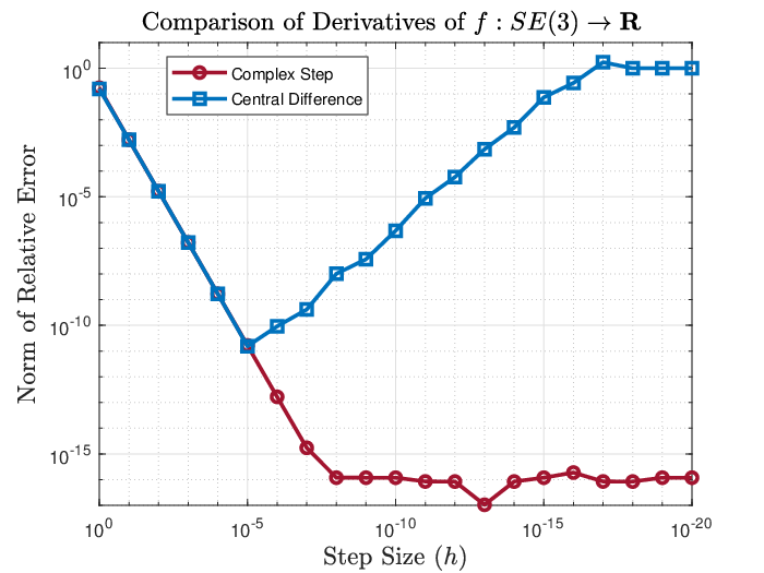
Example 1: Consider the function

where $\mbf{T}\in SE(3)$ and $\mbf{v},\mbf{y}\in\mathbb{R}^{4}$. The left Jacobian can be determined analytically using the first-order approximation $\mbf{T}=\exp({\boldsymbol{\epsilon}}^{L^{\wedge}}){\bar{\mbf{T}}}\approx(\mbf{1}+{\boldsymbol{\epsilon}}^{L^{\wedge}}){\bar{\mbf{T}}}$ and a Taylor series expansion. To this end,

where the $(\cdot)^{\odot}$ operator is defined in the appendix. The elements of $\partial f(\mbf{T}({\boldsymbol{\epsilon}}^{L}))/\partial{\boldsymbol{\epsilon}}^{L}$ are computed using (6) with varying step sizes $h$, and the results are compared with a central-difference scheme in Fig. 1. The error is computed by taking the relative 2-norm of the difference between the analytical and numerical solutions. Like the standard complex-step derivative, the complex-step derivative tailored to the matrix Lie group $SE(3)$ is able to achieve analytic accuracy, up to machine precision, for small enough $h$, while the central-difference derivative is not.

Example 2: Consider the nonlinear least-squares function

where $\mbf{T}=\exp({\boldsymbol{\epsilon}}^{L^{\wedge}}){\bar{\mbf{T}}}\in SE(3)$, $\mbf{W}\in\mathbb{R}^{6\times 6}$ is a symmetric positive definite weight matrix, and the error is given by

The matrix $\mbf{T}^{\mathrm{ref}}\in SE(3)$ is some reference point used to construct the error. The Jacobian $\partial\mbf{e}(\mbf{T}({\boldsymbol{\epsilon}}^{L}))/\partial{\boldsymbol{\epsilon}}^{L}$ can be used to construct Jacobian and Hessian approximations of $J(\mbf{x})$, which are used in the Gauss-Newton algorithm. Like in Example 1, the analytical left Jacobian can be determined by perturbing $\mbf{T}$ on the left,

where, in the last line, a first-order approximation to the BCH formula has been used.

The elements of the Jacobian $\partial\mbf{e}(\mbf{T}({\boldsymbol{\epsilon}}^{L}))/\partial{\boldsymbol{\epsilon}}^{L}$ were also calculated using (6) with a step size of $h=10^{-20}$. An optimization was performed with both Jacobian calculation methods, where the Gauss-Newton step $\delta{\boldsymbol{\epsilon}}_{\ell-1}$ is is determined from

and the argument of $\mbf{e}(\mbf{T}({\boldsymbol{\epsilon}}^{L}))$ is dropped for conciseness. The point is updated by

As shown in Fig. 2 using both an analytic Jacobian or a complex-step Jacobian results in an optimum being reached in a single step. Note that calculating Jacobians using the complex-step is shown to have a minor improvement in cost function reduction as compared to the analytical method. The reason is that the analytical method uses a first-order BCH approximation, which is ultimately slightly less accurate than the machine-precision complex-step Jacobian calculations.

The MAP approach [1, Ch. 8.2.5] to estimate the states in a batch framework results in the minimization of the least-squares cost function shown in (8), where the errors to be minimized are

The error term $\mbf{e}_{u,0}$ represents an error between the known initial state $\check{\mbf{T}}_{0}$, with uncertainty, and the estimated initial state $\mbf{T}_{0}$. This term is computed as

The process error terms $\mbf{e}_{u,1},\dots,\mbf{e}_{u,K}$ are a function of a discrete-time process model of the form ${\mbf{T}_{k}=\mbf{F}(\mbf{T}_{k-1},\mbf{u}_{k-1},\mbf{w}_{k-1})}$ where $\mbf{u}_{k-1}$ and $\mbf{w}_{k-1}$ are the input and zero-mean process noise at time $t_{k-1}$, respectively. These error terms are calculated as

Finally, the terms $\mbf{e}_{y,0},\dots,\mbf{e}_{y,K}$ correspond to the errors between measurements, and a measurement model of the form $\mbf{y}_{k}=\mbf{g}(\mbf{T}_{k},{\boldsymbol{\nu}}_{k})$, where ${\boldsymbol{\nu}}_{k}$ is zero-mean measurement noise. Hence, the measurement errors are

Following the MAP formulation the weight in (8) is

where the matrix $\mbf{P}_{0}$ is a covariance matrix associated with the uncertainty in the initial state, $\check{\mbf{T}}_{0}$. The matrices $\mbf{Q}_{k}$ and $\mbf{R}_{k}$ are covariance matrices associated with the process and measurement noises, respectively.

The goal is to find $\mbf{T}_{0},\ldots,\mbf{T}_{K}$ that minimize the least-squares cost function given by (8). To use a Gauss-Newton algorithm, the right (or left) Jacobian $\partial\mbf{e}(\mbf{T}({\boldsymbol{\epsilon}}^{R}))/\partial{\boldsymbol{\epsilon}}^{R}$ is needed, where ${\boldsymbol{\epsilon}}^{R}=[{\boldsymbol{\epsilon}}_{0}^{R^{\mathsf{T}}}\ldots{\boldsymbol{\epsilon}}_{K}^{R^{\mathsf{T}}}]^{\mathsf{T}}$ is a matrix that consists of perturbations to the individual estimated states. Since the error $\mbf{e}(\mbf{T}_{0},\ldots,\mbf{T}_{K})$ is a function of $K$ different Lie group elements, it is worth mentioning a simple technique that allows a user to treat the same function as a function of a single matrix Lie group element, as shown next in Section IV-B. The Jacobians can then be computed using (5) or (6).

Consider a function ${f(\mbf{X}_{0},\ldots,\mbf{X}_{K})\in\mathbb{R}}$ where ${\mbf{X}_{0},\ldots,\mbf{X}_{K}\in\mathcal{G}}$. Let ${\mbf{X}_{i}={\bar{\mbf{X}}}_{i}\exp({\boldsymbol{\epsilon}}_{i}^{R^{\wedge}})}$. Define ${\mbf{X}\mathrel{\mathop{\smash{=}}\limits^{\hbox{\raisebox{2.1097pt}{\small$\scriptstyle\triangle$}}}}\mathrm{diag}(\mbf{X}_{0},\ldots,\mbf{X}_{K})}$, thus leading to

By defining ${\boldsymbol{\epsilon}}^{R}\mathrel{\mathop{\smash{=}}\limits^{\hbox{\raisebox{2.1097pt}{\small$\scriptstyle\triangle$}}}}\left[{\boldsymbol{\epsilon}}_{0}^{R^{\mathsf{T}}}\ldots{\boldsymbol{\epsilon}}_{K}^{R^{\mathsf{T}}}\right]^{\mathsf{T}}$, ${\bar{\mbf{X}}}\mathrel{\mathop{\smash{=}}\limits^{\hbox{\raisebox{2.1097pt}{\small$\scriptstyle\triangle$}}}}\mathrm{diag}({\bar{\mbf{X}}}_{0},\ldots,{\bar{\mbf{X}}}_{K})$ along with a new operator $(\cdot)^{\triangle}$ such that ${{\boldsymbol{\epsilon}}^{\triangle}\mathrel{\mathop{\smash{=}}\limits^{\hbox{\raisebox{2.1097pt}{\small$\scriptstyle\triangle$}}}}\mathrm{diag}({\boldsymbol{\epsilon}}_{0}^{\wedge},\ldots,{\boldsymbol{\epsilon}}_{K}^{\wedge})}$, equation (IV-B) becomes

Therefore, a collection of matrix Lie group elements can be packaged into a single element of a new group. This can be done similarly with left perturbations.

The EuRoC micro aerial vehicle dataset collected by the Autonomous Systems Laboratory at ETH Zürich, Switzerland [12] includes accelerometer and gyroscope measurements, as well as ground truth position data. To simulate position measurements akin to GPS or UWB measurements, normally distributed random noise is added to the provided ground position data. The state of the rigid body can be represented by the matrix Lie group element ${\mbf{T}_{k}\in SE_{2}(3)}$, and as such the velocity is also estimated. The accelerometer measurements $\mbf{u}^{\mathrm{acc}}_{k}$ and gyroscope measurements $\mbf{u}^{\mathrm{gyro}}_{k}$ are treated as process-model inputs ${\mbf{u}_{k}=[\mbf{u}^{\mathrm{acc}^{\mathsf{T}}}_{k}\;\mbf{u}^{\mathrm{gyro}^{\mathsf{T}}}_{k}]^{\mathsf{T}}}$, while the position measurements $\mbf{y}^{\mathrm{pos}}_{k}$ are treated as measurement-model outputs.

For this problem, the analytical expression for the Jacobian $\partial\mbf{e}(\mbf{T})/\partial{\boldsymbol{\epsilon}}^{R}$ can be obtained, and the details of the derivation can be found in [16, Ch. 5]. Henceforth, the arguments of functions of multiple matrix Lie group elements will be consolidated under $\mbf{T}$, as described in Section IV-B. The right Jacobian is

where

where $T=t_{k}-t_{k-1}$, $\mbf{p}=[\mbf{0}\;1]^{\mathsf{T}}$, and $\mbf{g}$ is the gravity vector resolved in the datum frame. These expressions require first-order approximations to the BCH formula, similar to Example 2. This is common procedure, as the approximation becomes more accurate as errors become small [16, 1].

A Gauss-Newton optimization is performed on the MH_03_medium dataset. For simplicity, the accelerometer and gyroscope measurements are downsampled from the original 200 Hz in order to reduce the amount of variables in the optimization procedure. An alternative to downsampling is to perform IMU preintegration as described in [17], but this is beyond the scope of this paper. The specifications of the batch-estimation problem are shown in Table I. The process covariance matrix was set to,

Figure 3 shows a visualization of the trajectory once the optimization procedure has converged. Figure 4 shows the value of the cost function $J(\mbf{T})$ across the iterations of the Gauss-Newton algorithm. Since the initial guess for the states is obtained by dead reckoning, this sets all the process errors $\mbf{e}_{u,1},\ldots,\mbf{e}_{u,K}$ to zero. The first iteration attempts to decrease the measurement errors, resulting in an increase in process errors, and hence an increase in the overall cost function.

In this example, BCH approximations in the analytical Jacobians did not create any difference in the convergence history since the errors are initialized to be small in the the dead reckoning step. A central-difference scheme was also used to calculate Jacobians, and after multiple trial-and-error attempts with different step sizes, an identical convergence history to what is shown in Fig. 4 was obtained. However, the central-difference method requires twice as many function evaluations as the complex-step method, and therefore required approximately twice the total computing time. Finally, Fig. 5 shows the 2-norm of the difference between the batch-estimation solution and the ground truth. The errors are small, indicating the MAP framework has converged close to the ground truth.

The ‘Lost in the Woods’ dataset consists of a mobile wheeled robot navigating through a “forest” of tubes [13], as seen in Figure 6. The robot is equipped with wheel odometry providing forward velocity measurements, denoted $u^{\mathrm{vel}}_{k}$, and angular velocity measurements, denoted $u^{\mathrm{ang}}_{k}$. Furthermore, the robot has a laser range finder that provides range and bearing measurements to pre-identified landmarks (the tubes shown in Figure 6), denoted $r^{\ell}_{k},\phi^{\ell}_{k}$ for landmark $\ell$ at $t_{k}$, respectively. The positions of the landmarks in a datum reference frame are known in advance, and are denoted $\mbf{r}^{\ell}$. The state of the robot can be represented by $\mbf{T}_{k}\in SE(2)$.

The process model consists of the nonholonomic vehicle kinematics. Written in the form ${\mbf{T}_{k}=\mbf{F}(\mbf{T}_{k-1},\mbf{u}_{k-1},\mbf{w}_{k-1})}$,

where

$T=t_{k}-t_{k-1}$, and $w^{\mathrm{vel}}_{k-1},w^{\mathrm{ang}}_{k-1}$ are zero-mean normally distributed noises associated with the velocity and angular velocity measurements, respectively. The measurement model consists of the range and bearing measurements for each landmark. Written as $\mbf{y}=\mbf{g}(\mbf{T}_{k},{\boldsymbol{\nu}}_{k})$, the measurement model is

where ${\boldsymbol{\nu}}_{k}$ is zero-mean normally distributed measurement noise, $\mbf{D}=[\mbf{1}\;\mbf{0}]$, $\mbf{p}=[d\;0\;1]^{\mathsf{T}}$, and $d$ is the distance between the laser range finder and the reference point on the robot.

Computing the Jacobians associated with the measurement model by hand is, although not impossible, laborious due to the $\mathrm{atan2(\cdot,\cdot)}$ term. Hence, the complex-step derivative is used to directly evaluate the right Jacobian $\partial\mbf{e}(\mbf{T})/\partial{\boldsymbol{\epsilon}}^{R}$ for use in the Gauss-Newton optimization.

Dead reckoning was performed using wheel odometry in order to generate an initial guess for the Gauss-Newton optimization. All measurements were downsampled from the original 10 Hz to 5 Hz in order to limit the number of variables in the optimization procedure. The $\mbf{Q}_{k}$ and $\mbf{R}_{k}$ matrices were directly formed from the discrete-time covariances provided in the dataset [13]. The initial state $\mbf{T}_{0}$ was set to be a random perturbation from the ground truth.

The algorithm converged in 6 iterations, and produced a trajectory visualizable in Figure 7. The errors are shown in Figure 8, which show good performance when compared to the ground truth position and attitude data. This can also be achieved with central-difference, but again, the computation time is significantly longer, and the step sized must be tuned.

References

- [1] Tim Barfoot “State Estimation for Robotics” Toronto, ON: Cambridge University Press, 2019
- [2] P.A. Absil, R. Mahony and R. Sepulchre “Optimization Algorithms on Matrix Manifolds” Princeton Uni. Press, 2008
- [3] Nicolas Boumal, Bamdev Mishra, P.-A Absil and Rodolphe Sepulchre “Manopt, a Matlab Toolbox for Optimization on Manifolds” In Machine Learning Research 15, 2014, pp. 1455–1459
- [4] GTSAM “Math of GTSAM”, 2019, pp. 1–29 URL: https://github.com/borglab/gtsam
- [5] Klaus R“”obenack, Jan Winkler and Siqian Wang “LIEDRIVERS - A Toolbox for the Efficient Computation of Lie Derivatives Based on the Object-Oriented Algorithmic Differentiation Package ADOL-C” In Workshop on Equation-Based Object-Oriented Modeling Languages and Tools, 2011, pp. 57–66 ETH Zürich
- [6] Hannes Sommer, C“’edric Pradalier and Paul Furgale “Automatic Differentiation on Differentiable Manifolds as a Tool for Robotics” In Robotics Research: The 16th International Symposium, 2013, pp. 505–520
- [7] James Townsend and Sebastian Weichwald “Pymanopt: A Python Toolbox for Optimization on Manifolds using Automatic Differentiation” In Journal of Machine Learning Research 17.1, 2016, pp. 1–5
- [8] Hauke Strasdat “Sophus - Lie groups for 2D/3D Geometry”, 2019 URL: https://strasdat.github.io/Sophus/
- [9] Sameer Agarwal and Keir Mierle “Ceres Solver — A Large Scale Non-linear Optimization Library”, 2019 URL: http://ceres-solver.org/
- [10] Joaquim R R Martins, Peter Sturdza and Juan Alonso “The Complex-Step Derivative Approximation” In ACM Trans. on Mathematical Software 29.3, 2003, pp. 245–262
- [11] William Squire and George Trapp “Using Complex Variables to Estimate Derivatives of Real Functions” In SIAM Review 40.1, 1998, pp. 110–112
- [12] Michael Burri et al. “The EuRoC Micro Aerial Vehicle Datasets” In The International Journal of Robotics Research 35.10, 2016, pp. 1157–1163
- [13] Timothy Barfoot “AER 1513 Course Assignments” In State Estimation for Aerospace Vehicles Toronto, ON: Uni. of Toronto, 2009
- [14] Gregory. Chirikjian “Stochastic Models, Information Theory, and Lie Groups - Volume 2” Birkhäuser Boston, 2009
- [15] Brian Hall “Lie Groups, Lie Algebras and Representations” New York, NY: Springer, 2015
- [16] Jonathan Arsenault “Practical Considerations and Extensions of the Invariant Extended Kalman Filtering Framework”, 2019
- [17] Christian Forster, Luca Carlone, Frank Dellaert and Davide Scaramuzza “On-Manifold Preintegration for Real-Time Visual-Inertial Odometry” In IEEE Trans. Robotics 33.1, 2017, pp. 1–21
- [18] MDO Laboratory “A Guide to the Complex-Step Derivative Approximation” In University of Michigan, 2017 URL: http://mdolab.engin.umich.edu
- [19] Vivek Vittaldev, Ryan Russell, Nitin Arora and David Gaylor “Second-Order Kalman Filters Using Multi-Complex Step Derivatives” In Advances in the Astronautical Sciences 143.1, 2012, pp. 1–16
- [20] Valentin Peretroukhin and Jonathan Kelly “DPC-Net: Deep Pose Correction for Visual Localization” In IEEE Robotics and Automation Letters 3.3, 2018, pp. 2424–2431
- [21] K.-L Lai and J Crassidis “Extensions of the First and Second Complex-Step Derivative Approximations” In J. Comp. Applied Math 219.1, 2008, pp. 276–293