,
On sequences of records generated by planar random walks
Abstract
We investigate the statistics of three kinds of records associated with planar random walks, namely diagonal, simultaneous and radial records. The mean numbers of these records grow as universal power laws of time, with respective exponents 1/4, 1/3 and 1/2. The study of diagonal and simultaneous records relies on the underlying renewal structure of the successive hitting times and locations of translated copies of a fixed target. In this sense, this work represents a two-dimensional extension of the analysis made by Feller of ladder points, i.e., records for one-dimensional random walks. This approach yields a variety of analytical asymptotic results, including the full statistics of the numbers of diagonal and simultaneous records, the joint law of the epoch and location of the current diagonal record and the angular distribution of the current simultaneous record. The sequence of radial records cannot be constructed in terms of a renewal process. In spite of this, their mean number is shown to grow with a super-universal square-root law for isotropic random walks in any spatial dimension. Their full distribution is also obtained. Higher-dimensional diagonal and simultaneous records are also briefly discussed.
1 Introduction
An observation in a time series is called an (upper) record if it is larger than all previous observations in the series. The simplest case is when these observations are independent and identically distributed (iid) [1, 2, 3, 4, 5, 6, 7]. However, in many instances observations are not iid random variables. Consider for example the sequence of positions of a one-dimensional random walker. The points where the position reaches a record value, that is, where it exceeds all previously attained values, are called the ladder points, in the terminology of Feller [8, 9]. Ladder points are important because sections between them are probabilistic replicas of each other. This renewal structure makes the study of records for one-dimensional random walks amenable to exact analysis (see [9, chapters XII and XVIII]).
More recently, the statistics of records has found applications in a variety of complex physical systems such as disordered systems, aging systems, complex networks, biological and geophysical processes, to name but a few. We refer the reader to the reviews [10, 11] for panoramas of recent applications of the theory of records in statistical physics. In particular the topic of records for one-dimensional random walks has been revisited and enriched in a series of papers in the past two decades (see [11] and the references therein).
In this paper we investigate the statistics of various sequences of records associated with planar random walks. The present work is therefore a natural extension of Feller’s pioneering studies recalled above, and of the subsequent investigations on the same topic reviewed in [11]. To the best of our knowledge, this higher-dimensional case is entirely novel, with the exception of a numerical study of radial records in one, two and three dimensions [12].
Consider for definiteness the simple random walk on the square lattice, also referred to as the planar Polya walk [13]. Let
| (1.1) |
denote the random position of a walker launched from the origin after discrete time steps. At variance with the one-dimensional situation, a great many different kinds of records can be attached to a planar random walk. The simplest situation consists in extracting a one-dimensional time series from the walk by monitoring either one coordinate of the walker, or its radius, its polar angle, and more generally any scalar function of its two coordinates. In Section 4 we investigate the example of radial records, i.e., records of the radius of the walker, such that
- (R)
there is a radial record at time if:
for all .
One may also think of constructions involving the coordinates and in a more intricate fashion. In this work we consider two examples which possess a renewal structure. Simultaneous records, to be studied in Section 3, are the simultaneous occurrences of records for both coordinates of the random walk, such that
- (S)
there is a simultaneous record at time if:
and for all .
Diagonal records, to be investigated in Section 2, are the records of the intersections of the random walk with the main diagonal, such that
- (D)
there is a diagonal record at time if:
and for all those such that .
In numerical studies we shall consider in parallel two different kinds of planar random walks with discrete steps of unit length, namely the Polya walk, i.e., the simple random walk on the square lattice, and the Pearson walk [14], whose steps have unit length and uniform random orientations. In both cases a walk of steps issued from the origin obeys . The diffusion coefficient , such that , is therefore
| (1.2) |
for both walks. References [15, 16, 17] provide some general background on random walks. The above definitions of radial and simultaneous records are extended to off-lattice walks in a straightforward way, whereas the definition of diagonal records has to be slightly adapted. For the Pearson walk, and any other kind of off-lattice walk, each step crossing the diagonal generates an intersection point, to be determined by linear interpolation. Diagonal records are the records of those intersection points.
Figure 1 shows two Polya walks of 5000 steps with their diagonal, simultaneous, and radial records. The numbers and patterns of the three kinds of records under consideration look very different from each other. The setup of this paper parallels these illustrations. Diagonal, simultaneous, and radial records of planar walks are successively investigated in Sections 2, 3, and 4. The mean numbers of records of each kind will be shown to grow as different powers of time , i.e.,
| (1.3) |
Diagonal and simultaneous records are amenable to an exact analysis, because they amount to renewal processes, whereas our study of radial records is partly heuristic. Section 5 contains a summary of our main findings and a discussion focussed onto records for isotropic random walks in higher spatial dimensions. Three appendices are devoted to more technical matters.


2 Diagonal records
2.1 Recursive construction
This section is devoted to the statistics of diagonal records, shown as red symbols in Figure 1. Let us consider the Polya walk for the time being. This process is Markovian and invariant under lattice translations. Diagonal records therefore admit a recursive description, whose first step is illustrated in Figure 2. The target is the set of diagonal points of the lattice, starting with and marked in red. The first diagonal record corresponds to the first hitting of the target by a walk issued from the origin. On the example, the walk makes steps before it hits the target at abscissa . The first diagonal record therefore occurs at time and abscissa .

The second record can be constructed by considering the location of the first record as a new origin. The walk issued from that origin makes steps before it hits the diagonal at abscissa , and so on. Such a recursive construction defines a renewal process. References [9, 18, 19, 20] provide overviews of classical renewal theory. As recalled in Section 1, renewal theory has already been used in the study of records associated to random walks in one dimension [9] (see also [11] and the references therein). The present construction is a higher-dimensional extension of these earlier works.
The th diagonal record takes place at time and at abscissa , i.e., at the lattice point , where
| (2.1) |
Temporal and spatial increments are iid couples of integer random variables, distributed according to the joint law of the hitting time and of the abscissa of the hitting point along the diagonal, for a random walk starting at the origin, as shown in Figure 2. We notice that is even. To our knowledge, no expression for the exact distribution is known. It is worth stressing that the combinatorics of constrained lattice walks is still a topical subject in the community of discrete mathematics, as testified by the recent works [21, 22] on planar lattice walks avoiding a quadrant, and by the many references therein. The problem studied in those references is in some sense related to the statistics of simultaneous records, to be studied in Section 3.
Throughout the following we are mostly interested in asymptotic results on the statistics of records in the scaling regime of large times and distances. For that purpose, it is sufficient to know the asymptotic behavior of the joint distribution when both variables are large. This asymptotic form can be derived from the continuum diffusion theory. A self-contained presentation of this approach is given in Section 2.2. Diagonal and simultaneous records, studied in Sections 2 and 3, are related to the survival of a Brownian particle in wedges of respective angles (cut plane) and (complement of a quadrant).
2.2 Survival of a Brownian particle in a wedge
The problem of the survival of a Brownian particle in a wedge of arbitrary angle , illustrated in Figure 3, has been considered by Sommerfeld [23] and revisited many times in the modern era [24, 25, 26, 27, 28, 29, 30]. This section presents a comprehensive analysis of the problem, with an emphasis on the distribution of the hitting time and hitting distance , corresponding to the event where the particle hits the wedge boundary for the first time.

In polar coordinates and , the probability density for a Brownian particle issued from at time to have survived (i.e., stayed in the wedge) until time and be at point at time is referred to as the Green’s function of the problem. It obeys the diffusion equation
| (2.2) |
with initial value (as the integration measure is ), and Dirichlet (i.e., absorbing) boundary conditions along both sides of the wedge.
The exact solution to (2.2) reads (see e.g. [25, 26])
| (2.3) | |||||
where is the modified Bessel function, and
| (2.4) |
Let us fix once for all the starting point of the particle at some microscopic distance from the origin, on the symmetry axis of the wedge . In the regime of interest, where both time and distance are macroscopically large, the first term dominates the sum in (2.3). Using the behavior as , with , and expressing in terms of , (2.3) simplifies to
| (2.5) |
The first quantity of interest is the survival probability , i.e., the probability that the particle has stayed in the wedge until time . This reads
| (2.6) |
Integrating (2.5) yields
| (2.7) |
where
| (2.8) |
is dubbed the tail parameter. We have thus recovered the well-known result [24, 25, 26, 27, 28, 29, 30] that the survival probability falls off as a power law, whose exponent depends continuously on the wedge angle according to (2.4). We have also determined the dependence of the tail parameter on the initial point, within the continuum diffusion theory.
The distribution 11 1 Throughout this paper denotes the probability density of the continuous random variable . For short this quantity is referred to as the distribution of . Similar notations are consistently used for multivariate and/or conditional probability densities. of the random hitting time where the particle hits the boundary of the wedge is simply related to the survival probability . This quantity is nothing but the probability that is larger than :
| (2.9) |
By differentiating (2.7) with respect to , we obtain that the probability density of has a power-law tail of the form
| (2.10) |
The full joint distribution of the hitting time and of the distance between the hitting point and the origin is given by the sum of the fluxes of the probability current at both points and of the wedge boundary, where denote the corresponding internal normal vectors. This reads
| (2.11) |
For a microscopic starting point, (2.5) yields
| (2.12) |
The expression (2.10) of the tail of the distribution of can be recovered by integrating the above result over . Similarly, integrating (2.12) over yields the following expression
| (2.13) |
for the tail of the distribution of .
For a given hitting time , the conditional distribution of the hitting distance reads
| (2.14) |
i.e.,
| (2.15) |
This result does not depend on the microscopic scale anymore. Equivalently, setting
| (2.16) |
in agreement with diffusive scaling, the reduced variable has the universal distribution
| (2.17) |
depending only on the exponent , i.e., on the wedge angle .
2.3 Number of diagonal records
This section is devoted to the number of diagonal records at time , denoted as for short throughout Section 2. We successively investigate the mean value and the statistics of . The main emphasis will be on asymptotic results at large times.
Let us consider first the Polya walk. Every realization of the walk generates an infinite sequence of hitting times Hitting times are iid even integer random variables with the distribution
| (2.18) |
Hereafter we adopt the line of thought and the notations of our earlier work on renewal processes [31]. For a given time , the number of diagonal records is the unique integer such that , with the definition (2.1). This number is random, as it depends on the draw of the whole process . Let
| (2.19) |
denote the probability that equals some integer . In particular, the probability of having no record up to time is nothing but the survival probability
| (2.20) |
i.e., the probability that the walker has not yet hit the target at time .
At large times, it is legitimate to view as a continuous variable, and to approximate the exact discrete distribution by a continuous one with density . Within this setting, namely renewal processes in continuous time, many quantities can be determined explicitly in Laplace space. Examples are given in A. The first quantity of interest is the distribution of the number of records. We have
| (2.21) | |||||
for all . We have in particular
| (2.22) |
yielding
| (2.23) |
This result coincides with (2.9) and is the continuum analogue of (2.20). The Laplace transform of the mean number of records at time reads
| (2.24) |
From now on, we focus our attention onto distributions with a power-law tail of the form (2.10), restricting the exponent to the range . Diagonal and simultaneous records, studied in Sections 2 and 3, respectively correspond to and . We have then
| (2.25) |
and
| (2.26) |
For , the mean hitting time is divergent, so that the renewal process does not equilibrate, but rather keeps a sensitive memory of its initial state. Many quantities exhibit large fluctuations, some of them being scale invariant [31].
2.3.1 Mean number of diagonal records.
The growth law of the mean number of records for an arbitrary exponent can be derived by inserting (2.26) into (2.24), and inverting the Laplace transform. To leading order, we obtain the power-law growth
| (2.27) |
The problem at hand, namely diagonal records of the Polya walk, maps onto the continuum theory of Section 2.2 for a wedge angle (cut plane), so that the survival exponent reads
| (2.28) |
The results (2.27) therefore read
| (2.29) |
This fourth-root law was announced in (1.3).
Figure 4 shows numerical data for the mean number of diagonal records both for Polya and for Pearson walks against up to . Both datasets exhibit a very accurate linear growth as a function of . The slopes of the least-square fits shown as dashed lines, and the corresponding values of the tail parameter according to (2.29), are given in Table 1 for both kinds of walks.

| walk | |||
|---|---|---|---|
| Polya | 0.652 | 0.345 | – |
| Pearson | 0.899 | 0.250 | 0.290 |
For Polya walks, diagonal records admit the recursive construction described in Section 2.1, and therefore exactly correspond to a renewal process. It was therefore no surprise that the power law (2.29) holds at large times. For Pearson walks, diagonal records do not admit such a construction stricto sensu. The basic reason is that the starting point of the walk, namely the origin, lies exactly on the diagonal, whereas the steps that give rise to subsequent records, i.e., those which cross the diagonal, have their endpoints in a close vicinity of the diagonal, but not right onto it. It was therefore not fully granted that the power law (2.29) would hold equally accurately for Pearson walks. This growth law can however be expected on intuitive grounds to be universal, i.e., to hold for all kinds of random walks in the diffusive universality class. The amplitude is however not universal, but rather depends on microscopic details of the walk. Even in the diffusive theory describing a Brownian particle, the tail parameter depends on the microscopic initial distance (see (2.8)), which is a proxy for an effective lattice spacing or any other short-distance cutoff in a walk consisting of discrete steps.
2.3.2 Full statistics of number of diagonal records.
At large times, the statistics of the number of records can be derived by means of a scaling analysis of the exact expression (2.21). Omitting details, we are left with the scaling formula [31]
| (2.30) |
where the distribution of the reduced variable reads
| (2.31) |
We have the identity
| (2.32) |
where is distributed according to the one-sided Lévy stable law of index and a suitably chosen scale factor. The density at and the mean value of read
| (2.33) | |||
| (2.34) |
These results can be shown to be respectively in agreement with (2.25) and (2.27).
Whenever , the distribution of takes its maximum at , decays monotonically as a function of , and falls off as a stretched exponential,
| (2.35) |
so that all moments of are convergent.
For , the distribution is given by a linear combination of three hypergeometric functions of type [32, 33, 34]. The integral expression
| (2.36) |
obtained by folding the contour in (2.31) onto the negative real axis, setting , is more suitable for a numerical evaluation.
Figure 5 shows numerical data for the distribution of the number of diagonal records, , of Polya and Pearson walks for . The mean record numbers, (Polya) and (Pearson), are not very large, so that sizeable corrections to scaling might be expected and are indeed observed. In order to make a quantitative comparison between the plotted data and the theoretical prediction (2.30), (2.36), the constant of proportionality between and has been determined in two ways. Blue curves, labelled true, are obtained by using the true finite-time mean values given above and shown as vertical dashed lines. Red curves, labelled asymptotic, are obtained by using the asymptotic growth law (2.29), with amplitudes given in Table 1, resulting in the estimates (Polya) and (Pearson), some 8 percent above true values. It is observed that the distribution is better represented by the red curves for small values of the record number , and by the blue curves for large . A rather sharp crossover between both regimes is observed for values of comparable to the mean record number (vertical dashed lines).


Another striking observation can be made on the lower panel of Figure 5. For Pearson walks, the probability (arrow) is significantly larger than the extrapolation of the other data points. This is again due to the fact that records of Pearson walks are not given by a renewal process stricto sensu. As a consequence, the survival probability starting from the origin falls off as
| (2.37) |
where the tail parameter of the distribution of the first hitting time of the diagonal is a priori different from the tail parameter pertaining to the th hitting time for large enough, and entering the asymptotic results derived above. Inserting the measured value into (2.37), we obtain . This number, listed in Table 1, is some 16 percent higher than .
Let us now take another perspective and consider the product
| (2.38) |
of the mean number of records at time by the probability of having no record up to time . Renewal theory (see (2.25), (2.27)) predicts that this quantity converges to the limit
| (2.39) |
i.e., for . Figure 6 shows the product against for Polya and Pearson walks. The rightmost data points correspond to . Both datasets are roughly parallel to each other, and vary over an appreciable range, confirming thus the importance of corrections to scaling. Quadratic extrapolations (dashed curves) yield the asymptotic values for Polya walks, in excellent agreement with the theoretical value stemming from renewal theory, and for Pearson walks. Equating this number to , with (see Table 1), we consistently recover the result listed in Table 1.

2.4 Epoch and location of current diagonal record
In this section we investigate properties of the current (i.e., latest to date) diagonal record at a fixed large time . Our goal is to derive the joint distribution of the epoch and of the location of the current record, measured by its abscissa . We have introduced this notation in order to distinguish the current abscissa of the walker at time (see (1.1)) and the abscissa of the current record at time , i.e., equivalently, the abscissa of the rightmost intersection of the first steps of the walk and of the diagonal.
Here again, the emphasis will be on asymptotic results at large times. We consider first the Polya walk, for which the problem of records exactly amounts to a renewal process. For a given walk, we have (see (2.1))
| (2.40) |
where the number of terms in each sum is the number of records at time .
For a large time , the typical temporal increment scales as , and the typical spatial increment scales as . All increments and are therefore typically large, so that we can have recourse to the continuum theory, which predicts (see (2.16))
| (2.41) |
where the are independent from the and drawn from the distribution (2.17), with . In deriving (2.41), we have used (see (1.2)), and the fact that the abscissa of a point along the diagonal is .
Diffusive scaling implies
| (2.42) |
where the dimensionless reduced variables and are distributed according to some non-trivial joint distribution . This distribution is expected to be universal among all kinds of random walks in the diffusive universality class. The variable has been normalized in order to avoid most factors of in subsequent developments.
In order to determine the joint distribution of and , let us introduce the bivariate characteristic function
| (2.43) |
Using (2.40) and (2.41), the above definition can be recast as
| (2.44) |
with
| (2.45) |
The quantity is therefore a multiplicative observable of the form (1.16), investigated in A. The Laplace transform of with respect to is therefore given by (1.20), i.e.,
| (2.46) |
Let us estimate the above expression in the scaling regime where , and are small, for an arbitrary exponent in the range . The numerator of (2.46) is given by
| (2.47) |
(see (2.26)), whereas the denominator involves the quantity
| (2.48) | |||||
The second expression, obtained by means of an integration by parts, is suitable for an explicit evaluation in the scaling regime. This is performed in B and yields (see (2.7))
| (2.49) |
where the scaling variables and read
| (2.50) |
and the scaling function is obtained in parametric form as (see (2.9))
| (2.51) |
This closes our analysis for arbitrary values of .
In the present situation (), we have the explicit expression (see (2.11))
| (2.52) |
Inserting this form into (2.49), we obtain
| (2.53) |
The triple inverse Laplace transform of the above expression can be worked out explicitly by elementary means. Inverting successively over , and , we obtain the joint distribution of and in the form
| (2.54) |
The distributions of and of can be derived by integrating (2.54) over the other variable.
The distribution of reads
| (2.55) |
We have thus recovered (for ) the beta distribution of the reduced epoch of the last renewal for arbitrary (see e.g. [31]), i.e.,
| (2.56) |
The distribution of reads
| (2.57) |
where is the modified Bessel function. The behavior of this distribution at small and large values of reads
| (2.58) |
All joint moments of and can also be derived from (2.54). They read
| (2.59) |
We have in particular
| (2.60) |
The above value of implies
| (2.61) |
This result is times smaller than the mean absolute abscissa of the walker at time , .
The reduced epoch and abscissa of the current record are significantly correlated. Their correlation coefficient indeed reads
| (2.62) |
Figure 7 shows a comparison between the distribution of the (integer) abscissa of the current record of Polya walks at time , rescaled according to (2.42), and the asymptotic prediction (2.57). The product is plotted in order to better reveal the features of the distribution. A very good agreement is obtained without any adjustable parameter. Corrections to scaling are very small (of the order of one percent). This situation is in strong contrast with the statistics of the number of records, displayed in Figure 5.

3 Simultaneous records
3.1 Recursive construction
This section is devoted to the statistics of simultaneous records, shown as blue symbols in Figure 1. Let us begin by considering the Polya walk. Simultaneous records are germane to diagonal ones, investigated in Section 2, in the sense that they also admit a recursive description, whose first step is illustrated in Figure 8. The target is the quadrant issued from the point , marked in red. The first simultaneous record corresponds to the first hitting of the target by a walk issued from the origin. On the example, the walk makes steps before it hits the target at the point .

The second record can be constructed by considering the location of the first record as a new origin. The walk issued from that origin makes steps before it hits the quadrant at some point , and so on. We have therefore reduced the problem to a renewal process. The th simultaneous record takes place at time and at the lattice point , where
| (3.1) |
Temporal and spatial increments are iid triples of integer random variables. Their joint distribution identifies with the distribution of the hitting time and of the coordinates of the hitting point of the quadrant by a random walk starting at the origin, as shown in Figure 8. If the walker hits the horizontal part of the boundary of the quadrant, as illustrated in Figure 8, can be an arbitrary integer and . If the walker hits the vertical part of the boundary, and can be an arbitrary integer. If the walker hits the tip of the boundary, we have . Finally, the hitting time has the same parity as the sum .
Throughout the following, it will be sufficient to know the asymptotic behavior of the joint distribution when all variables are large. This asymptotic form can again be derived by means of the continuum diffusion theory of Section 2.2. The present problem maps onto the survival of a Brownian particle in a wedge with angle (complement of a quadrant), so that the survival exponent reads
| (3.2) |
3.2 Mean number of simultaneous records
This section is devoted to the number of simultaneous records at time , denoted as for short throughout Section 3. We focus our attention onto the mean number of records. The asymptotic growth of this quantity is given by the prediction (2.27) of renewal theory with , i.e.,
| (3.3) |
This third-root law was announced in (1.3).
Figure 9 shows numerical data for the mean number of simultaneous records both for Polya and for Pearson walks against up to . Both datasets exhibit a very accurate linear behavior. The slopes of the least-square fits shown as dashed lines, and the corresponding values of the tail parameter according to (3.3), are given in Table 2 for both kinds of walks.

| walk | ||
|---|---|---|
| Polya | 0.544 | 0.507 |
| Pearson | 0.949 | 0.290 |
At variance with the situation of diagonal records (see Section 2.3.2), data on the full distribution of the number of simultaneous records for Pearson walks (not shown) do not hint at any measurable difference between the tail parameter of the distribution of the first hitting time (see (2.37)) and the tail parameter of late hitting times, entering asymptotic results from renewal theory.
3.3 Location of current simultaneous record
In this section we investigate properties of the location of the current simultaneous record at a fixed large time . Here again, the emphasis will be on asymptotic results at large times, and we consider first the Polya walk, for which the problem of records exactly amounts to a renewal process. For a given walk, we have (see (3.1))
| (3.4) |
The number of terms in each sum is the number of records at time .
At large times, the typical temporal increment scales as , and the typical spatial increment scales as . All increments are typically large, so that the spatial increments and can be estimated by means of (2.16), with (see (1.2)). More precisely: if the walker hits the horizontal part of the boundary of the quadrant, we have , where is distributed according to (2.17), with , whereas is negligible; if the walker hits the vertical part of the boundary, we have , whereas is negligible. Both events are related to each other by symmetry. In particular, they are equally probable. The event where has negligible weight. All in all, we have
| (3.5) |
Diffusive scaling implies the asymptotic forms
| (3.6) |
where the reduced variables and are distributed according to some non-trivial symmetric joint distribution . This distribution is again expected to be universal. In order to investigate it, we introduce the characteristic function
| (3.7) |
Using (3.4) and (3.5), the above definition can be recast as
| (3.8) |
with
| (3.9) | |||||
The quantity is therefore a multiplicative observable of the form (1.16), investigated in A. A comparison with (2.45) (with ) yields
| (3.10) |
In the present situation (), the scaling function obeys the equation of a so-called unicursal cubic (see (2.12)), i.e.,
| (3.11) |
Its power-law expansion near reads
| (3.12) |
At variance with the case of diagonal records, we have not been able to derive from (3.10) a closed-form expression for the joint distribution . The joint moments
| (3.13) |
can however be investigated as follows. The characteristic function and its Laplace transform read
| (3.14) |
The expression (3.10) therefore amounts to
| (3.15) |
Using (3.12) to expand the left-hand side of (3.15) as a bivariate power series, we obtain the first few joint moments of and :
| (3.16) | |||
The mean coordinates of the current simultaneous record, , are times smaller than the mean absolute coordinates of the walker at time , .
The reduced coordinates and of simultaneous records are significantly correlated. Their correlation coefficient indeed reads
| (3.17) |
3.4 Angular distribution of current simultaneous record
It can be expected on intuitive grounds that simultaneous records tend to cluster near the diagonal, rather than being uniformly distributed over the quadrant. This picture is corroborated by the large value of the correlation coefficient (see (3.17)).
In order to further elaborate in this direction, we consider the angular distribution of simultaneous records, i.e., the distribution of the polar angle , such that the ratio of the coordinates of the current simultaneous record at time is parametrized as
| (3.18) |
The distribution of the ratio is studied in C and given by (3.6), i.e.,
| (3.19) |
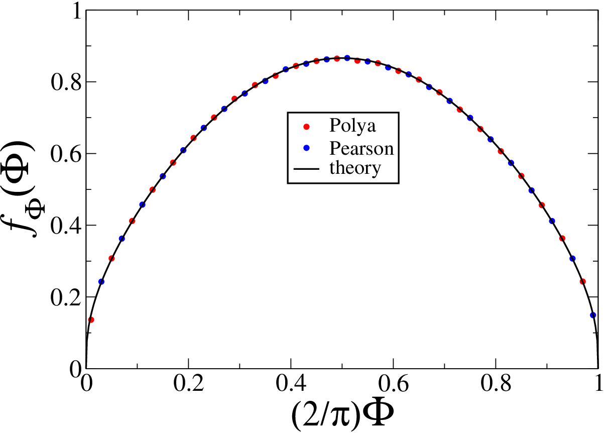
In the scaling regime of large times, the expression (3.10) demonstrates that is asymptotically a function of and , so that (3.19) becomes independent of . This is in agreement with the scaling law (3.6), implying that approaches
| (3.20) |
at large times. The ratio and the polar angle are therefore expected to have non-trivial asymptotic distributions, related to each other as
| (3.21) |
The symmetry (3.7), i.e.,
| (3.22) |
translates to the expected symmetry
| (3.23) |
From a quantitative viewpoint, using the scaling law (3.10) valid at large times, we can recast (3.19) into the form
| (3.24) |
where the accent denotes a derivative.
For generic values of the ratio , setting and in (2.9), with real, we obtain the following hyperbolic parametrization
| (3.25) |
of the function when runs over the imaginary axis. This yields after some algebra the following integral representation of , which is suitable for a numerical evaluation:
| (3.26) |
with
| (3.27) |
The dependence of the above result on the ratio is entirely encoded in the definition of the implicit function , such that
| (3.28) |
For , i.e., , we have . This is the only situation where the integral (3.26) is elementary, yielding
| (3.29) |
In the regime where the ratio is large, the most efficient route to derive the tail of consists in coming back to (3.24), using the asymptotic form , and changing variable from to . We thus obtain
| (3.30) | |||||
where the second integral is derived from the first one by performing an integration by parts and folding the contour onto the real axis. We thus obtain the power-law estimates
| (3.31) | |||
| (3.32) |
Figure 10 shows the distribution of the polar angle of the current record of Polya (red) and Pearson (blue) walks at time . Each dataset contains 50 bins. Every second bin of each dataset is plotted alternatively. Both histograms are in very good agreement with the asymptotic theoretical prediction (see (3.21), (3.26)), shown as a full curve. Corrections to scaling are too small to be detected.
4 Radial records
4.1 General analysis
This section is devoted to the statistics of radial records, shown as green symbols in Figure 1. At variance with diagonal and simultaneous records, investigated in Sections 2 and 3, radial records do not admit any recursive construction involving the hitting of translated copies of a target. In other words, there is no underlying simple renewal process.
The following analysis is therefore partly heuristic. Consider isotropic random walks consisting of discrete steps of unit length, in any dimension . Numerical simulations will be performed for Polya walks (simple random walks on the hypercubic lattice) and Pearson walks (steps having unit length and uniformly random orientations). Both kinds of walks obey , so that their diffusion coefficient reads
| (4.1) |
Let be the positions of the walker at the successive radial records, the corresponding radii, and the corresponding epochs. In other words, is the first position of the walker which lies outside the sphere with radius centered at the origin. For walks made of unit steps, we have
| (4.2) |
in full generality, with formally . For both kinds of walks, we have and . For Polya walks we have either or , whereas is an even integer, as the hypercubic lattice is bipartite in any dimension. For Pearson walks, can already take any value between 1 and 2.
For a fixed time , the number of simultaneous records is denoted as for short throughout Section 4. The radius
| (4.3) |
of the current radial record is nothing but the largest radius reached by the walk up to time .
At large times, the radius of the walk becomes the radius of a -dimensional Brownian motion. The latter process is known as a Bessel process of order . The largest radius becomes the maximum of that process up to time . Diffusive scaling implies
| (4.4) |
The reduced variables (associated with the radius of a generic point of the walk) and (associated with the current maximal radius of the walk) have universal distributions, which only depend on dimension . The distribution of is simply that of the radial part of an isotropic -dimensional Gaussian vector, normalized in accordance with (4.1). This reads
| (4.5) |
We have in particular
| (4.6) |
The distribution of the reduced variable is non-trivial. It is known in the form of an infinite series involving the zeros of the Bessel function in two dimensions [35, p. 280], and more generally in higher dimensions [35, p. 369].
The statistics of the number of radial records can be estimated as follows. The difference between the radii of any two successive records ought to average to some microscopic length (see (4.2))
| (4.7) |
It is therefore legitimate to expect that, for a given walk, the number of records and the largest radius are asymptotically proportional to each other, as
| (4.8) |
We thus predict the scaling laws
| (4.9) |
and in particular
| (4.10) |
with
| (4.11) |
The square-root growth law (4.10) is well-known in the one-dimensional case (see [11]). It was announced in (1.3) in the two-dimensional situation. It is actually super-universal, in the sense that it holds in any spatial dimension. This finding corroborates earlier numerical results in one, two and three dimensions [12].
4.2 Two dimensions
We begin by illustrating the above general results in the two-dimensional case. In this situation, the distribution of reads [35, p. 280]
| (4.12) |
where are the zeros of the Bessel function , growing as , whereas are the values of the Bessel function at these zeros. We have in particular
| (4.13) | |||
| (4.14) |
where is the modified Bessel function. These numbers are to be compared with and (see (4.6)).
Figure 11 shows numerical data for the mean number of radial records of Polya and Pearson planar walks, plotted against up to . Both datasets exhibit a very accurate square-root growth law. The slopes of the least-square fits shown as dashed lines, and the corresponding values of the distance according to (4.11), (4.13), are given in Table 3 for both kinds of walks.

| walk | ||
|---|---|---|
| Polya | 2.10 | 0.559 |
| Pearson | 2.35 | 0.500 |
Figure 12 shows the distribution of the number of radial records, , for Polya walks with steps. Numerical data (symbols) are in very good agreement with the distribution (4.12) of the rescaled variable (full curve). The constant of proportionality between and has been fixed by using the true finite-time mean record number . This procedure is numerically more accurate than using the asymptotic growth law (4.10). Corrections to scaling are again very small (of the order of one percent). This plot provides a strong corroboration of the expected law of proportionality (4.8).

For small values of , the distribution is dominated by the first term in (4.12), i.e.,
| (4.15) |
with and . This exponentially small left tail is to be contrasted with the distribution of the number of records for renewal processes (see (2.30), (2.31)). In that situation, the distribution of the rescaled variable is non-zero —and in fact maximal— at for all .
4.3 Higher dimensions
The general setting exposed in Section 4.1 and illustrated in two dimensions in Section 4.2 remains valid in any dimension. The aim of this section is to emphasize a few simplifying features at large dimensions.
First of all, as dimension increases, the asymptotic distribution of the radius becomes more and more narrow. We have indeed (see (4.6))
| (4.16) |
It is then clear that the distribution of the largest radius has the same property. In other words, as dimension increases, both rescaled variables and converge to the same deterministic value, which is unity, as in any dimension. This reads formally
| (4.17) |
Let us now turn to the geometrical arrangement of radial records. Figure 1 suggests that these records, shown as green symbols, occur in long worm-like sequences of consecutive points, interrupted by scarce non-local jumps. In order to elaborate on this observation, we introduce the angular correlation between the two most recent records at time , namely
| (4.18) |
(conditioned on having ). Figure 13 shows the angular correlation for Polya walks in dimensions , 4, 8 and 16 (see legend), plotted against up to . The dashed lines demonstrate a slow convergence of to unity, of the form
| (4.19) |
The amplitude of the leading correction is non-universal, i.e., depends on the kind of walk. Both for Polya walks (Figure 13) and for Pearson walks (not shown), is observed to decay slowly to zero, roughly proportionally to , as dimension increases.

The following picture therefore emerges in the regime of large spatial dimensions. Radial records occur in longer and longer worm-like sequences. The effect of non-local jumps between these sequences becomes negligible in large dimensions, as testified by the fall-off of the correction amplitude . The mean distance between the radii of successive records can therefore be estimated by considering an effective one-dimensional problem. The distances
| (4.20) |
between successive records of one-dimensional random walks have been investigated recently [11, 36]. They admit a non-trivial stationary distribution , depending on the whole step distribution defining the random walk. For a symmetric continuous distribution such that is convergent, their mean value has a simple universal expression [9, ch. XVIII.5]:
| (4.21) |
This result can be taken as a proxy for the distance . Using (4.1), this reads
| (4.22) |
Inserting this estimate into (4.11), and using (see (4.17)), we obtain the asymptotic expression
| (4.23) |
for the amplitude of the growth law (4.10) of the mean number of radial records. This prediction is expected to hold to leading order as for all walks consisting of unit steps.
Figure 14 shows the amplitudes of the growth law of the mean number of radial records of Polya and Pearson walks in all dimensions up to . Just as in the two-dimensional situation (Figure 11), amplitudes have been extracted by means of least-square fits of data in the range . These amplitudes are plotted against . Both datasets corroborate the scaling law (4.23) at large dimension, shown as a black straight line with slope . The difference between the amplitudes for Pearson and Polya walks is observed to decrease rapidly as a function of dimension and to reach a non-zero limit . This observation suggests that the first correction to the prediction (4.23) is finite and non-universal.

5 Discussion
In this paper we have investigated the statistics of various kinds of records associated with planar random walks. We have chosen three characteristic examples of records among many possibilities, namely diagonal, simultaneous and radial records. These examples are appealing and interesting in several regards. Their definition is simple and natural, involving only elementary geometrical considerations. The statistics of these records is varied. The mean numbers of records of each kind grow as power laws of time, with the simple rational exponents 1/4, 1/3 and 1/2.
The investigation of diagonal and simultaneous records of Polya walks, performed in Sections 2 and 3, relies upon the underlying renewal structure of the successive hitting times and locations of translated copies of a fixed target. In this sense, this work represents a two-dimensional extension of the analysis made by Feller of ladder points, i.e., records for one-dimensional random walks. Renewal theory has allowed us to derive by analytical means a vast panoply of results at large times, including the full statistics of the numbers of diagonal and simultaneous records (Section 2.3.2), the joint law of the epoch and location of the current diagonal record (Section 2.4), and the angular distribution of the current simultaneous record (Section 3.4). All these asymptotic results are universal, at least among the class of walks consisting of unit steps, whereas most of them extend to the whole class of isotropic diffusive walks.
Radial records of isotropic random walks in any spatial dimension have been investigated in Section 4. This study is partly heuristic, and thus different in spirit from the previous ones, for the mere reason that the sequence of radial records does not follow a renewal scheme. The mean number of radial records has been shown to follow a superuniversal law, growing as irrespective of dimension. The associated amplitude becomes itself universal at large spatial dimensions, growing as , irrespective of the kind of diffusive walk under consideration, at least for walks consisting of unit steps. The full statistics of the number of records has also been characterized.
The present work could be further extended in a great many directions. As stressed in Section 1, a whole breadth of different records can be attached to a planar random walk such as the Polya walk on the square lattice, besides the three cases we have chosen to explore in detail. Moreover, besides the isotropic diffusive walks considered in this work, many other types of random walks could be considered a priori, including anisotropic diffusive walks, walks possessing a drift velocity, Lévy walks whose step distribution has an infinite variance, and various kinds of walks with correlated steps.
To close, let us discuss how our main findings concerning isotropic walks are changed in higher spatial dimensions . The case of radial records has been studied in Section 4 and summarized just above. The statistics of diagonal and simultaneous records exhibits a more interesting dependence on . The definitions of both kinds of records extend in a straightforward way to Polya walks in any dimension, e.g. on hypercubic lattices, as well as the reduction of the problem to renewal processes. Now, let us remind the general fact that two objects of dimensions and embedded in -dimensional space intersect easily if , as their intersection is typically an object of dimension .22 2 This formula is an extension to generic objects of the well-known identity for linear subspaces . In the opposite case (), the objects intersect either scarcely or not at all. The situation where , i.e., , is the marginal one. Within this setting, let us first consider diagonal records. The target is the main diagonal of the lattice in the direction . The walk has , as a consequence of diffusive scaling, whereas the target has , so that the marginal situation is . The corresponding survival probability, which decays as for , can indeed be argued to decay as for , and to reach a non-zero escape probability for (see [28, 29, 37]). As a consequence, the mean number of records grows as for , whereas for the total number of records of an infinitely long walk is finite, and geometrically distributed with . The case of simultaneous records is equally interesting. There, the target is an orthant, or hyperoctant, whose tip is initially located at the point . The walk still has , whereas the target now has , so that both objects intersect easily in any dimension. The corresponding survival probability indeed decays as a universal power law of the form in any spatial dimension , where the survival exponent only depends on [28]. We have , , [38], and is known to become exponentially small for large [28, 29]. Thus, in any spatial dimension , the mean number of records grows as , and its full distribution is universal and given by renewal theory. Table 4 summarizes the above discussion.
| Records | |||
|---|---|---|---|
| Diagonal | finite | ||
| Simultaneous | |||
| Radial |
Appendix A Additive and multiplicative observables in renewal theory
This Appendix is devoted to the evaluation of additive and multiplicative observables attached to a renewal process in continuous time. Notations are consistent with those used in the body of the paper. In particular, renewal events are referred to as records. Within this setting, many time-dependent quantities can be determined explicitly in Laplace space. Hereafter we adopt the line of thought and the notations of our earlier work [31]. Let the temporal increments be iid variables drawn from a continuous distribution with density . For a given time , the number of records is the unique integer such that , with the definition
| (1.1) |
The number of records is random, as it depends on the whole renewal process .
Additive observables
An additive observable is a quantity of the form
| (1.2) |
where is an arbitrary given function of the temporal increment . The definition of may involve averaging over other random variables, as long as they are statistically independent of . A renewal process endowed with an additive observable of this kind is referred to as a renewal reward process [19]. Continuous-time random walks [39] belong to this class of processes.
The quantity can be evaluated as follows. We have
| (1.3) |
where is a shorthand for and denotes the indicator function of an event. In Laplace space, this translates to
| (1.4) |
Averages over the iid variables boil down to two simple integrals, i.e.,
| (1.5) |
We thus obtain
| (1.6) |
The simplest of all additive observables, corresponding to the choice
| (1.7) |
yields , the mean number of records at time . We have then , so that (1.6) becomes (2.24), as should be.
Consider now the power-law observable
| (1.8) |
and a distribution with a power-law tail of the form
| (1.9) |
The range of exponents of interest for the present purpose is
| (1.10) |
For instance, diagonal and simultaneous records respectively correspond to and , whereas the exponent dictated by diffusive scaling provides a toy model for the abscissa of the current record. All over the parameter range (1.10), we obtain the estimates
| (1.11) |
for , so that
| (1.12) |
We thus predict a power-law growth of the form
| (1.13) |
This result is universal, in the sense that it only involves the exponents and .
Non-universal asymptotic results show up outside the self-similar range (1.10). Let us just give one example. For , the estimate (1.11) for is to be replaced by the non-universal constant
| (1.14) |
so that we have
| (1.15) |
At variance with (1.13), this result is non-universal, as it involves the ratio of two microscopic constants and .
Multiplicative observables
A multiplicative observable is a quantity of the form
| (1.16) |
where is an arbitrary given function of the temporal increment . Here again, the definition of may involve averaging over other random variables, as long as they are statistically independent of .
The quantity can be evaluated as follows. We have
| (1.17) |
In Laplace space, this translates to
| (1.18) |
Averages over the iid variables again boil down to two simple integrals, namely and
| (1.19) |
We thus obtain
| (1.20) |
The simplest of all multiplicative observables, corresponding to the choice
| (1.21) |
where is an arbitrary constant, yields
| (1.22) |
the generating function of the probabilities . We have then , so that (1.20) reads
| (1.23) |
The expression (2.21) is recovered by expanding the above result as a power series in , as should be.
Appendix B Derivation of Equation (2.49)
This Appendix is devoted to the derivation of (2.49) for an arbitrary survival exponent in the range . The essential part of the derivation consists in evaluating the expression (see (2.48))
| (2.1) |
Using the power-law tail (2.7) of and the distribution (2.17) of , this reads
| (2.2) | |||||
Changing variables from to and from to , and introducing the dimensionless variable , we obtain
| (2.3) | |||||
The integration over can be performed first, yielding
| (2.4) |
where is the modified Bessel function. The integration over can also be worked out. We thus obtain
| (2.5) |
with
| (2.6) |
Inserting the estimates (2.47) and (2.5) into (2.46), we obtain
| (2.7) |
where the scaling variables and read
| (2.8) |
and the scaling function is given in parametric form by
| (2.9) |
The point corresponds to , so that , as should be.
Whenever is rational, the scaling function is an algebraic function. More precisely, for in irreducible form, with (since ), the algebraic degree of is (if is odd) or (if is even).
There is one single case in degree 2. This is , corresponding to diagonal records investigated in Section 2. We have
| (2.10) |
hence the explicit expression
| (2.11) |
Two cases pertain to degree 3. The first one is , corresponding to simultaneous records investigated in Section 3, where we obtain the equation of a cubic curve:
| (2.12) |
This curve is said to be unicursal, as it admits the rational parametrization
| (2.13) |
The second case in degree 3 is , where we have
| (2.14) |
Appendix C Law of the ratio of two correlated random variables
In this Appendix we investigate the distribution of the ratio
| (3.1) |
of two positive random variables with an arbitrary joint distribution.
Consider first the case where the density of the joint distribution is known. We have then
| (3.2) | |||||
Consider now the case where only the bivariate characteristic function
| (3.3) |
of the joint distribution is known. We have then
| (3.4) |
and so (formally)
| (3.5) |
Let us assume for a while that the density falls off exponentially in both variables, so that is analytic when and are both larger than for some positive . We can therefore choose and to be small and negative. The integral over then reads , whereas the integral over is given by the residue at the double pole at . We thus obtain
| (3.6) |
The above expression makes sense for an arbitrary joint distribution . The integration contour can indeed be chosen to be the imaginary axis, so that (3.6) only involves the bivariate Fourier transform of .
Whenever the variables and are exchangeable, i.e., or , the product
| (3.7) |
is invariant under the change of into its inverse.
Let us illustrate the above by considering the example where and are two identical independent Lévy stable variables with index in the range and a suitable chosen scale factor, such that
| (3.8) |
Equation (3.6) then reads
| (3.9) |
Setting and dealing separately with the ranges and , some algebra leads us to the expression
| (3.10) |
We have thus recovered the celebrated Lamperti law [40]. The above expression obeys the symmetry (3.7), as should be.
References
References
- [1] Chandler K N 1952 J. Roy. Statist. Soc. - Series B 14 220–228
- [2] Foster F G and Stuart A 1954 J. Roy. Statist. Soc. - Series B 16 1–13
- [3] Rényi A 1962 Ann. Sci. Univ. Clermont-Ferrand 8 7–13
- [4] Glick N 1978 Amer. Math. Monthly 85 2–26
- [5] Arnold B C, Balakrishnan N and Nagaraja H N 1998 Records (New York: Wiley)
- [6] Nevzorov V B 2001 Records: Mathematical Theory (Translation of Mathematical Monographs vol 194) (Providence, RI: American Mathematical Society)
- [7] Bunge J and Goldie C M 2001 Handbook of Statistics 19 277–308
- [8] Feller W 1957 An Introduction to Probability Theory and its Applications 2nd ed vol 1 (New York: Wiley)
- [9] Feller W 1971 An Introduction to Probability Theory and its Applications 2nd ed vol 2 (New York: Wiley)
- [10] Wergen G 2013 J. Phys. A 46 223001
- [11] Godrèche C, Majumdar S N and Schehr G 2017 J. Phys. A 50 333001
- [12] Edery Y, Kostinski A and Berkowitz B 2011 Geophys. Res. Lett. 38 L16403
- [13] Polya G 1919 Mitt. der Phys. Ges. Zürich 19 75–86
- [14] Pearson K 1905 Nature 72 294
- [15] Spitzer F 2001 Principles of Random Walk (New York: Springer)
- [16] Weiss G H 1994 Aspects and Applications of the Random Walk (Amsterdam: North-Holland)
- [17] Hughes B D 1995 Random Walks and Random Environments. Volume 1: Random Walks (Oxford: Clarendon)
- [18] Dynkin E B 1961 Selected Translations Math. Stat. Prob. 1 171 [Izv. Akad. Nauk. SSSR Ser. Math. 19, 247 (1955)]
- [19] Cox D R 1962 Renewal Theory (London: Methuen)
- [20] Cox D R and Miller H D 1965 The Theory of Stochastic Processes (London: Chapman & Hall)
- [21] Bousquet-Mélou M 2016 J. Combin. Theory - Series A 144 37–79
- [22] Raschel K and Trotignon A 2019 Elec. J. Combinatorics 26 P3.31
- [23] Sommerfeld A 1894 Math. Annalen (Leipzig) 45 263–277
- [24] Redner S 2001 A Guide to First-Passage Processes (Cambridge: Cambridge University Press)
- [25] Comtet A and Desbois J 2003 J. Phys. A 36 L255–L261
- [26] Lagache T and Holcman D 2008 SIAM J. Appl. Math. 68 1146–1167
- [27] Dy D L L and Esguerra J P 2008 Phys. Rev. E 78 062101
- [28] Ben-Naim E and Krapivsky P L 2010 J. Phys. A 43 495007
- [29] Ben-Naim E and Krapivsky P L 2010 J. Phys. A 43 495008
- [30] Chupeau M, Bénichou O and Majumdar S N 2015 Phys. Rev. E 91 032106
- [31] Godrèche C and Luck J M 2001 J. Stat. Phys. 104 489–524
- [32] Scher H and Montroll E W 1975 Phys. Rev. B 12 2455–2477
- [33] Barkai E 2001 Phys. Rev. E 63 046118
- [34] Penson K A and Górska K 2010 Phys. Rev. Lett. 105 210604
- [35] Borodin A N and Salminen P 1996 Handbook of Brownian Motion - Facts and Formulae (Basel: Birkhäuser)
- [36] Godrèche C, Majumdar S N and Schehr G 2016 Phys. Rev. Lett. 117 070601
- [37] Krapivsky P L and Redner S 2010 J. Stat. Mech. P11028
- [38] Bogosel B, Perrollaz V, Raschel K and Trotignon A 2020 J. Combin. Theory - Series A 172 105189
- [39] Montroll E W and Weiss G H 1965 J. Math. Phys. 6 167
- [40] Lamperti J 1958 Trans. Amer. Math. Soc. 88 380–387