Noncausal Page-Wootters circuits
Abstract
One of the most fundamental open problems in physics is the unification of general relativity and quantum theory to a theory of quantum gravity. An aspect that might become relevant in such a theory is that the dynamical nature of causal structure present in general relativity displays quantum uncertainty. This may lead to a phenomenon known as indefinite or quantum causal structure, as captured by the process matrix formalism. Due to the generality of that framework, however, for many process matrices there is no clear physical interpretation.
A popular approach towards a quantum theory of gravity is the Page-Wootters formalism, which associates to time a Hilbert space structure similar to spatial position. By explicitly introducing a quantum clock, it allows to describe time-evolution of systems via correlations between this clock and said systems encoded in history states.
In this paper we combine the process matrix framework with a generalization of the Page-Wootters formalism in which one considers several agents, each with their own discrete quantum clock. We describe how to extract process matrices from scenarios involving such agents with quantum clocks, and analyze their properties. The description via a history state with multiple clocks imposes constraints on the implementation of process matrices and on the perspectives of the agents as described via causal reference frames. While it allows for scenarios where different definite causal orders are coherently controlled, we explain why certain non-causal processes might not be implementable within this setting.
I Introduction
Indefinite causal structure is an extension of the usual notion of causal structure that is expected to become relevant in quantum gravity: In general relativity, causal structure is dynamical instead of fixed and attributing quantum properties Hardy 2005; Hardy 2007; Hardy 2009; Feynman 2011; Zych et al. 2019; Rovelli 2004; Kiefer 2012; Butterfield and Isham 2001 would imply the existence of exotic causal structures, like superpositions of space-times and superpositions of the order of events. The process matrix framework Oreshkov et al. 2012; Araújo et al. 2017 was invented to systematically describe such indefinite or quantum causal structures. However, many processes that arise in this framework have no clear physical interpretation and it is not known which of them are realizable in nature. It has, therefore, been suggested that only processes, which reversibly map a well defined causal past to a well defined causal future with possibly indefinite causal order in between, are physical Araújo et al. 2017.
For such processes, it has been shown that one can always find a causal reference frame that represents the perspective of an agent within the causal structure Guérin and Brukner 2018. While the agent’s event is local in their causal frame of reference, the events of other agents may be “smeared” over the causal past and future of the event. Still the question which processes are realizable in nature remains open.
Some non-causal processes can violate device-independent causal inequalities Branciard et al. 2015; Baumeler et al. 2014; Brukner 2015, although no physical interpretation for such processes are known. Other processes, for example the so-called quantum switch Chiribella et al. 2013; Procopio et al. 2015; Rubino et al. 2017a, where the order of operations is controlled by a quantum system, cannot violate causal inequalities but exhibit indefinite causal order that can be identified by causal witnesses Araújo et al. 2015. Moreover, it is possible to experimentally implement such coherent quantum control of causal order Procopio et al. 2015; Rubino et al. 2017a; Wei et al. 2019; Goswami et al. 2020; Taddei et al. 2021; Rubino et al. 2017b; Goswami et al. 2018; Guo et al. 2020. Overall, however, many mathematically consistent process matrices are believed to be unphysical, yet there are only very few reasonable postulates, like Araújo et al. 2017, that actually allow to rule out some processes as unphysical.
A crucial obstacle in finding a complete theory of quantum gravity is caused by the different role of time in general relativity and quantum theory. As an approach to bridge this conceptual gap, one can use a timeless formalism Page and Wootters 1983; Unruh and Wald 1989; Rovelli 1990; Reisenberger and Rovelli 2002; Hellmann et al. 2007; Giovannetti et al. 2015; Höhn and Vanrietvelde 2020; Höhn 2019; Hoehn et al. 2019; Hoehn et al. 2020; Castro-Ruiz et al. 2020, which we refer to as the Page-Wootters formalism in this paper. In this formalism, one also associates a Hilbert space with time, which can be interpreted as a quantum clock. One describes the physics of the extended system including the clock by using history states which are obtained via a Wheeler-DeWitt-like equation using a constraint operator. These history states encode dynamics as correlations between the main system and the quantum clock.
In Ref. Castro-Ruiz et al. 2020, the authors considered a generalized Page-Wootters approach using several clocks. The authors found that history states arising from solving a Hamiltonian constraint for gravitationally interacting clocks can give rise to indefinite causal order and studied the time evolution according to the perspectives of different clocks. In particular, they showed how the Page-Wootters formalism can recover the so-called gravitational quantum switch Zych et al. 2019. Their approach works for important examples, but it is not clear in general which process (if any) is implemented by a given history state, or what is the set of non-causal processes that can be implemented within such a framework.
The observations in Castro-Ruiz et al. 2020 motivate us to investigate the relation between causal order and several quantum clocks in further detail, and develop a full framework that systematically combines the process matrix and the Page-Wootters formalism. A refined description of indefinite causal structure that explicitly models the agents’ perceptions of time might help to discover physical scenarios that give rise to indefinite causal structure. In particular, a well-defined combination of these two approaches might lead to new consistency conditions that allow to rule out some process matrices as unphysical.
Even beyond the search for criteria for physical process matrices, the combination of process matrices with the Page-Wootters formalism is an interesting topic by itself. Both frameworks can be seen as approaches towards quantum gravity. However, so far they were mostly isolated and independent from each other, although they are not incompatible. The Page-Wootters formalism can be regarded as an independent formulation of quantum theory, similar to the path-integral formulation. It is an interesting question which processes can be naturally implemented within a particular formulation of quantum theory. It is known that any quantum circuit (i.e. a definite causal order) can be implemented within the Page-Wootters formalism as a Feynman’s quantum computer and a single (i.e. global) quantum clock Feynman 1985; Kitaev et al. 2002; Breuckmann and Terhal 2014; Caha et al. 2018. Can the formalism also account for more general causal structures such as coherently controlled causal orders or even those that lead to the violation of causal inequalities?
To approach this question, in the present paper, we present a general definition of what it means for a history state to implement a pure process matrix Araújo et al. 2017, for the case of finite dimensional systems and many clocks.
We describe how to extract the agents’ perspectives from the history states, which corresponds to a refinement of the concept of causal reference frames Guérin and Brukner 2018 that explicitly includes the quantum clocks. We show that arbitrary coherently controlled causal order can be extracted from our framework when different clocks tick at different rates (for example, due to time dilation effects). Moreover, we analyze the additional restrictions that the history states impose on the extracted process matrices. These restrictions might be regarded as reasons why some processes cannot be implemented in nature. While the Page-Wootters formalism with many clocks can enable the extraction of processes with definite causal order and quantum controlled causal order, it additionally provides insights into why some processes might not be realizable within the framework.
We consider discrete instead of continuous clocks because this allows us to express the perspectives of the agents using circuits. Our approach does not start by defining a constraint operator and solving it; instead we work directly at the level of history states. We develop a systematic framework that combines process matrices and Page-Wootters history states with several discrete clocks. We describe how to model scenarios where these clocks are associated with agents that are initially all part of a definite space-time causal structure. Then the agents might enter a ”region” of quantum causal structure, where the global order of events is no longer well defined. At the end, however, all agents return to a definite causal structure.
The paper is structured as follows: We first recapitulate important aspects of the process matrix formalism (including causal reference frames) and the Page-Wootters formalisms in Sections II and III before we motivate and introduce our framework, which combines these two approaches, in detail in Section IV. In that context, we derive several mathematical properties of our setting, in particular restrictions on process matrices. In Section V, we first construct examples involving varying clock speeds and indefinite causal structure before we show how to implement arbitrary quantum-controlled causal order in our setting. At the end of Section V we discuss why another well-known, non-causal process might not be implementable in our framework. Finally, we discuss our findings in Section VI.
II Process matrices and causal reference frames
In this section we give a short introduction to the operational setting of the process matrix formalism and explain the parts of the framework that are important for the rest of the paper.
The basic operational setting of the process matrix formalism concerns several agents (here of them), labeled , each of them inside their own (small) laboratory where the usual rules of quantum theory are valid. The outside “environment”, which relates the various agents, is not assumed to be causally definite, for example it could be a superposition of space-time structures. During the protocol, each agent receives a quantum system from the “environment”, applies a quantum instrument i.e. a probabilistic quantum channel (for example a measurement or a pure quantum channel) to that system and then sends it out again. This well defined local time ordering inside the laboratory can be thought of as being tracked by a clock associated with each agent, the bipartite case is depicted in Figure 1(a).
The process matrix is the mathematical object that encodes the observed outcome probabilities for any choice of local quantum instruments. Process matrices describing definite causal order, i.e. the global order of operations performed by different agents is well defined, are equivalent to higher order quantum maps or quantum combs Chiribella et al. 2008; Perinotti 2017; Bisio et al. 2011; Chiribella et al. 2009; Yokojima et al. 2021. In general, however, they allow scenarios with indefinite causal order, where no such global order exists, and are in that sense generalizations of quantum combs.
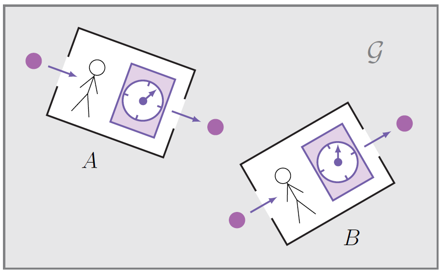

In Araújo et al. 2017, processes (called quantum superchannels in Yokojima et al. 2021) are formalized as maps from a global past to a global future, that depend on the agents’ operations.
In addition to the agent’s systems, whose Hilbert spaces are labeled , we introduce ancillary systems . The ancillary system can be used, for example, as a quantum memory recording a measurement outcome. Each agent is allowed to act with a quantum channel on their system and their ancilla, i.e. a completely positive trace-preserving map (CPTP) . One assumes that the ancillas have trivial evolution except when the respective operations of the agents are applied. Then, a process (or quantum superchannel) is a multilinear map that maps the agents’ quantum channels to a quantum channel, while acting as the identity on all the ancillary systems (just as in Figure 1(b), but with the unitaries replaced by quantum channels). This map encodes the causal structure given by the environment.
In this paper, we only consider pure processes.
Using Stinespring’s dilation theorem Stinespring 1955; Nielsen and Chuang 2000 one can represent the quantum operations of the agents as unitaries acting on the respective system and ancilla that the agents obtain from the environment. The ancillas serve as both purifying systems and as memories recording the outcomes. We say that a process is a pure process if it is a unitary preserving map, i.e. is unitary for any unitaries , while acting as the identity on the ancillary systems. The basic mathematical structure of a bipartite pure process is depicted in Figure 1(b).
Since many non-causal process matrices lack a clear interpretation and it is not clear whether they are compatible with the known physical laws, it has been suggested that only purifiable processes, which means they can be obtained from pure processes, are physical Araújo et al. 2017. Such processes can be regarded as reversible transformations from a well defined causal past to a well defined causal future, with indefinite causal order in between. We note that the quantum-switch is an example of a pure process, as shown explicitly in Araújo et al. 2017, and it is physically realizable either in gravitational Castro-Ruiz et al. 2020; Zych et al. 2019 or optical setups Procopio et al. 2015; Rubino et al. 2017a; Wei et al. 2019; Goswami et al. 2020; Taddei et al. 2021; Rubino et al. 2017b; Goswami et al. 2018; Guo et al. 2020.
The notion of causal reference frames Guérin and Brukner 2018 was introduced as an equivalent description of the pure process matrix formalism. The causal reference frame represents the perspective of an agent inside a (possibly indefinite) causal structure. More concretely, one imagines the perspective of an agent, say , as follows: The crucial moment for agent is when he or she applies unitary . The evolution starting from the beginning of the protocol up to that moment is described by a unitary , which is called the causal past of and can depend on the instruments of all other agents. Then enforces time evolution via on the input to his or her laboratory and the ancilla , while all other degrees of freedom evolve in an uncorrelated way. The evolution of these other degrees of freedom can be absorbed into such that without loss of generality we can assume that during ’s time of action, evolution is given by . Afterwards the evolution up to the end of the protocol is described by a unitary , which is called the causal future of . It can again depend on the instruments of all other agents. As shown in Ref. Guérin and Brukner 2018 all pure processes admit a decomposition in causal reference frames, i.e. if is a pure process, then can be written as
| (1) |
where are unitaries that depend on all unitaries other than and that describe the time-evolution according to ’s point of view. A similar decomposition exists from the point of view of all other agents. In the present paper we take a similar approach, but we make the addition of a localized quantum clock associated to each agent, and explain how the perspectives of various agents can arise from a perspective neutral history state as given by the Page-Wootters formalism.
III The Page-Wootters formalism
In this section we give a brief general overview of the Page-Wootters formalism for continuous as well as discrete quantum clocks. A possible justification for considering quantum clocks with discrete Hilbert spaces comes from arguments involving the Bekenstein bound Bekenstein 1973 that Hilbert space is fundamentally finite-dimensional Garay 1995; Bao et al. 2017. Also, it can be argued that all information that can ever be acquired via measurements is finite and that therefore on the fundamental level physics should be discrete as well and indeed, finite Gisin 2019. Furthermore, we get significant technical simplifications due to the fact that for finite-dimensional Hilbert spaces, the physical Hilbert space is a subspace of the kinematical Hilbert space, while this is not the case for infinite dimensional Marolf 2002; Hoehn et al. 2019.
Most importantly for our purpose, the assumption of finite dimensional clocks allows us to get a physical picture of indefinite causal structure in form of generalizations of quantum circuits.
In addition to the usual system Hilbert space the Page-Wootters formalism introduces an additional Hilbert space associated with time that can be interpreted as an ideal quantum clock. In analogy to position in non-relativistic quantum mechanics can be chosen to be spanned by square integrable functions on the real line; informally it is common in physics to imagine this Hilbert space as . In analogy to the usual momentum operator, one can define an operator as the generator of translations on . In the time representation, i.e. , it is given by . Let be the Hamiltonian of the system and consider the constraint operator . Let be a state on that satisfies the Wheeler-DeWitt-like constraint equation . Such states are often called physical states. Without worrying about normalizability, one can formally expand by using the time basis as
| (2) |
With this expansion it becomes clear why states are also called history states: For each time , they encode a system state and an ordered time sequence corresponds to the history of the state given by and . Plugging the expansion Eq. (2) into the constraint equation, one can show that the system state satisfies
| (3) |
which is the standard Schrödinger equation. Therefore, this approach recovers the usual quantum formalism. In general, solutions to the constraint equation can be obtained via an operator
| (4) |
which gives a valid physical (or history) state, i.e. solution to the constrain equation , when applied to arbitrary states . For this reason the operator is sometimes called the physical projector Dolby 2004, although it is not a projector in the strict mathematical sense.
Moreover, is a unitary operator on and in case of there being no interaction term between clock and system, i.e. , it can be shown that it gives the time evolution according to the Schrödinger equation, i.e. .
The Page-Wootters formalism has been adapted to regular (i.e. causal) quantum circuits, see for example Feynman 1985; Kitaev et al. 2002; Breuckmann and Terhal 2014; Caha et al. 2018. It uses one finite dimensional quantum clock and is described by the constraint equation
| (5) |
where the Hamiltonians
| (6) |
can be understood as making the clock tick once and applying some unitary to the system. In other words, at time the circuit applies gate . Solutions to Eq. (5) are history states of this quantum circuit in the form
| (7) |
with being the circuit’s input, see Fig. 2. When projecting the clock onto the final time the system is in the state , which corresponds to the output of the circuit under consideration. While it is not straightforward to write a physical projector analogous to the continuous case in Eq. (4), we can define a projection operator onto the space of solutions to the constraint equation by
| (8) |
where the are given according to Eq. (7) with initial states taken from an orthonormal basis for . is the projector onto the space of physical states, which contrarily to the continuous case is now a proper subspace of . Note that similarly to the continuous case we can relate the physical projector to the unitary evolution of the circuit between the respective times by
| (9) |

In what follows we will associate a discrete clock with each agent which gives rise to history states of the form
| (10) |
where is the initial state of the system. Intuitively, the matrices encode what happens to the system between the initial time and the time when the collection of clocks shows the respective values. By projecting onto a certain clock state we will obtain conditional or perspectival states that correspond to the state agent assigns to everything other than their own clock at time . In the next section we present what we consider reasonable physical assumptions the conditional states and hence the history state have to fulfill.
We will almost exclusively consider the history states as they explicitly represent the perspectives of the agents and the systems and we can directly impose physical requirements on them. The constraint operator can then be implicitly defined afterwards as an operator that annihilates this family of history states. Whether this constraint operator has a simple form, or has desirable properties such as locality, is an interesting question that is nevertheless not pursued in this paper.
IV Process matrices within a timeless formalism
IV.1 The operational setting and postulates
In this section, we develop our framework that allows to model experiments described by pure process matrices within a generalized Page-Wootters approach.
As in the pure process matrix formalism we will describe scenarios with multiple agents being parts of a well-defined standard global causal past and future. In addition to the usual process matrix approach, the progress of time within the agents’ laboratoriess is described by quantum clocks with Hilbert spaces . We refer to the set of all clock variables collectively as . The idea of a well defined global, causal past and future common to all agents is formalized by the assumption that at the beginning as well as at the end of the protocol all the clocks experience at least one well-synchronized time step, see Fig. 3(a). During the protocol, each agent applies his or her quantum instrument on a part of a system which is common to all agents. As done in Araújo et al. 2017 we will assume that each agent has access to an ancillary degree of freedom, denoted by Hilbert spaces of unspecified dimension, to implement their quantum instrument. This ancillary system allows to represent the quantum instrument as a unitary within our pure history state approach. The ancilla acts as the environment for a dilation and as memory recording measurement outcomes. We assume that the ancilla systems are initialized to that they have trivial time evolution, except at the moment when the corresponding quantum instrument is applied. We collectively label the ancillas as .
In addition to the agents, their ancillas and quantum clocks, we also consider another quantum system that participates in the protocol, described by a Hilbert space . This quantum system represents the degrees of freedom that play an active role in the protocol, but are not directly associated with the agents or their laboratories. As in the formalism for pure processes, we assume that this quantum system is an input to the causal structure from the global past. We will often call it the main system and we denote its initial state by .
Hence our history states live on . We assume that the clocks are initialized to time at the start of the protocol and show times at the end. Then our history states can be expanded in the form
| (11) |


Now we can formalize our requirements on the timeless state describing the protocol depicted in Fig. 3. As mentioned before all clocks and ancillas are initialized to the states and, therefore, we can write:
- S.1
, where is a fixed ancillary state and is an arbitrary state of the system.
At the beginning and end of the experiment, physics should be given by a standard space-time causal structure. Hence, at the beginning and in the end, we assume the clocks of the agents are well-synchronized. In particular the clocks perform at least one synchronized step before and after they are part of any exotic causal structure. We further assume that during these initial and final well-synchronized time-steps nothing happens to the main system and formulate this in terms of agent for the sake of readability. Note that this does not conceptually single out agent but can equally be written for any of the agents.
- S.2
only for and only for and furthermore and
.
Analogous to the pure process matrices formalism described in Section II, we model the input from the environment as parts of the main system, i.e. we assume that the input to agent lives on a subspace , and ’s quantum instrument is described by a unitary which acts on the received part of the main system and ’s ancilla, i.e. acts on .
Note that different do not need to be different or orthogonal, in fact all of them might even be the full main system Hilbert space .
Next, we discuss the aspect of our discrete clocks formalism that differs the most from the continuous case, and justify the introduction of normalisation operators in order to relate the timeless state with the local perspective of the agents. As in Ref. Castro-Ruiz et al. 2020 we condition the history state on ’s clock showing time , i.e. , to describe what agent sees at time . In principle, the inner product in the kinematical Hilbert space is not necessarily the same as the inner product for the Hilbert space associated to the perspective of agent Hoehn et al. 2019. Indeed in the usual Page-Wooters formalism with infinite dimensional systems, the physical Hilbert space is not a proper subspace of the kinematical Hilbert space; this necessitates to define a new inner product for the perspectival states. Moreover, even in the finite-dimensional setting that we study here, in scenarios involving clocks with varying relative ticking speeds, one runs into normalization issues if one simply uses the kinematical inner product for the perspectival states. To see this, consider (temporarily switching to continous clocks to illustrate our point) the example of the history state in which one clock runs twice as fast as the other 11 1 We will not worry here about our use of non-normalisable states in the infinite dimensional case. For ’s perspective we find . However, for ’s perspective we find
where the prefactor comes from the measure via the change of the integration variable. In this example, the clock ticking rates are constant. However, in general the rates might change dynamically and the corresponding prefactor will depend on time. Hence, different agents will need different renormalizations, which in the infinite dimensional case can be accounted for in the definition of the inner products for the perspectival states. For the finite dimensional case with discrete clocks this motivates the introduction of normalization operators in order to relate the normalization of the bipartite history state with the normalization of the time-dependent perspectival states. Normalization issues for discrete clocks related to the process of discretization itself are discussed in detail in Appendix A.
We assume that the state agent sees at time is
| (12) |
where is the normalization operator that relates the perspective-neutral description to the perspective of agent at time . Here, is the Hilbert space formed by all clocks except the clock of agent .
A priori, the normalization operators make this approach extremely general. In principle, they could give us any state that we want. Therefore it is important that we impose some extra conditions. First of all, as the normalization operators generalize normalization constants, they should be linear, positive and invertible. Moreover, we wish that all the relevant physics concerning the initial system state and the agents’ operations is encoded in the history state, not the normalization operators. The normalization operator should just correct the normalization depending on the clocks. Therefore, we demand that the operators are independent of the initial system state and the choice of quantum instruments by the agents.
- N.1
is an invertible, linear, positive operator. It is independent of the input state and the local operations .
Without the latter restriction, one could use to introduce copies of the initial state or apply copies of the agents’ instruments to violate the no-cloning principle. We further assume that the normalization operator does not perturb how one agent sees the clocks of the other agents:
- N.2
The normalization operator has the form
(13) where the sum is taken over all clocks except the clock of agent , which is omitted, as indicated by . The operator is a linear, invertible and positive operator acting on (but not on the ancillas ).
This assumption is motivated by the requirement that the history state should represent the relevant physics and relations of the clocks. As their name implies, the normalization operators should adjust the normalization, but not introduce new clock physics.
Our previous requirement of well-synchronized clocks at the beginning and end of the experiment additionally implies that the respective normalization operators should just be identity operators.
- N.3
as well as .
Finally, we have to explain how the perspectival states are related to each other. We will assume that each agent sees a unitary time evolution as dictated by quantum theory in a pure state framework. This means we assume that for all there exists a unitary operator such that
| (14) |
Furthermore, just like in usual quantum theory, should not depend on the initial system state .
- U.1
is a unitary operator, independent of the initial state .
Moreover, time-evolution from to to is the same as time-evolution from to .
- U.2
, .
Next we discuss the crucial assumption that connects our framework to the formalism of pure processes. In the process matrix framework, one assumes that during the protocol each agent eventually receives a quantum system from the environment. We will assume that each agent is promised that they will receive this quantum system at a specific time . As explained before, we model that quantum system to be a part of the main system, described by subspaces of the main system space . Each agent acts with their local operation on that system and their ancilla (i.e. ) and then sends out the system at . In particular, this is the only time the agents use their quantum instrument. While the agents enforce evolution via their instrument, the remaining degrees of freedom should evolve in an uncorrelated way. This leads us to our final requirement, which is analogous within our framework to the existence of a causal frame decomposition Eq. (1) of process matrices.
- U.3
’s quantum instrument is used at the so called time of action , i.e.
(15) Furthermore at other times the evolution operator is independent of and only acts as the identity on the ancilla of , i.e. on .
Our assumptions introduce a transformation that maps the initial state to the final state . This transformation depends on the agents’ actions and is visualized in Fig. 3. Our last assumption is that this transformation can be extended to a full process Araújo et al. 2017 i.e. quantum superchannel Yokojima et al. 2021. This means that it must be possible to interpret the quantum causal structure as a process, even if we describe the agents’ operations as channels instead of (purified) unitaries.
We make the assumption that our Postulates S.2, N.1, N.2, N.3, U.1, U.2 and U.3 continue to be satisfied if the ancillary systems are initialized to states other than , and that we can continue to use the same normalization operators and perspectival time evolutions as for the initialization . This is no substantial conceptual restriction, because none of these postulates explicitly refers to any particular initial ancillary system state. Postulate S.1 just defines the particular choice of initialization for the protocol.
This concludes the description of the operational setting and of our assumptions. We will subsequently investigate the mathematical and physical implications of our setting and postulates.
IV.2 History states lead to pure processes
First, we show that the evolution of the main system and the ancillas must be given by a pure process. For that purpose we have to analyze the relation between the initial and the final state, in particular with respect to the operations of the agents. This can be done by taking the perspective of an agent, for example , and applying our unitary time evolution postulates:
| (16) |
We can define a map that describes how the final system and ancilla state is related to the initial state:
| (17) |
Eq. (16) shows that is a unitary that maps the initial system and ancilla state to the final state and that it is multilinear in the local operations. Furthermore, this decomposition shows that the only change in the state of the ancilla of is caused by ’s local operation. We assumed that this map can be extended to a full process. We conclude that is a pure process as defined in (Araújo et al. 2017; Yokojima et al. 2021) with the difference that Eq. (16) represents a refined causal reference frame decomposition that explicitly includes the quantum clocks, compare to Eq. (1).
The fact that we obtain pure processes has important consequences: According to Barrett et al. 2021; Yokojima et al. 2021, in the bipartite case our setting implies that no violation of device-independent causal inequalities can occur: The bipartite pure process can only be causally ordered or quantum-controlled causal order.
IV.3 Additional restrictions for the local perspectives of the agents
Let us further investigate the relation between our framework and the original causal reference frame framework of Guérin and Brukner 2018, in particular the relation between Eqs. (1) and (16), in further detail. Both frameworks work with purifications, in particular the actions of the agents are described by purified unitaries and the relevant process matrices turn out to be the pure processes. The crucial objects of the causal reference frame framework are the unitaries that describe the past before and the future after an agent’s action. More specifically, from the point of view of agent , the evolution from the beginning of the protocol up to the time of ’s action is described by the unitary . In our framework, this unitary corresponds to . The evolution directly after ’s action up to the end of the protocol is described by , which in our framework corresponds to .
The crucial difference between our framework and that of causal reference frames is that we explicitly model the quantum clocks and explain how the agents’ perspectives arise from a perspective neutral history state. This gives us a refined description of the agents’ perspectives because we explicitly model individual time steps in between the beginning of the experiment, the time of action and the end of the protocol. In Ref. Guérin and Brukner 2018 the causal past and future unitaries and are allowed to be arbitrary as long as they combine to the pure process via Eq. (1). However, in our setting the history state induces further compatibility constraints on the perspectives of the agents.
We will now present one such constraint that is particularly restrictive: Affine-linearity in the operations of the other agents. Consider a history state as in Eq. (11). We can write
| (18) |
with
| (19) |
Similar equations hold for the other agents. From our assumptions, we can see that is constant in for and linear in for , because the same is true for . We can relate the time evolutions of two different agents (here and ) via
| (20) |
The dependence of on shows that is a sum of functions linear in or constant in , i.e. is affine-linear in . The same argument can be made for all other agents. Hence we get that any time evolution as seen by agent (with all clocks initialized to time ) has to be an affine linear function of the operations of all other agents. This affine linearity is a severe restriction and a potential obstacle for implementing some non-causal processes in this framework. In Section V.4 we will apply this insight to an example involving an exotic tripartite process Araújo et al. 2017; Baumeler and Wolf 2016 to see that a causal reference frame decomposition for this process in Ref. Guérin and Brukner 2018 is incompatible with our framework.
IV.4 Discrete constraint operators and physical projectors
Finally, we will briefly discuss constraint operators and physical projectors in our framework since they are among the main objects of interest in the Page-Wootters formalism presented in Section III. By construction, our history states form a subspace and by linearity, is the history state associated with the input state , as one can see e.g. from Eq. (18). Therefore, we can define a constraint operator as where is the orthogonal projector onto . Then the kernel of is given by .
We note that in general, in our framework cannot be written analogous to the case of a standard quantum circuit with one clock, see Eq. (8). More specifically, for an orthonormal basis , the corresponding history states
may fail to be orthogonal due to the normalization operators:
In that sense, the map from initial states to history states is not necessarily unitary, in contrast to the unitary evolution of the main system and ancilla state, see Eq. (17).
We can, however, write in a form more reminiscent of the original Page-Wootters framework, compare Eq. (4), as
| (21) |
where is an integer (we could take ). This can be seen by noting that is a hermitian matrix with only eigenvalues or . If is an eigenvector of with , we have , while if we have , showing . As discussed in Appendix B it is not clear whether in Eq.(21) can be linked to the perspectival unitaries similar to Eq. (9).
V Causal and non-causal Page-Wootters circuits
In this section we now apply our framework to give several examples of physical scenarios that go beyond the standard setting of circuits with well-synchronized clocks. First, in Section V.1, we consider a setup inspired by the famous twin paradox in which the clocks of two agents are still in a well-defined relation to each other, but tick at different rates. Afterwards, in Section V.2, we describe a scenario for the bipartite quantum switch as a prototypical example of a known class of non-causal processes. There, a control quantum system determines the tick rates of the agents’ clocks and more importantly the order of the agents’ operations. In Section V.3, we go beyond the example of the bipartite switch and show that arbitrary coherently controlled causal orders can be realized in our framework. Finally, in Section V.4, we consider an interesting pure, non-causal process that is further known to violate causal inequalities Baumeler and Wolf 2016; Baumeler et al. 2014; Araújo et al. 2017. We will argue that this process cannot be implemented as a superposition of classical histories and that the causal reference frame decomposition from Ref. Guérin and Brukner 2018 cannot be adapted to our setting.
V.1 A history state for a scenario with varying clock ticking rates
Our first example of an interesting process that fits into our setting but is not a standard circuit is inspired by the famous twin paradox. Specifically we consider a scenario that features varying clock speeds of two agents and where during the protocol the clock of one ticks slower than the clock of the other, reminiscent of the one twin that leaves earth traveling at relativistic speed and returns to find his or her sibling older than they are themselves.
Here the two agents act on subsystems and of the input quantum state with unitary operations and respectively. The causal order in this example is well defined and we consider the case where acts before . Moreover, between ’s and ’s time of action some global evolution of the system happens, which is independent of the two agents. In the beginning and at the end the agents’ clocks tick at the same speed, but in between the clock of ticks more slowly than that of . The scenario is depicted in Figure 4 and captured by the following history state .
| (22) |
where . The perspectival states for the two agents including the non-trivial normalization operators are
| (23) | ||||||

Note that the normalization operators are non trivial for precisely those times where the clock of ticks slower than the clock of . The states in Eqs.(23) can be reproduced by the following unitary evolutions with respect to the two agents
| (24) | ||||||
where is the unitary that makes the clock of the other agent tick, i.e. . Similarly, is any unitary that acts as . We see that our axioms are fulfilled and the times of action are and respectively. As one can see in Eqs. (24), from ’s perspective ’s clock seems to tick at double the rate in the middle of the process, while from the point of view of , ’s clock seems partially frozen in time.
V.2 The quantum switch
Our second example describes the probably best known non-causal process, namely the bipartite quantum switch Chiribella et al. 2013. A schematic picture as well as the two perspectival circuits analogous to the causal reference frame decomposition given in Ref. Guérin and Brukner 2018 are shown in Fig. 5. The bipartite quantum switch can be modeled by a history state complying with our axioms starting with an initial state consisting of a control ancilla and a target system. Both agents are acting on the target system Hilbert space; .

A history state of the quantum switch is given by
| (25) | ||||
where is the (pure) process matrix. Intuitively the history state in Equation (25) describes the scenario where, depending on the value of the control, different time orderings (’s clock ticks at a faster rate than ’s or vice versa) are initiated by de-synchronizing initially synchronized clocks. For the two time orderings different orders of the agents’ operations (either or first) are applied. Finally the clocks are re-synchronized, again making use of the control degree of freedom, such that they can tick together at the end of the protocol. We obtain the following perspectival states
| (26) | ||||||
which can be related to each other by unitaries
| (27) | ||||||
where and are the same as in the previous example. It is straightforward to see that all our axioms are fulfilled. Note that the unitaries in Eqs.(27) are not unique but were chosen such that the perspectives of the agents resemble the causal reference frames of the two agents presented in Ref. Guérin and Brukner 2018. For both and the time of action is and depending on the value of the control the other agent applies their unitary either before or after or respectively, compare to Fig.5.
V.3 General coherent control of causal order
The quantum switch from the previous section is a famous example for an important class of processes with indefinite causal structure, namely processes with coherently controlled causal order Purves and Short 2021; Wechs et al. 2021. There, for each value of the control system , one associates a process with definite causal order or quantum comb Bisio et al. 2011; Chiribella et al. 2009 and the definite causal order is different for at least two different 22
2
We do not consider the more general case in which one agent can control the order of the other agents.. We will now present the general idea for implementing such processes in our framework, while the mathematical details are given in Appendix C.
Consider pure combs , controlled by an -dimensional control system, with control state meaning that will be implemented. We will label the agents as and their unitary operations as . As explained in Ref. Yokojima et al. 2021, quantum combs can be represented by a sequence of channels with memory, see Fig. 6 for a tripartite example, and we can write processes with coherently controlled causal order as
| (28) | ||||
| (29) |
where the are unitaries corresponding to purified channels with memory, which act trivially on the ancillas the agents use. The unitaries are a permutation of the agents’ unitaries , which represent the particular definite causal order realized in the comb . As one can see, is unitary and multilinear in the operations of the agents. Such processes were also considered in Purves and Short 2021; Wechs et al. 2021.
Now we describe the history state implementing given by Eq. (29). The input state comprises a control system () and another system () which represent the input to the combs from the global past. We decompose the protocol and, hence, the history state into three parts as
| (30) |
where describes the beginning of the protocol, where we use the control degree of freedom to desynchronize the clocks such that the agents are put into the right order. Afterwards the different combs are applied depending on the value of the control in . At last, the resynchronization of the agents’ clocks is described by . The strategy is depicted in Fig.7.

During the desynchronization of the clocks nothing happens to the input to the combs and we can write
| (31) | ||||
where, as we will see, , with being the time of action for all agents. The give different time orderings by freezing different clocks for different amounts of time steps during which the other clocks keep ticking. More precisely, if an agent will act as the -th agent in the comb with the control value , then the clock of that agent gets frozen for time steps. This ensures that two consecutive agents are two time steps apart from each other when they enter . While one agent’s clock is frozen, the clocks of the other agents march on. See Appendix C for the detailed clock freezing and desynchronization protocol. Afterwards, we include additional synchronized ticks at the end of the desynchronization step to ensure that for all the clock freezes are far away from the application of the combs. This together with the fact that the agents’ operations have not been used, yet, gives perspectival, controlled unitaries that act non-trivially only on the clocks of the other agents, i.e. . Here, are the unitaries that only act on the clocks of the other agents.
In the clocks will continue to tick in synchronization by means of the unitary introduced in Section V.1 while, given a control value , the unitaries of the comb are applied one after the other. All the agents, for a given , see the following sequence of unitaries at the respective time steps:
| (32) |
Further details are again in Appendix C. The time differences caused by freezing the clocks ensure that the time of action satisfies for all agents.
For the resynchronization in we repeat the procedure from , but with the role of the agents inverted, i.e. . In the end, all the clocks tick in synchronization and show the same time. Like the desynchronization this last part of the protocol is independent of the agents’ operations and our axioms are fulfilled. Hence, any coherent control of causal order as described by Eq. (29) can be implemented in our framework.
V.4 About an exotic process
A notorious example of a tripartite pure process with indefinite causal order from Araújo et al. 2017; Baumeler and Wolf 2016 is known to violate causal inequalities. Said process is not an example of coherent control of causal order. It is often referred to as the Lugano process. The time reversed version of the Lugano process was discussed in Ref. (Guérin and Brukner 2018) and can be written as
| (33) | ||||
| (34) | ||||
| (35) | ||||
| (36) |
where and is the Pauli- matrix. Defining projectors , , and one gets
| (37) |
One crucial difference between the reversed Lugano process and the non-causal processes discussed in Section V.3 is the lack of a control degree of freedom. Therefore, it is not possible to directly adapt the history state procedure that we used for coherently controlled causal order to the reversed Lugano process. Instead, the main system itself has to control the desynchronization process. One can try to, similarly to the quantum switch, use the projectors ,, and to define a controlled operation that de-synchronizes the clocks. Afterwards, one can use the clocks as a control system to define another controlled operation that applies the unitary operations (33)- (36) for the different control values. However, the re-synchronization cannot be done independently of the unitaries , and . More specifically, the described procedure will lead to a term in the history state of the form
with some clock states , , and , which represent the different time orderings. The question is how to complete the history state, i.e. how to resynchronize the clocks.
We are only allowed to use the agents’ operations once and this has already happened. The states , , and all depend on in different, non-trivial ways. This means any overall map using them to “resynchronize” the clocks will non-trivially depend on and as well. This in turn leads to a non-trivial dependence of on for all during the resynchronization part towards the end of the protocol, i.e. for , which is a violation of Assumption U.3.

Ref. Guérin and Brukner 2018 presented a causal reference frame decomposition of the reverse Lugano process, which for agent is shown in Fig. 8. It uses perspectival circuits with gates that are not affine-linear in the respective unitaries of the other agents, and for ’s perspective. However, the corresponding perspectival states are forbidden in our framework due to the requirement of affine-linearity for discussed in Section IV.3.
Note, however, that the two impossible implementations of the process discussed above, namely the causal reference frame decomposition of Guérin and Brukner 2018 according to Fig. 8 and the desynchronization-resynchronization-protocol, are not necessarily the only strategies for how to describe the reverse Lugano process within our non-causal Page-Wootters framework. Determining whether this process can be realized in this framework remains an open problem left for future work.
VI Conclusion
In this paper we showed how the Page-Wootters approach and the process matrix formalism may be combined to give a history state description of non-causal processes. We considered an operational setting that allows for probing indefinite causal structure. In this setting we explicitly modeled the passage of time as perceived by different agents using discrete quantum clocks. This allowed us to use a history state approach to which we added a set of well-motivated axioms about the protocol and the perspectives of the agents. As a consequence of these axioms, the causal structures arising in our setting are described by pure process matrices. A well-known result from previous literature about pure process matrices implies that in the bipartite case, no violation of device-independent causal inequalities can occur in our setting. Nonetheless, we could show that important physical scenarios beyond causal circuits and beyond non-relativistic clocks fit into our framework. More specifically, we showed how to describe a scenario inspired by the twin paradox involving varying clock ticking speeds with our approach. But most importantly, we proved that all processes representing coherent control of causal order (e.g. the quantum switch) can be implemented using our description.
We showed how to extract the time-evolution corresponding to the perspective of any given agent. This lead us to a refinement of the causal reference frame picture of Ref. Guérin and Brukner 2018 in which also the quantum clocks are explicitly modeled. The presence of these clocks and a perspective-neutral history state impose extra conditions on the causal reference frames. As an example, we showed that the evolution described by the causal past needs to be affine-linear in the operations of the other agents. We applied this extra condition to rule out, within our setting, a specific causal reference decomposition of the so-called time-reversed Lugano process provided in Guérin and Brukner 2018.
We conclude by pointing out a few directions for future research. While we focused on discrete clocks, this framework can be adapted to continuous clocks, extending the approach of Ref. Castro-Ruiz et al. 2020 to a systematic operational protocol that allows for the extraction of process matrices. In order to model the protocol for probing causal structure, we worked directly with history states instead of starting with a constraint operator or physical projector. As a consequence, the relation between the physical projector and the perspectival unitaries is an open question. Resolving this question might reveal further constraints on the history states, possibly restricting the set of process matrices that can be described by our framework. An important class of non-causal processes that lack a physical interpretation are those that violate causal inequalities (e.g. the aforementioned Lugano process). If one could show that these processes do not fit into our setting, this would hint at such processes not being physical.
VII Acknowledgements
We thank Esteban Castro-Ruiz, Marco Túlio Quintino and David Trillo Fernandez for interesting discussions. We acknowledge the support of the Vienna Doctoral School in Physics (VDSP) and the support of the Austrian Science Fund (FWF) through the Doctoral Programme CoQuS. Č.B. acknowledges financial support from the Austrian Science Fund (FWF) through BeyondC (F7103-N48), from the European Commission via Testing the Large-Scale Limit of Quantum Mechanics (TEQ) (No. 766900) project, and from Foundational Questions Institute (FQXi). This research was supported by FQXi FFF Grant number FQXi-RFP-1815 from the Foundational Questions Institute and Fetzer Franklin Fund, a donor advised fund of Silicon Valley Community Foundation. We acknowledge a grant from the John Templeton Foundation (ID# 61466) as part of the The Quantum Information Structure of Spacetime (QISS) Project (qiss.fr). Research at Perimeter Institute is supported in part by the Government of Canada through the Department of Innovation, Science and Economic Development Canada and by the Province of Ontario through the Ministry of Colleges and Universities.
References
- Hardy (2005) L. Hardy, Probability theories with dynamic causal structure: A new framework for quantum gravity (2005), arXiv:gr-qc/0509120 [gr-qc] .
- Hardy (2007) L. Hardy, Towards quantum gravity: a framework for probabilistic theories with non-fixed causal structure, Journal of Physics A: Mathematical and Theoretical 40, 3081 (2007).
- Hardy (2009) L. Hardy, Quantum gravity computers: On the theory of computation with indefinite causal structure, in Quantum Reality, Relativistic Causality, and Closing the Epistemic Circle: The Western Ontario Series in Philosophy of Science (Springer Netherlands, Dordrecht, 2009) pp. 379–401, arXiv:quant-ph/0701019 [quant-ph] .
- Feynman (2011) R. P. Feynman, The necessity of gravitational quantization, in The Role of Gravitation in Physics: Report from the 1957 Chapel Hill Conference, edited by D. Rickles and C. M. DeWitt (Edition Open Sources, 2011).
- Zych et al. (2019) M. Zych, F. Costa, I. Pikovski, and Č. Brukner, Bell’s theorem for temporal order, Nature communications 10, 3772 (2019).
- Rovelli (2004) C. Rovelli, Quantum Gravity, Cambridge Monographs on Mathematical Physics (Cambridge University Press, 2004).
- Kiefer (2012) C. Kiefer, Quantum Gravity, 3rd ed., International Series of Monographs on Physics (Oxford University Press, 2012).
- Butterfield and Isham (2001) J. Butterfield and C. Isham, Spacetime and the philosophical challenge of quantum gravity, in Physics Meets Philosophy at the Planck Scale: Contemporary Theories in Quantum Gravity, edited by C. Callender and N. Huggett (Cambridge University Press, 2001) 1st ed.
- Oreshkov et al. (2012) O. Oreshkov, F. Costa, and C. Brukner, Quantum correlations with no causal order, Nature Commun. 3, 1092 (2012), arXiv:1105.4464 [quant-ph] .
- Araújo et al. (2017) M. Araújo, A. Feix, M. Navascués, and Č. Brukner, A purification postulate for quantum mechanics with indefinite causal order, Quantum 1, 10 (2017).
- Guérin and Brukner (2018) P. A. Guérin and Č. Brukner, agent-dependent locality of quantum events, New Journal of Physics 20, 103031 (2018).
- Branciard et al. (2015) C. Branciard, M. Araújo, A. Feix, F. Costa, and Č. Brukner, The simplest causal inequalities and their violation, New Journal of Physics 18, 013008 (2015).
- Baumeler et al. (2014) Ä. Baumeler, A. Feix, and S. Wolf, Maximal incompatibility of locally classical behavior and global causal order in multiparty scenarios, Physical Review A 90, 042106 (2014).
- Brukner (2015) Č. Brukner, Bounding quantum correlations with indefinite causal order, New Journal of Physics 17, 083034 (2015).
- Chiribella et al. (2013) G. Chiribella, G. M. D’Ariano, P. Perinotti, and B. Valiron, Quantum computations without definite causal structure, Physical Review A 88, 022318 (2013).
- Procopio et al. (2015) L. M. Procopio, A. Moqanaki, M. Araújo, F. Costa, I. A. Calafell, E. G. Dowd, D. R. Hamel, L. A. Rozema, Č. Brukner, and P. Walther, Experimental superposition of orders of quantum gates, Nature communications 6, 7913 (2015).
- Rubino et al. (2017a) G. Rubino, L. A. Rozema, A. Feix, M. Araújo, J. M. Zeuner, L. M. Procopio, Č. Brukner, and P. Walther, Experimental verification of an indefinite causal order, Science advances 3, e1602589 (2017a).
- Araújo et al. (2015) M. Araújo, C. Branciard, F. Costa, A. Feix, C. Giarmatzi, and Č. Brukner, Witnessing causal nonseparability, New Journal of Physics 17, 102001 (2015).
- Wei et al. (2019) K. Wei, N. Tischler, S.-R. Zhao, Y.-H. Li, J. M. Arrazola, Y. Liu, W. Zhang, H. Li, L. You, Z. Wang, Y.-A. Chen, B. C. Sanders, Q. Zhang, G. J. Pryde, F. Xu, and J.-W. Pan, Experimental quantum switching for exponentially superior quantum communication complexity, Phys. Rev. Lett. 122, 120504 (2019).
- Goswami et al. (2020) K. Goswami, Y. Cao, G. A. Paz-Silva, J. Romero, and A. G. White, Increasing communication capacity via superposition of order, Phys. Rev. Research 2, 033292 (2020).
- Taddei et al. (2021) M. M. Taddei, J. Cariñe, D. Martínez, T. García, N. Guerrero, A. A. Abbott, M. Araújo, C. Branciard, E. S. Gómez, S. P. Walborn, L. Aolita, and G. Lima, Computational advantage from the quantum superposition of multiple temporal orders of photonic gates, PRX Quantum 2, 010320 (2021).
- Rubino et al. (2017b) G. Rubino, L. A. Rozema, F. Massa, M. Araújo, M. Zych, Č. Brukner, and P. Walther, Experimental entanglement of temporal orders (2017b), arXiv:1712.06884 .
- Goswami et al. (2018) K. Goswami, C. Giarmatzi, M. Kewming, F. Costa, C. Branciard, J. Romero, and A. G. White, Indefinite Causal Order in a Quantum Switch, Physical Review Letters 121, 090503 (2018), arXiv:1803.04302 .
- Guo et al. (2020) Y. Guo, X.-M. Hu, Z.-B. Hou, H. Cao, J.-M. Cui, B.-H. Liu, Y.-F. Huang, C.-F. Li, G.-C. Guo, and G. Chiribella, Experimental Transmission of Quantum Information Using a Superposition of Causal Orders, Physical Review Letters 124, 030502 (2020).
- Page and Wootters (1983) D. N. Page and W. K. Wootters, Evolution without evolution: Dynamics described by stationary observables, Physical Review D 27, 2885 (1983).
- Unruh and Wald (1989) W. G. Unruh and R. M. Wald, Time and the interpretation of canonical quantum gravity, Physical Review D 40, 2598 (1989).
- Rovelli (1990) C. Rovelli, Quantum mechanics without time: A model, Physical Review D 42, 2638 (1990).
- Reisenberger and Rovelli (2002) M. Reisenberger and C. Rovelli, Spacetime states and covariant quantum theory, Physical Review D 65, 125016 (2002), arXiv:gr-qc/0111016 [gr-qc] .
- Hellmann et al. (2007) F. Hellmann, M. Mondragon, A. Perez, and C. Rovelli, Multiple-event probability in general-relativistic quantum mechanics, Physical Review D 75, 084033 (2007), arXiv:gr-qc/0610140 [gr-qc] .
- Giovannetti et al. (2015) V. Giovannetti, S. Lloyd, and L. Maccone, Quantum time, Physical Review D 92, 045033 (2015), arXiv:1504.04215 .
- Höhn and Vanrietvelde (2020) P. A. Höhn and A. Vanrietvelde, How to switch between relational quantum clocks, New Journal of Physics 22, 123048 (2020).
- Höhn (2019) P. A. Höhn, Switching Internal Times and a New Perspective on the ‘Wave Function of the Universe’, Universe 5, 116 (2019), arXiv:1811.00611 [gr-qc] .
- Hoehn et al. (2019) P. A. Hoehn, A. R. H. Smith, and M. P. E. Lock, The trinity of relational quantum dynamics (2019), arXiv:1912.00033 [quant-ph] .
- Hoehn et al. (2020) P. A. Hoehn, A. R. H. Smith, and M. P. E. Lock, Equivalence of approaches to relational quantum dynamics in relativistic settings (2020), arXiv:2007.00580 [gr-qc] .
- Castro-Ruiz et al. (2020) E. Castro-Ruiz, F. Giacomini, A. Belenchia, and C. Brukner, Quantum clocks and the temporal localisability of events in the presence of gravitating quantum systems, Nature Commun. 11, 2672 (2020), arXiv:1908.10165 [quant-ph] .
- Feynman (1985) R. P. Feynman, Quantum mechanical computers, Optics news 11, 11 (1985).
- Kitaev et al. (2002) A. Y. Kitaev, A. H. Shen, and M. N. Vyalyi, Classical and Quantum Computation (American Mathematical Society, USA, 2002).
- Breuckmann and Terhal (2014) N. P. Breuckmann and B. M. Terhal, Space-time circuit-to-Hamiltonian construction and its applications, Journal of Physics A: Mathematical and Theoretical 47, 195304 (2014), arXiv:1311.6101 .
- Caha et al. (2018) L. Caha, Z. Landau, and D. Nagaj, Clocks in Feynman’s computer and Kitaev’s local Hamiltonian: Bias, gaps, idling, and pulse tuning, Physical Review A 97, 062306 (2018).
- Chiribella et al. (2008) G. Chiribella, G. M. D’Ariano, and P. Perinotti, Transforming quantum operations: Quantum supermaps, EPL (Europhysics Letters) 83, 30004 (2008).
- Perinotti (2017) P. Perinotti, Causal structures and the classification of higher order quantum computations, in Time in Physics, edited by R. Renner and S. Stupar (Springer International Publishing, Cham, 2017) pp. 103–127.
- Bisio et al. (2011) A. Bisio, G. Chiribella, G. M. D’Ariano, and P. Perinotti, Quantum networks: General theory and applications, Acta Physica Slovaca 61, 273 (2011), arXiv:1601.04864 [quant-ph] .
- Chiribella et al. (2009) G. Chiribella, G. M. D’Ariano, and P. Perinotti, Theoretical framework for quantum networks, Phys. Rev. A 80, 022339 (2009), arXiv:0904.4483 [quant-ph] .
- Yokojima et al. (2021) W. Yokojima, M. T. Quintino, A. Soeda, and M. Murao, Consequences of preserving reversibility in quantum superchannels, Quantum 5, 441 (2021), arXiv:2003.05682 [quant-ph] .
- Stinespring (1955) W. F. Stinespring, Positive functions on C*-algebras, Proceedings of the American Mathematical Society 6, 211 (1955).
- Nielsen and Chuang (2000) M. Nielsen and I. Chuang, Quantum Computation and Quantum Information (Cambridge University Press, 2000).
- Bekenstein (1973) J. D. Bekenstein, Black Holes and Entropy, Physical Review D 7, 2333 (1973).
- Garay (1995) L. J. Garay, Quantum gravity and minimum length, International Journal of Modern Physics A 10, 145 (1995), arXiv:gr-qc/9403008 [gr-qc] .
- Bao et al. (2017) N. Bao, S. M. Carroll, and A. Singh, The Hilbert space of quantum gravity is locally finite-dimensional, International Journal of Modern Physics D 26, 1743013 (2017), arXiv:1704.00066v2 .
- Gisin (2019) N. Gisin, Indeterminism in Physics, Classical Chaos and Bohmian Mechanics: Are Real Numbers Really Real?, Erkenntnis (2019), arXiv:1803.06824 .
- Marolf (2002) D. Marolf, Group averaging and refined algebraic quantization: Where are we now?, in The Ninth Marcel Grossmann Meeting (2002) pp. 1348–1349, arXiv:gr-qc/0011112 .
- Dolby (2004) C. E. Dolby, The conditional probability interpretation of the hamiltonian constraint, arXiv preprint gr-qc/0406034 (2004).
- (53) We will not worry here about our use of non-normalisable states in the infinite dimensional case.
- Barrett et al. (2021) J. Barrett, R. Lorenz, and O. Oreshkov, Cyclic quantum causal models, Nature Communications 12, 885 (2021), arXiv:2002.12157 [quant-ph] .
- Baumeler and Wolf (2016) Ä. Baumeler and S. Wolf, The space of logically consistent classical processes without causal order, New Journal of Physics 18, 013036 (2016).
- Purves and Short (2021) T. Purves and A. J. Short, Quantum theory cannot violate a causal inequality, PRL 127, 110402 (2021), arXiv:2101.09107 [quant-ph] .
- Wechs et al. (2021) J. Wechs, H. Dourdent, A. A. Abbott, and C. Branciard, Quantum circuits with classical versus quantum control of causal order, PRX Quantum 2, 030335 (2021), arXiv:2101.08796 [quant-ph] .
- (58) We do not consider the more general case in which one agent can control the order of the other agents.
Appendix A Discretization and normalization operators
An important difference between continuous and discrete clocks is the fact that integrals pick up prefactors when changing the integration variable while sums do not pick up such a prefactor under change of summation index. Consider again the example from the main text of the history state with perspectival states and .
If we consider a naive discretization of the above example of the form we find and for even values of we find . Hence, the continuous and discrete version of differ by a factor .
The second important issue arises from the use of approximations like time-binning, i.e. to assign every continuous time state to the closest discrete time state, for discretization. Such procedures are not injective: Continuous times and with very small will in general get mapped to the same discrete time state. This means that the discretization procedure itself can change the normalization and inner product of states. Such artifacts of the discretization procedure can be countered by the introduction of normalization operators.
For well-synchronized clocks with constant and same ticking speed, the aforementioned discretization artifacts can usually be avoided. However, we will show now issues one encounters in the context of different or varying clock ticking speeds. As a warm-up, let us consider again a history state of a clock that ticks twice as fast as another clock: . A first guess for a discretization might be something of the form with taking integer values. This would not be an acceptable discretization in our approach: Our postulates demand that agent sees a state for each time value of their clock, and that this state evolves via unitary time evolution. However, for odd makes this impossible.
One possible approach to fix this issue might be to instead use and keep a note that says that the times on ’s clock must be multiplied by another factor of to obtain the “real” time of Bob. Such a fix is very unappealing and goes against the idea that the clock states directly reflect the time of the agents, up to rounding error. Also, in the context of varying ticking rates the implementation of such a fixing strategy can become very complicated. The situation becomes even worse in the context of superpositions of histories: Here, the mapping of to the actual value of Bob’s clock might depend on the branch of the superposition and the same might correspond to vastly different times on ’s clock. An example might be a history state that is a superposition of ’s clock being twice as fast and and ’s clock being twice as fast, i.e. . Obviously, now a “fix” like cannot work.
Let us look for a good history state that can describe discrete clocks of different ticking rates. We would like the clock states to directly tell us the time of the clock. Also, as we argued before, our discretization of clocks is not allowed to leave out any times. Then, to describe clocks of different speeds, one is left with the option to instead repeat times: A discretization of might be , with meaning “rounded down”. As a specific example, let us consider the state
| (38) |
Note that, this state does not satisfy all our axioms for history states from the main text and it is intended as an illustration; all degrees of freedom other than the clocks have been neglected. This procedure of repeating times does have a nice interpretation: One can interpret the clock states as the number of ticks the agent has heard so far. As ’s clock is twice as fast, hears the first tick when already hears the second.
Let us see what the states for the different perspectives look like. We have
This fits to the interpretation that whenever hears one tick, already hears the second tick. Note that the states are properly normalized. For ’s perspective we find
First we note that these states are not properly normalized. But this can be easily fixed with a normalization operator for . Indeed, this normalization factor arises because we map continuous times ,with an integer, , to the same discrete state , as mentioned previously. Furthermore we note that “coherently interpolates” between the two times of that are consistent with ’s time. Also this is reasonable: As cannot have “which-time”-information about ’s clock without a measurement (in analogy to which-path-information), puts the two possible times in superposition.
Appendix B About the physical projector and its relation to unitary time evolution
It is unclear whether the unitaries can always be chosen such that they satisfy a nice relationship, similar to Eq.(9), with . The examples considered in Ref. Castro-Ruiz et al. 2020 would seem to suggest an equation of the form
| (39) |
However, we will show now that there exist choices of history states and time evolutions that are compatible with our framework as presented in Section IV.1, but do not satisfy Eq. (39).
If Eq. (39) was true we could alternatively write
| (40) |
and a similar decomposition held for all other agents. Looking at two different ways to write out , we have
| (41) |
By explicitly plugging in normalization operators and unitaries from example in Section V.2 we can see that Eq. (41) does not hold for this representation of the quantum switch. More specifically, taking , , , , we obtain
| (42) |
which is not equal to
| (43) |
Here, we extended from the main text to act like the clock ticking operator , when applied to with .
This example, however, does not mean that it is impossible to satisfy Eq. (39). In our operational setting, we assumed that the ancillas and clocks are initialized to the states . Therefore, the states that emerge during the protocol do not probe the full input space of the . In other words, there are several choices for that are compatible with our assumptions in Section IV.1. We leave for future work the question of whether there exists a choice of that simultaneously satisfies our postulates and a relation similar to Eq. (39).
Appendix C Coherently controlled causal order for an arbitrary number of agents
In this appendix we show explicitly how to implement coherently controlled causal order for an arbitrary number of agents. We start with some general considerations concerning the coherent superposition of quantum combs. Afterwards we present each of the three conceptual steps of the implementation, i.e. desynchronization, application of the combs and resynchronization, in detail.
First of all, in order to put quantum combs in controlled superposition they have to satisfy compatibility conditions. We assume that the input space and output space of an agent should be independent of the comb index . Otherwise, an agent could narrow down the control value by determining the input or output dimension. Likewise, the dimension of the main system , i.e. the dimension of the input to the comb from the global past and the dimension of the comb output to the global future, should be independent of the comb index . Furthermore, we assume that the input and output space of an agent have the same dimension and that the memories of the combs are chosen such that their dimensions are independent of the comb index . If the original combs do not satisfy these assumptions, the dimensions can be extended (for example by the use of ancillas) such that afterwards the combs dimensions do satisfy these requirements.
In order to implement quantum combs and their superpositions in our framework we use the fact that they can be modeled by sequences of unitary channels with memory, see Fig. 6 in the main text. More precisely, a general quantum comb is given by a sequence of unitaries ,…, with memory and an environment input state and an environment output system, over which the partial trace is taken at the end Yokojima et al. 2021. For our purpose we will consider an extended main input system that now also contains the environment inputs . We assume that the dilations are chosen such that the environment input is the same for all combs. Hence, the input to the causal structure is . Since the dilation environment will be discarded only after the main protocol has finished, we can model superpositions of pure combs only and trace out the environment after the implementation (a pure comb is a sequence of unitaries with memory Yokojima et al. 2021). A schematic picture for the bipartite case is shown in Fig. 9. In general, the resulting process can depend on the choice of purification. In other words, there may be several ways how to dilate and coherently control mixed combs and we consider the particular choice a part of the definition of what it means to coherently control mixed combs.

Each of the combs has a definite order of the agents that we describe via a permutation . More specifically, the -th agent in comb is given by . The act trivially on the agents’ ancillas , while the agents’ unitaries do not act on the memory of the comb, see Fig. 10 for the tripartite example. The comb memory wire parallel to the action of agent is called . As mentioned above, we assume that its dimension is independent of the comb index and, hence, the combs can be written as
| (44) |
Leaving identity operations on the ancillas implicit for notational convenience we thus arrive at Equation (29) from the main text.

In what follows we describe a general procedure for writing down a history state complying with our axioms from Section IV.1. While there are potentially many ways to write down such history states, our goal was to pick one with with a notation that is as simple as possible for an arbitrary number of agents. This means the procedure will not be as efficient or short as possible, but will use indices and notation that make it easier to discuss the local perspectives later on.
As written in the main text the history state decomposes into three parts as
| (45) |
and we will now consider each part separately.
C.1 Desynchronizing the clocks
In the first step of the protocol we use the control degree of freedom to desynchronize the clocks such that the agents are put into the right order. It will be helpful to manipulate the clocks such that consecutive agents are two ticks apart because between the actions of two consecutive agents there is a unitary of the comb. To desynchronize the clocks, we will partially freeze them in time. More specifically, we start from . At first all the clocks make two synchronized step to . For the desynchronization procedure we consider a history state of the following form:
| (46) |
There are many desynchronization procedures one can choose from. Our goal is to pick one with with a notation that is as simple as possible for an arbitrary amount of agents. This means the procedure will not be as efficient or short as possible, but will use indices and notation that make it easier to discuss the local perspectives later on. One such procedure works as follows:
The clock of the fastest agent, i.e. , continues to tick at the same rate as before. This we describe via
| (47) |
For notational simplicity, we will desynchronize the clocks one after the other. Consider integers . We use the time range described by to slow down the clock of agent . More specifically, at times , the clock of agent completely freezes, while the clocks of the other agents march on. Except for that freezing period, the clock ticks at a normal rate. Overall, this can be described as follows ():
| (48) |
We choose the largest to be
| (49) |
which includes more well-synchronized ticks to make sure that for all the clocks freezes are far way from the application of the combs. The desynchronization procedure is shown for in Figure 11.

First, we note that two consecutive agents and are indeed two time steps apart at the end:
Moreover, we made sure to construct the history state such that only one clock freezes simultaneously, i.e. time freezes of different clocks are well-separated from each other and that no times are skipped.
Next, let us consider the local perspectives, i.e. . Let us expand . Then we have
| (50) |
We now need to define the normalisation operators and the unitaries relating the perspectival states at different times. Without loss of generality, we will show how to construct those for the point of view of . Define
| (51) |
Note that for any , where is the largest time sees during the desynchronization phase, we have that because no time is skipped during desynchronization. We can therefore define
| (52) |
as the normalization operator, which then gives the perspectival state
| (53) |
where is a normalized state proportional to . It is clear that there exists a unitary relating with and that this unitary can be chosen to have the form . Indeed, we can choose to be any unitary mapping , and acting arbitrarily on other states.
C.2 Application of the combs
Now we consider the application of the combs. The starting point is
| (54) |
with
| (55) |
where is the unitary implementing the permutation on the Hilbert spaces of the local clocks.
For this part of the protocol, the clocks will always tick in synchronization. Then all agents see the following sequence of time evolutions:
| (56) |
So the time of action for each agent is . For completeness, let us describe the time-evolutions the agents see in more detail. For that purpose, we start at . Then the unitary time evolution that agent sees are given by ( a non-negative integer)
| (57) |
Let be the integer with . Then the unitary is given by ( a non-negative integer, a positive integer)
| (58) | ||||
The corresponding part of the history state looks as follows
| (59) |
C.3 Resynchronization
Now we consider the final part of the protocol, the resynchronization step. We define
| (60) |
such that the starting point is given by
To make sure that for all the clock freezes are far apart from the application of the combs, we first insert well-synchronized ticks. Afterwards, we choose the resynchronization to proceed exactly as the desynchronization, but with the order of agents reversed. By using the function from Eq. (48), this can be described by the history state
| (61) | ||||
Just as during the desynchronization process, nothing happens on the system and we can write the perspectival states and unitaries as
and
.
With this generic protocol we can implement any process describing the coherent control of causal order within our Page-Wootters framework.