Complete inequivalence of nonholonomic and vakonomic mechanics: rolling coin on an inclined plane
Abstract
Vakonomic mechanics has been proposed as a possible description of the dynamics of systems subject to nonholonomic constraints. The aim of the present work is to show that for an important physical system the motion brought about by vakonomic mechanics is completely inequivalent to the one derived from nonholonomic mechanics, which relies on the standard method of Lagrange multipliers in the d’Alembert-Lagrange formulation of the classical equations of motion. For the rolling coin on an inclined plane, it is proved that no nontrivial solution to the equations of motion of nonholonomic mechanics can be obtained in the framework of vakonomic mechanics. This completes previous investigations that managed to show only that, for certain mechanical systems, some but not necessarily all nonholonomic motions are beyond the reach of vakonomic mechanics. Furthermore, it is argued that a simple qualitative experiment that anyone can perform at home supports the predictions of nonholonomic mechanics.
I Introduction
The study of nonholonomic mechanical systems is more than a hundred and fifty years old, with an eventful and captivating history Leon; Borisov2. Their many applications and intriguing aspects explain the ongoing interest of physicists, mathematicians and engineers in a seemingly outmoded subject. The important distinction between holonomic and nonholonomic constraints appears to have first been made by Hertz Hertz, who also coined the terms “holonomic” and “nonholonomic”.
In classical mechanics one often encounters problems involving rolling without slipping, such as that of a rolling coin on an inclined plane Lemos or two wheels mounted on a rigid axle Wang, and also those entailing the requirement of not skidding sideways, as in the case of a skate Lemos; Neimark, a bicycle Lemos; Neimark or a snakeboard Janova. As to applications in engineering, systems subject to similar constraints play a major role in the thriving field of robotics Novel; Seda.
The restrictions that characterize the allowed motions of systems such as those mentioned above are set forth as velocity-dependent constraints. The equations that mathematically express these constraints are first-order ordinary differential equations that depend linearly on the velocities associated with the coordinates chosen to describe the configurations of the system. In virtually all cases these constraints are nonholonomic, and they are usually tackled by the method of Lagrange multipliers together with an appeal to virtual displacements and Hamilton’s principle. The resulting equations of motion define the d’Alembert-Lagrange dynamics of nonholonomic systems or simply “nonholonomic mechanics”.
The d’Alembert-Lagrange mathematical model remained unchallenged until about 40 years ago, when an alternative dynamics for mechanical systems with velocity-dependent constraints was advocated by Kozlov Kozlov1; Kozlov and endorsed by other Russian mathematicians Arnold. This mechanics arises from the assumption that the problem of finding the equations of motion for nonholonomic systems is the same as the problem of Lagrange in the calculus of variations Bliss; Bliss2. As a shorthand for “mechanics of variational axiomatic kind”, the name “vakonomic mechanics” was created by Kozlov for his way of viewing the dynamics of nonholonomic systems. Another common name for vakonomic mechanics is “variational nonholonomic mechanics”.
During the last few decades, both nonholonomic and vakonomic mechanics have been vigorously investigated, mostly by mathematicians, and often with the use of sophisticated geometrical methods Leon; Cardin; Borisov; Cortes1. An interesting feature of vakonomic mechanics is that it can be cast in Hamiltonian form Arnold and treated by the Dirac theory of constrained Hamiltonian systems Cortes2. Nonstandard transpositional relations between variation of derivative and derivative of variation lead to a modified vakonomic mechanics LLibre. Another topic that has been pursued, chiefly by mathematicians, is the reduction of nonholonomic systems with symmetry, which consists in obtaining equations of motion with fewer coordinates than those one started with Koiller.
Of course, a pressing issue is that of the equivalence of the nonholonomic and vakonomic approaches to the dynamics of nonholonomic systems. Sufficient conditions have been found under which the vakonomic and nonholonomic equations of motion for nonholonomic systems can be regarded as equivalent Cortes1; Favretti; Fernandez. In spite of these mathematical results, the proposal of vakonomic mechanics to describe nonholonomic systems has been criticized on physical grounds, from theoretical as well as from empirical viewpoints Kharlamov; Li; Zampieri; Lewis; Kai. On the theoretical side, it has been argued that vakonomic mechanics contains “extra parameters” with no mechanical meaning and that Kozlov’s ideas on the realization of constraints are open to doubt Kharlamov; that in the vakonomic treatment of general nonholonomic systems the nonvanishing virtual work of constraint forces is unjustifiably omitted Li; and that the vakonomic skate on an inclined plane displays unphysical behavior Zampieri. For the nonholonomic system consisting of a ball rolling on a rotating table, theoretical and experimental studies indicate that at least some actual motions performed by the ball cannot be brought about by vakonomic mechanics Lewis; Kai.
To our knowledge, all investigations so far have only shown that for some nonholonomic systems vakonomic mechanics is partially inequivalent to nonholonomic mechanics, meaning that some but not necessarily all nonholonomic motions are not vakonomic motions. Here we prove that, for a rolling coin on an inclined plane, every nontrivial nonholonomic motion is beyond the reach of vakonomic mechanics. Besides, we argue that a simple qualitative experiment that anyone can perform at home supports the predictions of nonholonomic mechanics.
This paper is organized as follows. In Section II we review the derivation of the d’Alembert-Lagrange dynamics of nonholonomic systems by the method of Lagrange multipliers. In Section III the vakonomic equations of motion are derived by the same variational technique as pertains to the problem of Lagrange in the calculus of variations, and some general physical features of vakonomic mechanics are discussed. In Section IV we set up the nonholonomic and vakonomic equations of motion for a rolling coin on an inclined plane, and prove that vakonomic mechanics is unable to give rise to any nontrivial nonholonomic motion. Section V is dedicated to conclusions and a few broad remarks.
II Nonholonomic mechanics
In order to make our discussion as self contained as possible, let us briefly review the traditional derivation of the equations of motion of nonholonomic mechanics by the method of Lagrange mutipliers when the constraints are expressed as first-order linear differential equations for the coordinates. This approach relies in a crucial way on the notion of virtual displacement, which is an essential ingredient in d’Alembert’s principle Lemos; Pars; Goldstein.
Consider an -degree-of-freedom mechanical system described by coordinates subject to a set of the mutually independent differential constraints
| (1) |
The coefficients and do not depend on the velocities, that is, they are functions of alone. In order to ensure the mutual independence of the above constraint equations we assume that the matrix has rank for all .
Let be the Lagrangian for the system, written as if there were no constraints. The standard Lagrange multiplier method to take into account the constraints (1) in Hamilton’s principle Lemos starts by noting that the variations that enter Hamilton’s variational principle are virtual displacements that, because of (1), obey
| (2) |
inasmuch as for virtual displacements.
On the assumption that Hamilton’s principle remains valid for nonholonomic systems, one writes
| (3) |
where . The statement that for all variations that satisfy (2) is known as the d’Alembert-Lagrange principle.
Since the s are not mutually independent because of (2), one cannot infer that the coefficient of each is zero. In order to circumvent this difficulty one adds to a special zero made up of the left-hand-side of (2) multiplied by an arbitrary function of time, a Lagrange multiplier , and summed over . This procedure yields
| (4) |
Since has rank , with a suitable numbering of the coordinates the first variations can be expressed in terms of the remaining ones , which are independent and arbitrary. Also because the rank of is , it is possible to pick the Lagrange multipliers so that the coefficient of each of the first variations in equation (4) is zero. Having made this choice, and taking into account that the remaining s are independent and arbitrary, Hamilton’s principle leads to the equations of motion Lemos; Whittaker
| (5) |
Of course, the differential constraints (1) can be written in the equivalent form of a set of first-order ordinary differential equations:
| (6) |
Equations (5) and (6) comprise a set of equations for unknowns — the coordinates and the Lagrange multipliers — which under suitable conditions uniquely determine the motion of the system. For a natural Lagrangian , the potential energy depends only on the coordinates and the kinetic energy is a positive quadratic form in the velocities, hence the Hessian matrix is positive. Then it follows Moriconi that equations (5) and (6) can be uniquely solved for the Lagrange multipliers and accelerations in the form , . As a consequence, the motion is uniquely determined once initial conditions satisfying the constraints are stipulated.
According to Whittaker Whittaker, the above extension of Hamilton’s principle to nonholonomic systems was first made by Hölder in 1896. One significant aspect of this derivation of the equations of motion based on an adaptation of Hamilton’s principle is that only the physical path obeys the constraints: the varied paths do not satisfy the constraints unless the constraints are holonomic Pars; Whittaker. Besides, the d’Alembert-Lagrange principle is not an actual variational principle because, except for the case in which the constraints are holonomic, there is no functional such that equations (5) arise from the stationarity condition .
The technique of Lagrange multipliers to derive equations of motion can be extended to nonholonomic constraints of the more general form
| (7) |
where are infinitely differentiable functions. In this case, the previous arguments based on virtual displacements no longer work. Obtained either from Hertz’s principle of least curvature Rund, from a modified variational principle Saletan, or from new transpositional relations Flannery2, to name a few approaches, the accepted equations of motion are
| (8) |
It is clear that these reduce to the previous equations of motion (5) when the functions depend linearly on the velocities. Now we assume that the rectangular matrix with elements has rank for all .
II.1 Constraint forces
Given a system composed of particles, Newton’s second law expressed in terms of arbitrary and independent coordinates reads Lemos
| (9) |
where and
| (10) |
is, by definition, the -th component of the generalized force. In the last equation, is the position vector of the -th particle and is the total force acting on it.
The generalized force can be written as sum of a part that arises from a generalized potential with another part that cannot be derived from any generalized potential:
| (11) |
With this decomposition, equation (9) becomes
| (12) |
with .
Since the generalized potential in the Lagrangian has nothing to do with the constraint forces, but refers to the applied forces alone, a comparison of equations (8) and (12) shows that the right-hand side of equation (8) represents the constraint forces. Thus, in terms of the Lagrange multipliers, which are determined in the process of solving equations (7) and (8), the generalized constraint forces responsible for the enforcement of (7) are given by
| (13) |
II.2 Virtual displacements
In order for the d’Alembert-Lagrange formulation of the classical equations of motion for nonholonomic systems to be made compatible with the principle of virtual work, the total virtual work of the constraint forces must vanish, that is, one must have
| (14) |
for all virtual displacements .
This means that for general constraints of the form (7) the virtual displacements are to be restricted by Arnold; Saletan
| (15) |
This condition ensures that the constraint forces (13) obey equation (14) no matter what the values of the Lagrange multipliers may be. Furthermore, equation (15) reduces to (2) when the constraints depend linearly on the velocities.
III Vakonomic mechanics
It has long been known that the physical Lagrange multiplier method to deal with nonholonomic constraints in classical mechanics that was succintly described above is not equivalent to the treatment of the corresponding mathematical problem of Lagrange in the calculus of variations Bliss; Bliss2. Applied to nonholonomic systems, the latter gives rise to vakonomic mechanics Ray; Goedecke; Kozlov1; Kozlov; Arnold, which prominently features in the equations of motion in addition to the Lagrange multipliers themselves. The equations of motion of vakonomic mechanics arise from the variational principle
| (16) |
in which the s and s are varied independently, with the standard boundary conditions . Variation of the Lagrange multipliers leads to the constraint equations (7), whereas variation of the coordinates yields the equations of motion
| (17) |
These vakonomic equations of motion differ significantly from the nonholonomic equations of motion (8), most notably because of the conspicuous appearence of the time derivative of the Lagrange multipliers in addition to the Lagrange multipliers themselves. This means that in order to get a unique solution for the path one must prescribe not only the initial values of the coordinates and velocities but also initial values for the Lagrange multipliers.
Definition 3.
Vakonomic mechanics is said to be completely inequivalent to nonholonomic mechanics for some mechanical system if the sets of vakonomic motions and nonholonomic motions are disjoint.
The first important distinction between the vakonomic variational principle and the d’Alembert-Lagrange extension of Hamilton’s principle discussed in Section II is that in the vakonomic variational principle not only the actual path but also the comparison paths obey the constraints. The second important difference is that equations (17) arise from the genuine variational principle where with regarded as additional coordinates, and in which the s and s are varied independently.
For holonomic constraints
| (18) |
we have
| (19) |
and it is easily checked that
| (20) |
This reduces the vakonomic equations of motion (17) to
| (21) |
Since only appear in these equations but not the Lagrange multipliers themselves, the mere renaming shows that the equations of motion of vakonomic mechanics coincide with (8) if the constraints are holonomic. The converse of this statement also holds Rund; Lewis. Therefore, the set of vakonomic motions is equal to the set of nonholonomic motions if and only if the constraints are holonomic.
Just like Sgt. Pepper’s band, equations (17) have been going in and out of style. Although they had appeared in the last decade of the nineteenth century in the works of Hertz, Hölder and others Arnold in connection with the issue of applicability of Hamilton’s principle to nonholonomic systems, throughout the twentieth century the vakonomic equations of motion never made into mainstream textbooks. They do not appear even in advanced texts on analytical mechanics such as Whittaker’s authoritative treatise Whittaker, in which only constraints that depend linearly on the velocities are considered, with the dynamics governed by (5). Equations (17) were rediscovered in the nineteen sixties Ray; Goedecke, soon to be disowned by one of its proponents Ray2. Having gone down into obscurity, in the nineteen eighties they came to the fore again in the work of Kozlov Kozlov1; Kozlov; Arnold, who came up with the name “vakonomic mechanics” as a shorthand for “mechanics of variational axiomatic kind”. At the dawn of the twenty-first century, equations (17) were sanctioned in the third edition of Goldstein’s acclaimed textbook Goldstein, but retracted without explanation by the new co-authors almost as soon as the book came to light Goldstein2.
As discussed in the previous section, according to vakonomic mechanics the constraint forces should be given by the right-hand side of Eq. (17), namely
| (22) |
It is clear that, with the virtual displacements defined by (15), the total virtual work of these vakonomic constraint forces does not vanish. Sometimes the second term alone on the right-hand side of the above equation, the one containing the s, is interpreted as the constraint force. Then the s themselves are regarded as free parameters that can be conveniently chosen in order to force the system to follow a prescribed path in configuration space Antunes. This interpretation would make vakonomic mechanics compatible with the principle of virtual work, but it does not seem to be tenable for at least two reasons. First, one would have to unmotivatedly abandon Newtonian mechanics and replace it by a new mechanics containing hidden parameters, namely the initial values of the Lagrange multipliers. Second, this interpretation suggests that by appropriately choosing these hidden parameters one can make the system follow any prescribed path, which is not true, as shown in this paper.
If the constraints are nonholonomic, equations (17) and (8) are not equivalent and their respective sets of solutions are different. This does not necessarily mean, however, that each and every nonholonomic motion is beyond the reach of vakonomic mechanics. For some choice of the initial values of the Lagrange multipliers, the corresponding vakonomic motion might coincide with some nonholonomic motion. Mathematical conditions are known Cortes1; Favretti; Fernandez under which equations (17) and (8) can be regarded as equivalent for certain initial conditions and initial values of the Lagrange multipliers. In the following we show that these equivalence conditions do not cover at least one important physical system, namely the rolling coin on an inclined plane.
IV Rolling coin on an inclined plane

Let us consider Lemos a coin of mass and radius that rolls on an inclined plane always remaining upright — its plane is always perpendicular to the inclined plane (see Fig. 1). Principal axes through the center of mass are any two orthogonal axes lying in the plane of the coin, with the third axis perpendicular to the plane of the coin. An elementary calculation gives and, by symmetry and the perpendicular axis theorem, . The kinetic energy is the center-of-mass translational energy plus the kinetic energy of rotation about the center of mass. Therefore, the Lagrangian is
| (23) |
where is the angle of the slope of the inclined plane and are Cartesian coordinates of the center of mass of the coin (note that the -axis is horizontal). Let and be angles describing the rotations of the coin about its symmetry axis parallel to the inclined plane (the third principal axis) and an axis perpendicular to the inclined plane, respectively, as shown in Fig. 1. Consequently, and, taking account that is the projection of the angular velocity vector on the plane of the coin, . Thus, the Lagrangian for the system takes the form
| (24) |
In Fig. 1 the center-of-mass velocity is depicted at the point of contact between the coin and the table to emphasize that it is tangent to the path traced out by the contact point on the table. The instantaneous velocity of the contact point is zero, which implies . Since and , the rolling constraints are
| (25a) | |||
| (25b) | |||
By means of the Frobenius theorem, it can be readily shown that these constraints are nonholonomic Lemos.
IV.1 Rolling coin dynamics according to nonholonomic mechanics
Setting , from Eqs. (25) one immediately identifies the two constraint functions as
| (26a) | |||
| (26b) | |||
Therefore, the nonholonomic equations of motion (8) take the form
| (27) | |||||
| (28) | |||||
| (29) | |||||
| (30) |
From (30) it immediately follows that
| (31) |
where and are arbitrary constants. Combining equations (25a) and (27) we get
| (32) |
and, proceeding similarly,
| (33) |
Substitution of these expressions for and into (29) leads to the following differential equation for :
| (34) |
The general solution to this equation is
| (35) |
where, of course, we assume that . Finally, substituting (31) and (35) into the constraint equations (25a) and (25b) and integrating, we find
| (36) | |||
| (37) |
This completes the integration of the equations of motion for the upright rolling coin in terms of the six arbitrary constants . Note that the general solution to the equations of motion contains only six arbitrary constants because each nonholonomic constraint reduces the number of degrees of freedom by one-half unit.
Surprisingly, equations (36) and (37) assert that the coupling between translation and rotation causes the horizontal motion of the center of mass of the coin to be unbounded, but the motion along the slanting -axis to be bounded and oscillating: if the inclined plane is sufficiently long the coin will never reach its lowest edge.
Before moving on to the vakonomic dynamics, it is worthwhile to consider the nonholonomic motion associated with the following initial conditions:
| (38a) | |||
| (38b) | |||
Clearly these initial conditions satisfy the constraints (25), and equations (31), (35), (36) and (37) give rise to the following motion for the coin’s center of mass:
| (39) | |||
| (40) |
Fig. (2) shows two typical trajectories for the coin’s center of mass predicted by equations (39) and (40).
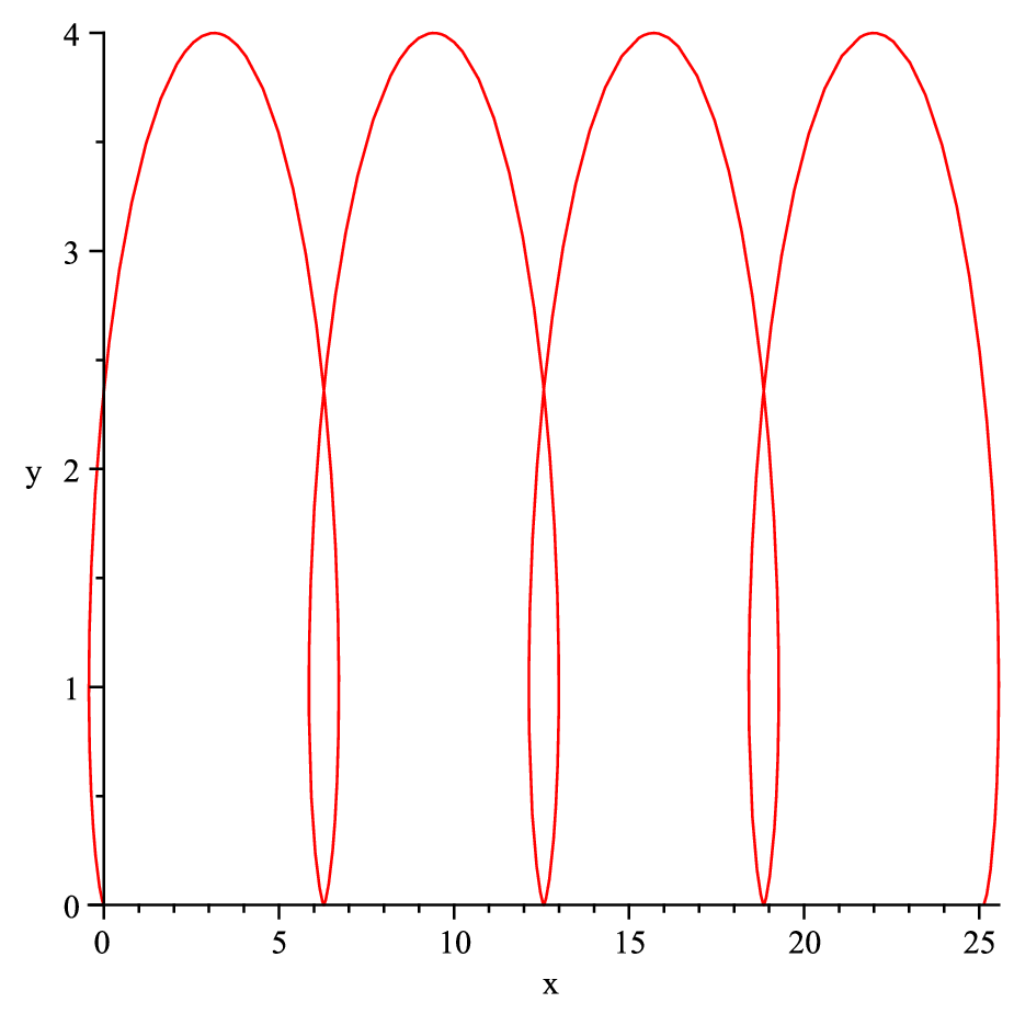

The particular initial conditions (38) have been chosen because they are easy to realize in a qualitative home experiment. The first step consists in creating a gently inclined plane with the help of two books. Use a finger of one hand to keep the coin upright, with its plane perpendicular to the slightly slanting edge of the inclined plane. Then release the coin at the same time as you flick its rim with a finger of the other hand, as in Fig. 3. Qualitatively, the motion of the coin’s center of mass resembles the ones shown in Fig. 2, although a few trials may be needed to produce such a motion because the coin should be rolling without slipping from the start. One feature that is unequivocally borne out by this domestic experiment is that the coin does not fall all the way down, but reverses its downward motion and climbs back up the inclined plane, in violation of what intuition suggests. This behavior, which is also displayed by a skate Flannery3, is sometimes regarded as paradoxical Arnold, and invoked to suggest that nonholonomic mechanics leads to unphysical behavior. The paradox seems to come from the fact that nonholonomic dynamics predicts that “…on the average the skate does not slide off from the inclined plane”. For this reason, so the argument goes, one would be justified in studying vakonomic mechanics as a viable competitor to nonholonomic mechanics. Accordingly, it has been suggested that the choice between vakonomic and nonholonomic mechanics in each concrete case can be answered only by experiment Arnold. As a matter of fact, it is vakonomic mechanics that gives rise to unphysical behavior for a skate on an inclined plane: for horizontal initial center-of-mass velocity and no initial rotation, in a neighborhood of the skate goes up the inclined plane Zampieri.
Rotational dynamics is full of surprises and rich in examples that violate our intuitive expectations, cases in point being the tippe top Cohen, the spinning cylinder Jackson, the asymmetric top Mecholsky and the rattleback Jones. Intuition may fail even in elementary rigid body dynamics Lemos3. Although the motion predicted by nonholonomic mechanics for the coin’s center of mass is counterintuitive, it is actually realized in Nature.

IV.2 Rolling coin dynamics according to vakonomic mechanics
From the Lagrangian (24) and the constraint functions (26) it follows that the vakonomic equations of motion (17) become
| (41) | |||||
| (42) | |||||
| (43) | |||||
| (44) |
These equations of motion differ in substantial aspects from the nonholonomic equations of motion. The most striking discrepancy is between equations (44) and (30).
IV.3 Complete inequivalence of vakonomic and nonholonomic mechanics
The following is the main result of this paper.
Proposition.
Except for the trivial case , in which the constraints (25) are actually holonomic, vakonomic mechanics is completely inequivalent to nonholonomic mechanics for the rolling coin on an inclined plane.
Proof.
Our purpose is to prove that equations (41)-(44) do not possess solutions of the form (31), (35), (36) and (37) no matter what the values of and may be. We start by noting that equation (41) leads to
| (45) |
Similarly, from equation (42) we get
| (46) |
Since from (31), equation (44) yields
| (47) |
where the constraints (25) have been used. Insertion of (45) and (46) into (47) leads to
| (48) |
Suppose , so that . Consider the sequence defined by where . The sequence is such that as according as or . Equations (36) and (37) give
| (49) |
With these results, equation (48) evaluated at reduces to
| (50) |
Since the left-hand side of this equation is a constant whereas its right-hand side tends to plus infinity as , equation (48) cannot be satisfied whatever the values of and may be. ∎
Remark. If , the expression within brackets on the right-hand side of (48) no longer contains a term proportional to . As a consequence, equation (48) can be satisfied by the choices and , in agreement with the results in Cortes1 and Fernandez regarding the rolling coin on a horizontal plane.
Finally, it is to be noted that, for a ball rolling without slipping on a rotating table, Lewis and Murray Lewis showed that for some particular initial conditions the nonholonomic motion is not vakonomic. Here, for the rolling coin on an inclined plane, we have proved that for all nontrivial initial conditions the nonholonomic motion is inaccessible from vakonomic mechanics.
V Conclusions
The proposal of vakonomic mechanics as a viable model to describe the dynamics of nonholonomic systems is fraught with predicaments.
From a theoretical point of view, the presence of both and in the equations of motion of vakonomic mechanics means that in order to determine the motion uniquely one has to specify , the values of the Lagrange multipliers at the initial instant . This implies that the well-tested Newtonian mechanics would have to be replaced by a new mechanics containing hidden variables, whose physical meaning is mysterious. Moreover, this entails, given that the Lagrange multipliers are directly connected to the constraint forces, that the initial accelerations would have to be prescribed together with the initial positions and velocities, which by all available evidence is not physically sound. Hidden-variable quantum theories are not successful as alternatives to quantum mechanics, but the lattter’s probabilistic nature justifies the attempts to build them. Since macroscopic physics is deterministic, there does not appear to be a corresponding motivation to search for hidden variables in classical mechanics. Thus, it seems fair to say that the physical significance of vakonomic mechanics, if any, remains opaque Kharlamov; Flannery2; Flannery3.
As to the actual behavior of nonholonomic systems, experimental studies Lewis; Kai favor (8) as the correct equations of motion. The qualitave home experiment described in the present paper corroborates these findings.
If, as held by advocates of vakonomic mechanics Arnold, experiment alone can decide between vakonomic and nonholonomic mechanics in each concrete case, experiment has been speaking loudly for nonholonomic mechanics and against vakonomic mechanics.
References
- (1) M. de León, “A historical review on nonholomic mechanics,” Revista de la Real Academia de Ciencias Exactas, Fisicas y Naturales. Serie A. Matematicas 106, 191–224 (2012).
- (2) A. V. Borisov, I. S. Mamaev and I. A. Bizyaev, “Historical and critical review of the development of nonholonomic mechanics: the classical period,” Regul. Chaotic Dyn. 21, 455–476 (2016).
- (3) H. Hertz, Die Prinzipen der Mechanick in Neuen Zusammenhange dargestellt (Leipzig, 1894). English translation: H. Hertz, The Principles of Mechanics Presented in a New Form (Dover, New York, 1944).
- (4) N. A. Lemos, Analytical Mechanics (Cambridge University Press, Cambridge, 2018).
- (5) L.-S. Wang and Y.-H. Pao, “Jourdain’s variational equation and Appell’s equation of motion for nonholonomic dynamical systems,” Am. J. Phys. 71, 72-82 (2003).
- (6) Ju. I. Neĭmark and N. A. Fufaev, Dynamics of Nonholonomic Systems (American Mathematical Society, Providence, RI, 1972).
- (7) J. Janová and J. Musilová, “The streetboard rider: an appealing problem in non-holonomic mechanics,” Eur. J. Phys. 31, 333–345 (2010).
- (8) B. d’Andréa-Novel, G. Campion and G. Bastin, “Control of nonholonomic wheeled mobile robots by state feedback linearization,” International Journal of Robotics Research 14, 543-599 (1995).
- (9) E. J. Rodríguez-Seda, C. Tang, M. W. Spong and D. M. Stipanović, “Trajectory tracking with collision avoidance for nonholonomic vehicles with acceleration constraints and limited sensing,” International Journal of Robotics Research 33, 1569-1592 (2014).
- (10) V. V. Kozlov, “Dynamics of systems with nonintegrable constraints. I-III,” Mosc. Univ. Mech. Bull. 37, 27-34 (1982); 37, 74-80 (1982); 38, 40-51 (1983).
- (11) V. V. Kozlov, “Realization of nonintegrable constraints in classical mechanics,” Sov. Phys. Dokl. 28, 735-737 (1983).
- (12) V. I. Arnold, V. V. Kozlov and A. I. Neishtadt, Mathematical Aspects of Classical and Celestial Mechanics, 3rd ed. (Springer, Berlin, 2006).
- (13) G. A. Bliss, “The problem of Lagrange in the calculus of variations,” Amer. J. Math. 52, 673-744 (1930).
- (14) G. A. Bliss, Lectures on the Calculus of Variations (University of Chicago Press, Chicago, 1946).
- (15) F. Cardin and M. Favretti, “On nonholonomic and vakonomic dynamics of mechanical systems with nonintegrable constraints,” J. Geom. Phys. 18, 295-325 (1996).
- (16) A. V. Borisov, I. S. Mamaev and I. A. Bizyaev, “Dynamical systems with non-integrable constraints, vakonomic mechanics, sub-Riemannian geometry, and non-holonomic mechanics,” Russ. Math. Surv. 72, 783-840 (2017).
- (17) J. Cortés, M. de León, D. M. de Diego and S. Martínez, “Geometric description of vakonomic and nonholonomic dynamics. Comparison of solutions”, SIAM J. Control Optim. 41, 1389–1412 (2003). arXiv:math/0006183v1 [math.DG].
- (18) S. Martínez, J. Cortés and M. de León, “The geometrical theory of constraints applied to the dynamics of vakonomic mechanical systems: The vakonomic bracket,” J. Math. Phys. 41, 2090-2120 (2000).
- (19) J. Llibre, R. Ramírez and N. Sadovskaia, “A new approach to the vakonomic mechanics,” Nonlinear Dynam. 78, 2219-2247 (2014).
- (20) J. Koiller, “Reduction of Some Classical Non-Holonomic Systems with Symmetry,” Arch. Rational Mech. Anal. 118, 113-148 (1992).
- (21) M. Favretti, “Equivalence of Dynamics for Nonholonomic Systems with Transverse Constraints,” J. Dyn. Differ. Equ. 10, 511-535 (1998).
- (22) O. E. Fernandez and A. M. Bloch, “Equivalence of the dynamics of nonholonomic and variational nonholonomic systems for certain initial data,” J. Phys. A: Math. Theor. 41, 344005 (2008).
- (23) P. V. Kharlamov, “A critique of some mathematical models of mechanical systems with differential constraints,” J. Appl. Math. Mech. 56, 584-594 (1992).
- (24) S.-M. Li and J. Berarkdar, “On the validity of the vakonomic model and the Chetaev model for constraint dynamical systems,” Rep. Math. Phys. 60, 107-116 (2007).
- (25) G. Zampieri, “Nonholonomic versus vakonomic dynamics,” J. Diff. Equ. 163, 335-347 (2000). arXiv:1204.3387v2 [math.DS].
- (26) A. D. Lewis and R. M. Murray, “Variational principles for constrained systems: Theory and experiment,” Int. J. Non-Linear Mechanics 30, 793-815 (1995).
- (27) T. Kai, “Experimental comparison between nonholonomic and vakonomic mechanics in nonlinear constrained systems,” Nonlinear Theory and Its Applications 4, 482-499 (2013).
- (28) L. A. Pars, A Treatise on Analytical Dynamics (Heinemann, London, 1965).
- (29) H. Goldstein, C. P. Poole, Jr. and J. L. Safko, Classical Mechanics, 3rd ed. (Addison Wesley, San Francisco, 2001).
- (30) E. T. Whittaker, A Treatise on the Analytical Dynamics of Particles and Rigid Bodies, 4th ed. (Cambridge University Press, Cambridge, 1937).
- (31) N. A. Lemos and M. Moriconi, “On the consistency of the Lagrange multiplier method in classical mechanics,” arXiv:2012.11059v1 [physics.class-ph].
- (32) H. Rund, The Hamilton-Jacobi Theory in the Calculus of Variations (Van Nostrand, London, 1966).
- (33) E. J. Saletan and A. H. Cromer, “A variational principle for nonholonomic systems,” Am. J. Phys. 38, 892-897 (1970).
- (34) M. R. Flannery, “d’Alembert–Lagrange analytical dynamics for nonholonomic systems,” J. Math. Phys. 52, 032705 (2011).
- (35) J. R. Ray, “Nonholonomic Constraints,” Am. J. Phys. 34, 406–408 (1966).
- (36) G. H. Goedecke, “Undetermined multiplier treatments of the Lagrange problem,” Am. J. Phys. 34, 571–574 (1966).
- (37) J. R. Ray, “Erratum: Nonholonomic Constraints [Am. J. Phys. 34, 406 (1966)],” Am. J. Phys. 34, 1202–1203 (1966).
- (38) http://astro.physics.sc.edu/Goldstein/1-2-3To6.html.
- (39) A. C. B. Antunes, C. Sigaud, and P. C. G. de Moraes, “Controlling nonholonomic Chaplygin systems,” Braz. J. Phys. 40, 131-140 (2010).
- (40) R. J. Cohen, “The tippe top revisited,” Am. J. Phys. 45, 12-17 (1977). https://www.youtube.com/watch?v=PysvuvuWUKo.
- (41) D. P. Jackson, J. Huddy, Adam Baldoni and William Boyes, “The mysterious spinning cylinder – Rigid-body motion that is full of surprises,” Am. J. Phys. 87, 85-94 (2019). https://www.youtube.com/watch?v=wQTVcaA3PQw.
- (42) N. A. Mecholsky, “Analytic formula for the geometric phase of an asymmetric top,” Am. J. Phys. 87, 245-254 (2019). https://www.youtube.com/watch?v=1n-HMSCDYtM.
- (43) S. Jones and H. E. M. Hunt, “Rattlebacks for the rest of us,” Am. J. Phys. 87, 699-713 (2019). https://www.youtube.com/watch?v=6zagApUMj3c.
- (44) N. A. Lemos, “Failure of intuition in elementary rigid body dynamics,” Eur. J. Phys. 29, N1 (2008).
- (45) M. R. Flannery, “The elusive d’Alembert-Lagrange dynamics of nonholonomic systems,” Am. J. Phys. 79, 932-944 (2011).