跳到论文正文
W Papers独立论文阅读器 arXiv:2105.02094 论文正文 计算阅读时间 · 0%
引用这篇论文根据当前论文元数据生成,正式投稿前建议核对。


License: CC BY 4.0
arXiv:2105.02094v1 [econ.TH] 05 May 2021

Sustainability of collusion and market transparency in a sequential search market: a generalization

Jacopo De Tullio*    Giuseppe Puleio** Affiliation: * Department of Decision Sciences, Bocconi University, Italy Affiliation: ** Department of Finance, Bocconi University, Italy
May 2021
Abstract

The present work generalizes the analytical results of Petrikaite (2016) to a market where more than two firms interact. As a consequence, for a generic number of firms in the oligopoly model described by Janssen et al (2005), the relationship between the critical discount factor which sustains the monopoly collusive allocation and the share of perfectly informed buyers is non-monotonic, reaching a unique internal point of minimum. The first section locates the work within the proper economic framework. The second section hosts the analytical computations and the mathematical reasoning needed to derive the desired generalization, which mainly relies on the Leibniz rule for the differentiation under the integral sign and the Bounded Convergence Theorem.

1 Introduction

The work of Petrikaite (2016) analyses the sustainability of the monopoly collusive allocation as a Subgame Perfect Equilibrium (SPE) of the super-game extension of the model of costly sequential search described by Janssen et al (2005)11 1 We refer to the case of full consumer participation addressed by Janssen et al (2005). Within this framework, this model should be thought of as the inelastic demand version of the seminal model of Stahl (1989). in the case of a duopoly. A well established result of the theory of industrial organization asserts that in a infinitely repeated oligopoly game with almost perfect monitoring the monopoly collusive allocation constitutes a SPE provided that the inter-temporal discount factor δ∈(0,1)\delta\in(0,1) is not inferior than a certain critical value.22 2 That is, the factor through which firms, at time tt, discount expected profits which will mature at time t+1t+1. Indeed, if firms are sufficiently patient, they are willing to renounce to the short term gains that they could achieve best-responding against the collusive agreement, in order to preserve the future supracompetitive margins that collusion is expected to bring about. This is the classic model of tacit collusion when firms play grim-trigger strategies. See, inter alia, Motta (2004) and Tirole (1988). The minimum discount factor δ∗\delta^{*} is related to the one-shot Nash Equilibrium profits π∗\pi^{*}, the collusive profits πc\pi^{c} and the deviation profits πd\pi^{d} by the following equation:

δ∗=πd−πcπd−π∗∈(0,1)\delta^{*}=\frac{\pi^{d}-\pi^{c}}{\pi^{d}-\pi^{*}}\in(0,1)

In the model of Janssen et al (2005), consumers search sequentially in a homogeneous market with perfect recall; a portion λ\lambda of them can become aware of all the different quotations listed by the firms at no cost, while the remaining part of buyers suffer a constant search cost ss, smaller than their maximum willingness to pay vv, for each price they might desire to observe, except for the first one. Demand is inelastic: each consumer purchases one unit of output, as long as the minimum price of which she is aware does not exceed her maximum willingness to pay. Given this environment, in a monopoly collusive allocation it holds that πc=vN\pi^{c}=\frac{v}{N}, πd=v⁡(1−λN+λ)\pi^{d}=v(\frac{1-\lambda}{N}+\lambda) and π∗=p∗​(1−λ)N\pi^{*}=\frac{p^{*}(1-\lambda)}{N} where NN represents the number of firms in the market and

p∗=s1−∫01d​y1+λ1−λ​N​yN−1=s1−G⁡(λ,N)p^{\ast}=\frac{s}{1-\int_{0}^{1}\frac{dy}{1+\frac{\lambda}{1-\lambda}Ny^{N-1}}}=\frac{s}{1-G(\lambda;N)}

represents the endogenous reservation price, which is defined as the price that makes imperfectly informed buyers indifferent between purchasing at the price at hand or carrying out a further search through the market. NN, λ\lambda, vv and ss are all exogenous, and it is assumed that 0<s<v0<s<v and 1>λ≥λ^1>\lambda\geq{\hat{\lambda}}, so that a reservation price equilibrium is achieved33 3 A reservation price equilibrium exists if and only if λ≥λ^\lambda\geq{\hat{\lambda}} where λ^\hat{\lambda} satisfies 1−∫01d​y1+λ^1−λ^​N​yN−1=sv1-\int_{0}^{1}\frac{dy}{1+\frac{\hat{\lambda}}{1-\hat{\lambda}}Ny^{N-1}}=\frac{s}{v}, given s∈(0,v)s\in(0,v). The reservation price will correspond to the upper bound of the prices distribution; see Pennerstorfer et al (2016) and Janssen et al (2005) for more details. The case of a no-reservation price equilibrium is significantly less interesting, since in that case the critical discount factor will depend only on the number of firms in the market, being insensitive to variations in the relative number of perfectly informed buyers. , while y∈[0,1]y\in[0,1] is an auxiliary variable derived from the equilibrium distribution of prices.
In the light of what has been specified above, it is possible to write:

δ∗=λ⁡(N−1)1+λ⁡(N−1)−p∗​(1−λ)v\delta^{\ast}=\frac{\lambda\left(N-1\right)}{1+\lambda\left(N-1\right)-\frac{p^{\ast}\left(1-\lambda\right)}{v}} (1)

and

∂δ∗∂λ=1(πd−π∗)2​[∂π∗∂λ​(πd−πc)+∂πd∂λ​(πc−π∗)]==1(πd−π∗)2​[vN2​(N−1)​(v−p∗+∂p∗∂λ​(1−λ)​λ)]\begin{split}\frac{\partial{\delta^{\ast}}}{\partial\lambda}=\frac{1}{\left(\pi^{d}-\pi^{\ast}\right)^{2}}\left[\frac{\partial\pi^{\ast}}{\partial\lambda}\left(\pi^{d}-\pi^{c}\right)+\frac{\partial\pi^{d}}{\partial\lambda}\left(\pi^{c}-\pi^{\ast}\right)\right]=\\ =\frac{1}{\left(\pi^{d}-\pi^{\ast}\right)^{2}}\left[\frac{v}{N^{2}}\left(N-1\right)\left(v-p^{\ast}+\frac{\partial p^{\ast}}{\partial\lambda}\left(1-\lambda\right)\lambda\right)\right]\end{split}

Let

Γ⁡(λ,N)=v−p∗+∂p∗∂λ​(1−λ)​λ\mathrm{\Gamma}\left(\lambda;N\right)=v-p^{\ast}+\frac{\partial p^{\ast}}{\partial\lambda}\left(1-\lambda\right)\lambda

Petrikaite (2016) shows that ∂Γ⁡(λ,2)∂λ|λ∈(0,1)>0\frac{\partial\Gamma\left(\lambda;2\right)}{\partial\lambda}|_{\ \lambda\ \in\left(0,1\right)}>0; a fortiori, ∂Γ⁡(λ,2)∂λ|λ∈(λ^,1)>0\frac{\partial\Gamma\left(\lambda;2\right)}{\partial\lambda}|_{\lambda\ \in\left(\hat{\lambda},1\right)}>0. As limλ→λ^Γ⁡(λ,2)=v2​(1v−2​λ^(1+λ^)​s)<0\lim_{\lambda\to\hat{\lambda}}{\mathrm{\Gamma}\left(\lambda;2\right)}=v^{2}\left(\frac{1}{v}-\frac{2\hat{\lambda}}{\left(1+\hat{\lambda}\right)s}\right)<0 and limλ→1Γ⁡(λ,2)=v−s>0\lim_{\lambda\to 1}{\mathrm{\Gamma}\left(\lambda;2\right)}=v-s>0, it is possible to deduce that, given N=2N=2 and s∈(0,v)s\in(0,v), ∃λ~\exists\ \widetilde{\lambda} such that ∀λ∈(λ^,λ~]\forall\ \lambda\in\ (\hat{\lambda},\widetilde{\lambda}] ∂δ∗∂λ≤0\frac{\ \partial\delta^{\ast}}{\partial\lambda}\ \leq 0 and ∀λ∈(λ~,1)\forall\ \lambda\in\ \left(\widetilde{\lambda},1\right) ∂δ∗∂λ>0\frac{\ \partial\delta^{\ast}}{\partial\lambda}>0.

2 The general case

The aim of this section is to show that the results which apply to a duopoly can be extended to a case where a higher number of firms interact: provided that the share of shoppers is sufficiently high so that a reservation price equilibrium is achieved, the critical discount factor will be first decreasing and later increasing in this parameter, reaching a unique internal point of minimum. Hence, in what follows, N>2N>2 (N∈ℕN\in\mathbb{N})44 4 Clearly, from an economic point of view, it is reasonable to restrict ourselves to N≤10N\leq 10..

2.1 Deriving the inequality

Consider again

Γ⁡(λ,N)=v−p∗+∂p∗∂λ​(1−λ)​λ=\mathrm{\Gamma}\left(\lambda;N\right)=v-p^{\ast}+\frac{\partial p^{\ast}}{\partial\lambda}\left(1-\lambda\right)\lambda= (2)
=v−p∗−(1−λ)​λ​(p∗1−G⁡(λ,N)⋅∫01N​yN−1((1−λ)+λ​N​yN−1)2​𝑑y)=v-p^{\ast}-\left(1-\lambda\right)\lambda\left(\frac{p^{\ast}}{1-G\left(\lambda;N\right)}\cdot\ \int_{0}^{1}{\frac{Ny^{N-1}}{\left(\left(1-\lambda\right)+\lambda Ny^{N-1}\right)^{2}}dy}\right)

Notice that

∫01N​yN−1((1−λ)+λ​N​yN−1)2​𝑑y=1(1−λ)2​∫01N​yN−2​y(1+λ(1−λ)​N​yN−1)2​𝑑y=\int_{0}^{1}{\frac{Ny^{N-1}}{\left(\left(1-\lambda\right)+\lambda Ny^{N-1}\right)^{2}}dy}=\frac{1}{\left(1-\lambda\right)^{2}}\int_{0}^{1}{\frac{Ny^{N-2}y}{\left(1+\frac{\lambda}{\left(1-\lambda\right)}Ny^{N-1}\right)^{2}}dy=}
=1λ⁡(N−1)​[G⁡(λ,N)​(1+λ⁡(N−1))−(1−λ)(1+λ⁡(N−1))​(1−λ)]>0=\frac{1}{\lambda\left(N-1\right)}\left[\frac{G\left(\lambda;N\right)\left(1+\lambda\left(N-1\right)\right)-\left(1-\lambda\right)}{\left(1+\lambda\left(N-1\right)\right)\left(1-\lambda\right)}\right]>0

So, equation (2) can be rewritten as

Γ⁡(λ,N)=v−p∗​{1+(G⁡(λ,N)​(1+λ⁡(N−1))−(1−λ)(N−1)​(1+λ⁡(N−1))​(1−G⁡(λ,N)))}=\mathrm{\Gamma}\left(\lambda;N\right)=v-p^{\ast}\left\{1+\left(\frac{G\left(\lambda;N\right)\left(1+\lambda\left(N-1\right)\right)-\left(1-\lambda\right)}{\left(N-1\right)\left(1+\lambda\left(N-1\right)\right)\left(1-G\left(\lambda;N\right)\right)}\right)\right\}=
=v−p∗​{1+H⁡(λ)}=v-p^{\ast}\left\{1+H(\lambda)\right\}

Given that limλ→λ^Γ⁡(λ,N)=v−v⁡{1+H⁡(λ^)}<0\lim_{\lambda\to\hat{\lambda}}{\mathrm{\Gamma}\left(\lambda;N\right)}=v-v\left\{1+H(\hat{\lambda})\right\}<0 and limλ→1Γ⁡(λ,N)=v−s>0\lim_{\lambda\to 1}{\mathrm{\Gamma}\left(\lambda;N\right)}=v-s>0, in order to show that equation (1) has a unique internal point of minimum it is sufficient to show that

∂Γ⁡(λ,N)∂λ=−[∂p∗∂λ​{1+H⁡(λ)}+p∗​∂H⁡(λ)∂λ]>0∀λ∈(λ^,1)\frac{\partial\Gamma\left(\lambda;N\right)}{\partial\lambda}=-\left[\frac{\partial p^{\ast}}{\partial\lambda}\left\{1+H(\lambda)\right\}+p^{\ast}\frac{\partial H(\lambda)}{\partial\lambda}\right]>0\hskip 14.22636pt\forall\hskip 2.84544pt\lambda\in(\hat{\lambda},1) (3)

As ∂p∗∂λ<0\frac{\partial p^{\ast}}{\partial\lambda}<0 ∀\forall λ∈(λ^,1)\lambda\in(\hat{\lambda},1) and the reservation price is clearly positive, to show that equation (3) holds it is sufficient to show that ∂H⁡(λ)∂λ<0\frac{\partial H(\lambda)}{\partial\lambda}<0 ∀\forall λ∈(0,1)\lambda\in(0,1).
Algebraic manipulations reveal that

(N−1)2​(1+λ⁡(N−1))2​(1−G⁡(λ,N))2N2⋅∂H⁡(λ)∂λ=(1−G⁡(λ,N)(1−λ))\frac{\left(N-1\right)^{2}\left(1+\lambda\left(N-1\right)\right)^{2}\left(1-G\left(\lambda;N\right)\right)^{2}}{N^{2}}\cdot\frac{\partial H(\lambda)}{\partial\lambda}=\left(1-\frac{G\left(\lambda;N\right)}{\left(1-\lambda\right)}\right)

So that the condition G⁡(λ,N)≥1−λG\left(\lambda;N\right)\geq{1-\lambda} ∀\forall λ∈(0,1)\lambda\in(0,1) is sufficient to show that equation (3) indeed holds.

2.2 Solving the inequality

Our ultimate objective is, therefore, to show that:

G⁡(λ,N)−(1−λ)≥0​∀λ∈(0,1),∀N>2∈ℕG\left(\lambda;N\right)-\left(1-\lambda\right)\geq 0\ \forall\ \lambda\ \in\ \left(0,1\right)\ ,\ \forall\ \ N>2\in\ \mathbb{N} (4)

To this end, it is necessary to exploit the Leibniz rule55 5 See Mukhopadhyay(2000). and the Bounded Convergence Theorem for the Riemann integral66 6 See Gordon(2000).. These two results allow us to state that limλ→0G′​(λ,N)=−1\lim_{\lambda\to 0}{G^{\prime}\left(\lambda;N\right)=-1}, limλ→0G′′​(λ,N)>0\lim_{\lambda\to 0}{G^{\prime\prime}\left(\lambda;N\right)>0} and ∂G′′​(λ,N)∂λ<0\frac{\partial G^{\prime\prime}\left(\lambda;N\right)}{\partial\lambda}<0 ∀\forall λ∈(0,1)\lambda\in(0,1). Importantly, it has been already established that limλ→0G⁡(λ,N)=1\lim_{\lambda\to 0}{G\left(\lambda;N\right)=1} and limλ→1G⁡(λ,N)=0\lim_{\lambda\to 1}{G\left(\lambda;N\right)=0}77 7 See Janssen et al (2005) in this regard..
Let us show first that limλ→0G′​(λ,N)=−1\lim_{\lambda\to 0}{G^{\prime}\left(\lambda;N\right)=-1}, where, by the Leibniz rule,

G′(λ;N)=−∫01N​yN−1[(1+λ(NyN−1−1)]2dyG^{\prime}\left(\lambda;N\right)=-\int_{0}^{1}{\frac{Ny^{N-1}}{{[(1+\lambda(Ny^{N-1}-1)]}^{2}}dy}

It is useful to write

limλ→0∫01N​yN−1[(1+λ(NyN−1−1)]2​𝑑y=limn→∞∫01N​yN−1[(1+λn(NyN−1−1)]2​𝑑y\lim_{\lambda\to 0}{\int_{0}^{1}{\frac{Ny^{N-1}}{{[(1+\lambda(Ny^{N-1}-1)]}^{2}}dy}}=\lim_{n\to\infty}{\int_{0}^{1}{\frac{Ny^{N-1}}{{[(1+\lambda_{n}(Ny^{N-1}-1)]}^{2}}dy}}

where {λn}\{\lambda_{n}\} is a generic sequence which satisfies ∀\forall n∈ℕn\in\mathbb{N}, λn∈(0,1)\lambda_{n}\in(0,1) and limn→∞{λn}=0\lim_{n\to\infty}{\{\lambda_{n}\}}=0. Clearly, ∀\forall nn

fn​(y)=N​yN−1((1+λn​(N​yN−1−1))2CLOSEf_{n}(y)=\frac{Ny^{N-1}}{\left((1+\lambda_{n}(Ny^{N-1}-1)\right)^{2}}

is a Riemann-integrable function in [0,1][0,1]. Moreover, {fn​(y)}\left\{f_{n}(y)\right\} converges pointwise to f⁡(y)=N​yN−1f(y)=Ny^{N-1} in [0,1][0,1], which is a Riemann-integrable function. Hence, to apply the Bounded Convergence Theorem, it remains to show that the sequence {fn​(y)}\left\{f_{n}(y)\right\} is uniformly bounded. This motivates the following proposition.

Proposition 1. The sequence {fn​(y)}\left\{f_{n}(y)\right\} is uniformly bounded.
Proof. The proof works by contradiction. Suppose ∃\exists n∗n^{*} such that ∄\nexists M∈ℝ+M\in\mathbb{R_{+}} which satisfies |fn∗​(y)|=fn∗​(y)≤M\left|f_{n^{*}}(y)\right|=f_{n^{*}}(y)\leq{M},∀\forall y∈[0,1]y\in[0,1]. Consider, for an arbitrary chosen ε∈(0,1)\varepsilon\in(0,1), the set AεA_{\varepsilon}={\{λn\lambda_{n} ∉\not\in Bε​(0)B_{\varepsilon}(0)}\}, where Bε​(0)B_{\varepsilon}(0) is a neighbourhood of 00 of radius ε\varepsilon. For any ε\varepsilon, the set AεA_{\varepsilon} is either empty or finite. Suppose it is empty, so that λn∗∈Bε​(0)\lambda_{n^{*}}\in B_{\varepsilon}(0). Then, ∀\forall y∈[0,1N1N−1]y\in[0,{\frac{1}{N}}^{\frac{1}{N-1}}], ∀\forall nn

fε​(y)=N​yN−1((1+ε⁡(N​yN−1−1))2CLOSE≥fn​(y)f_{\varepsilon}(y)=\frac{Ny^{N-1}}{\left((1+\varepsilon(Ny^{N-1}-1)\right)^{2}}\geq{f_{n}(y)}

While ∀\forall y∈[1N1N−1,1]y\in[{\frac{1}{N}}^{\frac{1}{N-1}},1], f⁡(y)=N​yN−1≥fn​(y)f(y)=Ny^{N-1}\geq{f_{n}(y)}, ∀\forall nn.
As a result, set M=max⁡{maxy∈[0,1N1N−1]⁡fε​(y),N}≥fn∗​(y)M=\max{\{\max_{y\in[0,{\frac{1}{N}}^{\frac{1}{N-1}}]}{f_{\varepsilon}(y)},N\}}\geq{f_{n^{*}}(y)} and the desired contradiction is reached.
Let AεA_{\varepsilon} be finite. Then, ∃\exists λm=max⁡λn∈Aε\lambda_{m}=\max{\lambda_{n}\in A_{\varepsilon}}. Then, define

K=maxy∈[0,1N1N−1]⁡fλm​(y)K=\max_{y\in[0,{\frac{1}{N}}^{\frac{1}{N-1}}]}{f_{\lambda_{m}}(y)}

Setting M=max⁡{K,N}M=\max\{{K,N}\} we reach the desired contradiction, independently from whether λn∗∈Aε\lambda_{n^{*}}\in A_{\varepsilon} or not. The existence of the upper bound relies on the continuity of the functions fε​(y)f_{\varepsilon}(y) and fλm​(y)f_{\lambda_{m}}(y), which are defined on a compact interval. ■\blacksquare

As a consequence, from the Bounded Convergence Theorem:

limn→∞∫01N​yN−1[(1+λn(NyN−1−1)]2​𝑑y=∫01N​yN−1​𝑑y=1\lim_{n\to\infty}{\int_{0}^{1}{\frac{Ny^{N-1}}{{[(1+\lambda_{n}(Ny^{N-1}-1)]}^{2}}dy}}=\int_{0}^{1}{Ny^{N-1}dy}=1

and limλ→0G′​(λ,N)=−1\lim_{\lambda\to 0}{G^{\prime}(\lambda;N)}=-1.
Let us show the results for G′′​(λ,N)G^{\prime\prime}(\lambda;N). Given NN and yy, fN,y​(λ)=N​yN−1((1+λ⁡(N​yN−1−1))2CLOSEf_{N,y}(\lambda)=\frac{Ny^{N-1}}{\left((1+\lambda(Ny^{N-1}-1)\right)^{2}} is differentiable for λ\lambda in (0,1)(0,1). Thanks to this observation, it is licit to apply the Leibniz Rule, concluding that:

G′′​(λ,N)=∫012​N​yN−1​(N​yN−1−1)(1+λ​(N​yN−1−1)3CLOSE​𝑑yG^{\prime\prime}(\lambda;N)=\int_{0}^{1}{\frac{2Ny^{N-1}(Ny^{N-1}-1)}{{(1+\lambda(Ny^{N-1}-1)}^{3}}dy}

To evaluate limλ→0G′′​(λ,N)\lim_{\lambda\to 0}{G^{\prime\prime}(\lambda;N)}, define the sequence, for a given NN, {gn}\{g_{n}\}, with generic element

gn​(y)=2​N​yN−1​(N​yN−1−1)(1+λn​(N​yN−1−1))3g_{n}(y)=\frac{2Ny^{N-1}(Ny^{N-1}-1)}{{(1+\lambda_{n}(Ny^{N-1}-1))}^{3}}

where {λn}\{\lambda_{n}\} is a generic sequence which satisfies ∀\forall n∈ℕn\in\mathbb{N}, λn∈(0,1)\lambda_{n}\in(0,1) and limn→∞{λn}=0\lim_{n\to\infty}{\{\lambda_{n}\}}=0. We have that {gn}\{g_{n}\} is a sequence of Riemann integrable functions, since every gng_{n} is a continuous function defined on a compact interval. Moreover, the sequence converges pointwise to g⁡(y)=2​N​yN−1​(N​yN−1−1)g(y)=2Ny^{N-1}(Ny^{N-1}-1) in [0,1][0,1], which is a Riemann Integrable function. Uniform boundedness88 8 The proof is identical in spirit to the one of Proposition 1. of {gn}\{g_{n}\} ensures that the Bounded Convergence Theorem holds, so that we are allowed to write:

limn→∞∫012​N​yN−1​(N​yN−1−1)(1+λn​(N​yN−1−1))3​𝑑y=∫012​N​yN−1​(N​yN−1−1)​𝑑y=\lim_{n\to\infty}{\int_{0}^{1}{\frac{2Ny^{N-1}(Ny^{N-1}-1)}{{(1+\lambda_{n}(Ny^{N-1}-1)})^{3}}dy}}=\int_{0}^{1}{2Ny^{N-1}\left(Ny^{N-1}-1\right)dy}=
=2​N​(N2​(N−1)+1−1N)>0​∀N>2=2N\left(\frac{N}{2(N-1)+1}-\frac{1}{N}\right)>0\hskip 8.5359pt\forall\hskip 2.84544ptN>2

So that limλ→0G′′​(λ,N)>0\lim_{\lambda\to 0}{G^{\prime\prime}(\lambda;N)}>0. Finally, it is possible to notice that G′′​(λ,N)G^{\prime\prime}(\lambda;N) is strictly decreasing in λ∈(0,1)\lambda\in(0,1). For every given NN and every given yy, fN,y​(λ)=2​N​yN−1​(N​yN−1−1)(1+λ⁡(N​yN−1−1))3f_{N,y}(\lambda)=\frac{2Ny^{N-1}(Ny^{N-1}-1)}{{(1+\lambda(Ny^{N-1}-1))}^{3}} is differentiable in λ∈(0,1)\lambda\in(0,1). By the Leibniz Rule,

∂∂λ∫012​N​yN−1​(N​yN−1−1)(1+λ⁡(N​yN−1−1))3dy=∫01−6​N​yN−1​(N​yN−1−1)2(1+λ⁡(N​yN−1−1))4dy\frac{\partial}{\partial\lambda}\int_{0}^{1}{\frac{2Ny^{N-1}(Ny^{N-1}-1)}{{(1+\lambda(Ny^{N-1}-1))}^{3}}dy}=\int_{0}^{1}{-\frac{6Ny^{N-1}{(Ny^{N-1}-1)}^{2}}{{(1+\lambda(Ny^{N-1}-1))}^{4}}dy}

Given that

∫01N​yN−1​(N​yN−1−1)2(1+λ⁡(N​yN−1−1))4​𝑑y>∫01N​yN−1​(N​yN−1−1)2(1+λ⁡(N−1))4​𝑑y=\int_{0}^{1}{\frac{Ny^{N-1}{(Ny^{N-1}-1)}^{2}}{{(1+\lambda(Ny^{N-1}-1))}^{4}}dy>}\int_{0}^{1}{\frac{Ny^{N-1}{(Ny^{N-1}-1)}^{2}}{{(1+\lambda(N-1))}^{4}}dy}=
=1(1+λ⁡(N−1))4⋅{N33​(N−1)+1+1−2​N22​(N−1)+1}>0​∀N∈ℕ>2=\frac{1}{{(1+\lambda(N-1))}^{4}}\cdot\{\frac{N^{3}}{3(N-1)+1}+1-\frac{{2N}^{2}}{2(N-1)+1}\}>0\hskip 5.69046pt\forall\hskip 2.84544ptN\in\mathbb{N}>2

Then ∂∂λ​G′′​(λ,N)<0\frac{\partial}{\partial\lambda}G^{\prime\prime}(\lambda;N)<0 ∀\forall λ∈(0,1)\lambda\in(0,1). This results is crucial in motivating the following proposition.

Proposition 2.
∀\forall
N∈ℕ>2N\in\mathbb{N}>2, there exists a unique λNf∈(0,1)\lambda_{N}^{f}\in(0,1) such that G′′​(λNf,N)=0G^{\prime\prime}(\lambda_{N}^{f};N)=0.
Proof. Uniqueness stems directly from the strict and decreasing monotonicity of the function G′′​(λ,N)G^{\prime\prime}(\lambda;N). Suppose that the inflection point did not exist. Then, G′′​(λ,N)>0G^{\prime\prime}(\lambda;N)>0 ∀\forall λ∈(0,1)\lambda\in(0,1) and, as a consequence, G′​(λ,N)>−1G^{\prime}(\lambda;N)>-1 ∀\forall λ∈(0,1)\lambda\in(0,1). Given that limλ→0G⁡(λ,N)=1\lim_{\lambda\to 0}G(\lambda;N)=1, this would contradict the result of limλ→1G⁡(λ,N)=0\lim_{\lambda\to 1}G(\lambda;N)=0. ■\blacksquare
So far, we have showed that ∀\forall N∈ℕN\in\mathbb{N}, exists a unique λNf∈(0,1)\lambda_{N}^{f}\in\ \left(0,1\right) such that G′​(λ,N)>−1G^{\prime}\left(\lambda;N\right)>-1 ∀\forall λ∈(0,λNf]\lambda\in(0,\lambda_{N}^{f}] and the function G⁡(λ,N)G\left(\lambda;N\right) is strictly concave in (λNf,1)(\lambda_{N}^{f},1). This preliminary conditions allow us to show the desired inequality.

Proposition 3.

G⁡(λ,N)−(1−λ)≥0​∀λ∈(0,1),∀N>2∈ℕG(\lambda;N)-(1-\lambda)\geq 0\hskip 5.69046pt\forall\hskip 2.84544pt\lambda\in\ (0,1),\hskip 5.69046pt\forall\hskip 2.84544ptN>2\in\mathbb{N}

Proof. Suppose ∃\exists λ¯∈(0,λNf]\bar{\lambda}\in(0,\lambda_{N}^{f}] such that G⁡(λ¯,N)<(1−λ¯)G(\bar{\lambda};N)<(1-\bar{\lambda}); this would contradict the results of limλ→0G⁡(λ,N)=1\lim_{\lambda\to 0}{G(\lambda;N)}=1 and ∀\forall λ∈(0,λNf]​G′​(λ,N)>−1\lambda\in(0,\lambda_{N}^{f}]\ G^{\prime}(\lambda;N)>-1. Suppose ∃\exists λ^∈(λNf,1)\hat{\lambda}\in(\lambda_{N}^{f},1) such that G⁡(λ^,N)<(1−λ^)G(\hat{\lambda};N)<(1-\hat{\lambda}). Then, given that G⁡(λNf,N)>(1−λNf)G(\lambda_{N}^{f};N)>(1-\lambda_{N}^{f}) and G′′​(λ,N)<0G^{\prime\prime}(\lambda;N)<0 ∀\forall λ∈(λNf,1)\lambda\in(\lambda_{N}^{f},1), the condition limλ→1G⁡(λ,N)=0\lim_{\lambda\to 1}{G(\lambda;N)}=0 would be impossible to be satisfied. ■\blacksquare
Thanks to Proposition 3, we are allowed to state that, given N∈ℕN\in\mathbb{N} and s∈(0,v)s\in(0,v), ∃\exists λ~\widetilde{\lambda} such that ∀λ∈(λ^,λ~]\forall\ \lambda\in\ (\hat{\lambda},\widetilde{\lambda}] ∂δ∗∂λ≤0\frac{\ \partial\delta^{\ast}}{\partial\lambda}\ \leq 0 and ∀λ∈(λ~,1)\forall\ \lambda\in\ \left(\widetilde{\lambda},1\right) ∂δ∗∂λ>0\frac{\ \partial\delta^{\ast}}{\partial\lambda}>0.

References

Gordon, R. (2000): A Convergence Theorem for the Riemann Integral. Mathematics Magazine, 73(2), 141-147.
Janssen, M., Moraga-González, J.L. and Wildenbeest, M. (2005): Truly Costly Sequential Search and Oligopolistic Pricing, International Journal of Industrial Organization 23, 451-466.
Motta, M. (2004): Competition Policy: Theory and Practice, Cambridge University Press.
Mukhopadhyay, N. (2000): Probability and Statistical Inference, New York: Marcel Dekker.
Petrikaite, V. (2016): Collusion with Costly Consumer Search, International Journal of Industrial Organization vol. 44, pp. 1-10.

List of Figures
Refer to caption
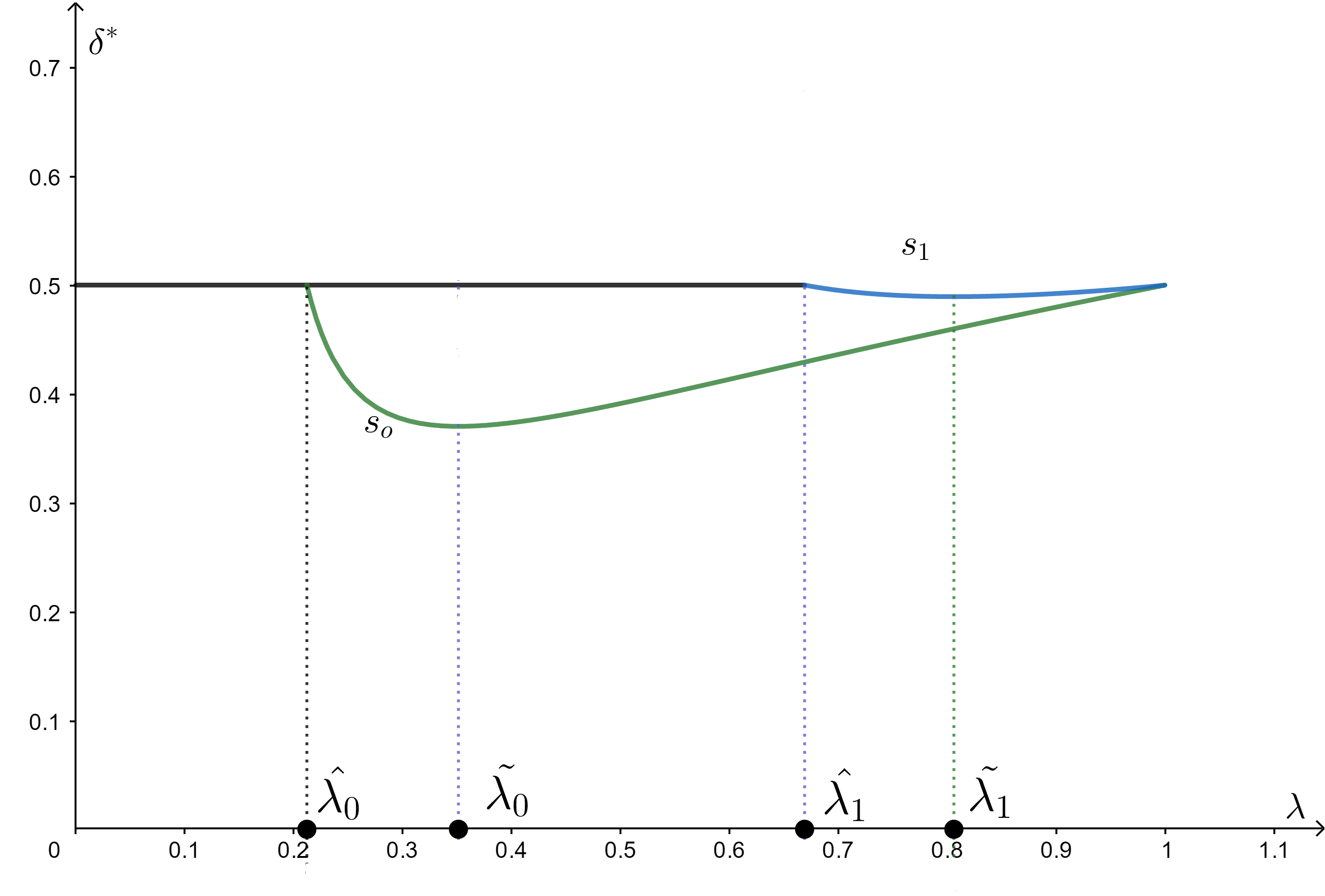
Figure 1: Critical discount factor as a function of the proportion of shoppers in a duopoly. Here, v=1v=1, s0=0.2s_{0}=0.2, s1=0.6s_{1}=0.6.
Refer to caption
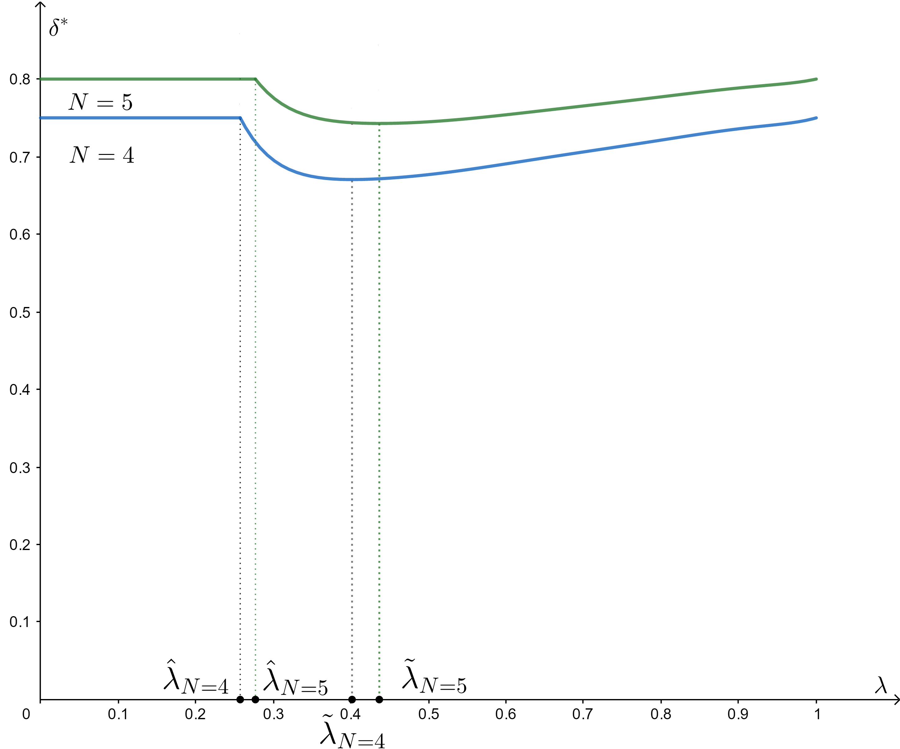
Figure 2: Critical discount factor as a function of the proportion of shoppers when N=4N=4 and N=5N=5. Here, v=1v=1 and s=0.2s=0.2 fixed. Numerical approximations show that the duopoly pattern is confirmed also when a higher number of firms interacts.
Refer to caption
Figure 3: Numerical approximations confirm the desired inequality. The black line indicates f⁡(λ)=1−λ≤G⁡(λ,3)≤G⁡(λ,4)≤G⁡(λ,5)f(\lambda)=1-\lambda\leq{G(\lambda;3)}\leq{G(\lambda;4)}\leq{G(\lambda;5)},where λ∈(0,1)\lambda\in(0,1).