New structures for colored HOMFLY-PT invariants

Shengmao Zhu Address: Department of Mathematics
Zhejiang International Studies University Address: Center of Mathematical Sciences
Zhejiang University
Hangzhou, 310027, China Email address: shengmaozhu@126.com, szhu@zju.edu.cn

Abstract.

In this paper, we present several new structures for the colored HOMFLY-PT invariants of framed links. First, we prove the strong integrality property for the normalized colored HOMFLY-PT invariants by purely using the HOMFLY-PT skein theory developed by H. Morton and his collaborators. By this strong integrality property, we immediately obtain several symmetric properties for the full colored HOMFLY-PT invariants of links. Then, we apply our results to refine the mathematical structures appearing in the Labastida-Mariño-Ooguri-Vafa (LMOV) integrality conjecture for framed links. As another application of the strong integrality, we obtain that the $q=1$ and $a=1$ specializations of the normalized colored HOMFLY-PT invariant are well-defined link polynomials. We find that a conjectural formula for the colored Alexander polynomial which is the $a=1$ specialization of the normalized colored HOMFLY-PT invariant implies that a special case of the LMOV conjecture for frame knot holds.

1. Introduction

1.1. Colored HOMFLY-PT invariants

Colored HOMFLY-PT invariant is an invariant of framed oriented links in $S^{3}$ whose components are colored with partitions. It can be viewed as a generalization of the HOMFLY-PT polynomial which was first discovered by Freyd-Yetter, Hoste, Lickorish-Millet, Ocneanu [25] and Przytycki-Traczyk [82]. Based on Turaev’s work [92], the HOMFLY-PT polynomial can be derived from the quantum group invariant labeled with the fundamental representation of the quantum group $U_{q}(sl_{N})$ . More generally, the colored HOMFLY-PT invariants can be constructed by using the quantum group invariants labeled with arbitrary irreducible representations of $U_{q}(sl_{N})$ which are labeled by partitions. We refer to [54, 58] for detailed definition of the colored HOMFLY-PT invariants along this way.

Historically, the quantum group approach to the colored HOMFLY-PT invariant originates from the $SU(N)$ Chern-Simons theory due to E. Witten [95]. The large $N$ duality between the $SU(N)$ Chern-Simons theory and topological string theory established in [96, 30, 79] makes the colored HOMFLY-PT invariant become a central object in geometry and physics. There have been spectacular developments on colored HOMFLY-PT invariant and its related topics over the years. For examples, the dependence of the colors is governed by recurrence relations which was proposed in [5], and proved in [28]. Moreover, these recurrence relations are conjectured to have deep relationships to the augmentation polynomials in knot contact homology [5, 4]. The relationship to the topological string theory connects the colored HOMFLY-PT invariants to Gromov-Witten theory [61, 49, 50, 18], Hilbert schemes [78], stable pair invariants [17, 62], quiver varieties [51, 42, 43, 81, 86, 87], knot contact homology [5, 4, 20, 24] etc. There also have being a lot of works devoted to the computations of the colored HOMFLY-PT invariants, see [58, 34, 76, 77, 27, 39, 97] and references therein.

On the other hand side, it is well-known that the HOMFLY-PT polynomial satisfies the fantastic skein relations which provide a combinatorial way to study them. From this point of view, Morton and his collaborators [67, 1, 2, 3, 63, 68, 31, 70, 71, 72] developed a systematic method, referred as HOMFLY-PT skein theory in this paper, to investigate the colored HOMFLY-PT invariants. The equivalence of the two approaches to colored HOMFLY-PT invariants via quantum group theory and HOMFLY-PT skein theory are presented in [1, 47], we also refer the reader to the appendix Section 8 for an explanation of this equivalence.

Comparing to the quantum group theory, HOMFLY-PT skein theory is more intuitional and straightforward. Therefore, in the paper, we mainly use the HOMFLY-PT skein theory as our tool to derive several new structures for colored HOMFLY-PT invariants.

1.1.1. Strong integrality

Let $\mathcal{L}$ be a framed oriented link with $L$ components $\mathcal{K}_{\alpha}$ for $\alpha=1,...,L$ ¹¹ 1 In the following, when we mention a link $\mathcal{L}$ , we always assume it is a framed oriented link with $L$ components given by $\mathcal{K}_{\alpha}$ for $\alpha=1,...,L$ ., given $\vec{\lambda}=(\lambda^{1},...,\lambda^{L})$ and $\vec{\mu}=(\mu^{1},...,\mu^{L})$ , where each $\lambda^{\alpha}$ (resp. $\mu^{\alpha}$ ) for $\alpha=1,..,L$ denotes a partition of a positive integer, the framed full colored HOMFLY-PT invariant of $\mathcal{L}$ colored by $[\vec{\lambda},\vec{\mu}]$ is given by

(1.1)

\displaystyle\mathcal{H}_{[\vec{\lambda},\vec{\mu}]}(\mathcal{L};q,a)=\mathcal{H}(\mathcal{L}\star\otimes_{\alpha=1}^{L}Q_{\lambda^{\alpha},\mu^{\alpha}}),

where $\mathcal{H}(\mathcal{L}\star\otimes_{\alpha=1}^{L}Q_{\lambda^{\alpha},\mu^{\alpha}})$ denotes the framed HOMFLY-PT polynomial of the link $\mathcal{L}$ decorated by $\otimes_{\alpha=1}^{L}Q_{\lambda^{\alpha},\mu^{\alpha}}$ , where each $Q_{\lambda^{\alpha},\mu^{\alpha}}$ denotes the skein basis element in the full skein $\mathcal{C}$ of the annulus, we recall their definitions in Section 2. In particular, when all the $\mu^{\alpha}$ is equal to the empty partition $\emptyset$ , we write $Q_{\lambda^{\alpha}}=Q_{\lambda^{\alpha},\mu^{\alpha}}$ for $\alpha=1,...,L$ , and denote $\mathcal{H}_{\vec{\lambda}}(\mathcal{L};q,a)=\mathcal{H}(\mathcal{L}\star\otimes_{\alpha=1}^{L}Q_{\lambda^{\alpha}})$ . Then we obtain the standard (framing independent) colored HOMFLY-PT invariant for $\mathcal{L}$ (e.g. the definitions in [58, 102])

(1.2)

\displaystyle W_{\vec{\lambda}}(\mathcal{L};q,a)=q^{-\sum_{\alpha=1}^{L}\kappa_{\lambda^{\alpha}}w(\mathcal{K}_{\alpha})}a^{-\sum_{\alpha=1}^{L}|\lambda^{\alpha}|w(\mathcal{K}_{\alpha})}\mathcal{H}_{\vec{\lambda}}(\mathcal{L};q,a).

When $\mathcal{L}$ has only one component, i.e. it is a knot which is usually denoted by $\mathcal{K}$ . We define the normalized framed full colored HOMFLY-PT invariants of $\mathcal{K}$ as follow

(1.3)

\displaystyle\mathcal{P}_{[\lambda,\mu]}(\mathcal{K};q,a)=\frac{\mathcal{H}_{[\lambda,\mu]}(\mathcal{K};q,a)}{\mathcal{H}_{[\lambda,\mu]}(U;q,a)}

where $U$ denotes the unknot throughout this paper. Then we have the following strong integrality property for $\mathcal{P}_{[\lambda,\mu]}(\mathcal{K};q,a)$ .

Theorem 1.1.

For any framed knot $\mathcal{K}$ , the normalized framed full colored HOMFLY-PT invariant satisfies

(1.4)

\displaystyle\mathcal{P}_{[\lambda,\mu]}(\mathcal{K};q,a)\in a^{\epsilon}\mathbb{Z}[q^{\pm 2},a^{\pm 2}].

where $\epsilon\in\{0,1\}$ is determined by the following formula

(1.5)

\displaystyle(|\lambda|+|\mu|)w(\mathcal{K})

\displaystyle\equiv\epsilon\mod 2.

where $w(\mathcal{K})$ is the writhe number of $\mathcal{K}$ .

In particular, the normalized colored HOMFLY-PT invariant $P_{\lambda}(\mathcal{K};q,a)$ of $\mathcal{K}$ , defined as $P_{\lambda}(\mathcal{K};q,a)=\frac{W_{\lambda}(\mathcal{K};q,a)}{W_{\lambda}(U;q,a)}$ , satisfies

(1.6)

\displaystyle P_{\lambda}(\mathcal{K};q,a)\in\mathbb{Z}[q^{2},a^{2}].

More generally, for a link $\mathcal{L}$ with $L$ components, one can define the $\alpha$ -normalized framed full colored HOMFLY-PT invariants for $\alpha=1,...,L$ as follow. We only decorate the $\alpha$ -component $\mathcal{K}_{\alpha}$ by $Q_{\lambda^{\alpha},\mu^{\alpha}}$ , and keep the other components invariant, we denote the corresponding colored HOMFLY-PT invariant of $\mathcal{L}$ by $\mathcal{H}_{[\lambda^{\alpha},\mu^{\alpha}]}(\mathcal{L};q,a)$ . Then the $\alpha$ -normalized colored framed full HOMFLY-PT invariant of $\mathcal{L}$ is given by

(1.7)

\displaystyle\mathcal{P}_{[\lambda^{\alpha},\mu^{\alpha}]}(\mathcal{L};q,a)=\frac{\mathcal{H}_{[\lambda^{\alpha},\mu^{\alpha}]}(\mathcal{L};q,a)}{\mathcal{H}_{[\lambda^{\alpha},\mu^{\alpha}]}(U;q,a)}.

We also have the following strong integrality theorem. 4.

Theorem 1.2.

For any framed link $\mathcal{L}$ with $L$ components $\mathcal{K}_{\alpha}$ for $\alpha=1,...,L$ , the $\alpha$ -normalized framed full colored HOMFLY-PT invariants satisfies

(1.8)

\displaystyle\mathcal{P}_{[\lambda^{\alpha},\mu^{\alpha}]}(\mathcal{L};q,a)\in a^{\epsilon}\mathbb{Z}[q^{\pm 2},a^{\pm 2}].

where $\epsilon\in\{0,1\}$ which is determined by the following formula

(1.9)

\displaystyle(|\lambda^{\alpha}|+|\mu^{\alpha}|)w(\mathcal{K}_{\alpha})+\sum_{\beta\neq\alpha}w(\mathcal{K}_{\beta})+L-1

\displaystyle\equiv\epsilon\mod 2.

As a consequence of Theorem 1.2, we have

Corollary 1.3.

For any framed link $\mathcal{L}$ , the framed full colored HOMFLY-PT invariants $\mathcal{H}_{[\vec{\lambda},\vec{\mu}]}(\mathcal{L};q,a)$ satisfies the following symmetric properties

(1.10)	$\displaystyle\mathcal{H}_{[\vec{\lambda},\vec{\mu}]}(\mathcal{L};-q,a)$	$\displaystyle=(-1)^{\sum_{\alpha=1}^{L}(\|\lambda^{\alpha}\|+\|\mu^{\alpha}\|)}\mathcal{H}_{[\vec{\lambda},\vec{\mu}]}(\mathcal{L};q,a)$
(1.11)	$\displaystyle\mathcal{H}_{[\vec{\lambda},\vec{\mu}]}(\mathcal{L};q,-a)$	$\displaystyle=(-1)^{\sum_{\alpha=1}^{L}(\|\lambda^{\alpha}\|+\|\mu^{\alpha}\|)(w(\mathcal{K}_{\alpha})+1)}\mathcal{H}_{[\vec{\lambda},\vec{\mu}]}(\mathcal{L};q,a)$
(1.12)	$\displaystyle\mathcal{H}_{[\vec{\lambda},\vec{\mu}]}(\mathcal{L};q^{-1},a)$	$\displaystyle=(-1)^{\sum_{\alpha=1}^{L}(\|\lambda^{\alpha}\|+\|\mu^{\alpha}\|)}\mathcal{H}_{[\vec{\lambda}^{\vee},\vec{\mu}^{\vee}]}(\mathcal{L};q,a).$

Remark 1.4.

We prove Theorem 1.1 and 1.2 by purely using HOMFLY-PT skein theory. It essentially uses all the crucial results developed by Morton and his collaborators. Comparing to our previous work [103], the proof presented here is essential and self-contained.

Remark 1.5.

From Corollary 1.3, one immediately obtain the following symmetries for colored HOMFLY-PT invariants $W_{\vec{\lambda}}(\mathcal{L};q,a)$ :

(1.13)	$\displaystyle W_{\vec{\lambda}}(\mathcal{L};-q,a)$	$\displaystyle=(-1)^{\sum_{\alpha=1}^{L}\|\lambda^{\alpha}\|}W_{\vec{\lambda}}(\mathcal{L};q,a),$
(1.14)	$\displaystyle W_{\vec{\lambda}}(\mathcal{L};q,-a)$	$\displaystyle=(-1)^{\sum_{\alpha=1}^{L}\|\lambda^{\alpha}\|}W_{\vec{\lambda}}(\mathcal{L};q,a),$
(1.15)	$\displaystyle W_{\vec{\lambda}}(\mathcal{L};q^{-1},a)$	$\displaystyle=(-1)^{\sum_{\alpha=1}^{L}\|\lambda^{\alpha}\|}W_{\vec{\lambda}^{\vee}}(\mathcal{L};q,a),$

which have appeared in previous literatures, see for example [57, 102].

1.1.2. Specializations

From Theorem 1.1, we obtain that the $q=1$ specialization of the normalized framed full colored HOMFLY-PT invariant $\mathcal{P}_{[\lambda,\mu]}(\mathcal{K};1,a)$ belongs to the ring $a^{\epsilon}\mathbb{Z}[a^{2}]$ . With a slight modification of the proof presented in [15], we obtain the formula

(1.16)

\displaystyle\mathcal{P}_{[\lambda,\mu]}(\mathcal{K};1,a)=\mathcal{P}(\mathcal{K};1,a)^{|\lambda|+|\mu|},

where $\mathcal{P}(\mathcal{K};q,a)=\frac{\mathcal{H}(\mathcal{K};q,a)}{\mathcal{H}(U;q,a)}$ is the normalized framed HOMFLY-PT polynomial.

We also consider the composite invariants studied in [60, 15] which is defined as follow. Given a link $\mathcal{L}$ with $L$ components and $\vec{\lambda},\vec{\mu},\vec{\nu}\in\mathcal{P}^{L}$ . Let $c_{\vec{\lambda},\vec{\mu}}^{\nu}=\prod_{\alpha=1}^{L}c_{\lambda^{\alpha},\mu^{\alpha}}^{\nu^{\alpha}}$ , where each $c_{\lambda^{\alpha},\mu^{\alpha}}^{\nu^{\alpha}}$ is the Littlewood-Richardson coefficient, then the framed composite invariant of $\mathcal{L}$ is defined by

(1.17)

\displaystyle\mathcal{C}_{\vec{\nu}}(\mathcal{L};q,a)=\sum_{\vec{\lambda},\vec{\mu}}c_{\vec{\lambda},\vec{\mu}}^{\vec{\nu}}\mathcal{H}_{[\vec{\lambda},\vec{\mu}]}(\mathcal{L};q,a).

In particular, for the knot $\mathcal{K}$ , we prove that the special framed composite invariant which is the following limit exists and satisfies the relation

(1.18)

\displaystyle\lim_{q\rightarrow 1}\frac{\mathcal{C}_{\nu}(\mathcal{K};q,a)}{\mathcal{C}_{\nu}(U;q,a)}=\mathcal{P}(\mathcal{K};1,a)^{|\nu|}.

On the other hand side, one can also consider the $a=1$ specialization of the normalized framed full colored HOMFLY-PT invariants, we define the full colored Alexander polynomial of $\mathcal{K}$ as follow

(1.19)

\displaystyle\mathcal{A}_{[\lambda,\mu]}(\mathcal{K};q)=\mathcal{P}_{[\lambda,\mu]}(\mathcal{K};q,1).

Then Theorem 1.1 implies that

(1.20)

\displaystyle\mathcal{A}_{[\lambda,\mu]}(\mathcal{K};q)\in\mathbb{Z}[q^{2}].

Remark 1.6.

In [34], H. Itoyama et al. first studied the following limit of the colored HOMFLY-PT invariant

(1.21)

\displaystyle A_{\lambda}(\mathcal{K};q)=\lim_{a\rightarrow 1}\frac{W_{\lambda}(\mathcal{K};q,a)}{W_{\lambda}(U;q,a)},

and they proposed that $A_{\lambda}(\mathcal{K};q)=A(\mathcal{K};q^{|\lambda|}),$ where $A(\mathcal{K};q)$ is the classical Alexander polynomial of $\mathcal{K}$ . Later, in [102], the author found that this formula doesn’t hold for general partitions. The colored Alexander polynomial in the sense of [34] can be written in our notation as

(1.22)

\displaystyle A_{\lambda}(\mathcal{K};q)=q^{-\kappa_{\lambda}w(\mathcal{K})}\mathcal{A}_{[\lambda,\emptyset]}(\mathcal{K};q).

that’s also why we refer $\mathcal{A}_{[\lambda,\mu]}(\mathcal{K};q)$ as full colored Alexander polynomial, see also [74].

In conclusion, we have the following standard conjecture for the colored Alexander polynomial $A_{\lambda}(\mathcal{K};q)$ .

Conjecture 1.7.

For any hook partition $\lambda$ , we have

(1.23)

\displaystyle A_{\lambda}(\mathcal{K};q)=A(\mathcal{K};q^{|\lambda|}).

This conjecture can be reduced to an identity for the character of Hecke algebra by using the work of [58], see formula (7.12) in Section 7. We prove that the Conjecture 1.7 holds for the torus knot $T_{r,s}$ . We remark that, recently, Mishnyakov et al. [74] proposed another new conjectural formula for the colored Alexander polynomial $A_{\lambda}(\mathcal{K};q)$ .

Interestingly, we find that the Conjecture 1.7 is closely related to the LMOV integrality conjecture for the framed knot which will be introduced in the following.

1.2. LMOV integrality structures

Based on the large $N$ duality [96, 30] and BPS integrality structures in topological strings, Labastida, Mariño, Ooguri and Vafa [79, 55, 54] formulated an interesting integrality conjecture for colored HOMFLY-PT invariants which was referred as LMOV conjecture in the later literatures. Roughly speaking, the LMOV conjecture states that the LMOV functions which is a plethystic transformation of the generating functions for colored HOMFLY-PT invariants inherits an amazing integrality structure. During the studying of the LMOV conjecture, we find that such integrality structures appear frequently in other settings. So we think it is worth to put these questions together and to see if there is a unified theory to deal with them. In the following, we first formulate the general framework for such integrality structure which we refer as the LMOV integrality structure. Then we describe the subtle LMOV integrality structure for framed links in detail and present several new results as the application of the results obtained in previous subsection 1.1.

Let $\Lambda(\mathbf{x})$ be the ring of symmetric functions of $\mathbf{x}=(x_{1},x_{2},...)$ over the field $\mathbb{Q}(q,a)$ . For $\vec{\mathbf{x}}=(\mathbf{x}^{1},...,\mathbf{x}^{L})$ , we consider the ring $\Lambda(\vec{\mathbf{x}})=\Lambda(\mathbf{x})\otimes_{\mathbb{Z}}\cdots\otimes_{\mathbb{Z}}\Lambda(\mathbf{x}^{L})$ of functions separatedly symmetric in $\mathbf{x}^{1},...,\mathbf{x}^{L}$ , where $\mathbf{x}^{i}=(x_{1}^{i},x_{2}^{i},...)$ . Suppose $B_{\vec{\lambda}}(\vec{\mathbf{x}})$ , $\vec{\lambda}\in\mathcal{P}^{L}$ forms a basis of $\Lambda(\vec{\mathbf{x}})$ (e.g. taking $B_{\vec{\lambda}}(\vec{\mathbf{x}})$ as the Schur function, Macdonald function etc.), consider the generating function of a series of functions $S_{\vec{\lambda}}(q,a)\in\mathbb{Q}(q,a)$ ,

(1.24)

\displaystyle Z(\vec{\mathbf{x}};q,a)=\sum_{\vec{\lambda}}S_{\vec{\lambda}}(q,a)B_{\vec{\lambda}}(\vec{\mathbf{x}}).

The LMOV function for $\{S_{\vec{\lambda}}(q,a)|\vec{\lambda}\in\mathcal{P}^{L}\}$ is defined as the plethystic transformation of $Z(\vec{\mathbf{x}};q,a)$ , i.e.

(1.25)

\displaystyle f_{\vec{\lambda}}(q,a)=\langle Log(Z(\vec{\mathbf{x}};q,a)),B_{\vec{\lambda}}(\vec{\mathbf{x}})\rangle,

where $\langle\cdot,\cdot\rangle$ denotes the Hall pair in the ring of symmetric functions $\Lambda(\vec{\mathbf{x}})$ .

The LMOV integrality structure states that the LMOV function will be an integral coefficient polynomial of $q$ and $a$ , moreover, these integral coefficients have different geometric meanings under different settings. Here, we provide two examples.

Character varieties

In [32], Hausel et al. proposed a general conjecture for the mixed Hodge polynomial of the generic character varieties. In our language, they conjectured that the mixed Hodge polynomial is the LMOV function for the HLV kernel functions introduced in [32], and these integral coefficients appearing in LMOV functions can be interpreted as the mixed Hodge numbers of the generic character varieties. The integrality of the LMOV function in this case was proved by A. Mellit [64]. Moreover, a possible interpretation for such LMOV structure as a kind of topological quantum field theory (TQFT) was described in [65] (cf. section 1.6 of [65]). See also [12] and the references therein for several physical generalizations of the above framework.

Donaldson-Thomas invariants for quivers

Given a quiver, there is an associated algebra named chomological Hall algebra introduced by Kontsevich and Soilbelman [44]. In order to study the integrality of the Donaldson-Thomas invariants, they introduced the notion of admissibility for a series of rational functions. The admissibility condition is equivalent to say that the corresponding LMOV function carries integrality structure in our language. Based on this observation, we started to interpret the LMOV invariant for frame unknots in term of quiver representation theory [51, 104]. There have been great developments in this direction, see subsection 1.3.3 for more descriptions about it.

1.2.1. LMOV structures for framed links

Actually, the original LMOV structures for framed links are more subtle. Given a framed link $\mathcal{L}$ with $L$ components $\mathcal{K}_{1},...,\mathcal{K}_{L}$ . Denoted by $\vec{\tau}=(\tau^{1},...,\tau^{L})\in\mathbb{Z}^{L}$ the framing of $\mathcal{L}$ , i.e. $\tau^{\alpha}=w(\mathcal{K}_{\alpha})$ for $\alpha=1,...,L$ . In the following, we use the notation $\mathcal{L}_{\vec{\tau}}$ to denote this framed link $\mathcal{L}$ if we want to emphasize its framing.

We introduce the notions of $\tau$ -framed full colored HOMFLY-PT invariants and $\tau$ -framed composite invariant for $\mathcal{L}_{\vec{\tau}}$ as follows:

(1.26)

\displaystyle H_{\vec{\lambda}}(\mathcal{L}_{\vec{\tau}};q,a)=(-1)^{\sum_{\alpha=1}^{L}|\lambda^{\alpha}|\tau^{\alpha}}a^{-\sum_{\alpha=1}^{L}|\lambda^{\alpha}|\tau^{\alpha}}\mathcal{H}_{\vec{\lambda}}(\mathcal{L}_{\vec{\tau}};q,a).

(1.27)

\displaystyle C_{\vec{\nu}}(\mathcal{L}_{\vec{\tau}};q,a)=(-1)^{\sum_{\alpha=1}^{L}|\lambda^{\alpha}|\tau^{\alpha}}\sum_{\vec{\lambda},\vec{\mu}}a^{-\sum_{\alpha=1}^{L}|\nu^{\alpha}|\tau^{\alpha}}c_{\vec{\lambda},\vec{\mu}}^{\vec{\nu}}\mathcal{H}_{[\vec{\lambda},\vec{\mu}]}(\mathcal{L}_{\vec{\tau}};q,a).

We remark that the above definitions of $\tau$ -framed invariants were motivated by [61], here the term $(-1)^{\sum_{\alpha=1}^{L}|\lambda^{\alpha}|\tau^{\alpha}}$ is essential if we consider the framing change in Chern-Simon quantum field theory. The LMOV functions for $\{H_{\vec{\lambda}}(\mathcal{L}_{\vec{\tau}};q,a)\}$ and $\{C_{\vec{\lambda}}(\mathcal{L}_{\vec{\tau}};q,a)\}$ are given by

(1.28)

\displaystyle f_{\vec{\lambda}}^{(0)}(\mathcal{L}_{\vec{\tau}};q,a)=\langle\text{Log}\sum_{\vec{\lambda}}H_{\vec{\lambda}}(\mathcal{L}_{\vec{\tau}};q,a)s_{\vec{\lambda}}(\vec{\mathbf{x}}),s_{\vec{\lambda}}(\vec{\mathbf{x}})\rangle,

and

(1.29)

\displaystyle f_{\vec{\lambda}}^{(1)}(\mathcal{L}_{\vec{\tau}};q,a)=\langle\text{Log}\sum_{\vec{\lambda}}C_{\vec{\lambda}}(\mathcal{L}_{\vec{\tau}};q,a)s_{\vec{\lambda}}(\vec{\mathbf{x}}),s_{\vec{\lambda}}(\vec{\mathbf{x}})\rangle.

The reformulated LMOV functions is defined as the character transformation of the LMOV functions,

(1.30)

\displaystyle g_{\vec{\mu}}^{(h)}(\mathcal{L}_{\vec{\tau}};q,a)=\frac{1}{\{\vec{\mu}\}}\sum_{\vec{\lambda}}\chi_{\vec{\lambda}}(\vec{\mu})f_{\vec{\lambda}}^{(h)}(\mathcal{L}_{\vec{\tau}};q,a),\ \ h=0,1.

From formula (1.7), we obtain that for $\vec{\lambda}\neq\vec{0}$ , both $H_{\vec{\lambda}}(\mathcal{L}_{\vec{\tau}};q,a)$ and $C_{\vec{\lambda}}(\mathcal{L}_{\vec{\tau}};q,a)$ contain a factor $\frac{a-a^{-1}}{q-q^{-1}}$ . As an application of Theorem 1.2 and Corollary 1.3, we obtain

Theorem 1.8.

The reformulated LMOV functions $g^{(h)}_{\vec{\mu}}(\mathcal{L}_{\vec{\tau}};q,a)$ for both $h=0$ and $1$ can be written in the following form

(1.31)

\displaystyle g^{(h)}_{\vec{\mu}}(\mathcal{L}_{\vec{\tau}};q,a)=(a-a^{-1})\tilde{g}^{(h)}_{\vec{\mu}}(\mathcal{L}_{\vec{\tau}};q,a),

and $\tilde{g}^{(h)}_{\vec{\mu}}(\mathcal{L}_{\vec{\tau}};q,a)$ has the properties

(1.32)	$\displaystyle\tilde{g}^{(h)}_{\vec{\mu}}(\mathcal{L}_{\vec{\tau}};q,-a)$	$\displaystyle=(-1)^{\|\vec{\mu}\|-1}\tilde{g}^{(h)}_{\vec{\mu}}(\mathcal{L}_{\vec{\tau}};q,a),$
(1.33)	$\displaystyle\tilde{g}^{(h)}_{\vec{\mu}}(\mathcal{L}_{\vec{\tau}};-q,a)$	$\displaystyle=\tilde{g}^{(h)}_{\vec{\mu}}(\mathcal{L}_{\vec{\tau}};q,a),$
(1.34)	$\displaystyle\tilde{g}^{(h)}_{\vec{\mu}}(\mathcal{L}_{\vec{\tau}};q^{-1},a)$	$\displaystyle=\tilde{g}^{(h)}_{\vec{\mu}}(\mathcal{L}_{\vec{\tau}};q,a).$

Remark 1.9.

We remark that the notation $z=q-q^{-1}$ will be used frequently throughout the article.

Furthermore, the LMOV conjecture for framed colored HOMFLY-PT invariants [61, 14] and framed composite invariants [60, 15] states that, for $h=0$ and $1$ ,

(1.35)

\displaystyle g_{\vec{\mu}}^{(h)}(\mathcal{L}_{\vec{\tau}};q,a)\in z^{-2}\mathbb{Z}[z^{2},a^{\pm 1}].

Combining with Theorem 1.8, we obtain

Conjecture 1.10 (Refined LMOV conjecture for framed links).

For $h=0$ and $1$ , the reformulated LMOV functions can be written as

(1.36)

\displaystyle g^{(h)}_{\vec{\mu}}(\mathcal{L}_{\vec{\tau}};q,a)=(a-a^{-1})\tilde{g}^{(h)}_{\vec{\mu}}(\mathcal{L}_{\vec{\tau}};q,a).

where

(1.37)

\displaystyle\tilde{g}^{(h)}_{\vec{\mu}}(\mathcal{L}_{\vec{\tau}};q,a)\in z^{-2}a^{\epsilon}\mathbb{Z}[z^{2},a^{\pm 2}]

$\epsilon\in\{0,1\}$ is determined by $|\vec{\mu}|-1\equiv\epsilon\mod 2.$

In other words, there are integral invariants

(1.38)

\displaystyle\tilde{N}_{\vec{\mu},g,Q}^{(h)}(\mathcal{L}_{\vec{\tau}})\in\mathbb{Z},

such that

(1.39)

\displaystyle\tilde{g}^{(h)}_{\vec{\mu}}(\mathcal{L}_{\vec{\tau}};q,a)=\sum_{g\geq 0}\sum_{Q\in\mathbb{Z}}\tilde{N}_{\vec{\mu},g,Q}^{(h)}(\mathcal{L}_{\vec{\tau}})z^{2g-2}a^{2Q+\epsilon}\in z^{-2}a^{\epsilon}\mathbb{Z}[z^{2},a^{\pm 2}].

Remark 1.11.

Similarly, we introduce the notation of special LMOV functions for framed colored HOMFLY-PT invariants and composite invariants, there are also integrality conjecture for them, see Conjecture 5.11 Section 5.

Remark 1.12.

We name the Conjecture 1.10 as “refined LMOV conjecture”. It should be noted that the meaning of refinement here is different from the notion “refined” used in [40], where they actually proposed the LMOV conjecture for the refined colored HOMFLY-PT invariants.

As a special case of the refined LMOV Conjecture 1.10, we have

Conjecture 1.13.

Given a framed knot $\mathcal{K}_{\tau}$ , for any prime $p$ , we have

(1.40)		$\displaystyle\tilde{g}_{p}^{(0)}(\mathcal{K}_{\tau};q,a)$	$\displaystyle=\frac{1}{a-a^{-1}}\frac{1}{\{p\}}\left(\mathcal{H}(\mathcal{K}_{\tau}\star P_{p};q,a)\right.$
		$\displaystyle\left.-(-1)^{(p-1)\tau}\mathcal{H}(\mathcal{K}_{\tau};q^{p},a^{p})\right)\in z^{-2}a^{\epsilon}\mathbb{Z}[z^{2},a^{\pm 2}],$

where $\epsilon=1$ when $p=2$ and $\epsilon=0$ when $p$ is an odd prime.

Furthermore, we prove in Section 7 that

Theorem 1.14.

If the Conjecture 1.7 holds, then we have

(1.41)

\displaystyle\tilde{g}_{p}^{(0)}(\mathcal{K}_{\tau};q,1)\in z^{-2}\mathbb{Z}[z^{2}].

In particular, $\tilde{g}_{p}^{(0)}(T_{r,s};q,1)\in z^{-2}\mathbb{Z}[z^{2}]$ for the torus knot $T_{r,s}$ .

1.3. Related works and future directions

1.3.1. The degrees of the $a$ and $q$

As shown in Theorem 1.2, for a link with $L$ -components, the normalized framed full colored HOMFLY-PT invariant $\mathcal{P}_{[\lambda^{\alpha},\mu^{\alpha}]}(\mathcal{L};q,a)$ lies in the ring $a^{\epsilon}\mathbb{Z}[q^{2},a^{2}]$ , so we can write it in the following two forms

(1.42)		$\displaystyle\mathcal{P}_{[\lambda^{\alpha},\mu^{\alpha}]}(\mathcal{L};q,a)$	$\displaystyle=\sum_{k=m}^{M}c_{k}(a)q^{2k}$
(1.43)		$\displaystyle\mathcal{P}_{[\lambda^{\alpha},\mu^{\alpha}]}(\mathcal{L};q,a)$	$\displaystyle=\sum_{k=n}^{N}d_{k}(q)a^{2k+\epsilon}.$

for some integers $m,M,n,N$ which depends on $\mathcal{L}$ and the partitions $\lambda^{\alpha},\mu^{\alpha}$ .

At this point, one natural question is how to estimate these integers $m,M,n,N$ . For the HOMFLY-PT polynomial [53], there was a classical result [66] due to Morton which states that the above integers are bounded by algebraic crossing numbers and the number of Seifert circles of the knot diagram. In [88], R. van der Veen generalized Morton’s result to the case of colored HOMFLY-PT polynomial colored with one-box partition. So it is natural to consider if there are analogue bounded formulas in our general case. Furthermore, the topological interpretation of the degrees would be another interesting question. We hope to address this question in future work.

1.3.2. Categorifications

The HOMFLY-PT polynomial can be categorified to the Khovanov-Rozansky homology [41], after that, there have being a lot works devoted to the categorified theory for the colored HOMFLY-PT invariants, e.g. [99, 98, 29]. Our formulas (1.4) and (1.8) suggests that the normalized framed full colored HOMFLY-PT invariants may have categorifications whose homology is finite dimensional. It is a challenging question to construct such categorifications for them.

1.3.3. New integral link invariants

The refined LMOV conjecture 1.10 predicts the existence of new integral link invariants $\tilde{N}_{\vec{\mu},g,Q}^{(h)}(\mathcal{L}_{\vec{\tau}})$ for the framed link $\mathcal{L}_{\vec{\tau}}$ . A natural question is how to define these new integral invariants directly. In their original literatures [79, 55], Vafa et al. proposed that these new integral link invariants can be interpreted as the Euler characteristic number of certain moduli space which are expected to being exist. In [51], through a straightforward computation, we found these integral invariants for framed unknot $U_{\tau}$ were related to the Betti number of cohomological Hall algebra of a corresponding quiver. Then the idea of knot-quiver correspondence was further extended in [103, 42, 43], and see [21, 81, 86, 87] for more recent developments.

Obviously, these integral link invariants are fully determined by the Chern-Simons partition function of the framed link. From the point of view of topological string theory, Aganagic and Vafa [5] introduced the deformed A-polynomial for colored HOMFLY-PT invariants which can be viewed as the mirror geometry of the topological string theory. According to the large $N$ duality of Chern-Simons and topological string theory [30, 79, 55], these new integral link invariants are fully determined by the deformed A-polynomial. Later, the existence of the deformed A-polynomials was proved rigidly in [28].

On the other hand side, there is a proposal initiated by Aganagic, Ekholm, Ng and Vafa in [4] which connects the topological strings and contact homology theory. In this framework, it is conjectured that the deformed A-polynomial is equal to the augmentation polynomial from knot contact homology [75]. Therefore, there should be a geometric way to define these new integral link invariants from knot contact homology, we leave the detailed discussion about it to another paper [106].

1.3.4. Geometry of the colored HOMFLY-PT invariants

Recall that the large $N$ duality proposes that the colored HOMFLY-PT invariant of a link in $S^{3}$ gives the count of all holomorphic curves in the resolved conifold with boundary on the shifted Lagrangian conormal of this link. However, a theory of open Gromov-Witten invariants was still missing. In [22], Ekholm and Skende developed a new method to define the invariant counts of holomorphic curves with Lagrangian boundary $L$ . The basic idea is to use framed HOMFLY-PT skein module $Sk(L)$ (see Section 2 for the definition of skein module) to describe the obstruction to invariance. They introduced the notion of skein-valued open Gromov-Witten invariant for a link in $S^{3}$ which is the generating function of colored HOMFLY-PT invariants of this link in the skein $Sk(L)$ [23, 24]. It is expected that the new structures for colored HOMFLY-PT invariants obtained in this paper would provide new insights in this counting theory of holomorphic curves.

1.3.5. Colored Kauffman invariants

It is well-known that Kauffman polynomials [38] is another useful two-variable polynomial invariants of knots and links. Its colored version was established in [11] following the work of [58].

The corresponding skein theory for the colored Kauffman invariants was established in [6, 83]. So we hope to establish the analogue structural properties for colored Kauffman invariants via Kauffman skein theory [16]. From the point of view of Chern-Simons theory, the colored Kauffman invariants correspond to the gauge group $SO(N)/Sp(N)$ . In [11], L. Chen and Q. Chen proposed an analogue LMOV integrality conjecture for colored Kauffman invariants. See also [60] for a mixed version of the LMOV integrality conjecture. In [15], we have shown that the composite invariants and colored Kauffman invariants carries the same congruence skein relations. It would be interesting to consider the analogue refined LMOV integrality structure for the colored Kauffman invariants.

1.4. The structure of this paper

The rest of this paper is organized as follow. In Section 2 we survey the main results of the HOMFLY-PT skein theory and fix the notations. In Section 3 we briefly review the construction of the idempotents of Hecke algebras $H_{n}(q,a)$ following the work [63], then we establish a key formula related to the idempotent which will be applied in Section 4 to prove the strong integrality for the framed full normalized colored HOMFLY-PT invariants. In Section 5 we introduce the notion of LMOV structure, then we refine the LMOV integrality structure for the framed colored HOMFLY-PT invariants and composite invariants by using the results obtained in Section 4. The next Section 6 and Section 7 are devoted to two specializations of the normalized framed full colored HOMFLY-PT invariants. We prove an identity for special polynomials in Section 6 and present a conjectural formula for colored Alexander polynomial in Section 7. Finally, we present that this conjectural formula implies a special case of LMOV conjecture for frame knots. In the final appendix Section 8, we provide the basic notations related to partitions and symmetric functions used in this article. Then we present the equivalence of the two approaches to the colored HOMFLY-PT invariants via quantum group theory and HOMFLY-PT skein theory.

2. HOMFLY-PT skein theory

Given a 3-manifold $M$ (possibly with boundary), roughly speaking, a skein module is a quotient of the free module over isotopy classes of links in $M$ by suitably chosen skein relations. Let us recall briefly the history of development of skein modules.

Motivated by the pioneering work of V. Jones [35], Kauffman [37] introduced the Kauffman bracket which provided a simple approach to the Jones polynomials. More precisely, the Kauffman bracket is a framed knot invariant defined by a local relation named the Kauffman bracket skein relation together with the value of the unknot. By imposing this relation and the value of unknot, any link in $\mathbb{R}^{3}$ can be reduced to a Laurent polynomial in $q$ times the empty link. In order to extend the definition of Jones polynomial of knots in $\mathbb{R}^{3}$ to a general oriented $3$ -manifold $M$ , Turaev [91, 93] and Przytrychi [80] independently introduced the notion of skein module of $M$ . In particular, the Kauffman bracket skein modules of manifolds were for the first time defined in [80], which are formal linear combinations of framed unoriented links considered up to the Kauffman bracket skein relation together with the value of the unknot. Furthermore, the Kauffman bracket skein module of a surface $\Sigma$ is defined as the Kauffman bracket skein module of the cylinder $\Sigma\times[0,1]$ over the surface $\Sigma$ . In this setup, the skein module carries a natural multiplication structure and becomes an algebra which is referred as the Kauffman bracket skein algebra. In the past decades, the Kauffman bracket skein algebras of surfaces have been proved to have connections and applications to many interesting objects such as character varieties, quantum invariants, quantum Teichmüller spaces, cluster algebras and so on (See e.g. [9, 10, 46, 73, 90]).

On the other hand side, it is well-known that there exists the two-variable generalization of the Jones polynomial, i.e. HOMFLY-PT polynomial [25] which can be defined through two local relations named HOMFLY-PT skein relations as shown in Figure 1, where $z=q-q^{-1}$ .

Therefore, it is natural to define the HOMFLY-PT skein modules for a general oriented $3$ -manifold $M$ by imposing the HOMFLY-PT skein relations [67]. The HOMFLY-PT skein theory was studied extensively by Morton and his collaborators [67, 1, 2, 3, 63, 47, 68, 48, 31, 70, 71, 72] during the past decades. In the following context, we attempt to provide a comprehensive review of HOMFLY-PT skein theory.

2.1. HOMFLY-PT skein algebras

The account here largely follows those of [72, 31, 70]. Throughout this article, we will work over the coefficient ring $R=\mathbb{C}[a^{\pm 1},q^{\pm 1},(q-q^{-1})^{-k}]$ with $k$ ranges over $\mathbb{N}$ .

Suppose $M$ is an oriented 3-manifold. A framed oriented link in $M$ is a smooth embedding of $\sqcup S^{1}\times[0,1]$ up to isotopy in $M$ . Let $\mathcal{L}(M)$ be the free $R$ -module spanned by framed oriented links in $M$ , let $\mathcal{L}^{\prime}(M)\subset\mathcal{L}(M)$ be the $R$ -submodule generated by the skein relations in Figure 1.

Definition 2.1.

The framed HOMFLY-PT skein module $Sk(M)$ of the manifold $M$ is defined as the quotient

(2.1)

\displaystyle Sk(M):=\mathcal{L}(M)/\mathcal{L}^{\prime}(M).

By its definition, the HOMFLY-PT skein $Sk(M)$ has several basic properties, such as

(i) The $Sk(M)$ is graded by the first homology group $H_{1}(M)$ , since each skein relation involves only links in the same homology class.

(ii) An oriented embedding $f:M\rightarrow N$ induced an $R$ -linear map $f_{*}:Sk(M)\rightarrow Sk(N)$ . When $f$ is a homeomorphism the map $f_{*}$ is an isomorphism.

(iii) In particular, when $F$ is an orientable surface and $M=F\times[0,1]$ , we use the notation $Sk(F)$ in place of $Sk(F\times[0,1])$ , and refer to $Sk(F)$ as the HOMFLY-PT skein of the surface $F$ . In this setup, $Sk(F)$ becomes an algebra over the coefficient ring $R$ . The product is given by stacking links. The grading is additive under the product. Usually, we call $Sk(F)$ the HOMFLY-PT skein algebra of the surface $F$ .

Remark 2.2.

One can fix $n$ -points set $S\subset F$ and include $n$ arcs from $S\times\{0\}$ to $S\times\{1\}$ which are called the $n$ -tangles. Similarly, all the $R$ -linear combinations of $n$ -tangles in $(F,S)$ up to isotopy module the skein relations gives an algebra denoted by $Sk_{n}(F)$ . When $n=0$ , $Sk_{0}(F)$ is just the skein algebra $Sk(F)$ .

Remark 2.3.

Framed links in $F\times[0,1]$ can be represented by diagrams in $F$ , with the blackboard framing from $F$ . Therefore, one can also regard elements of $Sk(F)$ as diagrams in $F$ modulo Reidemeister moves $RII$ and $RIII$ and skein relations as shown in Figure 1. It is easy to follow that the removal of an unknot is equivalent to time a scalar $s=\frac{a-a^{-1}}{q-q^{-1}}$ , i.e. we have the relation showed in Figure 2.

Refer to caption — Figure 1. Local relations

Remark 2.4.

For every surface $F$ , we define the mirror map $-:Sk(F)\rightarrow Sk(F)$ as follows. For every tangle $T$ in $F$ , we define $\overline{T}$ to be the $T$ with all its crossings switched. As to the coefficient ring $R$ , we define $\overline{q}=q^{-1}$ and $\overline{a}=a^{-1}$ . Then, these operations induce a linear automorphism respects to the skein relation $-:Sk(F)\rightarrow Sk(F)$ , which was call the mirror map on $Sk(F)$ .

In the following, we present several basic examples of the HOMFLY-PT skein algebras.

2.1.1. The plane $\mathbb{R}^{2}$

When $F$ is the plane $\mathbb{R}^{2}$ , it is easy to follow that every element in $Sk(\mathbb{R}^{2})$ can be represented as a scalar in the ring $R$ . For a link $\mathcal{L}$ with a diagram $D_{\mathcal{L}}$ , the resulting scalar $\langle D_{\mathcal{L}}\rangle\in R$ is the framed HOMFLY-PT polynomial $\mathcal{H}(\mathcal{L};q,a)$ of the link $\mathcal{L}$ , i.e. $\mathcal{H}(\mathcal{L};q,a)=\langle D_{\mathcal{L}}\rangle$ . We use the convention $\langle\ \rangle=1$ for the empty diagram, so $\mathcal{H}(U;q,a)=\frac{a-a^{-1}}{q-q^{-1}}$ . The two relations shown in Figure 1 lead to

(2.2)			$\displaystyle\mathcal{H}(\mathcal{L}_{+};q,a)-\mathcal{H}(\mathcal{L}_{-};q,a)=z\mathcal{H}(\mathcal{L}_{0};q,a),$
(2.3)			$\displaystyle\mathcal{H}(\mathcal{L}^{+1};q,a)=a\mathcal{H}(\mathcal{L};q,a)\ \text{and}\ \mathcal{H}(\mathcal{L}^{-1};q,a)=a^{-1}\mathcal{H}(\mathcal{L};q,a).$

Under our notation, the classical HOMFLY-PT polynomial of a link $\mathcal{L}$ is given by

(2.4)

\displaystyle P(\mathcal{L};q,a)=\frac{a^{-w(\mathcal{L})}\mathcal{H}(\mathcal{L};q,a)}{\mathcal{H}(U;q,a)},

where $w(\mathcal{L})$ denotes the writhe number of the link $\mathcal{L}$ .

2.1.2. The rectangle

We write $H_{n,m}(q,a)$ for the skein algebra $Sk_{n,m}(F)$ of $(n,m)$ -tangles, where $F$ is the rectangle with $n$ inputs and $m$ outputs at the top and matching inputs and outputs at the bottom. There is a natural algebra structure on $H_{n,m}(q,a)$ by placing tangles one above the another. When $m=0$ , we write $H_{n}(q,a)=H_{n,0}(q,a)$ for brevity.

Remark 2.5.

It is well-known that the Hecke algebra $H_{n}$ of type $A_{n-1}$ is the algebra generated by $\sigma_{i}:i=1,...,n-1$ , subjects to the relations:

		$\displaystyle\sigma_{i}\sigma_{j}=\sigma_{j}\sigma_{i}:\|i-j\|>1$
		$\displaystyle\sigma_{i}\sigma_{i+1}\sigma_{i}=\sigma_{i+1}\sigma_{i}\sigma_{i+1}:1\leq i\leq n-1;$
		$\displaystyle\sigma_{i}-\sigma_{i}^{-1}=z.$

It is straight to see that the Hecke algebra $H_{n}$ , with $z=q-q^{-1}$ and coefficient ring extended to include $a^{\pm 1}$ and $q^{\pm 1}$ , is isomorphic to the skein algebra $H_{n}(q,a)$ described above. In this algebra the extra variable $a$ in the coefficient ring allows us to reduce general tangles to linear combinations of braids, by means of the skein relations.

The skein theory construction of the idempotent elements $y_{\lambda}$ of $H_{n}(q,a)$ was presented in [63]. This construction and the main results are briefly reviewed in next section.

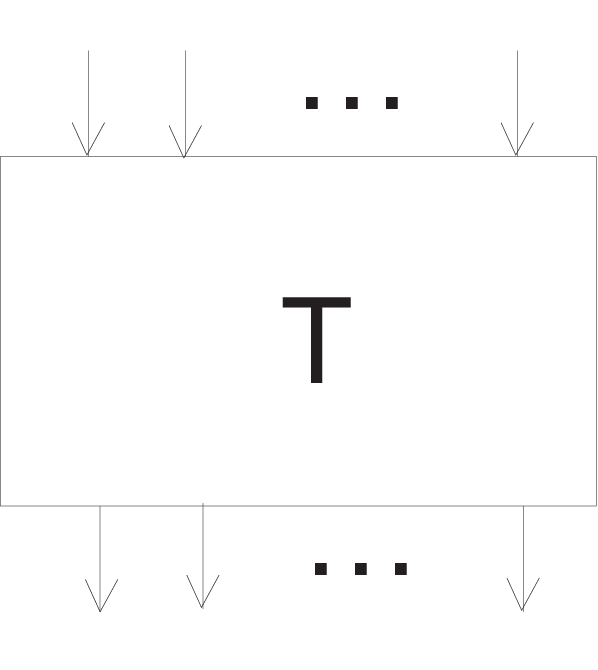
Set $T^{(n)}$ to be the element in $H_{n}(q,a)$ as illustrated in Figure 3, and let

(2.5)

\displaystyle t_{\lambda}=za\sum_{x\in\lambda}q^{2cn(x)}+\frac{a-a^{-1}}{z}.

where $cn(x)=j-i$ is the content of the cell in row $i$ and column $j$ of the Young diagram for the partition $\lambda$ . Then we have

(2.6)

\displaystyle T^{(n)}y_{\lambda}=t_{\lambda}y_{\lambda}.

Since a partition is uniquely determined by its contents, it is readily verified that $t_{\lambda}=t_{\mu}$ if and only if $\lambda=\mu$ .

Similarly, we set $T^{(n,m)}$ to be the analogue elements in $H_{n,m}(q,a)$ , and let

(2.7)

\displaystyle t_{\lambda,\mu}=z\left(a\sum_{x\in\lambda}q^{2cn(x)}-a^{-1}\sum_{x\in\mu}q^{-2cn(x)}\right)+\frac{a-a^{-1}}{z}.

It is also clear that $t_{\lambda,\mu}=t_{\lambda^{\prime},\mu^{\prime}}$ if and only if $\lambda=\lambda^{\prime}$ and $\mu=\mu^{\prime}$ .

2.1.3. The annulus

When $F$ is the annulus $S^{1}\times[0,1]$ , usually, we use $\mathcal{C}$ to denote the skein algebra $Sk(S^{1}\times[0,1])$ . $\mathcal{C}$ is a commutative algebra with the product induced by placing one annulus outside another.

The closure map $\hat{}:H_{n,m}(q,a)\rightarrow\mathcal{C}$ is an $R$ -linear map induced by taking an $(n,m)$ -tangle $T$ to its closure $\hat{T}$ in the annulus, whose image we call $\mathcal{C}^{(n,m)}$ . It is obvious that every diagram in the annulus represents an element in some $\mathcal{C}^{(n,m)}$ .

Turaev [91] showed that $\mathcal{C}$ is freely generated as an algebra by the set $\{A_{m}:m\in\mathbb{Z}\}$ where $A_{m},m\neq 0$ , is represented by the closure of the braid $\sigma_{|m|-1}\cdots\sigma_{2}\sigma_{1}$ . The orientation of the curve around the annulus is counter-clockwise for positive $m$ and clockwise for negative $m$ . The element $A_{0}$ is the identity element and is represented by the empty diagram. The algebra $\mathcal{C}$ is the product of two subalgebras $\mathcal{C}^{+}$ and $\mathcal{C}^{-}$ generated by $\{A_{m}:m\in\mathbb{Z},m\geq 0\}$ and $\{A_{m}:m\in\mathbb{Z},m\leq 0\}$ respectively.

Take a diagram $X$ in the annulus and link it once with a simple meridian loop, oriented in either direction, to give diagrams $\varphi(X)$ and $\bar{\varphi}(X)$ in the annulus. This induces linear endomorphisms $\varphi,\bar{\varphi}$ of the skein $\mathcal{C}$ , called the meridian maps. Each space $\mathcal{C}^{(n,m)}$ is invariant under $\varphi$ and $\bar{\varphi}$ . We set $\varphi^{(n)}=\varphi|_{\mathcal{C}^{(n)}}$ and $\varphi^{(n,m)}=\varphi|_{\mathcal{C}^{(n,m)}}$ .

Remark 2.6.

Rotating diagrams in the annulus $S^{1}\times I$ about the horizontal axis through the distinguished boundary points induces a linear automorphism of the skein $\mathcal{C}$ , which we denote by $*:\mathcal{C}\rightarrow\mathcal{C}$ . It is clear to see that $A_{m}^{*}=A_{-m}$ and then $(\mathcal{C}^{+})^{*}=\mathcal{C}^{-}$ and $(\mathcal{C}^{n,m})^{*}=\mathcal{C}^{m,n}$ .

The subspace $\mathcal{C}^{(n)}\subset\mathcal{C}^{+}$

The subspace $\mathcal{C}^{(n)}$ is spanned by monomials in $\{A_{m}\}$ , with $m\in\mathbb{Z}^{+}$ , of total weight $n$ , where the weight of $A_{m}$ is $m$ . It is clear that this spanning set consists of $\pi(n)$ elements, the number of partitions of $n$ . $\mathcal{C}^{+}$ is then graded as an algebra

(2.8)

\displaystyle\mathcal{C}^{+}=\bigoplus_{n=0}^{\infty}\mathcal{C}^{(n)}.

This subspace $\mathcal{C}^{+}$ can also viewed as the image of $H_{n}(q,a)$ under the closure map $\hat{}$ . Given the element $T^{(n)}\in H_{n}(q,a)$ as illustrated in Figure 3, take an element $S\in H_{n}(q,n)$ with $\hat{S}\in\mathcal{C}^{(n)}$ and compose it by $T^{(n)}$ . Then

(2.9)

\displaystyle\widehat{T^{(n)}S}=\varphi^{(n)}(\hat{S}).

Similarly,

(2.10)

\displaystyle\widehat{\bar{T}^{(n)}S}=\bar{\varphi}^{(n)}(\hat{S}).

Then it is easy to show that the eigenvalues of $\varphi^{(n)}$ are all distinct. Indeed, set $Q_{\lambda}=\widehat{y_{\lambda}}\in\mathcal{C}^{(n)}$ . Taking closures on both sides of the formula (2.6), we immediately obtain

(2.11)

\displaystyle\varphi^{(n)}(Q_{\lambda})=t_{\lambda}Q_{\lambda}.

The element $Q_{\lambda}$ is then an eigenvector of $\varphi^{(n)}$ with eigenvalue $t_{\lambda}$ . There are $\pi(n)$ of these eigenvectors, and the eigenvalues are all distinct. Hence all these $Q_{\lambda}$ are linear independent. Since $\mathcal{C}^{(n)}$ is spanned by $\pi(n)$ elements we can deduce that all the elements $Q_{\lambda}$ with $|\lambda|=n$ form a basis for $\mathcal{C}^{(n)}$ and that the eigenspaces are all $1$ -dimensional.

It was shown in [47, 48] that $Q_{\lambda}$ can be expressed as an explicit integral polynomial in $\{h_{m}\}_{m\geq 0}$ and $\mathcal{C}^{+}$ can be regarded as the ring of symmetric functions in variables $x_{1},..,x_{N},..$ with the coefficient ring $R$ . In this situation, $\mathcal{C}^{(n)}$ consists of the homogeneous functions of degree $n$ . The power sum $P_{n}=\sum x_{i}^{m}$ is a symmetric function which can be presented in terms of the complete symmetric functions, hence it represents a skein element which is also denoted by $P_{n}\in\mathcal{C}^{(m)}$ . Moreover, we have the identity

(2.12)

\displaystyle[m]P_{m}=X_{m}=\sum_{j=0}^{m-1}A_{m-1-j,j}

where $[m]=\frac{q^{m}-q^{-m}}{q-q^{-1}}$ and $A_{i,j}$ is the closure of the braid

\sigma_{i+j}\sigma_{i+j-1}\cdots\sigma_{j+1}\sigma_{j}^{-1}\cdots\sigma_{1}^{-1}.

Given a partition $\mu$ , we define

(2.13)

\displaystyle P_{\mu}=\prod_{i=1}^{l(\mu)}P_{\mu_{i}}.

According to the Frobenius formula for Schur function, we have

(2.14)

\displaystyle Q_{\lambda}=\sum_{\mu}\frac{\chi_{\lambda}(\mu)}{\mathfrak{z}_{\mu}}P_{\mu}.

The subspace $\mathcal{C}^{(n,m)}$

The image of $H_{n,m}(q,a)$ under the closure map is denoted by $\mathcal{C}^{(n,m)}\subset\mathcal{C}$ . Unlike the case for $\mathcal{C}^{(n)}$ where $\mathcal{C}^{(n)}\cap\mathcal{C}^{(n-1)}=\emptyset$ , we have that:

(2.15a)		$\displaystyle\mathcal{C}^{(n,m)}\supset\mathcal{C}^{(n-1,m-1)}\supset\cdots\supset$	$\displaystyle\mathcal{C}^{(n-m,0)},$	$\min(n,m)=m$ ,
	$\displaystyle\mathcal{C}^{(n,m)}\supset\mathcal{C}^{(n-1,m-1)}\supset\cdots\supset$	$\displaystyle\mathcal{C}^{(0,m-n)},$	$\min(n,m)=n$ .

and

(2.16)

\displaystyle\mathcal{C}^{(n,0)}=\mathcal{C}^{(n)}_{(+)},\ \mathcal{C}^{(0,m)}=\mathcal{C}^{(m)}_{(-)}.

where the subscripts indicate the direction of the strings around the center of the annulus. We have that $\mathcal{C}^{(n_{1},p_{1})}\cap\mathcal{C}^{(n_{2},p_{2})}=\emptyset$ if $n_{1}-m_{1}\neq n_{2}-m_{2}$ . Indeed, $\mathcal{C}^{(n,m)}$ is spanned by suitably weighted monomials in

(2.17)

\displaystyle\{A_{n},...,A_{1},A_{0},A_{-1},...,A_{-m}\}.

We can then see that

(2.18)

\displaystyle\mathcal{C}^{(n,m)}=\left(\mathcal{C}_{+}^{(n)}\times\mathcal{C}_{-}^{(m)}+\mathcal{C}^{(n-1,m-1)}\right).

The spanning set of $\mathcal{C}^{(n,m)}$ consists of $\pi(n,m)$ elements, where

(2.19)

\displaystyle\pi(n,m):=\sum_{j=0}^{k}\pi(n-j)\pi(m-j).

with $k=\min(n,m)$ .

Similar to grading of $\mathcal{C}^{+}$ with the $\mathcal{C}^{(n)}$ , the full skein $\mathcal{C}$ can be written in terms of $\mathcal{C}^{(n,m)}$ as follow:

(2.20)

\displaystyle\mathcal{C}=\bigoplus_{k=-\infty}^{\infty}\left(\bigcup_{n,m\geq 0}\{\mathcal{C}^{(n,m)}:n-m=k\}\right).

Now, we consider the meridian map:

(2.21)

\displaystyle\varphi^{(n,m)}:\mathcal{C}^{(n,m)}\rightarrow\mathcal{C}^{(n,m)}

It is proved in [69] that

Proposition 2.7 (See Theorem 6 in [69]).

$t_{\lambda,\mu}$ given by formula (2.7) with $|\lambda|\leq n,|\mu|\leq m$ and $|\lambda|-|\mu|=m$ are eigenvalues of the meridian map $\varphi^{(n,m)}$ , moreover, they occur with multiplicity $1$ .

A straightforward consequence is

Corollary 2.8.

There is a basis of $\mathcal{C}^{(n,m)}$ given by

(2.22)

\displaystyle\{Q_{\lambda,\mu}:|\lambda|\leq n,|\mu|\leq m,|\lambda|-|\mu|=n-m\}

such that $\varphi(Q_{\lambda,\mu})=t_{\lambda,\mu}Q_{\lambda,\mu}$ .

Then in [31], R. Hadji and H. Morton extended the method of [47, 48] and obtained the explicit expression for these basis elements $\{Q_{\lambda,\mu}\}$ .

Explicit expression for the basis elements $Q_{\lambda,\mu}$

Let element $h_{m}\in\mathcal{C}^{(m)}$ be the closure of the elements $\frac{1}{\alpha_{m}}a_{m}\in H_{m}(q,a)$ , i.e. $h_{m}=\frac{1}{\alpha_{m}}\hat{a}_{m}$ , where $a_{m}$ is the quasi-idempotent whose definition is given by formula (3.3), and $\alpha_{m}$ is the scalar given by $\alpha_{m}=q^{m(m-1)/2}\prod_{i=1}^{m}\frac{q^{i}-q^{-i}}{q-q^{-1}}\in R$ .

There is a readily defined involution on the skein $\mathcal{C}$ denoted by $*$ . It is the rotation of diagrams in the annulus $S^{1}\times[0,1]$ by $\pi$ about the horizontal axis through the distinguished boundary points. We can see that $(A_{m})^{*}=A_{-m}$ , so that $(\mathcal{C}^{+})^{*}=\mathcal{C}^{-}$ . Furthermore, $(\mathcal{C}^{(n,m)})^{*}=\mathcal{C}^{(m,n)}$ .

The skein $\mathcal{C}^{+}$ (resp. $\mathcal{C}^{-}$ ) is spanned by the monomials in $\{h_{m}\}_{m\geq 0}$ (resp. $\{h_{k}^{*}\}_{k\geq 0}$ ), indeed, the explicit relations between $\{h_{m}\}$ and the Turaev’s basis $\{A_{m}\}$ are presented in [68] (cf. Theorem 3.6 in [68]) and [71] (cf. Theorem 8 in [71] ). Then the whole skein $\mathcal{C}$ is spanned by the monomials in $\{h_{m},h_{k}^{*}\}_{m,k\geq 0}$ .

Given two partitions $\lambda,\mu$ with $l$ and $r$ parts. We first construct a $(l+r)\times(l+r)$ -matrix $M_{\lambda,\mu}$ with entries in $\{h_{m},h_{k}^{*}\}_{m,k\in\mathbb{Z}}$ as follows, where we have let $h_{m}=0$ if $m<0$ and $h_{k}^{*}=0$ if $k<0$ .

(2.23)

\displaystyle M_{\lambda,\mu}=\begin{pmatrix}h_{\mu_{r}}^{*}&h_{\mu_{r}-1}^{*}&\cdots&h_{\mu_{r}-r-l+1}^{*}\\ h_{\mu_{r-1}+1}^{*}&h_{\mu_{r-1}}^{*}&\cdots&h_{\mu_{r-1}-r-l}^{*}\\ \cdot&\cdot&\cdots&\cdot\\ h_{\mu_{1}+(r-1)}^{*}&h_{\mu_{1}+(r-2)}^{*}&\cdots&h_{\mu_{1}-l}^{*}\\ h_{\lambda_{1}-r}&h_{\lambda_{1}-(r-1)}&\cdots&h_{\lambda_{1}+l-1}\\ \cdot&\cdot&\cdots&\cdot\\ h_{\lambda_{l}-l-r+1}&h_{\lambda_{l}-s-r+2}&\cdots&h_{\lambda_{l}}\end{pmatrix}

It is easy to see that the subscripts of the diagonal entries in the $h$ -rows are the parts $\lambda_{1},\lambda_{2},...,\lambda_{l}$ of $\lambda$ in order, while the subscripts of the diagonal entries in the $h^{*}$ -rows are the parts $\mu_{1},\mu_{2},..,\mu_{r}$ of $\mu$ in reverse order.

Then, $Q_{\lambda,\mu}$ is defined as the determinant of the matrix $M_{\lambda,\mu}$ , i.e.

(2.24)

\displaystyle Q_{\lambda,\mu}=\det M_{\lambda,\mu}.

Example 2.9.

For two partitions $\lambda=(4,2,2)$ and $\mu=(3,2)$ , we have

(2.25)

\displaystyle Q_{\lambda,\mu}=\det\begin{pmatrix}h_{2}^{*}&h_{1}^{*}&1&0&0\\ h_{4}^{*}&h_{3}^{*}&h_{2}^{*}&h_{1}^{*}&1\\ h_{2}&h_{3}&h_{4}&h_{5}&h_{6}\\ 0&1&h_{1}&h_{2}&h_{3}\\ 0&0&1&h_{1}&h_{2}\end{pmatrix}.

Furthermore, we have

(2.26)

\displaystyle Q_{\lambda,\mu}=\sum_{\sigma,\rho,\nu}(-1)^{|\sigma|}c_{\sigma,\rho}^{\lambda}c_{\sigma^{t},\nu}^{\mu}Q_{\rho,\emptyset}Q_{\emptyset,\nu},

where $c_{\sigma,\rho}^{\lambda}$ is the Littlewood-Richardson coefficient which is determined by the product formula for Schur functions:

(2.27)

\displaystyle s_{\sigma}(\mathbf{x})s_{\rho}(\mathbf{x})=\sum_{\lambda}c_{\sigma,\rho}^{\lambda}s_{\lambda}(\mathbf{x}).

Moreover, the basis elements $Q_{\lambda,\mu}$ of $\mathcal{C}$ have the property that the product of any two is a non-negative integral linear combination of basis elements.

2.2. Colored HOMFLY-PT invariants

Let $\mathcal{L}$ be a framed link with $L$ components with a fixed numbering. For diagrams $Q_{1},..,Q_{L}$ in the skein model of annulus with the positive oriented core $\mathcal{C}^{+}$ , we define the decoration of $\mathcal{L}$ with $Q_{1},..,Q_{L}$ as the link

(2.28)

\displaystyle\mathcal{L}\star\otimes_{i=1}^{L}Q_{i}

which derived from $\mathcal{L}$ by replacing every annulus $\mathcal{L}$ by the annulus with the diagram $Q_{i}$ such that the orientations of the cores match. Each $Q_{i}$ has a small backboard neighborhood in the annulus which makes the decorated link $\mathcal{L}\otimes_{i=1}^{L}Q_{i}$ into a framed link. (see Figure 4 for a framed trefoil $\mathcal{K}$ decorated by skein element $\mathcal{Q}$ ).

The framed colored HOMFLY-PT polynomial of $\mathcal{L}$ is defined to be the framed HOMFLY-PT polynomial of the decorated link $\mathcal{L}\star\otimes_{i=1}^{L}Q_{i}$ which is given by

(2.29)

\displaystyle\mathcal{H}(\mathcal{L}\star\otimes_{i=1}^{L}Q_{i};q,a)=\langle\mathcal{L}\star\otimes_{i=1}^{L}Q_{i}\rangle.

In particular, if we choose $L$ basis elements $Q_{\lambda^{\alpha},\mu^{\alpha}}$ with $\alpha=1,...,L$ in the full skein $\mathcal{C}$ ,

Definition 2.10.

The framed full colored HOMFLY-PT invariant of the framed link $\mathcal{L}$ denoted by $\mathcal{H}_{[\vec{\lambda},\vec{\mu}]}(\mathcal{L};q,a)$ , is defined as the framed HOMFLY-PT polynomial of the decorated link $\mathcal{L}\star\otimes_{\alpha=1}^{L}Q_{\lambda^{\alpha},\mu^{\alpha}}$ , i.e.

(2.30)

\displaystyle\mathcal{H}_{[\vec{\lambda},\vec{\mu}]}(\mathcal{L};q,a):=\mathcal{H}(\mathcal{L}\star\otimes_{\alpha=1}^{L}Q_{\lambda^{\alpha},\mu^{\alpha}};q,a).

In particular, when all $\mu^{\alpha}=\emptyset$ , i.e. $Q_{\lambda^{\alpha},\emptyset}=Q_{\lambda^{\alpha}}$ . In this case, the framing factor for $Q_{\lambda}$ is given by $q^{-\kappa_{\lambda}}a^{-|\lambda|}$ . So we can add a framing factor to eliminate the framing dependency. It makes the framed colored HOMFLY-PT invariant $\mathcal{H}_{\vec{\lambda}}(\mathcal{L};q,a)$ into a framing independent invariant.

Definition 2.11.

The (framing independent) colored HOMFLY-PT invariant for the link $\mathcal{L}$ is given by

(2.31)

\displaystyle W_{\vec{\lambda}}(\mathcal{L};q,a)=q^{-\sum_{\alpha=1}^{L}\kappa_{\lambda^{\alpha}}|w(\mathcal{K_{\alpha}})|}a^{-\sum_{\alpha=1}^{L}|\lambda^{\alpha}|w(\mathcal{K}_{\alpha})}\mathcal{H}_{\vec{\lambda}}(\mathcal{L};q,a)

where $\vec{\lambda}=(\lambda^{1},..,\lambda^{L})\in\mathcal{P}^{L}$ .

Example 2.12.

For the unknot $U$ ,

(2.32)

\displaystyle W_{\mu}(U;q,a)=\mathcal{H}_{\mu}(U;q,a)=\prod_{x\in\mu}\frac{aq^{cn(x)}-a^{-1}q^{-cn(x)}}{q^{h(x)}-q^{-h(x)}}.

By the formula (2.26), we have

(2.33)

\displaystyle\mathcal{H}_{[\lambda,\mu]}(U;q,a)=\langle Q_{\lambda,\mu}\rangle=\sum_{\sigma,\rho,\nu}(-1)^{|\sigma|}c_{\sigma,\rho}^{\lambda}c_{\sigma^{t},\nu}^{\mu}W_{\rho}(U;q,a)W_{\nu}(U;q,a).

Definition 2.13.

Given a knot framed $\mathcal{K}$ , the normalized framed full HOMFLY-PT invariants of $\mathcal{K}$ is defined as follow

(2.34)

\displaystyle\mathcal{P}_{[\lambda,\mu]}(\mathcal{K};q,a)=\frac{\mathcal{H}_{[\lambda,\mu]}(\mathcal{K};q,a)}{\mathcal{H}_{[\lambda,\mu]}(U;q,a)}.

In other words,

(2.35)

\displaystyle\mathcal{H}_{[\lambda,\mu]}(\mathcal{K};q,a)=\mathcal{P}_{[\lambda,\mu]}(\mathcal{K};q,a)\mathcal{H}_{[\lambda,\mu]}(U;q,a).

If we draw the framed knot $\mathcal{K}$ in the annulus as the closure of a $1$ -tangle, then decorating it by $Q\in\mathcal{C}$ gives a diagram of $\mathcal{K}\star Q$ in the annulus, see Figure 5 for the case when $\mathcal{K}$ is the trefoil knot.

This construction induces a linear map $T_{\mathcal{K}}:\mathcal{C}\rightarrow\mathcal{C}$ . Suppose $Q$ is the eigenvector of $T_{\mathcal{K}}$ with eigenvalue $t_{\mathcal{K}}(q,a)$ , then

(2.36)

\displaystyle\mathcal{K}\star Q=T_{\mathcal{K}}(Q)=t({\mathcal{K}};q,a)Q=t({\mathcal{K}};q,a)U\star Q.

In particular, when $Q=Q_{\lambda,\mu}$ , taking the HOMFLY-PT polynomial, we obtain

(2.37)

\displaystyle t(\mathcal{K};q,a)=\frac{\mathcal{H}_{[\lambda,\mu]}(\mathcal{K};q,a)}{\mathcal{H}_{[\lambda,\mu]}(U;q,a)}

Therefore, $\mathcal{P}_{[\lambda,\mu]}(\mathcal{K};q,a)$ is also referred as the framed HOMFLY-PT 1-tangle invariants in [70].

For a link $\mathcal{L}$ with $L$ components, and let $\vec{\nu}=(\nu^{1},...,\nu^{L}),\ \vec{\lambda}=(\lambda^{1},...,\lambda^{L}),\vec{\mu}=(\mu^{1},...,\mu^{L})\in\mathcal{P}^{L}$ , set $c_{\vec{\lambda},\vec{\mu}}^{\vec{\nu}}=\prod_{\alpha=1}^{L}c_{\lambda^{\alpha},\mu^{\alpha}}^{\nu^{\alpha}}$ , where $c_{\lambda^{\alpha},\mu^{\alpha}}^{\nu^{\alpha}}$ is the Littlewood-Richardson coefficient.

Definition 2.14.

We define the framed composite invariants for $\mathcal{L}$ as follow

(2.38)

\displaystyle\mathcal{C}_{\vec{\nu}}(\mathcal{L};q,a)=\sum_{\vec{\lambda},\vec{\mu}}c_{\vec{\lambda},\vec{\mu}}^{\vec{\nu}}\mathcal{H}_{[\vec{\lambda},\vec{\mu}]}(\mathcal{L};q,a).

3. Idempotents in Hecke algebras

In this section, we first briefly review the skein theory construction of the idempotent of the Hecke algebra $H_{n}(q,a)$ follow [63]. Then we establish an important formula which will be used in the next section.

3.1. Young diagrams

Let $\lambda=(\lambda_{1},...,\lambda_{l})$ be a partition of $n$ , then $\lambda$ can be represented by a Young diagram which is a collection of $n$ cells arranged in rows, with $\lambda_{1}$ cells in the first row, $\lambda_{2}$ cells in the second row up to $\lambda_{l(\lambda)}$ . Usually, we denote both the partition and its Young diagram by $\lambda$ . The conjugate of $\lambda^{\vee}$ of $\lambda$ is the Young diagram whose rows form the columns of $\lambda$ . For the cell, in the $i$ -th row and $j$ -th column of $\lambda$ we write $(i,j)\in\lambda$ , and refer to $(i,j)$ as the coordinates of the cell.

A standard tableau $T^{\prime}(\lambda)$ is an assignment of the numbers $1$ to $n$ to the cells of $\lambda$ such that the numbers increase from left to right along the rows and top to bottom down the columns. In particular, $T(\lambda)$ will denote the tableau where the cells of the Young diagram are numbered from $1$ to $n$ along rows. Note that the transposition of rows and columns doesn’t take $T(\lambda)$ to $T(\lambda^{\vee})$ . We define the permutation $\pi_{\lambda}$ by $\pi_{\lambda}(i)=j$ where the transposition of $\lambda$ carries the cell $i$ in $T(\lambda)$ to the cell $j$ in $T(\lambda^{\vee})$ .

Let $\lambda$ and $\mu$ be Young diagrams with $|\lambda|=|\mu|=n$ . We say that a permutation $\pi\in S_{n}$ separates $\lambda$ from $\mu$ if no pair of numbers in the same row of $T(\lambda)$ are mapped by $\pi$ to the same row of $T(\mu)$ . For example, the permutation $\pi_{\lambda}$ separates $\lambda$ from its conjugate $\lambda^{\vee}$ .

Denoted by $R(\lambda)\subset S_{n}$ the subgroup of the permutations which preserve the rows of $T(\lambda)$ . It is easy to see that if $\pi$ separates $\lambda$ from $\mu$ then so does $\rho\pi\sigma$ for any $\rho\in R(\lambda)$ and $\sigma\in R(\mu)$ , and conversely, if $\pi$ separates $\lambda$ from $\lambda^{\vee}$ then $\pi=\rho\pi_{\lambda}\sigma$ with $\rho\in R(\lambda)$ and $\sigma\in R(\lambda^{\vee})$ . We say that $\lambda$ and $\mu$ are inseparable if no permutation $\pi\in S_{n}$ separates $\lambda$ from $\mu$ .

For every permutation $\pi\in S_{n}$ , there exists a unique braid $\omega_{\pi}$ ( called a positive permutation braid ) which is uniquely determined by the following properties:

(i) all strings are oriented from top to bottom;

(ii) for $i=1,...,n$ the $i$ -th string joins the point numbered $i$ at the top of the braid to the point numbered $\pi(i)$ at the bottom of the braid,

(iii) all the crossings occur with positive sign and each pair of strings cross at most once.

Lemma 3.1 (cf. [63]).

Let $\pi\in S_{n}$ be a permutation which separates $\lambda$ from $\lambda^{\vee}$ . Then there are $\rho\in R(\lambda)$ and $\sigma\in R(\lambda^{\vee})$ , such that

(3.1)

\displaystyle\omega_{\pi}=\omega_{\rho}\omega_{\pi_{\lambda}}\omega_{\sigma}.

Proof.

Since $\pi$ separates $\lambda$ from $\lambda^{\vee}$ , there are $\rho\in R(\lambda)$ and $\sigma\in R(\lambda^{\vee})$ , such that $\pi=\rho\pi_{\lambda}\sigma$ . By the definition of $\omega_{\pi_{\lambda}}$ , the pairs of strings which start in the same row of $T(\lambda)$ or end in the same row of $T(\lambda^{\vee})$ would never cross. The only pairs which cross in $\omega_{\rho}$ or $\omega_{\sigma}$ are in the same row of $T(\lambda)$ or $T(\lambda^{\vee})$ respectively. It follows that $\omega_{\rho}\omega_{\pi_{\lambda}}\omega_{\sigma}$ is a positive permutation braid. Hence $\omega_{\pi}=\omega_{\rho}\omega_{\pi_{\lambda}}\omega_{\sigma}.$ ∎

3.2. Constructions and properties

Let $F=R_{n}^{n}$ be a rectangle with $n$ inputs at the top and $n$ outputs at the bottom. Let $H_{n}(q,a)$ be the skein $Sk_{n}(R_{n}^{n})$ of $n$ -tangles. See Figure 6 for an element in $H_{n}(q,a)$ .

Composing $n$ -tangles by placing one above another induces a product which makes $H_{n}(q,a)$ into the Hecke algebra of type $A_{n-1}$ with the coefficients ring $R$ . $H_{n}(q,a)$ has a presentation generated by the elementary brads $\sigma_{1},...,\sigma_{n-1}$ subjects to relations

(3.2)		$\displaystyle\sigma_{i}\sigma_{j}=\sigma_{j}\sigma_{i},\ \ \ \ \|i-j\|\geq 2,$
	$\displaystyle\sigma_{i}\sigma_{i+1}\sigma_{i}=\sigma_{i+1}\sigma_{i}\sigma_{i+1}\ \ \ \|i-j\|=1$
	$\displaystyle(\sigma_{i}-q)(\sigma_{i}+q^{-1})=0,\ \ i=1,2,...,n-1.$

The Hecke algebra $H_{n}$ can be viewed as the quantum deformation of the group algebra $\mathbb{C}[S_{n}]$ of the symmetric group $S_{n}$ , whose idempotents are described by the classical Young symmetrisers. For a Young diagram $\lambda$ its Young symmetriser is the product of the sum of permutation which preserve the rows of $T(\lambda)$ and the alternating sum of permutations which preserve columns. In order to construct the idempotents in Hecke algebra, the idea is to make suitably quantum deformation of the classical Young symmetrisers. The two simplest idempotents in $H_{n}$ , corresponding to the single row and column Young diagrams, are given algebraically by Jones [36]. And the skein version of them are described by H. Morton [67] in terms of positive permutation braids $\omega_{\pi},\pi\in S_{n}$ . Then Gyoja [26] constructed the idempotents for general $\lambda$ . Finally, Morton and Aiston [63] provided skein theory construction of the idempotents in the HOMFLY-PT skein $H_{n}(q,a)$ .

We first define Jones’s row and column elements $a_{j}$ and $b_{j}$ , following the account in Morton [67]. Write $E_{n}(\sigma_{1},\sigma_{2},...,\sigma_{n-1})=\sum_{\pi\in S_{n}}\omega_{\pi}$ for the sum of positive permutation braids. We define

(3.3)		$\displaystyle a_{n}$	$\displaystyle=E_{n}(q\sigma_{1},q\sigma_{2},...,q\sigma_{n})=\sum_{\pi\in S_{n}}q^{l(\pi)}\omega_{\pi},$
	$\displaystyle b_{n}$	$\displaystyle=E_{n}(-q^{-1}\sigma_{1},-q^{-1}\sigma_{2},...,-q^{-1}\sigma_{n})=\sum_{\pi\in S_{n}}(-q)^{-l(\pi)}\omega_{\pi}.$

Lemma 3.2.

The element $a_{n}$ (resp. $b_{n}$ ) can be factorised in $H_{n}(q,a)$ with $\sigma_{i}+q^{-1}$ (resp. $\sigma_{i}-q$ ) as a left or a right factor for any $i\in\{1,2,..,n-1\}$ . If we define two linear homomorphisms $\varphi,\psi$ from the Hecke algebra $H_{n}(q,a)$ to the ring of scalars $R$ defined by $\varphi(\sigma_{i})=-q^{-1}$ and $\psi(\sigma_{i})=q$ for $i=1,...,n-1$ . Then for all $T\in H_{n}(q,a)$ , we have

(3.4)

\displaystyle a_{n}T=Ta_{n}=\psi(T)a_{n},\ b_{n}T=Tb_{n}=\varphi(T)b_{n}.

Proof.

This lemma was first proved in [67], for the sake of completeness, we provide the the proof here. Given $i\in\{1,2,,,.,n-1\}$ , we can pair the permutations as follows. For each permutation $\pi$ , consider its composite $\pi^{\prime}=\pi\circ(i,i+1)$ with transposition $(i,i+1)$ , then $\pi^{\prime}(i)=\pi(i+1)$ and $\pi^{\prime}(i+1)=\pi(i)$ . Hence exactly one of them preserves the order of $i$ and $i+1$ , and suppose it is $\pi$ such that $\pi(i)<\pi(i+1)$ . Consider the positive braids $\omega_{\pi}$ , and $\sigma_{i}=\omega_{(i,i+1)}$ , it is clear that $\omega_{\pi}\sigma_{i}$ is also a positive braid, then $\omega_{\pi^{\prime}}=\omega_{\pi}\sigma_{i}$ .

Therefore,

(3.5)	$\displaystyle a_{n}$	$\displaystyle=\sum_{\pi(i)<\pi(i+1)}q^{l(\pi)}\omega_{\pi}+\sum_{\pi^{\prime}(i)>\pi^{\prime}(i+1)}q^{l(\pi^{\prime})}\omega_{\pi^{\prime}}$
	$\displaystyle=\sum_{\pi(i)<\pi(i+1)}q^{l(\pi)}\omega_{\pi}+\sum_{\pi(i)<\pi(i+1)}q^{l(\pi)+1}\omega_{\pi}\sigma_{i}$
	$\displaystyle=a_{n}^{(i)}(1+q\sigma_{i}),$

where $a_{n}^{(i)}=\sum_{\pi(i)<\pi(i+1)}q^{l(\pi)}\omega_{\pi}$ .

By using the quadratic condition of Hecck algebra: $(\sigma_{i}+q^{-1})(\sigma_{i}-q)=0$ for $1\leq i\leq n-1$ , we have

(3.6)

\displaystyle a_{n}\sigma_{i}=a_{n}^{(i)}(1+q\sigma_{i})\sigma_{i}=qa_{n}^{i}(1+q\sigma_{i})=qa_{n}.

On the other hand side, for given $i\in\{1,...,n-1\}$ , one can also consider the composition of permutations $\pi^{\prime}=(i,i+1)\pi$ . Then

(3.7)	$\displaystyle a_{n}$	$\displaystyle=\sum_{\pi^{-1}(i)<\pi^{-1}(i+1)}q^{l(\pi)}\omega_{\pi}+\sum_{\pi^{\prime-1}(i)>\pi^{\prime-1}(i+1)}q^{l(\pi^{\prime})}\omega_{\pi^{\prime}}$
	$\displaystyle=\sum_{\pi^{-1}(i)<\pi^{-1}(i+1)}q^{l(\pi)}\omega_{\pi}+\sum_{\pi^{-1}(i)<\pi^{-1}(i+1)}q^{l(\pi)+1}\sigma_{i}\omega_{\pi}$
	$\displaystyle=(1+q\sigma_{i})\tilde{a}^{(i)}_{n},$

where $\tilde{a}^{(i)}_{n}=\sum_{\pi^{-1}(i)<\pi^{-1}(i+1)}q^{l(\pi)}\omega_{\pi}$ . By this formula we also obtain $\sigma_{i}a_{n}=qa_{n}$ . Hence we prove the formula (3.4), the proof of the second part of formula (3.4) is similar. ∎

Given a partition $\lambda=(\lambda_{1},...,\lambda_{l})$ of $n$ , we define

(3.8)		$\displaystyle E_{\lambda}$	$\displaystyle=a_{\lambda_{1}}\otimes a_{\lambda_{2}}\otimes\cdots\otimes a_{\lambda_{l}}$
(3.9)		$\displaystyle F_{\lambda}$	$\displaystyle=b_{\lambda_{1}}\otimes b_{\lambda_{2}}\otimes\cdots\otimes b_{\lambda_{l}}.$

Let $H_{\lambda}$ to the subalgebra of $H_{n}(q,a)$ generated by $\{\omega_{\rho},\rho\in R(\lambda)\}$ , then $E_{\lambda},F_{\lambda}\in H_{\lambda}$ and

(3.10)		$\displaystyle E_{\lambda}T$	$\displaystyle=TE_{\lambda}=\psi(T)E_{\lambda},$
	$\displaystyle F_{\lambda}T$	$\displaystyle=TF_{\lambda}=\varphi(T)F_{\lambda},$

for any $T\in H_{\lambda}$ by Lemma 3.2.

Lemma 3.3.

Let $\lambda$ and $\mu$ be two Young diagrams of $n$ cells, and let $\pi\in S_{n}$ be a permutation which does not separate $\lambda$ from $\mu$ . Then

(3.11)

\displaystyle E_{\lambda}\omega_{\pi}F_{\mu}=0=F_{\lambda}\omega_{\pi}E_{\mu}.

Proof.

This proof is essentially follows the Lemma 4.4 in [63]. Since $\pi$ does not separate $\lambda$ from $\mu$ , there are two cells in the same row of $\lambda$ which are sent to two cells in the same row of $\mu$ by $\pi$ . Then one can find $\rho\in R(\lambda)$ and $\sigma\in R(\mu)$ , such that $\pi^{\prime}=\rho\pi\sigma$ send the two adjacent cells $i$ and $i+1$ in the same row of $\lambda$ to the two adjacent cells $j$ and $j+1$ in the same row of $\mu$ . Then we have $\omega_{\pi}=T\omega_{\pi^{\prime}}T^{\prime}$ for some $T\in H_{\lambda}$ and $T^{\prime}\in H_{\mu}$ . Therefore,

(3.12)

\displaystyle E_{\lambda}\omega_{\pi}F_{\mu}=\psi(T)\varphi(T^{\prime})E_{\lambda}\omega_{\pi^{\prime}}F_{\mu}.

So we only need to show $E_{\lambda}\omega_{\pi^{\prime}}F_{\mu}=0$ . As to the permutation $\pi^{\prime}$ , we have $\pi^{\prime}(i+1)=\pi(i)+1=j+1$ , where $(ii+1)\in R(\lambda)$ and $(jj+1)\in R(\mu)$ . By the adjacency, we obtain $\sigma_{i}\omega_{\pi^{\prime}}=\omega_{\pi^{\prime}}\sigma_{j}.$ Hence,

(3.13)

\displaystyle(q^{-1}+\sigma_{i})\omega_{\pi^{\prime}}=\omega_{\pi^{\prime}}(q^{-1}+\sigma_{j}).

By formulas (3.5) and (3.7), we have $E_{\lambda}=T(q^{-1}+\sigma_{i})$ and $F_{\mu}=(q-\sigma_{j})T^{\prime}$ for some $T\in H_{\lambda}$ and $T^{\prime}\in H_{\mu}$ , then

(3.14)

\displaystyle E_{\lambda}\omega_{\pi^{\prime}}F_{\mu}=T(q^{-1}+\sigma_{i})\omega_{\pi^{\prime}}(q-\sigma_{j})T^{\prime}=T\omega_{\pi^{\prime}}(q^{-1}+\sigma_{j})(q-\sigma_{j})T^{\prime}=0.

The proof of the second identity in (3.11) is similar. ∎

Corollary 3.4.

Given a Young diagram $\lambda$ ,

	$\displaystyle E_{\lambda}\omega_{\pi}F_{\lambda^{\vee}}=$	$\displaystyle(-1)^{l(\sigma)}q^{l(\rho)-l(\sigma)}E_{\lambda}\omega_{\pi_{\lambda}}F_{\lambda^{\vee}},$	if $\omega_{\pi}=\omega_{\rho}\omega_{\pi_{\lambda}}\omega_{\sigma}$
	$\displaystyle E_{\lambda}\omega_{\pi}F_{\lambda^{\vee}}=$	$\displaystyle 0,$	otherwise .

and

	$\displaystyle F_{\lambda^{\vee}}\omega_{\pi}E_{\lambda}=$	$\displaystyle(-1)^{l(\sigma)}q^{l(\rho)-l(\sigma)}F_{\lambda^{\vee}}\omega_{\pi_{\lambda}^{-1}}E_{\lambda},$	if $\omega_{\pi}=\omega_{\sigma}\omega_{\pi_{\lambda}^{-1}}\omega_{\rho}$
	$\displaystyle F_{\lambda^{\vee}}\omega_{\pi}E_{\lambda}=$	$\displaystyle 0,$	otherwise .

for some $\rho\in R(\lambda),\sigma\in R(\lambda^{\vee})$

Proof.

By Lemma 3.3, if $\pi$ doesn’t separate $\lambda$ from $\lambda^{\vee}$ , then $E_{\lambda}\omega_{\pi}F_{\lambda^{\vee}}=0$ . Otherwise, there are some $\rho\in R(\lambda),\sigma\in R(\lambda^{\vee})$ , such that $\omega_{\pi}=\omega_{\rho}\omega_{\pi_{\lambda}}\omega_{\sigma}.$ Then

(3.17)

\displaystyle E_{\lambda}\omega_{\pi}F_{\lambda^{\vee}}=E_{\lambda}\omega_{\rho}\omega_{\pi_{\lambda}}\omega_{\sigma}F_{\lambda^{\vee}}=\psi(\omega_{\rho})\varphi(\omega_{\sigma})E_{\lambda}\omega_{\pi_{\lambda}}F_{\lambda^{\vee}}=(-1)^{l(\sigma)}q^{l(\rho)-l(\sigma)}E_{\lambda}\omega_{\pi_{\lambda}}F_{\lambda^{\vee}}.

Similarly, if $\pi$ doesn’t separate $\lambda^{\vee}$ from $\lambda$ , by Lemma 3.3, $F_{\lambda^{\vee}}\omega_{\pi}E_{\lambda}=0$ . Otherwise, there are some $\rho\in R(\lambda),\sigma\in R(\lambda^{\vee})$ such that $\omega_{\pi}=\omega_{\sigma}\omega_{\pi_{\lambda}^{-1}}\omega_{\rho}$ , since $\omega_{\pi_{\lambda^{\vee}}}=\omega_{\pi_{\lambda}^{-1}}$ separate $\lambda^{\vee}$ from $\lambda.$ Then we obtain the second formula. ∎

Lemma 3.5.

Given a Young diagram $\lambda$ ,

(3.18)

\displaystyle F_{\lambda^{\vee}}\omega_{\pi_{\lambda}^{-1}}E_{\lambda}=F_{\lambda^{\vee}}\overline{\omega}_{\pi_{\lambda}^{-1}}E_{\lambda}=F_{\lambda^{\vee}}\omega_{\pi_{\lambda}}^{-1}E_{\lambda}.

Proof.

Taking any one of crossings of $\omega_{\pi_{\lambda}^{-1}}$ , the skein relation gives

(3.19)

\displaystyle\omega_{\pi_{\lambda}^{-1}}=\omega^{\prime}_{\pi_{\lambda}^{-1}}-(q-q^{-1})L_{0},

where $L_{0}$ arises by smoothing this crossing. Clearly, the corresponding permutation determined by $L_{0}$ does not separate $\lambda^{\vee}$ from $\lambda$ . With a slight modification of the proof of Lemma 3.3, we have $F_{\lambda^{\vee}}L_{0}E_{\lambda}=0$ . Hence

(3.20)

\displaystyle F_{\lambda^{\vee}}\omega_{\pi_{\lambda}^{-1}}E_{\lambda}=F_{\lambda^{\vee}}\omega^{\prime}_{\pi_{\lambda}^{-1}}E_{\lambda}.

Then switch the other crossings in $\omega^{\prime}_{\pi_{\lambda}^{-1}}$ , using the above process inductively, we will obtain the formula (3.18).

∎

We now define the idempotent elements $y_{\lambda}\in H_{n}(q,a)$ for each partition $\lambda$ as follow. Let $e_{\lambda}=E_{\lambda}\omega_{\pi_{\lambda}}F_{\lambda^{\vee}}\omega_{\pi_{\lambda}}^{-1},$ then by using Lemma 3.3 and Corollary 3.4, it is straightforward to compute that $e_{\lambda}e_{\mu}=0$ for $\lambda\neq\mu$ , and

(3.21)

\displaystyle e_{\lambda}^{2}=\alpha_{\lambda}e_{\lambda}

for some scalar $\alpha_{\lambda}\in R$ . With the help of a formula established in [100] via $SU(N)$ skein theory, Aiston [1] computes that

(3.22)

\displaystyle\alpha_{\lambda}

\displaystyle=\prod_{(i,j)\in\lambda}q^{j-i}[\lambda_{i}+\lambda_{j}^{\vee}-i-j+1].

Then we define the idempotent $y_{\lambda}$ as follow

(3.23)

\displaystyle y_{\lambda}=\frac{1}{\alpha_{\lambda}}e_{\lambda}.

Finally, we prove the following proposition which will be used in the next section.

Proposition 3.6.

For any $\pi\in S_{n}$ , we have

	$\displaystyle y_{\lambda}\omega_{\pi}y_{\lambda}=$	$\displaystyle(-1)^{l(\sigma)}q^{l(\pi)-2l(\sigma)}y_{\lambda},$	if $\omega_{\pi}=\omega_{\pi_{\lambda}}\omega_{\sigma}\omega_{\pi_{\lambda}^{-1}}\omega_{\rho}$ for some $\rho\in R(\lambda),\sigma\in R(\lambda^{\vee})$
	$\displaystyle y_{\lambda}\omega_{\pi}y_{\lambda}=$	$\displaystyle 0,$	otherwise .

Proof.

We only need to compute $e_{\lambda}\omega_{\pi}e_{\lambda}$ . By the second formula in Corollary 3.4 and Lemma 3.5, when $\omega_{\pi}=\omega_{\pi_{\lambda}}\omega_{\sigma}\omega_{\pi_{\lambda}^{-1}}\omega_{\rho}$ , we obtain

(3.25)	$\displaystyle e_{\lambda}\omega_{\pi}e_{\lambda}$	$\displaystyle=E_{\lambda}\omega_{\pi_{\lambda}}F_{\lambda^{\vee}}\omega_{\pi_{\lambda}}^{-1}\omega_{\pi}E_{\lambda}\omega_{\pi_{\lambda}}F_{\lambda^{\vee}}\omega_{\pi_{\lambda}}^{-1}$
	$\displaystyle=E_{\lambda}\omega_{\pi_{\lambda}}F_{\lambda^{\vee}}\omega_{\sigma}\omega_{\pi_{\lambda}^{-1}}\omega_{\rho}E_{\lambda}\omega_{\pi_{\lambda}}F_{\lambda^{\vee}}\omega_{\pi_{\lambda}}^{-1}$
	$\displaystyle=(-1)^{l(\sigma)}q^{l(\rho)-l(\sigma)}E_{\lambda}\omega_{\pi_{\lambda}}F_{\lambda^{\vee}}\omega_{\pi_{\lambda}^{-1}}E_{\lambda}\omega_{\pi_{\lambda}}F_{\lambda^{\vee}}\omega_{\pi_{\lambda}}^{-1}$
	$\displaystyle=(-1)^{l(\sigma)}q^{l(\rho)-l(\sigma)}E_{\lambda}\omega_{\pi_{\lambda}}F_{\lambda^{\vee}}\omega_{\pi_{\lambda}}E_{\lambda}\omega_{\pi_{\lambda}}F_{\lambda^{\vee}}\omega_{\pi_{\lambda}}^{-1}$
	$\displaystyle=(-1)^{l(\sigma)}q^{l(\rho)-l(\sigma)}e_{\lambda}^{2}$
	$\displaystyle=(-1)^{l(\sigma)}q^{l(\rho)-l(\sigma)}\alpha_{\lambda}e_{\lambda}$
	$\displaystyle=(-1)^{l(\sigma)}q^{l(\pi)-2l(\sigma)}\alpha_{\lambda}e_{\lambda}.$

∎

4. Strong integrality theorem

4.1. Refined coefficient formula

In this subsection, we study the resolutions in the skein $H_{n,p}(q,a)$ carefully, and we obtain a refined formula for the coefficients appearing in the resolutions. We follow the notations in [70]. The diagram in a rectangle with $n$ outputs and $m$ inputs at the top, matched at the bottom are called $(n,m)$ -tangles. The resulting skein of the rectangle, denoted by $H_{n,m}(q,a)$ , is an algebra of dimension $(n+m)!$ over the ring $R$ , where the product is induced by placing one tangle above another.

A framed knot $\mathcal{K}$ can be represented as a 1-tangle $T(\mathcal{K})$ by a single knotted arc as in Figure 7 for $\mathcal{K}$ is the trefoil knot.

The $(n,m)$ -parallel of $T(\mathcal{K})$ , denoted by $T_{n,m}(\mathcal{K})$ in the skein $H_{n,m}(q,a)$ is constructed by drawing $n+m$ parallel oriented strands to the arc $T(\mathcal{K})$ , with $n$ oriented in one sense and $m$ in the other. Clearly, $T_{n,m}(\mathcal{K})\in H_{n,m}(q,a)$ .

Applying the standard resolution produces to the tangle $T_{n,m}(\mathcal{K})\in H_{n,m}(q,a)$ , we can write $T_{n,m}(\mathcal{K})$ as a $R$ -linear combination of $(n+m)!$ totally descending tangles without closed components. We denote the set of all such tangles by $S=\{T_{(i)}|i=1,...,(n+m)!\}$ . In particular, for case $m=0$ , such tangles are the positive permutation braids, denoted by $\{\omega_{\pi}:\pi\in S_{n}\}$ , with strings oriented from top to bottom, while for $n=0$ , they are the positive permutation braids, denoted by $\{\omega^{*}_{\rho}:\rho\in S_{m}\}$ , with string orientation from bottom to top.

For each tangle, we can count the number $k$ of its arcs which connects input and output points at the top. Then $0\leq k\leq\min(n,m)$ . We can divides the set $S$ into two parts

(4.1)

\displaystyle S=S^{(0)}\cup S^{(1)},

where $S^{(0)}$ consists tangles with $k=0$ in $S$ , while $S^{(1)}$ consists tangles with $k\geq 1$ in $S$ . In particular, the tangles with $k=0$ in $S^{(0)}$ have the form $\omega_{\pi}\otimes\omega_{\rho}^{*}$ for some $\pi\in S_{n}$ and $\rho\in S_{m}$ , where $\otimes$ denotes juxtaposition of tangles side by side.

We can write $T_{n,m}(\mathcal{K})$ in the skein $H_{n,m}(q,a)$ as

(4.2)

\displaystyle T_{n,m}(\mathcal{K})=T_{n,m}^{(0)}(\mathcal{K})+T_{n,m}^{(1)}(\mathcal{K})

where $T_{n,m}^{(0)}(\mathcal{K})$ is a combination of tangles in $S^{(0)}$ and $T_{n,m}^{(1)}(\mathcal{K})$ is a combination of tangles in $S^{(1)}$ . Then

(4.3)

\displaystyle T_{n,m}^{(0)}(\mathcal{K})=\sum_{\pi\in S_{n},\rho\in S_{m}}c_{\pi,\rho}(\mathcal{K})(\omega_{\pi}\otimes\omega_{\rho}^{*}),

and we have

Lemma 4.1.

$c_{\pi,\rho}(\mathcal{K})\in\mathbb{Z}[a^{\pm},z]$ and the powers of $z$ appearing in the coefficients $c_{\pi,\rho}(\mathcal{K})$ are simultaneously even (resp. odd) if $l(\pi)+l(\rho)$ is even (resp. odd).

Proof.

Given a $(n,m)$ -tangle $T$ , let $L(T)$ denote the number of the closed components of $T$ . Denote by $T^{\prime}$ the tangle after removing all the closed components of $T$ , let $l(T)$ be number of the components after closing the tangle $T^{\prime}$ . It is clear that $l(\omega_{\pi})=l(c(\pi))$ , the length of the partition $c(\pi)$ which denotes the cycle type of the permutation $\pi$ .

If we switch or smooth a crossing of sign $\pm 1$ in a tangle $T\in H_{n,m}(q,a)$ , we obtain tangles $T_{\mp}$ and $T_{0}$ which satisfy the skein relation

(4.4)

\displaystyle T=T_{\mp}\pm zT_{0}.

It is obvious that we have $l(T_{\mp})+L(T_{\mp})=l(T)+L(T)$ and $l(T_{0})+L(T_{0})=l(T)+L(T)\pm 1$ . Then

(4.5)

\displaystyle z^{l(T)+L(T)}T=z^{l(T_{\mp})+L(T_{\mp})}T_{\mp}\pm z^{\epsilon}z^{l(T_{0})+L(T_{0})}T_{0},

where $\epsilon$ takes the value $0$ or $2$ .

By induction and using Reidemeister moves, we obtain

(4.6)

\displaystyle z^{l(T)+L(T)}T=\sum_{\tilde{T}_{(i)}\in S}\tilde{c}_{(i)}z^{l(\tilde{T}_{(i)})+L(\tilde{T}_{(i)})}\tilde{T}_{(i)}

where $\tilde{c}_{(i)}\in\mathbb{Z}[a^{\pm 1},z^{2}]$ , $\tilde{T}_{(i)}$ is the tangle $T_{(i)}$ plus $L(\tilde{T}_{(i)})$ null-homotopic closed curves without crossings. Then $z^{L(\tilde{T}_{(i)})}\tilde{T}_{{}_{(i)}}=(a-a^{-1})^{L(\tilde{T}_{(i)})}T_{(i)}$ by removing these null-homotopic closed curves.

In conclusion, we have the following expansion for any $T\in H_{n,m}(q,a)$ ,

(4.7)

\displaystyle z^{l(T)+L(T)}T=\sum_{T_{(i)}\in S}c_{(i)}z^{l(T_{(i)})}T_{(i)},

with $c_{(i)}\in\mathbb{Z}[a^{\pm},z^{2}]$ .

In particular, for $T_{n,m}(\mathcal{K})\in H_{n,m}(q,a)$ , it easy to see that $L(T_{n,m}(\mathcal{K}))=0$ and $l(T_{n,m}(\mathcal{K}))=n+m$ , we have

(4.8)

\displaystyle T_{n,m}(\mathcal{K})

\displaystyle=\sum_{T_{(i)}\in S}c_{(i)}z^{l(T_{(i)})-(n+m)}T_{(i)}.

Since $S=S^{(0)}\cup S^{(1)}$ and $S^{(0)}=\{\omega_{\pi}\otimes\omega^{*}_{\rho}:\pi\in S_{n},\rho\in S_{m}\}$ , we obtain

(4.9)		$\displaystyle T_{n,m}(\mathcal{K})$	$\displaystyle=\sum_{\pi\in S_{n},\rho\in S_{p}}c_{\pi,\rho}z^{l(\omega_{\pi}\otimes\omega_{\rho}^{})-(n+m)}\omega_{\pi}\otimes\omega_{\rho}^{}$
		$\displaystyle+\sum_{T_{(i)}\in S^{(1)}}c_{(i)}z^{l(T_{(i)})-(n+m)}T_{(i)},$

with the coefficients $c_{\pi,\rho},c_{(i)}\in\mathbb{Z}[a^{\pm 1},z^{2}]$ .

Therefore, the coefficients $c_{\pi,\rho}(\mathcal{K})$ in formula (4.3) is given by

(4.10)

\displaystyle c_{\pi,\rho}(\mathcal{K})=c_{\pi,\rho}z^{l(\omega_{\pi}\otimes\omega_{\rho}^{*})-(n+m)}

Clearly, $l(\omega_{\pi}\otimes\omega_{\rho}^{*})=l(\omega_{\pi})+l(\omega_{\rho}^{*})=l(c(\pi))+l(c(\rho))$ . By the relation (4.12) which will be proved in the following Lemma 4.2, we obtain

(4.11)

\displaystyle c_{\pi,\rho}(\mathcal{K})=c_{\pi,\rho}z^{l(c(\pi))+l(c(\rho))-(n+p)}=c_{\pi,\rho}z^{l(\pi)+l(\rho)+2k}

for some $k\in\mathbb{Z}$ . Combining $c_{\pi,\rho}\in\mathbb{Z}[a^{\pm 1},z^{2}]$ , we complete the proof.

∎

Lemma 4.2.

Given a permutation $\pi\in S_{n}$ , we have the following identity

(4.12)

\displaystyle l(\pi)+l(c(\pi))=n\mod 2

Proof.

For every permutation $\pi\in S_{n}$ , its length $l(\pi)$ can be obtained by calculating the minimal number of the crossings in the positive braid $\omega_{\pi}$ . When $n=2$ , we have $S_{2}=\{\pi_{1}=(1)(2),\pi_{2}=(12)\}$ . Hence $c(\pi_{1})=(11)$ , and $c(\pi_{2})=(2)$ . It is clear that

(4.13)

\displaystyle l(\pi_{1})+l(c(\pi_{1}))=l(\pi_{2})+l(c(\pi_{2}))=2.

So Lemma 4.2 holds when $n=2$ .

Now we assume Lemma 4.2 holds for $n\leq d-1$ . As to $n=d$ , we consider a permutation $\pi\in S_{d}$ . We first study the special case, when $\pi$ has the cycle form: $\pi=\pi^{\prime}(d)$ , where $\pi^{\prime}$ is a permutation in $S_{d-1}$ . It is easy to see that $l(\pi)=l(\pi^{\prime})$ and $l(c(\pi))=l(c(\pi^{\prime}))+1$ . By the induction hypothesis, we have

(4.14)

\displaystyle l(\pi^{\prime})+l(c(\pi^{\prime}))=d-1\mod 2

Thus we get

(4.15)

\displaystyle l(\pi)+l(c(\pi))=d\mod 2.

Thus Lemma 4.2 holds for $\pi\in S_{d}$ with the cycle form $\pi^{\prime}(d)$ , $\pi^{\prime}\in S_{d-1}$ .

For the general case, we can assume $\pi$ has the cycle form $\pi=\sigma\tau$ , where $\tau$ is the cycle containing the element $d$ as the form $(i_{1}\cdots i_{j}d)$ for $\{i_{1},..i_{j}\}\subset\{1,..,d-1\}$ , $1\leq j\leq d-1$ , and $\sigma$ is a cycle in $S_{d-j-1}$ . Hence

(4.16)

\displaystyle l(c(\pi))=l(c(\sigma))+l(c(\tau)).

By the property of permutation, the number of the crossings between $\omega_{\sigma}$ and $\omega_{\tau}$ must be an even number, thus

(4.17)

\displaystyle l(\pi)=l(\sigma)+l(\tau)\mod 2.

Combining (4.16), (4.17) and the induction hypothesis, we have

(4.18)

\displaystyle l(\pi)+l(c(\pi))=d\mod 2.

So, we finish the proof of Lemma 4.2. ∎

Lemma 4.3.

The powers of $a$ in the coefficients $c_{\pi,\rho}(\mathcal{K})$ are simultaneously even (resp. odd) if $(n+m)w(\mathcal{K})$ is even (resp. odd).

Proof.

Applying the Reidemeister moves RII and RII moves and the HOMFLY-PT skein relation to diagram $T_{n,m}(\mathcal{K})$ in $H_{n,m}(q,a)$ , we will eventually obtain the final diagrams in the following forms: $T_{(i)}^{\alpha}\otimes U^{\otimes\beta}\otimes P^{\otimes\gamma}$ for $\alpha,\beta,\gamma\in\mathbb{N}$ , where $T_{(i)}^{\alpha}$ denotes the tangle $T_{(i)}$ with $\alpha$ positive kinks, $U$ denotes the unknot (i.e. trivial knot), $P$ denotes the unknot with one positive kink.

We let $S(\mathcal{K})$ be the set of all such final diagrams. Then, we have

(4.19)

\displaystyle T_{n,m}(\mathcal{K})=\sum_{T_{(i)}^{\alpha}\otimes U^{\otimes\beta}\otimes P^{\otimes\gamma}\in S(\mathcal{K})}c_{(i),\alpha,\beta,\gamma}(\mathcal{K})T_{(i)}^{\alpha}\otimes U^{\otimes\beta}\otimes P^{\otimes\gamma},

and the coefficients $c_{(i),\alpha,\beta,\gamma}(\mathcal{K})\in\mathbb{Z}[z]$ .

For any tangle $T\in H_{n,m}(q,a)$ , if we switch or smooth a crossing of sign $\pm 1$ in $T$ , we obtain tangles $T_{\pm 1}$ and $T_{0}$ . The key observation is that, we have

(4.20)		$\displaystyle w(T_{+})+L(T_{+})+l(T_{+})$	$\displaystyle=w(T_{-})+L(T_{-})+l(T_{-})\mod 2$
		$\displaystyle=w(T_{0})+L(T_{0})+l(T_{0})\mod 2.$

Therefore,

(4.21)		$\displaystyle w(T_{(i)}^{\alpha}\otimes U^{\otimes\beta}\otimes P^{\otimes\gamma})+L(T_{(i)}^{\alpha}\otimes U^{\otimes\beta}\otimes P^{\otimes\gamma})+l(T_{(i)}^{\alpha}\otimes U^{\otimes\beta}\otimes P^{\otimes\gamma})$
	$\displaystyle=w(T_{n,m}(\mathcal{K}))+L(T_{n,m}(\mathcal{K}))+l(T_{n,m}(\mathcal{K}))\mod 2$
	$\displaystyle=(n+m)^{2}w(\mathcal{K})+0+(n+m)\mod 2.$

In particular, when $T_{(i)}\in S^{(0)}$ , we know that $T_{(i)}=\omega_{\pi}\otimes\omega^{*}_{\rho}$ for some $\pi\in S_{n}$ and $\rho\in S_{m}$ . It is easy to get that

(4.22)		$\displaystyle w((\omega_{\pi}\otimes\omega_{\rho}^{*})^{\alpha}\otimes U^{\otimes\beta}\otimes P^{\otimes\gamma})$	$\displaystyle=l(\pi)+l(\rho)+\alpha+\gamma,$
	$\displaystyle L((\omega_{\pi}\otimes\omega_{\rho}^{*})^{\alpha}\otimes U^{\otimes\beta}\otimes P^{\otimes\gamma})$	$\displaystyle=\beta+\gamma,$
	$\displaystyle l((\omega_{\pi}\otimes\omega_{\rho}^{*})^{\alpha}\otimes U^{\otimes\beta}\otimes P^{\otimes\gamma})$	$\displaystyle=l(c(\pi))+l(c(\rho)).$

According to Lemma 4.2, we have

(4.23)		$\displaystyle l(\pi)+l(c(\pi))$	$\displaystyle=n\mod 2$
	$\displaystyle l(\rho)+l(c(\rho))$	$\displaystyle=p\mod 2$

Combining the formulas (4.21) and (4.22), we obtain

(4.24)

\displaystyle\alpha+\beta\equiv(n+m)^{2}w(\mathcal{K})\mod 2.

Finally, applying the Reidemeister move RI to the tangle $(\omega_{\pi}\otimes\omega_{\rho}^{*})^{\alpha}\otimes U^{\otimes\beta}\otimes P^{\otimes\gamma}$ , we obtain

(4.25)		$\displaystyle(\omega_{\pi}\otimes\omega_{\rho}^{*})^{\alpha}\otimes U^{\otimes\beta}\otimes P^{\otimes\gamma}$
	$\displaystyle=a^{\alpha+\gamma}(\omega_{\pi}\otimes\omega_{\rho}^{*})\otimes U^{\otimes\beta}\otimes U^{\otimes\gamma}$
	$\displaystyle=\frac{a^{\alpha+\gamma}(a-a^{-1})^{\beta+\gamma}}{z^{\beta+\gamma}}\omega_{\pi}\otimes\omega_{\rho}^{*}.$

It is obvious that the degrees of $a$ in the term $a^{\alpha+\gamma}(a-a^{-1})^{\beta+\gamma}$ have the same parity with $\alpha+\beta$ which is equal to $(n+m)^{2}w(\mathcal{K})$ mod 2. Note that the coefficient $c_{\pi,\rho}(\mathcal{K})$ is given by

(4.26)

\displaystyle c_{\pi,\rho}(\mathcal{K})=c_{(i),\alpha,\beta,\gamma}(\mathcal{K})\frac{a^{\alpha+\gamma}(a-a^{-1})^{\beta+\gamma}}{z^{\beta+\gamma}}

Therefore, the degrees of $a$ appearing in the coefficient $c_{\pi,\rho}(\mathcal{K})$ is equal to $(n+m)^{2}w(\mathcal{K})$ mod 2.

∎

In conclusion, combining Lemma 4.1 and Lemma 4.3 together, we obtain the following refined coefficient Theorem.

Theorem 4.4.

The coefficient $c_{\pi,\rho}(\mathcal{K})$ given by formula (4.3) satisfies the following strong integrality

(4.27)

\displaystyle c_{\pi,\rho}(\mathcal{K})\in q^{\epsilon_{1}}a^{\epsilon_{2}}\mathbb{Z}[q^{\pm 2},a^{\pm 2}],

where $\epsilon_{1},\epsilon_{2}\in\{0,1\}$ are determined by

(4.28)		$\displaystyle l(\pi)+l(\rho)$	$\displaystyle\equiv\epsilon_{1}\mod 2$
	$\displaystyle(n+m)w(\mathcal{K})$	$\displaystyle\equiv\epsilon_{2}\mod 2.$

4.2. Proof of the strong integrality theorem

In this subsection, we apply the technique used in [70] together with Proposition 3.6 and the refined coefficient Theorem 4.4 to prove the following strong integrality theorem.

Theorem 4.5.

For any framed knot $\mathcal{K}$ , the normalized framed full colored HOMFLY-PT invariant

(4.29)

\displaystyle\mathcal{P}_{[\lambda,\mu]}(\mathcal{K};q,a)\in a^{\epsilon}\mathbb{Z}[q^{\pm 2},a^{\pm 2}].

where $\epsilon\in\{0,1\}$ is determined by

(4.30)

\displaystyle(|\lambda|+|\mu|)w(\mathcal{K})

\displaystyle\equiv\epsilon\mod 2.

Proof.

First, it is easy to see that the meridian map $\varphi$ commutes with the map $T_{\mathcal{K}}$ . The eigenvalues of $\varphi$ are distinct and nonzero, then any eigenvector $Q_{\lambda,\mu}$ of $\varphi$ is also an eigenvector of $T_{\mathcal{K}}$ . Suppose $t(\lambda,\mu)$ is the eigenvalue of $T_{\mathcal{K}}$ for its eigenvector $Q_{\lambda,\mu}$ , By formula (2.36), we only need to prove the strong integrality for $t(\lambda,\mu)$ .

For $Q_{\lambda}\in\mathcal{C}_{|\lambda|,0}$ and $Q_{\mu}^{*}\in\mathcal{C}_{0,|\mu|}$ , their product $Q_{\lambda}Q_{\mu}^{*}\in\mathcal{C}_{|\lambda|,|\mu|}$ . It is shown in [31] that $Q_{\lambda,\mu}=Q_{\lambda}Q_{\mu}^{*}+W,$ where $W\in\mathcal{C}_{|\lambda|-1,|\mu|-1}$ . Since $T_{\mathcal{K}}(Q_{\lambda,\mu})=t(\lambda,\mu)Q_{\lambda,\mu},$ then

(4.31)

\displaystyle T_{\mathcal{K}}(Q_{\lambda}Q_{\mu}^{*})=t(\lambda,\mu)Q_{\lambda}Q_{\mu}^{*}+V

where $V\in\mathcal{C}_{|\lambda|-1,|\mu|-1}$ .

One can express $T_{\mathcal{K}}(Q_{\lambda}Q_{\mu}^{*})$ as the closure of the element $(y_{\lambda}\otimes y_{\mu}^{*})T_{n,m}(\mathcal{K})$ in $H_{n,m}(q,a)$ . By formula (4.2),

(4.32)

\displaystyle(y_{\lambda}\otimes y_{\mu}^{*})T_{n,m}(\mathcal{K})=(y_{\lambda}\otimes y_{\mu}^{*})T_{n,m}^{(0)}(\mathcal{K})+(y_{\lambda}\otimes y_{\mu}^{*})T_{n,m}^{(1)}(\mathcal{K}).

Clearly, the closure of $(y_{\lambda}\otimes y_{\mu}^{*})T_{n,m}^{(1)}(\mathcal{K})$ denoted by $V^{\prime}$ belongs to $\mathcal{C}_{n-1,m-1}$ , and

(4.33)

\displaystyle(y_{\lambda}\otimes y_{\mu}^{*})T_{n,m}^{(0)}(\mathcal{K})=\sum_{\pi\in S_{n},\rho\in S_{m}}c_{\pi,\rho}(\mathcal{K})(y_{\lambda}\omega_{\pi}\otimes y_{\mu}^{*}\omega_{\rho}^{*}).

Clearly, the closure of $y_{\lambda}\omega_{\pi}$ and $y_{\mu}^{*}\omega_{\rho}^{*}$ are equal to $c(\pi,\lambda)Q_{\lambda}$ and $c(\rho,\mu)Q_{\mu}^{*}$ . By Proposition 3.6, we have

(4.34)		$\displaystyle c(\pi,\lambda)$	$\displaystyle\in q^{l(\pi)}\mathbb{Z}[q^{2}],$
(4.35)		$\displaystyle c(\rho,\mu)$	$\displaystyle\in q^{l(\rho)}\mathbb{Z}[q^{2}].$

Therefore, the closure of $(y_{\lambda}\otimes y_{\mu}^{*})T_{n,m}^{(0)}(\mathcal{K})$ is equal to $C(\lambda,\mu)Q_{\lambda}Q_{\mu}^{*}$ , with

(4.36)

\displaystyle C(\lambda,\mu)=\sum_{\pi\in S_{n},\rho\in S_{m}}c_{\pi,\rho}(\mathcal{K})c(\pi,\lambda)c(\rho,\mu).

Hence we have

(4.37)

\displaystyle T_{\mathcal{K}}(Q_{\lambda}Q_{\mu}^{*})=C(\lambda,\mu)Q_{\lambda}Q_{\mu}^{*}+V^{\prime},

where $V^{\prime}\in\mathcal{C}_{n-1,m-1}$ .

Therefore, comparing with formula (4.31), $C(\lambda,\mu)=t(\lambda,\mu)$ is the normalized framed full colored HOMFLY-PT invariant. Applying Theorem 4.4 for the coefficients $c_{\pi,\rho}(\mathcal{K})$ and formulas (4.34) and (4.35), we obtain

(4.38)

\displaystyle C(\lambda,\mu)\in a^{\epsilon}\mathbb{Z}[q^{\pm 2},a^{\pm 2}].

where $\epsilon\in\{0,1\}$ is determined by

(4.39)

\displaystyle(|\lambda|+|\mu|)w(\mathcal{K})

\displaystyle\equiv\epsilon\mod 2.

∎

Remark 4.6.

In [45], T. Le proved the strong integrality for the normalized quantum group invariant of a knot $\mathcal{K}$ colored by an irreducible module over any simple Lie algebra $\mathfrak{g}$ via quantum group theory. It is easy to see Theorem 4.5 implies Le’s strong integrality when $\mathfrak{g}$ is the Lie algebra $sl_{N}\mathbb{C}$ .

Corollary 4.7.

For any framed knot $\mathcal{K}$ , we have

(4.40)		$\displaystyle\mathcal{H}_{[\lambda,\mu]}(\mathcal{K};-q,a)$	$\displaystyle=(-1)^{(\|\lambda\|+\|\mu\|)}\mathcal{H}_{[\lambda,\mu]}(\mathcal{K};q,a)$
(4.41)		$\displaystyle\mathcal{H}_{[\lambda,\mu]}(\mathcal{K};q,-a)$	$\displaystyle=(-1)^{(\|\lambda\|+\|\mu\|)(w(\mathcal{K})+1)}\mathcal{H}_{[\lambda,\mu]}(\mathcal{K};q,a).$

Proof.

Using the expression for the colored HOMFLY-PT invariant of unknot (2.32), it is straightforward to obtain

(4.42)		$\displaystyle W_{\lambda}(U;q,-a)$	$\displaystyle=(-1)^{\|\lambda\|}W_{\lambda}(U;q,a),$
(4.43)		$\displaystyle W_{\lambda}(U;-q,a)$	$\displaystyle=(-1)^{\|\lambda\|}W_{\lambda}(U;q,a),$

where in the second identity, we need to use the following identity for the partition $\lambda$ :

(4.44)

\displaystyle(-1)^{|\lambda|}=(-1)^{\sum_{x\in\lambda}(hl(x)+cn(x))}.

Then, by formula (2.33),

(4.45)		$\displaystyle\mathcal{H}_{[\lambda,\mu]}(U;q,-a)$	$\displaystyle=(-1)^{\|\lambda\|+\|\mu\|}\mathcal{H}_{[\lambda,\mu]}(U;q,a),$
(4.46)		$\displaystyle\mathcal{H}_{[\lambda,\mu]}(U;-q,a)$	$\displaystyle=(-1)^{\|\lambda\|+\|\mu\|}\mathcal{H}_{[\lambda,\mu]}(U;q,a).$

Finally, combining Theorem 4.5 and formula (2.35) together, we complete the proof. ∎

Corollary 4.8.

For any framed knot $\mathcal{K}$ , we have

(4.47)

\displaystyle\mathcal{H}_{[\lambda,\mu]}(\mathcal{K};q^{-1},a)=(-1)^{(|\lambda|+|\mu|)}\mathcal{H}_{[\lambda^{\vee},\mu^{\vee}]}(\mathcal{K};q,a)

Proof.

By using the formula (2.24) for $Q_{\lambda,\mu}$ ,

(4.48)

\displaystyle Q_{\lambda,\mu}|_{q\rightarrow-q^{-1}}=Q_{\lambda^{\vee},\mu^{\vee}},

It follows that

(4.49)

\displaystyle\mathcal{H}_{[\lambda,\mu]}(\mathcal{K};-q^{-1},a)=\mathcal{H}_{[\lambda^{\vee},\mu^{\vee}]}(\mathcal{K};q,a).

Then, combining with formula (4.40), we complete the proof. ∎

All the above formulas can be generalized to the case of link.

Theorem 4.9.

For any framed link $\mathcal{L}$ , we have

(4.50)	$\displaystyle\mathcal{H}_{[\vec{\lambda},\vec{\mu}]}(\mathcal{L};-q,a)$	$\displaystyle=(-1)^{\sum_{\alpha=1}^{L}(\|\lambda^{\alpha}\|+\|\mu^{\alpha}\|)}\mathcal{H}_{[\vec{\lambda},\vec{\mu}]}(\mathcal{L};q,a)$
(4.51)	$\displaystyle\mathcal{H}_{[\vec{\lambda},\vec{\mu}]}(\mathcal{L};q,-a)$	$\displaystyle=(-1)^{\sum_{\alpha=1}^{L}(\|\lambda^{\alpha}\|+\|\mu^{\alpha}\|)(w(\mathcal{K}_{\alpha})+1)}\mathcal{H}_{[\vec{\lambda},\vec{\mu}]}(\mathcal{L};q,a)$
(4.52)	$\displaystyle\mathcal{H}_{[\vec{\lambda},\vec{\mu}]}(\mathcal{L};q^{-1},a)$	$\displaystyle=(-1)^{\sum_{\alpha=1}^{L}(\|\lambda^{\alpha}\|+\|\mu^{\alpha}\|)}\mathcal{H}_{[\vec{\lambda}^{\vee},\vec{\mu}^{\vee}]}(\mathcal{L};q,a).$

Suppose $\mathcal{L}$ is a link with $L$ components $\mathcal{K}_{1},...,\mathcal{K}_{L}$ , we denote it by $\mathcal{L}=\mathcal{K}_{1}\bigvee\mathcal{K}_{2}\bigvee\cdots\bigvee\mathcal{K}_{L}$ . We cut the component $\mathcal{K}_{\alpha}$ open and get a 1-tangle, and we can draw $\mathcal{L}$ in the annulus as the closure of this 1-tangle. Decorating $\mathcal{K}_{\alpha}$ with a diagram $Q_{\alpha}$ gives a diagram $\mathcal{K}_{1}\bigvee\cdots\bigvee\mathcal{K}_{\alpha}\star Q_{\alpha}\bigvee\cdots\bigvee\mathcal{K}_{L}$ in $\mathcal{C}$ , it induces a linear map $T_{\mathcal{K}_{\alpha}}^{\mathcal{L}}:\mathcal{C}\rightarrow\mathcal{C}$ .

Similarly, the eigenvectors of $T_{\mathcal{K}_{\alpha}}^{\mathcal{L}}$ are given by $Q_{\lambda,\mu}$ , and we denote the eigenvalue of $T_{\mathcal{K}_{\alpha}}^{\mathcal{L}}$ corresponding to eigenvector $Q_{\lambda,\mu}$ by $t_{\mathcal{K}_{\alpha}}^{\mathcal{L}}(\lambda,\mu)$ .

Then the identity

(4.53)	$\displaystyle\mathcal{K}_{1}\bigvee\cdots\bigvee\mathcal{K}_{\alpha}\star Q_{\lambda,\mu}\bigvee\cdots\bigvee\mathcal{K}_{L}$	$\displaystyle=T_{\mathcal{K}_{\alpha}}^{\mathcal{L}}(Q_{\lambda,\mu})$
	$\displaystyle=t_{\mathcal{K}_{\alpha}}^{\mathcal{L}}(\lambda,\mu)Q_{\lambda,\mu}$
	$\displaystyle=t_{\mathcal{K}_{\alpha}}^{\mathcal{L}}(\lambda,\mu)U\star Q_{\lambda,\mu}$

implies that

(4.54)

\displaystyle t_{\mathcal{K}_{\alpha}}^{\mathcal{L}}(\lambda,\mu)=\frac{\mathcal{H}(\mathcal{K}_{1}\bigvee\cdots\bigvee\mathcal{K}_{\alpha}\star Q_{\lambda,\mu}\bigvee\cdots\bigvee\mathcal{K}_{L};q,a)}{\mathcal{H}(U\star Q_{\lambda,\mu};q,a)}.

With a slight modification of the proof of Theorem 4.5, one can show that

Proposition 4.10.

Under the above setting, we have

(4.55)

\displaystyle t_{\mathcal{K}_{\alpha}}^{\mathcal{L}}(\lambda,\mu)\in a^{\epsilon}\mathbb{Z}[q^{\pm 2},a^{\pm 2}].

where $\epsilon\in\{0,1\}$ is determined by

(4.56)

\displaystyle(|\lambda|+|\mu|)w(\mathcal{K}_{\alpha})+\sum_{\beta\neq\alpha}w(\mathcal{K}_{\beta})+(L-1)

\displaystyle\equiv\epsilon\mod 2.

By ormulas (2.26) and (2.14), we obtain

(4.57)		$\displaystyle Q_{\lambda,\mu}$	$\displaystyle=\sum_{\sigma,\rho,\nu}(-1)^{\|\sigma\|}c_{\sigma,\rho}^{\lambda}c_{\sigma^{t},\nu}^{\mu}Q_{\rho}Q_{\nu}^{*}$
		$\displaystyle=\sum_{\sigma,\rho,\nu,\tau,\delta}(-1)^{\|\sigma\|}c_{\sigma,\rho}^{\lambda}c_{\sigma^{t},\nu}^{\mu}\frac{\chi_{\rho}(\tau)}{\mathfrak{z}_{\tau}}\frac{\chi_{\nu}(\delta)}{\mathfrak{z}_{\delta}}\frac{1}{\{\tau\}\{\delta\}}X_{\tau}X_{\delta}^{*}.$

Therefore,

(4.58)	$\displaystyle\mathcal{\mathcal{L}}\star\otimes_{\beta=1}^{L}Q_{\lambda^{\alpha},\mu^{\alpha}}$	$\displaystyle=\mathcal{K}_{1}\star Q_{\lambda^{1},\mu^{1}}\bigvee\cdots\bigvee\mathcal{K}_{\alpha}\star Q_{\lambda^{\alpha},\mu^{\alpha}}\bigvee\cdots\bigvee\mathcal{K}_{L}\star Q_{\lambda^{L},\mu^{L}}$
	$\displaystyle=\sum_{\tau^{\beta},\delta^{\beta},\beta\neq\alpha}C_{\tau^{1},\delta^{1},..,\hat{\tau^{\alpha}},\hat{\delta^{\alpha}},..,\tau^{L},\delta^{L}}\prod_{\beta=1,\beta\neq\alpha}\frac{1}{\{\tau^{\beta}\}\{\delta^{\beta}\}}$
	$\displaystyle\cdot\mathcal{K}_{1}\star X_{\tau^{1}}X^{}_{\delta^{1}}\bigvee\cdots\bigvee\mathcal{K}_{\alpha}\star Q_{\lambda^{\alpha},\mu^{\alpha}}\bigvee\cdots\bigvee\mathcal{K}_{L}\star X_{\tau^{L}}X^{}_{\delta^{L}},$

where

(4.59)

\displaystyle C_{\tau^{1},\delta^{1},..,\hat{\tau^{\alpha}},\hat{\delta^{\alpha}},..,\tau^{L},\delta^{L}}=\sum_{\sigma^{\beta},\rho^{\beta},\nu^{\beta},\tau^{\beta},\delta^{\beta},\beta\neq\alpha}\prod_{\beta,\beta\neq\alpha}(-1)^{|\sigma^{\beta}|}c_{\sigma^{\beta},\rho^{\beta}}^{\lambda^{\beta}}c_{(\sigma^{\beta})^{t},\nu^{\beta}}^{\mu^{\beta}}\frac{\chi_{\rho^{\beta}}(\tau^{\beta})}{\mathfrak{z}_{\tau^{\beta}}}\frac{\chi_{\nu^{\beta}}(\delta^{\beta})}{\mathfrak{z}_{\delta^{\beta}}},

and $\hat{\tau^{\alpha}},\hat{\delta^{\alpha}}$ denote the indexes $\tau^{\alpha},\delta^{\alpha}$ do not appear in the summation.

We denote the link $\mathcal{L}_{\tau^{1},\delta^{1},..,\hat{\tau^{\alpha}},\hat{\delta^{\alpha}},..,\tau^{L},\delta^{L}}=\mathcal{K}_{1}\star X_{\tau^{1}}X^{*}_{\delta^{1}}\bigvee\cdots\bigvee\mathcal{K}_{\alpha}\bigvee\cdots\bigvee\mathcal{K}_{L}\star X_{\tau^{L}}X^{*}_{\delta^{L}}$ . By formula (4.55) and a careful computations of the writhe numbers for this link, we obtain

(4.60)

\displaystyle t_{\mathcal{K}_{\alpha}}^{\mathcal{L}_{\tau^{1},\delta^{1},..,\hat{\tau^{\alpha}},\hat{\delta^{\alpha}},..,\tau^{L},\delta^{L}}}(\lambda^{\alpha},\mu^{\alpha})\in a^{\epsilon}\mathbb{Z}[q^{\pm 2},a^{\pm 2}],

where $\epsilon\in\{0,1\}$ is determined by the following formula

(4.61)

\displaystyle(|\lambda^{\alpha}|+|\mu^{\alpha}|)w(\mathcal{K}_{\alpha})+\sum_{\beta\neq\alpha}(|\lambda^{\beta}|+|\mu^{\beta}|)(w(\mathcal{K}_{\beta})+1)\equiv\epsilon\mod 2.

Therefore,

(4.62)		$\displaystyle\mathcal{H}(\mathcal{\mathcal{L}}\star\otimes_{\beta=1}^{L}Q_{\lambda^{\alpha},\mu^{\alpha}};q,a)$	$\displaystyle=\sum_{\tau^{\beta},\delta^{\beta},\beta\neq\alpha}C_{\tau^{1},\delta^{1},..,\hat{\tau^{\alpha}},\hat{\delta^{\alpha}},..,\tau^{L},\delta^{L}}\prod_{\beta=1,\beta\neq\alpha}\frac{1}{\{\tau^{\beta}\}\{\delta^{\beta}\}}$
		$\displaystyle\cdot t_{\mathcal{K}_{\alpha}}^{\mathcal{L}_{\tau^{1},\delta^{1},..,\hat{\tau^{\alpha}},\hat{\delta^{\alpha}},..,\tau^{L},\delta^{L}}}(\lambda^{\alpha},\mu^{\alpha})\mathcal{H}(U\star Q_{\lambda^{\alpha},\mu^{\alpha}};q,a).$

Together with the formulas

(4.63)	$\displaystyle\mathcal{H}(U\star Q_{\lambda^{\alpha},\mu^{\alpha}};q,-a)$	$\displaystyle=(-1)^{\|\lambda^{\alpha}\|+\|\mu^{\alpha}\|}\mathcal{H}(U\star Q_{\lambda^{\alpha},\mu^{\alpha}};q,a),$
(4.64)	$\displaystyle\mathcal{H}(U\star Q_{\lambda^{\alpha},\mu^{\alpha}};-q,a)$	$\displaystyle=(-1)^{\|\lambda^{\alpha}\|+\|\mu^{\alpha}\|}\mathcal{H}(U\star Q_{\lambda^{\alpha},\mu^{\alpha}};q,a),$
(4.65)	$\displaystyle\mathcal{H}(U\star Q_{\lambda^{\alpha},\mu^{\alpha}};q,-a)$	$\displaystyle=(-1)^{\|\lambda^{\alpha}\|+\|\mu^{\alpha}\|}\mathcal{H}(U\star Q_{(\lambda^{\alpha})^{\vee},(\mu^{\alpha})^{\vee}};q,a).$

we finish the proof of Theorem 4.9.

5. Refined LMOV integrality structure

5.1. Symmetric functions and plethysms

Recall that the power sum symmetric function of infinite variables $\mathbf{x}=(x_{1},..,x_{N},..)$ is defined by $p_{n}(\mathbf{x})=\sum_{i}x_{i}^{n}.$ We refer to Section 8.1 for more detailed definitions about the symmetric functions. For a partition $\lambda=(\lambda_{1},...,\lambda_{l})$ , we define $p_{\lambda}(\mathbf{x})=\prod_{j=1}^{l}p_{\lambda_{j}}(\mathbf{x}).$ The Schur function $s_{\lambda}(\mathbf{x})$ is determined by the Frobenius formula

(5.1)

\displaystyle s_{\lambda}(\mathbf{x})=\sum_{\mu}\frac{\chi_{\lambda}(\mu)}{\mathfrak{z}_{\mu}}p_{\mu}(\mathbf{x}),

We let $\Lambda(\mathbf{x})$ be the ring of symmetric functions of $\mathbf{x}=(x_{1},x_{2},...)$ over the ring $\mathbb{Q}(q,a)$ , and let $\langle\cdot,\cdot\rangle$ be the Hall pair on $\Lambda(\mathbf{x})$ determined by

(5.2)

\displaystyle\langle s_{\lambda}(\mathbf{x}),s_{\mu}(\mathbf{x})\rangle=\delta_{\lambda,\mu}.

For $\vec{\mathbf{x}}=(\mathbf{x}^{1},...,\mathbf{x}^{L})$ , denote by $\Lambda(\vec{\mathbf{x}}):=\Lambda(\mathbf{x}^{1})\otimes_{\mathbb{Z}}\cdots\otimes_{\mathbb{Z}}\Lambda(\mathbf{x}^{L})$ the ring of functions separately symmetric in $\mathbf{x}^{1},...,\mathbf{x}^{L}$ , where $\mathbf{x}^{i}=(x^{i}_{1},x^{i}_{2},...)$ . We will study functions in the ring $\Lambda(\vec{\mathbf{x}})$ . For $\vec{\mu}=(\mu^{1},...,\mu^{L})\in\mathcal{P}^{L}$ , we let $a_{\vec{\mu}}(\vec{\mathbf{x}})=a_{\mu^{1}}(\mathbf{x}^{1})\cdots a_{\mu^{L}}(\mathbf{x}^{L})\in\Lambda(\vec{\mathbf{x}})$ be homogeneous of degree $(|\mu^{1}|,..,|\mu^{L}|)$ . Moreover, the Hall pair on $\Lambda(\vec{\mathbf{x}})$ is given by

(5.3)

\displaystyle\langle a_{1}(\mathbf{x}^{1})\cdots a_{L}(\mathbf{x}^{L}),b_{1}(\mathbf{x}^{1})\cdots b_{L}(\mathbf{x}^{L})\rangle=\langle a_{1}(\mathbf{x}^{1}),b_{1}(\mathbf{x}^{1})\rangle\cdots\langle a_{L}(\mathbf{x}^{n}),b_{L}(\mathbf{x}^{L})\rangle

for $a_{1}(\mathbf{x}^{1})\cdots a_{L}(\mathbf{x}^{L}),b_{1}(\mathbf{x}^{1})\cdots b_{L}(\mathbf{x}^{L})\in\Lambda(\vec{\mathbf{x}})$ . For $d\in\mathbb{Z}_{+}$ , we define the $d$ -th Adams operator $\Psi_{d}$ as the $\mathbb{Q}$ -algebra map on $\Lambda(\vec{\mathbf{x}})$

(5.4)

\displaystyle\Psi_{d}(f(\vec{\mathbf{x}};q,a))=f(\vec{\mathbf{x}}^{d};q^{d},a^{d}).

Denote by $\Lambda(\vec{\mathbf{x}})^{+}$ the set of symmetric functions with degree $\geq 1$ . The plethystic exponential Exp and logarithmic Log are inverse maps

(5.5)

\displaystyle\text{Exp}:\Lambda(\vec{\mathbf{x}})^{+}\rightarrow 1+\Lambda(\vec{\mathbf{x}})^{+},\ \text{Log}:1+\Lambda(\vec{\mathbf{x}})^{+}\rightarrow\Lambda(\vec{\mathbf{x}})^{+}

respectively defined by (see [32])

(5.6)

\displaystyle\text{Exp}(f)=\exp\left(\sum_{d\geq 1}\frac{\Psi_{d}(f)}{d}\right),\ \text{Log}(f)=\sum_{d\geq 1}\frac{\mu(d)}{d}\Psi_{d}(\log(f)),

where $\mu$ is the Möbius function. It is clear that

(5.7)

\displaystyle\text{Exp}(f+g)=\text{Exp}(f)\text{Exp}(g),\ \text{Log}(fg)=\text{Log}(f)+\text{Log}(g),

and Exp $(x)=\frac{1}{1-x}$ , if we use the expansion $\log(1-x)=-\sum_{d\geq 1}\frac{x^{d}}{d}$ .

5.2. LMOV functions

Consider a series of functions $S_{\vec{\lambda}}(q,a)\in\mathbb{Q}(q,a)$ , where $\vec{\lambda}\in\mathcal{P}^{L}$ , we introduce the partition function for $\{S_{\vec{\lambda}}(q,a)|\vec{\lambda}\in\mathcal{P}^{L}\}$ which is the following generating function

(5.8)

\displaystyle Z(\vec{\mathbf{x}};q,a)=\sum_{\vec{\lambda}\in\mathcal{P}^{L}}S_{\vec{\lambda}}(q,a)s_{\vec{\lambda}}(\vec{\mathbf{x}}).

Definition 5.1.

The LMOV function for the series $\{S_{\vec{\lambda}}(q,a)|\vec{\lambda}\in\mathcal{P}^{L}\}$ is given by

(5.9)

\displaystyle f_{\vec{\lambda}}(q,a)=\langle\text{Log}(Z(\vec{\mathbf{x}};q,a)),s_{\vec{\lambda}}(\vec{\mathbf{x}})\rangle

where $\langle\cdot,\cdot\rangle$ denotes the Hall pair in the ring of symmetric functions $\Lambda(\vec{\mathbf{x}})$ .

In particular, if we take $\mathbf{x}^{\alpha}=(x_{\alpha},0,0,...)$ for all $\alpha=1,...,L$ , i.e.

\vec{\mathbf{x}}=((x_{1},0,..),(x_{2},0,..),...,(x_{L},0,..)).

In this special case, we obtain the following special partition function for $\{S_{r_{1},...,r_{L}}(q,a)\}$ which is given by

(5.10)

\displaystyle\mathcal{Z}(x_{1},x_{2},...,x_{L};q,a)=\sum_{r_{1},...,r_{L}\geq 0}S_{r_{1},...,r_{L}}(q,a)x_{1}^{r_{1}}\cdots x_{L}^{r_{L}}.

Definition 5.2.

The special LMOV function for the series $\{S_{r_{1},...,r_{L}}(q,a)\}$ is

(5.11)

\displaystyle\mathfrak{f}_{n_{1},...,n_{L}}(q,a)=[x_{1}^{n_{1}}\cdots x_{L}^{n_{L}}]\text{Log}\mathcal{Z}(x_{1},x_{2},...,x_{L};q,a),

where the notation $[x_{1}^{n_{1}}\cdots x_{L}^{n_{L}}]f(x_{1},...,x_{L})$ denotes the coefficients of $x_{1}^{n_{1}}\cdots x_{L}^{n_{L}}$ in the function $f(x_{1},...,x_{L})$ .

We introduce the notion of $F$ -invariants $F_{\vec{\mu}}(q,a)$ (reps. $\mathcal{F}_{r_{1},...,r_{L}}(q,a)$ ) for $\{S_{\vec{\lambda}}(q,a)\}$ (resp. $\{S_{r_{1},...,r_{L}}(q,a)\}$ ) which is determined by the formula

(5.12)

\displaystyle\log Z(\vec{\mathbf{x}};q,a)=\sum_{\vec{\mu}}F_{\vec{\mu}}(q,a)p_{\vec{\mu}}(\vec{\bf{x}})

(resp. $\log\mathcal{Z}(x_{1},x_{2},...,x_{L};q,a)=\sum_{r_{1},...,r_{L}\geq 0}\mathcal{F}_{r_{1},...,r_{L}}(q,a)x_{1}^{r_{1}}\cdots x_{L}^{r_{L}}$ ).

Then, by the formula (8.10) in the Appendix Section 8, we obtain

(5.13)

\displaystyle F_{\vec{\mu}}(q,a)=\sum_{\Lambda\in\mathcal{P}(\mathcal{P}^{L}),|\Lambda|=\vec{\mu}\in\mathcal{P}^{L}}\Theta_{\Lambda}Z_{\Lambda}.

and

(5.14)

\displaystyle\mathcal{F}_{r_{1},...,r_{L}}(q,a)=\sum_{|\Lambda|=(r_{1},..,r_{L})}\Theta_{\Lambda}S_{\Lambda}(q,a).

By a straightforward computation, we obtain

(5.15)	$\displaystyle f_{\vec{\lambda}}(q,a)$	$\displaystyle=\langle Log(Z),s_{\vec{\lambda}}(\vec{\mathbf{x}})\rangle$
	$\displaystyle=\langle\sum_{d\geq 1}\frac{\mu(d)}{d}\circ\Psi_{d}(\sum_{\vec{\mu}}F_{\vec{\mu}}(q,a)p_{\vec{\mu}}(\mathbf{x})),s_{\vec{\lambda}}(\vec{\mathbf{x}})\rangle$
	$\displaystyle=\langle\sum_{d\geq 1}\frac{\mu(d)}{d}\sum_{\vec{\mu}}F_{\vec{\mu}}(q^{d},a^{d})p_{d\vec{\mu}}(\vec{\mathbf{x}}),s_{\vec{\lambda}}(\vec{\mathbf{x}})\rangle$
	$\displaystyle=\langle\sum_{d\geq 1}\frac{\mu(d)}{d}\sum_{\vec{\mu}}F_{\vec{\mu}}(q^{d},a^{d})\sum_{\vec{\nu}}\chi_{\vec{\nu}}(d\cdot\vec{\mu})s_{\vec{\nu}}(\vec{\mathbf{x}}),s_{\vec{\lambda}}(\vec{\mathbf{x}})\rangle$
	$\displaystyle=\sum_{\vec{\mu}}\chi_{\vec{\lambda}}(\vec{\mu})\sum_{d\|\vec{\mu}}\frac{\mu(d)}{d}F_{\vec{\mu}/d}(q^{d},a^{d}),$

and

(5.16)

\displaystyle\mathfrak{f}_{n_{1},...,n_{L}}(q,\vec{a})=\sum_{d\geq 1}\frac{\mu(d)}{d}\mathcal{F}_{\vec{n}/d}(q^{d},a^{d}).

Remark 5.3.

Here we mention that when $\vec{\lambda}=(\lambda^{1},...,\lambda^{L})=((n_{1}),...,(n_{L}))$ , according to their definitions, $f_{n_{1},...,n_{L}}(q,a)\neq\mathfrak{f}_{n_{1},...,n_{L}}(q,a).$ That’s why we use the different symbols there.

Definition 5.4.

We define the reformulated LMOV function for $\{S_{\vec{\lambda}}(q,a)\}$ as a character transformation of the LMOV functions,

(5.17)

\displaystyle g_{\vec{\mu}}(q,a)=\frac{1}{\{\vec{\mu}\}}\sum_{\vec{\lambda}}f_{\vec{\lambda}}(q,a)\chi_{\vec{\lambda}}(\vec{\mu}).

Plugging the formula (5.15) into 5.17, we obtain

(5.18)

\displaystyle g_{\vec{\mu}}(q,\vec{a})=\frac{\mathfrak{z}_{\vec{\mu}}}{\{\vec{\mu}\}}\sum_{d|\vec{\mu}}\frac{\mu(d)}{d}F_{\vec{\mu}/d}(q^{d},\vec{a}^{d}).

Remark 5.5.

The original definition of the reformulated LMOV function [55, 54, 56] is slightly different from here. They introduce the formula $T_{\lambda\mu}(\mathbf{x})=\sum_{\nu}\frac{\chi_{\lambda}(\nu)\chi_{\mu}(\nu)}{\mathfrak{z}_{\nu}}p_{\nu}(\mathbf{x}).$ In particularly, $T_{\lambda\mu}(q^{\rho})=\sum_{\mu}\frac{\chi_{\lambda}(\nu)\chi_{\mu}(\nu)}{\mathfrak{z}_{\nu}}\prod_{i=1}^{l(\nu)}\frac{1}{\{\nu_{i}\}},$ if one lets $q^{\rho}=(q^{-1},q^{-3},q^{-5},...)$ . In [55, 54, 56], the reformulated LMOV function for $\{S_{\vec{\lambda}}(q,a)\}$ is defined as $\hat{f}_{\vec{\mu}}(q,a)=\sum_{\vec{\lambda}}f_{\vec{\lambda}}(q,a)T_{\vec{\lambda}\vec{\mu}}(q^{\rho}).$ Therefore, we have

(5.19)

\displaystyle\hat{f}_{\vec{\lambda}}(q,a)=\chi_{\vec{\lambda}}(\vec{\mu})\sum_{\vec{\mu}}\frac{1}{\{\vec{\mu}\}}\sum_{d|\vec{\mu}}\frac{\mu(d)}{d}F_{\vec{\mu}/d}(q^{d},a^{d}).

It is obvious that two definitions by formulas (5.17) and (5.19) are related by a character transformation

(5.20)

\displaystyle g_{\vec{\mu}}(q,a)=\sum_{\vec{\lambda}}\chi_{\vec{\lambda}}(\vec{\mu})\hat{f}_{\vec{\lambda}}(q,a).

5.3. Refined LMOV conjecture

Given a framed link $\mathcal{L}$ with $L$ components $\mathcal{K}_{1},...,\mathcal{K}_{L}$ . Denote by $\vec{\tau}=(\tau^{1},...,\tau^{L})\in\mathbb{Z}^{L}$ the framing of $\mathcal{L}$ , i.e. $\tau^{\alpha}=w(\mathcal{K}_{\alpha})$ for $\alpha=1,...,L$ . In the following, we use the notation $\mathcal{L}_{\vec{\tau}}$ to denote this framed link $\mathcal{L}$ if we want to emphasize its framing.

For $\vec{\lambda}=(\lambda^{1},...,\lambda^{L}),\vec{\mu}=(\mu^{1},...,\mu^{L}),\vec{\nu}=(\nu^{1},...,\nu^{L})\in\mathcal{P}^{L}$ , set $c_{\vec{\lambda},\vec{\mu}}^{\vec{\nu}}=\prod_{\alpha=1}^{L}c_{\lambda^{\alpha},\mu^{\alpha}}^{\nu^{\alpha}}$ , where $c_{\lambda^{\alpha},\mu^{\alpha}}^{\nu^{\alpha}}$ is the Littlewood-Richardson coefficient.

Definition 5.6.

The $\tau$ -framed full colored HOMFLY-PT invariants for the framed link $\mathcal{L}_{\vec{\tau}}$ is given by

(5.21)

\displaystyle H_{\vec{\lambda}}(\mathcal{L}_{\vec{\tau}};q,a)=(-1)^{\sum_{\alpha=1}^{L}|\lambda^{\alpha}|\tau^{\alpha}}a^{-\sum_{\alpha=1}^{L}|\lambda^{\alpha}|\tau^{\alpha}}\mathcal{H}_{\vec{\lambda}}(\mathcal{L}_{\vec{\tau}};q,a).

Definition 5.7.

The $\tau$ -framed composite invariant for $\mathcal{L}_{\vec{\tau}}$ is given as follow

(5.22)

\displaystyle C_{\vec{\nu}}(\mathcal{L}_{\vec{\tau}};q,a)=(-1)^{\sum_{\alpha=1}^{L}|\lambda^{\alpha}|\tau^{\alpha}}\sum_{\vec{\lambda},\vec{\mu}}a^{-\sum_{\alpha=1}^{L}|\nu^{\alpha}|\tau^{\alpha}}c_{\vec{\lambda},\vec{\mu}}^{\vec{\nu}}\mathcal{H}_{[\vec{\lambda},\vec{\mu}]}(\mathcal{L}_{\vec{\tau}};q,a).

By using Theorem 4.9, we obtain

(5.23)		$\displaystyle H_{\vec{\lambda}}(\mathcal{L}_{\vec{\tau}};q,-a)$	$\displaystyle=(-1)^{\|\vec{\lambda}\|}H_{\vec{\lambda}}(\mathcal{L}_{\vec{\tau}};q,a),$
	$\displaystyle H_{\vec{\lambda}}(\mathcal{L}_{\vec{\tau}};-q,a)$	$\displaystyle=(-1)^{\|\vec{\lambda}\|}H_{\vec{\lambda}}(\mathcal{L}_{\vec{\tau}};q,a),$
	$\displaystyle H_{\vec{\lambda}}(\mathcal{L}_{\vec{\tau}};q^{-1},a)$	$\displaystyle=(-1)^{\|\vec{\lambda}\|}H_{\vec{\lambda^{t}}}(\mathcal{L}_{\vec{\tau}};q,a),$

and which hold similarly for the framed composite invariant $C_{\vec{\nu}}(\mathcal{L}_{\vec{\tau}};q,a)$ .

We denote the reformulated LMOV functions for $\tau$ -framed colored HOMFLY-PT invariants $\{H_{\vec{\lambda}}(\mathcal{L}_{\vec{\tau}};q,a)\}$ and $\tau$ -framed composite invariants $\{C_{\vec{\nu}}(\mathcal{L}_{\vec{\tau}};q,a)\}$ by $g_{\vec{\mu}}^{(0)}(\mathcal{L}_{\vec{\tau}};q,a)$ and $g_{\vec{\mu}}^{(1)}(\mathcal{L}_{\vec{\tau}};q,a)$ respectively.

Similarly, we write $\mathfrak{f}^{(0)}_{\vec{n}}(\mathcal{L}_{\vec{\tau}};q,a)$ and $\mathfrak{f}^{(1)}_{\vec{n}}(\mathcal{L}_{\vec{\tau}};q,a)$ for the corresponding special LMOV functions for the $\tau$ -framed colored HOMFLY-PT invariants $\{H_{\vec{r}}(\mathcal{L}_{\vec{\tau}};q,a)\}$ and composite invariants $\{C_{\vec{r}}(\mathcal{L}_{\vec{\tau}};q,a)\}$ respectively.

By formula (5.23), we obtain that the corresponding $F$ -invariants satisfies

(5.24)		$\displaystyle F_{\vec{\mu}}^{(h)}(\mathcal{L}_{\vec{\tau}};q,-a)$	$\displaystyle=(-1)^{\|\vec{\mu}\|}F_{\vec{\mu}}^{(h)}(\mathcal{L}_{\vec{\tau}};q,a),$
	$\displaystyle F_{\vec{\mu}}^{(h)}(\mathcal{L}_{\vec{\tau}};-q,a)$	$\displaystyle=(-1)^{\|\vec{\mu}\|}F_{\vec{\mu}}^{(h)}(\mathcal{L}_{\vec{\tau}};q,a),$
	$\displaystyle F_{\vec{\mu}}^{(h)}(\mathcal{L}_{\vec{\tau}};q^{-1},a)$	$\displaystyle=(-1)^{\|\vec{\mu}\|}F_{\vec{\mu}}^{(h)}(\mathcal{L}_{\vec{\tau}};q,a).$

and these symmetries similarly hold for $\mathcal{F}_{\vec{n}}^{(h)}(\mathcal{L}_{\vec{\tau}};q,-a).$

It follows that

(5.25)		$\displaystyle g^{(h)}_{\vec{\mu}}(\mathcal{L}_{\vec{\tau}};q,-a)$	$\displaystyle=(-1)^{\|\vec{\mu}\|}g^{(h)}_{\vec{\mu}}(\mathcal{L}_{\vec{\tau}};q,a),$
	$\displaystyle g^{(h)}_{\vec{\mu}}(\mathcal{L}_{\vec{\tau}};-q,a)$	$\displaystyle=g^{(h)}_{\vec{\mu}}(\mathcal{L}_{\vec{\tau}};q,a),$
	$\displaystyle g^{(h)}_{\vec{\mu}}(\mathcal{L}_{\vec{\tau}};q^{-1},a)$	$\displaystyle=g^{(h)}_{\vec{\mu}}(\mathcal{L}_{\vec{\tau}};q,a).$

and

(5.26)		$\displaystyle\mathfrak{f}^{(h)}_{\vec{n}}(\mathcal{L}_{\vec{\tau}};q,-a)$	$\displaystyle=(-1)^{\|\vec{n}\|}\mathfrak{f}^{(h)}_{\vec{n}}(\mathcal{L}_{\vec{\tau}};q,a),$
	$\displaystyle\mathfrak{f}^{(h)}_{\vec{n}}(\mathcal{L}_{\vec{\tau}};-q,a)$	$\displaystyle=(-1)^{\|\vec{n}\|}\mathfrak{f}^{(h)}_{\vec{n}}(\mathcal{L}_{\vec{\tau}};q,a),$
	$\displaystyle\mathfrak{f}^{(h)}_{\vec{n}}(\mathcal{L}_{\vec{\tau}};q^{-1},a)$	$\displaystyle=(-1)^{\|\vec{n}\|}\mathfrak{f}^{(h)}_{\vec{n}}(\mathcal{L}_{\vec{\tau}};q,a).$

for both $h=0$ and $1$ .

Remark 5.8.

We know that $g^{(h)}_{\vec{\mu}}(\mathcal{L}_{\vec{\tau}};q,a)$ belongs to the ring $\mathbb{Q}[q^{\pm},a^{\pm}]$ with the $(q^{r}-q^{-r})$ as its denominators, formula (5.25) implies that there exists some $d_{0}\in\mathbb{N}$ , such that

(5.27)

\displaystyle g^{(h)}_{\vec{\mu}}(\mathcal{L}_{\vec{\tau}};q,a)\in z^{-2d_{0}}a^{\epsilon}\mathbb{Q}[[z^{2}]][a^{\pm 2}]

where $\epsilon\in\{0,1\}$ which is determined by $|\vec{\mu}|\equiv\epsilon\mod 2$ .

From formula (4.62), we know that for $\vec{\lambda}\neq\vec{0}$ , both $H_{\vec{\lambda}}(\mathcal{L}_{\vec{\tau}};q,a)$ and $C_{\vec{\lambda}}(\mathcal{L}_{\vec{\tau}};q,a)$ contain a factor $\frac{a-a^{-1}}{q-q^{-1}}$ . We obtain

Theorem 5.9.

The reformulated LMOV functions $g^{(h)}_{\vec{\mu}}(\mathcal{L}_{\vec{\tau}};q,a)$ for both $h=0$ and $1$ can be written in the following form

(5.28)

\displaystyle g^{(h)}_{\vec{\mu}}(\mathcal{L}_{\vec{\tau}};q,a)=(a-a^{-1})\tilde{g}^{(h)}_{\vec{\mu}}(\mathcal{L}_{\vec{\tau}};q,a),

and $\tilde{g}^{(h)}_{\vec{\mu}}(\mathcal{L}_{\vec{\tau}};q,a)$ has the properties

(5.29)	$\displaystyle\tilde{g}^{(h)}_{\vec{\mu}}(\mathcal{L}_{\vec{\tau}};q,-a)$	$\displaystyle=(-1)^{\|\vec{\mu}\|-1}\tilde{g}^{(h)}_{\vec{\mu}}(\mathcal{L}_{\vec{\tau}};q,a),$
(5.30)	$\displaystyle\tilde{g}^{(h)}_{\vec{\mu}}(\mathcal{L}_{\vec{\tau}};-q,a)$	$\displaystyle=\tilde{g}^{(h)}_{\vec{\mu}}(\mathcal{L}_{\vec{\tau}};q,a),$
(5.31)	$\displaystyle\tilde{g}^{(h)}_{\vec{\mu}}(\mathcal{L}_{\vec{\tau}};q^{-1},a)$	$\displaystyle=\tilde{g}^{(h)}_{\vec{\mu}}(\mathcal{L}_{\vec{\tau}};q,a).$

The LMOV conjecture for framed colored HOMFLY-PT invariants [61, 14] which is an extension form of the original LMOV conjecture for (unframed) colored HOMFY-PT invariant [79, 55, 54, 56] states that

(5.32)

\displaystyle g_{\vec{\mu}}^{(0)}(\mathcal{L}_{\vec{\tau}};q,a)\in z^{-2}\mathbb{Z}[z^{2},a^{\pm 1}].

and

(5.33)

\displaystyle f_{\vec{n}}^{(0)}(\mathcal{L}_{\vec{\tau}};q,a)\in(q-q^{-1})^{-1}\mathbb{Z}[q^{\pm 1},a^{\pm 1}].

Later such framed version LMOV conjecture was generalized to the case of the framed composite invariants [60, 15] which states that $g_{\vec{\mu}}^{(1)}(\mathcal{L}_{\vec{\tau}};q,a)$ and $f_{\vec{n}}^{(1)}(\mathcal{L}_{\vec{\tau}};q,a)$ satisfy formulas (5.32) and (5.33) respectively.

By Theorem 5.9, we obtain

Conjecture 5.10 (Refined LMOV conjecture for framed links).

For $h=0$ and $1$ , the reformulated LMOV functions can be written as

(5.34)

\displaystyle g^{(h)}_{\vec{\mu}}(\mathcal{L}_{\vec{\tau}};q,a)=(a-a^{-1})\tilde{g}^{(h)}_{\vec{\mu}}(\mathcal{L}_{\vec{\tau}};q,a).

where

(5.35)

\displaystyle\tilde{g}^{(h)}_{\vec{\mu}}(\mathcal{L}_{\vec{\tau}};q,a)\in z^{-2}a^{\epsilon}\mathbb{Z}[z^{2},a^{\pm 2}]

$\epsilon\in\{0,1\}$ is determined by $|\vec{\mu}|-1\equiv\epsilon\mod 2.$

In other words, there are integral invariants

(5.36)

\displaystyle\tilde{N}_{\vec{\mu},g,Q}^{(h)}(\mathcal{L}_{\vec{\tau}})\in\mathbb{Z},

such that

(5.37)

\displaystyle\tilde{g}^{(h)}_{\vec{\mu}}(\mathcal{L}_{\vec{\tau}};q,a)=\sum_{g\geq 0}\sum_{Q\in\mathbb{Z}}\tilde{N}_{\vec{\mu},g,Q}^{(h)}(\mathcal{L}_{\vec{\tau}})z^{2g-2}a^{2Q+\epsilon}\in z^{-2}a^{\epsilon}\mathbb{Z}[z^{2},a^{\pm 2}].

Similarly, as to the special LMOV function, we also have the following integrality conjecture.

Conjecture 5.11.

For $h=0$ or $1$ , the special LMOV functions can be written as

(5.38)

\displaystyle\mathfrak{f}^{(h)}_{\vec{n}}(\mathcal{L}_{\vec{\tau}};q,a)=\frac{(a-a^{-1})}{(q-q^{-1})}\tilde{\mathfrak{f}}^{(h)}_{\vec{n}}(\mathcal{L}_{\vec{\tau}};q,a).

where

(5.39)

\displaystyle\tilde{\mathfrak{f}}^{(h)}_{\vec{n}}(\mathcal{L}_{\vec{\tau}};q,a)\in a^{\epsilon}z\mathbb{Z}[q^{\pm 1},a^{\pm 2}]

and where $\epsilon\in\{0,1\}$ is determined by $|\vec{n}|\equiv\epsilon\mod 2.$ In other words, there are integral invariants

(5.40)

\displaystyle\tilde{\mathcal{N}}_{\vec{\mu},i,j}^{(h)}(\mathcal{L}_{\vec{\tau}})\in\mathbb{Z},

such that

(5.41)

\displaystyle(q-q^{-1})\mathfrak{f}^{(h)}_{\vec{\mu}}(\mathcal{L}_{\vec{\tau}};q,a)=\sum_{i\in\mathbb{Z}}\sum_{j\in\mathbb{Z}}\tilde{\mathcal{N}}_{\vec{\mu},i,j}^{(h)}(\mathcal{L}_{\vec{\tau}})q^{i}a^{2j+\epsilon}\in a^{\epsilon}\mathbb{Z}[q^{\pm 1},a^{\pm 2}].

Remark 5.12.

K. Liu and P. Peng [56] first studied the mathematical structures of LMOV conjecture for general links without framing contribution, which is equivalent to the LMOV conjecture for colored HOMFLY-PT invariants $W_{\vec{\lambda}}(\mathcal{L};q,a)$ . They provided a proof for this case by using cut-and-join analysis and the cabling technique [56]. Motivated by the work [61], in [14], the author together with Q. Chen, K. Liu and P. Peng applied the HOMFLY-PT skein theory to study the mathematical structures of LMOV conjecture for $\tau$ -framed colored HOMFLY-PT invariants $H_{\vec{\lambda}}(\mathcal{L}_{\vec{\tau}};q,a)$ .

5.4. A special case of the refined LMOV conjecture

From the formula (), we have

(5.42)		$\displaystyle\tilde{g}_{\vec{\mu}}^{(h)}(\mathcal{L}_{\vec{\tau}};q,a)$	$\displaystyle=\frac{1}{a-a^{-1}}g_{\vec{\mu}}^{(h)}(\mathcal{L}_{\vec{\tau}};q,a)$
		$\displaystyle=\frac{1}{a-a^{-1}}\frac{\mathfrak{z}_{\vec{\mu}}}{\{\vec{\mu}\}}\sum_{d\|\vec{\mu}}\frac{\mu(d)}{d}F^{(h)}_{\frac{\vec{\mu}}{d}}(\mathcal{L}_{\vec{\tau}};q^{d},a^{d}).$

In particular, when $\mathcal{L}_{\vec{\tau}}$ is a framed knot $\mathcal{K}_{\tau}$ (i.e. a link with only one component), where $\tau=w(\mathcal{K})$ and $\mu=(p)$ . By formula (5.13), we obtain

(5.43)

\displaystyle F_{(p)}^{(0)}(\mathcal{K}_{\tau};q,a)=\frac{1}{p}(-1)^{p\tau}\mathcal{H}(\mathcal{K}_{\tau}\star P_{p};q,a),

Then the refined LMOV conjecture (5.10) implies that

Conjecture 5.13.

For any prime $p$ , we have

(5.44)		$\displaystyle\tilde{g}_{p}^{(0)}(\mathcal{K}_{\tau};q,a)$	$\displaystyle=\frac{1}{a-a^{-1}}\frac{1}{\{p\}}\left(\mathcal{H}(\mathcal{K}_{\tau}\star P_{p};q,a)\right.$
		$\displaystyle\left.-(-1)^{(p-1)\tau}\Psi_{p}\left(\mathcal{H}(\mathcal{K}_{\tau};q,a)\right)\right)\in z^{-2}a^{\epsilon}\mathbb{Z}[z^{2},a^{\pm 2}],$

where $\epsilon=1$ when $p=2$ and $\epsilon=0$ when $p$ is an odd prime.

Remark 5.14.

In other words, the refined LMOV Conjecture 5.10 implies that, for any prime number $p$ ,

(5.45)

\displaystyle\{p\}\mathcal{H}_{p}(\mathcal{K};q,a)-(-1)^{(p-1)w(\mathcal{K})}\Psi_{p}\left(\{1\}\mathcal{H}(\mathcal{K};q,a)\right)\in[p]^{2}a^{\epsilon}\mathbb{Z}[z^{2},a^{2}].

where $\epsilon=0$ when $p=2$ and $\epsilon$ when $p$ is an odd prime. Formula (5.45) is referred as Hecke lifting in [14]. In order to prove it, we introduced the notion of congruence skein relations for colored HOMFLY-PT invariants [14] which may have independent interests elsewhere.

5.5. New integral link invariants

The refined LMOV conjecture 5.10 predicts the new integral link invariants $\tilde{N}_{\vec{\mu},g,Q}^{(h)}(\mathcal{L})$ and $\tilde{\mathcal{N}}_{\vec{n},i,j}^{(h)}(\mathcal{L})$ for the framed link $\mathcal{L}$ . A central question in this direction is how to define these new integral invariants directly by geometric/algeberic/combinatoric method and find the geometric meaning for them.

As to integral invariants $\tilde{N}_{\vec{\mu},g,Q}^{(0)}(\mathcal{L})$ , there is an interpretation from the physics literatures [79, 55]. It was conjectured in [79] that for the link $\mathcal{L}$ , one can construct a Lagrangian submanifold $\mathcal{C}_{\mathcal{L}}$ of the resolved conifold, with $b_{1}(\mathcal{C}_{\mathcal{L}})=L$ which is the number of the components of $\mathcal{C}_{\mathcal{L}}$ . Let $\gamma_{\alpha}$ , $\alpha=1,...,L$ be the one-cycles representing a basis of $H_{1}(\mathcal{C}_{\mathcal{L}};\mathbb{Z})$ . Let $\mathcal{M}_{g,h,Q}$ be the conjectural moduli space of Riemann surfaces of genus $g$ with $h$ holes embedded into the resolved conifold, such that there are $h_{\alpha}$ holes ending on the cycles $\gamma_{\alpha}$ for $\alpha=1,...,L$ . The symmetric group $\Sigma_{h_{1}}\times\cdots\times\Sigma_{h_{L}}$ acts on the Riemann surfaces by exchanging the $h_{\alpha}$ holes that end on $\gamma_{\alpha}$ . Then the integral invariants $\tilde{N}_{\vec{\mu},g,Q}^{(0)}(\mathcal{L})$ can be interpreted as the Euler number $\chi(\mathbf{S}_{\vec{\mu}}(H^{*}(\mathcal{M}_{g,h,Q})))$ , where $\mathbf{S}_{\vec{\mu}}=\mathbf{S}_{\mu^{1}}\otimes\cdots\otimes\mathbf{S}_{\mu^{L}}$ , and $\mathbf{S}_{\mu^{\alpha}}$ is referred as being the Schur functor.

For the integral invariants $\tilde{\mathcal{N}}_{n,i,j}^{(0)}(U_{\tau})$ for framed unknot $U_{\tau}$ , , we related it to the Betti number of the cohomological Hall algebra and quiver variety of a corresponding quiver in [51, 103]. Then the idea of the knot-quiver correspondence was further extended in [42, 43], see [21, 81, 86, 87] for more recent developments.

Obviously, these integral link invariants are fully determined by the Chern-Simons partition function of link. From the point of view of topological string theory, Aganagic and Vafa [5] introduced the $a$ -deformed $A$ -polynomial for colored HOMFLY-PT invariants which is the encode of the mirror geometry of the topological string theory. According to the large $N$ duality of Chern-Simons and topological string theory, these new integral link invariants are fully determined by the $a$ -deformed A-polynomial.

For a series of colored HOMFLY-PT invariant $\{\mathcal{H}_{n}(\mathcal{K};q,a)\}_{n\geq 0}$ of symmetric representation of a knot $\mathcal{K}$ , we introduce two operators $M$ and $L$ act on $\{\mathcal{H}_{n}(\mathcal{K};q,a)\}_{n\geq 0}$ as follow:

\displaystyle M\mathcal{H}_{n}=q^{n}\mathcal{H}_{n},\ L\mathcal{H}_{n}=\mathcal{H}_{n+1}.

then $LM=qML$ .

Definition 5.15.

The noncommutative $a$ -deformed A-polynomial for series $\{\mathcal{H}_{n}(q,a)\}_{n\geq 0}$ is a polynomial $\hat{A}(M,L;q,a)$ of operators $M,L$ , such that

\displaystyle\hat{A}(M,L;q,a)\mathcal{H}_{n}(q,a)=0,\text{for }\ n\geq 0.

and $A(M,L;a)=\lim_{q\rightarrow 1}\hat{A}(M,L;q,a)$ is called the $a$ -deformed A-polynomial.

The existence of $a$ -deformed A-polynomial was proved rigidly in [28].

Example 5.16.

As to the framed unknot $U_{\tau}$ , the noncommutative a-deformed A-polynomial for $U_{\tau}$ as follow:

\displaystyle\hat{A}_{U_{\tau}}(M,L,q;a)=(-1)^{\tau}(qM-1)L-M^{\tau}(a^{\frac{1}{2}}q^{\frac{1}{2}}M-a^{-\frac{1}{2}}q^{\frac{1}{2}}).

and the a-deformed A-polynomial is

\displaystyle A_{U_{\tau}}(M,L;a)=\lim_{q\rightarrow 1}\hat{A}(M,L,q;a)=(-1)^{\tau}(M-1)L-M^{\tau}(a^{\frac{1}{2}}M-a^{-\frac{1}{2}}),

From this formula, one can compute the explicit formula for the integral invariant $\tilde{N}_{m,0,Q}(U_{\tau})$ , see [105].

On the other hand side, there is a proposal initiated by M. Aganagic, T. Ekholm, L. Ng and Vafa [4] which connects the topological strings and contact homology theory. In this framework, it is conjectured that the $a$ -deformed A-polynomial is equal to the augmentation polynomial of knot contact homology after variable transformation. Therefore, there should be a geometric way to define these new integral link invariant from knot contact homology, we leave the detailed discussion to another paper [106].

6. Special polynomials

From this section, we begin to study two specializations of the normalized framed full colored HOMFLY-PT invariants $\mathcal{P}_{[\lambda,\mu]}(\mathcal{K};q,a)$ .

By Theorem 4.5, we know that when $q=1$ , $\mathcal{P}_{[\lambda,\mu]}(\mathcal{K};q=1,a)$ is a well-defined polynomial of $a$ lie in the ring $\mathbb{Z}[a]$ .

For a knot $\mathcal{K}$ and a partition $\lambda\in\mathcal{P}$ , P. Dunin-Barkowski, A. Mironov, A. Morozov, A. Sleptsov and A. Smirnov [8] introduced the following special polynomial for colored HOMFLY-PT invariant of the knot $\mathcal{K}$

(6.1)

\displaystyle H_{\lambda}^{\mathcal{K}}(a)=\lim_{q\rightarrow 1}\frac{W_{\lambda}(\mathcal{K};q,a)}{W_{\lambda}(U;q,a)}.

After testing many examples [8, 34], they proposed the following conjectural formula:

(6.2)

\displaystyle H_{\lambda}^{\mathcal{K}}(a)=H_{(1)}^{\mathcal{K}}(a)^{|\lambda|}.

A rigid mathematical proof of the formula (6.2) was provided in [56] and in [102] with different methods.

According to the formula (6.1), indeed, we have

(6.3)

\displaystyle H_{\lambda}^{\mathcal{K}}(a)=\lim_{q\rightarrow 1}a^{-|\lambda|w(\mathcal{K})}\mathcal{P}_{[\lambda,\emptyset]}(\mathcal{K};q,a)=a^{-|\lambda|w(\mathcal{K})}\mathcal{P}_{[\lambda,\emptyset]}(\mathcal{K};1,a).

Note that when $\lambda=(1)$ ,

(6.4)

\displaystyle\mathcal{P}_{[(1),\emptyset]}(\mathcal{K};q,a)=\frac{\mathcal{H}(\mathcal{K};q,a)}{\mathcal{H}(U;q,a)},

which will be denoted by $\mathcal{P}(\mathcal{K};q,a)$ for brevity in the following.

Therefore, the formula (6.2) can rewritten as

(6.5)

\displaystyle\mathcal{P}_{[\lambda,\emptyset]}(\mathcal{K};1,a)=\mathcal{P}_{[(1),\emptyset]}(\mathcal{K};1,a)^{|\lambda|}=\mathcal{P}(\mathcal{K};1,a)^{|\lambda|}.

Motivated by the above results, it is natural to introduce

Definition 6.1.

Given a knot $\mathcal{K}$ and partitions $\lambda,\mu\in\mathcal{P}_{+}$ , the special normalized framed full colored HOMFLY-PT invariants of $\mathcal{K}$ is defined by $\mathcal{P}_{[\lambda,\mu]}(\mathcal{K};1,a)$ .

A direct consequence of Theorem 4.5 gives

Corollary 6.2.

For any knot $\mathcal{K}$ , we have

(6.6)

\displaystyle\mathcal{P}_{[\lambda,\mu]}(\mathcal{K};1,a)\in a^{\epsilon}\mathbb{Z}[a^{2}],

where $\epsilon\in\{0,1\}$ is determined by $(|\lambda|+|\mu|)w(\mathcal{K})\equiv\epsilon\mod 2$ .

As a generalization of the formula (6.2), we proved in [15] (cf. Theorem 5.2 in [15]) that

Theorem 6.3.

For any knot $\mathcal{K}$ and partitions $\lambda,\mu\in\mathcal{P}_{+}$ ,

(6.7)

\displaystyle\mathcal{P}_{[\lambda,\mu]}(\mathcal{K};1,a)=\mathcal{P}(\mathcal{K};1,a)^{|\lambda|+|\mu|}.

Since the special polynomial plays important role in studying the genus expansion of the quantum invariant, in this article, we also introduce the special polynomial for the composite invariants.

Definition 6.4.

Given a knot $\mathcal{K}$ , the special composite invariants is define as the following limit

(6.8)

\displaystyle\mathcal{D}_{\lambda}(\mathcal{K};a)=\lim_{q\rightarrow 1}\frac{\mathcal{C}_{\lambda}(\mathcal{K};q,a)}{\mathcal{C}_{\lambda}(U;q,a)}.

Theorem 6.5.

For any knot $\mathcal{K}$ , we have

(6.9)

\displaystyle\mathcal{D}_{\lambda}(\mathcal{K};a)=\mathcal{P}(\mathcal{K};1,a)^{|\lambda|}.

We need the following lemma for the algebraic structure of HOMFLY-PT polynomial.

Lemma 6.6 (See for example [53], [101]).

For a link $\mathcal{L}$ with $L$ components $\mathcal{K}_{\alpha},\alpha=1,..,L$ , the HOMFLY-PT polynomial $P(\mathcal{L};q,a)$ of $\mathcal{L}$ can be written in the following form

(6.10)

\displaystyle P(\mathcal{L};q,a)=\sum_{g\geq 0}p^{\mathcal{L}}_{2g+1-L}(a)(q-q^{-1})^{2g+1-L}.

Moreover,

(6.11)

\displaystyle p_{1-L}^{\mathcal{L}}(a)=a^{-2lk(\mathcal{L})}(a-a^{-1})^{L-1}\prod_{\alpha=1}^{L}p_{0}^{\mathcal{K}_{\alpha}}(a)

where $p_{0}^{\mathcal{K}_{\alpha}}(a)$ is the HOMFLY-PT polynomial of the $\alpha$ -th component $\mathcal{K}_{\alpha}$ of the link $\mathcal{L}$ with $q=1$ , i.e. $p_{0}^{\mathcal{K}_{\alpha}}(a)=P(\mathcal{K}_{\alpha};1,a)=a^{-w(\mathcal{K}_{\alpha})}\mathcal{P}(\mathcal{K}_{\alpha};1,a)$ .

By the definition of the HOMFLY-PT polynomial, we have

(6.12)

\displaystyle\mathcal{H}(\mathcal{L};q,a)=\sum_{g\geq 0}\hat{p}^{\mathcal{L}}_{2g+1-L}(a)(q-q^{-1})^{2g-L}

where $\hat{p}^{\mathcal{L}}_{2g+1-L}(a)=a^{w(\mathcal{L})}p^{\mathcal{L}}_{2g+1-L}(a)(a-a^{-1})$ . Hence

(6.13)

\displaystyle\hat{p}^{\mathcal{L}}_{1-L}(a)=a^{\sum_{\alpha=1}^{L}w(\mathcal{K}_{\alpha})}(a-a^{-1})^{L}\prod_{\alpha=1}^{L}p_{0}^{\mathcal{K}_{\alpha}}(a)=(a-a^{-1})^{L}\prod_{\alpha=1}^{L}\mathcal{P}(\mathcal{K}_{\alpha};1,a).

We now prove the Theorem 6.5.

Proof.

We consider the skein element

(6.14)

\displaystyle Q^{\lambda}=\sum_{\mu,\nu}c_{\mu,\nu}^{\lambda}Q_{\mu,\nu},

where

(6.15)

\displaystyle c_{\mu,\nu}^{\lambda}=\sum_{A,B}\frac{\chi_{\mu}(A)\chi_{\nu}(B)}{\mathfrak{z}_{A}\mathfrak{z}_{B}}\chi_{\lambda}(A\cup B)

and

(6.16)

\displaystyle Q_{\mu,\nu}

\displaystyle=Q_{\mu}Q_{\nu}^{*}+\sum_{\sigma\neq\emptyset}(-1)^{|\sigma|}c_{\sigma,\rho}^{\mu}c_{\sigma^{t},\tau}^{\nu}Q_{\rho}Q_{\tau}^{*}.

By using the Frobenius formula (2.14), we obtain

(6.17)	$\displaystyle Q^{\lambda}$	$\displaystyle=\sum_{\mu,\nu}\sum_{A,B}\frac{\chi_{\mu}(A)\chi_{\nu}(B)}{\mathfrak{z}_{A}\mathfrak{z}_{B}}\chi_{\lambda}(A\cup B)Q_{\mu}Q_{\nu}^{*}$
	$\displaystyle+\sum_{\mu,\nu}c_{\mu,\nu}^{\lambda}\sum_{\sigma\neq\emptyset}(-1)^{\|\sigma\|}c_{\sigma,\rho}^{\mu}c_{\sigma^{t},\tau}^{\nu}Q_{\rho}Q_{\tau}^{*}$
	$\displaystyle=\sum_{A,B}\frac{\chi_{\lambda}(A\cup B)}{\mathfrak{z}_{A}\mathfrak{z}_{B}}P_{A}P_{B}^{}+\sum_{\mu,\nu}c_{\mu,\nu}^{\lambda}\sum_{\sigma\neq\emptyset}(-1)^{\|\sigma\|}c_{\sigma,\rho}^{\mu}c_{\sigma^{t},\tau}^{\nu}Q_{\rho}Q_{\tau}^{}$
	$\displaystyle=\sum_{\|A\|+\|B\|=\|\lambda\|}\frac{\chi_{\lambda}(1^{\|\lambda\|})}{\mathfrak{z}_{(1^{\|A\|})}\mathfrak{z}_{(1^{\|B\|})}}P_{(1^{\|A\|})}P_{(1^{\|B\|})}^{*}+\sum_{s}LT_{s}.$

The main observation is that every terms in the first summation

(6.18)

\displaystyle\sum_{|A|+|B|=|\lambda|}\frac{\chi_{\lambda}(1^{|\lambda|})}{\mathfrak{z}_{(1^{|A|})}\mathfrak{z}_{(1^{|B|})}}P_{(1^{|A|})}P_{(1^{|B|})}^{*}

contains $|A|+|B|=|\lambda|$ components in the skein $\mathcal{C}$ , while the remain terms $LT_{s}$ in the second summation have the components less than $|\lambda|$ .

By definition, we have

(6.19)		$\displaystyle\mathcal{C}_{\lambda}(\mathcal{K};q,a)$	$\displaystyle=\sum_{\|A\|+\|B\|=\|\lambda\|}\frac{\chi_{\lambda}(1^{\|\lambda\|})}{\mathfrak{z}_{(1^{\|A\|})}\mathfrak{z}_{(1^{\|B\|})}}\mathcal{H}(\mathcal{K}\star P_{(1^{\|A\|})}P_{(1^{\|B\|})}^{*};q,a)$
		$\displaystyle+\sum_{s}\mathcal{H}(\mathcal{K}\star LT_{s};q,a)$

and

(6.20)		$\displaystyle\mathcal{C}_{\lambda}(U;q,a)$	$\displaystyle=\sum_{\|A\|+\|B\|=\|\lambda\|}\frac{\chi_{\lambda}(1^{\|\lambda\|})}{\mathfrak{z}_{(1^{\|A\|})}\mathfrak{z}_{(1^{\|B\|})}}\left(\frac{a-a^{-1}}{q-q^{-1}}\right)^{\|\lambda\|}$
		$\displaystyle+\sum_{s}\mathcal{H}(U\star LT_{s};q,a).$

Since $\mathcal{K}\star P_{(1^{|A|})}P_{(1^{|B|})}^{*}$ is a link with $|A|+|B|=|\lambda|$ components, according to the expansion formula (6.12), we have

(6.21)

\displaystyle\mathcal{H}(\mathcal{K}\star P_{(1^{|A|})}P_{(1^{|B|})}^{*};q,a)=\sum_{g\geq 0}\hat{p}_{2g+1-(|\lambda|)}^{\mathcal{K}\star P_{(1^{|A|})}P_{(1^{|B|})}^{*}}(a)(q-q^{-1})^{2g-|\lambda|}.

For the link $\mathcal{K}\star LT_{s}$ with the number of components $L(\mathcal{K}\star LT_{s})\leq|\lambda|-1$ , we also have

(6.22)

\displaystyle\mathcal{H}(\mathcal{K}\star LT_{s};q,a)=\sum_{g\geq 0}\hat{p}_{2g+1-L(\mathcal{K}\star LT_{s})}^{\mathcal{K}\star LT_{s}}(a)(q-q^{-1})^{2g-L(\mathcal{K}\star LT_{s})}.

Since $\frac{\chi_{\lambda}(1^{|\lambda|})}{\mathfrak{z}_{(1^{|A|})}\mathfrak{z}_{(1^{|B|})}}\neq 0$ when $|A|+|B|=|\lambda|$ , by a direct calculation, we obtain

(6.23)

\displaystyle\lim_{q\rightarrow 1}\frac{\mathcal{C}_{\lambda}(\mathcal{K};q,a)}{\mathcal{C}_{\lambda}(U;q,a)}=\frac{\sum_{|A|+|B|=|\lambda|}\frac{1}{\mathfrak{z}_{(1^{|A|})}\mathfrak{z}_{(1^{|B|})}}\hat{p}_{1-|\lambda|}^{\mathcal{K}\star P_{(1^{|A|})}P_{(1^{|B|})}^{*}}(a)}{(a-a^{-1})^{|\lambda|}\sum_{|A|+|B|=|\lambda|}\frac{1}{\mathfrak{z}_{(1^{|A|})}\mathfrak{z}_{(1^{|B|})}}}

Moreover, the formula (6.13) implies

(6.24)

\displaystyle\hat{p}_{1-|\lambda|}^{\mathcal{K}\star P_{(1^{|A|})}P_{(1^{|B|})}^{*}}(a)

\displaystyle=(a-a^{-1})^{|\lambda|}\mathcal{P}(\mathcal{K};1,a)^{|\lambda|},

since the number of components $L(\mathcal{K}\star P_{(1^{|A|})}P_{(1^{|B|})}^{*})=|A|+|B|=|\lambda|$ . Therefore, we have

(6.25)

\displaystyle\lim_{q\rightarrow 1}\frac{\mathcal{C}_{\lambda}(\mathcal{K};q,a)}{\mathcal{C}_{\lambda}(U;q,a)}=\mathcal{P}_{\mathcal{K}}(1,a)^{|\lambda|}.

∎

7. Colored Alexander polynomials

In [34], the authors also considered another limit for colored HOMFLY-PT invariants

(7.1)

\displaystyle A_{\lambda}(\mathcal{K};q)=\lim_{a\rightarrow 1}\frac{W_{\lambda}(\mathcal{K};q,a)}{W_{\lambda}(\mathcal{K};q,a)}

When $\lambda=(1)$ , by its definition, we obtain $A_{(1)}(\mathcal{K};q):=A(\mathcal{K};q)$ which is the Alexander polynomial for knot $\mathcal{K}$ , so we call $A_{\lambda}(\mathcal{K};q)$ the colored Alexander polynomial of $\mathcal{K}$ . It motivates us to consider the limit of the full framed colored HOMFLY-PT invariants.

Definition 7.1.

The full (framed) colored Alexander polynomial of $\mathcal{K}$ is defined by

(7.2)

\displaystyle\mathcal{A}_{[\lambda,\mu]}(\mathcal{K};q):=\lim_{a\rightarrow 1}\frac{\mathcal{H}_{[\lambda,\mu]}(\mathcal{K};q,a)}{\mathcal{H}_{[\lambda,\mu]}(U;q,a)}.

In particular, when $\mu=\emptyset$ , we have the relationship

(7.3)

\displaystyle\mathcal{A}_{[\lambda,\emptyset]}(\mathcal{K};q)=q^{\kappa_{\lambda}w(\mathcal{K})}A_{\lambda}(\mathcal{K};q),

according to their definitions.

Recall the definition of the normalized framed full colored HOMFLY-PT invariant, actually,

(7.4)

\displaystyle\mathcal{A}_{[\lambda,\mu]}(\mathcal{K};q)=\mathcal{P}_{[\lambda,\mu]}(\mathcal{K};q,a=1).

By Theorem 4.5, we obtain that $\mathcal{P}_{[\lambda,\mu]}(\mathcal{K};q,1)$ is a well-defined polynomial of $q$ lies in the ring $\mathbb{Z}[q^{2}]$ .

Corollary 7.2.

The full colored Alexander polynomial $\mathcal{A}_{[\lambda,\mu]}(\mathcal{K};q)$ is well-defined and

(7.5)

\displaystyle\mathcal{A}_{[\lambda,\mu]}(\mathcal{K};q)\in\mathbb{Z}[q^{2}].

In [8], the authors studied the properties for $A_{\lambda}(\mathcal{K};q)$ , they proposed the conjectural formula

(7.6)

\displaystyle A_{\lambda}(\mathcal{K};q)=A(\mathcal{K};q^{|\lambda|}).

However, in [102], we found that the formula (7.6) does not hold for the non-hook partition such as $\lambda=(2,2)$ , and we modified the above formula in the following form

Conjecture 7.3.

When $\lambda$ is a hook partition,

(7.7)

\displaystyle A_{\lambda}(\mathcal{K};q)=A(\mathcal{K};q^{|\lambda|}).

We proved in [102] that

Theorem 7.4.

The Conjecture 7.3 holds for torus knot $T_{m,r}$ .

Remark 7.5.

Based on some concrete computations, we found that the analogue conjecture doesn’t hold for the full colored Alexander polynomial (7.4).

In the following, we will show that the Conjecture 7.3 can be reduced to an identity for the characters of Hecke algebra.

First, we recall that every hook partition of weight $d$ can be presented as the form $(m+1,1,...,1)$ with $n+1$ length for some $m,n\in\mathbb{Z}_{\geq 0}$ , denoted by $(m|n)$ , with $m+n+1=d$ . It is clear that $\kappa_{(m|n)}=(m-n)d$ .

By the property of character theory of symmetric group, one has

(7.8a)		$\displaystyle\chi_{\lambda}((d))=$	$\displaystyle(-1)^{n},$	if $\lambda$ is a hook partition $(m\|n)$
	$\displaystyle\chi_{\lambda}((d))=$	$\displaystyle 0,$	otherwise

Given a knot $\mathcal{K}$ , let $b$ be a braid presentation of $\mathcal{K}$ . Suppose $b$ has $r$ strands, given a partition $\lambda$ of weight $|\lambda|=d$ , we construct a $d$ -cabling braid $b^{(d,..,d)}$ , that means $b^{(d,..,d)}$ is the new braid constructed by replacing every strand in $b$ with $d$ parallel strands. Recall the idempotent $y_{\lambda}$ of Hecke algebra introduced Section 3, let

(7.9)

\displaystyle X_{\lambda}(\mathcal{K})=b^{(d,...,d)}\cdot(y_{\lambda}\otimes\cdots\otimes y_{\lambda})

be the element in Hecke algebra $H_{dr}(q,a)$ . Given a partition $\Lambda$ of weight $|\Lambda|=dr$ , denote by $\zeta^{\Lambda}$ a character of the Hecke algebra $H_{dr}(q,a)$ .

Then, we have the following formula due to X. Lin and H. Zheng [58]

(7.10)

\displaystyle W_{\lambda}(\mathcal{K};q,a)=q^{-\kappa_{\lambda}w(\mathcal{K})}a^{-|\lambda|w(\mathcal{K})}\sum_{|\Lambda|=dr}\zeta^{\Lambda}(X_{\lambda}(\mathcal{K}))s_{\lambda}^{*}(q,a),

where $s_{\lambda}^{*}(q,a)=\prod_{x\in\lambda}\frac{aq^{cn(x)}-a^{-1}q^{-cn(x)}}{q^{h(x)}-q^{-h(x)}}$ is the colored HOMFLY-PT invariant of the unknot.

Hence

(7.11)		$\displaystyle A_{(m\|n)}(\mathcal{K};q)=\lim_{a\rightarrow 1}\frac{W_{(m\|n)}(\mathcal{K};q,a)}{s_{(m\|n)}^{*}(q,a)}$
	$\displaystyle=\lim_{a\rightarrow 1}\frac{q^{-d(m-n)w(\mathcal{K})}a^{-dw(\mathcal{K})}\sum_{\|\Lambda\|=rd}\zeta^{\Lambda}(X_{(m\|n)}(\mathcal{K}))\sum_{\|\Phi\|=rd}\frac{\chi_{\Lambda}(\Phi)}{\mathfrak{z}_{\Phi}}\frac{\prod_{j=1}^{l(\Phi)}\{\Phi_{j}\}_{a}}{\{\Phi_{j}\}}}{\sum_{\mu}\frac{\chi_{(m\|n)}(\mu)}{\mathfrak{z}_{\mu}}\prod_{j=1}^{l(\mu)}\frac{\{\mu_{j}\}_{a}}{\{\mu_{j}\}}}$
	$\displaystyle=\lim_{a\rightarrow 1}\frac{q^{-d(m-n)w(\mathcal{K})}\sum_{\|\Lambda\|=rd}\zeta^{\Lambda}(X_{(m\|n)}(\mathcal{K}))\left(\frac{\chi_{\Lambda}(rd)}{rd}\frac{\{rd\}_{a}}{\{rd\}}+\sum_{l(\Phi)\geq 2}\frac{\chi_{\Lambda}(\Phi)}{\mathfrak{z}_{\Phi}}\frac{\prod_{j=1}^{l(\Phi)}\{\Phi_{j}\}_{a}}{\{\Phi_{j}\}}\right)}{\frac{(-1)^{n}}{d}\frac{\{d\}_{a}}{\{d\}}+\sum_{l(\mu)\geq 2}\sum_{\mu}\frac{\chi_{(m\|n)}(\mu)}{\mathfrak{z}_{\mu}}\prod_{j=1}^{l(\mu)}\frac{\{\mu_{j}\}_{a}}{\{\mu_{j}\}}}$
	$\displaystyle=\frac{q^{-d(m-n)w(\mathcal{K})}(-1)^{n}\{d\}}{\{rd\}}\sum_{k+l+1=rd}\zeta^{(k\|l)}(X_{(m\|n)}(\mathcal{K}))(-1)^{l}.$

Therefore, Conjecture 7.3 is reduced to the following identity for the characters of the Hecke algebra.

(7.12)			$\displaystyle q^{-d(m-n)w(\mathcal{K})}(-1)^{n}\sum_{k+l+1=dr}(-1)^{l}\zeta^{(k\|l)}(X_{(m\|n)}(\mathcal{K}))$
		$\displaystyle=\sum_{k^{\prime}+l^{\prime}+1=r}(-1)^{l^{\prime}}\zeta^{(k^{\prime}\|l^{\prime})}(X_{1}(\mathcal{K}))\|_{q\rightarrow q^{d}}.$

For torus knot $T_{r,s}$ which is defined to be the closure of $(\sigma_{1}\cdots\sigma_{r-1})^{s}$ with $r,s$ relatively prime. Lin and Zheng [58] computed that

(7.13)

\displaystyle\zeta^{\Lambda}(X_{\lambda}(T_{r,s}))=c^{\Lambda}_{\lambda;r}q^{-s\kappa_{\lambda}+s\kappa_{\Lambda}/r}.

where

(7.14)

\displaystyle c^{\Lambda}_{\lambda;r}=\sum_{\mu}\frac{\chi_{\lambda}(\mu)}{\mathfrak{z}_{\mu}}\chi_{\Lambda}(r\mu).

In particular, when $\lambda=(m|n)$ with $m+n+1=d$ and $\Lambda=(k|l)$ with $k+l+1=rd$ , then $q^{\kappa_{(m|n)}}=q^{(m-n)d}$ and $q^{\kappa_{(k|l)}}=q^{(k-l)rd}$ . Hence

(7.15)

\displaystyle\zeta^{(k|l)}(X_{(m|n)}(T_{r,s}))=\sum_{|\mu|=d}\frac{\chi_{(m|n)}(\mu)}{\mathfrak{z}_{\mu}}\chi_{(k|l)}(r\mu)q^{-ds(m-n)}q^{ds(k-l)}.

Therefore,

(7.16)		$\displaystyle\sum_{k+l+1=rd}\zeta^{(k\|l)}(X_{(m\|n)}(T_{r,s}))(-1)^{l}$
	$\displaystyle=q^{-ds(m-n)}\sum_{\|\mu\|=d}\frac{\chi_{(m\|n)}(\mu)}{\mathfrak{z}_{\mu}}\sum_{k+l+1=rd}\chi_{(k\|l)}(r\mu)(-1)^{l}q^{ds(k-l)}$
	$\displaystyle=q^{-ds(m-n)}\sum_{\|\mu\|=d}\frac{\chi_{(m\|n)}(\mu)}{\mathfrak{z}_{\mu}}\frac{\prod_{j=1}^{l(\mu)}\{drs\mu_{j}\}}{\{ds\}}$
	$\displaystyle=q^{-ds(m-n)}\frac{\{drs\}}{\{ds\}}\sum_{\|\mu\|=d}\frac{\chi_{(m\|n)}(\mu)}{\mathfrak{z}_{\mu}}\frac{\prod_{j=1}^{l(\mu)}\{drs\mu_{j}\}}{\{drs\}}$
	$\displaystyle=q^{-ds(m-n)}\frac{\{drs\}}{\{ds\}}\sum_{\|\mu\|=d}\frac{\chi_{(m\|n)}(\mu)}{\mathfrak{z}_{\mu}}\sum_{m^{\prime}+n^{\prime}+1=d}\chi_{(m^{\prime}\|n^{\prime})}(\mu)(-1)^{n^{\prime}}q^{rsd(m^{\prime}-n^{\prime})}$
	$\displaystyle=q^{-ds(m-n)}\frac{\{drs\}}{\{ds\}}(-1)^{n}q^{drs(m-n)}.$

where we have used the formula (7.18) in Lemma 7.6 twice.

Finally, we obtain

(7.17)

\displaystyle A_{(m|n)}(T_{r,s};q)=\frac{\{d\}\{drs\}}{\{dr\}\{ds\}}.

Comparing to the Alexander polynomial for torus knot, Theorem 7.4 is proved.

Lemma 7.6.

(cf. Lemma 6.5 in [102]) Given a partition $B$ , we have the following identity,

(7.18)

\displaystyle\sum_{a+b+1=|B|}\chi_{(a|b)}(C_{B})(-1)^{b}u^{a-b}=\frac{\prod_{j=1}^{l(B)}(u^{B_{j}}-u^{-B_{j}})}{u-u^{-1}}.

Proof.

According to problem 14 at page 49 of [59], taking $t=u$ , we have

(7.19)

\displaystyle\prod_{i}\frac{1-u^{-1}x_{i}}{1-ux_{i}}=E(-u^{-1})H(u)=1+(u-u^{-1})s_{(a|b)}(x)(-1)^{b}u^{a-b}

since $s_{(a|b)}(x)=\sum_{\lambda}\frac{\chi_{(a|b)}(C_{\lambda})}{z_{\lambda}}p_{\lambda}(x)$ , and

(7.20)	$\displaystyle E(-u^{-1})H(u)$	$\displaystyle=\frac{H(u)}{H(u^{-1})}$
	$\displaystyle=\exp\left(\sum_{r\geq 1}\frac{p_{r}(x)}{r}(u^{r}-u^{-r})\right)$
	$\displaystyle=\prod_{r\geq 1}\exp\left(\frac{p_{r}(x)}{r}(u^{r}-u^{-r})\right)$
	$\displaystyle=\prod_{r\geq 1}\sum_{m_{r}\geq 0}\frac{p_{r}(x)^{m_{r}}(u^{r}-u^{-r})^{m_{r}}}{r^{m_{r}}m_{r}!}$
	$\displaystyle=\sum_{\lambda}\frac{p_{\lambda}(x)}{\mathfrak{z}_{\lambda}}\prod_{j=1}^{l(\lambda)}(u^{\lambda_{j}}-u^{-\lambda_{j}})$

Comparing the coefficients of $p_{B}(x)$ in (7.20), the formula (7.18) is obtained. ∎

In rest of this section, we will show that the Conjecture 7.3 is closely related to the Conjecture 5.13 which is implied by the refined LMOV integrality conjecture for framed links.

Recall the definition of the colored Alexander polynomial

(7.21)		$\displaystyle A_{(m\|n)}(\mathcal{K};q)$	$\displaystyle=\lim_{a\rightarrow 1}\frac{q^{-(m-n)dw(\mathcal{K})}a^{-dw(\mathcal{K})}\mathcal{H}(\mathcal{K}\star Q_{(m\|n)};q,a)}{s_{(m\|n)}(\mathbf{x})}$
		$\displaystyle=q^{-(m-n)dw(\mathcal{K})}(-1)^{n}d(q^{d}-q^{-d})\lim_{a\rightarrow 1}\frac{\mathcal{H}(\mathcal{K}\star Q_{(m\|n)};q,a)}{(a^{d}-a^{-d})}.$

By the conjectural formula (7.3), we obtain

(7.22)		$\displaystyle\lim_{a\rightarrow 1}\frac{\mathcal{H}(\mathcal{K}\star Q_{(m\|n)};q,a)}{(a^{d}-a^{-d})}$	$\displaystyle=(-1)^{n}\frac{q^{(m-n)dw(\mathcal{K})}}{d(q^{d}-q^{-d})}A_{(m\|n)}(\mathcal{K};q)$
		$\displaystyle=(-1)^{n}\frac{q^{(m-n)dw(\mathcal{K})}}{d(q^{d}-q^{-d})}A(\mathcal{K};q^{d}).$

Then, by using the Frobenius formula (2.14) and the formula (7), we obtain

(7.23)		$\displaystyle\lim_{a\rightarrow 1}\frac{\mathcal{H}(\mathcal{K}\star P_{d};q,a)}{a^{d}-a^{-d}}$	$\displaystyle=\lim_{a\rightarrow 1}\sum_{m+n+1=d}\frac{(-1)^{n}\mathcal{H}(\mathcal{K}\star Q_{(m\|n)};q,a)}{a^{d}-a^{-d}}$
		$\displaystyle=\frac{A(\mathcal{K};q^{d})}{d(q^{d}-q^{-d})}\sum_{m+n+1=d}q^{(m-n)dw(\mathcal{K})}.$

On the other hand side, for the definition of Alexander polynomial, we have

(7.24)

\displaystyle A(\mathcal{K};q)=(q-q^{-1})\lim_{a\rightarrow 1}\frac{\mathcal{H}(\mathcal{K};q,a)}{a-a^{-1}}.

Then

(7.25)

\displaystyle\lim_{a\rightarrow 1}\Psi_{d}\left(\frac{\mathcal{H}(\mathcal{K};q,a)}{a-a^{-1}}\right)=\frac{A(\mathcal{K};q^{d})}{(q^{d}-q^{-d})}.

Therefore, we obtain

(7.26)			$\displaystyle\lim_{a\rightarrow 1}\left(\frac{\mathcal{H}(\mathcal{K}\star P_{d};q,a)}{(a^{d}-a^{-d})}-(-1)^{(d-1)w(\mathcal{K})}\Psi_{d}\left(\frac{\mathcal{H}(\mathcal{K};q,a)}{a-a^{-1}}\right)\right)$
		$\displaystyle=\frac{A(\mathcal{K};q^{d})}{d(q^{d}-q^{-d})}\left(\sum_{m+n+1=d}q^{(m-n)dw(\mathcal{K})}-(-1)^{(d-1)w(\mathcal{K})}\right).$

For any prime $p$ , let

(7.27)

\displaystyle G_{p}(\mathcal{K};q,a)=\frac{\mathcal{H}(\mathcal{K}\star P_{p};q,a)}{a-a^{-1}}-(-1)^{(p-1)w(\mathcal{K})}\frac{\Psi_{d}\left(\mathcal{H}(\mathcal{K};q,a)\right)}{a-a^{-1}}.

The Conjecture 5.13 states that,

(7.28)

\displaystyle\tilde{g}_{p}^{(0)}(\mathcal{K};q,a)=\frac{G_{p}(\mathcal{K};q,a)}{\{p\}}\in z^{-2}\mathbb{Z}[z^{2},a].

We have the following theorem which supposes the conjectural formula (7.28).

Theorem 7.7.

If the Conjecture 7.3 holds, then we have

(7.29)

\displaystyle\tilde{g}_{p}^{(0)}(\mathcal{K};q,1)\in z^{-2}\mathbb{Z}[z^{2}].

Proof.

By formula (7.26), we obtain

(7.30)	$\displaystyle G_{p}(\mathcal{K};q,1)$	$\displaystyle=\lim_{a\rightarrow 1}\left(\frac{\mathcal{H}(\mathcal{K}\star P_{p};q,a)}{a-a^{-1}}-(-1)^{(p-1)w(\mathcal{K})}\frac{\Psi_{p}\left(\mathcal{H}(\mathcal{K};q,a)\right)}{a-a^{-1}}\right)$
	$\displaystyle=p\lim_{a\rightarrow 1}\left(\frac{\mathcal{H}(\mathcal{K}\star P_{p};q,a)}{(a^{p}-a^{-p})}-(-1)^{(p-1)w(\mathcal{K})}\frac{\Psi_{p}\left(\mathcal{H}(\mathcal{K};q,a)\right)}{(a^{p}-a^{-p})}\right)$
	$\displaystyle=\frac{A(\mathcal{K};q^{p})}{(q^{p}-q^{-p})}\left(\sum_{m+n+1=p}q^{(m-n)dw(\mathcal{K})}-(-1)^{(p-1)w(\mathcal{K})}\right).$

By Lemma 7.8, there is a function

(7.31)

\displaystyle\alpha_{p}^{w(\mathcal{K})}(q)\in\mathbb{Z}[z^{2}],

such that

(7.32)

\displaystyle\sum_{m+n+1=p}q^{(m-n)dw(\mathcal{K})}-(-1)^{(p-1)w(\mathcal{K})}=\frac{\{p\}^{2}}{z^{2}}\alpha_{p}^{w(\mathcal{K})}(q).

Therefore,

(7.33)

\displaystyle\tilde{g}_{p}^{(0)}(\mathcal{K};q,1)=\frac{G_{p}(\mathcal{K};q,a)}{\{p\}}=z^{-2}A(\mathcal{K};q^{p})\alpha_{p}^{w(\mathcal{K})}(q).

Moreover, by using the properties for Alexander polynomial in our notation, we have

(7.34)

\displaystyle A(\mathcal{K};-q^{p})=A(\mathcal{K};q^{p}),\ A(\mathcal{K};q^{-p})=A(\mathcal{K};q^{p}),

which implies that

(7.35)

\displaystyle A(\mathcal{K};q^{p})\in\mathbb{Z}[z^{2}].

Then we finish the proof of the formula (7.29). ∎

Lemma 7.8.

For any prime number $p$ and integer $\tau\in\mathbb{Z}$ , there is a function $\alpha_{p}^{\tau}(z)\in\mathbb{Z}[z^{2}]$ , such that

(7.36)

\displaystyle(q^{p\tau})^{p-1}+(q^{p\tau})^{p-3}+\cdots+(q^{p\tau})^{-(p-1)}-p(-1)^{(p-1)\tau}=[p]^{2}\alpha_{p}^{\tau}(z).

Proof.

First, we prove the case when $p=2$ . In this case, we only need to show there is a function $\alpha_{2}^{\tau}(z)$ in the ring $\mathbb{Z}[z^{2}]$ such that $q^{2\tau}+q^{-2\tau}-2(-1)^{\tau}=(q^{2}+q^{-2}+2)\alpha_{2}^{\tau}(z)$ for any $\tau\in\mathbb{N}$ . It clearly holds when $\tau=0$ and $\tau=1$ . For $\tau\geq 2$ , we prove it by induction. Suppose it holds when $s\leq\tau$ , now for $s=\tau+1$ , indeed, we have the identity

(7.37)		$\displaystyle q^{2(\tau+1)}+q^{-2(\tau+1)}-2(-1)^{\tau+1}$
	$\displaystyle=\left(q^{2\tau}+q^{-2\tau}-2(-1)^{\tau}\right)\left(q^{2}+q^{-2}\right)$
	$\displaystyle-\left(q^{2(\tau-1)}+q^{-2(\tau-1)}-2(-1)^{\tau-1}\right)+2(-1)^{\tau}\left(q^{2}+q^{-2}+2\right).$

Therefore, by induction, we have

(7.38)			$\displaystyle q^{2(\tau+1)}+q^{-2(\tau+1)}-2(-1)^{\tau+1}$
		$\displaystyle=(q^{2}+q^{-2}+2)\left(\alpha_{2}^{\tau}(z)(z^{2}+2)-\alpha_{2}^{\tau-1}(z)+2(-1)^{\tau}\right),$

i.e. we obtain

(7.39)

\displaystyle\alpha_{2}^{\tau+1}(z)=\alpha_{2}^{\tau}(z)(z^{2}+2)-\alpha_{2}^{\tau-1}(z)+2(-1)^{\tau}.

When $p$ is an odd prime, given $n\in\mathbb{N}$ , we introduce the function

(7.40)

\displaystyle Q_{n}(x)=\frac{x^{n}-x^{-n}}{x-x^{-1}}=x^{n-1}+x^{n-3}+\cdots+x^{-(n-3)}+x^{-(n-1)}.

Then we consider the following function

(7.41)

\displaystyle f_{p}^{\tau}(x)=\frac{(x^{\tau p})^{p-1}+(x^{\tau p})^{p-3}\cdots+(x^{\tau p})^{-(p-3)}+(x^{\tau p})^{-(p-1)}-p}{Q_{p}(x)^{2}}.

Let

(7.42)

\displaystyle g_{p}^{\tau}(x)=(x^{\tau p})^{p-1}+(x^{\tau p})^{p-3}\cdots+(x^{\tau p})^{-(p-3)}+(x^{\tau p})^{-(p-1)}-p.

Since all the roots of $Q_{p}(x)$ are given by $\exp\left(\frac{\pi\sqrt{-1}j}{p}\right)$ for $j=1,2,..,p-1,p+1,..,2p-1$ . For any root $x_{0}$ of $Q_{p}(x)$ , by direct computations, it is easy to obtain $g_{p}^{\tau}(x_{0})=0$ and $(g_{p}^{\tau})^{\prime}(x_{0})=0$ . Therefore, $x_{0}$ is a double root of the polynomial $g_{p}(x)$ , then it is easy to see that $f_{p}^{\tau}(x)$ is a Laurents polynomial with integral coefficients which can be written as

(7.43)

\displaystyle f_{p}^{\tau}(x)=c_{-i}x^{-i}+\cdots+c_{0}+\cdots c_{j}x^{j}.

Moreover, by the definition of $f_{p}^{\tau}(x)$ , it is obvious that

(7.44)		$\displaystyle f_{p}^{\tau}(x)$	$\displaystyle=f_{p}^{\tau}(x^{-1})$
(7.45)		$\displaystyle f_{p}^{\tau}(-x)$	$\displaystyle=f_{p}^{\tau}(x),$

So we must have $i=j$ , $c_{k}=c_{-k}$ and $c_{k}=0$ for $k$ odd. Finally, it is easy to obtain that $f_{p}^{\tau}(x)\in\mathbb{Z}[(x-x^{-1})^{2}]$ . ∎

8. Appendices

8.1. Partitions and symmetric functions

In this subsection, we fix the notations related to partitions and symmetric functions used in this paper.

A partition $\lambda$ is a finite sequence of positive integers $(\lambda_{1},\lambda_{2},..)$ such that $\lambda_{1}\geq\lambda_{2}\geq\cdots$ . The length of $\lambda$ is the total number of parts in $\lambda$ and denoted by $l(\lambda)$ . The weight of $\lambda$ is defined by $|\lambda|=\sum_{i=1}^{l(\lambda)}\lambda_{i}$ . If $|\lambda|=d$ , we say $\lambda$ is a partition of $d$ and denoted as $\lambda\vdash d$ . The automorphism group of $\lambda$ , denoted by Aut( $\lambda$ ), contains all the permutations that permute parts of $\lambda$ by keeping it as a partition. Obviously, Aut( $\lambda$ ) has the order $|\text{Aut}(\lambda)|=\prod_{i=1}^{l(\lambda)}m_{i}(\lambda)!$ where $m_{i}(\lambda)$ denotes the number of times that $i$ occurs in $\lambda$ .

Every partition is identified with a Young diagram. The Young diagram of $\lambda$ is a graph with $\lambda_{i}$ boxes on the $i$ -th row for $j=1,2,..,l(\lambda)$ , where we have enumerated the rows from top to bottom and the columns from left to right. Given a partition $\lambda$ , we define the conjugate partition $\lambda^{\vee}$ whose Young diagram is the transposed Young diagram of $\lambda$ : the number of boxes on $j$ -th column of $\lambda^{t}$ equals to the number of boxes on $j$ -th row of $\lambda$ , for $1\leq j\leq l(\lambda)$ . For the box in the $i$ -th row and $j$ -th column of $\lambda$ , we write $(i,j)\in\lambda$ , and refer to $(i,j)$ as the coordinates of the box. For $x=(i,j)\in\lambda$ we define $cn(x)=j-i$ and $hl(x)=\lambda_{i}+\lambda_{j}^{\vee}-i-j+1$ .

The following numbers associated with a given partition $\lambda$ are used frequently in this article:

\displaystyle\mathfrak{z}_{\lambda}=\prod_{j=1}^{l(\lambda)}j^{m_{j}(\lambda)}m_{j}(\lambda)!\quad\text{and}\quad k_{\lambda}=\sum_{j=1}^{l(\lambda)}\lambda_{j}(\lambda_{j}-2j+1).

Obviously, $k_{\lambda}$ is an even number and $k_{\lambda}=-k_{\lambda^{\vee}}$ .

In the following, we will use the notation $\mathcal{P}_{+}$ to denote the set of all the partitions of positive integers. Let $0$ be the partition of $0$ , i.e. the empty partition. Define $\mathcal{P}=\mathcal{P}_{+}\cup\{0\}$ , and $\mathcal{P}^{L}$ the $L$ tuple of $\mathcal{P}$ .

The power sum symmetric function of infinite variables $x=(x_{1},..,x_{N},..)$ is defined by $p_{n}(\mathbf{x})=\sum_{i}x_{i}^{n}.$ Given a partition $\lambda$ , define $p_{\lambda}(\mathbf{x})=\prod_{j=1}^{l(\lambda)}p_{\lambda_{j}}(\mathbf{x}).$ The Schur function $s_{\lambda}(\mathbf{x})$ is determined by the Frobenius formula

(8.1)

\displaystyle s_{\lambda}(\mathbf{x})=\sum_{\mu}\frac{\chi_{\lambda}(\mu)}{\mathfrak{z}_{\mu}}p_{\mu}(\mathbf{x}).

where $\chi_{\lambda}$ is the character of the irreducible representation of the symmetric group $S_{|\lambda|}$ corresponding to $\lambda$ , we have $\chi_{\lambda}(\mu)=0$ if $|\mu|\neq|\lambda|$ . The orthogonality of character formula gives

(8.2)

\displaystyle\sum_{\lambda}\frac{\chi_{\lambda}(\mu)\chi_{\lambda}(\nu)}{\mathfrak{z}_{\mu}}=\delta_{\mu\nu}.

(8.3)

\displaystyle\sum_{\lambda}\chi_{\lambda}(\mu)\chi_{\lambda}(\nu)=\mathfrak{z}_{\mu}\delta_{\mu,\nu}

We introduce the multiple-index variable $\vec{\mathbf{x}}=(\mathbf{x}^{1},...,\mathbf{x}^{L})$ where $\mathbf{x}^{\alpha}=(\mathbf{x}^{\alpha}_{1},\mathbf{x}^{\alpha}_{2},...)$ for $\alpha=1,...,L$ .

Given $\vec{\lambda}=(\lambda^{1},...,\lambda^{L}),\vec{\mu}=(\mu^{1},...,\mu^{L})\in\mathcal{P}^{L}$ , we introduce the following notations

(8.4)	$\displaystyle[\vec{\lambda},\vec{\mu}]$	$\displaystyle=([\lambda^{1},\mu^{1}],...,[\lambda^{L},\mu^{L}]),\ \ \mathfrak{z}_{\vec{\mu}}=\prod_{\alpha=1}^{L}\mathfrak{z}_{\mu^{\alpha}},\ \ \{\vec{\mu}\}=\prod_{\alpha=1}^{L}\{\mu^{\alpha}\}$
(8.5)	$\displaystyle\vec{\mu}^{t}$	$\displaystyle=((\mu^{1})^{t},...,(\mu^{L})^{t}),\ \ \chi_{\vec{\lambda}}(\vec{\mu})=\prod_{\alpha=1}^{L}\chi_{\lambda^{\alpha}}(\mu^{\alpha})$
(8.6)	$\displaystyle s_{\vec{\lambda}}(\vec{\mathbf{x}})$	$\displaystyle=\prod_{\alpha=1}^{L}s_{\lambda^{\alpha}}(\mathbf{x}^{\alpha}),\ \ p_{\vec{\mu}}(\vec{\mathbf{x}})=\prod_{\alpha=1}^{L}p_{\mu^{\alpha}}(\mathbf{x}^{\alpha}).$

Now, we consider the set $\mathcal{P}^{L}$ , one can define the order of $\mathcal{P}^{L}$ as follow, for any $\vec{\lambda},\vec{\mu}\in\mathcal{P}^{L}$ , $\vec{\lambda}\geq\vec{\mu}$ if and only if $\sum_{\alpha=1}^{L}|\lambda^{\alpha}|>\sum_{\alpha=1}^{L}|\mu^{\alpha}|$ , or $\sum_{\alpha=1}^{L}|\lambda^{\alpha}|=\sum_{\alpha=1}^{L}|\mu^{\alpha}|$ and there is a $\beta$ such that $\lambda^{\alpha}=\mu^{\alpha}$ for $\alpha<\beta$ and $\lambda^{\beta}>\mu^{\beta}$ . Define

(8.7)

\displaystyle\vec{\lambda}\cup\vec{\mu}=(\lambda^{1}\cup\mu^{1},...,\lambda^{L}\cup\mu^{L}).

and $(\emptyset,...,\emptyset)$ is the empty element. Then $\mathcal{P}^{L}$ is a partitionable set (cf. [56]). For a partitionable set $\mathcal{S}$ , one can define partition with respect to $\mathcal{S}$ , a finite sequence of nonincreasing non-minimum elements in $\mathcal{S}$ . We will call it an $\mathcal{S}$ -partitions.

Let $\mathcal{P}(\mathcal{P}^{L})$ be the set of all $\mathcal{P}^{L}$ -partitions. For a $\mathcal{P}^{L}$ -partition $\Lambda$ , denoted by $l(\Lambda)$ the length of $\Lambda$ . One can also define the automorphism group of $\Lambda$ as follow. Given $\Omega\in\Lambda$ , denote by $m_{\Omega}(\Lambda)$ the number of times that $\Omega$ occurs in the parts of $\Lambda$ , then we have

(8.8)

\displaystyle|Aut(\Lambda)|=\prod_{\Omega\in\Lambda}m_{\Omega}(\Lambda)!.

We define the following quantity associated with $\Lambda$ ,

(8.9)

\displaystyle\Theta_{\Lambda}=(-1)^{l(\Lambda)-1}\frac{(l(\Lambda)-1)!}{|Aut(\Lambda)|}.

We have

(8.10)

\displaystyle\log\left(\sum_{\vec{\lambda}\in\mathcal{P}^{L}}Z_{\vec{\lambda}}p_{\vec{\lambda}}(\vec{\mathbf{x}})\right)=\sum_{\Lambda\in\mathcal{P}(\mathcal{P}^{L})}Z_{\Lambda}\Theta_{\Lambda}p_{\Lambda}(\vec{\mathbf{x}})

8.2. Quantum group invariants and colored HOMFLY-PT invariants

In this section, we briefly review the definition of quantum group invariant of link following [54] and [58].

8.2.1. Quantum group invariants

Let $\mathfrak{g}$ be a complex simple Lie algebra and let $q$ be a nonzero complex numbers which is not a root of unity. Let $U_{q}(\mathfrak{g})$ be the quantum enveloping algebra of $\mathfrak{g}$ . The ribbon category structure of the set of finite dimensional $U_{q}(\mathfrak{g})$ -modules provides the following objects.

1. For each pair of $U_{q}(\mathfrak{g})$ -modules $V,W$ , there is a natural isomorphism $\check{R}_{V,W}:V\otimes W\rightarrow W\otimes V$ such that

(8.11)		$\displaystyle\check{R}_{U\otimes V,W}$	$\displaystyle=(\check{R}_{U,W}\otimes id_{V})(id_{U}\otimes\check{R}_{V,W}),$
	$\displaystyle\check{R}_{U,V\otimes W}$	$\displaystyle=(id_{V}\otimes\check{R}_{U,W})(\check{R}_{U,V}\otimes id_{W})$

hold for all $U_{q}(\mathfrak{g})$ -modules $U,V,W$ . The naturality means

(8.12)

\displaystyle(y\otimes x)\check{R}_{V,W}=\check{R}_{V^{\prime},W^{\prime}}(x\otimes y)

for $x\in Hom_{U_{q}(\mathfrak{g})}(V,V^{\prime}),y\in Hom_{U_{q}(\mathfrak{g})}(W,W^{\prime})$ . These equalities imply the braiding relation

(8.13)

\displaystyle(\check{R}_{V,W}\otimes id_{U})(id_{V}\otimes\check{R}_{U,W})(\check{R}_{U,V}\otimes id_{W})=(id_{W}\otimes\check{R}_{U,V})(\check{R}_{U,W}\otimes id_{V})(id_{U}\otimes\check{R}_{V,W}).

2. There exists an element $K_{2\rho}\in U_{q}(\mathfrak{g})$ , where $\rho$ denotes the half-sum of all positive roots of $\mathfrak{g}$ such that

(8.14)

\displaystyle K_{2\rho}(v\otimes w)=K_{2\rho}(v)\otimes K_{2\rho}(w)

for $v\in W,w\in W$ . Furthermore, for any $z\in End_{U_{q}(\mathfrak{g})}(V\otimes W)$ with $z\in\sum_{i}x_{i}\otimes y_{i}$ , $x\in End(V)$ , $y_{i}\in End(W)$ one has the partial quantum trace

(8.15)

\displaystyle tr_{W}(z)=\sum_{i}tr(y_{i}K_{2\rho})\cdot x_{i}\in End_{U_{q}(\mathfrak{g})}(V).

3. For every $U_{q}(\mathfrak{g})$ -module $V$ there is a natural isomorphism $\theta_{V}:V\rightarrow V$ satisfying

(8.16)

\displaystyle\theta_{V}^{\pm 1}=tr_{V}\check{R}_{V,V}^{\pm 1}.

The naturality means $x\cdot\theta_{V}=\theta_{V^{\prime}}\cdot x$ for $x\in Hom_{U_{q}(\mathfrak{g})}(V,V^{\prime})$ .

In the following, we only consider the finite-dimensional irreducible representation of $U_{q}(\mathfrak{g})$ . These representations are labeled by highest weights $\Lambda$ , the corresponding module will be denoted by $V_{\Lambda}$ . In this case

(8.17)

\displaystyle\theta_{V_{\Lambda}}=q^{(\Lambda,\Lambda+2\rho)}id_{V_{\Lambda}}

Let $B_{n}$ be the braid group of $n$ strands that is generated by $\sigma_{1},...,\sigma_{n-1}$ with two defining relations: (i) $\sigma_{i}\sigma_{j}=\sigma_{j}\sigma_{i}$ if $|i-j|\geq 2$ ; (ii) $\sigma_{i}\sigma_{j}\sigma_{i}=\sigma_{j}\sigma_{i}\sigma_{j}$ if $|i-j|=1$ . Every link can be presented by the closure of some element, i.e. braid in $B_{n}$ for some $n$ . This kind of braid representation of a link is not unique. In the following, we first fix a braid representation of a link, and then we construct the quantum group invariant of the link by this braid, and finally it turn out that such construction is independent of the choice of the braid representation.

Let $\mathcal{L}$ be an oriented link with $L$ -components $\mathcal{K}_{1},...,\mathcal{K}_{L}$ label by $L$ irreducible $U_{q}(\mathfrak{g})$ -modules $V_{\Lambda^{1}}$ ,…, $V_{\Lambda^{L}}$ respectively. Choose a closed braid representation $\hat{b}$ of $\mathcal{L}$ with $\beta\in B_{n}$ for some $n$ . Then the $j$ -th strand in the braid $b$ we will associate an irreducible module $V_{\Lambda^{\alpha_{j}}}$ if the $j$ -th stand belongs to the component $\mathcal{K}_{\alpha_{j}}$ with $\alpha_{j}\in\{1,2,...,L\}$ . In this way, the braid $b$ will be associated with a total module $V_{\Lambda^{\alpha_{1}}}\otimes V_{\Lambda^{\alpha_{2}}}\otimes\cdots\otimes V_{\Lambda^{\alpha_{n}}}$ . The representation of $b$ on $V_{\Lambda^{\alpha_{1}}}\otimes V_{\Lambda^{\alpha_{2}}}\otimes\cdots\otimes V_{\Lambda^{\alpha_{n}}}$ is defined as follows. If $\sigma_{i}^{\pm 1}$ is an elementary braid, then

(8.18)

\displaystyle\Phi(\sigma_{i}^{\pm 1})=id_{V_{\Lambda^{\alpha_{1}}}}\otimes\cdots\otimes\check{R}_{V_{\Lambda^{\alpha_{i}}}\otimes V_{\Lambda^{\alpha_{i+1}}}}^{\pm 1}\otimes\cdots\otimes id_{V_{\Lambda^{\alpha_{n}}}}.

In this way, the braid $b$ gives an operator

(8.19)

\displaystyle\Phi(b)\in End_{U_{q}(\mathfrak{g})}(V_{\Lambda^{\alpha_{1}}}\otimes\cdots\otimes V_{\Lambda^{\alpha_{n}}}).

Due to the fundamental works [91, 89] of Reshetikhin and Turaev, the quantum trace

(8.20)

\displaystyle tr_{V_{\Lambda^{\alpha_{1}}}\otimes\cdots\otimes V_{\Lambda^{\alpha_{n}}}}(\Phi_{V_{\Lambda^{\alpha_{1}}},...,V_{\Lambda^{\alpha_{n}}}}(b))

gives a framing dependent link invariant for $\mathcal{L}$ .

In order to eliminate the framing dependency, let $w(\mathcal{K}_{\alpha})$ be the writhe of $\mathcal{K}_{\alpha}$ in $\beta$ , which is equal to the number of positive crossings minus the number of negative crossings. Then the quantity

(8.21)

\displaystyle I_{\Lambda^{1},...,\Lambda^{L}}^{\mathfrak{g}}(\mathcal{L})=q^{-\sum_{\alpha=1}^{L}w(\mathcal{K}_{\alpha})(\lambda^{\alpha},\lambda^{\alpha}+2\rho)}tr_{V_{\Lambda^{\alpha_{1}}}\otimes\cdots\otimes V_{\Lambda^{\alpha_{n}}}}(\Phi(b))

defines a framing independent link invariant.

8.2.2. $U_{q}(sl_{N}\mathbb{C})$ quantum group invariants

Now, we consider the semi-simple Lie algebra $\mathfrak{g}=sl_{N}\mathbb{C}$ , it is well-known that every finite dimensional irreducible module $V_{\lambda}$ of $U_{\hbar}(sl_{N}\mathbb{C})$ is labeled by a partition $\lambda$ with length $l(\lambda)\leq N-1$ . In this case, it is straightforward to compute that

(8.22)

\displaystyle(\lambda,\lambda+2\rho)=k_{\lambda}+|\lambda|N-\frac{|\lambda|^{2}}{N},

where $k_{\lambda}=\sum_{i=1}^{l(\lambda)}\lambda_{i}(\lambda_{i}-2i+1)$ .

The $U_{q}(sl_{N}\mathbb{C})$ quantum group invariants which we will study is defined as follow (cf. [54]):

(8.23)		$\displaystyle W_{\lambda^{1},..,\lambda^{L}}(\mathcal{L})$
	$\displaystyle=q^{\frac{2}{N}\sum_{\alpha<\beta}lk(\mathcal{K}_{\alpha},\mathcal{K}_{\beta})\|\lambda^{\alpha}\|\cdot\|\lambda^{\beta}\|}I_{\lambda^{1},...,\lambda^{L}}^{sl_{N}\mathbb{C}}(\mathcal{L})$
	$\displaystyle=q^{-\sum_{\alpha=1}^{L}w(\mathcal{K}_{\alpha})(\kappa_{\lambda^{\alpha}}+\|\lambda^{\alpha}\|N-\frac{\|\lambda^{\alpha}\|^{2}}{N})+\frac{2}{N}\sum_{\alpha<\beta}lk(\mathcal{K}_{\alpha},\mathcal{K}_{\beta})\|\lambda^{\alpha}\|\cdot\|\lambda^{\beta}\|}tr_{V_{\lambda^{\alpha_{1}}}\otimes\cdots\otimes V_{\lambda^{\alpha_{n}}}}(\Phi(b)).$

Remark 8.1.

The original invariant $I_{\lambda^{1},...,\lambda^{L}}^{sl_{N}(\mathbb{C})}(\mathcal{L})$ defined by formula (8.21) is a rational function in $q^{\frac{1}{N}}$ , $q$ and $q^{N}$ . In order to cancel the overall powers of $q^{\frac{1}{N}}$ that appear in $I_{\lambda^{1},...,\lambda^{L}}^{sl_{N}(\mathbb{C})}(\mathcal{L})$ and simplify the notation, the term $q^{\frac{2}{N}\sum_{\alpha<\beta}lk(\mathcal{K}_{\alpha},\mathcal{K}_{\beta})|\lambda^{\alpha}|\cdot|\lambda^{\beta}|}$ was introduced in the above definition, see [54]. In this way, the $U_{q}(sl_{N}\mathbb{C})$ quantum group invariant $W_{\lambda^{1},..,\lambda^{L}}(\mathcal{L})$ becomes a rational function of $q$ and $q^{N}$ .

Definition 8.2 (cf. [58]).

The colored HOMFLY-PT invariants $W_{\lambda^{1},...,\lambda^{L}}(\mathcal{L};q,a)$ of the link $\mathcal{L}$ is a rational function of $q$ and $a$ defined by

(8.24)

\displaystyle W_{\lambda^{1},...,\lambda^{L}}(\mathcal{L};q,a)=q^{2\sum_{\alpha<\beta}|\lambda^{\alpha}||\lambda^{\beta}|lk(\mathcal{K}_{\alpha},\mathcal{K}_{\beta})/N}I_{\lambda^{1},...,\lambda^{L}}^{sl_{N}(\mathbb{C})}(\mathcal{L})|_{q^{N}=a}.

Remark 8.3.

The above definition of colored HOMFLY-PT invariant does not depend on the choice of the sufficiently large integer $N$ . In other words, given a link $\mathcal{L}$ , there is an integer $N_{0}$ (which depends on $\mathcal{L}$ ), such that for any $N\geq N_{0}$ , substituting $q^{N}$ with $a$ in formula (8.24) will yield the same result. We refer to [92] (cf. Lemma 4.2.4 in [92]) for the statement about how to define the HOMFLY-PT polynomial via quantum group $U_{q}(sl_{N}\mathbb{C})$ .

8.2.3. HOMFLY-PT polynomials

In the following, we first introduce the variant HOMFLY-PT skein relations

(8.25)

\displaystyle x^{-1}\mathcal{L}_{+}-x^{-1}\mathcal{L}_{-}=(q-q^{-1})\mathcal{L}_{0},

(8.26)

\displaystyle\mathcal{L}(+1)=(xa)\mathcal{L},

to define the variant skein algebra $Sk^{(v)}(F)$ of a surface $F$ , where $\mathcal{L}(+)$ denote the link which is constructed by adding a positive kink to $\mathcal{L}$ .

Given a framed link $\mathcal{L}$ , the variant skein algebra $Sk^{(v)}(\mathbb{R}^{2})$ of the plane $\mathbb{R}^{2}$ will lead to the variant framed HOMPLY-PT polynomial $\mathcal{H}^{(v)}(\mathcal{L})$ of $\mathcal{L}$ which is polynomial of $x,q,a$ . Let $w(\mathcal{L})$ be the writhe number of $\mathcal{L}$ , a key observation is that the framing independent HOMPLY-PT polynomial $(xa)^{-w(\mathcal{L})}\mathcal{H}^{(v)}(\mathcal{L})$ does not involve the variable $x$ , i.e.

(8.27)

\displaystyle(xa)^{-w(\mathcal{L})}\mathcal{H}^{(v)}(\mathcal{L})=a^{-w(\mathcal{L})}\mathcal{H}(\mathcal{L}).

We also have the variant Hecke algebra $H_{n}^{(v)}(x,q,a)$ which is the variant skein algebra $Sk^{(v)}(R_{n}^{n})$ of the rectangle $R_{n}^{n}$ . Correspondingly, the idempotent $y_{\lambda}^{(v)}$ in $H_{n}^{(v)}(x,q,a)$ are given by

(8.28)

\displaystyle y_{\lambda}^{(v)}=\frac{1}{\alpha_{\lambda}}E_{\lambda}^{(v)}(a)\omega_{\pi_{\lambda}}E_{\lambda^{\vee}}^{(v)}(b)\omega_{\pi_{\lambda}}^{-1},

where $E_{\lambda}^{(v)}(a)=a^{(v)}_{\lambda_{1}}\otimes a^{(v)}_{\lambda_{2}}\otimes\cdots\otimes a^{(v)}_{\lambda_{l(\lambda)}}$ and $E_{\mu}^{(v)}(b)=b^{(v)}_{\mu_{1}}\otimes b^{(v)}_{\mu_{2}}\otimes\cdots\otimes b^{(v)}_{\mu_{l(\mu)}}$ for any partitions $\lambda,\mu$ , with

(8.29)

\displaystyle a^{(v)}_{n}=\sum_{\pi\in S_{n}}(x^{-1}q)^{l(\pi)}\omega_{\pi}\ \ \text{and}\ \ b^{(v)}_{n}=\sum_{\pi\in S_{n}}(-x^{-1}q^{-1})^{l(\pi)}\omega_{\pi}\in H^{(v)}_{n}(x,q,a).

Let $V$ be the module of the fundamental representation of $U_{q}(sl_{N}\mathbb{C})$ . Let $\{K_{i}^{\pm 1},E_{i},F_{i}|1\leq i\leq N-1\}$ be the set of the generators of $U_{q}(sl_{N}\mathbb{C})$ , with a suitable basis $\{v_{1},...,v_{N}\}$ of $V$ , the fundamental representation is given by the matrices

(8.30)		$\displaystyle K_{i}$	$\displaystyle=qE_{i,i}+q^{-1}E_{i+1,i+1}+\sum_{j\neq i}E_{j,j}$
	$\displaystyle E_{i}$	$\displaystyle=E_{i,i+1}$
	$\displaystyle F_{i}$	$\displaystyle=E_{i+1,i}$

where $E_{i,j}$ is the $N$ by $N$ matrix with $1$ in the $(i,j)$ -position and $0$ elsewhere. The action of the universal $R$ -matrix on $V\otimes V$ is given by

(8.31)

\displaystyle\check{R}_{V,V}=q^{-\frac{1}{N}}\left(q\sum_{1\leq i\leq N}E_{i,i}\otimes E_{i,i}+\sum_{1\leq i\neq j\leq N}E_{j,i}\otimes E_{i,j}+(q-q^{-1})\sum_{1\leq i<j\leq N}E_{j,j}\otimes E_{i,i}\right).

It gives

	$\displaystyle q^{\frac{1}{N}}\check{R}_{V,V}(v_{i}\otimes v_{j})=$	$\displaystyle q(v_{i}\otimes v_{j}),$	$i=j$ ,
	$\displaystyle q^{\frac{1}{N}}\check{R}_{V,V}(v_{i}\otimes v_{j})=$	$\displaystyle v_{j}\otimes v_{i},$	$i<j$ ,
(8.32a)		$\displaystyle q^{\frac{1}{N}}\check{R}_{V,V}(v_{i}\otimes v_{j})=$	$\displaystyle v_{j}\otimes v_{i}+(q-q^{-1})v_{i}\otimes v_{j}$	$i>j$ .

Then, it is straightforward to verify the following identity

(8.33)

\displaystyle q^{\frac{1}{N}}\check{R}_{V,V}-q^{-\frac{1}{N}}\check{R}^{-1}_{V,V}=(q-q^{-1})id_{V\otimes V}.

Moreover, we have

(8.34)

\displaystyle\theta_{V}^{\pm 1}=q^{\pm(N-\frac{1}{N})}id_{V}.

Given a framed link $\mathcal{L}$ , we color all of its components by the fundamental representation $V$ . We choose a closed braid representation $\hat{b}$ of $\mathcal{L}$ with $b\in B_{n}$ for some $n$ . Then every strand of $b$ was labeled by the fundamental representation $V$ . Since

(8.35)

\displaystyle tr_{V^{\otimes n}}\Phi(b)

is a framed link invariant of $\mathcal{L}$ , and it satisfies the relations (8.33) and (8.34), comparing with the variant skein relations (8.25) and (8.26), we obtain

Proposition 8.4.

The framed link invariant $tr_{V^{\otimes n}}\Phi(b)$ is equal to the variant HOMFLY-PT polynomial $\mathcal{H}^{(v)}(\mathcal{L})$ of $\mathcal{L}$ after the substitutions of $x$ by $q^{-\frac{1}{N}}$ and $a$ by $q^{N}$ , i.e.

(8.36)

\displaystyle tr_{V^{\otimes n}}\Phi(b)=\mathcal{H}^{(v)}(\mathcal{L})|_{x=q^{-\frac{1}{N}},a=q^{N}}.

Let $\tilde{H}^{N}_{n}(q)$ be the specialization of $H^{(v)}(x,q,a)$ by substituting with $x=q^{-\frac{1}{N}}$ , $a=q^{N}$ . Then by relation (8.33), the homomorphism $\Phi:\mathbb{C}B_{n}\rightarrow End_{U_{q}(sl_{N})}(V^{\otimes n})$ actually gives a homomorphism $\varphi$ from $\tilde{H}^{N}_{n}(q)$ to $End_{U_{q}(sl_{N})}(V^{\otimes n})$ via $q^{\frac{1}{N}}\sigma_{i}\rightarrow q^{\frac{1}{N}}\Phi(\sigma_{i})$ . Let $\tilde{y}_{\lambda}^{(v)}\in\tilde{H}^{N}_{n}(q)$ be the specialization of the idempotent $y_{\lambda}^{(v)}$ in $H_{n}^{(v)}(x,q,a)$ .

Let $\mathcal{L}$ be a framed link with $L$ components $\mathcal{K}_{1},...,\mathcal{K}_{L}$ , and given $L$ partitions $\lambda^{1},...,\lambda^{L}$ . Suppose $b\in B_{m}$ is a braid representation of $\mathcal{L}$ , and the $j$ -th strand of $b$ belongs to the component $\mathcal{K}_{\alpha_{j}}$ for $\alpha_{j}\in\{1,2,...,L\}$ . Let $b^{(|\lambda^{\alpha_{1}}|,...,|\lambda^{\alpha_{m}}|)}\in B_{n}$ be the braid obtained by cabling the $j$ -th strand of $b$ to $|\lambda^{\alpha_{j}}|$ parallel ones, where $n=|\lambda^{\alpha_{1}}|+\cdots+|\lambda^{\alpha_{m}}|$ . By this construction, the closure of the braid $b^{(|\lambda^{\alpha_{1}}|,...,|\lambda^{\alpha_{m}}|)}\cdot(\tilde{y}_{\lambda^{\alpha_{1}}}^{(v)}\otimes\cdots\otimes\tilde{y}_{\lambda^{\alpha_{m}}}^{(v)})$ is just the decorated link $\mathcal{L}\star\otimes_{\alpha=1}^{L}Q_{\lambda^{\alpha}}^{(v)}$ since $(\tilde{y}_{\lambda^{\alpha_{j}}}^{(v)})^{2}=\tilde{y}_{\lambda^{\alpha_{j}}}^{(v)}$ .

By Proposition 8.4, we have

(8.37)

\displaystyle tr_{V^{\otimes n}}\varphi(b^{(|\lambda^{\alpha_{1}}|,...,|\lambda^{\alpha_{m}}|)}\cdot(\tilde{y}_{\lambda^{\alpha_{1}}}^{(v)}\otimes\cdots\otimes\tilde{y}_{\lambda^{\alpha_{m}}}^{(v)}))=\mathcal{H}^{(v)}(\mathcal{L}\star\otimes_{\alpha=1}^{L}Q_{\lambda^{\alpha}}^{(v)})|_{x=q^{-\frac{1}{N}},a=q^{N}}.

By the construction of the idempotent $y_{\lambda}^{(v)}$ (see formula (8.28) ) and the formula (8.27), we conclude that

(8.38)

\displaystyle(xa)^{-w(b^{(|\lambda^{\alpha_{1}}|,...,|\lambda^{\alpha_{m}}|)})}\mathcal{H}^{(v)}(\mathcal{L}\star\otimes_{\alpha=1}^{L}Q_{\lambda^{\alpha}}^{(v)})=a^{-w(b^{(|\lambda^{\alpha_{1}}|,...,|\lambda^{\alpha_{m}}|)})}\mathcal{H}(\mathcal{L}\star\otimes_{\alpha=1}^{L}Q_{\lambda^{\alpha}}).

Thus we have

(8.39)

\displaystyle\mathcal{H}^{(v)}(\mathcal{L}\star\otimes_{\alpha=1}^{L}Q_{\lambda}^{(v)})=x^{w(b^{(|\lambda^{\alpha_{1}}|,...,|\lambda^{\alpha_{m}}|)})}\mathcal{H}(\mathcal{L}\star\otimes_{\alpha=1}^{L}Q_{\lambda^{\alpha}}).

Then the formula (8.37) leads to

(8.40)

\displaystyle()tr_{V^{\otimes n}}\varphi(b^{(|\lambda^{\alpha_{1}}|,...,|\lambda^{\alpha_{m}}|)}\cdot(\tilde{y}_{\lambda^{\alpha_{1}}}^{(v)}\otimes\cdots\otimes\tilde{y}_{\lambda^{\alpha_{m}}}^{(v)}))=q^{-\frac{w(b^{(|\lambda^{\alpha_{1}}|,...,|\lambda^{\alpha_{m}}|)})}{N}}\mathcal{H}(\mathcal{L}\star\otimes_{\alpha=1}^{L}Q_{\lambda^{\alpha}})|_{a=q^{N}}.

On the other hand side, since $\tilde{y}_{\lambda}^{(v)}$ is an idempotent in the algebra $\tilde{H}^{N}_{n}(q)$ , it follows that

(8.41)

\displaystyle\varphi(\tilde{y}_{\lambda}^{(v)})\in End_{U_{q}(sl_{N})}(V^{\otimes|\lambda|})

is an idempotent in $End_{U_{q}(sl_{N})}(V^{\otimes|\lambda|})$ . Moreover, we have

(8.42)

\displaystyle\varphi(\tilde{y}_{\lambda}^{(v)})V^{\otimes|\lambda|}=V_{\lambda}.

Finally, if we color every components $\mathcal{K}_{1},...,\mathcal{K}_{L}$ of the framed link $\mathcal{L}$ by irreducible $U_{q}(sl_{N}\mathbb{C})$ -modules $V_{\lambda^{1}},...,V_{\lambda^{L}}$ respectively, then we have the following cabling formula

Proposition 8.5.

Under the above setting,

(8.43)

\displaystyle tr_{V_{\lambda^{\alpha_{1}}}\otimes\cdots\otimes V_{\lambda^{\alpha_{m}}}}(\varphi(b))=tr_{V^{\otimes n}}\varphi(b^{(|\lambda^{\alpha_{1}}|,...,|\lambda^{\alpha_{m}}|)}\cdot(\tilde{y}_{\lambda^{\alpha_{1}}}^{(v)}\otimes\cdots\otimes\tilde{y}_{\lambda^{\alpha_{m}}}^{(v)})).

Proof.

We refer to Lemma 3.2 in [58] for the basic idea of this proof. Let $\chi_{n,n^{\prime}}$ be the following $(n,n^{\prime})$ -crossing braid

(8.44)

\displaystyle\chi_{n,n^{\prime}}=\prod_{i=1}^{n^{\prime}}(\sigma_{i+n-1}\sigma_{i+n-2}\cdots\sigma_{i})\in B_{n+n^{\prime}}.

Applying the identities (8.11) inductively, we get

(8.45)

\displaystyle\varphi(\chi_{n,n^{\prime}})=\check{R}_{V^{\otimes n^{\prime}},V^{\otimes n}}.

Let $\lambda$ and $\lambda^{\prime}$ be two partitions with $|\lambda|=n$ and $|\lambda^{\prime}|=n^{\prime}$ , then $\varphi(\tilde{y}_{\lambda}^{(v)})V^{\otimes n}=V_{\lambda}$ and $\varphi(\tilde{y}_{\lambda^{\prime}}^{(v)})V^{\otimes n}=V_{\lambda^{\prime}}$ . We obtain

(8.46)

\displaystyle\varphi(\tilde{y}_{\lambda}^{(v)}\otimes\tilde{y}_{\lambda^{\prime}}^{(v)})\cdot\varphi(\chi_{n,n^{\prime}})=\varphi(\tilde{y}_{\lambda}^{(v)})\otimes\varphi(\tilde{y}_{\lambda^{\prime}}^{(v)})\cdot\check{R}_{V^{\otimes n^{\prime}},V^{\otimes n}}=\check{R}_{V_{\lambda^{\prime}},V_{\lambda}}\cdot\varphi(\tilde{y}_{\lambda^{\prime}}^{(v)})\otimes\varphi(\tilde{y}_{\lambda}^{(v)}).

Therefore, by applying formula (8.46) iteratively, we have

(8.47)		$\displaystyle tr_{V^{\otimes n}}(\varphi(b^{(\|\lambda^{\alpha_{1}}\|,...,\|\lambda^{\alpha_{m}}\|)}\cdot\tilde{y}_{\lambda^{\alpha_{1}}}^{(v)}\otimes\cdots\otimes\tilde{y}_{\lambda^{\alpha_{m}}}^{(v)}))$
	$\displaystyle=tr_{V^{\otimes\|\lambda^{\alpha_{1}}\|}\otimes\cdots\otimes V^{\otimes\|\lambda^{\alpha_{m}}\|}}(\varphi(b)\cdot\varphi(\tilde{y}_{\lambda^{\alpha_{1}}}^{(v)})\otimes\cdots\otimes\varphi(\tilde{y}_{\lambda^{\alpha_{m}}}^{(v)})$
	$\displaystyle=tr_{V_{\lambda^{\alpha_{1}}}\otimes\cdots\otimes V_{\lambda^{\alpha_{m}}}}(\varphi(b)).$

∎

Theorem 8.6.

The two definitions (8.24) and (2.31) for colored HOMFLY-PT invariant $W_{\lambda^{1},...,\lambda^{L}}(\mathcal{L};q,a)$ are equal.

Proof.

According to definition (8.24),

(8.48)			$\displaystyle W_{\lambda^{1},...,\lambda^{L}}(\mathcal{L};q,a)$
		$\displaystyle=q^{-\sum_{\alpha=1}^{L}w(\mathcal{K}_{\alpha})(\kappa_{\lambda^{\alpha}}+\|\lambda^{\alpha}\|N-\frac{\|\lambda^{\alpha}\|^{2}}{N})+\frac{2}{N}\sum_{\alpha<\beta}lk(\mathcal{K}_{\alpha},\mathcal{K}_{\beta})\|\lambda^{\alpha}\|\cdot\|\lambda^{\beta}\|}tr_{V_{1}\otimes\cdots\otimes V_{n}}(\Phi(b))\|_{q^{N}=a}.$

By formulas (8.40) and (8.43), and the following identity

(8.49)

\displaystyle\sum_{\alpha=1}^{L}w(\mathcal{K}_{\alpha})|\lambda^{\alpha}|^{2}+2\sum_{1\leq\alpha<\beta\leq L}lk(\mathcal{K}_{\alpha},\mathcal{K}_{\beta})|\lambda^{\alpha}|\cdot|\lambda^{\beta}|=w(\beta^{(n_{i_{1}},...,n_{i_{m}})}),

we obtain

(8.50)

\displaystyle W_{\lambda^{1},...,\lambda^{L}}(\mathcal{L};q,a)=q^{-\sum_{\alpha=1}^{L}w(\mathcal{K}_{\alpha})}a^{-\sum_{\alpha=1}^{L}|\lambda^{\alpha}|w(\mathcal{K}_{\alpha})}\mathcal{H}(\mathcal{L}\star\otimes_{\alpha=1}^{L}Q_{\lambda^{\alpha}};q,a).

∎

Remark 8.7.

Comparing to the character formula (7.10) for the colored HOMFLY-PT invariants obtained in [58], we have

(8.51)

\displaystyle\mathcal{H}(\mathcal{L}\star\otimes_{\alpha=1}^{L}Q_{\lambda^{\alpha}};q,a)=\sum_{|\lambda|=n}\zeta^{\lambda}(\varphi(b^{(n_{\alpha_{1}},...,n_{\alpha_{m}})}y_{\lambda^{\alpha_{1}}}\otimes\cdots\otimes y_{\lambda^{\alpha_{m}}}))s_{\lambda}^{*}(q,a).

This formula would be useful when we would like to apply the character theory of Hecke algebra to study the HOMFLY-PT skein theory.

References

[1] A. K. Aiston, Skein theoretic idempotents of Hecke algebras and quantum group invariants. PhD. thesis, University of Liverpool, 1996.
[2] A. K. Aiston, A skein theoretic proof of the hook formula for quantum dimension, arXiv: 9711019.
[3] A. K. Aiston, Adams operators and knot decorations, arXiv: 9711015.
[4] M. Aganagic, T. Ekholm, L. Ng, C. Vafa, Topological Strings, D-Model, and Knot Contact Homology (2013). Advances in Theoretical and Mathematical Physics, 18(4):827-956, 2014. arXiv:1304.5778.
[5] M. Aganagic, C. Vafa, Large N Duality, Mirror Symmetry, and a Q-deformed A-polynomial for Knots. (2012). arXiv:1204.4709 [hep-th]
[6] A. Beliakova, C. Blanchet, Skein construction of idempotents in Birman-Murakami-Wenzl algebras, Math. Ann. 321, 347 (2001).
[7] C. Blanchet, Hecke algebras, modular categories and $3$ -manifolds quantum invariants, Topology (39) 1 (2000), 193-223.
[8] P. Dunin-Barkowski, A. Mironov, A. Morozov, A. Sleptsov and A. Smirnov, Superpolynomials for toric knots from evolution induced by cut-and-join operators. arXiv:1106.4305.
[9] D. Bullock, Rings of $SL_{2}(\mathbb{C})$ -characters and the Kauffman bracket skein module, Comment. Math. Helv. 72, no. 4 (1997): 521-42.
[10] F. Bonahon, and H. Wong. Quantum traces for representations of surface groups in $SL_{2}(\mathbb{C})$ . Geometry and Topology 15, no. 3 (2011): 1569-615.
[11] L. Chen and Q. Chen, Orthogonal quantum group invariants of links, Pacfic. Jour. Math. vol. 257 (2012), No. 2, 267-318.
[12] W. Chuang, D.-E. Diaconescu, R. Donagi, S. Nawata and T. Pantev, Twisted spectral correspondence and torus knots, Journal of Knot Theory and Its Ramifications 29, No. 06, 2050040 (2020).
[13] L. Chekhov, and V. Fock. Quantum Teichmüller spaces,(Russian) Teoreticheskaya i Matematicheskaya Fizika 120, no. 3 (1999): 511-28; translation in Theoretical and Mathematical Physics 120, no. 3 (1999): 1245-59.
[14] Q. Chen, K. Liu, P. Peng and S. Zhu, Congruent skein relations for colored HOMFLY-PT invariants and colored Jones polynomials, arxiv:1402.3571v3.
[15] Q. Chen and S. Zhu, Full colored HOMFLYPT invariants, composite invariants and congruence skein relations, Lett Math Phys (2020)110:3307-3342.
[16] Q. Chen and S. Zhu, New structures for colored Kauffman invariants, preprint.
[17] D. Diaconescu, Z. Hua and Y. Soibelman, HOMFLY polynomials, stable pairs and motivic Donaldson-Thomas invariants, Commun. Number Theory Phys. 6(3), 517-600(2012).
[18] D. Diaconescu, V. Shende and C. Vafa, Large N duality, lagrangian cycles, and algebraic knots. Commun. Math. Phys. 319(3), 813-863 (2013).
[19] T. Ekholm, J.B. Etnyre, L. Ng, M. G. Sullivan, Knot contact homology. Geom. Topol. 17, 975-1112 (2013). arXiv:1109.1542 [math.SG].
[20] T. Ekholm, L. Ng, Higher genus knot contact homology and recursion for colored HOMFLY-PT polynomials, arXiv: 1803.04011.
[21] T. Ekholm, P. Kucharski, and P. Longhi. Physics and geometry of knots-quivers correspondence, Commun. Math. Phys. 379, 361-415 (2020) [arXiv: 1811.03110].
[22] T. Ekholm, V. Shende, Skeins on Branes, arXiv:1901.08027.
[23] T. Ekholm, V. Shende, Skein recursion for holomorphic curves and invariants of the unknot, arXiv:2012.15366.
[24] T. Ekholm, V. Shende, Colored HOMFLYPT counts holomorphic curves, arXiv: 2101.00619.
[25] P. Freyd, D. Yetter, J. Hoste, W. B. R. Lickorish, K. Miller, and A. Ocneanu A new polynomial inkariant of knots and links. Bull. A.M.S. 12 (1985). 239-246.
[26] A. Gyoja, A q-analogue of Young symmetriser, Osaka J. Math., 23 (1986): 841-852.
[27] J. Gu and H. Jackers, A Note on Colored HOMFLY Polynomials for Hyperbolic Knots from WZW Models, Commun. Math. Phys. 338, 393-456 (2015).
[28] S. Garoufalidis, A. D. Lauda, and T. T. Q. Le. The colored HOMFLYPT function is q-holonomic. Duke Math. J., 167(3): 397-447, 2018.
[29] S. Gukov, S. Nawata, I. Saberi, M. Stosic and P. Sulkowski,Sequencing BPS Spectra, arXiv:1512.07883.
[30] R. Gopakumar and C. Vafa, On the gauge theory/geometry correspondence. Adv. Theor. Math. Phys., 3(5):1415-1443, 1999.
[31] R. J. Hadji, H. R. Morton, A basis for the full Homfly skein of the annulus, Math. Proc. Cambridge Philos. Soc. 141 (2006), no. 1, 81-100.
[32] T. Hausel, E. Letellier, and F. Rodriguez-Villegas, Arithmetic harmonic analysis on character and quiver varieties, Duke Math. J. 160(2011), 323-400.
[33] T. Hausel, E. Letellier and F. Rodriguez-Villegas, Positivity for Kac polynomials and DT-invariants of quivers, Ann. of Math. 177 (2013), 1147-1168.
[34] H. Itoyama, A. Mironov, A. Morozov and A. Morozov, HOMFLY and superpolynomials for figure eight knot in all symmetric and antisymmetric representations, JHEP 1207,131(2012), [arXiv: 1203.5978].
[35] V. Jones, A polynomial invariant for knots via von Neumann algebras, Bull. Amer. Math. Soc. 12 (1985), 103-111.
[36] V. Jones, Hecke algebra representations of braid groups and link polynomial, Ann. Math. 126 (1987), 335-388.
[37] L. H. Kauffman, State models and the Jones polynomial. Topology 26 (1987), no. 3, 395-407. MR 899057 Zbl 0622.57004.
[38] L.H. Kauffman, An invariant of regular isotopy. Trans. Amer. Math. Soc. 318, 417 (1990).
[39] K. Kawagoe, On the formulae for the colored HOMFLY polynomials, Journal of Geometry and Physics 106 (2016) 143-154.
[40] M. Kameyama and S. Nawata, Refined large N duality for knots, arXiv:1703.05408.
[41] M. Khovanov and L. Rozansky, Matrix factorizations and link homology, Fund. Math. 199 (2008) 1-91.
[42] P. Kucharski, M. Reineke, M. Stosic and P. Sulkowski, BPS states, knots and quivers, arXiv:1707.02991.
[43] P. Kucharski, M. Reineke, M. Stosic and P. Sulkowski, Knots-quivers Correspondence, arXiv:1707.04017.
[44] M. Kontsevich and Y. Soibelman, Cohomological Hall algebra, exponential Hodge structures and motivic Donaldson-Thomas invariants, communications in number theory and physics Volume 5, Number 2, 231-352, 2011.
[45] T. Le, Integrality and symmetry of quantum link invariants. Duke Math. J. vol. 102 (2000), 273-306.
[46] T. Le, Quantum Teichmuller spaces and quantum trace map, Journal of the Institute of Mathematics of Jussieu (2015):
[47] S. G. Lukac, Homfly skeins and the Hopf link. PhD. thesis, University of Liverpool, 2001.
[48] S. G. Lukac, Idempotents of the Hecke algebra become Schur functions in the skein of the annulus, Math. Proc. Camb. Phil. Soc 138 (2005), 79-96.
[49] C.-C. Liu, K. Liu, J. Zhou, A proof of a conjecture of Mariño-Vafa on Hodge integrals, J. Differential Geom. 65(2003).
[50] C-C. M. Liu, K. Liu, and J. Zhou, A formula of two-partition Hodge integrals, J. Amer. Math. Soc., 20 (2007), 149-184.
[51] W. Luo and S. Zhu, Integrality structures in topological strings I: framed unknot, arXiv:1611.06506.
[52] W. Luo and S. Zhu, Integrality of the LMOV invariants for framed unknot, Communications in Number Theory and Physics, Vol. 13, No. 1 (2019), pp. 81-100.
[53] W. B. R Lickorish and K. C. Millett, A polynomial invariant of oriented links, Topology 26 (1987) 107.
[54] J. M. F. Labastida and M. Mariño, A new point of view in the theory of knot and link invariants. J. Knot Theory Ramifications, 11(2):173-197, 2002.
[55] J. M. F. Labastida, Marcos Mariño and Cumrun Vafa. Knots, links and branes at large N. J. High Energy Phys., (11):Paper 7-42, 2000.
[56] K. Liu and P. Peng, Proof of the Labastida-Mariño-Ooguri-Vafa conjecture. J. Differential Geom., 85(3):479-525, 2010.
[57] K. Liu and P. Peng, New structures of knot invariants, Commun. Number Theory Phys. 5 (2011), 601-615.
[58] X.-S. Lin and H. Zheng, On the Hecke algebra and the colored HOMFLY polynomial, Trans. Amer. Math. Soc. 362 (2010), no. 1, 1-18.
[59] I. G. Macdonald, Symmetric functions and Hall polynomials. Oxford Mathematical Monographs. The Clarendon Press Oxford University Press, New York, second edition, 1995. With contributions by A. Zelevinsky, Oxford Science Publications.
[60] M. Mariño, String theory and the Kauffman polynomial, Commun. Math. Phys. 298, 613-643 (2010). [arXiv: 0904.1088].
[61] M. Mariño and C. Vafa. Framed knots at large N. In Orbifolds in mathematics and physics (Madison, WI, 2001), volume 310 of Contemp. Math., pages 185-204. Amer. Math. Soc., Providence, RI, 2002.
[62] D. Maulik, Stable pairs and the HOMFLY polynomial. Invent. Math., 204(3):787-831, 2016.
[63] H. R. Morton and A. K. Aiston, Idempotents of Hecke algebras of type A. J. Knot Theory Ramif. 7 (1998), 463-487.
[64] A. Mellit, Integrality of Hausel-Letellier-Villegas kernels, Duke Math. J. 167 no.17(2018), 3171-3205.
[65] A. Mellit, Poincare polynomials of character varieties, Macdonald polynomials and affine Springer fibers, Ann. of Math. 192(2020), 165-228.
[66] H. Morton, Seifert circles and knot polynomials, Math. Proc. Camb. Phil. Soc. 99 (1986), 107-109.
[67] H. R. Morton, Invariants of links and 3-manifolds from skein theory and from quantum groups, In M. Bozhuyuk (editor), Topics in knot theory. N.A.T.O. A.S.I. series C 399, pp107-156. Kluwer, 1993.
[68] H. R. Morton, Power sums and Homfly skein theory, In Geometry and Topology Monogrpahs, vol. 4: Invariant of 3-manifolds (2002), 235-244.
[69] H. R. Morton and R. Hadji, Homfly polynomials of generalized Hopf links, Algebraic & Geometric Topology 2(2002), 11-32.
[70] H. R. Morton, Integrality of HOMFLY 1-tangle invariants. Algebraic & Geometric Topology 7(2007), 327-338.
[71] H. R. Morton and P. M. G. Manchon, Geometrical relations and plethysms in the Homfly skein of the annulus, J. London Math. Soc. 78 (2008), 305-328.
[72] H. R. Morton and P. Samuelson, The HOMFLYPT skein algebra of the torus and the elliptic Hall algebra, Duke Math. J. 166 (2017), no. 5, 801-854.
[73] G. Muller. Skein algebras and cluster algebras of marked surfaces. Quantum Topol. 7 (2016), 435-503.
[74] V. Mishnyakov, A. Sleptsov and N. Tselousov, A New Symmetry of the Colored Alexander Polynomial, Ann. Henri Poincarè, 2021
[75] L. Ng, A topological introduction to knot contact homology. In: Contact and Symplectic Topology, Bolyai Society Mathematical Studies, vol. 26, pp 485-530. (2014). arXiv:1210.4803 [math.GT]
[76] S. Nawata, P. Ramadevi, Zodinmawia, X. Sun, Super-A-polynomials for Twist Knots. arXiv:1209.1409.
[77] S. Nawata, P. Ramadevi and Zodinimawia, Colored HOMFLY polynomials from Chern-Simons theory, J. Knot Theor. 22, 1350078(2013), [arXiv:1302.5144].
[78] A. Oblomkov, V. Shende, The Hilbert scheme of a plane curve singularity and the HOMFLY polynomial of its link. Duke Math. J. 161(7), 1277-1303 (2012).
[79] H. Ooguri and C. Vafa. Knot invariants and topological strings. Nuclear Phys. B, 577(3):419-438, 2000.
[80] J. H. Przytycki, Skein modules of 3-manifolds. Bull. Polish Acad. Sci.Math. 39 (1991), no. 1-2, 91-100. MR 1194712 Zbl 762.57013.
[81] M. Panfil, M. Stosic, and P. Sulkowski. Donaldson-Thomas invariants, torus knots, and lattice paths. Phys. Rev. D, 98: 026022, 2018.
[82] J. Przytycki and P. Traczyk, Conway Algebras and Skein Equivalence of Links, Proc. Amer. Math. Soc. 100, 744-748, 1987.
[83] N.D.A. Ryder, Skein based invariants and the Kauffman polynomial, Ph.D. Thesis, University of Liverpool, 2008
[84] N. Y. Reshetikhin and V. G. Turaev, Invariants of 3-manifolds via link polynomials and quantum groups, Invent. Math., 103(1):547-597, 1991.
[85] M. Soroush, Worldsheet Interpretation of the Level-Rank Duality, Arxiv: 1501.06542v1.
[86] M. Stosic and P. Wedrich. Rational links and DT invariants of quivers, Internat. Math. Res. Notices, doi://10.1093/imrn/rny289.
[87] M. Stosic and P. Wedrich. Tangle addition and the knots-quivers correspondence, arXiv:2004.10837.
[88] R. van der Veen, The degree of the colored HOMFLY polynomial, arXiv: 1501.00123v1.
[89] N. Reshetikhin and V.G. Turaev, Ribbon graphs and their invariants derived from quantum groups, Comm. Math. Phys., 127 (1990), no. 1, 1-26.
[90] D. Thurston, Positive basis for surface skein algebras. Proceedings of the National Academy of Sciences of the United States of America 111 (2014): 9725-32.
[91] V. G. Turaev, The Conway and Kauffman modules of a solid torus, Zap. Nauchn. Sem. Leningrad. Otdel. Mat. Inst. Steklov. (LOMI) 167 (1988), Issled. Topol. 6, 79-89, 190. In Russian. English translation, J. Soviet Math. 52 (1990), no. 1, 2799-2805.
[92] V. G. Turaev, The Yang-Baxter equation and invariants of links, Invent. Math. 92(1988), 527-553.
[93] V. G. Turaev, Algebras of loops on surfaces, algebras of knots, and quantization, In C. N. Yang and M. L. Ge (eds.), Braid group, knot theory and statistical mechanics. Advanced Series in Mathematical Physics, 9. World Scientific Publishing Co., Teaneck, N.J., 1989, 59-95.
[94] D. Tubbenhauer, P. Vaz and P. Wedrich, Super q-Howe Duality and Web Categories, arxiv: 1504.05069.
[95] E. Witten, Quantum field theory and the Jones polynomial, Commun. Math. Phys. 121 (1989) , 351.
[96] E. Witten, Chern-Simons gauge theory as a string theory. In The Floer memorial volume, volume 133 of Progr. Math., pages 637-678. Birkhäuser, Basel, 1995.
[97] P. Wedrich, q-holonomic formulas for colored HOMFLY polynomials of 2-bridge links, Journal of Pure and Applied Algebra 223(2019) 1434-1439.
[98] P. Wedrich: Exponential growth of colored HOMFLY-PT homology, Advances in Mathematics 353(2019) 471-525.
[99] B. Webster and G. Williamson, A geometric construction of colored HOMFLYPT homology. Geom. Topol. 21(5) (2017) 2557-2600.
[100] Y. Yokota, Skeins and quantum $SU(N)$ invariants of $3$ -manifolds, Math Ann. 307 no. 1(1997), 109-138.
[101] X. Zhou and S. Zhu, A new approach to Lickorish-Millett type formulae, J. Knot Theory Ramifications 26 (2017), no. 13, 1750086, 19 pp.
[102] S. Zhu, Colored HOMFLY polynomials via skein theory, J. High. Energy. Phys. 10(2013), 229.
[103] S. Zhu, A simple proof of the strong integrality for full colored HOMFLYPT invariants, J. Knot Theory Ramifications. 28 (2019), no. 7, 1950046, 16 p.
[104] S. Zhu, Topological strings, quiver varieties, and Rogers-Ramanujan identities, Ramanujan J. 48, 399(2019).
[105] S. Zhu, On explicit formulae of LMOV invariants, J. High Energy Phys. (2019) no. 10, 076. [arXiv:1908.08653].
[106] S. Zhu, New integral knot invariants, knot contact homologies, and augmentations, in preparation.

(7.11)		$\displaystyle A_{(m\|n)}(\mathcal{K};q)=\lim_{a\rightarrow 1}\frac{W_{(m\|n)}(\mathcal{K};q,a)}{s_{(m\|n)}^{*}(q,a)}$
	$\displaystyle=\lim_{a\rightarrow 1}\frac{q^{-d(m-n)w(\mathcal{K})}a^{-dw(\mathcal{K})}\sum_{\|\Lambda\|=rd}\zeta^{\Lambda}(X_{(m\|n)}(\mathcal{K}))\sum_{\|\Phi\|=rd}\frac{\chi_{\Lambda}(\Phi)}{\mathfrak{z}_{\Phi}}\frac{\prod_{j=1}^{l(\Phi)}\{\Phi_{j}\}_{a}}{\{\Phi_{j}\}}}{\sum_{\mu}\frac{\chi_{(m\|n)}(\mu)}{\mathfrak{z}_{\mu}}\prod_{j=1}^{l(\mu)}\frac{\{\mu_{j}\}_{a}}{\{\mu_{j}\}}}$
	$\displaystyle=\lim_{a\rightarrow 1}\frac{q^{-d(m-n)w(\mathcal{K})}\sum_{\|\Lambda\|=rd}\zeta^{\Lambda}(X_{(m\|n)}(\mathcal{K}))\left(\frac{\chi_{\Lambda}(rd)}{rd}\frac{\{rd\}_{a}}{\{rd\}}+\sum_{l(\Phi)\geq 2}\frac{\chi_{\Lambda}(\Phi)}{\mathfrak{z}_{\Phi}}\frac{\prod_{j=1}^{l(\Phi)}\{\Phi_{j}\}_{a}}{\{\Phi_{j}\}}\right)}{\frac{(-1)^{n}}{d}\frac{\{d\}_{a}}{\{d\}}+\sum_{l(\mu)\geq 2}\sum_{\mu}\frac{\chi_{(m\|n)}(\mu)}{\mathfrak{z}_{\mu}}\prod_{j=1}^{l(\mu)}\frac{\{\mu_{j}\}_{a}}{\{\mu_{j}\}}}$
	$\displaystyle=\frac{q^{-d(m-n)w(\mathcal{K})}(-1)^{n}\{d\}}{\{rd\}}\sum_{k+l+1=rd}\zeta^{(k\|l)}(X_{(m\|n)}(\mathcal{K}))(-1)^{l}.$

(7.16)		$\displaystyle\sum_{k+l+1=rd}\zeta^{(k\|l)}(X_{(m\|n)}(T_{r,s}))(-1)^{l}$
	$\displaystyle=q^{-ds(m-n)}\sum_{\|\mu\|=d}\frac{\chi_{(m\|n)}(\mu)}{\mathfrak{z}_{\mu}}\sum_{k+l+1=rd}\chi_{(k\|l)}(r\mu)(-1)^{l}q^{ds(k-l)}$
	$\displaystyle=q^{-ds(m-n)}\sum_{\|\mu\|=d}\frac{\chi_{(m\|n)}(\mu)}{\mathfrak{z}_{\mu}}\frac{\prod_{j=1}^{l(\mu)}\{drs\mu_{j}\}}{\{ds\}}$
	$\displaystyle=q^{-ds(m-n)}\frac{\{drs\}}{\{ds\}}\sum_{\|\mu\|=d}\frac{\chi_{(m\|n)}(\mu)}{\mathfrak{z}_{\mu}}\frac{\prod_{j=1}^{l(\mu)}\{drs\mu_{j}\}}{\{drs\}}$
	$\displaystyle=q^{-ds(m-n)}\frac{\{drs\}}{\{ds\}}\sum_{\|\mu\|=d}\frac{\chi_{(m\|n)}(\mu)}{\mathfrak{z}_{\mu}}\sum_{m^{\prime}+n^{\prime}+1=d}\chi_{(m^{\prime}\|n^{\prime})}(\mu)(-1)^{n^{\prime}}q^{rsd(m^{\prime}-n^{\prime})}$
	$\displaystyle=q^{-ds(m-n)}\frac{\{drs\}}{\{ds\}}(-1)^{n}q^{drs(m-n)}.$

(7.21)		$\displaystyle A_{(m\|n)}(\mathcal{K};q)$	$\displaystyle=\lim_{a\rightarrow 1}\frac{q^{-(m-n)dw(\mathcal{K})}a^{-dw(\mathcal{K})}\mathcal{H}(\mathcal{K}\star Q_{(m\|n)};q,a)}{s_{(m\|n)}(\mathbf{x})}$
		$\displaystyle=q^{-(m-n)dw(\mathcal{K})}(-1)^{n}d(q^{d}-q^{-d})\lim_{a\rightarrow 1}\frac{\mathcal{H}(\mathcal{K}\star Q_{(m\|n)};q,a)}{(a^{d}-a^{-d})}.$

	$\displaystyle\mathcal{K}\qquad\qquad\qquad\quad\mathcal{Q}\qquad\qquad\qquad\quad\mathcal{K}\star\mathcal{Q}$

New structures for colored HOMFLY-PT invariants

Abstract.

1. Introduction

1.1. Colored HOMFLY-PT invariants

1.1.1. Strong integrality

Theorem 1.1.

Theorem 1.2.

Corollary 1.3.

Remark 1.4.

Remark 1.5.

1.1.2. Specializations

Remark 1.6.

Conjecture 1.7.

1.2. LMOV integrality structures

Character varieties

Donaldson-Thomas invariants for quivers

1.2.1. LMOV structures for framed links

Theorem 1.8.

Remark 1.9.

Conjecture 1.10 (Refined LMOV conjecture for framed links).

Remark 1.11.

Remark 1.12.

Conjecture 1.13.

Theorem 1.14.

1.3. Related works and future directions

1.3.1. The degrees of the aa and qq

1.3.2. Categorifications

1.3.3. New integral link invariants

1.3.4. Geometry of the colored HOMFLY-PT invariants

1.3.5. Colored Kauffman invariants

1.4. The structure of this paper

2. HOMFLY-PT skein theory

2.1. HOMFLY-PT skein algebras

Definition 2.1.

Remark 2.2.

Remark 2.3.

Remark 2.4.

2.1.1. The plane ℝ2\mathbb{R}^{2}

2.1.2. The rectangle

Remark 2.5.

2.1.3. The annulus

Remark 2.6.

The subspace 𝒞(n)⊂𝒞+\mathcal{C}^{(n)}\subset\mathcal{C}^{+}

The subspace 𝒞(n,m)\mathcal{C}^{(n,m)}

Proposition 2.7 (See Theorem 6 in [69]).

Corollary 2.8.

Explicit expression for the basis elements Qλ,μQ_{\lambda,\mu}

Example 2.9.

2.2. Colored HOMFLY-PT invariants

Definition 2.10.

Definition 2.11.

Example 2.12.

Definition 2.13.

Definition 2.14.

3. Idempotents in Hecke algebras

3.1. Young diagrams

Lemma 3.1 (cf. [63]).

Proof.

3.2. Constructions and properties

Lemma 3.2.

Proof.

Lemma 3.3.

Proof.

Corollary 3.4.

Proof.

Lemma 3.5.

Proof.

Proposition 3.6.

Proof.

4. Strong integrality theorem

4.1. Refined coefficient formula

Lemma 4.1.

Proof.

Lemma 4.2.

Proof.

Lemma 4.3.

Proof.

Theorem 4.4.

4.2. Proof of the strong integrality theorem

Theorem 4.5.

1.3.1. The degrees of the $a$ and $q$

2.1.1. The plane $\mathbb{R}^{2}$

The subspace $\mathcal{C}^{(n)}\subset\mathcal{C}^{+}$

The subspace $\mathcal{C}^{(n,m)}$

Explicit expression for the basis elements $Q_{\lambda,\mu}$

8.2.2. $U_{q}(sl_{N}\mathbb{C})$ quantum group invariants