Adaptive sequential Monte Carlo for posterior inference and model selection among complex geological priors
Original publication: Geophys. J. Int., 26 April 2021
Keywords: Inverse theory, Statistical methods, Neural networks, Tomography, Ground penetrating radar, Hydrogeophysics.
1 Summary
Bayesian model selection enables comparison and ranking of conceptual subsurface models described by spatial prior models, according to the support provided by available geophysical data. Deep generative neural networks can efficiently encode such complex spatial priors, thereby, allowing for a strong model dimensionality reduction that comes at the price of enhanced non-linearity. In this setting, we explore a recent adaptive sequential Monte Carlo (ASMC) approach that builds on Annealed Importance Sampling (AIS); a method that provides both the posterior probability density function (PDF) and the evidence (a central quantity for Bayesian model selection) through a particle approximation. Both techniques are well suited to parallel computation and rely on importance sampling over a sequence of intermediate distributions, linking the prior and the posterior PDF. Each subsequent distribution is approximated by updating the particle weights and states, compared with the previous approximation, using a small pre-defined number of Markov chain Monte Carlo (MCMC) proposal steps. Compared with AIS, the ASMC method adaptively tunes the tempering between neighboring distributions and performs resampling of particles when the variance of the particle weights becomes too large. We evaluate ASMC using two different conceptual models and associated synthetic cross-hole ground penetrating radar (GPR) tomography data. For the most challenging test case, we find that the ASMC method is faster and more reliable in locating the posterior PDF than state-of-the-art adaptive MCMC. The evidence estimates are found to be robust with respect to the choice of ASMC algorithmic variables and much less sensitive to the model proposal type than MCMC. The variance of the evidence estimates are best estimated by replication of ASMC runs, while approximations based on single runs provide comparable estimates when using a sufficient number of proposal steps in approximating each intermediate distribution.
2 Introduction
Markov chain Monte Carlo (MCMC) methods are, for strongly non-linear inverse problems and a limited computational budget, not always able to locate the posterior probability density function (PDF) of interest or to explore it sufficiently. Parallel tempering (Earl and Deem, 2005) is a well-known approach to circumvent such issues and it was popularized in geophysics by Sambridge, 2014. Parallel tempering runs multiple interacting chains targeting a sequence of power posteriors including faster moving chains at higher temperatures (i.e., corresponding to less weight being given to the likelihood function). Such chains help to locate significant modes of the posterior distribution that can, through a swapping mechanism, be explored by the chain targeting the posterior distribution of interest for which the temperature is 1. The resulting increase in the ability to bypass local minima and explore multimodal distributions is offset by the need for many parallel chains and a carefully-tailored temperature sequence to ensure efficient mixing among chains.
Neal, 2001 introduced the annealed importance sampling (AIS) method, which is also well suited to derive information about the posterior PDF of interest when confronted with highly non-linear or multi-modal inverse problems. AIS is a particle method in which many particles (the evolution of each particle is represented by an individual chain) are evolving in parallel. Particle methods rely on the states and weights of a collection of evolving particles to approximate distributions of interest. This is in contrast to MCMC methods in which all states have the same weight and the distribution of interest is approximated by proposal and acceptance mechanisms ensuring that sampling is proportional to the posterior probability density. In developing AIS, Neal, 2001 demonstrates how intermediate results obtained by simulated annealing (Kirkpatrick et al., 1983), typically used for global optimisation, can be re-interpreted as a sequence of importance sampling steps from approximations of intermediate posterior PDFs at gradually decreasing temperatures (i.e., annealing), thereby, creating a succession of approximations of intermediate distributions between the prior to the posterior distribution of interest. This method has several attractive properties: (1) it inherits from simulated annealing the ability to bypass problems with local minima by initially allowing large steps and efficient exploration before focusing on a more detailed search in areas of high posterior probability; (2) it is well suited for parallelization; (3) the final states and their associated importance weights approximate the posterior distribution; and (4) it offers directly an approximation of the evidence, the central quantity in Bayesian model selection.
Even if AIS is still widely used, it suffers from two main deficiencies: (1) it is very challenging to pre-define an appropriate annealing sequence (i.e., the sequence of inverse temperatures to which the likelihood function is raised) and (2) the populations of importance weights have increasingly higher variances as the AIS run progresses, thereby, increasing the risk of obtaining poor estimates of the posterior PDF and the evidence. Sequential Monte Carlo (SMC) (Doucet and Johansen, 2011) represents a family of particle methods that are widely used in science and engineering, particularly for data assimilation tasks, but their use in geophysics has been limited to date (see review by Linde et al., 2017). At the most basic level, SMC relies on importance sampling combined with resampling steps which ensures that the particle approximation of the high-dimensional posterior PDF is of sufficient quality. The resampling step tends to reinitialize particles of low probability by states of higher probability, thereby avoiding that computational time is wasted in regions of low posterior density. Zhou et al., 2016 proposed an adaptive SMC algorithm (referred to hereafter as ASMC) that addresses the limitations of AIS stated above by adaptively tuning the progression between intermediate distributions and by resampling when the variance of the particle weights becomes too large.
The prior PDF has a strong impact on Bayesian geophysical inversion results (Hansen et al., 2012) and should reflect the existing geological knowledge at a site (see review by Linde et al., 2015). One effective way of encoding prior knowledge in a low-dimensional latent vector of uncorrelated parameters is offered by deep generative neural networks (Goodfellow et al., 2014). Laloy et al., 2017 and Laloy et al., 2018 demonstrated using variational autoencoders (Kingma and Welling, 2013) and generative adversarial networks (GAN) (Goodfellow et al., 2014), respectively, that the generated realizations of such networks are of high quality and that inversion can be successfully performed on this latent space. The challenge when working with deep generative neural networks is the highly non-linear transform linking the latent variables to the image representation (i.e., the typically gridded model of physical properties). This non-linearity often leads to poor and unreliable convergence when applying gradient-based optimization methods (Laloy et al., 2019) and inversion on such latent spaces may challenge state-of-the-art MCMC algorithms (Laloy et al., 2018).
Here, we explore the performance of the ASMC method (Zhou et al., 2016) when used together with deep generative networks to approximate evidences and posterior distributions using geophysical data. As examples, we consider crosshole geophysical ground-penetrating radar (GPR) data and GAN-based priors, which implies highly non-linear and challenging inverse problems. In ASMC, the approximations of intermediate posterior distributions is achieved by successively, at each temperature, performing a small number of Markov steps. As model proposals, we consider both an elaborate proposal scheme influenced by evolutionary algorithms and a basic uncorrelated Gaussian proposal. Through these examples, we demonstrate that the ASMC method is: (1) easy to implement in existing MCMC algorithms; (2) well-suited for parallelization; (3) robust to parameter settings and model proposal schemes; (4) providing posterior approximations that can be superior to those offered by state-of-the-art MCMC; and (5) deriving accurate evidence estimations without strong distributional assumptions.
3 Method
In our method description below, we rely largely on the notation of Zhou et al., 2016 who introduced the ASMC algorithm.
3.1 Bayesian inference and model comparison
Bayes’ theorem expresses the posterior PDF of a conceptual model with parameters , given a set of observations as:
| (1) |
All the knowledge about the model parameters that is available before considering the data is encapsulated in the prior PDF . The likelihood function quantifies how likely it is that a specific model realization gave rise to the observations when considering a prescribed error model. The normalizing constant is referred to as the evidence or the marginal likelihood, and it is a multidimensional integral over the parameter space:
| (2) |
The evidence quantifies the support provided by the data to the conceptual model under consideration, as formalized by the prior PDF, and can be used to rank different conceptual models. Schöniger et al., 2014 describe and compare different methods to estimate the evidence and found that numerical approaches generate more reliable estimates than mathematical approximations of equation 2 that yield analytical expressions. Recent studies comparing state-of-the-art approaches to evidence estimation in geophysical and hydrogeological contexts include Brunetti et al., 2017 and Brunetti et al., 2019.
3.2 Adaptive sequential Monte Carlo (ASMC)
3.2.1 Importance sampling
Brute Force Monte Carlo (BFMC), also known as the arithmetic mean approach, evaluates many realizations drawn from the prior and the corresponding evidence estimate is their average likelihood. Unfortunately, BFMC suffers from the curse of dimensionality (Curtis and Lomax, 2001) in that most draws from the prior, when considering a handful or more unknown model parameters and high-quality data, have negligible likelihoods. Consequently, high likelihood regions contributing strongly to the mean are poorly sampled, leading to high-variance evidence estimates and frequent underestimation of evidence values as demonstrated by Brunetti et al., 2017. Throughout this manuscript, a high-variance estimate refers to that obtained by estimators of a mean quantity (e.g., the mean of the sampled likelihoods) for which repeated estimations lead to widely different estimates.
Compared to BFMC, importance sampling offers lower-variance estimates, whereby Monte Carlo samples are drawn proportionally to a so-called importance distribution (Hammersley and Handscomb, 1964). In order to sample regions with a high contribution to the mean, this distribution is chosen to be as close as possible to the target distribution; in this case the posterior PDF. To account for the biased sampling procedure, every sample drawn from is associated with an importance weight defined as
| (3) |
that determines the corresponding weight in the mean estimation. Assuming that whenever , and if the number of draws , then the following approximation holds (Neal, 2001):
| (4) |
In the particular case of using the prior as the importance distribution (equivalent to BFMC) and noting that its evidence is equal to one (the integral of the prior PDF is 1), the evidence of is approximated by the mean of the weights:
| (5) |
which reduces to the average of the sampled likelihood as discussed above. The importance distribution strongly influences the accuracy of importance sampling and unreliable high-variance estimates are obtained when the importance distribution is far from the target distribution. Therefore, if the prior PDF is markedly different from the posterior PDF, then the quality of the evidence estimate in equation 5 is low. Below, we explain how to obtain low-variance estimates of evidences by relying on a succession of importance sampling steps with importance distributions that are close to intermediate target distributions known as power posteriors.
3.2.2 Annealed importance sampling (AIS)
Simulated annealing (Kirkpatrick et al., 1983) is a well-known global optimizer that bypasses local minima by gradually reducing the parameter space exploration using a sequence of intermediate target distributions (i.e., power posteriors characterized by an annealing scheme of successively decreasing temperatures). In developing AIS, Neal, 2001 took advantage of this sequence of transitional target distributions starting at the prior PDF (infinite temperature) and ending at the posterior PDF (temperature of 1). The algorithm runs in parallel with each chain being interpreted as a particle with an evolving weight and state. From the resulting sequence of intermediate importance weights and states, it is possible to estimate both the posterior PDF and the evidence. AIS shares all the exploratory advantages of simulated annealing and allows for, potentially, high-quality posterior PDF and evidence estimations by creating a smooth path between the prior and the posterior PDF. A schematic visualization of AIS is given in Figure 1a.

In the following, we consider a given conceptual model and suppress the corresponding subindex for simplicity. The unnormalized power posterior PDFs are:
| (6) |
where is the prior probability density function and the likelihood. The annealing schedule of inverse temperatures defines these power posteriors, where gives the prior and the posterior PDF. At small , the contribution of the likelihood is small and the corresponding power posterior is close to the prior PDF. As grows, the influence of the likelihood on the power posterior increases. We denote as the normalizing constant of the corresponding power posterior, implying that the normalized power PDF is:
| (7) |
By using as an importance distribution for , we define the unnormalized incremental weights for particle at state as:
| (8) |
Except for the initialization step, the corresponding importance distributions are approximated by updating particles using Markov steps targeting starting at a previous estimation of . Without these Markov steps, the AIS algorithm would reduce to BFMC. This process is schematized in Figure 1a for and .
It is customary to work with normalized weights defined as:
| (9) |
where are the previously defined normalized weights, that is, . The final normalized weights determine the relative probabilities of each of the final states, thereby, approximating the posterior distribution through a particle approximation.
3.2.3 Evidence estimation
One major advantage of AIS and ASMC in the context of Bayesian model selection is that the evidence is readily obtained. The ratio of the normalizing constants of two consecutive intermediate distributions and is:
| (10) |
and it can be approximated as (Del Moral et al., 2006):
| (11) |
The posterior PDF of interest is the last distribution of the sequence (), therefore, its normalizing constant is the evidence, . Since the normalizing constant of the prior PDF, , is equal to one, the evidence can be estimated as the product of the intermediate ratios:
| (12) |
3.2.4 Adaptive sequence of intermediate distributions
Zhou et al., 2016 introduce several adaptations to AIS leading to the more robust ASMC algorithm that requires much less tuning. The choice of the annealing schedule in equation (6) has a strong impact on performance and it is generally difficult to assign a proper -sequence in advance. Zhou et al., 2016 solve this by introducing an adaptive procedure relying on the conditional effective sample size (CESS):
| (13) |
The CESS measures the quality of the current intermediate distribution as an importance distribution to calculate expectations of the following one. To define the next distribution in the sequence (Figure 1a), a binary search is performed for the -increment for which the CESS is the closest to a pre-defined target value. The larger this target value is, the better the approximation, but the slower is the algorithm as the number of intermediate distributions grows.
3.2.5 Resampling
The variance of the importance weights provides an indicator of the quality of the importance estimator. The importance weights invariably diverge over time leading to high variances, for example, because of poor convergence of some particles. To circumvent this, SMC methods rely on resampling (Del Moral et al., 2006; Doucet and Johansen, 2011). Resampling consists of reinitializing the states of each particle by replicating them according to a probability that is proportional to their current normalized weights. After resampling, the new states are assigned equal weights of . Figure 1b illustrates a resampling step. The purpose of this operation is to limit the variance of the weights by excluding states with lower weights and replicating those with higher weights. Since high-dimensional posterior distributions are estimated using particles only, it is essential that all samples contribute meaningfully to this approximation by avoiding regions of very low probability. We rely herein on systematic resampling, which is easy to implement and performs well with respect to alternative resampling schemes (Doucet and Johansen, 2011). The resampling step impacts the variance of estimates (Douc and Cappe, 2005) and it is often beneficial to only perform resampling occasionally. To decide when to apply resampling, we follow standard practice by relying on a quantity that considers the history of the weight variance evolution, namely the effective sample size (ESS) (Kong et al., 1994):
| (14) |
The ESS can be interpreted as reflecting the number of effective samples in the particle approximation and resampling is applied when the ESS is lower than a pre-defined threshold.
3.2.6 Evidence uncertainty estimation
The most reliable approach to assess uncertainty on evidence estimates is to perform multiple ASMC runs and calculate the resulting variance of the estimates. This is the approach used by Zhou et al., 2016 when introducing ASMC. Even if such Monte Carlo replication is easily parallelized, it implies a significant computational overhead as the total computational effort grows linearly with the number of replicates. In recent years, progress has been made in obtaining evidence variance estimates from single SMC runs. The first consistent estimator was proposed by Chan and Lai, 2013 and a refined estimator was later introduced by Lee and Whiteley, 2018. We consider a modified form of this latter estimator in Doucet and Lee, 2018 that we adopted to account for occasional resampling. The resulting expression should be interpreted as a relative variance contribution of the evidence estimate contribution since the last resampling time:
| (15) |
where and is the cumulative number of resampling steps that has been performed until t. The index is the so-called Eve index of particle at time , which traces the origin of the particles. If no resampling is done, the Eve indices stay constant and are equal to . After resampling, the states of the particles are reorganized and the Eve indices change, denoting the original particle that moved to that position. A graphical illustration of this process is given by Lee and Whiteley, 2018. The number of remaining unique Eve indices along the run can be interpreted as a conservative estimate of the number of independent particles.
We compute the estimator in equation 15 before each resampling step and at the last step of the ASMC algorithm. We then sum the resulting contributions:
| (16) |
where is the total number of resampling times. This equation is valid under the assumption that the individual contributions in the sum are independent (Brown and Neal, 1991). Hence, we assume here that the particles decorrelate from each other between resampling steps.
3.2.7 Markov proposals and acceptance criteria
We implemented ASMC within the popular Differential Evolution Adaptive Metropolis ZS (DREAM(ZS)) algorithm (Laloy and Vrugt, 2012). In this MCMC algorithm, model proposal updates with respect to the present state are drawn proportionally to random differences of past states, thus, helping to better explore the target distribution by automatically determining the scale and direction of the model proposals. If we consider as a dimensional matrix that contains past states of the chains, where is the number of parameters, the jump vector for the -th chain is given by (Vrugt, 2016):
| (17) |
If the current state is , then the candidate point for particle is . The number of pairs used to generate the jump is given by , and and are vectors of integers drawn without replacement from . The parameters and are sampled independently from pre-defined uniform and normal distributions, respectively. This algorithm implements subspace sampling, which implies that only a random subset of -dimensions from the original parameter space is updated at each proposal step. The difference between past states is multiplied by a fixed proposal scale referred to as jump rate , where is an user-defined factor that we introduce to further control the size of the jumps. In contrast to MCMC, ASMC allows straightforward adaptation of the factor on-the-go without violating detailed balance condition. This tuning of is achieved by using the acceptance rate (AR) of the last Markov steps to target an acceptance rate above . To implement this, is initialized to a comparatively large value and a percentage decrease of its value is made when the acceptance rate falls below . For comparison purposes, we also consider standard model proposals given by uncorrelated Gaussian draws centered on the previous state. For this case, the jump vector for the -th chain is given by:
| (18) |
Our considered model proposals are symmetric and the prior PDF is uniform. Consequently, with proper boundary handling, the proposed moves are accepted according to the likelihood ratio (Mosegaard and Tarantola, 1995). The probability to accept each candidate model during the Markov steps used to approximate is:
| (19) |
3.2.8 Full ASMC algorithm
The full algorithm is given in Algorithm 1, for which the total number of iterations per considered particle (chain) is equal to (number of intermediate distributions) (MCMC steps per distribution).
| Algorithm 1: ASCM algorithm adopted from Zhou et al., 2016; their algorithm 4. | ||
| Assignment of user-defined variables: | ||
| Define number of particles (), optimal CESS (), ESS threshold (), | ||
| number of MCMC iterations at each intermediate distribution (), minimal acceptance rate (), | ||
| initial proposal scale factor () and its percentage decrease (). | ||
| Initialization: Set | ||
| Set | ||
| Sample from the prior times | ||
| Set the -dimensional vector of normalized weights | ||
| Set evidence | ||
| Iteration : Set | ||
| Search for incremental distribution | ||
| Do binary search for the increment that gives the CESS (eq. 13) that is the closest to . | ||
| Update and define the intermediate distribution . | ||
| Compute the weight increments (eq. 8), update and save the normalized weights (eq. 9) | ||
| and the evidence (eq.12). | ||
| Resampling | ||
| Calculate ESS (eq. 14), if do resampling: re-organize states and update | ||
| Do MCMC iterations for each of the particles (chains): | ||
| Propose moves (eq. 17 and 18) and accept or reject based on acceptance criterion (eq. 19) | ||
| using . | ||
| Save the and their likelihoods. | ||
| Set last state as | ||
| Tune proposal scale | ||
| If acceptance rate then decrease proposal scale factor: | ||
| Repeat until =1 | ||
This algorithm has several important strengths: (i) it requires a rather small number of user-defined parameters; (ii) the posterior PDF and the evidence are estimated; (iii) the variance of the weights are used to assess accuracy, (iv) the adaptation of classical MCMC algorithms into ASMC is straightforward, and (v) the acceptance rate is controlled throughout the inversion.
3.3 The Laplace-Metropolis method
MCMC algorithms provide an approximation of the posterior distribution, however, they need to be combined with an additional estimation procedure to provide evidence estimates. For later comparison purposes with ASMC, we mention here the Laplace-Metropolis estimator (Lewis and Raftery, 1997), a mathematical approximation of the evidence using a Taylor expansion around the maximum a posteriori (MAP) estimate. Assuming that the posterior PDF is well approximated by a normal distribution, the resulting evidence estimate is:
| (20) |
where is the MAP estimate, is the number of parameters and is the determinant of minus the inverse Hessian matrix evaluated at the MAP, which is approximated from the MCMC-based samples from the posterior.
3.4 From implicit to prescribed geostatistical priors
Multiple-point statistics (MPS) (Mariethoz and Caers, 2014) is a sub-field of geostatistics aiming at producing conditional geostatistical model realizations of high geological realism, thereby, capturing more meaningful connectivity patterns than those offered, for instance, by classical multivariate Gaussian priors (Renard and Allard, 2013). MPS algorithms produce model realizations that are in agreement with the spatial patterns found in a so-called training image (TI). A TI is a gridded representation of the targeted spatial field obtained from geological information such as outcrops or process-based simulation methods (Koltermann and Gorelick, 1996). Performing inversion (Mariethoz et al., 2010; Hansen et al., 2012; Linde et al., 2015) and model selection (Brunetti et al., 2019) based on one or more TIs commonly requires inversion algorithms that work with so-called implicit priors. That is, the MPS algorithm provides model realizations that are drawn proportionally to the prior, but the prior density of a given realization is unknown. Two main issues arise with this approach: (1) the generation of conditional prior realizations may be computationally expensive in MCMC settings when a large number of model proposals are needed, and (2) the implicit prior model precludes the calculation of prior probability densities as needed in many state-of-the-art inversion and model selection methods.
Deep learning (LeCun et al., 2015) applied to geoscientific problems has been growing rapidly in recent years (Bergen et al., 2019; Karpatne et al., 2018). In particular, deep generative neural networks offer an attractive approach to build an explicit prior PDF from training images (Laloy et al., 2017; Laloy et al., 2018; Mosser et al., 2017; Mosser et al., 2020), that is, a prior for which the prior density of any realization is easily calculated. This is achieved by learning a non-linear transform between a low-dimensional latent space with a prescribed prior (typically an uncorrelated standard normal or bounded uniform prior) and the image space (on which the forward simulations are performed). To do this, the neural network is trained repeatedly with pieces of a large TI or MPS realizations. Such tailor-made model parametrizations achieve significant dimensionality reduction by leveraging spatial patterns in the TI. Inversion is then performed on the latent space and the resulting posterior is mapped, using the trained transform, into a posterior on the original image space (a so-called push-forward operation). We rely on a spatial generative adversarial neural network (SGAN) (Jetchev et al., 2016), where each dimension of the latent space influences a given region of the generated image space. The network’s weights are learned by adversarial training (Goodfellow et al., 2014). The latter consists of a competition between a so-called discriminator and a generator: the discriminator aims to distinguish fake (i.e., realizations by the generator) and real (i.e., training samples) images, while the generator tries to fool it by generating realizations similar to the training samples. This is mathematically translated in a minimization-maximization problem (see the book by Goodfellow et al., 2016, for details). The main computational effort is related to training and once trained, the computational cost to draw model proposals in the latent space and to map them into the image space (for further forward computations) is very low. The motivation of evaluating ASMC using a deep-learning based parameterization is two-fold: (1) the SGAN parameterization implies strong non-linearity which makes it difficult for MCMC algorithms to converge when performing inversion on the SGAN latent space (Laloy et al., 2018), thus providing challenging test examples for which the added value of ASMC for posterior inference can be demonstrated and (2) to build on recent work (Brunetti et al., 2019) on MPS-based Bayesian model selection to highlight the value of prescribed priors when performing model selection among MPS-based prior models.
4 Results
4.1 Test examples
Two conceptual 2-D models represented by TIs were used to assess ASMC for inversion and model selection purposes. These TIs are used to train SGANs that generate realizations honoring the multiple-point statistics of the TIs (Laloy et al., 2018). The first conceptual model (Figure 2a) is represented by a binary channelized training image (CM1) (Zahner et al., 2016) and the second one (Figure 2b) is represented by a tri-categorical training image characterizing braided-river aquifer deposits (CM2) (Pirot et al., 2015). The SGAN generators are assigned uniform priors on the latent space: the CM1-realizations and the more complex CM2-realizations have 15 and 45 latent variables, respectively. All realizations correspond to an image dimension of cells that is cropped to , with a discretization of 0.1 m 0.1 m (Figure 3).
Our synthetic data correspond to simulated crosshole ground-penetrating radar (GPR) first-arrival travel times with a geometry consisting of two boreholes that are 5.8 m apart. A total of 24 sources and 24 receivers are placed equidistantly every 0.5 meters in depth. First-arrival times were calculated using the time2d algorithm by Podvin and Lecomte, 1991. Following common practice, the data were filtered according to a maximum angle between sources and receivers of 45 degrees (Peterson, 2001), resulting in 444 travel times. In order to assign velocities to each facies, the corresponding dielectric constants were approximated using the complex refractive index method (CRIM) (Roth et al., 1990). Representative porosities for CM2 were taken from Pirot et al., 2019 and adjusted to CM1 to have the same mean and variance. The two reference models used to produce the synthetic data are shown in Figure 3. They were obtained as a randomly chosen realization from the respective SGAN generators. Uncorrelated Gaussian random noise with standard deviation ns was added to the resulting travel times simulated from these models.


4.2 ASMC performance
We first present the parameter settings and the performance of the ASMC algorithm (section 3.2.8) using DREAM(ZS) proposals (ASMC-DREAM) with particles. To tune the proposal scale, we apply a decrease () with . The starting large proposal scale is gradually decreased as the annealing progresses (i.e., the inverse temperature increases towards 1). We implemented adaptive selection of the -sequence, using a binary search defined on a range of -increments from to , to find the increments with the that is the closest to the target . The ratio is in practice chosen close to . The closer it is to , the higher the number of intermediate distributions and the larger is the quality of estimates. Resampling is applied whenever falls below 0.5. Table 1 contains the user-defined parameters and the resulting sequence lengths. The total number of forward simulations of each ASMC run is .
Figures 4(a-b) show the evolution of the likelihood raised to the power of the corresponding in the natural log-scale for CM1 and CM2, respectively. This type of plotting is consistent with the target distribution at each step (equation 6). The black dashed line indicates the target log-likelihood calculated with the random noise realization used to noise-contaminate the forward response of the reference model, raised to the power of the corresponding . Figures 4(c-d) present correspondingly the acceptance rate evolution. As grows, the acceptance rate for a given jump rate decreases as the targeted posterior distribution gives larger weights to the likelihood. When the acceptance rate falls below , the proposal scale is reduced causing a small increase, after which the acceptance rate starts decreasing again until another reduction of the proposal scale is required, thereby, keeping the acceptance rate in a range between and . Figures 4e-f show the optimized sequence of -values defining the intermediate posterior distributions, obtained through a binary search of the -increments. In Figures 4g-h, the logarithm of the normalized weight of each particle is plotted against the -index. Finally, Figures 4i-j shows the evolution of the natural logarithm of the evidence vs. .
To ensure convergence with the more complex test case CM2, we had to choose a higher and than for CM1, which resulted in an approximately 4.7 times longer run. Despite these adaptations, more resampling steps were needed compared to CM1 (see Table 1), which reinforces the impression that it is a more challenging scenario. The increasing complexity of CM2 is also indicated by the fact that the intermediate target distributions are well-approximated for CM1 (Figure 4a) for which the sampled likelihoods fall close to the dashed line, while this is less the case for CM2 (Figure 4b). However, both test cases reached the target log-likelihood and the resampling fulfills its role of limiting the variance of the weights.

Algorithm 1 is applicable to other model proposals than DREAM(ZS). This is demonstrated using standard (vanilla) MCMC model proposals based on uncorrelated random Gaussian perturbations (ASMC-Gauss). In this case, the algorithm starts with a high standard deviation of the centered Gaussian model proposal and it is subsequently decreased when the acceptance rate falls below . The user-defined parameters were chosen to be the same as for the ASMC-DREAM tests detailed in Table 1, leading to a similar sequence length as for ASMC-DREAM. The corresponding results are shown in Figure 5. For CM1, ASMC-Gauss needed one more resampling time (Fig. 5c) compared to ASMC-DREAM due to a faster increase in the variance of the weights. Otherwise, the performance of ASMC-DREAM (Figure 4) and ASMC-Gauss (Figure 5) are very similar.

4.3 MCMC performance
For comparative purposes, we also perform MCMC inversions (no ASMC) using 40 chains and a similar number of forward simulations. Again, we consider two tests: one using DREAM(ZS) (MCMC-DREAM) and one with random Gaussian perturbations (MCMC-Gauss). Extensive manual tuning of the inversion parameters was needed to achieve satisfactory results. Figure 6 shows the results obtained for conceptual models CM1 and CM2. The log-likelihood evolution is shown in Figures 6a-d and the acceptance rate in Figures 6e-h. In order to assess convergence, the potential scale reduction factor is calculated (Gelman and Rubin, 1992) and plotted in Figures 6i-l, with convergence declared when is below for all model parameters.
The only MCMC run reaching convergence is MCMC-DREAM for CM1 at around 10,000 iterations. For this conceptual model, the results obtained with MCMC-Gauss are unsatisfactory with only a few of the chains approaching the target likelihood, while the others are trapped in local minima, thereby, demonstrating a vastly superior performance of MCMC-DREAM compared with MCMC-Gauss. For CM2, none of the MCMC inversions converge within the allotted computational time, as does not fall below 1.2. This is also reflected in the likelihood evolution: the majority of sampled likelihoods remains below the target likelihood along the run. To summarize, we find for a similar computational budget that the ASMC algorithm reaches the target likelihood for both conceptual models and model proposal types, while the MCMC runs only approximate the target likelihood for CM1 using MCMC-DREAM.

| ASMC-DREAM | ASMC-DREAM | ASMC-Gauss | ASMC-Gauss | |
| CM1 | CM2 | CM1 | CM2 | |
| Particles () | 40 | 40 | 40 | 40 |
| 0.999993 | 0.999996 | 0.999993 | 0.999996 | |
| 0.5 | 0.5 | 0.5 | 0.5 | |
| 25% | 25% | 25% | 25% | |
| iterations | 20 | 60 | 20 | 60 |
| intermediate distributions | 4798 | 7775 | 4871 | 7673 |
| Iterations per particle | 95960 | 466500 | 97420 | 460380 |
| Resampling times | 1 | 5 | 2 | 3 |
| Total numerical demand [] | 38.384 | 186.600 | 38.968 | 184.152 |
4.4 Posterior distributions
We focus now on the posterior approximations obtained with ASMC-DREAM and MCMC-DREAM. For MCMC-DREAM, the posterior is obtained by first removing the so-called burn-in period, that is, the number of iterations needed to reach the target likelihood, from which it starts to sample from the posterior PDF. The remaining samples contribute equally to the posterior estimations. This is not the case for ASMC, for which the posterior PDF is approximated by the last states and weights of the particles (chains).
For a smoother representation of the posterior PDF approximated by ASMC, we applied kernel density estimation (KDE) (Scott, 2015). Figure 7 compares the estimated posteriors for CM1. The KDE bandwidth impacts on the level of smoothing, that we chose to kept fixed for the parameter posteriors. Nevertheless, the estimated posteriors are overall very similar, which suggests that ASMC provides a good estimation of the posterior. No comparison is provided for CM2 as the MCMC-DREAM algorithm did not converge, neither in terms of reaching the target likelihood nor in terms of exploration of the posterior PDF.
We now consider the posterior means and variances in the image space by translating the posterior realizations in the latent space using the SGAN generator. For ASMC-DREAM, the mean and standard deviation images correspond to the last states of the chains weighted by their weights. For MCMC-DREAM, the mean and standard deviation images are obtained using the equally weighted states in the second half of the chains. The means and standard deviations for CM1 are very similar for ASMC-DREAM (Figure 8b-c) and MCMC-DREAM (Figure 8d-e) that both approximate the true model very well (Figure 8a). For CM2, we see a much better defined mean model and smaller standard deviations for ASMC-DREAM (Figure 8g-h). The poorer approximations by MCMC-DREAM 8i-h) is a direct consequence of the fact that this run did not converge. Table 2 shows the log-likelihood range for the different inversions. For MCMC-DREAM, the second halves of the chains are considered for the range, while only the last states of the particles are considered for ASMC-DREAM.


4.5 Evidence estimation
Even if the theoretical basis of the ASMC method for evidence estimation is well-established (Zhou et al., 2016), we start this section by considering a simple example that allows for comparison with BFMC (see section 3.2.1). We consider CM1 in a high-noise setting using uncorrelated Gaussian random noise with standard deviation ns. This is certainly an unrealistically high noise level, but it allows us to obtain reliable evidence estimates through BFMC using 2 million prior samples. The resulting log-evidence obtained by BFMC is -1798.92, while the corresponding ASMC-DREAM run using and (resulting in 1100 iterations per particle) led to a log-evidence estimate of -1798.86, which is practically identical to the BFMC estimate.
After having established that our ASMC implementation provides accurate evidence estimation by comparison with BFMC, we now return to the original low-noise ns setting. For the test examples considered in the previous sections, the evidence estimates obtained with ASMC-DREAM and ASMC-Gauss given in Table 2 (i.e., the last computed values shown in Figures 4i-j and 5i-j) are very close to each other. For comparison purposes, we also calculate the Laplace-Metropolis evidence estimator (LM) using the MCMC-DREAM inversion results (equation 20). This is done for CM1 only as MCMC-DREAM did not converge for CM2. The Laplace-Metropolis estimate (Table 2) is only slightly lower than the ASMC-DREAM and ASMC-Gauss estimates. The close agreement between ASMC-DREAM and ASMC-Gauss, and the close agreement considering the simplifying assumptions of the Laplace-Metropolis method, suggest again that the results obtained with ASMC are accurate.
Until now, we have considered that the right conceptual (prior) model was used in the inversions. That is, the noise-contaminated data were generated with a realization of the assumed prior PDF. We now consider how the evidence changes if we make the wrong assumption, that is, use the noise-contaminated data generated from a prior draw of another conceptual model. In Figure 9 we display the evidence evolution for two such incorrect scenarios using ASMC-DREAM with combinations of CM1 and CM2 in the data generation and inversion process. The resulting log-evidence estimates (Table 2) are many hundreds of times smaller than the estimations obtained by making the right assumption, suggesting in these simple scenarios that the true conceptual model can easily be inferred if it is in the set of considered conceptual models.

| Log-likelihood | Log-evidence | Resampling | |
|---|---|---|---|
| range | estimation | times | |
| CM1 inv - CM1 data/ ASMC-DREAM | [-652.03; -641.02] | -679.48 | 1 |
| CM1 inv - CM1 data/ MCMC-DREAM | [-666.07; -636.71] | -678.39(LM) | - |
| CM1 inv - CM1 data/ ASMC-Gauss | [-654.79; -640.65] | -679.80 | 2 |
| CM2 inv - CM2 data/ ASMC-DREAM | [-628.60; -603.91] | -671.18 | 5 |
| CM2 inv - CM2 data/ MCMC-DREAM | [-682.90; -612.23] | - | - |
| CM2 inv - CM2 data/ ASMC-Gauss | [-638.64; -611.15] | -671.49 | 3 |
| CM1 inv - CM2 data/ ASMC-DREAM | [-1086.42;-1063.34] | -1115.76 | 5 |
| CM2 inv - CM1 data/ ASMC-DREAM | [-831.70; -795.19] | -919.17 | 9 |
4.6 Evidence uncertainty quantification
We first assess the uncertainty of the evidence estimations by performing Monte Carlo replication. For the low noise ASMC-DREAM tests shown in section 4.2, we performed ten separate runs of ASMC-DREAM for CM1 and five for CM2. We varied and kept all other parameters fixed. Figure 10 shows the corresponding evidence estimations for CM1 and their means in logarithmic units. Table 3 shows the relative standard deviation for both conceptual models. For CM1, it decreases almost by a factor of when moving from to . For this case, even leads to rather high-quality estimates with a relative standard deviation of 1.72. The decrease is less abrupt for CM2 when increasing to .

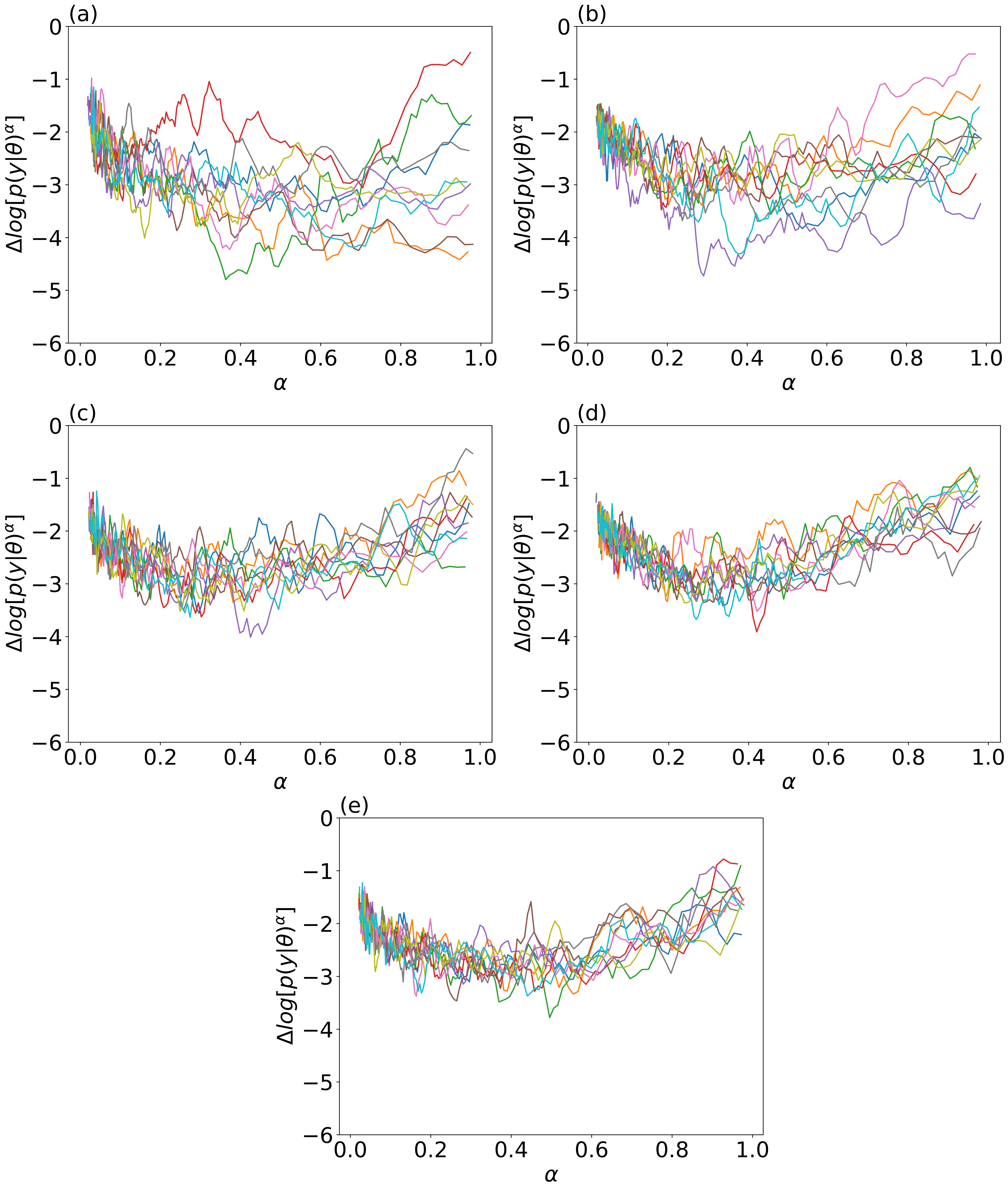
From a computational standpoint, it is beneficial if high-quality uncertainty estimates of the evidences would be obtained from one ASMC run only. Hence, we assess how the predictions of equations 15 and 16 compare with the estimates based on Monte Carlo replications. For smaller , resampling compensates for the faster increasing variance of the weights, but this is at the expense of strong correlations between the particles. The impact of resampling on the variance estimation in equation 15 is primarily embodied in the sum involving the Eve indices. For smaller , more resampling is needed and the number of remaining Eve indices are smaller. Figure 11 illustrates the evolution of the Eve indices for and as the CM1 -sequence progresses. Of the original 40 Eve indices, there are at the end only 3 and 8 Eve indices surviving for and , respectively. For , there are surviving Eve indeces. The larger the number of surviving Eve indices, the less is the risk of mode collapse in which the ASMC algorithm only explore a small part of the posterior distribution. This basically implies that the higher-quality estimates are obtained by using larger or , but this comes at the cost of an increasing number of forward simulations. Table 3 shows the relative standard deviation obtained with Monte Carlo replication and the single ASMC run estimates. For CM1, the relative standard deviations calculated with both estimators are similar for and suggesting that equations 15 and 16 may provide high-quality uncertainty estimates for long-enough ASMC runs. For small , we observe significant underestimation of the relative standard deviations. For , the single ASMC estimation is three times smaller than those obtained by Monte Carlo replication. Why does the single-run ASMC uncertainty estimation work well for large , but not for small ones? To shed some light on this question, we present in Figure 12 the evolution of the difference between the weighted mean of the particles’ likelihoods and the target log-likelihood calculated with the noise realization , both raised to the power of the corresponding with the differences expressed in logarithmic units, that is, . This difference is shown for the ten replications and for the different -values considered. In addition, Table 3 shows the variance and the root-mean-square error (RMSE) for the last states () that decrease with increasing . We observe in Figure 12 that when decreases, the trajectories becomes more separate and show more auto-correlation. At and for which the single-ASMC estimates worked well, we observe that the trajectories overlap and cross each other, thereby, suggesting that the information content of one individual ASMC run is not so much different than another. In contrast, for (Figure 12a) the mean trajectories tend to be more separated from each other suggesting that they sample slightly different posteriors. The Monte Carlo replications account for these differences between individual ASMC runs, while this is impossible when considering estimates from a single ASMC run. This suggests then that the single-run evidence estimator should only be trusted when performing a sufficient number of iterations, thereby, ensuring that the approximations of the intermediate distributions for different ASMC runs are small. In practice, this suggests that it is useful to run at least two ASMC runs and to ensure that the weighted mean-likelihoods of their particles are similar and tend to cross multiple times during the ASMC runs. If this is not the case, our results suggest that the uncertainty estimation of the evidence obtained from one ASMC run is too small.
This finding is also supported by the CM2 estimations in Table 3. This is clearly a more challenging conceptual model, where the used for the ASMC runs was three times higher than for CM1. Even if the single-run uncertainty estimations decrease consistently when increasing , the values are too low compared to those of Monte Carlo replication. This suggests that was not large enough to trust the single-run estimator. This is also reflected in the higher variance and the RMSE of the likelihood difference compared to CM1. This suggests that either Monte Carlo replications are needed to obtain an accurate error estimator or should be increased to improve the reliability of the single-run estimator.

| [single run] | [replications] | |||
|---|---|---|---|---|
| CM1 | ||||
| 1 | 0.62 | 1.72 | 1.70 | 2.99 |
| 3 | 0.42 | 0.66 | 1.42 | 1.91 |
| 5 | 0.35 | 0.50 | 0.62 | 1.84 |
| 10 | 0.29 | 0.27 | 0.67 | 1.14 |
| 20 | 0.21 | 0.20 | 0.69 | 1.47 |
| CM2 | ||||
| 5 | 0.47 | 1.92 | 8.45 | 43.34 |
| 10 | 0.40 | 1.56 | 4.16 | 21.59 |
| 20 | 0.38 | 1.02 | 3.66 | 13.89 |
| 40 | 0.36 | 1.52 | 5.06 | 7.70 |
| 60 | 0.33 | 1.22 | 6.36 | 2.46 |
5 Discussion
Our results suggest that ASMC can provide accurate approximations of posterior PDFs for challenging inverse problems for which state-of-the-art adaptive MCMC fails to converge when considering a similar number of forward simulations (Figure 8). Furthermore, ASMC is very well suited for parallel computation, which is less the case for most MCMC methods. A general recommendation for practical applications is that the algorithmic variables and in Algorithm 1 are chosen sufficiently large to ensure that the weighted-mean likelihood of the particles is close to the target likelihood during the ASMC run (Figure 12). Clearly, if the total number of forward simulations are insufficient, the ASMC algorithm fails in sampling posterior realizations of high likelihood for most particles. This leads to an impoverished particle approximation of the posterior PDF as evidenced by few surviving Eve indices (Figure 11) and mode collapse.
A similar argument holds for the evidence estimation. ASMC provides an unbiased estimation, as shown for the high-noise setting example (section 4.5). However, the evidence estimation procedure will only be reliable if the particles approximate the target power posteriors well enough. In addition, too low and lead to frequent resampling that increases the estimation variance. Our results also suggest that error approximations based on single ASMC runs (eqs. 15 and 16) are too optimistic in such settings, but reliable for sufficiently long ASMC runs (Table 3). We also note that the relative standard deviations of the evidence estimates (Figure 10) are several orders of magnitude smaller than the evidences obtained for the consistent and inconsistent prior models (Table 2).
Providing practical recommendations for parameter settings away from easily-recognizable degenerate conditions is challenging. Of course, the larger the the better, as the particle approximation of the parameter space will be improved. Our choice of was dictated by the number of forward runs we could perform in parallel on one compute node, while much larger values are possible on modern computational architectures. An important point is how well the posterior can be described by a weighted average of particles. The complexity of the posterior distribution depends on several factors like the dimension of the parameter space, the physics, the number and type of data, and the experimental design. Consequently, a much larger number of particles might be needed in challenging high-dimensional settings with strong parameter correlations or for problems with multi-modal posterior PDFs. In agreement with Neal, 2001, we recommend distributing the total number of forward runs for each ASMC particle by favouring a large number of intermediate distributions over larger . In practice, we typically first choose a suitably large and then vary . In contrast to , the influence of on the total number of forward simulations is non-linear and difficult to predict before running the algorithm. The trial tests in this study suggest that needs to be larger than , for our considered ranges of , in order to reach the target misfit and build a smooth -sequence. After fixing , one can then first run the ASMC with an initially small before re-running it with a twice as large value. If the difference between the resulting evidence estimates for these two choices of are much smaller than the computed evidences for competing conceptual models, and if the inferred posteriors are similar, then this choice of is probably sufficient. If important differences are observed between the ASMC runs obtained for the different , then one needs to further double , and so on. Finally, the proposal scale needs to be initialized with a high enough value such that the initial acceptance rate is above . After this, the automatic rescaling of this parameter ensures high-quality estimates regardless of the model proposal scheme.
The observed relative insensitivity of the ASMC results to the model proposal type (Figures 4 and 5) is noteworthy, as the MCMC results (Figure 6) are highly sensitive to this choice. CM1 and CM2 present different levels of complexity. For CM1, MCMC-DREAM achieves convergence without difficulty (Fig. 6i), while this is far from being the case for MCMC-Gauss (Figure 6j). For CM2, both MCMC approaches fail (Figures 6k and l), while ASMC-DREAM and ASMC-Gauss perform similarly well for both CM1 and CM2 (Figures 4 and 5). The underlying reason for the success of ASMC and its insensitivity to the proposal mechanism is likely found due to the following factors. On the one hand, the adaptive scaling of the proposals (e.g., Figure 4c) and the tempering (e.g., Figure 4d) allow the particles to more easily move away from local minima, while resampling, on the other hand, gives priority to the high-likelihood regions (e.g., Figure 4h). Clearly, no such tuning of the proposal scale is possible when using MCMC as it violates detailed balance conditions. We stress that the comparisons made herein are with MCMC algorithms running at a unitary temperature, while parallel tempering-based MCMC methods might not have these problems (Sambridge, 2014).
The presented ASMC method share similarities to other approaches for evidence estimation. Nested Sampling (Skilling, 2004) reduces the evidence multidimensional integral to sampling of a one-dimensional integral over prior mass elements, using an increasing constraint on the log-likelihood lower bound. Other methods rely on MCMC sampling using power posteriors. For instance, thermodynamic integration (TIE) (Gelman and Meng, 1998), also called path sampling, reduces the evidence computation to a one-dimensional integral of the expectation of the likelihood over . Zeng et al., 2018 shows that TIE performs better than nested sampling in terms of accuracy and stability. Stepping Stone Sampling (SS) (Xie et al., 2011) also rely on power-posteriors but improves in accuracy compared with TIE by formulating the evidence estimation by the product of ratios of intermediate normalizing constants, that is, similarly to AIS and ASMC. An important practical difference is that SS is often performed in parallel by running multiple MCMC runs targeting different power posteriors (Brunetti et al., 2019). Since each chain starts from the prior, the total computational cost is high, and perhaps more importantly, there is no solution to deal with MCMC chains for close to one that do not converge (as in our MCMC trials with both MCMC-Gauss and MCMC-DREAM for CM2). This latter problem can be circumvented by running the SS algorithm sequentially using a similar tempering sequence as for ASMC. However, the -sequence needs to be pre-defined, while ASMC allows for adaptive tuning. Even if not presented here, we stress that the improvements offered by ASMC over AIS are drastic. Despite extensive testing and tuning of AIS parameters, we were unable to match the performance of ASMC.
6 Conclusions
This study demonstrates that adaptive sequential Monte Carlo (ASMC) is a powerful method to approximate the posterior PDF and estimate the evidence in non-linear geophysical inverse problems. Crosshole GPR examples in which complex geological priors are parameterized through deep generative networks are used for demonstration purposes, but the method is of wide applicability. ASMC is robust with respect to the type of model proposals used and to algorithmic settings, implying a comparatively low user effort required for tuning the algorithm for a given application. ASMC is particularly useful for moderately to strongly non-linear inverse problems and for multi-modal distributions, where targeting the posterior distribution with MCMC algorithms may result in poor convergence. For the considered examples, ASMC outperforms state-of-the-art adaptive MCMC in estimating posterior PDFs. The major advantage of ASMC compared with MCMC in a Bayesian model selection context is that it provides straightforward computation of the evidence. Reliable uncertainty estimation of evidence estimates is possible from single ASMC runs, provided that they are long enough. We hope that this study will stimulate further adaptations of sequential Monte Carlo in a geophysical context, and more specifically, lead researchers to the adaptation of ASMC when confronted with challenging inference problems and model selection tasks.
7 Acknowledgements
This work was supported by the Swiss National Science Foundation (project number: 184574). We are grateful to Prof. Arnaud Doucet (University of Oxford) who provided highly valuable suggestions at an early stage of this research. We also thank Prof. Adam Johansen (University of Warwick) for responding to an inquiry concerning the original ASMC paper. Finally, we would like to thank the editor Juan Carlos Afonso and two anonymous referees for their constructive comments. Our ASMC code and test examples are available in the following GitHub repository: https://github.com/amaya-macarena/ASMC.
References
- Bergen et al., (2019) Bergen, K. J., Johnson, P. A., Maarten, V., and Beroza, G. C. (2019). Machine learning for data-driven discovery in solid earth geoscience. Science, 363(6433).
- Brown and Neal, (1991) Brown, D. and Neal, A. (1991). The analysis of the variance and covariance of products. Biometrics, 47(2):429–444.
- Brunetti et al., (2019) Brunetti, C., Bianchi, M., Pirot, G., and Linde, N. (2019). Hydrogeological model selection among complex spatial priors. Water Resources Research, 55(8):6729–6753.
- Brunetti et al., (2017) Brunetti, C., Linde, N., and Vrugt, J. A. (2017). Bayesian model selection in hydrogeophysics: Application to conceptual subsurface models of the South Oyster Bacterial Transport Site, Virginia, USA. Advances in Water Resources, 102:127–141.
- Chan and Lai, (2013) Chan, H. P. and Lai, T. L. (2013). A general theory of particle filters in hidden markov models and some applications. Ann. Statist., 41(6):2877–2904.
- Curtis and Lomax, (2001) Curtis, A. and Lomax, A. (2001). Prior information, sampling distributions, and the curse of dimensionality. Geophysics, 66(2):372–378.
- Del Moral et al., (2006) Del Moral, P., Doucet, A., and Jasra, A. (2006). Sequential Monte Carlo samplers. Journal of the Royal Statistical Society: Series B (Statistical Methodology), 68(3):411–436.
- Douc and Cappe, (2005) Douc, R. and Cappe, O. (2005). Comparison of resampling schemes for particle filtering. In ISPA 2005. Proceedings of the 4th International Symposium on Image and Signal Processing and Analysis, 2005., pages 64–69.
- Doucet and Johansen, (2011) Doucet, A. and Johansen, A. M. (2011). A tutorial on particle filtering and smoothing: Fifteen years later. The Oxford Handbook of Nonlinear Filtering, 12(656-704):3.
- Doucet and Lee, (2018) Doucet, A. and Lee, A. (2018). Sequential Monte Carlo methods. Handbook of Graphical Models, pages 165–189.
- Earl and Deem, (2005) Earl, D. J. and Deem, M. W. (2005). Parallel tempering: Theory, applications, and new perspectives. Physical Chemistry Chemical Physics, 7(23):3910–3916.
- Gelman and Meng, (1998) Gelman, A. and Meng, X.-L. (1998). Simulating normalizing constants: From importance sampling to bridge sampling to path sampling. Statistical science, pages 163–185.
- Gelman and Rubin, (1992) Gelman, A. and Rubin, D. B. (1992). Inference from iterative simulation using multiple sequences. Statistical Science, 7(4):457–472.
- Goodfellow et al., (2016) Goodfellow, I., Bengio, Y., and Courville, A. (2016). Deep Learning. MIT Press. http://www.deeplearningbook.org.
- Goodfellow et al., (2014) Goodfellow, I., Pouget-Abadie, J., Mirza, M., Xu, B., Warde-Farley, D., Ozair, S., Courville, A., and Bengio, Y. (2014). Generative adversarial nets. In Advances in Neural Information Processing Systems, pages 2672–2680.
- Hammersley and Handscomb, (1964) Hammersley, J. M. and Handscomb, D. C. (1964). General Principles of the Monte Carlo Method, pages 50–75. Springer Netherlands, Dordrecht.
- Hansen et al., (2012) Hansen, T. M., Cordua, K. S., and Mosegaard, K. (2012). Inverse problems with non-trivial priors: efficient solution through sequential Gibbs sampling. Computational Geosciences, 16(3):593–611.
- Jetchev et al., (2016) Jetchev, N., Bergmann, U., and Vollgraf, R. (2016). Texture synthesis with spatial generative adversarial networks. arXiv preprint arXiv:1611.08207.
- Karpatne et al., (2018) Karpatne, A., Ebert-Uphoff, I., Ravela, S., Babaie, H. A., and Kumar, V. (2018). Machine learning for the geosciences: Challenges and opportunities. IEEE Transactions on Knowledge and Data Engineering, 31(8):1544–1554.
- Kingma and Welling, (2013) Kingma, D. P. and Welling, M. (2013). Auto-encoding variational Bayes. arXiv preprint arXiv:1312.6114.
- Kirkpatrick et al., (1983) Kirkpatrick, S., Gelatt, C. D., and Vecchi, M. P. (1983). Optimization by simulated annealing. Science, 220(4598):671–680.
- Koltermann and Gorelick, (1996) Koltermann, C. E. and Gorelick, S. M. (1996). Heterogeneity in sedimentary deposits: A review of structure-imitating, process-imitating, and descriptive approaches. Water Resources Research, 32(9):2617–2658.
- Kong et al., (1994) Kong, A., Liu, J. S., and Wong, W. H. (1994). Sequential imputations and Bayesian missing data problems. Journal of the American Statistical Association, 89(425):278–288.
- Laloy et al., (2018) Laloy, E., Hérault, R., Jacques, D., and Linde, N. (2018). Training-image based geostatistical inversion using a spatial generative adversarial neural network. Water Resources Research, 54(1):381–406.
- Laloy et al., (2017) Laloy, E., Hérault, R., Lee, J., Jacques, D., and Linde, N. (2017). Inversion using a new low-dimensional representation of complex binary geological media based on a deep neural network. Advances in Water Resources, 110:387–405.
- Laloy et al., (2019) Laloy, E., Linde, N., Ruffino, C., Hérault, R., Gasso, G., and Jacques, D. (2019). Gradient-based deterministic inversion of geophysical data with generative adversarial networks: Is it feasible? Computers & Geosciences, 133:104333.
- Laloy and Vrugt, (2012) Laloy, E. and Vrugt, J. A. (2012). High-dimensional posterior exploration of hydrologic models using multiple-try DREAM(ZS) and high-performance computing. Water Resources Research, 48(1).
- LeCun et al., (2015) LeCun, Y., Bengio, Y., and Hinton, G. (2015). Deep learning. nature, 521(7553):436–444.
- Lee and Whiteley, (2018) Lee, A. and Whiteley, N. (2018). Variance estimation in the particle filter. Biometrika, 105(3):609–625.
- Lewis and Raftery, (1997) Lewis, S. M. and Raftery, A. E. (1997). Estimating Bayes factors via posterior simulation with the Laplace—Metropolis estimator. Journal of the American Statistical Association, 92(438):648–655.
- Linde et al., (2017) Linde, N., Ginsbourger, D., Irving, J., Nobile, F., and Doucet, A. (2017). On uncertainty quantification in hydrogeology and hydrogeophysics. Advances in Water Resources, 110:166–181.
- Linde et al., (2015) Linde, N., Renard, P., Mukerji, T., and Caers, J. (2015). Geological realism in hydrogeological and geophysical inverse modeling: A review. Advances in Water Resources, 86:86–101.
- Mariethoz and Caers, (2014) Mariethoz, G. and Caers, J. (2014). Multiple-point geostatistics: Stochastic modeling with training images. John Wiley & Sons.
- Mariethoz et al., (2010) Mariethoz, G., Renard, P., and Caers, J. (2010). Bayesian inverse problem and optimization with iterative spatial resampling. Water Resources Research, 46(11).
- Mosegaard and Tarantola, (1995) Mosegaard, K. and Tarantola, A. (1995). Monte carlo sampling of solutions to inverse problems. Journal of Geophysical Research: Solid Earth, 100(B7):12431–12447.
- Mosser et al., (2017) Mosser, L., Dubrule, O., and Blunt, M. J. (2017). Reconstruction of three-dimensional porous media using generative adversarial neural networks. Physical Review E, 96(4):043309.
- Mosser et al., (2020) Mosser, L., Dubrule, O., and Blunt, M. J. (2020). Stochastic seismic waveform inversion using generative adversarial networks as a geological prior. Mathematical Geosciences, 52(1):53–79.
- Neal, (2001) Neal, R. M. (2001). Annealed importance sampling. Statistics and Computing, 11(2):125–139.
- Peterson, (2001) Peterson, Jr, J. E. (2001). Pre-inversion corrections and analysis of radar tomographic data. Journal of Environmental & Engineering Geophysics, 6(1):1–18.
- Pirot et al., (2019) Pirot, G., Huber, E., Irving, J., and Linde, N. (2019). Reduction of conceptual model uncertainty using ground-penetrating radar profiles: Field-demonstration for a braided-river aquifer. Journal of Hydrology, 571:254–264.
- Pirot et al., (2015) Pirot, G., Straubhaar, J., and Renard, P. (2015). A pseudo genetic model of coarse braided-river deposits. Water Resources Research, 51(12):9595–9611.
- Podvin and Lecomte, (1991) Podvin, P. and Lecomte, I. (1991). Finite difference computation of traveltimes in very contrasted velocity models: a massively parallel approach and its associated tools. Geophysical Journal International, 105(1):271–284.
- Renard and Allard, (2013) Renard, P. and Allard, D. (2013). Connectivity metrics for subsurface flow and transport. Advances in Water Resources, 51:168–196.
- Roth et al., (1990) Roth, K., Schulin, R., Flühler, H., and Attinger, W. (1990). Calibration of time domain reflectometry for water content measurement using a composite dielectric approach. Water Resources Research, 26(10):2267–2273.
- Sambridge, (2014) Sambridge, M. (2014). A parallel tempering algorithm for probabilistic sampling and multimodal optimization. Geophysical Journal International, 196(1):357–374.
- Schöniger et al., (2014) Schöniger, A., Wöhling, T., Samaniego, L., and Nowak, W. (2014). Model selection on solid ground: Rigorous comparison of nine ways to evaluate Bayesian model evidence. Water Resources Research, 50(12):9484–9513.
- Scott, (2015) Scott, D. W. (2015). Multivariate Density Estimation: Theory, Practice, and Visualization. John Wiley & Sons.
- Skilling, (2004) Skilling, J. (2004). Nested sampling. In AIP Conference Proceedings, volume 735, pages 395–405. American Institute of Physics.
- Vrugt, (2016) Vrugt, J. A. (2016). Markov chain Monte Carlo simulation using the DREAM software package: Theory, concepts, and MATLAB implementation. Environmental Modelling & Software, 75:273–316.
- Xie et al., (2011) Xie, W., Lewis, P. O., Fan, Y., Kuo, L., and Chen, M.-H. (2011). Improving marginal likelihood estimation for Bayesian phylogenetic model selection. Systematic Biology, 60(2):150–160.
- Zahner et al., (2016) Zahner, T., Lochbühler, T., Mariethoz, G., and Linde, N. (2016). Image synthesis with graph cuts: a fast model proposal mechanism in probabilistic inversion. Geophysical Journal International, 204(2):1179–1190.
- Zeng et al., (2018) Zeng, X., Ye, M., Wu, J., Wang, D., and Zhu, X. (2018). Improved nested sampling and surrogate-enabled comparison with other marginal likelihood estimators. Water Resources Research, 54(2):797–826.
- Zhou et al., (2016) Zhou, Y., Johansen, A. M., and Aston, J. A. (2016). Toward automatic model comparison: an adaptive sequential Monte Carlo approach. Journal of Computational and Graphical Statistics, 25(3):701–726.