marginparsep has been altered.
topmargin has been altered.
marginparwidth has been altered.
marginparpush has been altered.
The page layout violates the ICML style.
Please do not change the page layout, or include packages like geometry, savetrees, or fullpage, which change it for you.
We’re not able to reliably undo arbitrary changes to the style. Please remove the offending package(s), or layout-changing commands and try again.
Modulating Regularization Frequency
for Efficient Compression-Aware Model Training
Dongsoo Lee * 1 Se Jung Kwon * 1 Byeongwook Kim * 1 Jeongin Yun 1 Baeseong Park 1 Yongkweon Jeon 1
Abstract
While model compression is increasingly important because of large neural network size, compression-aware training is challenging as it needs sophisticated model modifications and longer training time. In this paper, we introduce regularization frequency (i.e., how often compression is performed during training) as a new regularization technique for a practical and efficient compression-aware training method. For various regularization techniques, such as weight decay and dropout, optimizing the regularization strength is crucial to improve generalization in Deep Neural Networks (DNNs). While model compression also demands the right amount of regularization, the regularization strength incurred by model compression has been controlled only by compression ratio. Throughout various experiments, we show that regularization frequency critically affects the regularization strength of model compression. Combining regularization frequency and compression ratio, the amount of weight updates by model compression per mini-batch can be optimized to achieve the best model accuracy. Modulating regularization frequency is implemented by occasional model compression while conventional compression-aware training is usually performed for every mini-batch.
1 Introduction
Weight regularization is a process adding information to the model to avoid overfitting Goodfellow et al. 2016; van Laarhoven 2017. In this paper, we explore weight compression as a form of weight regularization as it severely restricts the search space of weights (i.e., regularized by compression forms). Moreover, model compression shrinks the effective model size, which is an important regularization principle Goodfellow et al. 2016 (note that improved model accuracy by model compression is reported Frankle et al. 2019). Weights are regularized in numerous ways by model compression. For example, each weight can be pruned (e.g., Han et al. 2015) or quantized (e.g., Guo et al. 2017) to yield a sparse model representation or to reduce the number of bits to represent each weight.
While model compression can be performed without training dataset, compression-aware training can improve model accuracy by reflecting the impact of model compression on the loss function for every mini-batch update Courbariaux et al. 2015; Zhu & Gupta 2017; Zhu et al. 2017; Guo et al. 2017. For such a method, the regularization strength is mainly determined by compression ratio. Note that for typical regularization schemes, adjusting the regularization strength, such as dropout rate or weight decay factor, is a crucial process to maximize generalization capability of DNNs. To improve model accuracy given a target compression ratio, we need an additional way to control the regularization strength.
In this paper, we introduce regularization frequency to represent how many mini-batches are trained without regularization. Then for weight decay and weight noise insertion, we show that decreasing regularization frequency allows higher weight decay factors or larger amounts of noise per regularization step. In other words, the overall regularization strength is affected by regularization frequency as well as weight decay factors (or the amount of weight noise). As a result, a similar amount of average weight updates (determined by both regularization frequency and weight decay factors) is associated with a similar regularization strength, and hence, similar model accuracy. We demonstrate that the same principle holds for model compression; regularization strength is affected not only by compression ratio but also by regularization frequency. We verify that our simple model compression techniques (without modifying the underlying training procedures) based on occasional weight regularization can achieve higher compression ratio and higher model accuracy compared to previous techniques that demand substantial modifications to the training process.
Our proposed compression-aware training algorithm enables the followings:
- •
Our compression-aware training technique does not require any modifications to the original training algorithms except an additional regularization method in that weights are occasionally transformed by compression forms.
- •
Computational overhead by compression is not noticeable because such new additional regularization is performed infrequently. Hence, complex compression algorithms are allowed without concerns on training time increase.
- •
We propose an additional regularization hyper-parameter, regularization frequency, to provide larger parameter search space.
- •
Our proposed training method can be a platform to support various kinds of compression techniques including even futuristic ones. Model compression designers can focus on developing new compression architectures without concerns on particular associated training algorithm design.
2 Batch Size Selection
Since a unit of measurement of regularization frequency is highly correlated with batch size, let us discuss batch size considered for our work. To overcome some practical issues of gradient descent on non-convex optimization problems, there have been several enhancements such as learning rate scheduling and adaptive update schemes using momentum and update history Ruder 2016. Optimizing batch size is another way to yield efficient gradient descent. Note that large batch size has the advantage of enhancing parallelism of the training system in order to speed up training, critical for DNN research Dean et al. 2012. Despite such advantages, small batch size is preferred because it improves generalization associated with flat minima search Keskar et al. 2016 and other hyper-parameter explorations are more convenient Masters & Luschi 2018. Small batch size also affects weight regularization if weight updates for gradient descent and weight regularization are supposed to happen for every mini-batch. For example, for weight decay conducted for every mini-batch, if batch size is modified, then the weight decay factor should also be adjusted accordingly Loshchilov & Hutter 2017. In this paper, we assume a reasonably small batch size.
3 Weight Updates by Model Compression

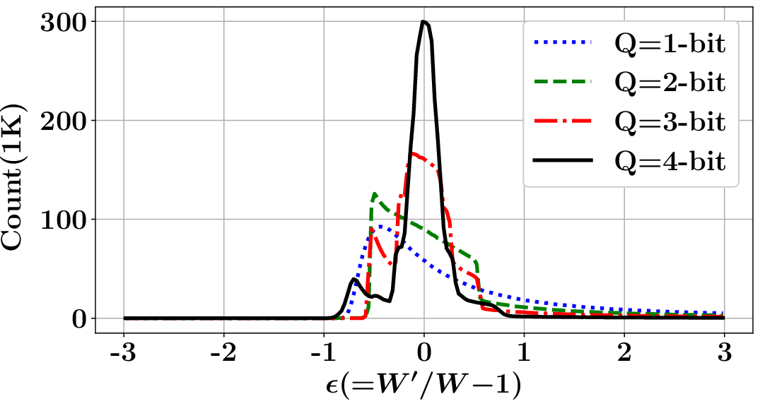
Before investigating the effects of regularization frequency, we first study the relationship between model compression ratio and the weight regularization strength using quantization and singular-value decomposition (SVD) as model compression techniques. We assume a popular quantization method based on binary codes for which a weight vector is approximated to be for -bit quantization, where is a scaling factor and is a binary vector, and is the vector size. The quantization error is minimized by a method proposed by Xu et al. 2018 to compute and . For SVD, a weight matrix is approximated to be by minimizing subject to rank, where is the target rank.
For our experiments, we use a synthetic ) weight matrix where each element is randomly generated from the Gaussian distribution . Then, we are interested in the amount of change of each weight after quantization and SVD. Assuming that weight noise through compression is expressed as in the form of , Figure 1 shows the distribution of with various quantization bits or target ranks. From distributions skewed to be negative, it is clear that weights tend to decay more with higher compression ratio, along with a wider range of random noise. Reasonable explanations of Figure 1 would include: 1) weights generated from the Gaussian distribution are uncorrelated such that an approximation step (by compression) using multiple weights would result in noise for each weight, 2) in the case of SVD, elements associated with small eigenvalues are eliminated, 3) averaging effects in quantization reduce the magnitude of large weights. For weight pruning, becomes or (i.e., weight decay for selected weights). Correspondingly, we study weight decay and weight noise insertion in the next two sections as an effort to gain a part of basic knowledge on improved training for model compression, even though actual model compression would demand much more complicated weight noise models.

4 Non-Regularization Period Study on Weight Decay and Weight Noise Insertion
Since weight regularization cannot precede updates for gradient descent, in order to control the frequency of weight regularization, an available option is to skip a few batches without regularization. In this paper, we propose a new hyper-parameter, called “Non-Regularization period” or NR period, to enable occasional regularization and to define the interval of two consecutive regularization events as shown in Figure 2. NR period is an integer number and expressed as a multiple of batches (from now on, thus, we use ‘NR period’ or to represent regularization frequency).
Weight decay is one of the most well-known regularization techniques Zhang et al. 2018 and different from regularization in a sense that weight decay is separated from the loss function calculation Loshchilov & Hutter 2017. Weight decay is performed as
| (1) |
where is a constant weight decay factor. Weight noise insertion is another regularization technique aiming at reaching flat minima Goodfellow et al. 2016; Hochreiter & Schmidhuber 1995. For our experiments, we assume that random Gaussian noise is added to weights such that when .


We study the impact of NR period on weight decay and weight noise insertion using ResNet-32 on CIFAR-10 model He et al. 2016 and a long short-term memory (LSTM) model on PTB dataset Zaremba et al. 2014. For the LSTM model, we use 2 layers with 200 hidden units and the hyper-parameter set introduced by Zaremba et al. 2014. For the weight noise model, we plug (uniform distribution) into Eq. (6) to simplify the experiments. Figure 3 shows model accuracy of ResNet-32 given different NR period and weight decay factors. For both weight decay and weight noise insertion, the choice of (representing the amount of weight regularization for every ) has a clear correlation with NR period (refer to Appendix for training and test accuracy graphs). If we wish to apply larger , then weight regularization should be conducted less frequently (i.e., larger weight decay factor requires longer NR period) to optimize the regularization effect and achieve high model accuracy. For similar model accuracy, weight decay factor can be approximately 1,000 times larger with in Figure 3 and Figure 4. Similar observations are discovered by the LSTM model on PTB as shown in Figure 4. Lower perplexity (indicating better generalization) is obtained when the NR period increases as becomes larger for each regularization event. For weight decay, increasing by longer may not be significant because of similar model accuracy. On the other hand, increasing model compression ratio by longer should be significant as we show in the next section.
5 NR Period for Model Compression
As discussed, weight compression incurs a much more complicated weight regularization model than weight decay or uniform weight noise insertion because 1) as shown in Figure 1, diversified noise models need to be combined to describe weight regularization after model compression and 2) compression-aware training methods would reduce the strength of weight regularization as training is performed with more epochs and weights converge to a compressed form. Nonetheless, we can conjecture that the best training scheme for model compression may require the condition of that can be empirically justified.


We apply weight quantization, low-rank approximation (SVD), and pruning to an LSTM model on PTB that we selected for the previous section. We do not modify underlying training principles and use the following simple strategy:
(1)
Train the model for batches
(as if model compression is not being considered.)
(2)
Perform weight compression in the form of
.
(3)
With new full-precision weight ,
repeat the above two steps.
can be a magnitude-based pruning (i.e., = if is larger than a certain threshold, or =, otherwise), for quantization, SVD function, or even as-yet undiscovered functions.
Figure 5 shows model accuracy associated with a number of different sets of and model compression strength (i.e., target rank for low-rank approximation and the number of quantization bits). Notice that the optimal for the best model accuracy is definitely larger than . To explain how Figure 5 is aligned with the previous section, we investigate the relationship between model accuracy and the average of (, where is a weight vector after weight decay, SVD, or pruning) throughout the entire training. We first optimize to achieve the best model accuracy. Following Figure 3 and 4, let us assume to be constant regardless of compression ratio or decay factor, and obtained by finding hyper-parameter sets associated with maximum model accuracy in Figure 4 and Figure 5 and by taking the average of corresponding values. When regularization error is defined to be , Figure 6 shows test perplexity and regularization error of PTB LSTM model with different . Such defined regularization error is affected by as shown in Figure 6, and indeed, when regularization error approaches to the minimum (i.e., zero) we gain improved model accuracy. Unlike weight decay where is directly computed by decay factors, for model compression techniques, is not directly related to compression-related hyper-parameters (such as ranks and pruning rates). As a result, while Figure 4 shows a clear correlation between decay factors and for best model accuracy, Figure 5 suggests that compression ratio and are weakly correlated. Hence, is a hyper-parameter to be determined empirically for model compression. Nonetheless, the optimal is definitely larger than 1, as shown in Figure 6, and decoupled from batch size selection. That means weight regularization for model compression needs to be conducted much less frequently compared with gradient descent since batch size selection considers generalization ability of gradient descent, not regularization effects.
For ResNet-32 on CIFAR-10, we also find and investigate the relationship between model accuracy and as shown in Figure 7. Similar to the case of PTB LSTM model, ResNet-32 presents a particular that minimizes regularization error. It is clear that for both PTB LSTM and ResNet-32, optimal is definitely larger than ‘1’ despite some variation on model accuracy. We summarize our empirical observations as follows:
- •
Unlike conventional wisdom, a wide range of weight decay factors is allowed since we can adjust to optimize the regularization strength.
- •
For each weight decay factor selected, there is an optimal to maximize model accuracy.
- •
Similarly, for each compression ratio, a particular presents the best model accuracy.
- •
Such is a hyper-parameter that is empirically searched.
From our extensive experiments, optimal is usually searched in the range from 10 to 1000 for model compression. Large provides a benefit of less amount computations for model compression. Especially when the compression method is based on iterative mathematical principles (such as SVD N. Sainath et al. 2013 or quantization Xu et al. 2018), large can save training time significantly.
6 Comparison with Previous Model Compression Techniques
In this section, we compare some of previous model compression techniques with our compression scheme that introduces and obviates special training algorithm modifications. Due to the space limit, please refer to Appendix for more experimental results with ImageNet and PTB.
6.1 Fine-Grained Weight Pruning
The initial attempt of pruning weights was to locate redundant weights by computing the Hessian to calculate the sensitivity of weights to the loss function LeCun et al. 1990. However, such a technique has not been considered to be practical due to significant computation overhead for computing the Hessian. Magnitude-based pruning Han et al. 2015 has become popular because one can quickly find redundant weights by simply measuring the magnitude of weights. Since then, numerous researchers have realized a higher compression ratio largely by introducing Bayesian inference modeling of weights accompanying supplementary hyper-parameters. For example, dynamic network surgery (DNS) Guo et al. 2016 permits weight splicing when a separately stored full-precision weight becomes larger than a certain threshold. Optimizing splicing threshold values, however, necessitates extensive search space exploration, and thus, longer training time. Variational dropout method Molchanov et al. 2017 introduces an explicit Bayesian inference model for a prior distribution of weights, which also induces various hyper-parameters and increased computational complexity.
We perform magnitude-based pruning at every step. As a result, even though weights are pruned and replaced with zero at steps, pruned weights are still updated in full precision during NR period. If the amount of updates of a pruned weight grows large enough between two consecutive regularization steps, then the weight pruned at the last step may not be pruned at the next step. Such a feature (i.e., pruning decisions are not fixed) is also utilized for weight splicing in DNS Guo et al. 2016. Weight splicing in DNS relies on a hysteresis function (demanding sophisticated fine-tuning process with associated hyper-parameters) to switch pruning decisions. Pruning decisions through our scheme, on the other hand, are newly determined at every step.
We present experimental results with LeNet-5 and LeNet-300-100 models on MNIST dataset which are also reported by Guo et al. 2016; Molchanov et al. 2017. LeNet-5 consists of 2 convolutional layers and 2 fully connected layers while 3 fully connected layers construct LeNet-300-100. We train both models for 20000 steps using Adam optimizer where batch size is 50. All the layers are pruned at the same time and the pruning rate increases gradually Zhu & Gupta 2017. We exclude dropout to improve the accuracy of LeNet-300-100 and LeNet-5 since pruning already works as a regularizer Han et al. 2015; Wan et al. 2013. We keep the original learning schedule and the total number of training steps (no additional training time for model compression).
| Model | Layer | Weight | Pruning Rate (%) | |||
| Size | DC | DNS | SparseVD | Ours | ||
| FC1 | 235K | 92 | 98.2 | 98.9 | 98.9 | |
| LeNet | FC2 | 30K | 91 | 98.2 | 97.2 | 96.0 |
| -300-100 | FC3 | 1K | 74 | 94.5 | 62.0 | 62.0 |
| Total | 266.2K | 92 | 98.2 | 98.6 | 98.4 | |
| LeNet-5 | Conv1 | 0.5K | 34 | 85.8 | 67 | 60.0 |
| Conv2 | 25K | 88 | 96.9 | 98 | 97.0 | |
| FC1 | 40K | 92 | 99.3 | 99.8 | 99.8 | |
| FC2 | 5K | 81 | 95.7 | 95 | 95.0 | |
| Total | 430K | 92 | 99.1 | 99.6 | 99.5 | |
| Model | Accuracy (%) | |||
| DC | DNS | Sparse VD | DeepTwist | |
| LeNet-300-100 | 98.4 | 98.0 | 98.1 | 98.1 |
| LeNet-5 | 99.2 | 99.1 | 99.2 | 99.1 |
| NR Period () | 1 | 2 | 5 | 10 | 50 | 100 | 200 | 500 |
| Accuracy (%) | 99.00 | 99.06 | 99.06 | 99.11 | 99.05 | 98.98 | 98.72 | 96.52 |
Table 1 presents the comparison on pruning rates (see Appendix for test accuracy that is almost the same among all selected schemes). Despite the simplicity, our pruning scheme produces higher pruning rate compared with DNS and similar compared with variational dropout technique which involves much higher computational complexity. For Table 1, we use =10 for LeNet-5 and =5 for LeNet-300-100.
We investigate how sensitive is to the test accuracy when the other parameters (such as pruning rates, learning rate, and total training time) are fixed. As shown in Table 2, for a wide range of , the test accuracy has negligible fluctuation11 1 Even though we cannot show such a sensitivity study for all of the remaining experiments in this paper, has also shown low sensitivity to the accuracy even for other models and compression techniques.. Too large would result in 1) too little weight distortion, 2) coarse-grained gradual pruning, and 3) unnecessarily large updates for correctly pruned weights. On the other hand, too small may yield excessive amounts of weight distortion and reduce the opportunity for the pruned weights to recover.
We apply -based pruning to an RNN model to verify the effectiveness of . We choose an LSTM model (Zaremba et al. 2014) on the PTB dataset (Marcus et al. 1993). Following the model structure given in Zaremba et al. 2014, our model consists of an embedding layer, 2 LSTM layers, and a softmax layer. The number of LSTM units in a layer can be 200, 650, or 1500, depending on the model configurations (referred as small, medium, and large model, respectively). The accuracy is measured by Perplexity Per Word (PPW), denoted simply by perplexity in this paper. -based pruning for the PTB models is performed gradually using and the initial learning rate is 2.0 for the medium model (1.0 for pre-training) and 1.0 for the large model (1.0 for pre-training) while the learning policy remains to be the same as in Zaremba et al. 2014.
| Model Size | Pruning Method | Perplexity | ||||||
| = | 0% | 80% | 85% | 90% | 95% | 97.5% | ||
| Medium | (Zhu & Gupta 2017) | 83.37 | 83.87 | 85.17 | 87.86 | 96.30 | 113.6 | |
| (19.8M) | DeepTwist | 83.78 | 81.54 | 82.62 | 84.64 | 93.39 | 110.4 | |
| Large | (Zhu & Gupta 2017) | 78.45 | 77.52 | 78.31 | 80.24 | 87.83 | 103.20 | |
| (66M) | DeepTwist | 78.07 | 77.39 | 77.73 | 78.28 | 84.69 | 99.69 | |


For all of the pruning rates selected, Table 3 shows that our compression scheme improves perplexity better than the technique in Zhu & Gupta 2017 which is based on Han et al. 2015. The superiority of -based pruning is partly supported by the observation that non-zero weights successfully avoid to be small through retraining while the conventional pruning still keeps near-zero (unmasked) weights as depicted in Figure 8.
6.2 Low-Rank Approximation
We apply our proposed occasional regularization algorithm integrated with Tucker decomposition Tucker 1966 to convolutional neural network (CNN) models and demonstrate superiority of the -based scheme over conventional training methods. In CNNs, the convolution operation requires a 4D kernel tensor where each kernel has dimension, is the input feature map size, and is the output feature map size. Then, following the Tucker decomposition algorithm, is decomposed into three components as
| (2) |
where is the reduced kernel tensor, is the rank for input feature map dimension, is the rank for output feature map dimension, and and are 2D filter matrices to map to . As a result, one convolution layer is divided into three convolution layers, specifically, convolution for , convolution for , and convolution for Kim et al. 2016.
In prior tensor decomposition schemes, model training is performed as a fine-tuning procedure after the model is restructured and fixed Lebedev et al. 2015; Kim et al. 2016. On the other hand, our training algorithm is conducted for Tucker decomposition as follows:
- 1.
Perform normal training for (batches) without considering Tucker decomposition
- 2.
Calculate , , and using Tucker decomposition to obtain
- 3.
Replace with
- 4.
Go to Step 1 with updated
After repeating a number of the above steps towards convergence, the entire training process should stop at Step 2, and then the final decomposed structure is extracted for inference. Because the model is not restructured except in the last step, Steps 2 and 3 can be regarded as special steps to encourage wide search space exploration so as to find a compression-friendly local minimum where weight noise by decomposition does not noticeably degrade the loss function.
Using the pre-trained ResNet-32 model with CIFAR-10 dataset He et al. 2016; Kossaifi et al. 2019, we compare two training methods for Tucker decomposition: 1) typical training with a decomposed model and 2) -based training, which maintains the original model structure and occasionally injects weight noise through decomposition. Using an SGD optimizer, both training methods follow the same learning schedule: learning rate is 0.1 for the first 100 epochs, 0.01 for the next 50 epochs, and 0.001 for the last 50 epochs. Except for the first layer, which is much smaller than the other layers, all convolution layers are compressed by Tucker decomposition with rank and selected to be and multiplied by a constant number ( in this experiment). Then, the compression ratio of a convolution layer is , which can be approximated to be if and . is chosen to be 200.


Figure 9 shows test accuracy after Tucker decomposition22 2 https://github.com/larry0123du/Decompose-CNN by two different training methods. Note that test accuracy results are evaluated only at Step 3 where the training process can stop to generate a decomposed structure. In Figure 9, across a wide range of compression ratios (determined by ), the proposed scheme yields higher model accuracy compared to typical training. Note that even higher model accuracy than that of the pre-trained model can be achieved by our method if the compression ratio is small enough. In fact, Figure 10 shows that our technique improves training loss and test accuracy throughout the entire training process. Initially, the gap of training loss and test accuracy between pre-regularization and post-regularization is large. Such a gap, however, is quickly reduced through training epochs. Overall, ResNet-32 converges successfully through the entire training process with lower training loss and higher test accuracy compared with a typical training method.
To investigate the effect of NR period on local minima exploration with ResNet-32 on CIFAR-10, Figure 11 presents the changes of loss function and weight magnitude values incurred by occasional regularization. In Figure 11(left), is given as the loss function increase (due to weight regularization at steps) divided by , which is the loss function value right before weight regularization. In Figure 11(right), is defined as , where is the entire set of weights to be compressed, is the set of weights regularized by Tucker decomposition, is the number of elements of , and is the Frobenius norm of . Initially, fluctuates with large corresponding . Then, both and decrease and Figure 11 shows that occasional regularization finds flatter local minima (in the view of Tucker decomposition) successfully. When the learning rate is reduced at 100th and 150th epochs, and decrease significantly because of a lot reduced local minima exploration space. In other words, occasional regularization helps an optimizer to detect a local minimum where Tucker decomposition does not alter the loss function value noticeably.

For ResNet-18 on ImageNet experiments and VGG19 on CIFAR-10 (including additional compression techniques), refer to Appendix.
7 NR Period for Convergence

NR period influences convergence in training. Strong weight regularization facilitates the chance of escaping a local minimum (depicted as step 2 in Figure 12) or requires longer NR period to return to a local minimum (described as step 5 in Figure 12). Let us estimate the desirable NR period () considering the convergence of training even though is supposed to be searched empirically. Given a parameter set (that is assumed to be close enough to a local minimum) and a learning rate , the loss function of a model can be approximated as
| (3) |
using a local quadratic approximation where is the Hessian of and is a set of parameters at a local minimum. After regularization is performed at step , can be updated by gradient descent as follows:
| (4) |
Thus, after , we obtain
| (5) |
where is an identity matrix. Suppose that is positive semi-definite and all elements of are less than 1.0, can converge to with long which should be longer with larger (i.e., stronger weight regularization) or smaller .
8 Related Work
Periodic compression has been introduced in the literature to gradually improve compression ratio or automate hyper-parameter search process. DropPruning repeats dropping weights randomly and retraining the model while some previously dropped weights are unpruned until pruning rate reaches a target number Jia et al. 2018. Weights are incrementally quantized to improve model accuracy Zhou et al. 2017 or the number of quantization bits can be controlled differently for each layer by a loop based on reinforcement learning Elthakeb et al. 2018. Structured pruning and fine-tuning process can be iterated to increase pruning rate Molchanov et al. 2016; Liu et al. 2017. All of these previous works assume (i.e., performing compression for every mini batch) while the goal is increasing compression ratio slowly or finding a set of hyper-parameters through iterative fine-tuning stages. Our proposed compression technique can be combined with such periodic compression methods (incremental compression or automatic hyper-parameter selection are also applicable to our proposed method). In the work by He et al. 2018, soft filter pruning is conducted with = 1 epoch without analysis of why such occasional pruning improves model accuracy.
9 Conclusion
In this paper, we introduce a new hyper-parameter called non-regularization period or NR period during which weights are updated only for gradient computations. NR period (or equivalently regularization frequency) provides a critical impact on the overall regularization strength. For example, if a weight decay factor becomes larger, then NR period can be longer to maintain the regularization strength. Using such a property, we demonstrate that during compression-aware training, NR period can control the regularization strength given a target compression ratio such that model accuracy is improved compared to the case of compression for every mini-batch. Throughout various experiments, we show that there is a particular NR period (associated with occasional weight compression accordingly) that maximizes model accuracy.
References
- Chetlur et al. (2014) Chetlur, S., Woolley, C., Vandermersch, P., Cohen, J., Tran, J., Catanzaro, B., and Shelhamer, E. cuDNN: Efficient primitives for deep learning. arXiv:1410.0759, 2014.
- Cho & Brand (2017) Cho, M. and Brand, D. MEC: memory-efficient convolution for deep neural network. In International Conference on Machine Learning (ICML), pp. 815–824, 2017.
- Courbariaux et al. (2015) Courbariaux, M., Bengio, Y., and David, J.-P. BinaryConnect: Training deep neural networks with binary weights during propagations. In Advances in Neural Information Processing Systems, pp. 3123–3131, 2015.
- Dean et al. (2012) Dean, J., Corrado, G., Monga, R., Chen, K., Devin, M., Mao, M., aurelio Ranzato, M., Senior, A., Tucker, P., Yang, K., Le, Q. V., and Ng, A. Y. Large scale distributed deep networks. In Advances in Neural Information Processing Systems, pp. 1223–1231, 2012.
- Elthakeb et al. (2018) Elthakeb, A. T., Pilligundla, P., Yazdanbakhsh, A., Kinzer, S., and Esmaeilzadeh, H. Releq: A reinforcement learning approach for deep quantization of neural networks. arXiv preprint arXiv:1811.01704, 2018.
- Fatahalian et al. (2004) Fatahalian, K., Sugerman, J., and Hanrahan, P. Understanding the efficiency of GPU algorithms for matrix-matrix multiplication. In Proceedings of the ACM SIGGRAPH/EUROGRAPHICS Conference on Graphics Hardware, pp. 133–137, 2004.
- Frankle et al. (2019) Frankle, J., Dziugaite, G. K., Roy, D. M., and Carbin, M. Stabilizing the lottery ticket hypothesis. arXiv:1903.01611, 2019.
- Goodfellow et al. (2016) Goodfellow, I., Bengio, Y., and Courville, A. Deep Learning. MIT Press, 2016. http://www.deeplearningbook.org.
- Guo et al. (2016) Guo, Y., Yao, A., and Chen, Y. Dynamic network surgery for efficient DNNs. In Advances in Neural Information Processing Systems, 2016.
- Guo et al. (2017) Guo, Y., Yao, A., Zhao, H., and Chen, Y. Network sketching: exploiting binary structure in deep CNNs. In IEEE Conference on Computer Vision and Pattern Recognition (CVPR), pp. 4040–4048, 2017.
- Han et al. (2015) Han, S., Pool, J., Tran, J., and Dally, W. J. Learning both weights and connections for efficient neural networks. In Advances in Neural Information Processing Systems, pp. 1135–1143, 2015.
- Han et al. (2016) Han, S., Mao, H., and Dally, W. J. Deep compression: Compressing deep neural networks with pruning, trained quantization and Huffman coding. In International Conference on Learning Representations (ICLR), 2016.
- He et al. (2016) He, K., Zhang, X., Ren, S., and Sun, J. Deep residual learning for image recognition. 2016 IEEE Conference on Computer Vision and Pattern Recognition (CVPR), pp. 770–778, 2016.
- He et al. (2018) He, Y., Kang, G., Dong, X., Fu, Y., and Yang, Y. Soft filter pruning for accelerating deep convolutional neural networks. arXiv preprint arXiv:1808.06866, 2018.
- Hochreiter & Schmidhuber (1995) Hochreiter, S. and Schmidhuber, J. Simplifying neural nets by discovering flat minima. In Advances in Neural Information Processing Systems, pp. 529–536, 1995.
- Jia et al. (2018) Jia, H., Xiang, X., Fan, D., Huang, M., Sun, C., Meng, Q., He, Y., and Chen, C. Droppruning for model compression. arXiv preprint arXiv:1812.02035, 2018.
- Jouppi et al. (2017) Jouppi, N. P., Young, C., Patil, N., Patterson, D., Agrawal, G., Bajwa, R., Bates, S., Bhatia, S., Boden, N., Borchers, A., Boyle, R., Cantin, P.-l., Chao, C., Clark, C., Coriell, J., Daley, M., Dau, M., Dean, J., Gelb, B., Ghaemmaghami, T. V., Gottipati, R., Gulland, W., Hagmann, R., Ho, C. R., Hogberg, D., Hu, J., Hundt, R., Hurt, D., Ibarz, J., Jaffey, A., Jaworski, A., Kaplan, A., Khaitan, H., Killebrew, D., Koch, A., Kumar, N., Lacy, S., Laudon, J., Law, J., Le, D., Leary, C., Liu, Z., Lucke, K., Lundin, A., MacKean, G., Maggiore, A., Mahony, M., Miller, K., Nagarajan, R., Narayanaswami, R., Ni, R., Nix, K., Norrie, T., Omernick, M., Penukonda, N., Phelps, A., Ross, J., Ross, M., Salek, A., Samadiani, E., Severn, C., Sizikov, G., Snelham, M., Souter, J., Steinberg, D., Swing, A., Tan, M., Thorson, G., Tian, B., Toma, H., Tuttle, E., Vasudevan, V., Walter, R., Wang, W., Wilcox, E., and Yoon, D. H. In-datacenter performance analysis of a tensor processing unit. In Proceedings of the 44th Annual International Symposium on Computer Architecture, 2017.
- Keskar et al. (2016) Keskar, N. S., Mudigere, D., Nocedal, J., Smelyanskiy, M., and Tang, P. T. P. On large-batch training for deep learning: Generalization gap and sharp minima. arXiv:1609.04836, 2016.
- Kim et al. (2016) Kim, Y.-D., Park, E., Yoo, S., Choi, T., Yang, L., and Shin, D. Compression of deep convolutional neural networks for fast and low power mobile applications. In International Conference on Learning Representations (ICLR), 2016.
- Kossaifi et al. (2019) Kossaifi, J., Panagakis, Y., Anandkumar, A., and Pantic, M. Tensorly: Tensor learning in python. Journal of Machine Learning Research, 20(26):1–6, 2019. URL http://jmlr.org/papers/v20/18-277.html.
- Langley (2000) Langley, P. Crafting papers on machine learning. In Langley, P. (ed.), Proceedings of the 17th International Conference on Machine Learning (ICML 2000), pp. 1207–1216, Stanford, CA, 2000. Morgan Kaufmann.
- Lebedev et al. (2015) Lebedev, V., Ganin, Y., Rakhuba, M., Oseledets, I., and Lempitsky, V. Speeding-up convolutional neural networks using fine-tuned CP-decomposition. In International Conference on Learning Representations (ICLR), 2015.
- LeCun et al. (1990) LeCun, Y., Denker, J. S., and Solla, S. A. Optimal brain damage. In Advances in Neural Information Processing Systems, pp. 598–605, 1990.
- Liu et al. (2017) Liu, Z., Li, J., Shen, Z., Huang, G., Yan, S., and Zhang, C. Learning efficient convolutional networks through network slimming. In Proceedings of the IEEE International Conference on Computer Vision, pp. 2736–2744, 2017.
- Loshchilov & Hutter (2017) Loshchilov, I. and Hutter, F. Decoupled weight decay regularization. arXiv:1711.05101, 2017.
- Marcus et al. (1993) Marcus, M. P., Marcinkiewicz, M. A., and Santorini, B. Building a large annotated corpus of English: The Penn Treebank. Comput. Linguist., 19(2):313–330, 1993.
- Masters & Luschi (2018) Masters, D. and Luschi, C. Revisiting small batch training for deep neural networks. arXiv:1804.07612, 2018.
- Molchanov et al. (2017) Molchanov, D., Ashukha, A., and Vetrov, D. P. Variational dropout sparsifies deep neural networks. In International Conference on Machine Learning (ICML), pp. 2498–2507, 2017.
- Molchanov et al. (2016) Molchanov, P., Tyree, S., Karras, T., Aila, T., and Kautz, J. Pruning convolutional neural networks for resource efficient inference. arXiv preprint arXiv:1611.06440, 2016.
- N. Sainath et al. (2013) N. Sainath, T., Kingsbury, B., Sindhwani, V., Arisoy, E., and Ramabhadran, B. Low-rank matrix factorization for deep neural network training with high-dimensional output targets. In ICASSP, pp. 6655–6659, 2013.
- Ruder (2016) Ruder, S. An overview of gradient descent optimization algorithms. arXiv:1609.04747, 2016.
- Russakovsky et al. (2015) Russakovsky, O., Deng, J., Su, H., Krause, J., Satheesh, S., Ma, S., Huang, Z., Karpathy, A., Khosla, A., Bernstein, M., Berg, A. C., and Fei-Fei, L. ImageNet Large Scale Visual Recognition Challenge. International Journal of Computer Vision (IJCV), 115(3):211–252, 2015. doi: 10.1007/s11263-015-0816-y.
- Tucker (1966) Tucker, L. R. Some mathematical notes on three-mode factor analysis. Psychometrika, 31:279–311, 1966.
- van Laarhoven (2017) van Laarhoven, T. L2 regularization versus batch and weight normalization. arXiv preprint arXiv:1706.05350, 2017.
- Wan et al. (2013) Wan, L., Zeiler, M., Zhang, S., LeCun, Y., and Fergus, R. Regularization of neural networks using DropConnect. In International Conference on Machine Learning (ICML), 2013.
- Xu et al. (2018) Xu, C., Yao, J., Lin, Z., Ou, W., Cao, Y., Wang, Z., and Zha, H. Alternating multi-bit quantization for recurrent neural networks. In International Conference on Learning Representations (ICLR), 2018.
- Zaremba et al. (2014) Zaremba, W., Sutskever, I., and Vinyals, O. Recurrent neural network regularization. arXiv:1409.2329, 2014.
- Zhang et al. (2018) Zhang, G., Wang, C., Xu, B., and Grosse, R. Three mechanisms of weight decay regularization. arXiv:1810.12281, 2018.
- Zhou et al. (2017) Zhou, A., Yao, A., Guo, Y., Xu, L., and Chen, Y. Incremental network quantization: Towards lossless cnns with low-precision weights. arXiv preprint arXiv:1702.03044, 2017.
- Zhu et al. (2017) Zhu, C., Han, S., Mao, H., and Dally, W. J. Trained ternary quantization. In International Conference on Learning Representations (ICLR), 2017.
- Zhu & Gupta (2017) Zhu, M. and Gupta, S. To prune, or not to prune: exploring the efficacy of pruning for model compression. CoRR, abs/1710.01878, 2017.
Appendix A Weight Decay and Weight Noise Insertion
Weight decay is one of the most well-known regularization techniques Zhang et al. 2018 and different from regularization in a sense that weight decay is separated from the loss function calculation Loshchilov & Hutter 2017. Weight decay is performed as
| (6) |
where is a constant weight decay factor. Weight noise insertion is another regularization technique aiminig at reaching flat minima Goodfellow et al. 2016; Hochreiter & Schmidhuber 1995. Suppose that random Gaussian noise is added to weights such that when . Then, = where , , are input, target, and prediction function, respectively. Using Taylor-series expansion to second-order terms, we obtain . Correspondingly, the loss function can also be approximated as
| (7) |
where the second term disappears near a local minimum and the third term induces flat minima. Random noise insertion with other distribution models can be explained in a similar fashion Goodfellow et al. 2016.
Appendix B Supplementary Experiments for Weight Decay and Weight Noise


| Weight Decay Factor( | ||||||||
| Model | 0 | 1e-4 | 5e-4 | 1e-3 | 5e-3 | 1e-2 | 5e-2 | |
| ResNet-32 | Accuracy(%) | 92.6 | 93.3 | 93.2 | 93.2 | 93.3 | 93.2 | 92.9 |
| optimal | N/A | 2 | 5 | 20 | 100 | 200 | 1000 | |
| LSTM on PTB | Perplexity | 114.6 | 108.1 | 97.7 | 97.1 | 97.1 | 97.0 | 97.2 |
| optimal | N/A | 1 | 1 | 1 | 5 | 10 | 100 | |


Appendix C 2-Dimensional SVD Enabled by Occasional Regularization
In this subsection, we discuss why 2D SVD needs to be investigated for CNNs and how occasional regularization enables a training process for 2D SVD.
C.1 Issues of 2D SVD on Convolution Layers
Convolution can be performed by matrix multiplication if an input matrix is transformed into a Toeplitz matrix with redundancy and a weight kernel is reshaped into a matrix (i.e., a lowered matrix) Chetlur et al. 2014. Then, commodity computing systems (such as CPUs and GPUs) can use libraries such as Basic Linear Algebra Subroutines (BLAS) without dedicated hardware resources for convolution Cho & Brand 2017. Some recently developed DNN accelerators, such as Google’s Tensor Processing Unit (TPU) Jouppi et al. 2017, are also focused on matrix multiplication acceleration (usually with reduced precision).
For BLAS-based CNN inference, reshaping a 4D tensor and performing SVD is preferred for low-rank approximation rather than relatively inefficient Tucker decomposition followed by a lowering technique. However, a critical problem with SVD (with a lowered matrix) for convolution layers is that two decomposed matrices by SVD do not present corresponding (decomposed) convolution layers, because of intermediate lowering steps. As a result, fine-tuning methods requiring a structurally modified model for training are not available for convolution layers to be compressed by SVD. On the other hand, occasional regularization does not alter the model structure for training. For occasional regularization, SVD can be performed as a way to feed noise into a weight kernel for every regularization step. Once training stops at a regularization step, the final weight values can be decomposed by SVD and used for inference with reduced memory footprint and computations. In other words, occasional regularization enables SVD-aware training for CNNs.


C.2 Tiling-Based SVD for Skewed Weight Matrices
A reshaped kernel matrix is usually a skewed matrix where row-wise dimension () is smaller than column-wise dimension () as shown in Figure 18 (i.e., ). A range of available rank for SVD, then, is constrained by small and the compression ratio is approximated to be . If such a skewed matrix is divided into four tiles as shown in Figure 18 and the four tiles do not share much common chateracteristics, then tiling-based SVD can be a better approximator and rank can be further reduced without increasing approximation error. Moreover, fast matrix multiplication is usually implemented by a tiling technique in hardware to improve the weight reuse rate Fatahalian et al. 2004. Hence, tiling could be a natural choice not only for high-quality SVD but also for high-performance hardware operations.
To investigate the impact of tiling on weight distributions after SVD, we tested a random weight matrix in which elements follow a Gaussian distribution. A weight matrix is divided by , , or tiles (then, each tile is a submatrix of , , or size). Each tile is compressed by SVD to achieve the same overall compression ratio of for all of the three cases. As described in Figure 18 (on the right side), increasing the number of tiles tends to increase the count of near-zero and large weights (i.e., variance of weight values increases). Figure 18 can be explained by sampling theory where decreasing the number of random samples (of small tile size) increases the variance of sample mean. In short, tiling affects the variance of weights after SVD (while the impact of such variance on model accuracy should be empirically studied).
| Pre-Trained | Compression |
| ||||
| Ratio | 6464 | 3232 | 1616 | 88 | ||
| 92.63 | 2 | 93.34 (=16) | 93.11 (=8) | 93.01 (=4) | 93.23 (=2) | |
| 4 | 92.94 (=8) | 92.97 (=4) | 93.00 (=2) | 92.81 (=1) | ||
We applied the tiling technique and SVD to the 9 largest convolution layers of ResNet-32 using the CIFAR-10 dataset. Weights of selected layers are reshaped into matrices with the tiling configurations described in Table 5. We perform training with the same learning schedule and (=200) used in Section 3. Compared to the test accuracy of the pre-trained model (=92.63%), all of the compressed models in Table 5 achieves higher model accuracy due to the regularization effect of our compression scheme. Note that for each target compression ratio, the relationship between tile size and model accuracy is not clear. Hence, various configurations of tile size need to be explored to enhance model accuracy, even though variation of model accuracy for different tile size is small.

Appendix D Experimental Results on Low-Rank Approximation for CNNs
In this subsection, we apply low-rank approximation trained by occasional regularization to various CNN models.
Figure 19 summarizes the test accuracy values of ResNet-32 (with CIFAR-10 dataset) compressed by various low-rank approximation techniques. Note that tiled SVD and normal SVD are enabled only by occasional regularization, which obviates model structure modification during training. All configurations in Figure 19 use the same learning rate scheduling and the number of training epochs as described in Section 3. Results show that tiled SVD yields the best test accuracy and test accuracy is not highly sensitive to tile configuration. SVD presents competitive model accuracy for small compression ratios. As compression ratio increases, however, model accuracy using SVD significantly degrades. From Figure 19, tiled SVD associated with occasional regularization is clearly the best low-rank approximation scheme.
| Comp. Scheme | Parameter | Weight Size | FLOPs | Accuracy(%) |
| Pre-Trained | - | 18.98M | 647.87M | 92.37 |
| Tucker Decomposition (Typical Scheme) | =0.6 | 9.14M (2.08) | 319.99M (2.02) | 91.97 |
| =0.5 | 6.71M (2.83) | 235.74M (2.75) | 91.79 | |
| =0.45 | 5.49M (3.45) | 191.77M (3.38) | 91.36 | |
| =0.4 | 4.61M (4.11) | 161.60M (4.01) | 91.11 | |
| Tiled SVD (Occasional Regularization, =300) | 6464 (=16) | 9.49M (2.00) | 316.28M (2.04) | 92.42 |
| 6464 (=11) | 6.52M (2.91) | 214.25M (3.02) | 92.33 | |
| 6464 (=10) | 5.93M (3.20) | 193.85M (3.34) | 92.23 | |
| 6464 (=9) | 5.55M (3.41) | 173.44M (3.73) | 92.22 | |
| 6464 (=8) | 4.74M (4.00) | 153.04M (4.33) | 92.07 |
We compare Tucker decomposition trained by a typical fine-tuning process and tiled SVD trained by occasional regularization using the VGG19 model33 3 https://github.com/chengyangfu/pytorch-vgg-cifar10 with CIFAR-10. Since this work mainly discusses compression on convolution layers, fully-connected layers of VGG19 are compressed and fixed before compression of convolution layers (refer to Appendix for details on the structure of VGG19). Except for small layers with (that presents small compression ratio as well), all convolution layers are compressed with the same compression ratio. During 300 epochs to train convolution layers, learning rate is initially 0.01 and is then halved every 50 epochs. In the case of tiled SVD, is 300 and tile size is fixed to be 6464 (recall that the choice of and tile size do not affect model accuracy significantly). As described in Table 6, while Tucker decomposition with conventional fine-tuning shows degraded model accuracy through various , occasional-regularization-assisted tiled SVD presents noticeably higher model accuracy.

We also test our proposed low-rank approximation training technique with the ResNet-34 model44 4 https://pytorch.org/docs/stable/torchvision/models.html He et al. 2016 using the ImageNet dataset Russakovsky et al. 2015. A pre-trained ResNet-34 is fine-tuned for Tucker decomposition (with conventional training) or tiled SVD (with occasional regularization) using the learning rate of 0.01 for the first 20 epochs, 0.001 for the next 30 epochs, and 0.0001 for the remaining 30 epochs. Similar to our previous experiments, the same compression ratio is applied to all layers except the layers with (such exceptional layers consist of 1.4% of the entire model). In the case of Tucker decomposition, selected convolution layers are compressed with to achieve an overall compression of . For tiled SVD, lowered matrices are tiled and each tile of (6464) size is decomposed with =10 to match an overall compression of . As shown in Figure 20, occasional-regularization-based tiled SVD yields better training loss and test accuracy compared to Tucker decomposition with typical training. At the end of the training epoch in Figure 20, tiled SVD and Tucker decomposition achieves 73.00% and 72.31% for top-1 test accuracy, and 91.12% and 90.73% for top-5 test accuracy, while the pre-trained model shows 73.26% (top-1) and 91.24% (top-5).
Appendix E Lowering Technique for CNNs
Figure 21 describes a kernel matrix reshaped from a 4D kernel tensor and an input feature map matrix in the form of a Toeplitz matrix. At the cost of redundant memory usage to create a Toeplitz matrix, lowering enables matrix multiplication which can be efficiently implemented by BLAS libraries. A kernal matrix can be decomposed by 2D SVD.

Appendix F Model Descriptions for Low-Rank Approximation Experiments
In this section, we describe model structures and layers selected for low-rank approximation experiments. Small layers close to the input are not compressed because both weight size and compression rate are too small.
| # of layers | Weight Size | Decomposed | |||
| 1 | 16 | 3 | 3 | 0.4K ( 0.1%) | No |
| 10 | 16 | 16 | 3 | 22.5K ( 5.0%) | Yes |
| 1 | 32 | 16 | 3 | 4.5K ( 1.0%) | Yes |
| 9 | 32 | 32 | 3 | 81.0K (18.0%) | Yes |
| 1 | 64 | 32 | 3 | 18.0K ( 4.0%) | Yes |
| 9 | 64 | 64 | 3 | 324.0K (71.9%) | Yes |
| Total | 450.4K (100.0%) | ||||
| Type | # of layers | Weight Size | Decomposed | |||
| Conv. | 1 | 64 | 3 | 3 | 0.002M ( 0.01%) | No |
| 1 | 64 | 64 | 3 | 0.035M ( 0.18%) | No | |
| 1 | 128 | 64 | 3 | 0.070M ( 0.36%) | No | |
| 1 | 128 | 128 | 3 | 0.141M ( 0.72%) | Yes | |
| 1 | 256 | 128 | 3 | 0.281M ( 1.44%) | Yes | |
| 3 | 256 | 256 | 3 | 1.688M ( 8.61%) | Yes | |
| 1 | 512 | 256 | 3 | 1.125M ( 5.74%) | Yes | |
| 7 | 512 | 512 | 3 | 15.75M (80.37%) | Yes | |
| FC | 2 | 512 | 512 | - | 0.500M ( 2.55%) | Yes Yes |
| 1 | 512 | 10 | - | 0.005M ( 0.02%) | ||
| Total | 19.597M (100.0%) |
| # of layers | Weight Size | Decomposed | |||
| 1 | 64 | 3 | 7 | 0.01M ( 0.04%) | No |
| 6 | 64 | 64 | 3 | 0.21M ( 1.05%) | No |
| 1 | 128 | 64 | 3 | 0.07M ( 0.35%) | No |
| 7 | 128 | 128 | 3 | 0.98M ( 4.90%) | Yes |
| 1 | 256 | 128 | 3 | 0.28M ( 1.40%) | Yes |
| 11 | 256 | 256 | 3 | 6.18M (30.77%) | Yes |
| 1 | 512 | 256 | 3 | 1.13M ( 5.59%) | Yes |
| 5 | 512 | 512 | 3 | 11.25M (55.94%) | Yes |
| Total | 20.11M (100.0%) |