跳到论文正文
W Papers独立论文阅读器 arXiv:2105.01769 论文正文 计算阅读时间 · 0%
引用这篇论文根据当前论文元数据生成,正式投稿前建议核对。


License: arXiv.org perpetual non-exclusive license
arXiv:2105.01769v2 [math.ST] 19 Jan 2023

Statistical Inference for Noisy Incomplete Binary Matrix

Yunxiao Chen y.chen186@lse.ac.uk Affiliation: Department of Statistics Affiliation: London School of Economics and Political Science Affiliation: London WC2A 2AE, UK    Chengcheng Li lccvic@umich.edu Affiliation: Jing Ouyang jingoy@umich.edu Affiliation: Gongjun Xu gongjun@umich.edu Affiliation: Department of Statistics Affiliation: University of Michigan Affiliation: Ann Arbor, MI 48109, USA
Abstract

We consider the statistical inference for noisy incomplete binary (or 1-bit) matrix. Despite the importance of uncertainty quantification to matrix completion, most of the categorical matrix completion literature focuses on point estimation and prediction. This paper moves one step further toward the statistical inference for binary matrix completion. Under a popular nonlinear factor analysis model, we obtain a point estimator and derive its asymptotic normality. Moreover, our analysis adopts a flexible missing-entry design that does not require a random sampling scheme as required by most of the existing asymptotic results for matrix completion. Under reasonable conditions, the proposed estimator is statistically efficient and optimal in the sense that the Cramer-Rao lower bound is achieved asymptotically for the model parameters. Two applications are considered, including (1) linking two forms of an educational test and (2) linking the roll call voting records from multiple years in the United States Senate. The first application enables the comparison between examinees who took different test forms, and the second application allows us to compare the liberal-conservativeness of senators who did not serve in the Senate at the same time.

††shortheadings: Inference for Noisy Binary Matrix Completion / Chen, Li, Ouyang and Xu††firstpage: 1††editor: Ali Shojaie
keywords
1-bit matrix; Matrix completion; Binary data; Asymptotic normality; Nonlinear latent variable model.

1 Introduction

Noisy low-rank matrix completion is concerned with the recovery of a low-rank matrix when only a fraction of noisy entries are observed. This topic has received much attention as a result of its vast applications in practical contexts such as collaborative filtering (Goldberg et al. 1992), system identification (Liu and Vandenberghe 2010) and sensor localization (Biswas et al. 2006). While the majority of the literature considers the completion of real-valued observations (Candès and Recht 2009; Candès and Tao 2010; Keshavan et al. 2010; Koltchinskii et al. 2011; Negahban and Wainwright 2012; Chen et al. 2020), many practical problems involve categorical-valued matrices, such as the famous Netflix challenge. Several works have been done on matrix completion involving categorical variables, including Davenport et al. 2014 and Bhaskar and Javanmard 2015 for 1-bit matrix whose entries take binary values, and Klopp et al. 2015 and Bhaskar 2016 for categorical matrix, and Chen and Li 2022 for matrix of binary, count, and continuous variables. In these works, low-dimensional nonlinear probabilistic models are assumed.

Despite the importance of uncertainty quantification to matrix completion, most of the matrix completion literature focuses on point estimation and prediction, while statistical inference has received attention only recently. Specifically, Chen et al. 2019 and Xia and Yuan 2021 considered statistical inference under the linear models and derived asymptotic normality results. The statistical inference for categorical matrices is more challenging due to the involvement of nonlinear models. To our best knowledge, no work has been done to provide statistical inference for the completion of categorical matrices. In addition to nonlinearity, another challenge in modern theoretical analysis of matrix completion concerns the double asymptotic regime where both the numbers of rows and columns are allowed to grow to infinity. Under this asymptotic regime, both the dimension of the parameter space and the number of observable entries grow with the numbers of rows and columns. However, existing theory on the statistical inference for diverging number of parameters (Portnoy 1988; He and Shao 2000; Wang 2011) is not directly applicable, as the dimension of the parameter space in the current problem grows faster than that is typically needed for asymptotic normality; see Section 3 for further discussions.

In this paper, we move one step further toward statistical inference for the completion of categorical matrices. Specifically, we consider the inference for binary matrix completion under a unidimensional nonlinear factor analysis model with the logit link. Such a nonlinear factor model is one of the most popular models for multivariate binary data, and it has received much attention from the theoretical perspective (Andersen 1970; Haberman 1977; Lindsay et al. 1991; Rice 2004), as well as wide applications in various areas, including educational testing (van der Linden and Hambleton 2013), word acquisition analysis (Kidwell et al. 2011), syntactic comprehension (Gutman et al. 2011), and analysis of health outcomes (Hagquist and Andrich 2017). It is also referred to as the Rasch model (Rasch 1960) in the psychometrics literature. Despite the popularity and extensive research of the model, its use for binary matrix completion and related statistical inferences for the latent factors and model parameters have not been explored. The considered nonlinear factor model is also closely related to the Bradley-Terry model (Bradley and Terry 1952; Simons and Yao 1999; Han et al. 2020; Gao et al. 2021) for directed random graphs and the β\beta-model (Chatterjee et al. 2011; Yan et al. 2011; Rinaldo et al. 2013) for undirected random graphs. In fact, the considered model can be viewed as a Bradley-Terry model or β\beta-model for bipartite graphs (Rinaldo et al. 2013). However, the asymptotic analysis of bipartite graphs concerns a rectangle matrix which involves two diverging indices – the numbers of rows and columns of the data matrix, while a standard random graph concerns a square matrix which only involves one diverging index. Thus, more refined analysis is needed in the asymptotic analysis of bipartite graphs, in order to approximate the asymptotic variance of the model parameters and derive conditions under which consistency and asymptotic normality results hold.

Specifically, we introduce a likelihood-based estimator under the nonlinear factor analysis model for binary matrix completion. Under a very flexible missing-entry setting that does not require a random sampling scheme, asymptotic normality results are established that allow us to draw statistical inferences. These results suggest that our estimator is asymptotically efficient and optimal, in the sense that the Cramer-Rao lower bound is achieved for model parameters. The proposed method and theory are applied to two real-world problems, including (1) linking two forms of a college admission test that have common items and (2) linking the voting records from multiple years in the United States Senate. In the first application, the proposed method allows us to answer the question “for examinees A and B who took different test forms, would examinee A perform significantly better than examinee B if they had taken the same test form?”. In the second application, it can answer the questions such as “Is Republican senator Marco Rubio significantly more conservative than Republican senator Judd Gregg?”. Note that Marco Rubio and Judd Gregg had not served in the United States Senate at the same time. We point out that the entry missingness in these applications does not satisfy the commonly assumed random sampling schemes for matrix completion.

The rest of the paper is organized as follows. In Section 2, we introduce the considered factor model and discuss its application to binary matrix completion. In Section 3, we establish the asymptotic normality for the maximum likelihood estimator. A simulation study is given in Section 4, and two real-data applications are presented in Section 5. We conclude with discussions on the limitations of the current work and future directions in Section 6. All the proofs for the theoretical results developed in the article and additional real-data application results are included in the appendices. The R code for our numerical experiments can be found in https://github.com/Austinlccvic/A-Note-on-Statistical-Inference-for-Noisy-Incomplete-1-Bit-Matrix.

Throughout the paper, we adopt the following notations. For positive sequences {an}\{a_{n}\} and {bn}\{b_{n}\}, we denote an≲bna_{n}\lesssim b_{n} if there exists a constant C>0C>0 that an≤C​bna_{n}\leq Cb_{n} for all nn. We denote an≍bna_{n}\asymp b_{n} if an≲bna_{n}\lesssim b_{n} and bn≲anb_{n}\lesssim a_{n}. We denote an≪bna_{n}\ll b_{n} if bn/an→∞b_{n}/a_{n}\rightarrow\infty as n→∞n\rightarrow\infty.

2 Model and Estimation

Let YY be a binary (or 1-bit) matrix with NN rows and JJ columns and Yi​j∈{0,1}Y_{ij}\in\{0,1\} be the entries of YY, i=1,…,Ni=1,...,N, and j=1,…,Jj=1,...,J. Some entries of YY are not observable. We use zi​jz_{ij} to indicate the missing status of entry Yi​jY_{ij}, where zi​j=1z_{ij}=1 indicates that Yi​jY_{ij} is observed and zi​j=0z_{ij}=0 otherwise. We let Z=(zi​j)N×JZ=(z_{ij})_{N\times J} be the indicator matrix for data missingness. The main goal of binary matrix completion is to estimate E⁡(Yi​j|zi​j=0)E(Y_{ij}|z_{ij}=0).

This problem is typically tackled under a probabilistic model (Cai and Zhou 2013; Davenport et al. 2014; Bhaskar and Javanmard 2015; Chen and Li 2022, see e.g.,), which assumes that Yi​jY_{ij}, i=1,…,Ni=1,...,N, j=1,…,Jj=1,...,J, are independent Bernoulli random variables, with success probability exp⁡(mi​j)/{1+exp⁡(mi​j)}\exp(m_{ij})/\{1+\exp(m_{ij})\} or Φ⁡(mi​j)\Phi(m_{ij}), where mi​jm_{ij} is a real-valued parameter and Φ\Phi is the cumulative distribution function of the standard normal distribution. It is further assumed that the matrix M=(mi​j)N×JM=(m_{ij})_{N\times J} is either exactly or approximately low-rank, where the approximate low-rankness is measured by the nuclear norm of MM. Finally, a random sampling scheme is typically assumed for zi​jz_{ij}. For example, Davenport et al. 2014 considered a uniform sampling scheme where zi​jz_{ij} are independent and identically distributed (i.i.d.) Bernoulli random variables and Cai and Zhou 2013 considered a non-uniform sampling scheme. Under such a random sampling scheme, ZZ and YY are assumed to be independent, and thus, data missingness is ignorable in the sense that under suitable conditions, MM can be consistently estimated by maximizing the likelihood function for MM satisfying certain exactly or approximately low-rank constraints.

It is of interest to draw statistical inferences on linear forms of MM, including the inference of individual entries of MM. This is a challenging problem under the above general setting for binary matrix completion, largely due to the presence of a non-linear link function. In particular, the existing results on the inference for matrix completion as established in Xia and Yuan 2021 and Chen et al. 2019 are under a linear model that observes mi​j+ϵi​jm_{ij}+\epsilon_{ij} for the non-missing entries, where ϵi​j\epsilon_{ij} are mean-zero independent errors. Their analyses cannot be directly applied to non-linear models.

As the first inference work of binary matrix completion with non-linear models, we start with a basic setting in which we assume the success probability takes a logistic form of MM and each mi​jm_{ij} depends on a row effect and a column effect only. Asymptotic normality results are then established for the inference of MM. Specifically, this model assumes that

  • (1)

    given MM, Yi​jY_{ij}, i=1,…,Ni=1,...,N, j=1,…,Jj=1,...,J, are independent Bernoulli random variables whose distributions do not depend on the missing indicators in ZZ,

  • (2)

    the success probability for Yi​jY_{ij} is assumed to be exp⁡(mi​j)/{1+exp⁡(mi​j)}\exp(m_{ij})/\{1+\exp(m_{ij})\} that follows a logistic link,

  • (3)

    MM has the model parameterization that mi​j=θi−βjm_{ij}=\theta_{i}-\beta_{j}.

This model is typically referred to as the Rasch model, one of the most popular item response theory models (Embretson and Reise 2013) to model item-level response data in educational testing and psychological measurement. See Example 1 below for the interpretation of θi\theta_{i} and βj\beta_{j} in educational testing. In the rest, θi\theta_{i} and βj\beta_{j} will be referred to as the row and column parameters, respectively. This parameterization allows the success probability of each entry to depend on both a row effect and a column effect. We now introduce two real-world applications and discuss the interpretations of the row and column parameters in these applications.

Example 0.

In educational testing, each row of the data matrix represents an examinee, and each column represents an item (i.e., an exam question). Each binary entry Yi​jY_{ij} records whether examinee ii correctly answers item jj. The row parameter θi\theta_{i} is interpreted as the ability of examinee ii, which is an individual-specific latent factor. The column parameter βj\beta_{j} is interpreted as the difficulty of item jj. The probability of correctly answering an item increases with one’s ability θi\theta_{i} and decreases with the difficulty level βj\beta_{j} of the item.

In Section 5.1, we apply the considered model to link two forms of an educational test, an important practical issue in educational assessment (Kolen and Brennan 2014). That is, consider two groups of examinees taking two different forms of an educational test, where the two forms share some common items but not all, resulting in missingness of the data matrix. As the two test forms may have different difficulty levels, it is usually not fair to directly compare the total scores of two students who take different forms. The proposed method allows us to compare examinees’ performance as if they had taken the same test form and to also quantify the estimation uncertainty.

Example 0.

Consider senators’ roll call voting records in the United States Senate. In this application, each row of the data matrix corresponds to a senator, and each column corresponds to a bill voted in the Senate. Each binary response Yi​jY_{ij} records whether the senator voted for or against the bill. It has been well recognized in the political science literature (Poole et al. 1991; Poole and Rosenthal 1991) that senate voting behavior is essentially unidimensional, though slightly different latent variable models are used in that literature. That is, it is believed that senators’ voting behavior is driven by a unidimensional latent factor, often interpreted as the conservative-liberal political ideology. Moreover, it is a consensus that Republican senators tend to lie on the conservative side of the factor, and Democratic senators tend to lie on the liberal side. However, there are sometimes a very small number of exceptions. To apply our method to senators’ roll call voting records, we pre-process the data as follows. If bill jj is more supported by the Republican party than the Democratic party and senator ii voted for the bill, then we let Yi​j=1Y_{ij}=1. If bill jj is more supported by the Democratic party and senator ii voted against the bill, we let Yi​j=1Y_{ij}=1. Otherwise, Yi​j=0Y_{ij}=0. More details about this data pre-processing can be found in Section 5. Under the considered model, the row parameter may be interpreted as the conservativeness score of senator ii. That is, the higher the conservativeness score of a senator, the higher chance for him/her to support a bill favored by the Republican party and to vote against a bill favored by the Democratic party. The column parameter characterizes the bill effect.

In Section 5.2, we apply the model to link the roll call voting records from multiple years, where different senators have different terms in the Senate, resulting in the missingness of the data matrix. The model allows us to compare senators in terms of their conservative-liberal political ideology, even if they have not served in the Senate at the same time.

As mentioned previously, the considered nonlinear factor model can be viewed as a Bradley-Terry model (Bradley and Terry 1952) for directed graphs that is commonly used for modeling pairwise comparisons. In Remark 3 below, we discuss this connection and explain the reason why the existing results, such as Han et al. 2020, do not apply to the current setting.

Remark 0.

Data YY under our model setting can be viewed as a bipartite graph with N+JN+J nodes. Its adjacency matrix takes the form

(NAN,NY(1N,J−Y)TNAJ,J),\left(\begin{array}[]{cc}\text{NA}_{N,N}&Y\\ (1_{N,J}-Y)^{T}&\text{NA}_{J,J}\end{array}\right), (1)

where NAN,N\text{NA}_{N,N} and NAJ,J\text{NA}_{J,J} are two matrices whose entries are missing and 1N,J1_{N,J} is a matrix with all entries being 1. We let the value of 1−Yi​j1-Y_{ij} be missing if Yi​jY_{ij} is missing (i.e., zi​j=0z_{ij}=0). Such a directed graph can be modeled by the Bradley-Terry model; see Bradley and Terry 1952. In Han et al. 2020, asymptotic normality results are established for nn-by-nn adjacency matrices that follow the Bradley-Terry model when the graph size nn grows to infinity. However, Han et al. 2020 only consider a uniformly missing setting. That is, the probability that the edges between two nodes are missing is assumed to be the same for all pairs of nodes. This assumption is not satisfied for the adjacency matrix (1), due to the two missing matrices on the diagonal. In fact, the asymptotic analysis under the current setting is more involved due to the need to simultaneously consider two indices NN and JJ and the increased complexity in approximating the asymptotic variance of model parameters.

Given data {Yi​j:zi​j=1,i=1,…,N,j=1,…,J}\{Y_{ij}:z_{ij}=1,i=1,...,N,j=1,...,J\}, the log-likelihood function for parameters θ=(θ1,…,θN)T\theta=(\theta_{1},...,\theta_{N})^{T} and β=(β1,…,βJ)T\beta=(\beta_{1},...,\beta_{J})^{T} takes the form

l(θ,β)=∑i,j:zi​j=1[Yi​j(θi−βj)−log{1+exp(θi−βj)}].l(\theta,\beta)=\sum_{i,j:z_{ij}=1}\left[Y_{ij}(\theta_{i}-\beta_{j})-\log\{1+\exp(\theta_{i}-\beta_{j})\}\right]. (2)

The identifiability of parameters θ\theta and β\beta is subject to a location shift. That is, the distribution of data remains unchanged if we add a common constant to all the θi\theta_{i} and βj\beta_{j}, as the likelihood function in (2) only depends on all the differences θi−βj\theta_{i}-\beta_{j}. To avoid ambiguity, we require ∑i=1Nθi=0\sum_{i=1}^{N}\theta_{i}=0 in the rest. We point out that this requirement does not play a role when we draw inferences about any linear form of MM as the location shift of θ\theta and β\beta does not affect the value of MM, but it does involve when we draw inference on θ\theta or β\beta. We estimate θ\theta and β\beta by the maximum likelihood estimator

(θ^,β^)=arg⁡minθ,β−l⁡(θ,β),s.t.,∑i=1Nθi=0.(\hat{\theta},\hat{\beta})=\arg\min_{\theta,\beta}~-l(\theta,\beta),s.t.,\sum_{i=1}^{N}\theta_{i}=0. (3)

The maximum likelihood estimator of θ\theta and β\beta further leads to the maximum likelihood estimator of MM, m^i​j=θ^i−β^j\hat{m}_{ij}=\hat{\theta}_{i}-\hat{\beta}_{j}. As shown in Theorem 10 below, under mild conditions, with probability tending to 1, optimization problem (3) has a unique solution in ℝN+J\mathbb{R}^{N+J}. We solve the optimization problem by a projected gradient descent algorithm which is summarized in Algorithm 1 below. We define proj​(x)\mbox{proj}(x) as a projection operator, mapping a vector in ℝN\mathbb{R}^{N} to {θ∈ℝN:∑i=1Nθi=0}\{\theta\in\mathbb{R}^{N}:\sum_{i=1}^{N}\theta_{i}=0\}. This projection operator has a closed form proj​(x)=(x1−x¯,x2−x¯,…,xN−x¯)\mbox{proj}(x)=(x_{1}-\bar{x},x_{2}-\bar{x},...,x_{N}-\bar{x}), where x¯=(∑i=1Nxi)/N\bar{x}=(\sum_{i=1}^{N}x_{i})/N.

Input: Partially observed data matrix YY, learning rates γ1\gamma_{1} and γ2\gamma_{2}, tolerance ϵ\epsilon, and initial values θ(1)=(θ1(1),…,θN(1))T\theta^{(1)}=(\theta_{1}^{(1)},...,\theta_{N}^{(1)})^{T} and β(1)=(β1(1),…,βJ(1))T\beta^{(1)}=(\beta_{1}^{(1)},...,\beta_{J}^{(1)})^{T}.
Initialize l(0)=−∞l^{(0)}=-\infty and l(1)=l⁡(θ(1),β(1))l^{(1)}=l(\theta^{(1)},\beta^{(1)}), and iteration number t=1t=1;
while (|l(t)−l(t−1)|>ϵ)(|l^{(t)}-l^{(t-1)}|>\epsilon) do
t=t+1t=t+1;
    θ(t)=proj​(θ(t−1)+γ1​∂l⁡(θ,β(t−1))∂θ|θ=θ(t−1))\theta^{(t)}=\mbox{proj}(\theta^{(t-1)}+\gamma_{1}\frac{\partial l(\theta,\beta^{(t-1)})}{\partial\theta}|_{\theta=\theta^{(t-1)}});
    β(t)=β(t−1)+γ2​∂l⁡(θ(t−1),β)∂β|β=β(t−1)\beta^{(t)}=\beta^{(t-1)}+\gamma_{2}\frac{\partial l(\theta^{(t-1)},\beta)}{\partial\beta}|_{\beta=\beta^{(t-1)}};
    l(t)=l⁡(θ(t),β(t))l^{(t)}=l(\theta^{(t)},\beta^{(t)});
    end while
Output: (θ(I),β(I))(\theta^{(I)},\beta^{(I)}) where II is the last iteration number.
Algorithm 1 Projected Gradient Descent Algorithm

The computational complexity in each iteration is O⁡(∑i=1N∑j=1Jzi​j)O(\sum_{i=1}^{N}\sum_{j=1}^{J}z_{ij}). It is easy to check that both the objective function and the constraint are convex. Because each −li​j​(θi,βj)-l_{ij}(\theta_{i},\beta_{j}) is convex, the objective function −l(θ,β)=∑i,j:zi​j=1−li​j(θi,βj)-l(\theta,\beta)=\sum_{i,j:z_{ij}=1}-l_{ij}(\theta_{i},\beta_{j}) with the constraint ∑i=1Nθi=0\sum_{i=1}^{N}\theta_{i}=0 is also convex (Boyd et al. 2004). Specifically, the Hessian matrix of the objective function is a (N+J)×(N+J)(N+J)\times(N+J) positive semidefinite matrix with the only non-zero entries

−∂2l⁡(θ,β)∂θi2=∑j:zi​j=1exp⁡{−(θi−βj)}[1+exp⁡{−(θi−βj)}]2, for i=1,…,N;\displaystyle-\frac{\partial^{2}l(\theta;\beta)}{\partial\theta_{i}^{2}}=\sum_{j:z_{ij}=1}\frac{\exp\{-(\theta_{i}-\beta_{j})\}}{[1+\exp\{-(\theta_{i}-\beta_{j})\}]^{2}},\quad\text{ for }i=1,\dots,N;
−∂2l⁡(θ,β)∂θi​βj=−exp⁡{−(θi−βj)}[1+exp⁡{−(θi−βj)}]2, for i=1,…,N;j∈{l:zi​l=1};\displaystyle-\frac{\partial^{2}l(\theta;\beta)}{\partial\theta_{i}\beta_{j}}=-\frac{\exp\{-(\theta_{i}-\beta_{j})\}}{[1+\exp\{-(\theta_{i}-\beta_{j})\}]^{2}},\quad\text{ for }i=1,\dots,N;\ j\in\{l:z_{il}=1\};
−∂2l⁡(θ,β)∂βj2=∑i:zi​j=1exp⁡{−(θi−βj)}[1+exp⁡{−(θi−βj)}]2, for j=1,…,J;\displaystyle-\frac{\partial^{2}l(\theta;\beta)}{\partial\beta_{j}^{2}}=\sum_{i:z_{ij}=1}\frac{\exp\{-(\theta_{i}-\beta_{j})\}}{[1+\exp\{-(\theta_{i}-\beta_{j})\}]^{2}},\quad\text{ for }j=1,\dots,J;
−∂2l⁡(θ,β)∂βj​θi=−exp⁡{−(θi−βj)}[1+exp⁡{−(θi−βj)}]2, for j=1,…,J;i∈{k:zk​j=1}.\displaystyle-\frac{\partial^{2}l(\theta;\beta)}{\partial\beta_{j}\theta_{i}}=-\frac{\exp\{-(\theta_{i}-\beta_{j})\}}{[1+\exp\{-(\theta_{i}-\beta_{j})\}]^{2}},\quad\text{ for }j=1,\dots,J;\ i\in\{k:z_{kj}=1\}.

With the convergence theory for the projected gradient descent algorithm established in Beck and Teboulle 2009, (θ(I),β(I))(\theta^{(I)},\beta^{(I)}) from Algorithm 1 is guaranteed to converge to (θ^,β^)(\hat{\theta},\hat{\beta}), supposing that (θ^,β^)(\hat{\theta},\hat{\beta}) is the unique solution to optimization (3). The convergence speed of this projected gradient descent algorithm is O⁡(1/I)O(1/I).

3 Statistical Inference

In this section, we consider the statistical inference of any linear form of MM. Specifically, we use g:ℝN×J↦ℝg:\mathbb{R}^{N\times J}\mapsto\mathbb{R} to denote a linear function of MM that takes the form

g⁡(M)=∑i=1N∑j=1Jwi​j​mi​j,g(M)=\sum_{i=1}^{N}\sum_{j=1}^{J}w_{ij}m_{ij}, (4)

where the weights wi​jw_{ij} are pre-specified. It is straightforward that a point estimate of g⁡(M)g(M) is given by g⁡(M^)=∑i=1N∑j=1Jwi​j​m^i​jg(\hat{M})=\sum_{i=1}^{N}\sum_{j=1}^{J}w_{ij}\hat{m}_{ij}. Our goal is to establish the asymptotic normality for g⁡(M^)g(\hat{M}), based on which we can test hypotheses about g⁡(M)g(M) or construct confidence intervals. We provide two examples of g⁡(M)g(M) that may be of interest in practice.

Example 0.

Consider g⁡(M)=mi​jg(M)=m_{ij} for entry (i,j)(i,j) that is not observed, i.e., zi​j=0z_{ij}=0. The asymptotic normality of m^i​j\hat{m}_{ij} allows us to quantify the uncertainty in our prediction exp⁡(m^i​j)/{1+exp⁡(m^i​j)}\exp(\hat{m}_{ij})/\{1+\exp(\hat{m}_{ij})\} of the unobserved entry, which can be done using the delta method.

Example 0.

Consider g⁡(M)=∑j=1J(mi​j−mi′​j)/J=θi−θi′g(M)=\sum_{j=1}^{J}(m_{ij}-m_{i^{\prime}j})/J=\theta_{i}-\theta_{i^{\prime}}, that is of interest in both educational testing and ranking. If we interpret the model as the Rasch model in educational testing, then θi\theta_{i} can be regarded as examinee ii’s ability level. Examinee ii is more likely to answer any question correctly than examinee i′i^{\prime} if θi>θi′\theta_{i}>\theta_{i^{\prime}}, and vise versa. Therefore, even when two examinees do not answer the same test form, the statistical inference of this quantity will allow us to compare their performance and further quantify the uncertainty in this comparison. On the other hand, if we draw connections to the Bradley-Terry model in ranking, then θi\theta_{i} can be interpreted as subject ii’s ranking criteria. The statistical inference on (θi−θi′)(\theta_{i}-\theta_{i^{\prime}}) for any combination of i,i′i,i^{\prime} would allow us to quantify the uncertainty in the rankings of all NN subjects.

In what follows, we establish some asymptotic results under a double asymptotic regime where both NN and JJ grow to infinity. Such an asymptotic regime is commonly adopted for matrix completion. As discussed in Remark 6 below, the estimation is inconsistent if JJ is kept fixed and NN goes to infinity, which is typically known as the Neyman-Scott phenomenon (Neyman and Scott 1948). Remark 6 also discusses alternative estimators for the Rasch model.

Remark 0.

The Rasch model is closely related to the Neyman-Scott phenomenon discovered in Neyman and Scott 1948. More specifically, Neyman and Scott 1948 give a setting under which the number of model parameters grows with the number of observations. Under this setting, they showed that the maximum likelihood estimator is statistically inconsistent when the number of observations grows to infinity. Although Neyman and Scott 1948 considered a normal model, the same phenomenon also exists under the Rasch model. That is, as shown by Andersen 1973, Haberman 1977 and Ghosh 1995, (θ^,β^)(\hat{\theta},\hat{\beta}) defined in (3) is statistically inconsistent when JJ is fixed and there is no missing data (i.e., zi​j=1z_{ij}=1 for all ii and jj). This phenomenon naturally carries over to the matrix completion setting.

With a fixed JJ, it is still possible to consistently estimate the column parameters βj\beta_{j} in the Rasch model using a conditional likelihood estimator (Andersen 1970; Andersen 1972) or a marginal likelihood estimator (Lindsay et al. 1991). These methods treat θi\theta_{i}s as nuisance parameters and profile them out in the likelihood function. We believe that they can also be extended to the matrix completion setting. However, it is not straightforward to extend these estimation methods to a more general low-dimensional model for matrix completion, and their statistical efficiency and computational cost under a matrix completion setting need further investigation.

We first establish the existence and consistency for MM, θ\theta, and β\beta. We denote

J∗=min{∑j=1Jzi​j:i=1,…,N} and J∗=max{∑j=1Jzi​j:i=1,…,N}J_{*}=\min\Big\{\sum_{j=1}^{J}z_{ij}:i=1,...,N\Big\}\mbox{ and }J^{*}=\max\Big\{\sum_{j=1}^{J}z_{ij}:i=1,...,N\Big\}

as the minimum and maximum numbers of observed entries per row, respectively. Similarly, we denote

N∗=min{∑i=1Nzi​j:j=1,…,J} and N∗=max{∑i=1Nzi​j:j=1,…,J}N_{*}=\min\Big\{\sum_{i=1}^{N}z_{ij}:j=1,...,J\Big\}\mbox{ and }N^{*}=\max\Big\{\sum_{i=1}^{N}z_{ij}:j=1,...,J\Big\}

as the minimum and maximum numbers of observed entries per column, respectively. Let ∥x∥∞=max{|xi|:i=1,…,n}\|x\|_{\infty}=\max\{|x_{i}|:i=1,...,n\} be the infinity norm of a vector x=(x1,…,xn)Tx=(x_{1},...,x_{n})^{T}. Let θ∗\theta^{*}, β∗\beta^{*} and M∗M^{*} be the true values of θ\theta, β\beta and MM, respectively. Without loss of generality, we assume N≥J.N\geq J. For simplicity, we also assume J∗≲N∗J_{*}\lesssim N_{*} and J∗≲N∗J^{*}\lesssim N^{*}. We make the following assumptions.

Condition 1.

There exists a constant c<∞c<\infty such that ‖θ∗‖∞<c\|\theta^{*}\|_{\infty}<c and ‖β∗‖∞<c\|\beta^{*}\|_{\infty}<c.

Condition 2.

For any (i,j)(i,j), there exist k≥1k\geq 1 and 1≤i1,i2,…,ik≤N1\leq i_{1},i_{2},...,i_{k}\leq N and 1≤j1,j2,…,jk≤J1\leq j_{1},j_{2},...,j_{k}\leq J such that zi​j1=zi1​j1=zi1​j2=zi2​j2=…=zik​jk=zik​j=1.z_{ij_{1}}=z_{i_{1}j_{1}}=z_{i_{1}j_{2}}=z_{i_{2}j_{2}}=...=z_{i_{k}j_{k}}=z_{i_{k}j}=1.

Condition 1 assumes that all the row and column parameters are bounded. This condition further guarantees that |mi​j|≤2​c|m_{ij}|\leq 2c for all ii and jj. A similar requirement on mi​jm_{ij} is needed for 1-bit matrix completion; see e.g., Davenport et al. 2014. Condition 2 is necessary and sufficient for the identifiability of θ\theta, β\beta and MM. We can view ZZ as the adjacency matrix of a bipartite graph with N+JN+J nodes, where there exists an edge between a row node ii and column node jj if and only if zi​j=1z_{ij}=1. Condition 2 is saying that this bipartite graph is a connected graph. If Condition 2 is not satisfied, then there exist ii and jj such that mi​jm_{ij} is not identifiable and thus cannot be consistently estimated. We summarize this result in Proposition 7.

Proposition 0.

If Condition 2 holds and given mi​jm_{ij} for all ii and jj such that zi​j=1z_{ij}=1, then θ\theta and β\beta are uniquely determined by equations ∑i=1Nθi=0\sum_{i=1}^{N}\theta_{i}=0 and θi−βj=mi​j\theta_{i}-\beta_{j}=m_{ij}, i=1,…,N,j=1,…,Ji=1,...,N,j=1,...,J, for which zi​j=1z_{ij}=1. That is, θ\theta and β\beta can be uniquely determined by mi​jm_{ij} values of the observed entries.

On the other hand, if Condition 2 does not hold and given mi​jm_{ij} for all ii and jj such that zi​j=1z_{ij}=1, then there exists (θ~,β~)≠(θ,β)(\tilde{\theta},\tilde{\beta})\neq(\theta,\beta), such that ∑i=1Nθ~i=0\sum_{i=1}^{N}\tilde{\theta}_{i}=0, ∑i=1Nθi=0\sum_{i=1}^{N}\theta_{i}=0, and θi−βj=θ~i−β~j=mi​j\theta_{i}-\beta_{j}=\tilde{\theta}_{i}-\tilde{\beta}_{j}=m_{ij}, i=1,…,N,j=1,…,J,zi​j=1i=1,...,N,j=1,...,J,z_{ij}=1. In that case, there exist ii and jj such that zi​j=0z_{ij}=0 and

θi−βj≠θ~i−β~j,\theta_{i}-\beta_{j}\neq\tilde{\theta}_{i}-\tilde{\beta}_{j},

so that the corresponding mi​jm_{ij} is not identifiable.

We give an example where Condition 2 is not satisfied.

Example 0.

Suppose that both NN and JJ are even numbers. We let zi​j=0z_{ij}=0 if i∈{N/2+1,…,N}i\in\{N/2+1,...,N\} or j∈{J/2+1,…,J}j\in\{J/2+1,...,J\}, and zi​j=1z_{ij}=1 otherwise. This indicator matrix is shown in Figure 1. For any (i,j)(i,j) satisfying zi​j=0z_{ij}=0, there is no k≥1k\geq 1 and 1≤i1,i2,…,ik≤N1\leq i_{1},i_{2},...,i_{k}\leq N and 1≤j1,j2,…,jk≤J1\leq j_{1},j_{2},...,j_{k}\leq J such that zi​j1=zi1​j1=zi1​j2=zi2​j2=…=zik​jk=zik​j=1z_{ij_{1}}=z_{i_{1}j_{1}}=z_{i_{1}j_{2}}=z_{i_{2}j_{2}}=...=z_{i_{k}j_{k}}=z_{i_{k}j}=1.

Refer to caption
Figure 1: An indicator matrix for which Condition 2 is not satisfied.

We remark that when Condition 2 is not satisfied, it is still possible to draw inference on θi\theta_{i}, βj\beta_{j}, and mi​jm_{ij}, for i∈ℛ⊂{1,…,N}i\in\mathcal{R}\subset\{1,...,N\} and j∈𝒞⊂{1,…,J}j\in\mathcal{C}\subset\{1,...,J\}, when the bipartite graph corresponding to the submatrix (zi​j)i∈ℛ,j∈𝒞(z_{ij})_{i\in\mathcal{R},j\in\mathcal{C}} is connected. In that case, we can apply Theorems 10 through 13 below to a subset of data with i∈ℛi\in\mathcal{R} and j∈𝒞j\in\mathcal{C}. We further remark that Condition 2 is likely satisfied under mild conditions when the missing indicator matrix ZZ is generated by a uniform random sampling scheme. Theorem 9 below provides a sufficient condition under which Condition 2 holds.

Theorem 9.

Suppose that zi​jz_{ij} are i.i.d. Bernoulli random variables, satisfying P⁡(zi​j=1)=pP(z_{ij}=1)=p. Let both JJ and pp be functions of NN satisfying

N​p≥J​p≥(log⁡(N))4.Np\geq Jp\geq(\log(N))^{4}.

Then with probability tending to 1, Condition 2 holds if there exists an integer n≥1n\geq 1 such that

pn​J(n−1)/2​N(n−1)/2−log⁡(N​J)→∞p^{n}J^{(n-1)/2}N^{(n-1)/2}-\log(NJ)\rightarrow\infty

if nn is odd, and

pn​Jn/2​N(n/2)−1−2​log⁡(N)→∞p^{n}J^{n/2}N^{(n/2)-1}-2\log(N)\rightarrow\infty

if nn is even.

Theorem 9 is implied by Theorem B Bollobás and Klee 1984 of which concerns the diameter of a random bipartite graph and the fact that a graph is connected if and only if its diameter is finite. For example, consider the setting N=JN=J and let n=2n=2. Then Theorem 9 suggests that Condition 2 holds with high probability, if p2​N−2​log⁡(N)→∞.p^{2}N-2\log(N)\rightarrow\infty.

We next establish the estimation consistency. The following condition is needed.

Condition 3.

As NN and JJ grow to infinity, the following are satisfied:

  • (a)(a)

    J∗−1​log⁡N→0.J_{*}^{-1}\log N\to 0.

  • (b)(b)

    N∗​J∗​N−1→∞N_{*}J_{*}N^{-1}\to\infty and J∗2​J−1→∞J_{*}^{2}J^{-1}\to\infty.

  • (c)(c)

    N∗≍N∗N_{*}\asymp N^{*}.

Condition 3(a) is a mild technical condition requires that J∗J_{*} grows faster than log⁡N\log N. Condition 3(b) imposes constraints on the number of observations for parameters to grow at suitable rates. In particular, note that in the case of N∗≍N∗N_{*}\asymp N^{*} and J∗≍J∗J_{*}\asymp J^{*}, the observed entries of the matrix can be of the order O⁡(N∗​J∗)O(N_{*}J_{*})=O⁡(N∗​J∗)O(N^{*}J^{*}); then the condition of N∗​J∗​N−1→∞N_{*}J_{*}N^{-1}\to\infty gives a natural requirement for the consistency theory that the number of observed entries needs to have a higher order than the number of unknown parameters, which is of the order O⁡(N)O(N). Condition 3(c) requires that N∗N_{*} and N∗N^{*} are of the same order for convenience of the proof. This assumption essentially requires a balanced missing data pattern that has a similar spirit as the random sampling regimes for missingness adopted in Cai and Zhou 2013 and Davenport et al. 2014.

Similar to Condition 2, the rate requirement of Condition 3 can also be shown to be held with high probability for random design under related requirements, when the missing indicator matrix ZZ is generated by a uniform random sampling scheme. To illustrate this, let zi​jz_{ij} be i.i.d. Bernoulli random variables with P⁡(zi​j=1)=pP(z_{ij}=1)=p. Then for any jj, by Hoeffding’s inequality, we have P⁡(|∑i=1Nzi​j−N​p|>xN,J)≤2​J−(1+ϵ)P(|\sum_{i=1}^{N}z_{ij}-Np|>x_{N,J})\leq 2J^{-(1+\epsilon)} where xN,J=[N⁡(1+ϵ)​log⁡(J)/2]1/2x_{N,J}=[N(1+\epsilon)\log(J)/2]^{1/2} and ϵ>0\epsilon>0 is a small constant. By union bound, we then have N∗≍N∗≍N​pN_{*}\asymp N^{*}\asymp Np with high probability, if N−1/2(log(J))1/2≲pN^{-1/2}(\log(J))^{1/2}\lesssim p. Similarly we have J∗≍J∗≍J​pJ_{*}\asymp J^{*}\asymp Jp with high probability if J−1/2(log(N))1/2≲pJ^{-1/2}(\log(N))^{1/2}\lesssim p. When N≥JN\geq J, it is easy to check that Condition 3 is satisfied with high probability if J​p≫log⁡NJp\gg\log N and J−1/2(log(N))1/2≲pJ^{-1/2}(\log(N))^{1/2}\lesssim p under this random design setting.

Theorem 10.

Assume that Conditions 1, 2 and 3 hold. Then, as N,JN,J grow to infinity, maximum likelihood estimator (θ^,β^)(\hat{\theta},\hat{\beta}) exists in ℝN+J\mathbb{R}^{N+J} and is unique, with probability tending to 1. Furthermore, we have

‖θ^−θ∗‖∞=op​(1),‖β^−β∗‖∞=op​(1),\|\hat{\theta}-\theta^{*}\|_{\infty}=o_{p}(1),\quad\|\hat{\beta}-\beta^{*}\|_{\infty}=o_{p}(1),

and

maxi,j⁡|m^i​j−mi​j∗|=op​(1).\max_{i,j}|\hat{m}_{ij}-m_{ij}^{*}|=o_{p}(1).

We note that the maximum likelihood estimator does not exist if there exists a row ii such that Yi​j′Y_{ij^{\prime}}s take the same value for all j′j^{\prime} such that zi​j′=1z_{ij^{\prime}}=1, or if there exists a column jj such that Yi′​jY_{i^{\prime}j}s take the same value for all i′i^{\prime} such that zi′​j=1z_{i^{\prime}j}=1. In these cases, the corresponding θi\theta_{i} and βj\beta_{j} will converge to ∞\infty or −∞-\infty. Theorem 10 suggests that these cases are unlikely to occur when both NN and JJ are large. In practice, to avoid non-convergence, we can add the constraints that |θi|≤C|\theta_{i}|\leq C and |βj|≤C|\beta_{j}|\leq C for all ii and jj and a sufficiently large constant CC.

Note that Theorem 10 does not give the convergence rate. We now give the optimal convergence rate under stronger conditions in addition to Condition 3.

Condition 4.

As NN and JJ grow to infinity, the following are satisfied:

  • (a)(a)

    J∗−2​N∗​(log⁡N)2→0J_{*}^{-2}N_{*}(\log N)^{2}\to 0.

  • (b)(b)

    N∗−1/2logJ→0N_{*}^{-1/2}\log J\rightarrow 0

  • (c)(c)

    J∗≍J∗J_{*}\asymp J^{*}.

Condition 4(a) is a stronger version of Condition 3(a) that requires J∗J_{*} grows faster than N∗1/2​log⁡NN_{*}^{1/2}\log N. Condition 4(b) imposes additional constraints on the grow rate of N∗N_{*}. Condition 4(c) requires that J∗J_{*} and J∗J^{*} are of the same order. This set of conditions, together with Condition 3 will guarantee the optimal convergence rates and asymptotic normality. Similar to Conditions 2 and 3, Condition 4 can also be shown to be held with high probability for random design, when the missing indicator matrix ZZ is generated by i.i.d. Bernoulli random variables with the parameter pp satisfies certain requirement. In particular, following the discussion for Condition 3, we can see that Condition 4 is satisfied when J2​p≫N​(log⁡N)2J^{2}p\gg N(\log N)^{2} and J−1/2(log(N))1/2≲pJ^{-1/2}(\log(N))^{1/2}\lesssim p.

Theorem 11.

Assume that Conditions 1–4 hold. Then, as N,JN,J grow to infinity, maximum likelihood estimator (θ^,β^)(\hat{\theta},\hat{\beta}) exists, with probability tending to 1. Furthermore, as NN and JJ grow to infinity, we have

‖θ^−θ∗‖∞=Op​{(log⁡N)12​J∗−12},‖β^−β∗‖∞=Op​{(log⁡J)12​N∗−12},\|\hat{\theta}-\theta^{*}\|_{\infty}=O_{p}\big\{(\log N)^{\frac{1}{2}}J_{*}^{-\frac{1}{2}}\big\},\quad\|\hat{\beta}-\beta^{*}\|_{\infty}=O_{p}\big\{(\log J)^{\frac{1}{2}}N_{*}^{-\frac{1}{2}}\big\},

and

maxi,j⁡|m^i​j−mi​j∗|=Op​{(log⁡J)12​N∗−12+(log⁡N)12​J∗−12}.\max_{i,j}|\hat{m}_{ij}-m_{ij}^{*}|=O_{p}\big\{(\log J)^{\frac{1}{2}}N_{*}^{-\frac{1}{2}}+(\log N)^{\frac{1}{2}}J_{*}^{-\frac{1}{2}}\big\}.
Remark 0.

Theorem 11 above gives the optimal convergence rates for ‖θ^−θ∗‖∞\|\hat{\theta}-\theta^{*}\|_{\infty}, ‖β^−β∗‖∞\|\hat{\beta}-\beta^{*}\|_{\infty}, and maxi,j⁡|m^i​j−mi​j∗|\max_{i,j}|\hat{m}_{ij}-m_{ij}^{*}|. To illustrate this, consider an oracle setting that β\beta take true values; then the convergence rates for maximum likelihood estimators θ^i\hat{\theta}_{i} are θ^i−θi∗=Op(J∗−1/2)\hat{\theta}_{i}-\theta_{i}^{*}=O_{p}(J_{*}^{-{1}/{2}}) and they independently follow asymptotic normal distributions. From the result that the maximum of NN i.i.d. standard normal random variables has the order of (log⁡N)1/2(\log N)^{1/2} (Van Handel 2014), we can see the optimal convergence rate of the max-norm of θ^\hat{\theta} is ∥θ^−θ∗∥∞=Op{(logN)1/2J∗−1/2}\|\hat{\theta}-\theta^{*}\|_{\infty}=O_{p}\{(\log N)^{{1}/{2}}J_{*}^{-{1}/{2}}\}. Similar arguments can be applied to show the optimality of the convergence rate of ∥β^−β∗∥∞=Op{(logJ)1/2N∗−1/2}\|\hat{\beta}-\beta^{*}\|_{\infty}=O_{p}\{(\log J)^{{1}/{2}}N_{*}^{-{1}/{2}}\}. As m^i​j=θ^i−β^j\hat{m}_{ij}=\hat{\theta}_{i}-\hat{\beta}_{j}, the convergence rate of |m^i​j−mi​j∗|=Op{(logJ)1/2N∗−1/2+(logN)1/2J∗−1/2}|\hat{m}_{ij}-m_{ij}^{*}|=O_{p}\{(\log J)^{{1}/{2}}N_{*}^{-{1}/{2}}+(\log N)^{{1}/{2}}J_{*}^{-{1}/{2}}\} is optimal.

To state the asymptotic normality result for g⁡(M^)g(\hat{M}), we reexpress

g⁡(M)=wgT​θ+w~gT​β,g(M)=w_{g}^{T}\theta+\tilde{w}_{g}^{T}\beta,

where wg=(wg​1,⋯,wg​N)Tw_{g}=(w_{g1},\cdots,w_{gN})^{T} and w~g=(w~g​1,⋯,w~g​J)T\tilde{w}_{g}=(\tilde{w}_{g1},\cdots,\tilde{w}_{gJ})^{T}. Note that this expression always exists by letting wg​i=∑j=1Jwi​jw_{gi}=\sum_{j=1}^{J}w_{ij} and w~g​j=−∑i=1Nwi​j\tilde{w}_{gj}=-\sum_{i=1}^{N}w_{ij}. Recall that wi​jw_{ij}s are weights defined in (4). We introduce some notation. Let σi​j2=\sigma_{ij}^{2}= var(Yi​j)=exp⁡(θi∗−βj∗)/{1+exp⁡(θi∗−βj∗)}2(Y_{ij})=\exp(\theta_{i}^{*}-\beta_{j}^{*})/\{1+\exp(\theta_{i}^{*}-\beta_{j}^{*})\}^{2}, σi+2=∑j=1Jzi​j​σi​j2\sigma_{i+}^{2}=\sum_{j=1}^{J}z_{ij}\sigma_{ij}^{2}, and σ+j2=∑i=1Nzi​j​σi​j2.\sigma_{+j}^{2}=\sum_{i=1}^{N}z_{ij}\sigma_{ij}^{2}. Further denote σ^i​j2=exp⁡(θ^i−β^j)/{1+exp⁡(θ^i−β^j)}2\hat{\sigma}_{ij}^{2}=\exp(\hat{\theta}_{i}-\hat{\beta}_{j})/\{1+\exp(\hat{\theta}_{i}-\hat{\beta}_{j})\}^{2}, σ^i+2=∑j=1Jzi​j​σ^i​j2\hat{\sigma}_{i+}^{2}=\sum_{j=1}^{J}z_{ij}\hat{\sigma}_{ij}^{2}, and σ^+j2=∑i=1Nzi​j​σ^i​j2\hat{\sigma}_{+j}^{2}=\sum_{i=1}^{N}z_{ij}\hat{\sigma}_{ij}^{2} to be the corresponding plug-in estimates. We use ∥⋅∥1\|\cdot\|_{1} to denote the L1L_{1} norm of a vector. The result is summarized in Theorem 13 below.

Theorem 13.

Assume Conditions 1–4 hold. Consider a linear function g⁡(M)=wgT​θ+w~gT​βg(M)=w_{g}^{T}\theta+\tilde{w}_{g}^{T}\beta with g⁡(M)≠0g(M)\neq 0. Further suppose that there exists a constant C>0C>0 such that ‖wg‖1<C\|w_{g}\|_{1}<C and ‖w~g‖1<C\|\tilde{w}_{g}\|_{1}<C. Then

σ~​(g)−1​{g⁡(M^)−g⁡(M∗)}→N⁡(0,1)​in distribution,\tilde{\sigma}(g)^{-1}\big\{g(\hat{M})-g({M^{*}})\big\}\to N(0,1)~\text{in distribution},

where σ~2​(g)=∑i=1Nwg​i2​(σi+2)−1+∑j=1Jw~g​j2​(σ+j2)−1.\tilde{\sigma}^{2}(g)=\sum_{i=1}^{N}w_{gi}^{2}(\sigma_{i+}^{2})^{-1}+\sum_{j=1}^{J}\tilde{w}_{gj}^{2}(\sigma_{+j}^{2})^{-1}.

Moreover, σ~​(g)\tilde{\sigma}(g) can be replaced by its plug-in estimator, i.e.,

σ^​(g)−1​{g⁡(M^)−g⁡(M∗)}→N⁡(0,1)​ in distribution,\hat{\sigma}(g)^{-1}\big\{g(\hat{M})-g({M^{*}})\big\}\to N(0,1)\text{ in distribution}, (5)

where σ^2​(g)=∑i=1Nwg​i2​(σ^i+2)−1+∑j=1Jw~g​j2​(σ^+j2)−1.\hat{\sigma}^{2}(g)=\sum_{i=1}^{N}w_{gi}^{2}(\hat{\sigma}_{i+}^{2})^{-1}+\sum_{j=1}^{J}\tilde{w}_{gj}^{2}(\hat{\sigma}_{+j}^{2})^{-1}.

We now discuss the implications of Theorem 13. For each θi\theta_{i}, var(θ^i)=(σi+2)−1​{1+o⁡(1)}(\hat{\theta}_{i})=(\sigma_{i+}^{2})^{-1}\big\{1+o(1)\big\}. It is worth noting that by the classical theory of maximum likelihood estimation, (σi+2)−1(\sigma_{i+}^{2})^{-1} is the Cramer-Rao lower bound for the estimation of θi\theta_{i} when the column parameters β\beta are known. Thus, the result of Theorem 13 implies that θ^i\hat{\theta}_{i} is an asymptotically optimal estimator for θi\theta_{i}. Similarly, for each βj\beta_{j}, var(β^j)=(σ+j2)−1​{1+o⁡(1)}(\hat{\beta}_{j})=(\sigma_{+j}^{2})^{-1}\big\{1+o(1)\big\}, which also achieves the Cramer-Rao lower bound asymptotically, when the row parameters θ\theta are known. Moreover, var(m^i​j)=(\hat{m}_{ij})= var(θ^i−β^j)={(σi+2)−1+(σ+j2)−1}​{1+o⁡(1)}(\hat{\theta}_{i}-\hat{\beta}_{j})=\big\{(\sigma_{i+}^{2})^{-1}+(\sigma_{+j}^{2})^{-1}\big\}\big\{1+o(1)\big\}. We end this section with a remark.

Remark 0.

The derived asymptotic theory is different from that for non-linear regression models of increasing dimensions that has been studied in Portnoy 1988, He and Shao 2000 and Wang 2011. To achieve asymptotic normality under the setting of these works, one requires the number of observations to grow faster than the square of the number of parameters. Under the setting of the current work, the model has N+J−1N+J-1 free parameters, while the number of observed entries is allowed to grow much slower than N​J≤(N+J−1)2NJ\leq(N+J-1)^{2}.

4 Simulation Study

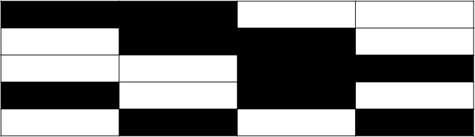
We study the finite-sample performance of the likelihood-based estimator. We consider two settings: (1) N=5000N=5000 and J=200J=200, and (2) N=10000N=10000 and J=400J=400. Missing data are generated under a block-wise design. That is, we split the rows into five equal-sized clusters and the columns into four equal-sized clusters. We let each row cluster correspond to the columns from a distinct combination of two column clusters. Rows from the same cluster have the same missing pattern. Specifically, their entries are observable and only observable on the columns that this row cluster corresponds to. This missing data pattern can be illustrated by a five-by-four block-wise matrix {(1,0,0,1,0)T,(1,1,0,0,1)T,(0,1,1,1,0)T,(0,0,1,0,1)T}\{(1,0,0,1,0)^{T},(1,1,0,0,1)^{T},(0,1,1,1,0)^{T},(0,0,1,0,1)^{T}\}, where 1 and 0 represent a submatrix with zi​j=1z_{ij}=1 and 0, respectively. An illustration of the missing pattern ZZ is illustrated in Figure 2. Under the first setting, N∗=2000,N∗=3000N_{*}=2000,N^{*}=3000, and J∗=J∗=100J_{*}=J^{*}=100. Under the second setting, N∗=4000,N∗=6000N_{*}=4000,N^{*}=6000, and J∗=J∗=200J_{*}=J^{*}=200. For each setting, θ\theta is simulated from a uniform distribution over the space {x=(x1,…,xN)T:∑i=1Nxi=0,−2≤xi≤2}\{x=(x_{1},...,x_{N})^{T}:\sum_{i=1}^{N}x_{i}=0,-2\leq x_{i}\leq 2\}, and β\beta is obtained by simulating βj\beta_{j} independently from the uniform distribution over the interval [−2,2][-2,2]. For each setting, 2000 independent datasets are generated from the considered model.

Refer to caption
Figure 2: A heat map of ZZ. The black and white regions correspond to zi​j=1z_{ij}=1 and 0, respectively.

Under setting (1), the mean squared estimation errors for MM, θ\theta, and β\beta are 0.067, 0.064, and 0.0028, respectively, across all relevant entries and all 2000 independent samples. Under setting (2), these values read 0.033, 0.031 and 0.0013, respectively. Unsurprisingly, increasing sample sizes can improve estimation accuracy.

We then examine the variance approximation in Theorem 13. We compare σ^2​(g)\hat{\sigma}^{2}(g), σ~2​(g)\tilde{\sigma}^{2}(g) and s2​(g)s^{2}(g), where s2​(g)s^{2}(g) denotes the sample variance of g⁡(M^)g(\hat{M}) that is calculated based on the 2000 simulations. As σ^2​(g)\hat{\sigma}^{2}(g) varies across the datasets, we calculate σ¯2​(g)\bar{\sigma}^{2}(g) as the average of σ^2​(g)\hat{\sigma}^{2}(g) over 2000 simulated datasets. We consider functions g⁡(M)=mi​j,θi,βjg(M)=m_{ij},\theta_{i},\beta_{j}, i=1,…,N,j=1,…,Ji=1,...,N,j=1,...,J. The results are given in Figure 3, where panels (a)-(c) show the scatter plots of s2​(g){s}^{2}(g) against σ¯2​(g)\bar{\sigma}^{2}(g) and panels (d)-(f) show those of s2​(g)s^{2}(g) against σ~2​(g)\tilde{\sigma}^{2}(g). These plots suggest that σ¯2​(g)\bar{\sigma}^{2}(g), σ~2​(g)\tilde{\sigma}^{2}(g), and s2​(g)s^{2}(g) are close to each other, for the specific forms of gg that are examined.

Figure 3: Panels (a)-(c) plot s2​(g)s^{2}(g) against σ¯2​(g)\bar{\sigma}^{2}(g) for g⁡(M)=mi​jg(M)=m_{ij}, θi\theta_{i}, and βj\beta_{j}, respectively, for fixed block-wise setting. Panels (d)-(f) plot s2​(g)s^{2}(g) against σ~2​(g)\tilde{\sigma}^{2}(g) for g⁡(M)=mi​jg(M)=m_{ij}, θi\theta_{i} and βj\beta_{j}, respectively, for fixed block-wise setting. Each panel shows 100 randomly sampled mi​jm_{ij}, θi\theta_{i}, or βj\beta_{j} under each setting. The line y=xy=x is given as a reference.

To validate asymptotic normality, we compare the empirical densities of the 2000 sample estimates of m11m_{11}, θ1\theta_{1} and β1\beta_{1} against their respective theoretical normal density curves in Figure 4 for illustration. We can observe from Figure 4 that the empirical distributions of the estimates agree well with their corresponding theoretical distributions.

Figure 4: Panels (a)-(c) presents the empirical densities (histograms) of m^11\hat{m}_{11}, θ^1\hat{\theta}_{1} and β^1\hat{\beta}_{1} under setting (1), respectively, out of 2000 simulations for fixed block-wise setting. Panels (e)-(g) presents the empirical densities of m^11\hat{m}_{11}, θ^1\hat{\theta}_{1} and β^1\hat{\beta}_{1} under setting (2), respectively, out of 2000 simulations, for fixed block-wise setting. The curves are theoretical density curves of N(m11,σ~2​(m11))(m_{11},\tilde{\sigma}^{2}(m_{11})), N(θ1,σ~2​(θ1))(\theta_{1},\tilde{\sigma}^{2}(\theta_{1})) and N(β1,σ~2​(β1)),(\beta_{1},\tilde{\sigma}^{2}(\beta_{1})), respectively, included as references.

Furthermore, for each mi​jm_{ij}, θi\theta_{i}, and βj\beta_{j}, we construct its 95% Wald interval based on (5), for which the empirical coverage based on 2000 independent replications is computed. This result is shown in Figure 5, where the two panels correspond to the two simulation settings, respectively. In each panel, the three box plots show the empirical coverage probabilities for entries of MM, θ\theta, and β\beta, respectively. As we can see, all these empirical coverage probabilities are close to the nominal level of 95%.

We also report the average number of iterations for convergence and the average CPU time per iteration as follows. For the above designs, the average number of iterations and average CPU time per iteration are (a) 184.70 and 9.24 seconds under setting 1; (b) 176.46 and 47.18 seconds under setting 2. The convergence criteria is set to be the consecutive change in the joint log-likelihood is smaller than 0.001.

Refer to caption
Figure 5: Panels (a) and (b) show the empirical coverage rates for the 95% Wald intervals under fixed block-wise settings (1) and (2), respectively.

In addition, to further demonstrate the performance of the likelihood-based estimator, we also conduct a simulation study where zi​jz_{ij} are randomly sampled under the setting that N=5000N=5000 and J=200J=200. Let zi​jz_{ij} be sampled i.i.d. from a Bernoulli distribution with P⁡(zi​j=1)=0.5P(z_{ij}=1)=0.5. The generation of the rest of the parameters and the evaluation techniques for the estimators are the same as in study under fixed block-wise setting. Under random sampling setting, the mean squared estimation errors for MM, θ\theta, and β\beta are 0.068, 0.064, and 0.0027, respectively, across all relevant entries and all 2000 independent samples. The average number of iterations and average CPU time per iteration are 182.55 and 13.93 seconds.

To examine the variance approximation under random sampling setting, we compare σ^2​(g)\hat{\sigma}^{2}(g), σ~2​(g)\tilde{\sigma}^{2}(g) and s2​(g)s^{2}(g) using the scatter plots of s2​(g){s}^{2}(g) against σ¯2​(g)\bar{\sigma}^{2}(g) in panels (a)-(c) of Figure 6 and the scatter plots of s2​(g)s^{2}(g) against σ~2​(g)\tilde{\sigma}^{2}(g) in panels (d)-(f) of Figure 6, based on the 2000 simulation replications. From Figure 6, we see that under random sampling setting, the σ¯2​(g)\bar{\sigma}^{2}(g), σ~2​(g)\tilde{\sigma}^{2}(g), and s2​(g)s^{2}(g) are close to each other for different g⁡(M)g(M).

To check the asymptotic normality under the random sampling setting, Figure 7 presents the empirical densities of the estimates densities of m11m_{11}, θ1\theta_{1} and β1\beta_{1} over 2000 samples against theoretical curves. The plots show that the empirical distributions agree well with the theoretical normal distributions. Figure 8 further shows the empirical coverage of 95%\% Wald intervals over the 2000 replications for M,θM,\theta, and β\beta. These plots suggest the empirical coverage probabilities are close to the nominal level of 95%\%.

Figure 6: Panels (a)-(c) plot s2​(g)s^{2}(g) against σ¯2​(g)\bar{\sigma}^{2}(g) for g⁡(M)=mi​jg(M)=m_{ij}, θi\theta_{i}, and βj\beta_{j}, respectively, and Panels (d)-(f) plot s2​(g)s^{2}(g) against σ~2​(g)\tilde{\sigma}^{2}(g) for g⁡(M)=mi​jg(M)=m_{ij}, θi\theta_{i} and βj\beta_{j}, respectively, for the random design setting. Each panel shows 100 randomly sampled mi​jm_{ij}, θi\theta_{i}, or βj\beta_{j} under each setting. The line y=xy=x is given as a reference.
Figure 7: Panels (a)-(c) presents the empirical densities (histograms) of m^11\hat{m}_{11}, θ^1\hat{\theta}_{1} and β^1\hat{\beta}_{1} for the random design setting, respectively. The curves are theoretical density curves of N(m11,σ~2​(m11))(m_{11},\tilde{\sigma}^{2}(m_{11})), N(θ1,σ~2​(θ1))(\theta_{1},\tilde{\sigma}^{2}(\theta_{1})) and N(β1,σ~2​(β1)),(\beta_{1},\tilde{\sigma}^{2}(\beta_{1})), respectively, included as references.
Figure 8: Boxplots of the empirical coverage rates for the 95% Wald intervals under the random design setting.

5 Real-data Applications

In what follows, we consider two real-data applications.

5.1 Application to Educational Testing

We first apply the proposed method to link two forms of an educational test that share common items. The dataset is a benchmark dataset for studying linking methods for educational testing (González and Wiberg 2017). It contains binary responses from two forms of a college admission test. Each form has 120 items and is answered by 2000 examinees. There are 40 common items shared by the two test forms. There is no missing data within each test. Thus, N=4000N=4000, J=200J=200, and 40% of the data entries are missing. We apply the proposed method to this dataset. Making use of Theorem 13, 95% confidence intervals are obtained for both the row (i.e., person) parameters and the column (i.e., item) parameters. The results allow us to compare students who took different test forms, as well as non-common items from the two forms. For illustration, we randomly choose 100 row parameters and 100 column parameters and show their 95% confidence intervals in Figure 9. Such uncertainty quantification can be vital for colleges when making admission decisions.

Figure 9: (a) 95% confidence intervals of 100 row parameters, with 50 randomly selected from each group. (b) 95% confidence intervals of the 100 column parameters, with 40 each randomly chosen from group 1 and group 2 and 20 randomly selected from anchor items (i.e., common items).

5.2 Application to Senate Voting

We now apply the proposed method to the United States senate roll call voting data. Data from the 111th through the 113th congress that include the voting records from January 11, 2009, to December 16, 2014. Quite a few senators did not serve for the entire period.

To apply our method to senators’ roll call voting records with θi\theta_{i} being interpreted as the conservativeness score of senator ii, we pre-process the data as follows. First, five senators who did not serve for more than half a year during the period are removed from the dataset, including Edward M. Kennedy, Joe Biden, Hilary Clinton, Julia Salazar, and Carte Goodwin. Second, 191 bills are removed, as all the observed votes for each of these bills are the same, and consequently, their maximum likelihood estimates do not exist. After these two steps, the resulting dataset contains N=139N=139 senators and J=1648J=1648 bills. Finally, for bill jj that has higher percentage support within the Republican party than that within the Democratic party, we let Yi​j=1Y_{ij}=1 if senator ii voted for the bill and Yi​j=0Y_{ij}=0 if senator ii voted against it. For bill jj that has higher percentage support within the Democratic party than that within the Republican party, we let Yi​j=1Y_{ij}=1 if senator ii voted against the bill and Yi​j=0Y_{ij}=0 if he/she voted for it. The value of Yi​jY_{ij} is missing if the senator chose not to vote or he/she was not in the senate when this bill was voted. For the final data being analyzed, the proportion of missing entries is 26.1%, and the connectedness Condition 2 is satisfied. The missingness pattern of the dataset is given in Figure 10. Note that in this example, N<JN<J. However, our asymptotic results are still applicable if we simply switch the roles of NN and JJ in the required conditions.

Our asymptotic results allow us to compare senators’ ideological positions, even if they did not serve in the senate at the same time. For example, Judd Gregg served in the senate between January 3, 1993, and January 3, 2011, while Marco Rubio started his first term as a senator on January 3, 2011. In our model, Judd Gregg (θi\theta_{i}) and Marco Rubio (θk\theta_{k}) have estimated conservativeness scores of 2.59 and 4.25, respectively. Applying our asymptotic results, we have θ^i−θ^k=−1.66\hat{\theta}_{i}-\hat{\theta}_{k}=-1.66 and its standard error is 0.169. If we test H0:θi=θkH_{0}:\theta_{i}=\theta_{k} against H1:θi≠θkH_{1}:\theta_{i}\neq\theta_{k}, we obtain an extremely small p-value of 9.0×10−23.9.0\times 10^{-23}. Therefore, we conclude that senator Marco Rubio is significantly more conservative than senator Judd Gregg.

In addition, we present in Tables 1 and 2 the ten senators with the largest row parameter estimates and the ten senators with the smallest row parameter estimates. These results align well with the public perceptions of these senators. For example, Jim Demint, who is ranked the most conservative senator in this dataset by our method, was also identified by Salon as one of the most conservative members of the Senate (Kornacki 2011). Our method ranks Mike Lee second, though his conservativeness score is not significantly different from that of Demint. In fact, in 2017, the New York Times used the NOMINATE system (Poole and Rosenthal 2001) to arrange Republican senators by ideology and ranked Lee as the most conservative member of the Senate (Parlapiano et al. 2017). For another example, Brian Schatz, ranked the most liberal senator by our method, is well-known as a liberal Democrat. During his time in the Senate, he voted with the Democratic party on most issues.

Finally, the 95% confidence intervals for all the row parameters are shown in Figure 11, and a full list of rankings for all 139 senators is given in the Appendices, where the corresponding row parameter estimates and their standard errors are also presented.

Refer to caption
Figure 10: A heat map of ZZ. The black and white regions correspond to zi​j=1z_{ij}=1 and 0, respectively.
Rank Senator (party) State Conservativeness Score (s.e.(θ^CLOSE(\hat{\theta}))
1 Jim DeMint (Rep) South Carolina 5.87 (0.157)
2 Mike Lee (Rep) Utah 5.73 (0.138)
3 Ted Cruz (Rep) Texas 5.65 (0.195)
4 Tom Coburn (Rep) Oklahoma 5.25 (0.114)
5 Rand Paul (Rep) Kentucky 5.24 (0.129)
6 Tim Scott (Rep) South Carolina 5.17 (0.176)
7 Jim Bunning (Rep) Kentucky 4.92 (0.204)
8 Ron Johnson (Rep) Wisconsin 4.84 (0.119)
9 James Risch (Rep) Idaho 4.81 (0.102)
10 Jim Inhofe (Rep) Oklahoma 4.69 (0.103)
Table 1: Ranking of the top 10 most conservative senators predicted by the model. Rep and Dem represent the Republican party and the Democratic party, respectively.
Rank Senator (party) State Conservativeness Score (s.e.(θ^)(\hat{\theta}))
1 Brian Schatz (Dem) Hawaii -4.74 (0.468)
2 Roland Burris (Dem) Illinois -4.43 (0.297)
3 Mazie Hirono (Dem) Hawaii -4.17 (0.383)
4 Cory Booker (Dem) New Jersey -4.14 (0.572)
5 Tammy Baldwin (Dem) Wisconsin -3.90 (0.352)
6 Sherrod Brown (Dem) Ohio -3.89 (0.168)
7 Tom Udall (Dem) New Mexico -3.85 (0.165)
8 Dick Durbin (Dem) Illinois -3.83 (0.164)
9 Ben Cardin (Dem) Maryland -3.82 (0.163)
10 Sheldon Whitehouse (Dem) Rhode Island -3.74 (0.163)
Table 2: Ranking of the top 10 most liberal senators predicted by the model. Rep and Dem represent the Republican party and the Democratic party, respectively.
Refer to caption
Figure 11: 95% confidence intervals of 139 row (i.e. senator) parameters.

6 Discussions

This note considers the statistical inference for binary (or 1-bit) matrix completion under a unidimensional nonlinear factor model, the Rasch model. Asymptotic normality results are established. Our results suggest that the maximum likelihood estimator is statistically efficient, even though the number of parameters diverges. Our simulation study shows that the developed asymptotic result provides a good approximation to finite sample data, and two real-data examples demonstrate its usefulness in the areas of educational testing and political science. One limitation of the current asymptotic normality result is that it requires relatively strong conditions, especially Condition 4(a), which excludes settings where J∗=O⁡(N∗1/2)J_{*}=O(N_{*}^{1/2}). Thus, future research is needed to investigate the extent to which these conditions can be relaxed.

The current results can be easily extended to matrix completion problems with a quantized measurement that has a similar natural exponential family form. Admittedly, the model considered may be oversimple for complex application problems, for example, certain collaborative filtering problems for which the rank of the underlying matrix MM may be higher than considered here, and the underlying latent factors may be multi-dimensional. The extension of the current results to more flexible models is left for future investigation. As the first inference result for binary matrix completion, we believe the current results will shed light on the statistical inference for more general matrix completion problems.

acknowledgments-disclosure-of-funding.
This research is partially supported by National Science Foundation CAREER SES-1846747 and Institute of Education Sciences R305D200015.

References

  • Andersen (1972) Erling B Andersen. The numerical solution of a set of conditional estimation equations. Journal of the Royal Statistical Society: Series B (Methodological), 34(1):42–54, 1972.
  • Andersen (1973) Erling B Andersen. Conditional inference and models for measuring. Mentalhygiejnisk Forlag, Copenhagen, Denmark, 1973.
  • Andersen (1970) Erling Bernhard Andersen. Asymptotic properties of conditional maximum-likelihood estimators. Journal of the Royal Statistical Society: Series B (Methodological), 32(2):283–301, 1970.
  • Beck and Teboulle (2009) Amir Beck and Marc Teboulle. Gradient-based algorithms with applications to signal recovery. Convex optimization in signal processing and communications, pages 42–88, 2009.
  • Berk (1972) Robert H Berk. Consistency and asymptotic normality of MLE’s for exponential models. The Annals of Mathematical Statistics, 43:193–204, 1972.
  • Bhaskar (2016) Sonia A Bhaskar. Probabilistic low-rank matrix completion from quantized measurements. The Journal of Machine Learning Research, 17(1):2131–2164, 2016.
  • Bhaskar and Javanmard (2015) Sonia A Bhaskar and Adel Javanmard. 1-bit matrix completion under exact low-rank constraint. In 2015 49th Annual Conference on Information Sciences and Systems (CISS), pages 1–6. IEEE, 2015.
  • Biswas et al. (2006) Pratik Biswas, T. Lian, T. Wang, and Yinyu Ye. Semidefinite programming based algorithms for sensor network localization. ACM Transactions on Sensor Networks (TOSN), 2(2):188–220, 2006.
  • Bollobás and Klee (1984) Béla Bollobás and Victor Klee. Diameters of random bipartite graphs. Combinatorica, 4(1):7–19, 1984.
  • Boyd et al. (2004) Stephen Boyd, Stephen P Boyd, and Lieven Vandenberghe. Convex optimization. Cambridge university press, 2004.
  • Bradley and Terry (1952) Ralph Allan Bradley and Milton E Terry. Rank analysis of incomplete block designs: I. the method of paired comparisons. Biometrika, 39(3/4):324–345, 1952.
  • Cai and Zhou (2013) Tony Cai and W. Zhou. A max-norm constrained minimization approach to 1-bit matrix completion. The Journal of Machine Learning Research, 14:3619–3647, 2013.
  • Candès and Recht (2009) Emmanuel J Candès and Benjamin Recht. Exact matrix completion via convex optimization. Foundations of Computational Mathematics, 9(6):717–772, 2009.
  • Candès and Tao (2010) Emmanuel J Candès and Terence Tao. The power of convex relaxation: Near-optimal matrix completion. IEEE Transactions on Information Theory, 56(5):2053–2080, 2010.
  • Chatterjee et al. (2011) Sourav Chatterjee, Persi Diaconis, Allan Sly, et al. Random graphs with a given degree sequence. Annals of Applied Probability, 21(4):1400–1435, 2011.
  • Chen and Li (2022) Yunxiao Chen and Xiaoou Li. Determining the number of factors in high-dimensional generalized latent factor models. Biometrika, 109(3):769–782, 2022.
  • Chen et al. (2019) Yuxin Chen, Jianqing Fan, Cong Ma, and Yuling Yan. Inference and uncertainty quantification for noisy matrix completion. Proceedings of the National Academy of Sciences, 116(46):22931–22937, 2019.
  • Chen et al. (2020) Yuxin Chen, Yuejie Chi, Jianqing Fan, Cong Ma, and Yuling Yan. Noisy matrix completion: Understanding statistical guarantees for convex relaxation via nonconvex optimization. SIAM Journal on Optimization, 30(4):3098–3121, 2020.
  • Davenport et al. (2014) Mark A Davenport, Yaniv Plan, Ewout Van Den Berg, and Mary Wootters. 1-bit matrix completion. Information and Inference: A Journal of the IMA, 3:189–223, 2014.
  • Embretson and Reise (2013) S.E. Embretson and S.P. Reise. Item Response Theory. Multivariate Applications Series. Taylor & Francis, 2013. URL https://books.google.com/books?id=AcWQtfGjCawC.
  • Gao et al. (2021) Chao Gao, Yandi Shen, and Anderson Y Zhang. Uncertainty quantification in the bradley-terry-luce model. arXiv preprint arXiv:2110.03874, 2021.
  • Ghosh (1995) Malay Ghosh. Inconsistent maximum likelihood estimators for the rasch model. Statistics & Probability Letters, 23(2):165–170, 1995.
  • Goldberg et al. (1992) David Goldberg, David Nichols, Brian M Oki, and Douglas Terry. Using collaborative filtering to weave an information tapestry. Communications of the ACM, 35(12):61–70, 1992.
  • González and Wiberg (2017) Jorge González and Marie Wiberg. Applying Test Equating Methods. Springer, New York, 2017.
  • Gutman et al. (2011) Roee Gutman, Gayle DeDe, David Caplan, and Jun S Liu. Rasch model and its extensions for analysis of aphasic deficits in syntactic comprehension. Journal of the American Statistical Association, 106(496):1304–1316, 2011.
  • Haberman (1977) Shelby J Haberman. Maximum likelihood estimates in exponential response models. The Annals of Statistics, 5:815–841, 1977.
  • Hagquist and Andrich (2017) Curt Hagquist and David Andrich. Recent advances in analysis of differential item functioning in health research using the Rasch model. Health and Quality of Life Outcomes, 15(1):1–8, 2017.
  • Han et al. (2020) Ruijian Han, Rougang Ye, Chunxi Tan, and Kani Chen. Asymptotic theory of sparse bradley–terry model. Annals of Applied Probability, 30:2491–2515, 2020.
  • He and Shao (2000) Xuming He and Q. Shao. On parameters of increasing dimensions. Journal of Multivariate Analysis, 73(1):120–135, 2000.
  • Kantorovich and Akilov (1964) L. Kantorovich and G.P. Akilov. Functional Analysis in Normed Spaces (translated by D.G. Brown). Pergamon Presss, Oxford, 1964.
  • Keshavan et al. (2010) Raghunandan H Keshavan, Andrea Montanari, and Sewoong Oh. Matrix completion from noisy entries. The Journal of Machine Learning Research, 11:2057–2078, 2010.
  • Kidwell et al. (2011) Paul Kidwell, Guy Lebanon, and Kevyn Collins-Thompson. Statistical estimation of word acquisition with application to readability prediction. Journal of the American Statistical Association, 106(493):21–30, 2011.
  • Klopp et al. (2015) Olga Klopp, Jean Lafond, Eric Moulines, and Joseph Salmon. Adaptive multinomial matrix completion. Electronic Journal of Statistics, 9(2):2950–2975, 2015.
  • Kolen and Brennan (2014) Michael J Kolen and Robert L Brennan. Test equating, scaling, and linking: Methods and practices. Springer Science & Business Media, 2014.
  • Koltchinskii et al. (2011) Vladimir Koltchinskii, Karim Lounici, and Alexandre B Tsybakov. Nuclear-norm penalization and optimal rates for noisy low-rank matrix completion. The Annals of Statistics, 39(5):2302–2329, 2011.
  • Kornacki (2011) Steve Kornacki. Why healthcare may not doom mitt romney after all. https://www.salon.com/2011/05/12/romney_healthcare/, 2011.
  • Lindsay et al. (1991) Bruce Lindsay, Clifford C Clogg, and John Grego. Semiparametric estimation in the Rasch model and related exponential response models, including a simple latent class model for item analysis. Journal of the American Statistical Association, 86(413):96–107, 1991.
  • Liu and Vandenberghe (2010) Zhang Liu and Lieven Vandenberghe. Interior-point method for nuclear norm approximation with application to system identification. SIAM Journal on Matrix Analysis and Applications, 31(3):1235–1256, 2010.
  • Negahban and Wainwright (2012) Sahand Negahban and Martin J Wainwright. Restricted strong convexity and weighted matrix completion: optimal bounds with noise. The Journal of Machine Learning Research, 13(1):1665–1697, 2012.
  • Neyman and Scott (1948) Jerzy Neyman and Elizabeth L Scott. Consistent estimates based on partially consistent observations. Econometrica, 16:1–32, 1948.
  • Parlapiano et al. (2017) A. Parlapiano, W. Andrews, and R. Lee, J.and Shorey. How each senator voted on obamacare repeal proposals. https://www.nytimes.com/interactive/2017/07/25/us/politics/senate-votes-repeal-obamacare.html, 2017.
  • Poole and Rosenthal (1991) Keith T Poole and Howard Rosenthal. Patterns of congressional voting. American Journal of Political Science, 35:228–278, 1991.
  • Poole and Rosenthal (2001) Keith T Poole and Howard Rosenthal. Dnominate after 10 years: A comparative update to congress: a political-economic history of roll-call voting. Legislative Studies Quarterly, 26:5–29, 2001.
  • Poole et al. (1991) Keith T Poole, Howard Rosenthal, and Kenneth Koford. On dimensionalizing roll call votes in the us congress. The American Political Science Review, 85:955–976, 1991.
  • Portnoy (1988) Stephen Portnoy. Asymptotic behavior of likelihood methods for exponential families when the number of parameters tends to infinity. The Annals of Statistics, 16:356–366, 1988.
  • Rao (1973) C. Radhakrishna Rao. Linear statistical inference and its applications. Wiley New York, 1973.
  • Rasch (1960) Georg Rasch. Studies in mathematical psychology: I. Probabilistic models for some intelligence and attainment tests. Nielsen & Lydiche, Oxford, England, 1960.
  • Rice (2004) Kenneth M Rice. Equivalence between conditional and mixture approaches to the Rasch model and matched case-control studies, with applications. Journal of the American Statistical Association, 99(466):510–522, 2004.
  • Rinaldo et al. (2013) Alessandro Rinaldo, Sonja Petrović, and Stephen E Fienberg. Maximum lilkelihood estimation in the β\beta-model. The Annals of Statistics, 41:1085–1110, 2013.
  • Simons and Yao (1999) Gordon Simons and Y. Yao. Asymptotics when the number of parameters tends to infinity in the bradley-terry model for paired comparisons. The Annals of Statistics, 27:1041–1060, 1999.
  • van der Linden and Hambleton (2013) Wim J van der Linden and Ronald K Hambleton. Handbook of modern item response theory. Springer, New York, NY, 2013.
  • Van Handel (2014) Ramon Van Handel. Probability in high dimension. Technical report, PRINCETON UNIV NJ, 2014.
  • Wang (2011) Lan Wang. GEE analysis of clustered binary data with diverging number of covariates. The Annals of Statistics, 39(1):389–417, 2011.
  • Xia and Yuan (2021) Dong Xia and Ming Yuan. Statistical inferences of linear forms for noisy matrix completion. Journal of the Royal Statistical Society: Series B (Statistical Methodology), 83(1):58–77, 2021.
  • Yan et al. (2011) Ting Yan, Yuanzhang Li, Jinfeng Xu, Yaning Yang, and Ji Zhu. Wilks’ theorems in some exponential random graph models. arXiv preprint arXiv:1201.0058, 2011.

Appendix

The appendix contains the proofs of theorems and proposition in Appendix A, the proofs of the supporting lemmas in Appendix B, and additional real-data application results from Section 5.2 “Application to Senate Voting” in Appendix C.

Appendix A: Proof of Theorems and Proposition

Appendix A contains proofs of the theorems and the proposition developed in the main article.

Proof of Theorem 9.

This result is directly implied by Theorem B of Bollobás and Klee 1984, which shows that under the conditions of Theorem 9, with probability tending to 1, the corresponding bipartite random graph has diameter no larger than n+1n+1. This result combined with the fact that a graph is connected if and only if its diameter is finite proves Theorem 9. ∎

We now focus on the rest of the theorems and propositions. We start with defining some notation. Implicitly index JJ with NN such that JN→∞J_{N}\to\infty as N→∞N\to\infty for notation convenience. Note that this does not impose any rate requirement for NN and J.J. Let ΩN={x=(xi​j:zi​j=1,i=1,…,N,j=1,…,J):xi​j=θi−βj,θi,βj∈ℝ,∑i=1Nθi=0}\Omega_{N}=\big\{x=(x_{ij}:z_{ij}=1,i=1,...,N,j=1,...,J):x_{ij}=\theta_{i}-\beta_{j},\theta_{i},\beta_{j}\in\mathbb{R},\sum_{i=1}^{N}\theta_{i}=0\big\} be a vector space. Define on ΩN\Omega_{N} a variance weighted inner product [⋅,⋅]σ[\cdot,\cdot]_{\sigma} with [x,y]σ=∑i=1N∑j∈SJ​(i)xi​j​σi​j2​yi​j[x,y]_{\sigma}=\sum_{i=1}^{N}\sum_{j\in S_{J}(i)}x_{ij}\sigma_{ij}^{2}y_{ij} for any x,y∈ΩN,x,y\in\Omega_{N}, where SJ(i)={j=1,…,J:zi​j=1}S_{J}(i)=\{j=1,...,J:z_{ij}=1\}, σi​j2=exp⁡(mi​j∗)/{1+exp⁡(mi​j∗)}2\sigma_{ij}^{2}=\exp(m_{ij}^{*})/\{1+\exp(m_{ij}^{*})\}^{2} and the subscript σ\sigma means the inner product depends on σi​j2,i=1,…,N,j=1,…,J,zi​j=1\sigma_{ij}^{2},i=1,...,N,j=1,...,J,z_{ij}=1. Denote the associated norm as ∥⋅∥σ\|\cdot\|_{\sigma} with ‖x‖σ2=∑i=1N∑j∈SJ​(i)xi​j2​σi​j2\|x\|_{\sigma}^{2}=\sum_{i=1}^{N}\sum_{j\in S_{J}(i)}x_{ij}^{2}\sigma_{ij}^{2} for x∈ΩN.x\in\Omega_{N}. Let MN=(mi​j:zi​j=1,i=1,…,N,j=1,…,J,mi​j=θi−βj)∈ΩNM_{N}=\big(m_{ij}:z_{ij}=1,i=1,...,N,j=1,...,J,m_{ij}=\theta_{i}-\beta_{j})\in\Omega_{N}, MN∗=(mi​j∗:zi​j=1,i=1,…,N,j=1,…,J,mi​j∗=θi∗−βj∗)∈ΩNM_{N}^{*}=\big(m_{ij}^{*}:z_{ij}=1,i=1,...,N,j=1,...,J,m_{ij}^{*}=\theta_{i}^{*}-\beta_{j}^{*})\in\Omega_{N} and M^N=(m^i​j:zi​j=1,i=1,…,N,j=1,…,J,m^i​j=θ^i−β^j)∈ΩN.\hat{M}_{N}=\big(\hat{m}_{ij}:z_{ij}=1,i=1,...,N,j=1,...,J,\hat{m}_{ij}=\hat{\theta}_{i}-\hat{\beta}_{j})\in\Omega_{N}. Note that as a result of Proposition 7, for any linear form gg of MM, g⁡(M)g(M) can be re-expressed as a linear form of x∈ΩNx\in\Omega_{N}, with g⁡(x)=∑i=1N∑j∈SJ​(i)wi​j​xi​jg(x)=\sum_{i=1}^{N}\sum_{j\in S_{J}(i)}w_{ij}x_{ij}, where we denote wi​j=wi​j​(g)w_{ij}=w_{ij}(g), which depends on gg, for notation simplicity. Let ΩN∗\Omega_{N}^{*} consist of all linear forms gg on ΩN\Omega_{N} such that g⁡(x)=0g(x)=0 if x=0x=0 and x∈ΩN.x\in\Omega_{N}. Without loss of generality, we will work with g∈ΩN∗g\in\Omega_{N}^{*} in the proofs. For any subset A⊂ΩN∗A\subset\Omega_{N}^{*}, define ∥⋅∥σ(A)\|\cdot\|_{\sigma}(A) to be the norm on ΩN\Omega_{N} such that for any x∈ΩNx\in\Omega_{N}, ‖x‖σ​(A)\|x\|_{\sigma}(A) is the smallest non-negative number such that |g⁡(x)|≤‖x‖σ​(A)​σ​(g)|g(x)|\leq\|x\|_{\sigma}(A)\sigma(g) for any g∈A,g\in A, where σ⁡(g)=supx∈ΩN{|g⁡(x)|:‖x‖σ≤1}.\sigma(g)=\sup_{x\in\Omega_{N}}\{|g(x)|:\|x\|_{\sigma}\leq 1\}. Let

EN=(Ei​j:zi​j=1,i=1,…,N,j=1,…,J),E_{N}=\Big(E_{ij}:z_{ij}=1,i=1,...,N,j=1,...,J\Big),

with Ei​j=𝔼⁡[Yi​j]=emi​j∗/(1+emi​j∗),E_{ij}=\mathbb{E}[Y_{ij}]=e^{m_{ij}^{*}}/(1+e^{m_{ij}^{*}}), be the vector of expected responses corresponding to the observed entries. Further define RN∈ΩNR_{N}\in\Omega_{N} satisfying

[x,RN]σ=∑i=1N∑j∈SJ​(i)xi​j​(Yi​j−Ei​j),x∈ΩN.[x,R_{N}]_{\sigma}=\sum_{i=1}^{N}\sum_{j\in S_{J}(i)}x_{ij}(Y_{ij}-E_{ij}),\quad\quad x\in\Omega_{N}.

Define an evaluation measure UN​(⋅,⋅)U_{N}(\cdot,\cdot) such that for any y,v∈ΩNy,v\in\Omega_{N}, UN​(y,v)∈ΩNU_{N}(y,v)\in\Omega_{N} satisfies

[x,UN​(y,v)]σ=∑i=1N∑j∈SJ​(i)xi​j​{σ2​(yi​j)−σi​j2}​vi​j,x∈ΩN,[x,U_{N}(y,v)]_{\sigma}=\sum_{i=1}^{N}\sum_{j\in S_{J}(i)}x_{ij}\big\{\sigma^{2}(y_{ij})-\sigma_{ij}^{2}\big\}v_{ij},\quad\quad x\in\Omega_{N},

where σ2​(yi​j)=eyi​j/(1+eyi​j)2\sigma^{2}(y_{ij})=e^{y_{ij}}/(1+e^{y_{ij}})^{2}. Note when yy is equal to MN∗M_{N}^{*} or when vv is a zero vector, then UN​(y,v)=0.U_{N}(y,v)=0. Further denote that wi+=∑j∈SJ​(i)wi​j,w_{i+}=\sum_{j\in S_{J}(i)}w_{ij}, w+j=∑i∈SN​(j)wi​jw_{+j}=\sum_{i\in S_{N}(j)}w_{ij} and w+⁣+=∑i=1N∑j∈SJ​(i)wi​jw_{++}=\sum_{i=1}^{N}\sum_{j\in S_{J}(i)}w_{ij}, where SN(j)={i=1,…,N:zi​j=1}S_{N}(j)=\{i=1,...,N:z_{ij}=1\}. We first give proof for Theorem 10 below.

Proof of Theorem 10.

We start with establishing the existence of M^N\hat{M}_{N} by applying the fixed point theorems of Kantorovich and Akilov 1964. We start with constructing a function FNF_{N} on ΩN\Omega_{N} with a fixed point M^N\hat{M}_{N}. Consider FN​(y)=y+rN​(y)F_{N}(y)=y+r_{N}(y) for y∈ΩNy\in\Omega_{N}, where rN:ΩN↦ΩNr_{N}:\Omega_{N}\mapsto\Omega_{N} is defined by the equation,

[x,rN​(y)]σ=∑i=1N∑j∈SJ​(i)xi​j​{Yi​j−E⁡(yi​j)},x∈ΩN,[x,r_{N}(y)]_{\sigma}=\sum_{i=1}^{N}\sum_{j\in S_{J}(i)}x_{ij}\big\{Y_{ij}-E(y_{ij})\big\},\quad\quad x\in\Omega_{N},

where E⁡(yi​j)=eyi​j/(1+eyi​j).E(y_{ij})=e^{y_{ij}}/(1+e^{y_{ij}}). Note that FNF_{N} has a fixed point ω∈ΩN\omega\in\Omega_{N} if and only if

∑i=1N∑j∈SJ​(i)xi​j​{Yi​j−E⁡(ωi​j)}=0,x∈ΩN.\sum_{i=1}^{N}\sum_{j\in S_{J}(i)}x_{ij}\big\{Y_{ij}-E(\omega_{ij})\big\}=0,\quad\quad x\in\Omega_{N}.

Let PP be the orthogonal projection onto ΩN\Omega_{N}. Let E^={E(m^i​j):i=1,…,N,j=1,…,J,zi​j=1}\hat{E}=\{E(\hat{m}_{ij}):i=1,...,N,j=1,...,J,z_{ij}=1\} and Yz={Yi​j:i=1,…,N,j=1,…,J,zi​j=1}.Y_{z}=\{Y_{ij}:i=1,...,N,j=1,...,J,z_{ij}=1\}. Then following from Berk 1972, M^N\hat{M}_{N} is a maximum likelihood estimator of MN∗M_{N}^{*} if and only if P​E^=P​Yz.P\hat{E}=PY_{z}. Hence, M^N\hat{M}_{N} exists if and only if ω\omega exists. Furthermore, since the log-likelihood l⁡(Yz,⋅)l(Y_{z},\cdot) is strictly concave, if the maximum likelihood estimator M^N\hat{M}_{N} of MN∗M_{N}^{*} exists, then it must be unique. Therefore, if M^N\hat{M}_{N} exists, ω=M^N.\omega=\hat{M}_{N}. So, we just need to verify the conditions of the fixed point theorem to show that the fixed point ω\omega indeed exists.

The Kantorovich & Akilov’s fixed point theorem requires construction of a sequence that converges to the fixed point. Consider the sequence {tN​k:k=0,1,…}\{t_{Nk}:k=0,1,...\}, with tN​0=MN∗t_{N0}=M_{N}^{*} and tN⁡(k+1)=FN​(tN​k)t_{N(k+1)}=F_{N}(t_{Nk}) for k=0,1,…k=0,1,... Note that tN​1=MN∗+RNt_{N1}=M_{N}^{*}+R_{N}. To check whether this sequence is well-defined and converges to M^N\hat{M}_{N}, we need to examine the differential d​FN​ydF_{Ny} of FNF_{N} at y∈ΩNy\in\Omega_{N}. Note that for y+v∈ΩNy+v\in\Omega_{N},

[x,FN​(y+v)−FN​(y)]σ\displaystyle[x,F_{N}(y+v)-F_{N}(y)]_{\sigma} =∑i=1N∑j∈SJ​(i)xi​j​σi​j2​[vi​j+(σi​j2)−1​{E⁡(yi​j)−E⁡(yi​j+vi​j)}]\displaystyle=\sum_{i=1}^{N}\sum_{j\in S_{J}(i)}x_{ij}\sigma_{ij}^{2}\Big[v_{ij}+(\sigma_{ij}^{2})^{-1}\big\{E(y_{ij})-E(y_{ij}+v_{ij})\big\}\Big]
=−[x,UN​(y,v)]σ+o⁡(v),\displaystyle=-[x,U_{N}(y,v)]_{\sigma}+o(v),

where o⁡(v)/‖v‖σ→0o(v)/\|v\|_{\sigma}\to 0 as ‖v‖σ→0\|v\|_{\sigma}\to 0. It follows that d​FN​y​(v)=−UN​(y,v)dF_{Ny}(v)=-U_{N}(y,v). Denote ‖d​FN​y‖σ​(A)\|dF_{Ny}\|_{\sigma}(A) to be the smallest nonnegative number such that

‖d​FN​y​(v)‖σ​(A)≤‖d​FN​y‖σ​(A)​‖v‖σ​(A),v∈ΩN.\|dF_{Ny}(v)\|_{\sigma}(A)\leq\|dF_{Ny}\|_{\sigma}(A)\|v\|_{\sigma}(A),\quad\quad v\in\Omega_{N}.

Let ApA_{p} be the set consisting of all the point maps fi​jf_{ij} on ΩN\Omega_{N}, i.e. fi​j​(x)=xi​jf_{ij}(x)=x_{ij} for any x∈ΩNx\in\Omega_{N}. By Lemma 15(c) below, there exist sequences fNf_{N} and dNd_{N} such that

‖d​FN​y‖σ​(Ap)≤dN​‖y−MN∗‖σ​(Ap)whenever‖y−MN∗‖σ​(Ap)≤fN,y∈ΩN.\|dF_{Ny}\|_{\sigma}(A_{p})\leq d_{N}\|y-M_{N}^{*}\|_{\sigma}(A_{p})\quad\text{whenever}\quad\|y-M_{N}^{*}\|_{\sigma}(A_{p})\leq f_{N},\quad y\in\Omega_{N}.
Lemma 0.

Assume Conditions 1–3 hold. If Ap={fi​j:i=1,…,N,j=1,…,J,zi​j=1}A_{p}=\{f_{ij}:i=1,...,N,j=1,...,J,z_{ij}=1\} such that fi​j​(x)=xi​jf_{ij}(x)=x_{ij} for x∈ΩNx\in\Omega_{N}. Let CN=|Ap|C_{N}=|A_{p}|, the cardinality of ApA_{p}. Then there exist sequences fN>0f_{N}>0 and dN≥0d_{N}\geq 0 satisfying the followings.

(a). As N→∞N\to\infty, fN2/log⁡CN→∞.f_{N}^{2}/\log C_{N}\to\infty.

(b). As N→∞N\to\infty, fN2​(N∗−1+J∗−1)→0.f_{N}^{2}(N_{*}^{-1}+J_{*}^{-1})\to 0.

(c). If y,v∈ΩNy,v\in\Omega_{N} and ‖y−MN∗‖σ​(Ap)≤fN\|y-M_{N}^{*}\|_{\sigma}(A_{p})\leq f_{N}, then there exists n<∞n<\infty such that for all N>nN>n, ‖UN​(y,v)‖σ​(Ap)≤dN​‖y−MN∗‖σ​(Ap)​‖v‖σ​(Ap).\|U_{N}(y,v)\|_{\sigma}(A_{p})\leq d_{N}\|y-M_{N}^{*}\|_{\sigma}(A_{p})\|v\|_{\sigma}(A_{p}). Furthermore, dN​fN→0d_{N}f_{N}\to 0 as N→∞N\to\infty.

As shown in Kantorovich and Akilov 1964, if ‖RN‖σ​(Ap)<12​fN\|R_{N}\|_{\sigma}(A_{p})<\frac{1}{2}f_{N} and dN​‖RN‖σ​(Ap)<12d_{N}\|R_{N}\|_{\sigma}(A_{p})<\frac{1}{2}, then M^N\hat{M}_{N} exists. By Lemma 16 below, we have pr(‖RN‖σ​(Ap)<12​fN)→1(\|R_{N}\|_{\sigma}(A_{p})<\frac{1}{2}f_{N})\to 1 as N→∞N\to\infty. Therefore, it follows from Lemma 15(c) that with probability tending to 1, dN​‖RN‖σ​(Ap)<12​fN​dN→0d_{N}\|R_{N}\|_{\sigma}(A_{p})<\frac{1}{2}f_{N}d_{N}\to 0.

Lemma 0.

Let A⊂ΩN∗.A\subset\Omega_{N}^{*}. Let CNC_{N} denote the cardinality of AA. If there exist sequences fN>0f_{N}>0 and dN≥0d_{N}\geq 0 satisfying (a). 0<CN<∞0<C_{N}<\infty and fN2/log⁡Cn→∞f_{N}^{2}/\log C_{n}\to\infty as N→∞,N\to\infty, (b). If y,v∈ΩNy,v\in\Omega_{N} and ‖y−MN∗‖σ​(A)≤fN\|y-M_{N}^{*}\|_{\sigma}(A)\leq f_{N}, then there exists n<∞n<\infty such that for all N>nN>n, ‖UN​(y,v)‖σ​(A)≤dN​‖y−MN∗‖σ​(A)​‖v‖σ​(A),\|U_{N}(y,v)\|_{\sigma}(A)\leq d_{N}\|y-M_{N}^{*}\|_{\sigma}(A)\|v\|_{\sigma}(A), (c). dN​fN→0d_{N}f_{N}\to 0 as N→∞N\to\infty. Then pr(‖RN‖σ​(A)<12​fN)→1\big(\|R_{N}\|_{\sigma}(A)<\frac{1}{2}f_{N}\big)\to 1 as N→∞.N\to\infty.

Hence, the conditions of the fixed point theorem are satisfied with probability approaching 1. It then follows that the maximum likelihood estimators M^N\hat{M}_{N} exists with probability tending to 1. Since Condition 2 holds, as a direct consequence of Proposition 7, the corresponding maximum likelihood estimators θ^i\hat{\theta}_{i}, i=1,…,Ni=1,...,N and β^j\hat{\beta}_{j}, j=1,…,Jj=1,...,J can be uniquely determined given M^N\hat{M}_{N}. Therefore, with probability approaching 1 that they all exist, as N→∞N\to\infty. The first part of the theorem then follows.

Now we seek to prove the consistency results. Taking sequences fNf_{N} and dNd_{N} again as satisfying the results in Lemma 15 and A=Ap.A=A_{p}. Then both Lemmas 16 and 17 hold. From the results of Lemmas 16 and 17, it can be implied that as N→∞N\to\infty, with probability tending to 1 that,

‖M^N−MN∗‖σ​(Ap)=O⁡(fN).\displaystyle\|\hat{M}_{N}-M_{N}^{*}\|_{\sigma}(A_{p})=O(f_{N}). (6)

From Haberman 1977, σ⁡(g)\sigma(g) is in fact the standard deviation of g⁡(M^N)g(\hat{M}_{N}). We further note by Lemma 18 below,

maxg∈Ap⁡σ⁡(g)≤τ2−1​(N∗−1+J∗−1)12,\displaystyle\max_{g\in A_{p}}\sigma(g)\leq\tau_{2}^{-1}(N_{*}^{-1}+J_{*}^{-1})^{\frac{1}{2}}, (7)

for some 0<τ2<∞0<\tau_{2}<\infty.

Lemma 0.

Assume Conditions 1–3 hold. Let A⊂ΩN∗.A\subset\Omega_{N}^{*}. If there exist sequences fN>0f_{N}>0 and dN≥0d_{N}\geq 0 satisfying (a). pr(‖RN‖σ​(A)<12​fN)→1\big(\|R_{N}\|_{\sigma}(A)<\frac{1}{2}f_{N}\big)\to 1 as N→∞,N\to\infty, (b). If y,v∈ΩNy,v\in\Omega_{N} and ‖y−MN∗‖σ​(A)≤fN\|y-M_{N}^{*}\|_{\sigma}(A)\leq f_{N}, then there exists n<∞n<\infty such that for all N>nN>n, ‖UN​(y,v)‖σ​(A)≤dN​‖y−MN∗‖σ​(A)​‖v‖σ​(A),\|U_{N}(y,v)\|_{\sigma}(A)\leq d_{N}\|y-M_{N}^{*}\|_{\sigma}(A)\|v\|_{\sigma}(A), (c). dN​fN→0d_{N}f_{N}\to 0 as N→∞N\to\infty. Then, as N→∞N\to\infty, with probability approaching 1 that,

|‖M^N−MN∗‖σ​(A)‖RN‖σ​(A)−1|≤dN12→0and‖M^N−MN∗−RN‖σ​(A)≤dN​‖RN‖σ2​(A).\displaystyle\Big|\frac{\|\hat{M}_{N}-M_{N}^{*}\|_{\sigma}(A)}{\|R_{N}\|_{\sigma}(A)}-1\Big|\leq d_{N}^{\frac{1}{2}}\to 0\quad\text{and}\quad\|\hat{M}_{N}-M_{N}^{*}-R_{N}\|_{\sigma}(A)\leq d_{N}\|R_{N}\|_{\sigma}^{2}(A).
Lemma 0.

Assume Conditions 1–3 hold and ∑i=1Nθi=0\sum_{i=1}^{N}\theta_{i}=0, the asymptotic variance of the maximum likelihood estimator of mi​j∗,m_{ij}^{*}, v​a​r​(m^i​j)var(\hat{m}_{ij}), for any i=1,…,Ni=1,...,N and j=1,…,Jj=1,...,J, takes the form,

v​a​r​(m^i​j)=(σi+2)−1+(σ+j2)−1+O⁡(N∗−1​J∗−1)asN→∞.\displaystyle var(\hat{m}_{ij})=(\sigma_{i+}^{2})^{-1}+(\sigma_{+j}^{2})^{-1}+O(N_{*}^{-1}J_{*}^{-1})\quad\text{as}\quad N\to\infty.

Then as N→∞N\to\infty, we have with probability approaching 1 that

maxi,j,zi​j=1⁡|m^i​j−mi​j∗|\displaystyle\max_{i,j,z_{ij=1}}|\hat{m}_{ij}-m_{ij}^{*}| =maxi,j,zi​j=1⁡|fi​j​(M^N)−fi​j​(MN∗)|\displaystyle=\max_{i,j,z_{ij=1}}|f_{ij}(\hat{M}_{N})-f_{ij}(M_{N}^{*})|
=maxi,j,zi​j=1⁡|fi​j​(M^N−MN∗)|\displaystyle=\max_{i,j,z_{ij=1}}|f_{ij}(\hat{M}_{N}-M_{N}^{*})|
≤maxi,j,zi​j=1⁡σ⁡(fi​j)​‖M^N−MN∗‖σ​(Ap)\displaystyle\leq\max_{i,j,z_{ij=1}}\sigma(f_{ij})\|\hat{M}_{N}-M_{N}^{*}\|_{\sigma}(A_{p})
≤‖M^N−MN∗‖σ​(Ap)​{maxg∈Ap⁡σ⁡(g)}\displaystyle\leq\|\hat{M}_{N}-M_{N}^{*}\|_{\sigma}(A_{p})\Big\{\max_{g\in A_{p}}\sigma(g)\Big\}
=O⁡{fN​(N∗−1+J∗−1)12}\displaystyle=O\Big\{f_{N}\left(N_{*}^{-1}+J_{*}^{-1}\right)^{\frac{1}{2}}\Big\}
→0.\displaystyle\to 0. (8)

The second last line follows from (6) and (7) and the last line follows from Lemma 15(b).

By Proposition 1, given m^i​j\hat{m}_{ij} for i=1,…,N,j=1,…,J,zi​j=1i=1,...,N,j=1,...,J,z_{ij}=1, all the θ^i\hat{\theta}_{i}, i=1,…,Ni=1,...,N and β^j\hat{\beta}_{j}, j=1,…,Jj=1,...,J can be uniquely determined. Since (8) holds, as a direct consequence of the Slutsky Theorem, we have with probability tending to 1 that ‖θ^−θ∗‖∞→0\|\hat{\theta}-\theta^{*}\|_{\infty}\to 0 and ‖β^−β∗‖∞→0\|\hat{\beta}-\beta^{*}\|_{\infty}\to 0 as N→∞N\to\infty. From here, we have maxi,j⁡|m^i​j−mi​j∗|→0\max_{i,j}|\hat{m}_{ij}-m_{ij}^{*}|\rightarrow 0. Hence we complete the proof of consistency results in this theorem.

∎

The proof of Theorem 11 is a continuum of the proof of Theorem 10 with additional conditions. We next present the proof of Theorem 11.

Proof of Theorem 11.

To derive explicit rates of convergence for ‖θ^−θ∗‖∞\|\hat{\theta}-\theta^{*}\|_{\infty} and ‖β^−β∗‖∞\|\hat{\beta}-\beta^{*}\|_{\infty}, we adopt a similar approach as in the derivation of convergence of maxi,j:zi​j=1|m^i​j−mi​j∗|.\max_{i,j:z_{ij}=1}|\hat{m}_{ij}-m_{ij}^{*}|. In particular, for the column parameters βj\beta_{j}, we consider linear functions gj∈ΩN∗g_{j}\in\Omega_{N}^{*} such that gj​(x)=βj.g_{j}(x)=\beta_{j}. We can construct gjg_{j} as follows. The idea is to include all the row parameters θi\theta_{i} so as to use the identifiability constraint ∑i=1Nθi=0\sum_{i=1}^{N}\theta_{i}=0. For any i∈SN​(j),i\in S_{N}(j), we use mi​j=θi−βjm_{ij}=\theta_{i}-\beta_{j} in the construction. While for each i∈SNϕ​(j),i\in S_{N_{\phi}}(j), where SNϕ​(j)={1,2,…,N}∖SN​(j),S_{N_{\phi}}(j)=\{1,2,...,N\}\setminus S_{N}(j), by Condition 2, there must exist 1≤ii​1,ii​2,…,ii​k≤N1\leq i_{i1},i_{i2},...,i_{ik}\leq N and 1≤ji​1,ji​2,…,ji​k≤J1\leq j_{i1},j_{i2},...,j_{ik}\leq J such that

zi,ji​1=zii​1,ji​1=zii​1,ji​2=zii​2,ji​2=…=zii​k,ji​k=zii​k,j=1.\displaystyle z_{i,j_{i1}}=z_{i_{i1},j_{i1}}=z_{i_{i1},j_{i2}}=z_{i_{i2},j_{i2}}=...=z_{i_{ik},j_{ik}}=z_{i_{ik},j}=1.

Therefore, we can construct gjg_{j} as

gj​(x)=\displaystyle g_{j}(x)= −1N{∑i∈SN​(j)mi​j\displaystyle-\frac{1}{N}\Big\{\sum_{i\in S_{N}(j)}m_{ij}
+∑i∈SNϕ​(j)(mi,ji​1−mii​1,ji​1+mii​1,ji​2−mii​2,ji​2+…−mii​k,ji​k+mii​k,j)}\displaystyle+\sum_{i\in S_{N_{\phi}}(j)}\Big(m_{i,j_{i1}}-m_{i_{i1},j_{i1}}+m_{i_{i1},j_{i2}}-m_{i_{i2},j_{i2}}+...-m_{i_{ik},j_{ik}}+m_{i_{ik},j}\Big)\Big\}
=\displaystyle= βj.\displaystyle\beta_{j}.

Let Aβ={gj:j=1,…,J}.A_{\beta}=\big\{g_{j}:j=1,...,J\big\}. Now consider a sequence fNf_{N} satisfying the rate requirements fN2/log⁡J→∞f_{N}^{2}/\log J\to\infty and fN2N∗−1/2→0f_{N}^{2}N_{*}^{-1/2}\to 0 as N→∞N\to\infty. Then by Lemma 19 below, we can pick a sequence dNd_{N} satisfying Lemma 19(a) and Lemma 19(b). Furthermore, by Lemma 20 below, we know that σ2​(gj)=(σ+j2)−1+O⁡(N∗−1​J∗−1)\sigma^{2}(g_{j})=(\sigma_{+j}^{2})^{-1}+O(N_{*}^{-1}J_{*}^{-1}) for any gj∈Aβg_{j}\in A_{\beta}. Therefore, there exist positive 0<c2<∞0<c_{2}<\infty and some nn such that for all N>n,N>n,

maxj=1,…,J⁡σ⁡(gj)<c2−1​N∗−12.\displaystyle\max_{j=1,...,J}\sigma(g_{j})<c_{2}^{-1}N_{*}^{-\frac{1}{2}}.
Lemma 0.

Assume Conditions 1–4 hold. If Aβ={gj:j=1,…,J}A_{\beta}=\{g_{j}:j=1,...,J\} such that gj∈ΩN∗g_{j}\in\Omega_{N}^{*} and gj​(x)=βjg_{j}(x)=\beta_{j} for x∈ΩNx\in\Omega_{N}. Let CN=|Aβ|=JC_{N}=|A_{\beta}|=J be the cardinality of AβA_{\beta}. For any positive sequence fNf_{N} such that fN2/log⁡J→∞f_{N}^{2}/\log J\to\infty and fN2N∗−1/2→0f_{N}^{2}N_{*}^{-1/2}\to 0 as N→∞N\to\infty, there exists a sequence dN≥0d_{N}\geq 0 satisfying the followings.

(a). If y,v∈ΩNy,v\in\Omega_{N} and ‖y−MN∗‖σ​(Aβ)≤fN\|y-M_{N}^{*}\|_{\sigma}(A_{\beta})\leq f_{N}, then there exists n<∞n<\infty such that for all N>nN>n, ‖UN​(y,v)‖σ​(Aβ)≤dN​‖y−MN∗‖σ​(Aβ)​‖v‖σ​(Aβ).\|U_{N}(y,v)\|_{\sigma}(A_{\beta})\leq d_{N}\|y-M_{N}^{*}\|_{\sigma}(A_{\beta})\|v\|_{\sigma}(A_{\beta}).

(b). dN​fN2→0d_{N}f_{N}^{2}\to 0 as N→∞N\to\infty.

Lemma 0.

Assume Conditions 1–4 hold and ∑i=1Nθi=0\sum_{i=1}^{N}\theta_{i}=0. The asymptotic variance of the maximum likelihood estimator of an individual column parameter, var(β^j)(\hat{\beta}_{j}), asymptotically attains the oracle variance (σ+j2)−1(\sigma_{+j}^{2})^{-1} in the sense that

v​a​r​(β^j)=(σ+j2)−1+O⁡(N∗−1​J∗−1)asN→∞.\displaystyle var(\hat{\beta}_{j})=(\sigma_{+j}^{2})^{-1}+O(N_{*}^{-1}J_{*}^{-1})\quad\quad\text{as}\quad N\to\infty.

Note that by taking sequences fNf_{N} and dNd_{N} satisfying the conditions in Lemma 19 and setting A=Aβ,A=A_{\beta}, it can be shown easily that the results of Lemmas 16 and 17 still hold. Hence, it can be implied that as N→∞,N\to\infty, with probability tending to 1,

‖M^N−MN∗‖σ​(Aβ)=O⁡(fN).\displaystyle\|\hat{M}_{N}-M_{N}^{*}\|_{\sigma}(A_{\beta})=O(f_{N}).

Then as N→∞N\to\infty, we have with probability approaching 1 that,

maxj=1,…,J⁡|β^j−βj∗|\displaystyle\max_{j=1,...,J}|\hat{\beta}_{j}-\beta_{j}^{*}| =maxj=1,…,J⁡|gj​(M^N)−gj​(MN∗)|\displaystyle=\max_{j=1,...,J}|g_{j}(\hat{M}_{N})-g_{j}(M_{N}^{*})|
=maxj=1,…,J⁡|gj​(M^N−MN∗)|\displaystyle=\max_{j=1,...,J}|g_{j}(\hat{M}_{N}-M_{N}^{*})|
≤‖M^N−MN∗‖σ​(Aβ)​maxj=1,…,J⁡σ⁡(gj)\displaystyle\leq\|\hat{M}_{N}-M_{N}^{*}\|_{\sigma}(A_{\beta})\max_{j=1,...,J}\sigma(g_{j})
<c2−1​N∗−12​‖M^N−MN∗‖σ​(Aβ)\displaystyle<c_{2}^{-1}N_{*}^{-\frac{1}{2}}\|\hat{M}_{N}-M_{N}^{*}\|_{\sigma}(A_{\beta})
=O{(logJ)12N∗−12}asN→∞,\displaystyle=O\Big\{(\log J)^{\frac{1}{2}}N_{*}^{-\frac{1}{2}}\Big\}\quad\text{as}\quad N\to\infty,

where the last step can be implied from the fact that ‖M^N−MN∗‖σ​(Aβ)=O⁡(fN)\|\hat{M}_{N}-M_{N}^{*}\|_{\sigma}(A_{\beta})=O\big(f_{N}\big) and the rate requirement of fNf_{N} in Lemma 19, where the minimum order of fNf_{N} is determined by fN2/log⁡J→∞f_{N}^{2}/\log J\to\infty as N→∞N\to\infty. Specifically, it can be verified that for any fNf_{N} satisfying fN2/log⁡J→∞f_{N}^{2}/\log J\to\infty, if ‖M^N−MN∗‖σ​(Aβ)=O⁡(fN)\|\hat{M}_{N}-M_{N}^{*}\|_{\sigma}(A_{\beta})=O\big(f_{N}\big), then ‖M^N−MN∗‖σ​(Aβ)=O⁡{(log⁡J)1/2}\|\hat{M}_{N}-M_{N}^{*}\|_{\sigma}(A_{\beta})=O\{(\log J)^{1/2}\}. Therefore,

‖β^−β∗‖∞=Op​{(log⁡J)12​N∗−12}.\displaystyle\|\hat{\beta}-\beta^{*}\|_{\infty}=O_{p}\Big\{(\log J)^{\frac{1}{2}}N_{*}^{-\frac{1}{2}}\Big\}. (9)

Now for the row parameters θi\theta_{i}, we adopt a similar strategy by constructing linear functions gi∈ΩN∗g_{i}\in\Omega_{N}^{*} such that gi​(x)=θi.g_{i}(x)=\theta_{i}.

In specific, we can construct the linear function gig_{i} as follows.

gi​(x)\displaystyle g_{i}(x) =1|SJ​(i)|​∑j∈SJ​(i){mi​j+gj​(x)}=1|SJ​(i)|​∑j∈SJ​(i)(θi−βj+βj)=θi,\displaystyle=\frac{1}{|S_{J}(i)|}\sum_{j\in S_{J}(i)}\{m_{ij}+g_{j}(x)\}=\frac{1}{|S_{J}(i)|}\sum_{j\in S_{J}(i)}(\theta_{i}-\beta_{j}+\beta_{j})=\theta_{i},

where |SJ​(i)||S_{J}(i)| denotes the cardinality of SJ​(i).S_{J}(i). Let AθA_{\theta} consist of gi,i=1,…,Ng_{i},i=1,...,N, i.e. Aθ={gi:i=1,…,N}.A_{\theta}=\big\{g_{i}:i=1,...,N\big\}. Take a positive sequence fNf_{N} satisfying the rate requirements fN2/log⁡N→∞f_{N}^{2}/\log N\to\infty and fN2​J∗−1→0f_{N}^{2}J_{*}^{-1}\to 0 as N→∞N\to\infty, then by Lemma 21 below, we can pick a sequence dNd_{N} satisfying Lemma 21(a) and Lemma 21(b). Furthermore, by Lemma 22 below, we know that σ2​(gi)=(σi+2)−1+O⁡(N∗−1​J∗−1)\sigma^{2}(g_{i})=(\sigma_{i+}^{2})^{-1}+O(N_{*}^{-1}J_{*}^{-1}) for any gi∈Aθg_{i}\in A_{\theta}. Hence, there exist positive 0<γ2<∞0<\gamma_{2}<\infty and such that

maxi=1,…,Nσ(gi)<γ2−1J∗−1/2.\max_{i=1,...,N}\sigma(g_{i})<\gamma_{2}^{-1}J_{*}^{-1/2}.
Lemma 0.

Assume Conditions 1–4 hold. If Aθ={gi:i=1,…,N}A_{\theta}=\{g_{i}:i=1,...,N\} such that gi∈ΩN∗g_{i}\in\Omega_{N}^{*} and gi​(x)=θig_{i}(x)=\theta_{i} for x∈ΩNx\in\Omega_{N}. Let CN=|Aθ|=NC_{N}=|A_{\theta}|=N be the cardinality of AθA_{\theta}. Then for any positive sequence fNf_{N} such that fN2/log⁡N→∞f_{N}^{2}/\log N\to\infty and J∗−1​fN2→0J_{*}^{-1}f_{N}^{2}\to 0 as N→∞,N\to\infty, there exists a sequence dN≥0d_{N}\geq 0 satisfying the followings.

(a). If y,v∈ΩNy,v\in\Omega_{N} and ‖y−MN∗‖σ​(Aθ)≤fN\|y-M_{N}^{*}\|_{\sigma}(A_{\theta})\leq f_{N}, then there exists n<∞n<\infty such that for all N>nN>n, ‖UN​(y,v)‖σ​(Aθ)≤dN​‖y−MN∗‖σ​(Aθ)​‖v‖σ​(Aθ).\|U_{N}(y,v)\|_{\sigma}(A_{\theta})\leq d_{N}\|y-M_{N}^{*}\|_{\sigma}(A_{\theta})\|v\|_{\sigma}(A_{\theta}).

(b). dN​fN→0d_{N}f_{N}\to 0 as N→∞N\to\infty.

Lemma 0.

Assume Conditions 1–4 hold and ∑i=1Nθi=0\sum_{i=1}^{N}\theta_{i}=0, the asymptotic variance of an individual row parameter, var(θ^i)(\hat{\theta}_{i}), asymptotically attains oracle variance (σi+2)−1(\sigma_{i+}^{2})^{-1} in the sense that

v​a​r​(θ^i)=(σi+2)−1+O⁡(N∗−1​J∗−1)asN→∞.\displaystyle var(\hat{\theta}_{i})=(\sigma_{i+}^{2})^{-1}+O(N_{*}^{-1}J_{*}^{-1})\quad\quad\text{as}\quad N\to\infty.

Note that by taking sequences fNf_{N} and dNd_{N} satisfying the conditions in Lemma 21 and setting A=Aθ,A=A_{\theta}, it can be implied easily that Lemmas 16 and 17 still hold. Similarly, from pr(‖RN‖σ​(Aθ)<12​fN)→1(\|R_{N}\|_{\sigma}(A_{\theta})<\frac{1}{2}f_{N})\to 1 and the results of Lemma 17, it can be implied as N→∞,N\to\infty, we have with probability tending to 1 that,

‖M^N−MN∗‖σ​(Aθ)=O⁡(fN).\displaystyle\|\hat{M}_{N}-M_{N}^{*}\|_{\sigma}(A_{\theta})=O(f_{N}).

It follows, as N→∞N\to\infty, we have with probability approaching 1 that,

maxi=1,…,N⁡|θ^i−θi|\displaystyle\max_{i=1,...,N}|\hat{\theta}_{i}-\theta_{i}| =maxi=1,…,N⁡|gi​(M^N)−gi​(MN∗)|\displaystyle=\max_{i=1,...,N}|g_{i}(\hat{M}_{N})-g_{i}(M_{N}^{*})|
=maxi=1,…,N⁡|gi​(M^N−MN∗)|\displaystyle=\max_{i=1,...,N}|g_{i}(\hat{M}_{N}-M_{N}^{*})|
≤‖M^N−MN∗‖σ​(Aθ)​maxi=1,…,N⁡σ⁡(gi)\displaystyle\leq\|\hat{M}_{N}-M_{N}^{*}\|_{\sigma}(A_{\theta})\max_{i=1,...,N}\sigma(g_{i})
<γ2−1​J∗−12​‖M^N−MN∗‖σ​(Aθ)\displaystyle<\gamma_{2}^{-1}J_{*}^{-\frac{1}{2}}\|\hat{M}_{N}-M_{N}^{*}\|_{\sigma}(A_{\theta})
=O{(logN)12J∗−12}asN→∞,\displaystyle=O\Big\{(\log N)^{\frac{1}{2}}J_{*}^{-\frac{1}{2}}\Big\}\quad\text{as}\quad N\to\infty,

where the last step can be implied from the fact that with probability tending to 1, ‖M^N−MN∗‖σ​(Aθ)=O⁡(fN)\|\hat{M}_{N}-M_{N}^{*}\|_{\sigma}(A_{\theta})=O\big(f_{N}\big), and the rate requirement of fNf_{N} in Lemma 21, where the minimum order of fNf_{N} is determined by fN2/log⁡N→∞f_{N}^{2}/\log N\to\infty. Specifically, it can be verified that for any fNf_{N} satisfying fN2/log⁡N→∞f_{N}^{2}/\log N\to\infty, if ‖M^N−MN∗‖σ​(Aθ)=O⁡(fN)\|\hat{M}_{N}-M_{N}^{*}\|_{\sigma}(A_{\theta})=O\big(f_{N}\big), then ‖M^N−MN∗‖σ​(Aθ)=O⁡{(log⁡N)1/2}\|\hat{M}_{N}-M_{N}^{*}\|_{\sigma}(A_{\theta})=O\{(\log N)^{1/2}\}. It follows that,

‖θ^−θ∗‖∞=Op​{(log⁡N)12​J∗−12}.\displaystyle\|\hat{\theta}-\theta^{*}\|_{\infty}=O_{p}\Big\{(\log N)^{\frac{1}{2}}J_{*}^{-\frac{1}{2}}\Big\}. (10)

Combining (9) and (10), we have maxi,j⁡|m^i​j−mi​j∗|=Op​{(log⁡J)12​N∗−12+(log⁡N)12​J∗−12}.\max_{i,j}|\hat{m}_{ij}-m_{ij}^{*}|=O_{p}\big\{(\log J)^{\frac{1}{2}}N_{*}^{-\frac{1}{2}}+(\log N)^{\frac{1}{2}}J_{*}^{-\frac{1}{2}}\big\}. Therefore, we complete the proof of the theorem. ∎

Next, we give proof for Theorem 13 below.

Proof of Theorem 13.

We first seek to show |σ2​(g)/σ~2​(g)−1|→0|\sigma^{2}(g)/\tilde{\sigma}^{2}(g)-1|\to 0 as N→∞N\to\infty, where σ2​(g)=σ⁡{g⁡(M^)}\sigma^{2}(g)=\sigma\{g(\hat{M})\}. Since Conditions 1–4 hold and ‖wg‖1,‖w~g‖1<C\|w_{g}\|_{1},\|\tilde{w}_{g}\|_{1}<C, by Lemma 23 below,

|σ2​(g)−σ~2​(g)|=O⁡(N∗−1​J∗−1)asN→∞.\displaystyle|\sigma^{2}(g)-\tilde{\sigma}^{2}(g)|=O(N_{*}^{-1}J_{*}^{-1})\quad\text{as}\quad N\to\infty. (11)

Hence, it follows

|σ2​(g)σ~2​(g)−1|\displaystyle\Big|\frac{\sigma^{2}(g)}{\tilde{\sigma}^{2}(g)}-1\Big| =|σ2​(g)−σ~2​(g)|σ~2​(g)→0asN→∞,\displaystyle=\frac{|\sigma^{2}(g)-\tilde{\sigma}^{2}(g)|}{\tilde{\sigma}^{2}(g)}\to 0\quad\text{as}\quad N\to\infty,

where the last step follows from (11) and the definition of σ~2​(g)\tilde{\sigma}^{2}(g).

Lemma 0.

Assume Conditions 1–4 hold and ∑i=1Nθi=0\sum_{i=1}^{N}\theta_{i}=0. Consider a linear function g:ΩN↦ℝg:\Omega_{N}\mapsto\mathbb{R} with g⁡(x)=∑i=1Nhi​θi+∑j=1Jhj′​βj.g(x)=\sum_{i=1}^{N}h_{i}\theta_{i}+\sum_{j=1}^{J}h_{j}^{\prime}\beta_{j}. If there exists a positive C<∞C<\infty such that ∑i=1N|hi|<C\sum_{i=1}^{N}|h_{i}|<C and ∑j=1J|hj′|<C\sum_{j=1}^{J}|h_{j}^{\prime}|<C, then

σ2​(g)=∑i=1Nhi2​(σi+2)−1+∑j=1Jhj′2​(σ+j2)−1+O⁡(N∗−1​J∗−1)asN→∞.\displaystyle\sigma^{2}(g)=\sum_{i=1}^{N}h_{i}^{2}(\sigma_{i+}^{2})^{-1}+\sum_{j=1}^{J}h_{j}^{\prime 2}(\sigma_{+j}^{2})^{-1}+O(N_{*}^{-1}J_{*}^{-1})\quad\text{as}\quad N\to\infty.

Then if we can show σ​(g)−1​{g⁡(M^)−g⁡(M∗)}→\sigma(g)^{-1}\{g(\hat{M})-g(M^{*})\}\to N(0,1)(0,1) in distribution, the first part of the theorem would follow directly. As a direct application of Proposition 7, we can re-write function gg on ΩN\Omega_{N} using [⋅,⋅]σ[\cdot,\cdot]_{\sigma} as follows. Let cN∈ΩNc_{N}\in\Omega_{N} be defined by the equation

g⁡(x)=[cN,x]σ=∑i=1N∑j∈SJ​(i)ci​j​xi​j​σi​j2,x∈ΩN.g(x)=[c_{N},x]_{\sigma}=\sum_{i=1}^{N}\sum_{j\in S_{J}(i)}c_{ij}x_{ij}\sigma_{ij}^{2},\quad\quad x\in\Omega_{N}.

Then we can express,

g⁡(M^N)−g⁡(MN∗)\displaystyle g(\hat{M}_{N})-g(M_{N}^{*}) =g⁡(M^N−MN∗)=[cN,M^N−MN∗]σ\displaystyle=g\big(\hat{M}_{N}-M_{N}^{*}\big)=\big[c_{N},\hat{M}_{N}-M_{N}^{*}\big]_{\sigma}
=[cN,M^N−MN∗−RN]σ+[cN,RN]σ.\displaystyle=\big[c_{N},\hat{M}_{N}-M_{N}^{*}-R_{N}\big]_{\sigma}+\big[c_{N},R_{N}\big]_{\sigma}. (12)

Recall that σ⁡(g)=supx∈ΩN{|[cN,x]σ|:‖x‖σ≤1},\sigma(g)=\sup_{x\in\Omega_{N}}\big\{|[c_{N},x]_{\sigma}|:\|x\|_{\sigma}\leq 1\big\}, the supremum is attained at x=cN/‖cN‖σx=c_{N}/\|c_{N}\|_{\sigma}, so σ⁡(g)=‖cN‖σ\sigma(g)=\|c_{N}\|_{\sigma}. We consider two possible cases, wg=0w_{g}=0 in case 1 and wg≠0w_{g}\neq 0 in case 2, and we seek to prove the result of the theorem hold under both cases separately.

We first consider case 1. Similar as in the proof of Theorem 10, we consider a set AβA_{\beta} consisting of linear functions gj∈ΩN∗g_{j}\in\Omega_{N}^{*} on ΩN\Omega_{N} such that gj​(x)=βjg_{j}(x)=\beta_{j} with Aβ={gj:j=1,…,J}.A_{\beta}=\{g_{j}:j=1,...,J\}. We now pick a positive sequence fNf_{N} satisfying fN2/log⁡J→∞f_{N}^{2}/\log J\to\infty and fN2N∗−1/2→0f_{N}^{2}N_{*}^{-1/2}\to 0 as N→∞.N\to\infty. Then by Lemma 19, we can pick a sequence dN≥0d_{N}\geq 0 satisfying Lemma 19(a) and Lemma 19(b). Furthermore, it can be implied that Lemmas 16 and 17 still hold by taking A=AβA=A_{\beta}. Moreover, Lemma 20 and Condition 3(c) imply that there exist 0<γ1,γ2<∞0<\gamma_{1},\gamma_{2}<\infty and some nn such that for all N>n,N>n,

γ1−1​N∗−12<σ⁡(gj)<γ2−1​N∗−12,gj∈Aβ.\displaystyle\gamma_{1}^{-1}N_{*}^{-\frac{1}{2}}<\sigma(g_{j})<\gamma_{2}^{-1}N_{*}^{-\frac{1}{2}},\quad g_{j}\in A_{\beta}. (13)

Now for any x∈ΩN,x\in\Omega_{N},

|g⁡(x)|\displaystyle|g(x)| =|w~gT​β|\displaystyle=|\tilde{w}_{g}^{T}\beta|
≤‖w~g‖1​maxj=1,…,J​{|βj|}\displaystyle\leq\|\tilde{w}_{g}\|_{1}\max_{j=1,...,J}\{|\beta_{j}|\}
≤C​maxgj∈Aβ​{|gj​(x)|}\displaystyle\leq C\max_{g_{j}\in A_{\beta}}\{|g_{j}(x)|\}
=C​maxgj∈Aβ​{|gj​(x)|σ⁡(gj)​σ​(gj)}\displaystyle=C\max_{g_{j}\in A_{\beta}}\Big\{\frac{|g_{j}(x)|}{\sigma(g_{j})}\sigma(g_{j})\Big\}
≤C⁡{maxgj∈Aβ⁡|gj​(x)|σ⁡(gj)}​maxgj∈Aβ⁡σ⁡(gj)\displaystyle\leq C\Big\{\max_{g_{j}\in A_{\beta}}\frac{|g_{j}(x)|}{\sigma(g_{j})}\Big\}\max_{g_{j}\in A_{\beta}}\sigma(g_{j})
=C​‖x‖σ​(Aβ)​maxgj∈Aβ⁡σ⁡(gj)\displaystyle=C\|x\|_{\sigma}(A_{\beta})\max_{g_{j}\in A_{\beta}}\sigma(g_{j})
≤C​γ2−1​N∗−12​‖x‖σ​(Aβ),\displaystyle\leq C\gamma_{2}^{-1}N_{*}^{-\frac{1}{2}}\|x\|_{\sigma}(A_{\beta}), (14)

where the second last step follows from the definition of ∥⋅∥σ(Aβ)\|\cdot\|_{\sigma}(A_{\beta}) and the last step follows from (13). Since case 1 assumes wg=0w_{g}=0, so g⁡(M)≠0g(M)\neq 0 implies w~g≠0\tilde{w}_{g}\neq 0. Then as a direct consequence of Lemma 23, there exists some 0<γ3<∞0<\gamma_{3}<\infty such that for all N>n,N>n,

σ⁡(g)≥γ3​N∗−12.\displaystyle\sigma(g)\geq\gamma_{3}N_{*}^{-\frac{1}{2}}. (15)

As a result of (14), we have

|[cN,M^N−MN∗−RN]σ|≤C​γ2−1​N∗−12​‖M^N−MN∗−RN‖σ​(Aβ).\displaystyle\Big|\big[c_{N},\hat{M}_{N}-M_{N}^{*}-R_{N}\big]_{\sigma}\Big|\leq C\gamma_{2}^{-1}N_{*}^{-\frac{1}{2}}\|\hat{M}_{N}-M_{N}^{*}-R_{N}\|_{\sigma}(A_{\beta}). (16)

Note that from (12),

g⁡(M^N)−g⁡(MN∗)σ⁡(g)\displaystyle\frac{g(\hat{M}_{N})-g(M_{N}^{*})}{\sigma(g)} =[cN,M^N−MN∗−RN]σ+[cN,RN]σσ⁡(g)\displaystyle=\frac{\big[c_{N},\hat{M}_{N}-M_{N}^{*}-R_{N}\big]_{\sigma}+\big[c_{N},R_{N}\big]_{\sigma}}{\sigma(g)}

Rearrange gives as N→∞N\to\infty, with probability tending to 1 that,

|g⁡(M^N)−g⁡(MN∗)σ⁡(g)−[cN,RN]σσ⁡(g)|\displaystyle\Big|\frac{g(\hat{M}_{N})-g(M_{N}^{*})}{\sigma(g)}-\frac{\big[c_{N},R_{N}\big]_{\sigma}}{\sigma(g)}\Big| =|[cN,M^N−MN∗−RN]σ|σ⁡(g)\displaystyle=\frac{\Big|[c_{N},\hat{M}_{N}-M_{N}^{*}-R_{N}]_{\sigma}\Big|}{\sigma(g)}
≤C​γ2−1​N∗−12σ⁡(g)​‖M^N−MN∗−RN‖σ​(Aβ)\displaystyle\leq\frac{C\gamma_{2}^{-1}N_{*}^{-\frac{1}{2}}}{\sigma(g)}\|\hat{M}_{N}-M_{N}^{*}-R_{N}\|_{\sigma}(A_{\beta})
≤C​γ2−1​γ3−1​dN​[‖RN‖σ​(Aβ)]2\displaystyle\leq C\gamma_{2}^{-1}\gamma_{3}^{-1}d_{N}\big[\|R_{N}\|_{\sigma}(A_{\beta})\big]^{2}
≤14​C​γ2−1​γ3−1​dN​fN2\displaystyle\leq\frac{1}{4}C\gamma_{2}^{-1}\gamma_{3}^{-1}d_{N}f_{N}^{2}
→0,\displaystyle\to 0, (17)

where the second line follows from (16), the third line can be obtained from (15) and Lemma 17, the second last line can be implied by Lemma 16 and the last line follows from Lemma 19. Hence, it turns out that it suffices to show [cN,RN]σ/σ⁡(g)→\big[c_{N},R_{N}\big]_{\sigma}/\sigma(g)\to N(0,1)(0,1). Write ZN=[cN,RN]σ/σ⁡(g)=∑i=1N∑j∈SJ​(i){ci​j​(Yi​j−Ei​j)}/‖cN‖σZ_{N}=[c_{N},R_{N}]_{\sigma}/\sigma(g)=\sum_{i=1}^{N}\sum_{j\in S_{J}(i)}\big\{c_{ij}(Y_{ij}-E_{ij})\big\}/\|c_{N}\|_{\sigma} for simplicity. The strategy is to show the moment generating function of ZNZ_{N}, denoted as GZN​(t)G_{Z_{N}}(t), converges to exp⁡{t2/2}\exp\{t^{2}/2\}, the moment generating function of the standard Gaussian. Write ci​j′=ci​j/‖cN‖σ=ci​j/σ⁡(g)c_{ij}^{\prime}=c_{ij}/\|c_{N}\|_{\sigma}=c_{ij}/\sigma(g) for simplicity. We consider the log moment generating function of ZNZ_{N},

log⁡GZN​(t)\displaystyle\log G_{Z_{N}}(t) =log⁡𝔼⁡[et​ZN]=log⁡𝔼⁡[exp⁡{tσ⁡(g)​∑i=1N∑j∈SJ​(i)ci​j​(Yi​j−Ei​j)}]\displaystyle=\log\mathbb{E}\big[e^{tZ_{N}}\big]=\log\mathbb{E}\Big[\exp\Big\{\frac{t}{\sigma(g)}\sum_{i=1}^{N}\sum_{j\in S_{J}(i)}c_{ij}(Y_{ij}-E_{ij})\Big\}\Big]
=−t∑i=1N∑j∈SJ​(i)ci​j′Ei​j+log∏i=1N∏j∈SJ​(i)𝔼{exp(tci​j′Yi​j)}\displaystyle=-t\sum_{i=1}^{N}\sum_{j\in S_{J}(i)}c_{ij}^{\prime}E_{ij}+\log\prod_{i=1}^{N}\prod_{j\in S_{J}(i)}\mathbb{E}\big\{\exp(tc_{ij}^{\prime}Y_{ij})\big\}
=−t∑i=1N∑j∈SJ​(i)ci​j′Ei​j+∑i=1N∑j∈SJ​(i)log𝔼{exp(tci​j′Yi​j)}\displaystyle=-t\sum_{i=1}^{N}\sum_{j\in S_{J}(i)}c_{ij}^{\prime}E_{ij}+\sum_{i=1}^{N}\sum_{j\in S_{J}(i)}\log\mathbb{E}\big\{\exp(tc_{ij}^{\prime}Y_{ij})\big\}
=∑i=1N∑j∈SJ​(i)[log⁡{1+exp⁡(mi​j∗)}−1−log⁡{1+exp⁡(t​ci​j′+mi​j∗)}−1−t​ci​j′​Ei​j]\displaystyle=\sum_{i=1}^{N}\sum_{j\in S_{J}(i)}\Big[\log\big\{1+\exp(m_{ij}^{*})\big\}^{-1}-\log\big\{1+\exp(tc_{ij}^{\prime}+m_{ij}^{*})\big\}^{-1}-tc_{ij}^{\prime}E_{ij}\Big]
=∑i=1N∑j∈SJ​(i)[log⁡{h⁡(mi​j∗)}−log⁡{h⁡(t​ci​j′+mi​j∗)}−t​ci​j′​Ei​j],\displaystyle=\sum_{i=1}^{N}\sum_{j\in S_{J}(i)}\Big[\log\big\{h(m_{ij}^{*})\big\}-\log\big\{h(tc_{ij}^{\prime}+m_{ij}^{*})\big\}-tc_{ij}^{\prime}E_{ij}\Big], (18)

where h⁡(mi​j)={1+exp⁡(mi​j)}−1h(m_{ij})=\{1+\exp(m_{ij})\}^{-1}. We can then apply Taylor expansion to log⁡{h⁡(t​ci​j′+mi​j∗)}\log\{h(tc_{ij}^{\prime}+m_{ij}^{*})\} about mi​j∗m_{ij}^{*}. For some t′=α​tt^{\prime}=\alpha t with 0<α<10<\alpha<1,

log⁡{h⁡(t​ci​j′+mi​j∗)}\displaystyle\log\{h(tc_{ij}^{\prime}+m_{ij}^{*})\} =log⁡{h⁡(mi​j∗)}−Ei​j​t​ci​j′−t22​ci​j′2​σ2​(mi​j∗+t′​ci​j′).\displaystyle=\log\{h(m_{ij}^{*})\}-E_{ij}tc_{ij}^{\prime}-\frac{t^{2}}{2}c_{ij}^{\prime 2}\sigma^{2}(m_{ij}^{*}+t^{\prime}c_{ij}^{\prime}).

Substitute into Equation (18),

log⁡GZN​(t)\displaystyle\log G_{Z_{N}}(t) =t22​∑i=1N∑j∈SJ​(i)ci​j′2​σ2​(mi​j∗+t′​ci​j′),‖t′​cN′‖σ​(Aβ)≤fN.\displaystyle=\frac{t^{2}}{2}\sum_{i=1}^{N}\sum_{j\in S_{J}(i)}c_{ij}^{\prime 2}\sigma^{2}(m_{ij}^{*}+t^{\prime}c_{ij}^{\prime}),\quad\quad\|t^{\prime}c_{N}^{\prime}\|_{\sigma}(A_{\beta})\leq f_{N}. (19)

With ‖cN′‖σ=‖cN‖σ/‖cN‖σ=1\|c_{N}^{\prime}\|_{\sigma}=\|c_{N}\|_{\sigma}/\|c_{N}\|_{\sigma}=1, the summation term in (19) can be re-expressed as follows,

∑i=1N∑j∈SJ​(i)ci​j′2​σ2​(mi​j∗+t′​ci​j′)\displaystyle\sum_{i=1}^{N}\sum_{j\in S_{J}(i)}c_{ij}^{\prime 2}\sigma^{2}(m_{ij}^{*}+t^{\prime}c_{ij}^{\prime}) =∑i=1N∑j∈SJ​(i)ci​j′2​{σ2​(mi​j∗+t′​ci​j′)−σi​j2+σi​j2}\displaystyle=\sum_{i=1}^{N}\sum_{j\in S_{J}(i)}c_{ij}^{\prime 2}\big\{\sigma^{2}(m_{ij}^{*}+t^{\prime}c_{ij}^{\prime})-\sigma_{ij}^{2}+\sigma_{ij}^{2}\big\}
=‖cN′‖σ2+∑i=1N∑j∈SJ​(i)ci​j′2​{σ2​(mi​j∗+t′​ci​j′)−σi​j2}\displaystyle=\|c_{N}^{\prime}\|_{\sigma}^{2}+\sum_{i=1}^{N}\sum_{j\in S_{J}(i)}c_{ij}^{\prime 2}\big\{\sigma^{2}(m_{ij}^{*}+t^{\prime}c_{ij}^{\prime})-\sigma_{ij}^{2}\big\}
=1+∑i=1N∑j∈SJ​(i)ci​j′2​{σ2​(mi​j∗+t′​ci​j′)−σi​j2}.\displaystyle=1+\sum_{i=1}^{N}\sum_{j\in S_{J}(i)}c_{ij}^{\prime 2}\big\{\sigma^{2}(m_{ij}^{*}+t^{\prime}c_{ij}^{\prime})-\sigma_{ij}^{2}\big\}.

Note that

∑i=1N∑j∈SJ​(i)ci​j′2​{σ2​(mi​j∗+t′​ci​j′)−σi​j2}\displaystyle\sum_{i=1}^{N}\sum_{j\in S_{J}(i)}c_{ij}^{\prime 2}\big\{\sigma^{2}(m_{ij}^{*}+t^{\prime}c_{ij}^{\prime})-\sigma_{ij}^{2}\big\} =1σ⁡(g)​∑i=1N∑j∈SJ​(i)ci​j​{σ2​(mi​j∗+t′​ci​j′)−σi​j2}​ci​j′\displaystyle=\frac{1}{\sigma(g)}\sum_{i=1}^{N}\sum_{j\in S_{J}(i)}c_{ij}\big\{\sigma^{2}(m_{ij}^{*}+t^{\prime}c_{ij}^{\prime})-\sigma_{ij}^{2}\big\}c_{ij}^{\prime}
=1σ⁡(g)​g​{UN​(MN∗+t′​cN′,cN′)}\displaystyle=\frac{1}{\sigma(g)}g\big\{U_{N}(M_{N}^{*}+t^{\prime}c_{N}^{\prime},c_{N}^{\prime})\big\}
≤C​γ2−1​N∗−12σ⁡(g)​‖UN​(MN∗+t′​cN′,cN′)‖σ​(Aβ)\displaystyle\leq\frac{C\gamma_{2}^{-1}N_{*}^{-\frac{1}{2}}}{\sigma(g)}\|U_{N}(M_{N}^{*}+t^{\prime}c_{N}^{\prime},c_{N}^{\prime})\|_{\sigma}(A_{\beta})
≤C​γ2−1​N∗−12σ⁡(g)​dN​‖t′​cN′‖σ​(Aβ)​‖cN′‖σ​(Aβ)\displaystyle\leq\frac{C\gamma_{2}^{-1}N_{*}^{-\frac{1}{2}}}{\sigma(g)}d_{N}\|t^{\prime}c_{N}^{\prime}\|_{\sigma}(A_{\beta})\|c_{N}^{\prime}\|_{\sigma}(A_{\beta})
≤C​γ2−1​N∗−12σ⁡(g)​dN​fN\displaystyle\leq\frac{C\gamma_{2}^{-1}N_{*}^{-\frac{1}{2}}}{\sigma(g)}d_{N}f_{N}
≤C​γ2−1​γ3−1​dN​fN\displaystyle\leq C\gamma_{2}^{-1}\gamma_{3}^{-1}d_{N}f_{N}
→0asN→∞.\displaystyle\to 0\quad\text{as}\quad N\to\infty.

The second line follows from Ui​j​(MN∗+t′​cN′,cN′)=(σi​j2)−1​{σ⁡(mi​j∗+t′​ci​j′)−σi​j2}​ci​j′.U_{ij}(M_{N}^{*}+t^{\prime}c_{N}^{\prime},c_{N}^{\prime})=(\sigma_{ij}^{2})^{-1}\big\{\sigma(m_{ij}^{*}+t^{\prime}c_{ij}^{\prime})-\sigma_{ij}^{2}\big\}c_{ij}^{\prime}. The third last step follows from ‖cN′‖σ​(Aβ)≤‖cN′‖σ=1\|c_{N}^{\prime}\|_{\sigma}(A_{\beta})\leq\|c_{N}^{\prime}\|_{\sigma}=1 and the last step can be implied from Lemma 19(b). Therefore, log⁡GZN​(t)→t2/2​ as ​N→∞.\log G_{Z_{N}}(t)\to{t^{2}}/{2}\text{ as }N\to\infty.

Now consider case 2. We adopt a similar strategy to derive asymptotic normality as in case 1. Define set Aθ,βA_{\theta,\beta} to consist of linear functions gi,gj′∈ΩN∗g_{i},g_{j}^{\prime}\in\Omega_{N}^{*} on ΩN\Omega_{N} such that gi​(x)=θig_{i}(x)=\theta_{i} and gj′​(x)=βjg_{j}^{\prime}(x)=\beta_{j}, with Aθ,β={gi,gj′:i=1,…,N,j=1,…,J}.A_{\theta,\beta}=\{g_{i},g_{j}^{\prime}:i=1,...,N,j=1,...,J\}. The explicit forms of gig_{i} and gj′g_{j}^{\prime} can be found in the proof of Theorem 10.

From now onwards, we take sequences fNf_{N} and dNd_{N} as satisfying the conditions in Lemma 24 below. Note it can be implied that with such fNf_{N} and dNd_{N}, Lemmas 16 and 17 still hold by taking A=Aθ,βA=A_{\theta,\beta}. From Lemmas 20 and 22, we know that for any f∈Aθ,βf\in A_{\theta,\beta}, there exist 0<c1,c2<∞0<c_{1},c_{2}<\infty and some nn such that for all N>n,N>n,

c1−1​N∗−12<σ⁡(f)<c2−1​J∗−12.\displaystyle c_{1}^{-1}N_{*}^{-\frac{1}{2}}<\sigma(f)<c_{2}^{-1}J_{*}^{-\frac{1}{2}}. (20)
Lemma 0.

Assume Conditions 1– 4 hold. If Aθ,β={gi,gj′:i=1,…,N,j=1,…,J}A_{\theta,\beta}=\{g_{i},g_{j}^{\prime}:i=1,...,N,j=1,...,J\} such that gi,gj′∈ΩN∗g_{i},g_{j}^{\prime}\in\Omega_{N}^{*}, and gi​(x)=θig_{i}(x)=\theta_{i} and gj′​(x)=βjg_{j}^{\prime}(x)=\beta_{j} for x∈ΩNx\in\Omega_{N}. Let CN=|Aθ,β|C_{N}=|A_{\theta,\beta}|, the cardinality of Aθ,βA_{\theta,\beta}. Then there exist sequences fN>0f_{N}>0 and dN≥0d_{N}\geq 0 satisfying the followings.

(a). As N→∞N\to\infty, fN2/log⁡CN→∞.f_{N}^{2}/\log C_{N}\to\infty.

(b). If y,v∈ΩNy,v\in\Omega_{N} and ‖y−MN∗‖σ​(Aθ,β)≤fN\|y-M_{N}^{*}\|_{\sigma}(A_{\theta,\beta})\leq f_{N}, then there exists n<∞n<\infty such that for all N>nN>n, ‖UN​(y,v)‖σ​(Aθ,β)≤dN​‖y−MN∗‖σ​(Aθ,β)​‖v‖σ​(Aθ,β).\|U_{N}(y,v)\|_{\sigma}(A_{\theta,\beta})\leq d_{N}\|y-M_{N}^{*}\|_{\sigma}(A_{\theta,\beta})\|v\|_{\sigma}(A_{\theta,\beta}). Furthermore, dN​fN2→0d_{N}f_{N}^{2}\to 0 as N→∞N\to\infty.

Now for any x∈ΩN,x\in\Omega_{N},

|g⁡(x)|\displaystyle|g(x)| =|wgT​θ+w~gT​β|\displaystyle=|w_{g}^{T}\theta+\tilde{w}_{g}^{T}\beta|
≤(‖wg‖1+‖w~g‖1)​maxi=1,…,N,j=1,…,J​{|θi|,|βj|}\displaystyle\leq\Big(\|w_{g}\|_{1}+\|\tilde{w}_{g}\|_{1}\Big)\max_{i=1,...,N,j=1,...,J}\{|\theta_{i}|,|\beta_{j}|\}
=(‖wg‖1+‖w~g‖1)​maxf∈Aθ,β​{|f⁡(x)|}\displaystyle=\Big(\|w_{g}\|_{1}+\|\tilde{w}_{g}\|_{1}\Big)\max_{f\in A_{\theta,\beta}}\{|f(x)|\}
=(‖wg‖1+‖w~g‖1)​maxf∈Aθ,β​{|f⁡(x)|σ⁡(f)​σ​(f)}\displaystyle=\Big(\|w_{g}\|_{1}+\|\tilde{w}_{g}\|_{1}\Big)\max_{f\in A_{\theta,\beta}}\Big\{\frac{|f(x)|}{\sigma(f)}\sigma(f)\Big\}
≤(‖wg‖1+‖w~g‖1)​{maxf∈Aθ,β⁡|f⁡(x)|σ⁡(f)}​{maxf∈Aθ,β⁡σ⁡(f)}\displaystyle\leq\Big(\|w_{g}\|_{1}+\|\tilde{w}_{g}\|_{1}\Big)\Big\{\max_{f\in A_{\theta,\beta}}\frac{|f(x)|}{\sigma(f)}\Big\}\Big\{\max_{f\in A_{\theta,\beta}}\sigma(f)\Big\}
<2​C​c2−1​J∗−12​‖x‖σ​(Aθ,β),\displaystyle<2Cc_{2}^{-1}J_{*}^{-\frac{1}{2}}\|x\|_{\sigma}(A_{\theta,\beta}), (21)

where the last step follows from the definition of ∥⋅∥σ(Aθ,β)\|\cdot\|_{\sigma}(A_{\theta,\beta}), (20) and the assumption that ‖wg‖1,‖w~g‖1<C\|w_{g}\|_{1},\|\tilde{w}_{g}\|_{1}<C. Further note that since wg≠0,w_{g}\neq 0, as a direct consequence of Lemma 23 and Condition 4(c), there exists some 0<c3<∞0<c_{3}<\infty such that for all N>n,N>n,

σ⁡(g)≥c3​J∗−12.\displaystyle\sigma(g)\geq c_{3}J_{*}^{-\frac{1}{2}}. (22)

As a result of (21),

|[cN,M^N−MN∗−RN]σ|≤2​C​c2−1​J∗−12​‖M^N−MN∗−RN‖σ​(Aθ,β).\displaystyle\Big|\big[c_{N},\hat{M}_{N}-M_{N}^{*}-R_{N}\big]_{\sigma}\Big|\leq 2Cc_{2}^{-1}J_{*}^{-\frac{1}{2}}\|\hat{M}_{N}-M_{N}^{*}-R_{N}\|_{\sigma}(A_{\theta,\beta}).

Again, we have

g⁡(M^N)−g⁡(MN∗)σ⁡(g)\displaystyle\frac{g(\hat{M}_{N})-g(M_{N}^{*})}{\sigma(g)} =[cN,M^N−MN∗−RN]σ+[cN,RN]σσ⁡(g)\displaystyle=\frac{\big[c_{N},\hat{M}_{N}-M_{N}^{*}-R_{N}\big]_{\sigma}+\big[c_{N},R_{N}\big]_{\sigma}}{\sigma(g)}

As N→∞N\to\infty, re-arrange gives with probability tending to 1 that,

|g⁡(M^N)−g⁡(MN∗)σ⁡(g)−[cN,RN]σσ⁡(g)|\displaystyle\Big|\frac{g(\hat{M}_{N})-g(M_{N}^{*})}{\sigma(g)}-\frac{\big[c_{N},R_{N}\big]_{\sigma}}{\sigma(g)}\Big| =|[cN,M^N−MN∗−RN]σ|σ⁡(g)\displaystyle=\frac{\Big|[c_{N},\hat{M}_{N}-M_{N}^{*}-R_{N}]_{\sigma}\Big|}{\sigma(g)}
≤2​C​c2−1​J∗−12σ⁡(g)​‖M^N−MN∗−RN‖σ​(Aθ,β)\displaystyle\leq\frac{2Cc_{2}^{-1}J_{*}^{-\frac{1}{2}}}{\sigma(g)}\|\hat{M}_{N}-M_{N}^{*}-R_{N}\|_{\sigma}(A_{\theta,\beta})
≤2​C​c2−1​J∗−12σ⁡(g)​dN​[‖RN‖σ​(Aθ,β)]2\displaystyle\leq\frac{2Cc_{2}^{-1}J_{*}^{-\frac{1}{2}}}{\sigma(g)}d_{N}\big[\|R_{N}\|_{\sigma}(A_{\theta,\beta})\big]^{2}
≤12​C​c2−1​c3−1​dN​fN2\displaystyle\leq\frac{1}{2}Cc_{2}^{-1}c_{3}^{-1}d_{N}f_{N}^{2}
→0,\displaystyle\to 0, (23)

Again, we can denote ZN=[cN,RN]σ/σ⁡(g)Z_{N}=\big[c_{N},R_{N}\big]_{\sigma}/\sigma(g) for notation simplicity. Similar as in case 1, we just need to show ZN→Z_{N}\to N(0,1)(0,1). We consider the log moment generating function of ZNZ_{N}, denoted as log⁡GZN​(t)\log G_{Z_{N}}(t). Write ci​j′:=ci​j/σ⁡(g)c_{ij}^{\prime}:=c_{ij}/\sigma(g). Then similarly as in the proof for case 1, we obtain

log⁡GZN​(t)\displaystyle\log G_{Z_{N}}(t) =t22​∑i=1N∑j∈SJ​(i)ci​j′2​σ2​(mi​j∗+t′​ci​j′),‖t′​cN′‖σ​(Aθ,β)≤fN,\displaystyle=\frac{t^{2}}{2}\sum_{i=1}^{N}\sum_{j\in S_{J}(i)}c_{ij}^{\prime 2}\sigma^{2}(m_{ij}^{*}+t^{\prime}c_{ij}^{\prime}),\quad\quad\|t^{\prime}c_{N}^{\prime}\|_{\sigma}(A_{\theta,\beta})\leq f_{N},

where,

∑i=1N∑j∈SJ​(i)ci​j′2​σ2​(mi​j∗+t′​ci​j′)\displaystyle\sum_{i=1}^{N}\sum_{j\in S_{J}(i)}c_{ij}^{\prime 2}\sigma^{2}(m_{ij}^{*}+t^{\prime}c_{ij}^{\prime}) =1+∑i=1N∑j∈SJ​(i)ci​j′2​{σ2​(mi​j∗+t′​ci​j′)−σi​j2}.\displaystyle=1+\sum_{i=1}^{N}\sum_{j\in S_{J}(i)}c_{ij}^{\prime 2}\big\{\sigma^{2}(m_{ij}^{*}+t^{\prime}c_{ij}^{\prime})-\sigma_{ij}^{2}\big\}.

Note that

∑i=1N∑j∈SJ​(i)ci​j′2​{σ2​(mi​j∗+t′​ci​j′)−σi​j2}\displaystyle\sum_{i=1}^{N}\sum_{j\in S_{J}(i)}c_{ij}^{\prime 2}\big\{\sigma^{2}(m_{ij}^{*}+t^{\prime}c_{ij}^{\prime})-\sigma_{ij}^{2}\big\} =1σ⁡(g)​∑i=1N∑j∈SJ​(i)ci​j​{σ2​(mi​j∗+t′​ci​j′)−σi​j2}​ci​j′\displaystyle=\frac{1}{\sigma(g)}\sum_{i=1}^{N}\sum_{j\in S_{J}(i)}c_{ij}\big\{\sigma^{2}(m_{ij}^{*}+t^{\prime}c_{ij}^{\prime})-\sigma_{ij}^{2}\big\}c_{ij}^{\prime}
=1σ⁡(g)​g​{UN​(MN∗+t′​cN′,cN′)}\displaystyle=\frac{1}{\sigma(g)}g\big\{U_{N}(M_{N}^{*}+t^{\prime}c_{N}^{\prime},c_{N}^{\prime})\big\}
≤2​C​c2−1​J∗−12σ⁡(g)​‖UN​(MN∗+t′​cN′,cN′)‖σ​(Aθ,β)\displaystyle\leq\frac{2Cc_{2}^{-1}J_{*}^{-\frac{1}{2}}}{\sigma(g)}\|U_{N}(M_{N}^{*}+t^{\prime}c_{N}^{\prime},c_{N}^{\prime})\|_{\sigma}(A_{\theta,\beta})
≤2​C​c2−1​J∗−12σ⁡(g)​dN​‖t′​cN′‖σ​(Aθ,β)​‖cN′‖σ​(Aθ,β)\displaystyle\leq\frac{2Cc_{2}^{-1}J_{*}^{-\frac{1}{2}}}{\sigma(g)}d_{N}\|t^{\prime}c_{N}^{\prime}\|_{\sigma}(A_{\theta,\beta})\|c_{N}^{\prime}\|_{\sigma}(A_{\theta,\beta})
≤2​C​c2−1​J∗−12σ⁡(g)​dN​fN\displaystyle\leq\frac{2Cc_{2}^{-1}J_{*}^{-\frac{1}{2}}}{\sigma(g)}d_{N}f_{N}
≤2​C​c2−1​c3−1​dN​fN\displaystyle\leq 2Cc_{2}^{-1}c_{3}^{-1}d_{N}f_{N}
→0asN→∞.\displaystyle\to 0\quad\text{as}\quad N\to\infty.

The second line follows from Ui​j​(MN∗+t′​cN′,cN′)=(σi​j2)−1​{σ⁡(mi​j∗+t′​ci​j′)−σi​j2}​ci​j′.U_{ij}(M_{N}^{*}+t^{\prime}c_{N}^{\prime},c_{N}^{\prime})=(\sigma_{ij}^{2})^{-1}\big\{\sigma(m_{ij}^{*}+t^{\prime}c_{ij}^{\prime})-\sigma_{ij}^{2}\big\}c_{ij}^{\prime}. The third last step follows from ‖cN′‖σ​(Aθ,β)≤‖cN′‖σ=1\|c_{N}^{\prime}\|_{\sigma}(A_{\theta,\beta})\leq\|c_{N}^{\prime}\|_{\sigma}=1 and the last step can be implied from Lemma 24(b). Therefore, log⁡GZN​(t)→t22​ as ​N→∞.\log G_{Z_{N}}(t)\to\frac{t^{2}}{2}\text{ as }N\to\infty. Hence, the first part of the theorem follows.

Now we seek to prove the second part of the theorem. The strategy is to show |σ^2​(g)−σ~2​(g)|/σ~2​(g)→0|\hat{\sigma}^{2}(g)-\tilde{\sigma}^{2}(g)|/\tilde{\sigma}^{2}(g)\to 0 in probability as N→∞.N\to\infty. Consider

|σ^2​(g)−σ~2​(g)|σ~2​(g)\displaystyle\frac{|\hat{\sigma}^{2}(g)-\tilde{\sigma}^{2}(g)|}{\tilde{\sigma}^{2}(g)} =|∑i=1Nwg​i2​{(σ^i+2)−1−(σi+2)−1}+∑j=1Jw~g​j2​{(σ^+j2)−1−(σ+j2)−1}|∑i=1Nwg​i2​(σi+2)−1+∑j=1Jw~g​j2​(σ+j2)−1\displaystyle=\frac{\Big|\sum_{i=1}^{N}w_{gi}^{2}\big\{(\hat{\sigma}_{i+}^{2})^{-1}-(\sigma_{i+}^{2})^{-1}\big\}+\sum_{j=1}^{J}\tilde{w}_{gj}^{2}\big\{(\hat{\sigma}_{+j}^{2})^{-1}-(\sigma_{+j}^{2})^{-1}\big\}\Big|}{\sum_{i=1}^{N}w_{gi}^{2}(\sigma_{i+}^{2})^{-1}+\sum_{j=1}^{J}\tilde{w}_{gj}^{2}(\sigma_{+j}^{2})^{-1}}
=|∑i=1Nwg​i2​{σi+2−σ^i+2(σ^i+2)​(σi+2)}+∑j=1Jw~g​j2​{σ+j2−σ^+j2(σ^+j2)​(σ+j2)}|∑i=1Nwg​i2​(σi+2)−1+∑j=1Jw~g​j2​(σ+j2)−1\displaystyle=\frac{\Big|\sum_{i=1}^{N}w_{gi}^{2}\Big\{\frac{\sigma_{i+}^{2}-\hat{\sigma}_{i+}^{2}}{(\hat{\sigma}_{i+}^{2})(\sigma_{i+}^{2})}\Big\}+\sum_{j=1}^{J}\tilde{w}_{gj}^{2}\Big\{\frac{\sigma_{+j}^{2}-\hat{\sigma}_{+j}^{2}}{(\hat{\sigma}_{+j}^{2})(\sigma_{+j}^{2})}\Big\}\Big|}{\sum_{i=1}^{N}w_{gi}^{2}(\sigma_{i+}^{2})^{-1}+\sum_{j=1}^{J}\tilde{w}_{gj}^{2}(\sigma_{+j}^{2})^{-1}}
≤|∑i=1Nwg​i2​{∑j∈SJ​(i)|σi​j2−σ^i​j2|(σ^i+2)​(σi+2)}+∑j=1Jw~g​j2​{∑i∈SN​(j)|σi​j2−σ^i​j2|(σ^+j2)​(σ+j2)}|∑i=1Nwg​i2​(σi+2)−1+∑j=1Jw~g​j2​(σ+j2)−1.\displaystyle\leq\frac{\Big|\sum_{i=1}^{N}w_{gi}^{2}\Big\{\frac{\sum_{j\in S_{J}(i)}|\sigma_{ij}^{2}-\hat{\sigma}_{ij}^{2}|}{(\hat{\sigma}_{i+}^{2})(\sigma_{i+}^{2})}\Big\}+\sum_{j=1}^{J}\tilde{w}_{gj}^{2}\Big\{\frac{\sum_{i\in S_{N}(j)}|\sigma_{ij}^{2}-\hat{\sigma}_{ij}^{2}|}{(\hat{\sigma}_{+j}^{2})(\sigma_{+j}^{2})}\Big\}\Big|}{\sum_{i=1}^{N}w_{gi}^{2}(\sigma_{i+}^{2})^{-1}+\sum_{j=1}^{J}\tilde{w}_{gj}^{2}(\sigma_{+j}^{2})^{-1}}. (24)

Since mi​j∗,m^i​j∈ℝ,m_{ij}^{*},\hat{m}_{ij}\in\mathbb{R}, 0<σi​j2,σ^i​j2<1.0<\sigma_{ij}^{2},\hat{\sigma}_{ij}^{2}<1. Note that there exist 0<c4,c5<∞0<c_{4},c_{5}<\infty that

σi+2,σ^i+2>c4​J∗,σ+j2,σ^+j2>c5​N∗.\displaystyle\sigma_{i+}^{2},\hat{\sigma}_{i+}^{2}>c_{4}J_{*},\quad\quad\sigma_{+j}^{2},\hat{\sigma}_{+j}^{2}>c_{5}N_{*}.

Further note that there exists a positive c6<∞c_{6}<\infty such that

maxi,j,zi​j=1⁡|σi​j2−σ^i​j2|\displaystyle\max_{i,j,z_{ij}=1}|\sigma_{ij}^{2}-\hat{\sigma}_{ij}^{2}| ≤c6​maxi,j,zi​j=1​|mi​j∗−m^i​j|\displaystyle\leq c_{6}\max_{i,j,z_{ij}=1}|m_{ij}^{*}-\hat{m}_{ij}|
=op​(1),as N→∞.\displaystyle=o_{p}(1),\quad\quad\text{as $N\to\infty$.}

where the last line follows from (8). It follows

∑j∈SJ​(i)|σi​j2−σ^i​j2|(σ^i+2)​(σi+2)=op​(J∗−1),\displaystyle\frac{\sum_{j\in S_{J}(i)}|\sigma_{ij}^{2}-\hat{\sigma}_{ij}^{2}|}{(\hat{\sigma}_{i+}^{2})(\sigma_{i+}^{2})}=o_{p}\big(J_{*}^{-1}\big), (25)
∑i∈SN​(j)|σi​j2−σ^i​j2|(σ^+j2)​(σ+j2)=op​(N∗−1).\displaystyle\frac{\sum_{i\in S_{N}(j)}|\sigma_{ij}^{2}-\hat{\sigma}_{ij}^{2}|}{(\hat{\sigma}_{+j}^{2})(\sigma_{+j}^{2})}=o_{p}\big(N_{*}^{-1}\big). (26)

Moreover, we note that ‖wg‖1,‖w~g‖1<C\|w_{g}\|_{1},\|\tilde{w}_{g}\|_{1}<C implies that ∑i=1Nwg​i2<c7\sum_{i=1}^{N}w_{gi}^{2}<c_{7} and ∑j=1Jw~g​j2<c7\sum_{j=1}^{J}\tilde{w}_{gj}^{2}<c_{7} for some c7<∞.c_{7}<\infty. From (24), it can be implied that

|σ^2​(g)−σ~2​(g)|σ~2​(g)=op​(1),as N→∞,\displaystyle\frac{|\hat{\sigma}^{2}(g)-\tilde{\sigma}^{2}(g)|}{\tilde{\sigma}^{2}(g)}=o_{p}(1),\quad\quad\text{as $N\to\infty,$}

where the above result follows from (25), (26) and the assumption that g⁡(x)≠0g(x)\neq 0 for any x∈ΩN.x\in\Omega_{N}. Since we have shown σ~​(g)−1​{g⁡(M^)−g⁡(M∗)}→\tilde{\sigma}(g)^{-1}\{g(\hat{M})-g(M^{*})\}\to N(0,1)(0,1) in distribution in the first part of the proof, it follows that σ^​(g)−1​{g⁡(M^)−g⁡(M∗)}→\hat{\sigma}(g)^{-1}\{g(\hat{M})-g(M^{*})\}\to N(0,1)(0,1) in distribution as N→∞.N\to\infty. ∎

Next, we give proof of Proposition 7 below.

Proof of Proposition 7.

We prove the first part of the proposition by direct construction; in particular, we find the solutions for θ\theta and β\beta, respectively, given equations ∑i=1Nθi=0\sum_{i=1}^{N}\theta_{i}=0 and θi−βj=mi​j\theta_{i}-\beta_{j}=m_{ij}, i=1,…,N,j=1,…,Ji=1,...,N,j=1,...,J, for which zi​j=1z_{ij}=1. We first construct the solution for βj\beta_{j}, j=1,…,Jj=1,...,J. The idea is to include all the row parameters θi\theta_{i} so that we can apply the constraint ∑i=1Nθi=0\sum_{i=1}^{N}\theta_{i}=0.

Denote SJ(i)={j=1,…J:zi​j=1}S_{J}(i)=\{j=1,...J:z_{ij}=1\}, SN(j)={i=1,…,N:zi​j=1}S_{N}(j)=\{i=1,...,N:z_{ij}=1\}, and SNϕ​(j)={1,2,…,N}∖SN​(j).S_{N_{\phi}}(j)=\{1,2,...,N\}\setminus S_{N}(j). Then for any i∈SN​(j),i\in S_{N}(j), we use mi​j=θi−βjm_{ij}=\theta_{i}-\beta_{j} in the construction. While for each i∈SNϕ​(j),i\in S_{N_{\phi}}(j), applying Condition 2, there must exist 1≤ii​1,ii​2,…,ii​k≤N1\leq i_{i1},i_{i2},...,i_{ik}\leq N and 1≤ji​1,ji​2,…,ji​k≤J1\leq j_{i1},j_{i2},...,j_{ik}\leq J such that

zi,ji​1=zii​1,ji​1=zii​1,ji​2=zii​2,ji​2=…=zii​k,ji​k=zii​k,j=1,\displaystyle z_{i,j_{i1}}=z_{i_{i1},j_{i1}}=z_{i_{i1},j_{i2}}=z_{i_{i2},j_{i2}}=...=z_{i_{ik},j_{ik}}=z_{i_{ik},j}=1,

with

mi,ji​1−mii​1,ji​1+mii​1,ji​2−mii​2,ji​2+…−mii​k,ji​k+mii​k,j\displaystyle m_{i,j_{i1}}-m_{i_{i1},j_{i1}}+m_{i_{i1},j_{i2}}-m_{i_{i2},j_{i2}}+...-m_{i_{ik},j_{ik}}+m_{i_{ik},j}
=\displaystyle= (θi−βji​1)−(θii​1−βji​1)+(θii​1−βji​2)−(θii​2−βji​2)+…−(θii​k−βji​k)+(θii​k−βj)\displaystyle(\theta_{i}-\beta_{j_{i1}})-(\theta_{i_{i1}}-\beta_{j_{i1}})+(\theta_{i_{i1}}-\beta_{j_{i2}})-(\theta_{i_{i2}}-\beta_{j_{i2}})+...-(\theta_{i_{ik}}-\beta_{j_{ik}})+(\theta_{i_{ik}}-\beta_{j})
=\displaystyle= θi−βj.\displaystyle\theta_{i}-\beta_{j}.

Therefore, the solution for βj\beta_{j} is simply

βj=\displaystyle\beta_{j}= −1N{∑i∈SN​(j)mi​j\displaystyle-\frac{1}{N}\Big\{\sum_{i\in S_{N}(j)}m_{ij}
+∑i∈SNϕ​(j)(mi,ji​1−mii​1,ji​1+mii​1,ji​2−mii​2,ji​2+…−mii​k,ji​k+mii​k,j)}.\displaystyle+\sum_{i\in S_{N_{\phi}}(j)}\Big(m_{i,j_{i1}}-m_{i_{i1},j_{i1}}+m_{i_{i1},j_{i2}}-m_{i_{i2},j_{i2}}+...-m_{i_{ik},j_{ik}}+m_{i_{ik},j}\Big)\Big\}.

To find solution for θi,\theta_{i},

θi=\displaystyle\theta_{i}= 1|SJ​(i)|∑j∈SJ​(i)[mi​j−1N{∑i′∈SN​(j)mi′​j\displaystyle\frac{1}{|S_{J}(i)|}\sum_{j\in S_{J}(i)}\Big[m_{ij}-\frac{1}{N}\Big\{\sum_{i^{\prime}\in S_{N}(j)}m_{i^{\prime}j}
+∑i′∈SNϕ​(j)(mi′,ji′​1−mii′​1′,ji′​1+mii′​1′,ji′​2−mii′​2′,ji′​2+…−mii′​k′,ji′​k+mii′​k′,j)}],\displaystyle+\sum_{i^{\prime}\in S_{N_{\phi}}(j)}\Big(m_{i^{\prime},j_{i^{\prime}1}}-m_{i^{\prime}_{i^{\prime}1},j_{i^{\prime}1}}+m_{i^{\prime}_{i^{\prime}1},j_{i^{\prime}2}}-m_{i^{\prime}_{i^{\prime}2},j_{i^{\prime}2}}+...-m_{i^{\prime}_{i^{\prime}k},j_{i^{\prime}k}}+m_{i^{\prime}_{i^{\prime}k},j}\Big)\Big\}\Big],

where |SJ​(i)||S_{J}(i)| denotes the cardinality of Sj​(i).S_{j}(i). This concludes the proof for the first part of the proposition.

We can view the row parameters and column parameters as a bipartite graph 𝒢\mathcal{G}, with one part consisting of row parameters as nodes (denoted as {i=1,…,N}\{i=1,...,N\} for simplicity) and the other consisting of column parameters as nodes (denoted as {j=1,…,J}\{j=1,...,J\} for simplicity). If zi​j=1,z_{ij}=1, then there is an edge connecting ii and jj in 𝒢.\mathcal{G}. For the second part of the proposition, note if Condition 2 is not satisfied, then there exists at least one pair of (i,j)(i,j) such that there does not exist a path connecting them in graph 𝒢\mathcal{G}. This means (claim): 𝒢\mathcal{G} can be separated into at least two sub-graphs. Denote the two sub-graphs by 𝒢1\mathcal{G}_{1} and 𝒢2\mathcal{G}_{2} respectively. The above claim can be proved by a contradiction argument as follows. Suppose not, then there exist either i1′∈𝒢1i_{1}^{\prime}\in\mathcal{G}_{1} and j2′∈𝒢2j_{2}^{\prime}\in\mathcal{G}_{2} with zi1′​j2′=1z_{i_{1}^{\prime}j_{2}^{\prime}}=1, or j1′∈𝒢1j_{1}^{\prime}\in\mathcal{G}_{1} and i2′∈𝒢2i_{2}^{\prime}\in\mathcal{G}_{2} with zi2′​j1′=1.z_{i_{2}^{\prime}j_{1}^{\prime}}=1. By assumption there must exist a path connecting any two nodes within each of the two sub-graphs, otherwise we could split 𝒢\mathcal{G} into two sub-graphs. Therefore, there must exist a path connecting the pair (i,j)(i,j). A contradiction.

Now, denote {θi1,βj1:1≤i1≤N,1≤j1≤J}\{\theta_{i_{1}},\beta_{j_{1}}:1\leq i_{1}\leq N,1\leq j_{1}\leq J\} and {θi2\{\theta_{i_{2}}, βj2:1≤i2≤N,1≤j2≤J}\beta_{j_{2}}:1\leq i_{2}\leq N,1\leq j_{2}\leq J\} as the values associated with the nodes in 𝒢1\mathcal{G}_{1} and in 𝒢2\mathcal{G}_{2} respectively and together also serving as a solution set satisfying ∑i=1Nθi=0\sum_{i=1}^{N}\theta_{i}=0 and θi−βj=mi​j\theta_{i}-\beta_{j}=m_{ij}, i=1,…,N,j=1,…,J,zi​j=1i=1,...,N,j=1,...,J,z_{ij}=1. Let ni1n_{i_{1}} and ni2n_{i_{2}} denote the number of row parameters in 𝒢1\mathcal{G}_{1} and in 𝒢2\mathcal{G}_{2} respectively. Let τ=ni1/ni2.\tau=n_{i_{1}}/n_{i_{2}}. For any constant aa, let θ~i1=θi1+a,β~j1=βj1+a\tilde{\theta}_{i_{1}}=\theta_{i_{1}}+a,\tilde{\beta}_{j_{1}}=\beta_{j_{1}}+a and θ~i2=θi2−τ​a,β~j2=βj2−τ​a\tilde{\theta}_{i_{2}}=\theta_{i_{2}}-\tau a,\tilde{\beta}_{j_{2}}=\beta_{j_{2}}-\tau a. We can check easily that (θ~,β~)(\tilde{\theta},\tilde{\beta}) is also a solution to the system but (θ~,β~)≠(θ,β).(\tilde{\theta},\tilde{\beta})\neq(\theta,\beta). To show mi​jm_{ij} is not identifiable for zi​j=0z_{ij}=0, we consider the same construction as above. Note that for any θi1∈𝒢1\theta_{i_{1}}\in\mathcal{G}_{1} and βj2∈𝒢2\beta_{j_{2}}\in\mathcal{G}_{2} so that zi1,j2=0,z_{i_{1},j_{2}}=0, θ~i1−β~j2=θi1−βj2+(1+τ)​a≠θi1−βj2\tilde{\theta}_{i_{1}}-\tilde{\beta}_{j_{2}}=\theta_{i_{1}}-\beta_{j_{2}}+(1+\tau)a\neq\theta_{i_{1}}-\beta_{j_{2}} unless a=0.a=0. Therefore, mi​jm_{ij} is not identifiable for zi​j=0.z_{ij}=0. This concludes the proof for the second part of the proposition. ∎

Appendix B: Proofs of Supporting Lemmas

Appendix B includes the proofs of the supporting lemmas used in the proofs of the theorems and the proposition developed in the main article.

To begin with, we first give some intuition on how to obtain the approximation formula for σ2​(g)\sigma^{2}(g), as summarized in Lemmas 25, 26 and 27 below. Specifically, Lemmas 25, 26 and 27 hold under all conditions 1–4 and will be used in the proofs of other supporting lemmas, which will be given later in Appendix B.

First note that it is a property of the exponential family that σ⁡(g)=supx∈ΩN{|g⁡(x)|:‖x‖σ2≤1}\sigma(g)=\sup_{x\in\Omega_{N}}\{|g(x)|:\|x\|_{\sigma}^{2}\leq 1\} (see e.g. page 823 of Haberman 1977). σ2​(g)\sigma^{2}(g) can be viewed as the solution to a constrained quadratic programming problem, i.e.

maxθ,β⁡{∑i=1N∑j∈SJ​(i)wi​j​(θi−βj)}2such that∑i=1N∑j∈SJ​(i)σi​j2​(θi−βj)2≤1,∑i=1Nθi=0.\displaystyle\max_{\theta,\beta}\Big\{\sum_{i=1}^{N}\sum_{j\in S_{J}(i)}w_{ij}(\theta_{i}-\beta_{j})\Big\}^{2}\quad\text{such that}\quad\sum_{i=1}^{N}\sum_{j\in S_{J}(i)}\sigma_{ij}^{2}(\theta_{i}-\beta_{j})^{2}\leq 1,\sum_{i=1}^{N}\theta_{i}=0. (27)

An explicit form is often difficult to derive, so an approximation is desired for both implementation and inference purposes. We consider a three-way decomposition of the coefficients of gg that lies in the constrained solution space, and convert this quadratic programming to a linear system from which σ2​(g)\sigma^{2}(g) can be solved. The results are summarized in Lemma 25 below.

Lemma 0.

Define a vector d(g)={di​j(g):i=1,…,N,j=1,…,J,zi​j=1,di​j(g)∈ℝ}d(g)=\big\{d_{ij}(g):i=1,...,N,j=1,...,J,z_{ij}=1,d_{ij}(g)\in\mathbb{R}\big\} with a three-way decomposition di​j​(g)=b⁡(g)+fi​(g)+mj​(g),d_{ij}(g)=b(g)+f_{i}(g)+m_{j}(g), such that [d⁡(g),x]σ=g⁡(x)[d(g),x]_{\sigma}=g(x) for x∈ΩNx\in\Omega_{N} and fi​(g),mj​(g)f_{i}(g),m_{j}(g) satisfying

∑i=1Nσi+2​fi​(g)=0,\displaystyle\sum_{i=1}^{N}\sigma_{i+}^{2}f_{i}(g)=0, (28)
∑j=1Jσ+j2​mj​(g)=0.\displaystyle\sum_{j=1}^{J}\sigma_{+j}^{2}m_{j}(g)=0. (29)

Then, we have

σ2​(g)\displaystyle\sigma^{2}(g) =b2​(g)​σ+⁣+2+∑i=1Nσi+2​fi2​(g)+∑j=1Jσ+j2​mj2​(g)+2​∑i=1N∑j∈SJ​(i)σi​j2​fi​(g)​mj​(g).\displaystyle=b^{2}(g)\sigma_{++}^{2}+\sum_{i=1}^{N}\sigma_{i+}^{2}f_{i}^{2}(g)+\sum_{j=1}^{J}\sigma_{+j}^{2}m_{j}^{2}(g)+2\sum_{i=1}^{N}\sum_{j\in S_{J}(i)}\sigma_{ij}^{2}f_{i}(g)m_{j}(g). (30)
Proof.

Note σ2​(g)\sigma^{2}(g) is a solution to the quadratically constrained quadratic programming problem (27). From Haberman 1977, the construction of d⁡(g)d(g) in the lemma lies in the required solution space of (27). As a result, σ2​(g)\sigma^{2}(g) can be expressed directly as σ2​(g)=‖d⁡(g)‖σ2\sigma^{2}(g)=\|d(g)\|_{\sigma}^{2}. We just need to find an explicit expression of ‖d⁡(g)‖σ2\|d(g)\|_{\sigma}^{2} in terms of b⁡(g),fi​(g),mj​(g).b(g),f_{i}(g),m_{j}(g).

First consider x∈ΩNx\in\Omega_{N} such that xi​j=yx_{ij}=y are identical for all i=1,…,N,j=1,…,J,zi​j=1i=1,...,N,j=1,...,J,z_{ij}=1. Then in such cases,

g⁡(x)\displaystyle g(x) =[d⁡(g),x]σ\displaystyle=[d(g),x]_{\sigma}
=∑i=1N∑j∈SJ​(i){b⁡(g)+fi​(g)+mj​(g)}​σi​j2​y\displaystyle=\sum_{i=1}^{N}\sum_{j\in S_{J}(i)}\big\{b(g)+f_{i}(g)+m_{j}(g)\big\}\sigma_{ij}^{2}y
=b⁡(g)​σ+⁣+2​y+∑i=1N(∑j∈SJ​(i)σi​j2)​fi​(g)​y+∑j=1J(∑i∈SN​(j)σi​j2)​mj​(g)​y\displaystyle=b(g)\sigma_{++}^{2}y+\sum_{i=1}^{N}\Big(\sum_{j\in S_{J}(i)}\sigma_{ij}^{2}\Big)f_{i}(g)y+\sum_{j=1}^{J}\Big(\sum_{i\in S_{N}(j)}\sigma_{ij}^{2}\Big)m_{j}(g)y
=b⁡(g)​σ+⁣+2​y+∑i=1Nσi+2​fi​(g)​y+∑j=1Jσ+j2​mj​(g)​y\displaystyle=b(g)\sigma_{++}^{2}y+\sum_{i=1}^{N}\sigma_{i+}^{2}f_{i}(g)y+\sum_{j=1}^{J}\sigma_{+j}^{2}m_{j}(g)y
=b⁡(g)​σ+⁣+2​y,\displaystyle=b(g)\sigma_{++}^{2}y, (31)

where the last step follows from (28) and (29). Also by the original definition of gg, we have

g⁡(x)=∑i=1N∑j∈SJ​(i)wi​j​y=w+⁣+​y.\displaystyle g(x)=\sum_{i=1}^{N}\sum_{j\in S_{J}(i)}w_{ij}y=w_{++}y. (32)

Since (31) and (32) hold for any yy, we must have

b⁡(g)=(σ+⁣+2)−1​w+⁣+.\displaystyle b(g)=(\sigma_{++}^{2})^{-1}w_{++}. (33)

Next consider x∈ΩNx\in\Omega_{N} such that xi​j=yix_{ij}=y_{i}, yi∈ℝy_{i}\in\mathbb{R}, for any i=1,…,N,j=1,…,J,zi​j=1i=1,...,N,j=1,...,J,z_{ij}=1, then

g⁡(x)\displaystyle g(x) =[d⁡(g),x]σ=∑i=1N∑j∈SJ​(i)di​j​(g)​σi​j2​yi=∑i=1Nyi​(∑j∈SJ​(i)di​j​(g)​σi​j2).\displaystyle=[d(g),x]_{\sigma}=\sum_{i=1}^{N}\sum_{j\in S_{J}(i)}d_{ij}(g)\sigma_{ij}^{2}y_{i}=\sum_{i=1}^{N}y_{i}\Big(\sum_{j\in S_{J}(i)}d_{ij}(g)\sigma_{ij}^{2}\Big). (34)

From the original definition of gg,

g⁡(x)=∑i=1N∑j∈SJ​(i)wi​j​yi=∑i=1Nyi​(∑j∈SJ​(i)wi​j).\displaystyle g(x)=\sum_{i=1}^{N}\sum_{j\in S_{J}(i)}w_{ij}y_{i}=\sum_{i=1}^{N}y_{i}\Big(\sum_{j\in S_{J}(i)}w_{ij}\Big). (35)

Since (34)=(35)\eqref{eq:fn1}=\eqref{eq:fn2} for any yiy_{i}, it follows that

∑j∈SJ​(i)di​j(g)σi​j2=∑j∈SJ​(i)wi​j=wi+,i=1,…,N.\displaystyle\sum_{j\in S_{J}(i)}d_{ij}(g)\sigma_{ij}^{2}=\sum_{j\in S_{J}(i)}w_{ij}=w_{i+},\quad i=1,...,N. (36)

Consider

fi​(g)+mj​(g)\displaystyle f_{i}(g)+m_{j}(g) =di​j​(g)−b​(g)\displaystyle=d_{ij}(g)-b(g)
∑j∈SJ​(i){fi​(g)+mj​(g)}​σi​j2\displaystyle\sum_{j\in S_{J}(i)}\big\{f_{i}(g)+m_{j}(g)\big\}\sigma_{ij}^{2} =∑j∈SJ​(i){di​j​(g)−b⁡(g)}​σi​j2\displaystyle=\sum_{j\in S_{J}(i)}\big\{d_{ij}(g)-b(g)\big\}\sigma_{ij}^{2}
σi+2​fi​(g)+∑j∈SJ​(i)σi​j2​mj​(g)\displaystyle\sigma_{i+}^{2}f_{i}(g)+\sum_{j\in S_{J}(i)}\sigma_{ij}^{2}m_{j}(g) =∑j∈SJ​(i)di​j​(g)​σi​j2−σi+2​b​(g)\displaystyle=\sum_{j\in S_{J}(i)}d_{ij}(g)\sigma_{ij}^{2}-\sigma_{i+}^{2}b(g)
σi+2​fi​(g)+∑j∈SJ​(i)σi​j2​mj​(g)\displaystyle\sigma_{i+}^{2}f_{i}(g)+\sum_{j\in S_{J}(i)}\sigma_{ij}^{2}m_{j}(g) =wi+−(σ+⁣+2)−1w+⁣+σi+2,i=1,…,N,\displaystyle=w_{i+}-(\sigma_{++}^{2})^{-1}w_{++}\sigma_{i+}^{2},\quad i=1,...,N, (37)

where the last line follows from (33) and (36). Similarly, we consider x∈ΩNx\in\Omega_{N} such that xi​j=yjx_{ij}=y_{j}, yj∈ℝy_{j}\in\mathbb{R} for any i=1,…,N,j=1,…,J,zi​j=1i=1,...,N,j=1,...,J,z_{ij}=1, then

g⁡(x)\displaystyle g(x) =[d⁡(g),x]σ=∑j=1J∑i∈SN​(j)di​j​(g)​σi​j2​yj\displaystyle=[d(g),x]_{\sigma}=\sum_{j=1}^{J}\sum_{i\in S_{N}(j)}d_{ij}(g)\sigma_{ij}^{2}y_{j}
=∑j=1Jyj​(∑i∈SN​(j)di​j​(g)​σi​j2).\displaystyle=\sum_{j=1}^{J}y_{j}\Big(\sum_{i\in S_{N}(j)}d_{ij}(g)\sigma_{ij}^{2}\Big). (38)

Again by the original definition of gg,

g⁡(x)=∑j=1J∑i∈SN​(j)wi​j​yj=∑j=1Jyj​(∑i∈SN​(j)wi​j).\displaystyle g(x)=\sum_{j=1}^{J}\sum_{i\in S_{N}(j)}w_{ij}y_{j}=\sum_{j=1}^{J}y_{j}\Big(\sum_{i\in S_{N}(j)}w_{ij}\Big). (39)

Since (38)=(39)\eqref{eq:mn1}=\eqref{eq:mn2} for any yj∈ℝy_{j}\in\mathbb{R}, it follows

∑i∈SN​(j)di​j​(g)​σi​j2=∑i∈SN​(j)wi​j=w+j.\displaystyle\sum_{i\in S_{N}(j)}d_{ij}(g)\sigma_{ij}^{2}=\sum_{i\in S_{N}(j)}w_{ij}=w_{+j}. (40)

Similarly,

fi​(g)+mj​(g)\displaystyle f_{i}(g)+m_{j}(g) =di​j​(g)−b​(g)\displaystyle=d_{ij}(g)-b(g)
∑i∈SN​(j){fi​(g)+mj​(g)}​σi​j2\displaystyle\sum_{i\in S_{N}(j)}\big\{f_{i}(g)+m_{j}(g)\big\}\sigma_{ij}^{2} =∑i∈SN​(j){di​j​(g)−b⁡(g)}​σi​j2\displaystyle=\sum_{i\in S_{N}(j)}\big\{d_{ij}(g)-b(g)\big\}\sigma_{ij}^{2}
σ+j2​mj​(g)+∑i∈SN​(j)σi​j2​fi​(g)\displaystyle\sigma_{+j}^{2}m_{j}(g)+\sum_{i\in S_{N}(j)}\sigma_{ij}^{2}f_{i}(g) =∑i∈SN​(j)di​j​(g)​σi​j2−σ+j2​b​(g)\displaystyle=\sum_{i\in S_{N}(j)}d_{ij}(g)\sigma_{ij}^{2}-\sigma_{+j}^{2}b(g)
σ+j2​mj​(g)+∑i∈SN​(j)σi​j2​fi​(g)\displaystyle\sigma_{+j}^{2}m_{j}(g)+\sum_{i\in S_{N}(j)}\sigma_{ij}^{2}f_{i}(g) =w+j−(σ+⁣+2)−1w+⁣+σ+j2,j=1,…,J,\displaystyle=w_{+j}-(\sigma_{++}^{2})^{-1}w_{++}\sigma_{+j}^{2},\quad j=1,...,J, (41)

where the last line follows from (33) and (40). Note that all b⁡(g),fi​(g),mj​(g)b(g),f_{i}(g),m_{j}(g) can be obtained by solving a system of N+J+1N+J+1 linear equations from (33), (37) and (41). Now we seek to derive a simplified expression for ‖d⁡(g)‖σ2\|d(g)\|_{\sigma}^{2} in terms of b⁡(g),fi​(g),mj​(g)b(g),f_{i}(g),m_{j}(g).

σ2​(g)=\displaystyle\sigma^{2}(g)= ‖d⁡(g)‖σ2\displaystyle\|d(g)\|_{\sigma}^{2}
=\displaystyle= ∑i=1N∑j∈SJ​(i)σi​j2​{b⁡(g)+fi​(g)+mj​(g)}2\displaystyle\sum_{i=1}^{N}\sum_{j\in S_{J}(i)}\sigma_{ij}^{2}\big\{b(g)+f_{i}(g)+m_{j}(g)\big\}^{2}
=\displaystyle= b⁡(g)​∑i=1N∑j∈SJ​(i)σi​j2​{b⁡(g)+fi​(g)+mj​(g)}\displaystyle b(g)\sum_{i=1}^{N}\sum_{j\in S_{J}(i)}\sigma_{ij}^{2}\big\{b(g)+f_{i}(g)+m_{j}(g)\big\} (42)
+∑i=1N∑j∈SJ​(i)fi(g)σi​j2{b(g)+fi(g)+mj(g)}\displaystyle+\sum_{i=1}^{N}\sum_{j\in S_{J}(i)}f_{i}(g)\sigma_{ij}^{2}\big\{b(g)+f_{i}(g)+m_{j}(g)\big\} (43)
+∑i=1N∑j∈SJ​(i)mj(g)σi​j2{b(g)+fi(g)+mj(g)}.\displaystyle+\sum_{i=1}^{N}\sum_{j\in S_{J}(i)}m_{j}(g)\sigma_{ij}^{2}\big\{b(g)+f_{i}(g)+m_{j}(g)\big\}. (44)

Let us consider each of these three terms separately,

(42)\displaystyle(\ref{eq:dn-e1}) =b2​(g)​σ+⁣+2+b⁡(g)​∑i=1Nfi​(g)​(∑j∈SJ​(i)σi​j2)+b⁡(g)​∑j=1Jmj​(g)​(∑i∈SN​(j)σi​j2)\displaystyle=b^{2}(g)\sigma_{++}^{2}+b(g)\sum_{i=1}^{N}f_{i}(g)\Big(\sum_{j\in S_{J}(i)}\sigma_{ij}^{2}\Big)+b(g)\sum_{j=1}^{J}m_{j}(g)\Big(\sum_{i\in S_{N}(j)}\sigma_{ij}^{2}\Big)
=b2​(g)​σ+⁣+2+b⁡(g)​∑i=1Nσi+2​fi​(g)+b⁡(g)​∑j=1Jσ+j2​mj​(g)\displaystyle=b^{2}(g)\sigma_{++}^{2}+b(g)\sum_{i=1}^{N}\sigma_{i+}^{2}f_{i}(g)+b(g)\sum_{j=1}^{J}\sigma_{+j}^{2}m_{j}(g)
=b2​(g)​σ+⁣+2.\displaystyle=b^{2}(g)\sigma_{++}^{2}.
(43)\displaystyle(\ref{eq:dn-e2}) =b⁡(g)​∑i=1Nfi​(g)​(∑j∈SJ​(i)σi​j2)+∑i=1Nfi2​(g)​(∑j∈SJ​(i)σi​j2)+∑i=1N∑j∈SJ​(i)σi​j2​fi​(g)​mj​(g)\displaystyle=b(g)\sum_{i=1}^{N}f_{i}(g)\Big(\sum_{j\in S_{J}(i)}\sigma_{ij}^{2}\Big)+\sum_{i=1}^{N}f_{i}^{2}(g)\Big(\sum_{j\in S_{J}(i)}\sigma_{ij}^{2}\Big)+\sum_{i=1}^{N}\sum_{j\in S_{J}(i)}\sigma_{ij}^{2}f_{i}(g)m_{j}(g)
=b⁡(g)​∑i=1Nfi​(g)​σi+2+∑i=1Nσi+2​fi2​(g)+∑i=1N∑j∈SJ​(i)σi​j2​fi​(g)​mj​(g)\displaystyle=b(g)\sum_{i=1}^{N}f_{i}(g)\sigma_{i+}^{2}+\sum_{i=1}^{N}\sigma_{i+}^{2}f_{i}^{2}(g)+\sum_{i=1}^{N}\sum_{j\in S_{J}(i)}\sigma_{ij}^{2}f_{i}(g)m_{j}(g)
=∑i=1Nσi+2​fi2​(g)+∑i=1N∑j∈SJ​(i)σi​j2​fi​(g)​mj​(g).\displaystyle=\sum_{i=1}^{N}\sigma_{i+}^{2}f_{i}^{2}(g)+\sum_{i=1}^{N}\sum_{j\in S_{J}(i)}\sigma_{ij}^{2}f_{i}(g)m_{j}(g).
(44)\displaystyle(\ref{eq:dn-e3}) =b⁡(g)​∑j=1Jmj​(g)​(∑i∈SN​(j)σi​j2)+∑j=1Jmj2​(g)​(∑i∈SN​(j)σi​j2)+∑i=1N∑j∈SJ​(i)σi​j2​fi​(g)​mj​(g)\displaystyle=b(g)\sum_{j=1}^{J}m_{j}(g)\Big(\sum_{i\in S_{N}(j)}\sigma_{ij}^{2}\Big)+\sum_{j=1}^{J}m_{j}^{2}(g)\Big(\sum_{i\in S_{N}(j)}\sigma_{ij}^{2}\Big)+\sum_{i=1}^{N}\sum_{j\in S_{J}(i)}\sigma_{ij}^{2}f_{i}(g)m_{j}(g)
=b⁡(g)​∑j=1Jσ+j2​mj​(g)+∑j=1Jσ+j2​mj2​(g)+∑i=1N∑j∈SJ​(i)σi​j2​fi​(g)​mj​(g)\displaystyle=b(g)\sum_{j=1}^{J}\sigma_{+j}^{2}m_{j}(g)+\sum_{j=1}^{J}\sigma_{+j}^{2}m_{j}^{2}(g)+\sum_{i=1}^{N}\sum_{j\in S_{J}(i)}\sigma_{ij}^{2}f_{i}(g)m_{j}(g)
=∑j=1Jσ+j2​mj2​(g)+∑i=1N∑j∈SJ​(i)σi​j2​fi​(g)​mj​(g).\displaystyle=\sum_{j=1}^{J}\sigma_{+j}^{2}m_{j}^{2}(g)+\sum_{i=1}^{N}\sum_{j\in S_{J}(i)}\sigma_{ij}^{2}f_{i}(g)m_{j}(g).

Combining three terms together, the result of the lemma follows with

σ2​(g)\displaystyle\sigma^{2}(g) =‖d⁡(g)‖σ2=b2​(g)​σ+⁣+2+∑i=1Nσi+2​fi2​(g)+∑j=1Jσ+j2​mj2​(g)+2​∑i=1N∑j∈SJ​(i)σi​j2​fi​(g)​mj​(g).\displaystyle=\|d(g)\|_{\sigma}^{2}=b^{2}(g)\sigma_{++}^{2}+\sum_{i=1}^{N}\sigma_{i+}^{2}f_{i}^{2}(g)+\sum_{j=1}^{J}\sigma_{+j}^{2}m_{j}^{2}(g)+2\sum_{i=1}^{N}\sum_{j\in S_{J}(i)}\sigma_{ij}^{2}f_{i}(g)m_{j}(g).

∎

As in the proof of Lemma 25, we can solve a system of N+J+1N+J+1 linear equations from (33), (37) and (41) for fi​(g),i=1,…,Nf_{i}(g),i=1,...,N, mj​(g),j=1,…,Jm_{j}(g),j=1,...,J and b⁡(g)b(g). Then an exact expression for σ2​(g)\sigma^{2}(g) can be obtained by substituting these values into (30). However, when NN and JJ are large, it is difficult to solve this large system of linear equations. Furthermore, to study the order of σ2​(g)\sigma^{2}(g), we need an analytical form for analysis. The following set-ups are used to find an approximation for σ2​(g)\sigma^{2}(g). Define γN>0\gamma_{N}>0 to be the largest number such that for all i=1,…,N,j=1,…,J,zi​j=1i=1,...,N,j=1,...,J,z_{ij}=1,

x2​σi​j2≥γN​(1|SJ​(i)|​x2​σi+2+1|SN​(j)|​x2​σ+j2),x∈ℝ,\displaystyle x^{2}\sigma_{ij}^{2}\geq\gamma_{N}\Big(\frac{1}{|S_{J}(i)|}x^{2}\sigma_{i+}^{2}+\frac{1}{|S_{N}(j)|}x^{2}\sigma_{+j}^{2}\Big),\quad x\in\mathbb{R}, (45)

where |SJ​(i)||S_{J}(i)| and |SN​(j)||S_{N}(j)| are the cardinalities of SJ​(i)S_{J}(i) and SN​(j)S_{N}(j) respectively. Note that there exist some γ>0\gamma>0 such that γN>γ\gamma_{N}>\gamma for all N.N. For i=1,…,Ni=1,...,N and j=1,…,Jj=1,...,J, further define

fi′​(g)=(σi+2)−1​wi+−(σ+⁣+2)−1​w+⁣+,\displaystyle f^{\prime}_{i}(g)=(\sigma_{i+}^{2})^{-1}w_{i+}-(\sigma_{++}^{2})^{-1}w_{++}, (46)
mj′​(g)=(σ+j2)−1​w+j−(σ+⁣+2)−1​w+⁣+,\displaystyle m^{\prime}_{j}(g)=(\sigma_{+j}^{2})^{-1}w_{+j}-(\sigma_{++}^{2})^{-1}w_{++}, (47)
fi′′​(g)=fi​(g)−fi′​(g),\displaystyle f^{\prime\prime}_{i}(g)=f_{i}(g)-f^{\prime}_{i}(g), (48)
mj′′​(g)=mj​(g)−mj′​(g),.\displaystyle m^{\prime\prime}_{j}(g)=m_{j}(g)-m^{\prime}_{j}(g),. (49)

Then for i=1,…,N,j=1,…,Ji=1,...,N,j=1,...,J with zi​j=1z_{ij}=1, define

σˇi​j2=σi​j2−γN​(1|SJ​(i)|​σi+2+1|SN​(j)|​σ+j2),\displaystyle\check{\sigma}_{ij}^{2}=\sigma_{ij}^{2}-\gamma_{N}\Big(\frac{1}{|S_{J}(i)|}\sigma_{i+}^{2}+\frac{1}{|S_{N}(j)|}\sigma_{+j}^{2}\Big), (50)
di​j′​(g)=b⁡(g)+fi′​(g)+mj′​(g),\displaystyle d^{\prime}_{ij}(g)=b(g)+f^{\prime}_{i}(g)+m^{\prime}_{j}(g), (51)
di​j′′​(g)=fi′′​(g)+mj′′​(g)=di​j​(g)−di​j′​(g).\displaystyle d^{\prime\prime}_{ij}(g)=f^{\prime\prime}_{i}(g)+m^{\prime\prime}_{j}(g)=d_{ij}(g)-d^{\prime}_{ij}(g). (52)

By triangle inequality, (52) then implies

‖d′​(g)‖σ−‖d′′​(g)‖σ≤‖d⁡(g)‖σ≤‖d′​(g)‖σ+‖d′′​(g)‖σ.\|d^{\prime}(g)\|_{\sigma}-\|d^{\prime\prime}(g)\|_{\sigma}\leq\|d(g)\|_{\sigma}\leq\|d^{\prime}(g)\|_{\sigma}+\|d^{\prime\prime}(g)\|_{\sigma}.

We seek to use ‖d′​(g)‖σ\|d^{\prime}(g)\|_{\sigma} as an approximation to σ⁡(g)=‖d⁡(g)‖σ\sigma(g)=\|d(g)\|_{\sigma} while showing ‖d′′​(g)‖σ\|d^{\prime\prime}(g)\|_{\sigma} is a negligible term asymptotically under certain conditions. The analytical expression for ‖d′​(g)‖σ\|d^{\prime}(g)\|_{\sigma} is given in Lemma 26 below.

Lemma 0.

If d′​(g)d^{\prime}(g) is defined as in (51), then

‖d′​(g)‖σ2=\displaystyle\|d^{\prime}(g)\|_{\sigma}^{2}= ∑i=1Nwi+2​(σi+2)−1+∑j=1Jw+j2​(σ+j2)−1\displaystyle\sum_{i=1}^{N}w_{i+}^{2}(\sigma_{i+}^{2})^{-1}+\sum_{j=1}^{J}w_{+j}^{2}(\sigma_{+j}^{2})^{-1}
+2∑i=1N∑j∈SJ​(i)wi+w+jσi​j2(σi+2)−1(σ+j2)−1−3w+⁣+2(σ+⁣+2)−1.\displaystyle+2\sum_{i=1}^{N}\sum_{j\in S_{J}(i)}w_{i+}w_{+j}\sigma_{ij}^{2}(\sigma_{i+}^{2})^{-1}(\sigma_{+j}^{2})^{-1}-3w_{++}^{2}(\sigma_{++}^{2})^{-1}.
Proof.

Following from the definition of d′​(g)d^{\prime}(g), we can write

‖d′​(g)‖σ2=\displaystyle\|d^{\prime}(g)\|_{\sigma}^{2}= ∑i=1N∑j∈SJ​(i)σi​j2​{b⁡(g)+(σi+2)−1​wi++(σ+j2)−1​w+j−2​(σ+⁣+2)−1​w+⁣+}2\displaystyle\sum_{i=1}^{N}\sum_{j\in S_{J}(i)}\sigma_{ij}^{2}\big\{b(g)+(\sigma_{i+}^{2})^{-1}w_{i+}+(\sigma_{+j}^{2})^{-1}w_{+j}-2(\sigma_{++}^{2})^{-1}w_{++}\big\}^{2}
=\displaystyle= b⁡(g)​∑i=1N∑j∈SJ​(i)σi​j2​{b⁡(g)+(σi+2)−1​wi++(σ+j2)−1​w+j−2​(σ+⁣+2)−1​w+⁣+}\displaystyle~b(g)\sum_{i=1}^{N}\sum_{j\in S_{J}(i)}\sigma_{ij}^{2}\big\{b(g)+(\sigma_{i+}^{2})^{-1}w_{i+}+(\sigma_{+j}^{2})^{-1}w_{+j}-2(\sigma_{++}^{2})^{-1}w_{++}\big\} (53)
+∑i=1N∑j∈SJ​(i)σi​j2(σi+2)−1wi+{b(g)+(σi+2)−1wi++(σ+j2)−1w+j−2(σ+⁣+2)−1w+⁣+}\displaystyle+\sum_{i=1}^{N}\sum_{j\in S_{J}(i)}\sigma_{ij}^{2}(\sigma_{i+}^{2})^{-1}w_{i+}\big\{b(g)+(\sigma_{i+}^{2})^{-1}w_{i+}+(\sigma_{+j}^{2})^{-1}w_{+j}-2(\sigma_{++}^{2})^{-1}w_{++}\big\} (54)
+∑i=1N∑j∈SJ​(i)σi​j2(σ+j2)−1w+j{b(g)+(σi+2)−1wi++(σ+j2)−1w+j−2(σ+⁣+2)−1w+⁣+}\displaystyle+\sum_{i=1}^{N}\sum_{j\in S_{J}(i)}\sigma_{ij}^{2}(\sigma_{+j}^{2})^{-1}w_{+j}\big\{b(g)+(\sigma_{i+}^{2})^{-1}w_{i+}+(\sigma_{+j}^{2})^{-1}w_{+j}-2(\sigma_{++}^{2})^{-1}w_{++}\big\} (55)
−2∑i=1N∑j∈SJ​(i)σi​j2(σ+⁣+2)−1w+⁣+{b(g)+(σi+2)−1wi++(σ+j2)−1w+j−2(σ+⁣+2)−1w+⁣+}.\displaystyle-2\sum_{i=1}^{N}\sum_{j\in S_{J}(i)}\sigma_{ij}^{2}(\sigma_{++}^{2})^{-1}w_{++}\big\{b(g)+(\sigma_{i+}^{2})^{-1}w_{i+}+(\sigma_{+j}^{2})^{-1}w_{+j}-2(\sigma_{++}^{2})^{-1}w_{++}\big\}. (56)

We evaluate each of these four terms separately. For the first term,

(53)=\displaystyle\eqref{eq:dn'1}= b2​(g)​σ+⁣+2+b⁡(g)​∑i=1N(∑j∈SJ​(i)σi​j2)​(σi+2)−1​wi+−b⁡(g)​w+⁣++b⁡(g)​∑j=1Jw+j−b⁡(g)​w+⁣+\displaystyle b^{2}(g)\sigma_{++}^{2}+b(g)\sum_{i=1}^{N}\Big(\sum_{j\in S_{J}(i)}\sigma_{ij}^{2}\Big)(\sigma_{i+}^{2})^{-1}w_{i+}-b(g)w_{++}+b(g)\sum_{j=1}^{J}w_{+j}-b(g)w_{++}
=\displaystyle= b2​(g)​σ+⁣+2\displaystyle b^{2}(g)\sigma_{++}^{2}
=\displaystyle= (σ+⁣+2)−1​w+⁣+2,\displaystyle(\sigma_{++}^{2})^{-1}w_{++}^{2},

where the last line follows from (33). Now consider the second term,

(54)=\displaystyle(\ref{eq:dn'2})= b⁡(g)​w+⁣++∑i=1Nwi+2​(σi+2)−1+∑i=1N∑j∈SJ​(i)σi​j2​(σi+2)−1​wi+​(σ+j2)−1​w+j−2​(σ+⁣+2)−1​w+⁣+2\displaystyle b(g)w_{++}+\sum_{i=1}^{N}w_{i+}^{2}(\sigma_{i+}^{2})^{-1}+\sum_{i=1}^{N}\sum_{j\in S_{J}(i)}\sigma_{ij}^{2}(\sigma_{i+}^{2})^{-1}w_{i+}(\sigma_{+j}^{2})^{-1}w_{+j}-2(\sigma_{++}^{2})^{-1}w_{++}^{2}
=\displaystyle= −(σ+⁣+2)−1​w+⁣+2+∑i=1Nwi+2​(σi+2)−1+∑i=1N∑j∈SJ​(i)wi+​w+j​σi​j2​(σi+2)−1​(σ+j2)−1.\displaystyle-(\sigma_{++}^{2})^{-1}w_{++}^{2}+\sum_{i=1}^{N}w_{i+}^{2}(\sigma_{i+}^{2})^{-1}+\sum_{i=1}^{N}\sum_{j\in S_{J}(i)}w_{i+}w_{+j}\sigma_{ij}^{2}(\sigma_{i+}^{2})^{-1}(\sigma_{+j}^{2})^{-1}.

Now consider the third term,

(55)=\displaystyle(\ref{eq:dn'3})= b⁡(g)​w+⁣++∑i=1N∑j∈SJ​(i)σi​j2​(σ+j2)−1​w+j​(σi+2)−1​wi++∑j=1Jw+j2​(σ+j2)−1−2​(σ+⁣+2)−1​w+⁣+2\displaystyle b(g)w_{++}+\sum_{i=1}^{N}\sum_{j\in S_{J}(i)}\sigma_{ij}^{2}(\sigma_{+j}^{2})^{-1}w_{+j}(\sigma_{i+}^{2})^{-1}w_{i+}+\sum_{j=1}^{J}w_{+j}^{2}(\sigma_{+j}^{2})^{-1}-2(\sigma_{++}^{2})^{-1}w_{++}^{2}
=\displaystyle= −(σ+⁣+2)−1​w+⁣+2+∑j=1Jw+j2​(σ+j2)−1+∑i=1N∑j∈SJ​(i)wi+​w+j​σi​j2​(σi+2)−1​(σ+j2)−1.\displaystyle-(\sigma_{++}^{2})^{-1}w_{++}^{2}+\sum_{j=1}^{J}w_{+j}^{2}(\sigma_{+j}^{2})^{-1}+\sum_{i=1}^{N}\sum_{j\in S_{J}(i)}w_{i+}w_{+j}\sigma_{ij}^{2}(\sigma_{i+}^{2})^{-1}(\sigma_{+j}^{2})^{-1}.

Now consider the last term,

(56)\displaystyle(\ref{eq:dn'4}) =−2​b​(g)​w+⁣+−2​(σ+⁣+2)−1​w+⁣+2−2​(σ+⁣+2)−1​w+⁣+2+4​b​(g)​w+⁣+\displaystyle=-2b(g)w_{++}-2(\sigma_{++}^{2})^{-1}w_{++}^{2}-2(\sigma_{++}^{2})^{-1}w_{++}^{2}+4b(g)w_{++}
=−2​(σ+⁣+2)−1​w+⁣+2−2​(σ+⁣+2)−1​w+⁣+2−2​(σ+⁣+2)−1​w+⁣+2+4​(σ+⁣+2)−1​w+⁣+2\displaystyle=-2(\sigma_{++}^{2})^{-1}w_{++}^{2}-2(\sigma_{++}^{2})^{-1}w_{++}^{2}-2(\sigma_{++}^{2})^{-1}w_{++}^{2}+4(\sigma_{++}^{2})^{-1}w_{++}^{2}
=−2​w+⁣+2​(σ+⁣+2)−1.\displaystyle=-2w_{++}^{2}(\sigma_{++}^{2})^{-1}.

Combining all these four terms together, we obtain

‖d′​(g)‖σ2=\displaystyle\|d^{\prime}(g)\|_{\sigma}^{2}= ∑i=1Nwi+2​(σi+2)−1+∑j=1Jw+j2​(σ+j2)−1\displaystyle\sum_{i=1}^{N}w_{i+}^{2}(\sigma_{i+}^{2})^{-1}+\sum_{j=1}^{J}w_{+j}^{2}(\sigma_{+j}^{2})^{-1}
+2∑i=1N∑j∈SJ​(i)wi+w+jσi​j2(σi+2)−1(σ+j2)−1−3w+⁣+2(σ+⁣+2)−1.\displaystyle+2\sum_{i=1}^{N}\sum_{j\in S_{J}(i)}w_{i+}w_{+j}\sigma_{ij}^{2}(\sigma_{i+}^{2})^{-1}(\sigma_{+j}^{2})^{-1}-3w_{++}^{2}(\sigma_{++}^{2})^{-1}.

Hence the result of the lemma follows. ∎

Lemma 27 below gives an analytical upper bound for ‖d′′​(g)‖σ\|d^{\prime\prime}(g)\|_{\sigma} so that we can show it is a negligible term under certain conditions. Define

li=−∑j∈SJ​(i)w+jσi​j2(σ+j2)−1+w+⁣+σi+2(σ+⁣+2)−1,i=1,…,N,\displaystyle l_{i}=-\sum_{j\in S_{J}(i)}w_{+j}\sigma_{ij}^{2}(\sigma_{+j}^{2})^{-1}+w_{++}\sigma_{i+}^{2}(\sigma_{++}^{2})^{-1},\quad i=1,...,N, (57)
vj=−∑i∈SN​(j)wi+σi​j2(σi+2)−1+w+⁣+σ+j2(σ+⁣+2)−1,j=1,…,J.\displaystyle v_{j}=-\sum_{i\in S_{N}(j)}w_{i+}\sigma_{ij}^{2}(\sigma_{i+}^{2})^{-1}+w_{++}\sigma_{+j}^{2}(\sigma_{++}^{2})^{-1},\quad j=1,...,J. (58)
Lemma 0.

If lil_{i} and vjv_{j} are defined as in (57) and (58), respectively, then

‖d′′​(g)‖σ≤\displaystyle\|d^{\prime\prime}(g)\|_{\sigma}\leq γN−1​[∑i=1Nli2​(σi+2)−1+∑j=1Jvj2​(σ+j2)−1].\displaystyle\gamma_{N}^{-1}\Big[\sum_{i=1}^{N}l_{i}^{2}(\sigma_{i+}^{2})^{-1}+\sum_{j=1}^{J}v_{j}^{2}(\sigma_{+j}^{2})^{-1}\Big].
Proof.

From the definitions of fi′′,mj′′,lif_{i}^{\prime\prime},m_{j}^{\prime\prime},l_{i} and vjv_{j} as in (48), (49), (57) and (58), respectively, it can be easily verified that

σi+2fi′′+∑j∈SJ​(i)σi​j2mj′′=li,i=1,…,N,\displaystyle\sigma_{i+}^{2}f_{i}^{\prime\prime}+\sum_{j\in S_{J}(i)}\sigma_{ij}^{2}m_{j}^{\prime\prime}=l_{i},\quad i=1,...,N,
σ+j2mj′′+∑i∈SN​(j)σi​j2fi′′=vj,j=1,…,J.\displaystyle\sigma_{+j}^{2}m_{j}^{\prime\prime}+\sum_{i\in S_{N}(j)}\sigma_{ij}^{2}f_{i}^{\prime\prime}=v_{j},\quad j=1,...,J.

It can be shown ‖d′′​(g)‖σ2=∑i=1Nfi′′​li+∑j=1Jmj′′​vj\|d^{\prime\prime}(g)\|_{\sigma}^{2}=\sum_{i=1}^{N}f_{i}^{\prime\prime}l_{i}+\sum_{j=1}^{J}m_{j}^{\prime\prime}v_{j}, which can be seen as follows,

∑i=1Nfi′′​li+∑j=1Jmj′′​vj\displaystyle\sum_{i=1}^{N}f_{i}^{\prime\prime}l_{i}+\sum_{j=1}^{J}m_{j}^{\prime\prime}v_{j} =∑i=1Nfi′′​(σi+2​fi′′+∑j∈SJ​(i)σi​j2​mj′′)+∑j=1Jmj′′​(σ+j2​mj′′+∑i∈SN​(j)σi​j2​fi′′)\displaystyle=\sum_{i=1}^{N}f_{i}^{\prime\prime}\big(\sigma_{i+}^{2}f_{i}^{\prime\prime}+\sum_{j\in S_{J}(i)}\sigma_{ij}^{2}m_{j}^{\prime\prime}\big)+\sum_{j=1}^{J}m_{j}^{\prime\prime}\big(\sigma_{+j}^{2}m_{j}^{\prime\prime}+\sum_{i\in S_{N}(j)}\sigma_{ij}^{2}f_{i}^{\prime\prime}\big)
=∑i=1Nσi+2fi′′2+∑j=1Jσ+j2mj′′2+2∑i=1N∑j∈SJ​(i)fi′′mj′′σi​j2\displaystyle=\sum_{i=1}^{N}\sigma_{i+}^{2}f_{i}^{\prime\prime 2}+\sum_{j=1}^{J}\sigma_{+j}^{2}m_{j}^{\prime\prime 2}+2\sum_{i=1}^{N}\sum_{j\in S_{J}(i)}f_{i}^{\prime\prime}m_{j}^{\prime\prime}\sigma_{ij}^{2}
=∑i=1N∑j∈SJ​(i)(fi′′+mj′′)2​σi​j2\displaystyle=\sum_{i=1}^{N}\sum_{j\in S_{J}(i)}(f_{i}^{\prime\prime}+m_{j}^{\prime\prime})^{2}\sigma_{ij}^{2}
=‖d′′​(g)‖σ2.\displaystyle=\|d^{\prime\prime}(g)\|_{\sigma}^{2}.

Furthermore, by Rao 1973, ∑i=1Nfi′′​li+∑j=1Jmj′′​vj\sum_{i=1}^{N}f_{i}^{\prime\prime}l_{i}+\sum_{j=1}^{J}m_{j}^{\prime\prime}v_{j} is the largest value of (∑i=1Nxi​li+∑j=1Jyj​vj)2,\big(\sum_{i=1}^{N}x_{i}l_{i}+\sum_{j=1}^{J}y_{j}v_{j}\big)^{2}, for xi∈ℝx_{i}\in\mathbb{R}, i=1,…,Ni=1,...,N and yj∈ℝy_{j}\in\mathbb{R}, j=1,…,Jj=1,...,J such that

∑i∈SN​(j)1|SJ​(i)|σi+2xi=0,j=1,…,J,\displaystyle\sum_{i\in S_{N}(j)}\frac{1}{|S_{J}(i)|}\sigma_{i+}^{2}x_{i}=0,\quad j=1,...,J,
∑j∈SJ​(i)1|SN​(j)|σ+j2yj=0,i=1,…,N,\displaystyle\sum_{j\in S_{J}(i)}\frac{1}{|S_{N}(j)|}\sigma_{+j}^{2}y_{j}=0,\quad i=1,...,N,
D⁡(x,y)=∑i=1N∑j∈SJ​(i)σi​j2​(xi+yj)2≤1.\displaystyle D(x,y)=\sum_{i=1}^{N}\sum_{j\in S_{J}(i)}\sigma_{ij}^{2}(x_{i}+y_{j})^{2}\leq 1.

Note

∑i=1N∑j∈SJ​(i)(xi+yj)2​σˇi​j2\displaystyle\sum_{i=1}^{N}\sum_{j\in S_{J}(i)}(x_{i}+y_{j})^{2}\check{\sigma}_{ij}^{2}
=\displaystyle= ∑i=1N∑j∈SJ​(i)(xi+yj)2​{σi​j2−γN​(1|SJ​(i)|​σi+2+1|SN​(j)|​σ+j2)}\displaystyle\sum_{i=1}^{N}\sum_{j\in S_{J}(i)}(x_{i}+y_{j})^{2}\Big\{\sigma_{ij}^{2}-\gamma_{N}\big(\frac{1}{|S_{J}(i)|}\sigma_{i+}^{2}+\frac{1}{|S_{N}(j)|}\sigma_{+j}^{2}\big)\Big\}
=\displaystyle= D⁡(x,y)−γN​∑i=1N∑j∈SJ​(i)(xi+yj)2​{1|SJ​(i)|​σi+2+1|SN​(j)|​σ+j2}\displaystyle D(x,y)-\gamma_{N}\sum_{i=1}^{N}\sum_{j\in S_{J}(i)}(x_{i}+y_{j})^{2}\Big\{\frac{1}{|S_{J}(i)|}\sigma_{i+}^{2}+\frac{1}{|S_{N}(j)|}\sigma_{+j}^{2}\Big\}
=\displaystyle= D⁡(x,y)−γN​{∑i=1N(xi2​σi+2+∑j∈Sj​(i)1|SN​(j)|​xi2​σ+j2)+∑j=1J(yj2​σ+j2+∑i∈SN​(j)1|SJ​(i)|​yj2​σi+2)}\displaystyle D(x,y)-\gamma_{N}\Big\{\sum_{i=1}^{N}\big(x_{i}^{2}\sigma_{i+}^{2}+\sum_{j\in S_{j}(i)}\frac{1}{|S_{N}(j)|}x_{i}^{2}\sigma_{+j}^{2}\big)+\sum_{j=1}^{J}\big(y_{j}^{2}\sigma_{+j}^{2}+\sum_{i\in S_{N}(j)}\frac{1}{|S_{J}(i)|}y_{j}^{2}\sigma_{i+}^{2}\big)\Big\}
−2γN∑j=1Jyj{∑i∈SN​(j)1|SJ​(i)|σi+2xi}−2γN∑i=1Nxi{∑j∈SJ​(i)1|SN​(j)|σ+j2yj}\displaystyle-2\gamma_{N}\sum_{j=1}^{J}y_{j}\Big\{\sum_{i\in S_{N}(j)}\frac{1}{|S_{J}(i)|}\sigma_{i+}^{2}x_{i}\Big\}-2\gamma_{N}\sum_{i=1}^{N}x_{i}\Big\{\sum_{j\in S_{J}(i)}\frac{1}{|S_{N}(j)|}\sigma_{+j}^{2}y_{j}\Big\}
=\displaystyle= D⁡(x,y)−γN​{∑i=1N(xi2​σi+2+∑j∈Sj​(i)1|SN​(j)|​xi2​σ+j2)+∑j=1J(yj2​σ+j2+∑i∈SN​(j)1|SJ​(i)|​yj2​σi+2)}.\displaystyle D(x,y)-\gamma_{N}\Big\{\sum_{i=1}^{N}\big(x_{i}^{2}\sigma_{i+}^{2}+\sum_{j\in S_{j}(i)}\frac{1}{|S_{N}(j)|}x_{i}^{2}\sigma_{+j}^{2}\big)+\sum_{j=1}^{J}\big(y_{j}^{2}\sigma_{+j}^{2}+\sum_{i\in S_{N}(j)}\frac{1}{|S_{J}(i)|}y_{j}^{2}\sigma_{i+}^{2}\big)\Big\}.

Re-arranging the above expression gives,

D⁡(x,y)=\displaystyle D(x,y)= γN​{∑i=1N(xi2​σi+2+∑j∈Sj​(i)1|SN​(j)|​xi2​σ+j2)+∑j=1J(yj2​σ+j2+∑i∈SN​(j)1|SJ​(i)|​yj2​σi+2)}\displaystyle\gamma_{N}\Big\{\sum_{i=1}^{N}\big(x_{i}^{2}\sigma_{i+}^{2}+\sum_{j\in S_{j}(i)}\frac{1}{|S_{N}(j)|}x_{i}^{2}\sigma_{+j}^{2}\big)+\sum_{j=1}^{J}\big(y_{j}^{2}\sigma_{+j}^{2}+\sum_{i\in S_{N}(j)}\frac{1}{|S_{J}(i)|}y_{j}^{2}\sigma_{i+}^{2}\big)\Big\}
+∑i=1N∑j∈SJ​(i)(xi+yj)2σˇi​j2\displaystyle+\sum_{i=1}^{N}\sum_{j\in S_{J}(i)}(x_{i}+y_{j})^{2}\check{\sigma}_{ij}^{2}
≥γN​{∑i=1Nxi2​σi+2+∑j=1Jyj2​σ+j2}.\displaystyle\geq\gamma_{N}\Big\{\sum_{i=1}^{N}x_{i}^{2}\sigma_{i+}^{2}+\sum_{j=1}^{J}y_{j}^{2}\sigma_{+j}^{2}\Big\}.

It follows that

‖d′′​(g)‖σ≤γN−1​[∑i=1Nli2​(σi+2)−1+∑j=1Jvj2​(σ+j2)−1].\|d^{\prime\prime}(g)\|_{\sigma}\leq\gamma_{N}^{-1}\Big[\sum_{i=1}^{N}l_{i}^{2}(\sigma_{i+}^{2})^{-1}+\sum_{j=1}^{J}v_{j}^{2}(\sigma_{+j}^{2})^{-1}\Big].

∎

Next, we give proofs for the supporting lemmas used in the proofs of Proposition 7 and the proofs of Theorems 10 and 13.

Lemma 15. Assume Conditions 1–3 hold. If Ap={fi​j:i=1,…,N,j=1,…,J,zi​j=1}A_{p}=\{f_{ij}:i=1,...,N,j=1,...,J,z_{ij}=1\} such that fi​j​(x)=xi​jf_{ij}(x)=x_{ij} for x∈ΩNx\in\Omega_{N}. Let CN=|Ap|C_{N}=|A_{p}|, the cardinality of ApA_{p}. There exist sequences fN>0f_{N}>0 and dN≥0d_{N}\geq 0 satisfying the followings.

(a). As N→∞N\to\infty, fN2/log⁡CN→∞.f_{N}^{2}/\log C_{N}\to\infty.

(b). As N→∞N\to\infty, fN2​(N∗−1+J∗−1)→0.f_{N}^{2}(N_{*}^{-1}+J_{*}^{-1})\to 0.

(c). If y,v∈ΩNy,v\in\Omega_{N} and ‖y−MN∗‖σ​(Ap)≤fN\|y-M_{N}^{*}\|_{\sigma}(A_{p})\leq f_{N}, then there exists n<∞n<\infty such that for all N>nN>n, ‖UN​(y,v)‖σ​(Ap)≤dN​‖y−MN∗‖σ​(Ap)​‖v‖σ​(Ap).\|U_{N}(y,v)\|_{\sigma}(A_{p})\leq d_{N}\|y-M_{N}^{*}\|_{\sigma}(A_{p})\|v\|_{\sigma}(A_{p}). Furthermore, dN​fN→0d_{N}f_{N}\to 0 as N→∞N\to\infty.

Proof.

Condition 3(a) assumes J∗−1​log⁡N→0J_{*}^{-1}\log N\to 0, which implies that log⁡N∗≪J∗\log N^{*}\ll J_{*}. Then there must exist a sequence fN>0f_{N}>0 such that log⁡N∗≪fN2≪J∗\log N^{*}\ll f_{N}^{2}\ll J_{*}.

fN2/log⁡CN\displaystyle f_{N}^{2}/\log C_{N} ≥fN2log⁡(J∗​N∗)\displaystyle\geq\frac{f_{N}^{2}}{\log(J^{*}N^{*})}
=fN2log⁡J∗+log⁡N∗\displaystyle=\frac{f_{N}^{2}}{\log J^{*}+\log N^{*}}
≥fN22​log⁡N∗→∞asN→∞.\displaystyle\geq\frac{f_{N}^{2}}{2\log N^{*}}\to\infty\quad\text{as}\quad N\to\infty.

The first inequality follows from the fact that J∗​N∗≤CN≤J∗​N∗J_{*}N_{*}\leq C_{N}\leq J^{*}N^{*}. The last line follows from log⁡N∗≪fN2\log N^{*}\ll f_{N}^{2}. Therefore, the result of part (a) is satisfied. We further note

fN2​(N∗−1+J∗−1)\displaystyle f_{N}^{2}(N_{*}^{-1}+J_{*}^{-1}) ≤2​fN2J∗→0asN→∞.\displaystyle\leq\frac{2f_{N}^{2}}{J_{*}}\to 0\quad\text{as}\quad N\to\infty. (59)

The last line follows from fN2≪J∗f_{N}^{2}\ll J_{*}. Therefore, part (b) of the lemma follows. To verify part (c), first note by Lemma 18, for any point maps fi​j∈Apf_{ij}\in A_{p}, there exist 0<τ1,τ2<∞0<\tau_{1},\tau_{2}<\infty such that for all N>nN>n,

τ1−1​(N∗−1+J∗−1)12<σ⁡(fi​j)<τ2−1​(N∗−1+J∗−1)12.\displaystyle\tau_{1}^{-1}{\left(N^{*-1}+J^{*-1}\right)^{\frac{1}{2}}}<\sigma(f_{ij})<\tau_{2}^{-1}\left(N_{*}^{-1}+J_{*}^{-1}\right)^{\frac{1}{2}}. (60)

By the definition of ∥⋅∥σ(Ap)\|\cdot\|_{\sigma}(A_{p}), we have for any y∈ΩN,fi​j∈Ap,y\in\Omega_{N},f_{ij}\in A_{p},

|fi​j​(y)|≤‖y‖σ​(Ap)​σ​(fi​j).\displaystyle|f_{ij}(y)|\leq\|y\|_{\sigma}(A_{p})\sigma(f_{ij}). (61)

It follows from (60) and (61) that for any i=1,…,N,j=1,…,J,zi​j=1,i=1,...,N,j=1,...,J,z_{ij}=1,

|yi​j|≤τ2−1​‖y‖σ​(Ap)​(N∗−1+J∗−1)12.\displaystyle|y_{ij}|\leq\tau_{2}^{-1}\|y\|_{\sigma}(A_{p})\left(N_{*}^{-1}+J_{*}^{-1}\right)^{\frac{1}{2}}. (62)

Since |σ2​(yi​j)−σi​j2|≤1|\sigma^{2}(y_{ij})-\sigma_{ij}^{2}|\leq 1, note that there exists a positive τ3<∞\tau_{3}<\infty such that for any y∈ΩN,y\in\Omega_{N}, one has for any i=1,…,N,j=1,…,J,zi​j=1,i=1,...,N,j=1,...,J,z_{ij}=1,

|σ2​(yi​j)−σi​j2|≤τ3​|yi​j−mi​j∗|.\displaystyle|\sigma^{2}(y_{ij})-\sigma_{ij}^{2}|\leq\tau_{3}|y_{ij}-m_{ij}^{*}|. (63)

Since ApA_{p} consists of point maps only, by the definition of ∥⋅∥σ(Ap)\|\cdot\|_{\sigma}(A_{p}), we have ‖UN​(y,v)‖σ​(Ap)\|U_{N}(y,v)\|_{\sigma}(A_{p}) is the maximum value of |fi​j​{UN​(y,v)}|/σ⁡(fi​j)|f_{ij}\big\{U_{N}(y,v)\big\}|/\sigma(f_{ij}) over fi​j∈Ap.f_{ij}\in A_{p}. Therefore, upper bounding ‖UN​(y,v)‖σ​(Ap)\|U_{N}(y,v)\|_{\sigma}(A_{p}) is equivalent to upper bounding all |Ui​j​(y,v)|/σ⁡(fi​j)|U_{ij}(y,v)|/\sigma(f_{ij}). Note that for any i=1,…,N,j=1,…,J,zi​j=1i=1,...,N,j=1,...,J,z_{ij}=1,

|Ui​j​(y,v)|\displaystyle|U_{ij}(y,v)| =|∑i′=1N∑j′∈SJ​(i′)[di′​j′​(fi​j)​{σ2​(yi′​j′)−σi′​j′2}​vi′​j′]|\displaystyle=\Big|\sum_{i^{\prime}=1}^{N}\sum_{j^{\prime}\in S_{J}(i^{\prime})}\Big[d_{i^{\prime}j^{\prime}}(f_{ij})\big\{\sigma^{2}(y_{i^{\prime}j^{\prime}})-\sigma_{i^{\prime}j^{\prime}}^{2}\big\}v_{i^{\prime}j^{\prime}}\Big]\Big|
≤∑i′=1N∑j′∈SJ​(i′){|di′​j′​(fi​j)|}​{|σ2​(yi′​j′)−σi′​j′2|}​{|vi′​j′|}\displaystyle\leq\sum_{i^{\prime}=1}^{N}\sum_{j^{\prime}\in S_{J}(i^{\prime})}\big\{|d_{i^{\prime}j^{\prime}}(f_{ij})|\big\}\big\{|\sigma^{2}(y_{i^{\prime}j^{\prime}})-\sigma_{i^{\prime}j^{\prime}}^{2}|\big\}\big\{|v_{i^{\prime}j^{\prime}}|\big\}
≤∑i′=1N∑j′∈SJ​(i′){|di′​j′​(fi​j)|}​{τ3​|yi′​j′−mi′​j′∗|}​{|vi′​j′|}\displaystyle\leq\sum_{i^{\prime}=1}^{N}\sum_{j^{\prime}\in S_{J}(i^{\prime})}\big\{|d_{i^{\prime}j^{\prime}}(f_{ij})|\big\}\big\{\tau_{3}|y_{i^{\prime}j^{\prime}}-m_{i^{\prime}j^{\prime}}^{*}|\big\}\big\{|v_{i^{\prime}j^{\prime}}|\big\}
≤τ2−2​τ3​(N∗−1+J∗−1)​{‖y−MN∗‖σ​(Ap)​‖v‖σ​(Ap)}​{∑i′=1N∑j′∈SJ​(i′)|di′​j′​(fi​j)|},\displaystyle\leq\tau_{2}^{-2}\tau_{3}\left(N_{*}^{-1}+J_{*}^{-1}\right)\Big\{\|y-M_{N}^{*}\|_{\sigma}(A_{p})\|v\|_{\sigma}(A_{p})\Big\}\Big\{\sum_{i^{\prime}=1}^{N}\sum_{j^{\prime}\in S_{J}(i^{\prime})}|d_{i^{\prime}j^{\prime}}(f_{ij})|\Big\},

where the second last line follows from (63) and the last line follows from (62). Further note that

∑i′=1N∑j′∈SJ​(i′)|di′​j′​(fi​j)|≤∑i′=1N∑j′∈SJ​(i′)|di′​j′′​(fi​j)|+∑i′=1N∑j′∈SJ​(i′)|di′​j′′′​(fi​j)|.\displaystyle\sum_{i^{\prime}=1}^{N}\sum_{j^{\prime}\in S_{J}(i^{\prime})}|d_{i^{\prime}j^{\prime}}(f_{ij})|\leq\sum_{i^{\prime}=1}^{N}\sum_{j^{\prime}\in S_{J}(i^{\prime})}|d_{i^{\prime}j^{\prime}}^{\prime}(f_{ij})|+\sum_{i^{\prime}=1}^{N}\sum_{j^{\prime}\in S_{J}(i^{\prime})}|d_{i^{\prime}j^{\prime}}^{\prime\prime}(f_{ij})|.

By definition, di′​j′′​(g)=(σi′+2)−1​wi′++(σ+j′2)−1​w+j′−(σ+⁣+)−1​w+⁣+d^{\prime}_{i^{\prime}j^{\prime}}(g)=(\sigma_{i^{\prime}+}^{2})^{-1}w_{i^{\prime}+}+(\sigma_{+j^{\prime}}^{2})^{-1}w_{+j^{\prime}}-(\sigma_{++})^{-1}w_{++} for any g∈ΩN∗.g\in\Omega_{N}^{*}. When g=fi​jg=f_{ij}, wi′+=0w_{i^{\prime}+}=0 if i′≠i,i^{\prime}\neq i, and wi′+=1w_{i^{\prime}+}=1 if i′=ii^{\prime}=i, w+j′=0w_{+j^{\prime}}=0 if j′≠j,j^{\prime}\neq j, and w+j′=1w_{+j^{\prime}}=1 if j′=j,j^{\prime}=j, and w+⁣+=1w_{++}=1. Therefore, we can rewrite

∑i′=1N∑j′∈SJ​(i′)|di′​j′′​(fi​j)|=\displaystyle\sum_{i^{\prime}=1}^{N}\sum_{j^{\prime}\in S_{J}(i^{\prime})}|d_{i^{\prime}j^{\prime}}^{\prime}(f_{ij})|= ∑i′=1N∑j′∈SJ​(i′)|(σi′+2)−1​wi′++(σ+j′2)−1​w+j′−(σ+⁣+)−1​w+⁣+|\displaystyle\sum_{i^{\prime}=1}^{N}\sum_{j^{\prime}\in S_{J}(i^{\prime})}\Big|(\sigma_{i^{\prime}+}^{2})^{-1}w_{i^{\prime}+}+(\sigma_{+j^{\prime}}^{2})^{-1}w_{+j^{\prime}}-(\sigma_{++})^{-1}w_{++}\Big|
≤\displaystyle\leq ∑i′=1N∑j′∈SJ​(i′)(σi′+2)−1​|wi′+|+∑i′=1N∑j′∈SJ​(i′)(σ+j′2)−1​|w+j′|\displaystyle\sum_{i^{\prime}=1}^{N}\sum_{j^{\prime}\in S_{J}(i^{\prime})}(\sigma_{i^{\prime}+}^{2})^{-1}|w_{i^{\prime}+}|+\sum_{i^{\prime}=1}^{N}\sum_{j^{\prime}\in S_{J}(i^{\prime})}(\sigma_{+j^{\prime}}^{2})^{-1}|w_{+j^{\prime}}|
+∑i′=1N∑j′∈SJ​(i′)(σ+⁣+)−1|w+⁣+|\displaystyle+\sum_{i^{\prime}=1}^{N}\sum_{j^{\prime}\in S_{J}(i^{\prime})}(\sigma_{++})^{-1}|w_{++}|
=\displaystyle= ∑j′∈SJ​(i)(σi+2)−1+∑i′∈SN​(j)(σ+j2)−1+∑i′=1N∑j′∈SJ​(i′)(σ+⁣+)−1≤τ4,\displaystyle\sum_{j^{\prime}\in S_{J}(i)}(\sigma_{i+}^{2})^{-1}+\sum_{i^{\prime}\in S_{N}(j)}(\sigma_{+j}^{2})^{-1}+\sum_{i^{\prime}=1}^{N}\sum_{j^{\prime}\in S_{J}(i^{\prime})}(\sigma_{++})^{-1}\leq\tau_{4},

where τ4\tau_{4} is some positive constant such that τ4<∞.\tau_{4}<\infty. Note also that there exists τ5<∞\tau_{5}<\infty such that

∑i′=1N∑j′∈SJ​(i′)|di′​j′′′​(fi​j)|≤(J∗​N∗)12​‖d′′​(fi​j)‖σ≤τ5.\displaystyle\sum_{i^{\prime}=1}^{N}\sum_{j^{\prime}\in S_{J}(i^{\prime})}|d_{i^{\prime}j^{\prime}}^{\prime\prime}(f_{ij})|\leq(J^{*}N^{*})^{\frac{1}{2}}\|d^{\prime\prime}(f_{ij})\|_{\sigma}\leq\tau_{5}.

where the last inequality is from (69) that ‖d′′​(fi​j)‖σ=o⁡(N∗−1)\|d^{\prime\prime}(f_{ij})\|_{\sigma}=o(N^{*-1}). As a result,

‖UN​(y,v)‖σ​(Ap)≤τ1​τ2−2​τ3​(τ4+τ5)​(N∗−1+J∗−1)12​{‖y−MN∗‖σ​(Ap)​‖v‖σ​(Ap)}.\displaystyle\|U_{N}(y,v)\|_{\sigma}(A_{p})\leq\tau_{1}\tau_{2}^{-2}\tau_{3}(\tau_{4}+\tau_{5})\left(N_{*}^{-1}+J_{*}^{-1}\right)^{\frac{1}{2}}\Big\{\|y-M_{N}^{*}\|_{\sigma}(A_{p})\|v\|_{\sigma}(A_{p})\Big\}.

Therefore, we can set dN=τ1​τ2−2​τ3​(τ4+τ5)​(N∗−1+J∗−1)12d_{N}=\tau_{1}\tau_{2}^{-2}\tau_{3}(\tau_{4}+\tau_{5})\left(N_{*}^{-1}+J_{*}^{-1}\right)^{\frac{1}{2}}. By (59), we have fN​(N∗−1+J∗−1)1/2→0f_{N}(N_{*}^{-1}+J_{*}^{-1})^{1/2}\to 0 as N→∞.N\to\infty. Therefore, it follows

dN​fN\displaystyle d_{N}f_{N} =τ1​τ2−2​τ3​(τ4+τ5)​(N∗−1+J∗−1)12​fN→0,asN→∞.\displaystyle=\tau_{1}\tau_{2}^{-2}\tau_{3}(\tau_{4}+\tau_{5})\left(N_{*}^{-1}+J_{*}^{-1}\right)^{\frac{1}{2}}f_{N}\to 0,\quad\text{as}\quad N\to\infty.

Hence, the result of part (c) is also satisfied. ∎

Lemma 16. Let A⊂ΩN∗.A\subset\Omega_{N}^{*}. Let CNC_{N} denote the cardinality of AA. If there exist sequences fN>0f_{N}>0 and dN≥0d_{N}\geq 0 satisfying (a). 0<CN<∞0<C_{N}<\infty and fN2/log⁡Cn→∞f_{N}^{2}/\log C_{n}\to\infty as N→∞,N\to\infty, (b). If y,v∈ΩNy,v\in\Omega_{N} and ‖y−MN∗‖σ​(A)≤fN\|y-M_{N}^{*}\|_{\sigma}(A)\leq f_{N}, then there exists n<∞n<\infty such that for all N>nN>n, ‖UN​(y,v)‖σ​(A)≤dN​‖y−MN∗‖σ​(A)​‖v‖σ​(A),\|U_{N}(y,v)\|_{\sigma}(A)\leq d_{N}\|y-M_{N}^{*}\|_{\sigma}(A)\|v\|_{\sigma}(A), (c). dN​fN→0d_{N}f_{N}\to 0 as N→∞N\to\infty. Then pr(‖RN‖σ​(A)<12​fN)→1\big(\|R_{N}\|_{\sigma}(A)<\frac{1}{2}f_{N}\big)\to 1 as N→∞.N\to\infty.

Proof.

Denote A={gk:k=1,…,CN}A=\{g_{k}:k=1,...,C_{N}\} and let wk∈ΩNw_{k}\in\Omega_{N} be defined for k=1,…,CNk=1,...,C_{N} by gk​(x)=[wk,x]σ,x∈ΩN.g_{k}(x)=[w_{k},x]_{\sigma},x\in\Omega_{N}. Let Wk=‖wk‖σ−1​∑i=1N∑j∈SJ​(i)wi​j​k​(Yi​j−Ei​j)W_{k}=\|w_{k}\|_{\sigma}^{-1}\sum_{i=1}^{N}\sum_{j\in S_{J}(i)}w_{ijk}(Y_{ij}-E_{ij}) for k=1,…,CNk=1,...,C_{N} so that ‖RN‖σ​(A)=maxk=1,…,CN⁡|Wk|.\|R_{N}\|_{\sigma}(A)=\max_{k=1,...,C_{N}}|W_{k}|. We consider the log moment generating function of WkW_{k}, denoted as log⁡Gk​(t)\log G_{k}(t). Write wk′=wk/‖wk‖σw^{\prime}_{k}=w_{k}/\|w_{k}\|_{\sigma}, k=1,…,CN,k=1,...,C_{N}, for simplicity, and we have

log⁡Gk​(t)\displaystyle\log G_{k}(t) =log⁡𝔼⁡[et​Wk]\displaystyle=\log\mathbb{E}[e^{tW_{k}}]
=log⁡𝔼⁡[exp⁡{t‖wk‖σ​∑i=1N∑j∈SJ​(i)wi​j​k​(Yi​j−Ei​j)}]\displaystyle=\log\mathbb{E}\Big[\exp\Big\{\frac{t}{\|w_{k}\|_{\sigma}}\sum_{i=1}^{N}\sum_{j\in S_{J}(i)}w_{ijk}(Y_{ij}-E_{ij})\Big\}\Big]
=−t∑i=1N∑j∈SJ​(i)wi​j​k′Ei​j+log∏i=1N∏j∈SJ​(i)𝔼{exp(twi​j​k′Yi​j)},by independence\displaystyle=-t\sum_{i=1}^{N}\sum_{j\in S_{J}(i)}w_{ijk}^{\prime}E_{ij}+\log\prod_{i=1}^{N}\prod_{j\in S_{J}(i)}\mathbb{E}\big\{\exp(tw_{ijk}^{\prime}Y_{ij})\big\},\quad\text{by independence}
=−t∑i=1N∑j∈SJ​(i)wi​j​k′Ei​j+∑i=1N∑j∈SJ​(i)log𝔼{exp(twi​j​k′Yi​j)}\displaystyle=-t\sum_{i=1}^{N}\sum_{j\in S_{J}(i)}w_{ijk}^{\prime}E_{ij}+\sum_{i=1}^{N}\sum_{j\in S_{J}(i)}\log\mathbb{E}\big\{\exp(tw_{ijk}^{\prime}Y_{ij})\big\}
=∑i=1N∑j∈SJ​(i)[log⁡{1+exp⁡(mi​j∗)}−1−log⁡{1+exp⁡(t​wi​j​k′+mi​j∗)}−1−t​wi​j​k′​Ei​j]\displaystyle=\sum_{i=1}^{N}\sum_{j\in S_{J}(i)}\Big[\log\{1+\exp(m_{ij}^{*})\}^{-1}-\log\{1+\exp(tw_{ijk}^{\prime}+m_{ij}^{*})\}^{-1}-tw_{ijk}^{\prime}E_{ij}\Big]
=∑i=1N∑j∈SJ​(i)[log⁡{h⁡(mi​j∗)}−log⁡{h⁡(t​wi​j​k′+mi​j∗)}−t​wi​j​k′​Ei​j],\displaystyle=\sum_{i=1}^{N}\sum_{j\in S_{J}(i)}\Big[\log\{h(m_{ij}^{*})\}-\log\{h(tw_{ijk}^{\prime}+m_{ij}^{*})\}-tw_{ijk}^{\prime}E_{ij}\Big], (64)

where we have denoted h⁡(x)={1+exp⁡(x)}−1h(x)=\{1+\exp(x)\}^{-1}. We apply Taylor expansion to log⁡{h⁡(t​wi​j​k′+mi​j∗)}\log\{h(tw_{ijk}^{\prime}+m_{ij}^{*})\} with respect to mi​j∗m_{ij}^{*}. For some t′=α​tt^{\prime}=\alpha t with 0<α<10<\alpha<1, we have,

log⁡{h⁡(t​wi​j​k′+mi​j∗)}\displaystyle\log\{h(tw_{ijk}^{\prime}+m_{ij}^{*})\} =log⁡h⁡(mi​j∗)−Ei​j​t​wi​j​k′−t22​wi​j​k′2​σ2​(mi​j∗+t′​wi​j​k′).\displaystyle=\log h(m_{ij}^{*})-E_{ij}tw_{ijk}^{\prime}-\frac{t^{2}}{2}w_{ijk}^{\prime 2}\sigma^{2}\big(m_{ij}^{*}+t^{\prime}w_{ijk}^{\prime}\big).

Substitute into (64),

log⁡Gk​(t)\displaystyle\log G_{k}(t) =t22​∑i=1N∑j∈SJ​(i)wi​j​k′2​σ2​(mi​j∗+t′​wi​j​k′),|t|≤fN.\displaystyle=\frac{t^{2}}{2}\sum_{i=1}^{N}\sum_{j\in S_{J}(i)}w_{ijk}^{\prime 2}\sigma^{2}\big(m_{ij}^{*}+t^{\prime}w_{ijk}^{\prime}\big),\quad\quad|t|\leq f_{N}.

Applying Markov inequality, we have

p​r​(Wk≥12​fN)\displaystyle pr\Big(W_{k}\geq\frac{1}{2}f_{N}\Big) =\displaystyle= pr{exp(fNWk/2)≥exp(fN2/4)}\displaystyle pr\Big\{\exp(f_{N}W_{k}/2)\geq\exp(f_{N}^{2}/4)\Big\}
≤\displaystyle\leq 𝔼⁡{exp⁡(fN​Wk/2)}exp⁡(fN2/4)\displaystyle\frac{\mathbb{E}\{\exp(f_{N}W_{k}/2)\}}{\exp\Big(f_{N}^{2}/4\Big)}
=\displaystyle= exp⁡(−14​fN2)​Gk​(12​fN),k=1,…,CN,\displaystyle\exp\Big(-\frac{1}{4}f_{N}^{2}\Big)G_{k}\Big(\frac{1}{2}f_{N}\Big),\quad k=1,...,C_{N},

and similarly we get

pr(−Wk≥12fN)≤exp(−14fN2)Gk(−12fN),k=1,…,CN.pr\Big(-W_{k}\geq\frac{1}{2}f_{N}\Big)\leq\exp\Big(-\frac{1}{4}f_{N}^{2}\Big)G_{k}\Big(-\frac{1}{2}f_{N}\Big),\quad k=1,...,C_{N}.

Furthermore note that,

log⁡Gk​(12​fN),log⁡Gk​(−12​fN)≤18​fN2​(1+dN​fN2)k=1,…,CN.\log G_{k}\Big(\frac{1}{2}f_{N}\Big),\log G_{k}\Big(-\frac{1}{2}f_{N}\Big)\leq\frac{1}{8}f_{N}^{2}\Big(1+\frac{d_{N}f_{N}}{2}\Big)\quad k=1,...,C_{N}.

Applying the Bonferroni inequality,

pr{∥RN∥σ(A)≥12fN}\displaystyle pr\Big\{\|R_{N}\|_{\sigma}(A)\geq\frac{1}{2}f_{N}\Big\} ≤2​CN​exp⁡{−18​fN2​(1−dN​fN2)}\displaystyle\leq 2C_{N}\exp\Big\{-\frac{1}{8}f_{N}^{2}\big(1-\frac{d_{N}f_{N}}{2}\big)\Big\}
=2​exp⁡{log⁡CN−18​fN2​(1−dN​fN2)}\displaystyle=2\exp\Big\{\log C_{N}-\frac{1}{8}f_{N}^{2}\big(1-\frac{d_{N}f_{N}}{2}\big)\Big\}
→0asN→∞,\displaystyle\to 0\quad\text{as}\quad N\to\infty,

where the last step follows from the assumption fN2/log⁡CN→∞f_{N}^{2}/\log C_{N}\to\infty as N→∞.N\to\infty. Hence the result of the lemma follows. ∎

Lemma 17. Assume Conditions  3, 1 and 2 hold. Let A⊂ΩN∗.A\subset\Omega_{N}^{*}. If there exist sequences fN>0f_{N}>0 and dN≥0d_{N}\geq 0 satisfying (a). pr(‖RN‖σ​(A)<12​fN)→1\big(\|R_{N}\|_{\sigma}(A)<\frac{1}{2}f_{N}\big)\to 1 as N→∞,N\to\infty, (b). If y,v∈ΩNy,v\in\Omega_{N} and ‖y−MN∗‖σ​(A)≤fN\|y-M_{N}^{*}\|_{\sigma}(A)\leq f_{N}, then there exists n<∞n<\infty such that for all N>nN>n, ‖UN​(y,v)‖σ​(A)≤dN​‖y−MN∗‖σ​(A)​‖v‖σ​(A),\|U_{N}(y,v)\|_{\sigma}(A)\leq d_{N}\|y-M_{N}^{*}\|_{\sigma}(A)\|v\|_{\sigma}(A), (c). dN​fN→0d_{N}f_{N}\to 0 as N→∞N\to\infty. Then, as N→∞N\to\infty, with probability approaching 1 that,

|‖M^N−MN∗‖σ​(A)‖RN‖σ​(A)−1|≤dN12→0and‖M^N−MN∗−RN‖σ​(A)≤dN​‖RN‖σ2​(A).\displaystyle\Big|\frac{\|\hat{M}_{N}-M_{N}^{*}\|_{\sigma}(A)}{\|R_{N}\|_{\sigma}(A)}-1\Big|\leq d_{N}^{\frac{1}{2}}\to 0\quad\text{and}\quad\|\hat{M}_{N}-M_{N}^{*}-R_{N}\|_{\sigma}(A)\leq d_{N}\|R_{N}\|_{\sigma}^{2}(A).
Proof.

Write zN=‖RN‖σ​(A)z_{N}=\|R_{N}\|_{\sigma}(A) for simplicity. Consider a sequence {hN​k:k=0,1,…}h_{Nk}:k=0,1,...\}, with hN​0=0h_{N0}=0 and hN⁡(k+1)=zN+dN​hN​k2/2h_{N(k+1)}=z_{N}+d_{N}h_{Nk}^{2}/2 for k=0,1,2,….k=0,1,2,\ldots. Define another sequence

lN=2​zN1+(1−2​zN​dN)12.l_{N}=\frac{2z_{N}}{1+(1-2z_{N}d_{N})^{\frac{1}{2}}}.

By Kantorovich and Akilov (1964, pages 695-711), if zN<12​fNz_{N}<\frac{1}{2}f_{N} and zN​dN<12z_{N}d_{N}<\frac{1}{2} (which hold with probability tending to 1 by (a), (b) and (c)), it follows

∥tN​k−M^N∥σ(A)≤lN−hN​k,k=0,1,2,…,\displaystyle\|t_{Nk}-\hat{M}_{N}\|_{\sigma}(A)\leq l_{N}-h_{Nk},\quad k=0,1,2,..., (65)

where {tN​k:k=0,1,…}\{t_{Nk}:k=0,1,...\} is the sequence constructed in the proof of Theorem 10. When k=0k=0, (65) implies ‖MN∗−M^N‖σ​(A)≤lN.\|M_{N}^{*}-\hat{M}_{N}\|_{\sigma}(A)\leq l_{N}. When k=1k=1, (65) implies

‖MN∗+RN−M^N‖σ​(A)≤lN−zN.\displaystyle\|M_{N}^{*}+R_{N}-\hat{M}_{N}\|_{\sigma}(A)\leq l_{N}-z_{N}. (66)

It follows that |‖MN∗−M^N‖σ​(A)−‖RN‖σ​(A)|≤lN−zN,\big|\|M_{N}^{*}-\hat{M}_{N}\|_{\sigma}(A)-\|R_{N}\|_{\sigma}(A)\big|\leq l_{N}-z_{N}, where

lN−zN\displaystyle l_{N}-z_{N} =zN​{1−(1−2​zN​dN)12}1+(1−2​zN​dN)12.\displaystyle=\frac{z_{N}\{1-(1-2z_{N}d_{N})^{\frac{1}{2}}\}}{1+(1-2z_{N}d_{N})^{\frac{1}{2}}}.

If we view x=zN​dNx=z_{N}d_{N} and f⁡(x)={1−(1−2​x)1/2}/{1+(1−2​x)1/2}.f(x)=\{1-(1-2x)^{1/2}\}/\{1+(1-2x)^{1/2}\}. We note f⁡(0)=0f(0)=0, f⁡(1/2)=1f(1/2)=1 and f′​(0)=1/4<1f^{\prime}(0)=1/4<1 and f′′​(x)>0f^{\prime\prime}(x)>0 for all x<1/2x<1/2. Therefore, f⁡(x)<xf(x)<x for all x<1/2.x<1/2. Hence, whenever dN​zN<1/2,d_{N}z_{N}<1/2, we must have lN−zN≤dN​zN2.l_{N}-z_{N}\leq d_{N}z_{N}^{2}. We know that with probability tending to 1 that dN​zN<1/2.d_{N}z_{N}<1/2. Hence the second part of the lemma follows from (66). Also as N→∞N\to\infty, with probability approaching 1 that,

|‖M^N−MN∗‖σ​(A)−‖RN‖σ​(A)|2≤dN​‖RN‖σ2​(A).\displaystyle\Big|\|\hat{M}_{N}-M_{N}^{*}\|_{\sigma}(A)-\|R_{N}\|_{\sigma}(A)\Big|^{2}\leq d_{N}\|R_{N}\|_{\sigma}^{2}(A). (67)

Re-write (67), the result of the first part of the lemma then follows. ∎

Lemma 18. Assume Conditions 3, 1 and 2 hold and ∑i=1Nθi=0\sum_{i=1}^{N}\theta_{i}=0, the asymptotic variance of the maximum likelihood estimator of mi​j∗,m_{ij}^{*}, v​a​r​(m^i​j)var(\hat{m}_{ij}), for any i=1,…,Ni=1,...,N and j=1,…,Jj=1,...,J, takes the form,

v​a​r​(m^i​j)=(σi+2)−1+(σ+j2)−1+O⁡(N∗−1​J∗−1)asN→∞.\displaystyle var(\hat{m}_{ij})=(\sigma_{i+}^{2})^{-1}+(\sigma_{+j}^{2})^{-1}+O\left(N_{*}^{-1}J_{*}^{-1}\right)\quad\text{as}\quad N\to\infty.
Proof.

If zi​j=1z_{ij}=1, then we can simply use a linear function fi​jf_{ij} with fi​j​(x)=xi​j.f_{ij}(x)=x_{ij}. We apply ‖d′​(fi​j)‖σ2\|d^{\prime}(f_{ij})\|_{\sigma}^{2} to approximate σ2​(fi​j)\sigma^{2}(f_{ij}). With wi+=1,wk+=0,w_{i+}=1,w_{k+}=0, for all k=1,…,i−1,i+1,…,N,w+j=1,w+l=0k=1,...,i-1,i+1,...,N,w_{+j}=1,w_{+l}=0 for all l=1,…,j−1,j+1,…,Jl=1,...,j-1,j+1,...,J and w+⁣+=1w_{++}=1. We obtain

‖d′​(fi​j)‖σ2\displaystyle\|d^{\prime}(f_{ij})\|_{\sigma}^{2} =(σi+2)−1+(σ+j2)−1+O(N∗−1J∗−1)asN→∞.\displaystyle=(\sigma_{i+}^{2})^{-1}+(\sigma_{+j}^{2})^{-1}+O\left(N_{*}^{-1}J_{*}^{-1}\right)\quad\quad\text{as}\quad N\to\infty.

If zi​j=0z_{ij}=0, then we can apply Condition 2, there must exist 1≤i1,i2,….,ik≤N1\leq i_{1},i_{2},....,i_{k}\leq N and 1≤j1,j2,….,jk≤J1\leq j_{1},j_{2},....,j_{k}\leq J such that zi​j1=zi1​j1=zi1​j2=zi2​j2=…=zik​jk=zik​j=1.z_{ij_{1}}=z_{i_{1}j_{1}}=z_{i_{1}j_{2}}=z_{i_{2}j_{2}}=...=z_{i_{k}j_{k}}=z_{i_{k}j}=1. Consider a linear function g2g_{2} defined as

gi​j​(x)\displaystyle g_{ij}(x) =xi​j1−xi1​j1+xi1​j2−xi2​j2+…+xik−1​jk−xik​jk+xik​j\displaystyle=x_{ij_{1}}-x_{i_{1}j_{1}}+x_{i_{1}j_{2}}-x_{i_{2}j_{2}}+...+x_{i_{k-1}j_{k}}-x_{i_{k}j_{k}}+x_{i_{k}j}
=θi−βj.\displaystyle=\theta_{i}-\beta_{j}.

In this case, similarly we have wi+=1,wk+=0,w_{i+}=1,w_{k+}=0, for all k=1,…,i−1,i+1,…,N,w+j=1,w+l=0k=1,...,i-1,i+1,...,N,w_{+j}=1,w_{+l}=0 for all l=1,…,j−1,j+1,…,Jl=1,...,j-1,j+1,...,J and w+⁣+=1w_{++}=1. Note these values are exactly the same as those of g1g_{1}. Therefore,

‖d′​(gi​j)‖σ2\displaystyle\|d^{\prime}(g_{ij})\|_{\sigma}^{2} =(σi+2)−1+(σ+j2)−1+O(N∗−1J∗−1)asN→∞.\displaystyle=(\sigma_{i+}^{2})^{-1}+(\sigma_{+j}^{2})^{-1}+O\left(N_{*}^{-1}J_{*}^{-1}\right)\quad\quad\text{as}\quad N\to\infty.

In both cases, ‖d′′​(g)‖σ2=o⁡(N∗−2)\|d^{\prime\prime}(g)\|_{\sigma}^{2}=o(N^{*-2}). To see this, note that in both cases above,

lp\displaystyle l_{p} ={−σp​j2​(σ+j2)−1+σp+2​(σ+⁣+2)−1ifzp​j=1σp+2​(σ+⁣+2)−1ifzp​j=0\displaystyle=\begin{cases}-\sigma_{pj}^{2}(\sigma_{+j}^{2})^{-1}+\sigma_{p+}^{2}(\sigma_{++}^{2})^{-1}&\text{if}\quad z_{pj}=1\\ \sigma_{p+}^{2}(\sigma_{++}^{2})^{-1}&\text{if}\quad z_{pj}=0\end{cases}
=O(N∗−1)asN→∞,p=1,…,N.\displaystyle=O\left(N_{*}^{-1}\right)\quad\quad\text{as}\quad N\to\infty,\quad\quad p=1,...,N.
vq\displaystyle v_{q} ={−σi​q2​(σi+2)−1+σ+q2​(σ+⁣+2)−1ifzi​q=1σ+q2​(σ+⁣+2)−1ifzi​q=0\displaystyle=\begin{cases}-\sigma_{iq}^{2}(\sigma_{i+}^{2})^{-1}+\sigma_{+q}^{2}(\sigma_{++}^{2})^{-1}&\text{if}\quad z_{iq}=1\\ \sigma_{+q}^{2}(\sigma_{++}^{2})^{-1}&\text{if}\quad z_{iq}=0\end{cases}
=O(J∗−1)asN→∞,q=1,…,J.\displaystyle=O\left(J_{*}^{-1}\right)\quad\quad\text{as}\quad N\to\infty,\quad\quad q=1,...,J.

It follows that

‖d′′​(fi​j)‖σ2=‖d′′​(gi​j)‖σ2\displaystyle\|d^{\prime\prime}(f_{ij})\|_{\sigma}^{2}=\|d^{\prime\prime}(g_{ij})\|_{\sigma}^{2} ≤\displaystyle\leq γN−2​{∑p=1Nlp2​(σp+2)−1+∑q=1Jvq2​(σ+q2)−1}2\displaystyle\gamma_{N}^{-2}\Big\{\sum_{p=1}^{N}l_{p}^{2}(\sigma_{p+}^{2})^{-1}+\sum_{q=1}^{J}v_{q}^{2}(\sigma_{+q}^{2})^{-1}\Big\}^{2} (68)
≤\displaystyle\leq γ−2​{∑p=1Nlp2​(σp+2)−1+∑q=1Jvq2​(σ+q2)−1}2\displaystyle\gamma^{-2}\Big\{\sum_{p=1}^{N}l_{p}^{2}(\sigma_{p+}^{2})^{-1}+\sum_{q=1}^{J}v_{q}^{2}(\sigma_{+q}^{2})^{-1}\Big\}^{2}
=\displaystyle= o⁡(N∗−2)asN→∞,\displaystyle o\left(N^{*-2}\right)\quad\quad\text{as}\quad N\to\infty, (69)

where (68) is from the definition for γN\gamma_{N} that there exist some γ>0\gamma>0 such that γN>γ\gamma_{N}>\gamma for all NN. The last equation (69) follows from Condition 3(b)–(c). Since for any g∈ΩN∗g\in\Omega_{N}^{*},

(‖d′​(g)‖σ−‖d′′​(g)‖σ)2≤σ2​(g)≤(‖d′​(g)‖σ+‖d′′​(g)‖σ)2,\big(\|d^{\prime}(g)\|_{\sigma}-\|d^{\prime\prime}(g)\|_{\sigma}\big)^{2}\leq\sigma^{2}(g)\leq\big(\|d^{\prime}(g)\|_{\sigma}+\|d^{\prime\prime}(g)\|_{\sigma}\big)^{2},

it follows var(m^i​j)=(σi+2)−1+(σ+j2)−1+O⁡(N∗−1​J∗−1)(\hat{m}_{ij})=(\sigma_{i+}^{2})^{-1}+(\sigma_{+j}^{2})^{-1}+O(N_{*}^{-1}J_{*}^{-1}) as N→∞.N\to\infty. Note that the O⁡(N∗−1​J∗−1)O(N_{*}^{-1}J_{*}^{-1}) and o⁡(N∗−2)o(N^{*-2}) are negligible comparing with the terms (σi+2)−1(\sigma_{i+}^{2})^{-1} and (σ+j2)−1(\sigma_{+j}^{2})^{-1}. ∎

Lemma 19. Assume Conditions 1–4 hold. If Aβ={gj:j=1,…,J}A_{\beta}=\{g_{j}:j=1,...,J\} such that gj∈ΩN∗g_{j}\in\Omega_{N}^{*} and gj​(x)=βjg_{j}(x)=\beta_{j} for x∈ΩNx\in\Omega_{N}. Let CN=|Aβ|=JC_{N}=|A_{\beta}|=J be the cardinality of AβA_{\beta}. For any positive sequence fNf_{N} such that fN2/log⁡J→∞f_{N}^{2}/\log J\to\infty and fN2N∗−1/2→0f_{N}^{2}N_{*}^{-1/2}\to 0 as N→∞N\to\infty, there exists a sequence dN≥0d_{N}\geq 0 satisfying the followings.

(a). If y,v∈ΩNy,v\in\Omega_{N} and ‖y−MN∗‖σ​(Aβ)≤fN\|y-M_{N}^{*}\|_{\sigma}(A_{\beta})\leq f_{N}, then there exists n<∞n<\infty such that for all N>nN>n, ‖UN​(y,v)‖σ​(Aβ)≤dN​‖y−MN∗‖σ​(Aβ)​‖v‖σ​(Aβ).\|U_{N}(y,v)\|_{\sigma}(A_{\beta})\leq d_{N}\|y-M_{N}^{*}\|_{\sigma}(A_{\beta})\|v\|_{\sigma}(A_{\beta}).

(b). dN​fN2→0d_{N}f_{N}^{2}\to 0 as N→∞N\to\infty.

Proof.

First we note we have log⁡J≪N∗1/2\log J\ll N_{*}^{1/2} by Condition 4(b), so the rate requirements for fNf_{N} is valid. To find a valid dNd_{N}, we seek to upper bound ‖UN​(y,v)‖σ​(Aβ)\|U_{N}(y,v)\|_{\sigma}(A_{\beta}) and then show that dN​fN→0d_{N}f_{N}\to 0 as N→∞N\to\infty for all fNf_{N} satisfying the rate requirements fN2/log⁡J→∞f_{N}^{2}/\log J\to\infty and fN2N∗−1/2→0f_{N}^{2}N_{*}^{-1/2}\to 0 as N→∞N\to\infty. For any y,v∈ΩN,y,v\in\Omega_{N}, by the definition of ∥⋅∥σ(Aβ)\|\cdot\|_{\sigma}(A_{\beta}), we have

‖UN​(y,v)‖σ​(Aβ)=maxgj∈Aβ⁡|gj​{UN​(y,v)}|/σ⁡(gj).\|U_{N}(y,v)\|_{\sigma}(A_{\beta})=\max_{g_{j}\in A_{\beta}}|g_{j}\{U_{N}(y,v)\}|/\sigma(g_{j}).

First note that by Lemma 20, σ2​(gj)=(σ+j2)−1+O⁡{(N∗​J∗)−1}\sigma^{2}(g_{j})=(\sigma_{+j}^{2})^{-1}+O\big\{(N_{*}J_{*})^{-1}\big\} for any gj∈Aβg_{j}\in A_{\beta}. Therefore, there exist positive 0<c1,c2<∞0<c_{1},c_{2}<\infty such that for all N>n,N>n, c1−1N∗−1/2<σ(gj)<c2−1N∗−1/2,c_{1}^{-1}{N^{*-{1}/{2}}}<\sigma(g_{j})<c_{2}^{-1}N_{*}^{-{1}/{2}}, for all gj∈Aβ.g_{j}\in A_{\beta}. So we just need to find an upper bound for |gj​{UN​(y,v)}||g_{j}\{U_{N}(y,v)\}| that holds for all gj∈Aβ.g_{j}\in A_{\beta}. Consider

|gj​{UN​(y,v)}|\displaystyle|g_{j}\{U_{N}(y,v)\}| =|∑i′=1N∑j′∈SJ​(i′)di′​j′​(gj)​{σ2​(yi′​j′)−σi′​j′2}​vi′​j′|\displaystyle=\Big|\sum_{i^{\prime}=1}^{N}\sum_{j^{\prime}\in S_{J}(i^{\prime})}d_{i^{\prime}j^{\prime}}(g_{j})\{\sigma^{2}(y_{i^{\prime}j^{\prime}})-\sigma_{i^{\prime}j^{\prime}}^{2}\}v_{i^{\prime}j^{\prime}}\Big|
≤∑i′=1N∑j′∈SJ​(i′)|di′​j′​(gj)|⋅|σ2​(yi′​j′)−σi′​j′2|⋅|vi′​j′|.\displaystyle\leq\sum_{i^{\prime}=1}^{N}\sum_{j^{\prime}\in S_{J}(i^{\prime})}|d_{i^{\prime}j^{\prime}}(g_{j})|\cdot|\sigma^{2}(y_{i^{\prime}j^{\prime}})-\sigma_{i^{\prime}j^{\prime}}^{2}|\cdot|v_{i^{\prime}j^{\prime}}|.

Note 0≤σ2​(yi​j),σi​j2≤1,0\leq\sigma^{2}(y_{ij}),\sigma_{ij}^{2}\leq 1, so |σ2​(yi​j)−σi​j2|≤1|\sigma^{2}(y_{ij})-\sigma_{ij}^{2}|\leq 1. It can be implied that there exists some positive c3<∞c_{3}<\infty such that |σ2​(yi​j)−σi​j2|≤c3​|gj​(y−MN∗)||\sigma^{2}(y_{ij})-\sigma_{ij}^{2}|\leq c_{3}|g_{j}(y-M_{N}^{*})|. Again, by the definition of ∥⋅∥σ(Aβ)\|\cdot\|_{\sigma}(A_{\beta}), we have |gj​(y−MN∗)|≤‖y−MN∗‖σ​(Aβ)​σ​(gj).|g_{j}(y-M_{N}^{*})|\leq\|y-M_{N}^{*}\|_{\sigma}(A_{\beta})\sigma(g_{j}). Therefore, for all i=1,…,N,j=1,…,J,zi​j=1,i=1,...,N,j=1,...,J,z_{ij}=1,

|σ2(yi​j)−σi​j2|≤c2−1c3N∗−1/2∥y−MN∗∥σ(Aβ).\displaystyle|\sigma^{2}(y_{ij})-\sigma_{ij}^{2}|\leq c_{2}^{-1}c_{3}N_{*}^{-1/2}\|y-M_{N}^{*}\|_{\sigma}(A_{\beta}).

On the other hand, using a similar strategy, we can show that there exists a positive c4<∞c_{4}<\infty such that for all i=1,…,N,j=1,…,J,zi​j=1,i=1,...,N,j=1,...,J,z_{ij}=1,

|vi​j|≤c2−1c4N∗−1/2∥v∥σ(Aβ).\displaystyle|v_{ij}|\leq c_{2}^{-1}c_{4}N_{*}^{-1/2}\|v\|_{\sigma}(A_{\beta}).

Further note that

∑i′=1N∑j′∈SJ​(i′)|di′​j′​(gj)|≤∑i′=1N∑j′∈SJ​(i′)|di′​j′′​(gj)|+∑i′=1N∑j′∈SJ​(i′)|di′​j′′′​(gj)|.\displaystyle\sum_{i^{\prime}=1}^{N}\sum_{j^{\prime}\in S_{J}(i^{\prime})}|d_{i^{\prime}j^{\prime}}(g_{j})|\leq\sum_{i^{\prime}=1}^{N}\sum_{j^{\prime}\in S_{J}(i^{\prime})}|d_{i^{\prime}j^{\prime}}^{\prime}(g_{j})|+\sum_{i^{\prime}=1}^{N}\sum_{j^{\prime}\in S_{J}(i^{\prime})}|d_{i^{\prime}j^{\prime}}^{\prime\prime}(g_{j})|.

By definition, we know di′​j′′=(σi′+2)−1​wi′++(σ+j′2)−1​w+j′−(σ+⁣+2)−1​w+⁣+.d_{i^{\prime}j^{\prime}}^{\prime}=(\sigma_{i^{\prime}+}^{2})^{-1}w_{i^{\prime}+}+(\sigma_{+j^{\prime}}^{2})^{-1}w_{+j^{\prime}}-(\sigma_{++}^{2})^{-1}w_{++}. For any gj∈Aβ,g_{j}\in A_{\beta}, wi′+=−1/N,w_{i^{\prime}+}=-1/N, for i′=1,…,N,i^{\prime}=1,...,N, w+j′=−1w_{+j^{\prime}}=-1 if j′=jj^{\prime}=j and w+j′=0w_{+j^{\prime}}=0 if j′≠j,j^{\prime}\neq j, w+⁣+=−1w_{++}=-1. Hence,

di′​j′′​(gj)\displaystyle d_{i^{\prime}j^{\prime}}^{\prime}(g_{j}) ={−1N​(σi′+2)−1−(σ+j′2)−1+(σ+⁣+2)−1ifj′=j−1N​(σi′+2)−1+(σ+⁣+2)−1ifj′≠j.\displaystyle=\begin{cases}-\frac{1}{N}(\sigma_{i^{\prime}+}^{2})^{-1}-(\sigma_{+j^{\prime}}^{2})^{-1}+(\sigma_{++}^{2})^{-1}&\text{if}\quad j^{\prime}=j\\ -\frac{1}{N}(\sigma_{i^{\prime}+}^{2})^{-1}+(\sigma_{++}^{2})^{-1}&\text{if}\quad j^{\prime}\neq j.\end{cases}

It follows

∑i′=1N∑j′∈SJ​(i′)|di′​j′′​(gj)|\displaystyle\sum_{i^{\prime}=1}^{N}\sum_{j^{\prime}\in S_{J}(i^{\prime})}|d_{i^{\prime}j^{\prime}}^{\prime}(g_{j})| ≤J∗N​∑i′=1N(σi′+2)−1+N∗​(σ+j2)−1+∑i′=1N∑j′∈SJ​(i′)(σ+⁣+2)−1≤c5,\displaystyle\leq\frac{J^{*}}{N}\sum_{i^{\prime}=1}^{N}(\sigma_{i^{\prime}+}^{2})^{-1}+N^{*}(\sigma_{+j}^{2})^{-1}+\sum_{i^{\prime}=1}^{N}\sum_{j^{\prime}\in S_{J}(i^{\prime})}(\sigma_{++}^{2})^{-1}\leq c_{5},

for some positive c5<∞.c_{5}<\infty. On the other hand,

∑i′=1N∑j′∈SJ​(i′)|di′​j′′′​(gj)|\displaystyle\sum_{i^{\prime}=1}^{N}\sum_{j^{\prime}\in S_{J}(i^{\prime})}|d_{i^{\prime}j^{\prime}}^{\prime\prime}(g_{j})| ≤(N∗​J∗)12​‖d′′​(gj)‖σ≤c6,\displaystyle\leq(N^{*}J^{*})^{\frac{1}{2}}\|d^{\prime\prime}(g_{j})\|_{\sigma}\leq c_{6},

for some positive c6<∞c_{6}<\infty. The last step follows from Lemma 20 which implies that ‖d′′​(gj)‖σ=o⁡(N∗−1)\|d^{\prime\prime}(g_{j})\|_{\sigma}=o\left(N^{*-1}\right). Overall,

‖UN​(y,v)‖σ​(Aβ)\displaystyle\|U_{N}(y,v)\|_{\sigma}(A_{\beta}) =maxgj∈Aβ⁡|gj​{UN​(y,v)}|/σ⁡(gj)\displaystyle=\max_{g_{j}\in A_{\beta}}|g_{j}\{U_{N}(y,v)\}|/\sigma(g_{j})
≤maxgj∈Aβ⁡|gj​{UN​(y,v)}|⋅maxgj∈Aβ⁡{σ−1​(gj)}.\displaystyle\leq\max_{g_{j}\in A_{\beta}}|g_{j}\{U_{N}(y,v)\}|\cdot\max_{g_{j}\in A_{\beta}}\{\sigma^{-1}(g_{j})\}.
≤c1​c2−2​c3​c4​(c5+c6)​N∗−12​‖y−MN∗‖σ​(Aβ)​‖v‖σ​(Aβ).\displaystyle\leq c_{1}c_{2}^{-2}c_{3}c_{4}(c_{5}+c_{6})N_{*}^{-\frac{1}{2}}\|y-M_{N}^{*}\|_{\sigma}(A_{\beta})\|v\|_{\sigma}(A_{\beta}).

Note that by taking dN=c1c2−2c3c4(c5+c6)N∗−1/2,d_{N}=c_{1}c_{2}^{-2}c_{3}c_{4}(c_{5}+c_{6})N_{*}^{-1/2}, part (a) of the lemma follows. Furthermore, by the rate requirement of fNf_{N}, for any positive sequence fNf_{N} such that log⁡J≪fN2≪N∗1/2\log J\ll f_{N}^{2}\ll N_{*}^{1/2}, it can be seen easily that dN​fN2→0d_{N}f_{N}^{2}\to 0 as N→∞N\to\infty. Therefore, part (b) of the lemma follows. ∎

Lemma 20. Assume Conditions 1–4 hold and ∑i=1Nθi=0\sum_{i=1}^{N}\theta_{i}=0. The asymptotic variance of the maximum likelihood estimator of an individual column parameter, var(β^j)(\hat{\beta}_{j}), asymptotically attains the oracle variance (σ+j2)−1(\sigma_{+j}^{2})^{-1} in the sense that

v​a​r​(β^j)=(σ+j2)−1+O⁡(N∗−1​J∗−1)asN→∞.\displaystyle var(\hat{\beta}_{j})=(\sigma_{+j}^{2})^{-1}+O(N_{*}^{-1}J_{*}^{-1})\quad\quad\text{as}\quad N\to\infty. (70)
Proof.

We seek to construct a linear function gj∈ΩN∗g_{j}\in\Omega_{N}^{*} such that gj​(x)=βjg_{j}(x)=\beta_{j} so that we can use ‖d′​(gj)‖σ2\|d^{\prime}(g_{j})\|_{\sigma}^{2} defined in Lemma 26 to approximate var(β^j).(\hat{\beta}_{j}). To construct such a gjg_{j}, we may want to include all xi​jx_{ij}, i=1,…,Ni=1,...,N, in gjg_{j} so that we can apply the constraint ∑i=1Nθi=0\sum_{i=1}^{N}\theta_{i}=0 to solve for βj\beta_{j}. For i∈SN​(j)i\in S_{N}(j), we use xi​j=θi−βjx_{ij}=\theta_{i}-\beta_{j} directly. For each i∈SNϕ​(j)i\in S_{N_{\phi}}(j), by Condition 2, there must exist 1≤ii​1,ii​2,…,ii​k≤N1\leq i_{i1},i_{i2},...,i_{ik}\leq N and 1≤ji​1,ji​2,…,ji​k≤J1\leq j_{i1},j_{i2},...,j_{ik}\leq J such that zi,ji​1=zii​1,ji​1=zii​1,ji​2=zii​2,ji​2=…=zii​k,ji​k=zii​k,j=1,z_{i,j_{i1}}=z_{i_{i1},j_{i1}}=z_{i_{i1},j_{i2}}=z_{i_{i2},j_{i2}}=...=z_{i_{ik},j_{ik}}=z_{i_{ik},j}=1, with

xi,ji​1−xii​1,ji​1+xii​1,ji​2−xii​2,ji​2+…−xii​k,ji​k+xii​k,j\displaystyle x_{i,j_{i1}}-x_{i_{i1},j_{i1}}+x_{i_{i1},j_{i2}}-x_{i_{i2},j_{i2}}+...-x_{i_{ik},j_{ik}}+x_{i_{ik},j}
=\displaystyle= (θi−βji​1)−(θii​1−βji​1)+(θii​1−βji​2)−(θii​2−βji​2)+…−(θii​k−βji​k)+(θii​k−βj)\displaystyle(\theta_{i}-\beta_{j_{i1}})-(\theta_{i_{i1}}-\beta_{j_{i1}})+(\theta_{i_{i1}}-\beta_{j_{i2}})-(\theta_{i_{i2}}-\beta_{j_{i2}})+...-(\theta_{i_{ik}}-\beta_{j_{ik}})+(\theta_{i_{ik}}-\beta_{j})
=\displaystyle= θi−βj.\displaystyle\theta_{i}-\beta_{j}.

Therefore, we can construct gg to be

gj​(x)=\displaystyle g_{j}(x)= −1N{∑i∈SN​(j)xi​j\displaystyle-\frac{1}{N}\Big\{\sum_{i\in S_{N}(j)}x_{ij}
+∑i∈SNϕ​(j)(xi,ji​1−xii​1,ji​1+xii​1,ji​2−xii​2,ji​2+…−xii​k,ji​k+xii​k,j)}\displaystyle+\sum_{i\in S_{N_{\phi}}(j)}\Big(x_{i,j_{i1}}-x_{i_{i1},j_{i1}}+x_{i_{i1},j_{i2}}-x_{i_{i2},j_{i2}}+...-x_{i_{ik},j_{ik}}+x_{i_{ik},j}\Big)\Big\}
=\displaystyle= −1N​{(∑i=1Nθi)−N​βj}\displaystyle-\frac{1}{N}\Big\{\Big(\sum_{i=1}^{N}\theta_{i}\Big)-N\beta_{j}\Big\}
=\displaystyle= βj.\displaystyle\beta_{j}.

Use ‖d′​(gj)‖σ2\|d^{\prime}(g_{j})\|_{\sigma}^{2} from Lemma 26 to approximate σ2​(gj)\sigma^{2}(g_{j}), with wi+=−1/N,w_{i+}=-1/N, for all i=1,…,Ni=1,...,N, w+j=−1,w+l=0w_{+j}=-1,w_{+l}=0 for all l=1,…​j−1,j+1,…,Jl=1,...j-1,j+1,...,J and w+⁣+=−1w_{++}=-1. It follows

‖d′​(gj)‖σ2\displaystyle\|d^{\prime}(g_{j})\|_{\sigma}^{2} =(σ+j2)−1+1N2​∑i=1N(σi+2)−1+2N​∑i∈SN​(j)σi​j2​(σi+2)−1​(σ+j2)−1−3​(σ+⁣+2)−1\displaystyle=(\sigma_{+j}^{2})^{-1}+\frac{1}{N^{2}}\sum_{i=1}^{N}(\sigma_{i+}^{2})^{-1}+\frac{2}{N}\sum_{i\in S_{N}(j)}\sigma_{ij}^{2}(\sigma_{i+}^{2})^{-1}(\sigma_{+j}^{2})^{-1}-3(\sigma_{++}^{2})^{-1}
=(σ+j2)−1+O(N∗−1J∗−1)asN→∞.\displaystyle=\left(\sigma_{+j}^{2}\right)^{-1}+O\left(N_{*}^{-1}J_{*}^{-1}\right)\quad\quad\text{as}\quad N\to\infty.

To see whether ‖d′​(gj)‖σ2\|d^{\prime}(g_{j})\|_{\sigma}^{2} is a good approximation for σ2​(gj)\sigma^{2}(g_{j}), we need to evaluate the order of ‖d′′​(gj)‖σ2\|d^{\prime\prime}(g_{j})\|_{\sigma}^{2} from Lemma 27. Note

li\displaystyle l_{i} ={σi​j2​(σ+j2)−1−σi+2​(σ+⁣+2)−1ifzi​j=1−σi+2​(σ+⁣+2)−1ifzi​j=0\displaystyle=\begin{cases}\sigma_{ij}^{2}(\sigma_{+j}^{2})^{-1}-\sigma_{i+}^{2}(\sigma_{++}^{2})^{-1}&\text{if}\quad z_{ij}=1\\ -\sigma_{i+}^{2}(\sigma_{++}^{2})^{-1}&\text{if}\quad z_{ij}=0\end{cases}
=O(N∗−1)asN→∞,i=1,…,N.\displaystyle=O\left(N_{*}^{-1}\right)\quad\quad\text{as}\quad N\to\infty,\quad\quad i=1,...,N.
vq\displaystyle v_{q} =1N​∑i∈SN​(q)σi​q2​(σi+2)−1−σ+q2​(σ+⁣+2)−1\displaystyle=\frac{1}{N}\sum_{i\in S_{N}(q)}\sigma_{iq}^{2}(\sigma_{i+}^{2})^{-1}-\sigma_{+q}^{2}(\sigma_{++}^{2})^{-1}
=O(J∗−1)asN→∞,q=1,…,J.\displaystyle=O\left(J_{*}^{-1}\right)\quad\quad\text{as}\quad N\to\infty,\quad\quad q=1,...,J.

Applying Lemma 27, we have

‖d′′​(gj)‖σ2\displaystyle\|d^{\prime\prime}(g_{j})\|_{\sigma}^{2} ≤\displaystyle\leq γN−2​{∑i=1Nli2​(σi+2)−1+∑q=1Jvq2​(σ+q2)−1}2\displaystyle\gamma_{N}^{-2}\Big\{\sum_{i=1}^{N}l_{i}^{2}(\sigma_{i+}^{2})^{-1}+\sum_{q=1}^{J}v_{q}^{2}(\sigma_{+q}^{2})^{-1}\Big\}^{2}
≤\displaystyle\leq γ−2​{∑i=1Nli2​(σi+2)−1+∑q=1Jvq2​(σ+q2)−1}2\displaystyle\gamma^{-2}\Big\{\sum_{i=1}^{N}l_{i}^{2}(\sigma_{i+}^{2})^{-1}+\sum_{q=1}^{J}v_{q}^{2}(\sigma_{+q}^{2})^{-1}\Big\}^{2}
=\displaystyle= o⁡(N∗−2)asN→∞,\displaystyle o\left(N^{*-2}\right)\quad\quad\text{as}\quad N\to\infty,

where the last equation follows from Condition 3(b)–(c). Since

(‖d′​(gj)‖σ−‖d′′​(gj)‖σ)2≤σ2​(gj)≤(‖d′​(gj)‖σ+‖d′′​(gj)‖σ)2,\big(\|d^{\prime}(g_{j})\|_{\sigma}-\|d^{\prime\prime}(g_{j})\|_{\sigma}\big)^{2}\leq\sigma^{2}(g_{j})\leq\big(\|d^{\prime}(g_{j})\|_{\sigma}+\|d^{\prime\prime}(g_{j})\|_{\sigma}\big)^{2},

It follows that var(β^j)=(σ+j2)−1+O⁡(N∗−1​J∗−1)​ as ​N→∞.(\hat{\beta}_{j})=(\sigma_{+j}^{2})^{-1}+O\left(N_{*}^{-1}J_{*}^{-1}\right)\text{ as }N\to\infty. ∎

Lemma 21. Assume Conditions 1–4 hold. If Aθ={gi:i=1,…,N}A_{\theta}=\{g_{i}:i=1,...,N\} such that gi∈ΩN∗g_{i}\in\Omega_{N}^{*} and gi​(x)=θig_{i}(x)=\theta_{i} for x∈ΩNx\in\Omega_{N}. Let CN=|Aθ|=NC_{N}=|A_{\theta}|=N be the cardinality of AθA_{\theta}. Then for any positive sequence fNf_{N} such that fN2/log⁡N→∞f_{N}^{2}/\log N\to\infty and J∗−1​fN2→0J_{*}^{-1}f_{N}^{2}\to 0 as N→∞,N\to\infty, there exists a sequence dN≥0d_{N}\geq 0 satisfying the followings.

(a) If y,v∈ΩNy,v\in\Omega_{N} and ‖y−MN∗‖σ​(Aθ)≤fN\|y-M_{N}^{*}\|_{\sigma}(A_{\theta})\leq f_{N}, then there exists n<∞n<\infty such that for all N>nN>n, ‖UN​(y,v)‖σ​(Aθ)≤dN​‖y−MN∗‖σ​(Aθ)​‖v‖σ​(Aθ).\|U_{N}(y,v)\|_{\sigma}(A_{\theta})\leq d_{N}\|y-M_{N}^{*}\|_{\sigma}(A_{\theta})\|v\|_{\sigma}(A_{\theta}).

(b). dN​fN→0d_{N}f_{N}\to 0 as N→∞N\to\infty.

Proof.

We first note that from Condition 3(a), log⁡N≪J∗\log N\ll J_{*} as N→∞.N\to\infty. Therefore, the rate requirements for the sequence fNf_{N}, fN2/log⁡N→∞f_{N}^{2}/\log N\to\infty and J∗−1​fN2→0J_{*}^{-1}f_{N}^{2}\to 0 as N→∞,N\to\infty, are valid. Now we seek to upper bound ‖UN​(y,v)‖σ​(Aθ)\|U_{N}(y,v)\|_{\sigma}(A_{\theta}) to find a sequence dNd_{N} and then show that dN​fN→0d_{N}f_{N}\to 0 for any fNf_{N} satisfying fN2/log⁡N→∞f_{N}^{2}/\log N\to\infty and J∗−1​fN2→0J_{*}^{-1}f_{N}^{2}\to 0 as N→∞.N\to\infty. For any y,v∈ΩN,y,v\in\Omega_{N}, by the definition of ∥⋅∥σ(Aθ)\|\cdot\|_{\sigma}(A_{\theta}),

‖UN​(y,v)‖σ​(Aθ)=maxgi∈Aθ⁡|gi​{UN​(y,v)}|/σ⁡(gi).\|U_{N}(y,v)\|_{\sigma}(A_{\theta})=\max_{g_{i}\in A_{\theta}}|g_{i}\{U_{N}(y,v)\}|/\sigma(g_{i}).

Note that by Lemma 22, we know that σ2​(gi)=(σi+2)−1+O⁡{N∗−1​J∗−1}\sigma^{2}(g_{i})=(\sigma_{i+}^{2})^{-1}+O\big\{N_{*}^{-1}J_{*}^{-1}\big\} for any gi∈Aθg_{i}\in A_{\theta}. Hence, there exist positive 0<γ1,γ2<∞0<\gamma_{1},\gamma_{2}<\infty such that for any i=1,…,N,i=1,...,N,

γ1−1J∗−1/2<σ(gi)<γ2−1J∗−1/2.\gamma_{1}^{-1}{J^{*-1/2}}<\sigma(g_{i})<\gamma_{2}^{-1}J_{*}^{-1/2}.

So we just need to find an upper bound for |gi​{UN​(y,v)}||g_{i}\{U_{N}(y,v)\}| that holds for all gi∈Aθ.g_{i}\in A_{\theta}. For any gi∈Aθg_{i}\in A_{\theta}, we have

|gi​{UN​(y,v)}|\displaystyle|g_{i}\{U_{N}(y,v)\}| =|∑i′=1N∑j′∈SJ​(i′)di′​j′​(gi)​{σ2​(yi′​j′)−σi′​j′2}​vi′​j′|\displaystyle=\Big|\sum_{i^{\prime}=1}^{N}\sum_{j^{\prime}\in S_{J}(i^{\prime})}d_{i^{\prime}j^{\prime}}(g_{i})\{\sigma^{2}(y_{i^{\prime}j^{\prime}})-\sigma_{i^{\prime}j^{\prime}}^{2}\}v_{i^{\prime}j^{\prime}}\Big|
≤∑i′=1N∑j′∈SJ​(i′)|di′​j′​(gi)|⋅|σ2​(yi′​j′)−σi′​j′2|⋅|vi′​j′|.\displaystyle\leq\sum_{i^{\prime}=1}^{N}\sum_{j^{\prime}\in S_{J}(i^{\prime})}|d_{i^{\prime}j^{\prime}}(g_{i})|\cdot|\sigma^{2}(y_{i^{\prime}j^{\prime}})-\sigma_{i^{\prime}j^{\prime}}^{2}|\cdot|v_{i^{\prime}j^{\prime}}|.

Since σ2​(yi​j),σi​j2<1,\sigma^{2}(y_{ij}),\sigma_{ij}^{2}<1, so |σ2​(yi​j)−σi​j2|≤1|\sigma^{2}(y_{ij})-\sigma_{ij}^{2}|\leq 1. It can be implied that there exists a positive γ3<∞\gamma_{3}<\infty such that |σ2​(yi​j)−σi​j2|≤γ3​|gi​(y−MN∗)|.|\sigma^{2}(y_{ij})-\sigma_{ij}^{2}|\leq\gamma_{3}|g_{i}(y-M_{N}^{*})|. From the definition of ∥⋅∥σ(Aθ),\|\cdot\|_{\sigma}(A_{\theta}), |gi​(y−MN∗)|≤‖y−MN∗‖σ​(Aθ)​σ​(gi)|g_{i}(y-M_{N}^{*})|\leq\|y-M_{N}^{*}\|_{\sigma}(A_{\theta})\sigma(g_{i}) for any gi∈Aθ.g_{i}\in A_{\theta}. Then it follows that for any i=1,…,N,j=1,…,J,zi​j=1,i=1,...,N,j=1,...,J,z_{ij}=1,

|σ2(yi​j)−σi​j2|≤γ2−1γ3J∗−1/2∥y−MN∗∥σ(Aθ).|\sigma^{2}(y_{ij})-\sigma_{ij}^{2}|\leq\gamma_{2}^{-1}\gamma_{3}J_{*}^{-1/2}\|y-M_{N}^{*}\|_{\sigma}(A_{\theta}).

Using a similar strategy, we can also show that there exists a positive γ4<∞\gamma_{4}<\infty such that for any i=1,…,N,j=1,…,J,zi​j=1,i=1,...,N,j=1,...,J,z_{ij}=1,

|vi​j|≤γ2−1γ4J∗−1/2∥v∥σ(Aθ).|v_{ij}|\leq\gamma_{2}^{-1}\gamma_{4}J_{*}^{-1/2}\|v\|_{\sigma}(A_{\theta}).

Similarly, we have

∑i′=1N∑j′∈SJ​(i′)|di′​j′​(gi)|≤∑i′=1N∑j′∈SJ​(i′)|di′​j′′​(gi)|+∑i′=1N∑j′∈SJ​(i′)|di′​j′′′​(gi)|.\displaystyle\sum_{i^{\prime}=1}^{N}\sum_{j^{\prime}\in S_{J}(i^{\prime})}|d_{i^{\prime}j^{\prime}}(g_{i})|\leq\sum_{i^{\prime}=1}^{N}\sum_{j^{\prime}\in S_{J}(i^{\prime})}|d_{i^{\prime}j^{\prime}}^{\prime}(g_{i})|+\sum_{i^{\prime}=1}^{N}\sum_{j^{\prime}\in S_{J}(i^{\prime})}|d_{i^{\prime}j^{\prime}}^{\prime\prime}(g_{i})|.

By definition, we know di′​j′′=(σi′+2)−1​wi′++(σ+j′2)−1​w+j′−(σ+⁣+2)−1​w+⁣+.d_{i^{\prime}j^{\prime}}^{\prime}=(\sigma_{i^{\prime}+}^{2})^{-1}w_{i^{\prime}+}+(\sigma_{+j^{\prime}}^{2})^{-1}w_{+j^{\prime}}-(\sigma_{++}^{2})^{-1}w_{++}. For any gi∈Aθ,g_{i}\in A_{\theta}, wi′+=1−1/N,w_{i^{\prime}+}=1-1/N, if i′=ii^{\prime}=i, and wi′+=−1/Nw_{i^{\prime}+}=-1/N for i′≠ii^{\prime}\neq i, w+j′=0w_{+j^{\prime}}=0 for all j′=1,…,Jj^{\prime}=1,...,J and w+⁣+=0w_{++}=0. Hence,

di′​j′′​(gi)\displaystyle d_{i^{\prime}j^{\prime}}^{\prime}(g_{i}) ={(1−1N)​(σi′+2)−1ifi′=i−1N​(σi′+2)−1ifi′≠i.\displaystyle=\begin{cases}(1-\frac{1}{N})(\sigma_{i^{\prime}+}^{2})^{-1}&\text{if}\quad i^{\prime}=i\\ -\frac{1}{N}(\sigma_{i^{\prime}+}^{2})^{-1}&\text{if}\quad i^{\prime}\neq i.\end{cases}

It follows

∑i′=1N∑j′∈SJ​(i′)|di′​j′′​(gi)|\displaystyle\sum_{i^{\prime}=1}^{N}\sum_{j^{\prime}\in S_{J}(i^{\prime})}|d_{i^{\prime}j^{\prime}}^{\prime}(g_{i})| =∑j′∈SJ​(i)(1−1N)​(σi+2)−1+∑i′=1,i′≠iN∑j′∈SJ​(i′)1N​(σi′+2)−1≤γ5,\displaystyle=\sum_{j^{\prime}\in S_{J}(i)}\Big(1-\frac{1}{N}\Big)(\sigma_{i+}^{2})^{-1}+\sum_{i^{\prime}=1,i^{\prime}\neq i}^{N}\sum_{j^{\prime}\in S_{J}(i^{\prime})}\frac{1}{N}(\sigma_{i^{\prime}+}^{2})^{-1}\leq\gamma_{5},

for some positive γ5<∞.\gamma_{5}<\infty. On the other hand,

∑i′=1N∑j′∈SJ​(i′)|di′​j′′′​(gj)|\displaystyle\sum_{i^{\prime}=1}^{N}\sum_{j^{\prime}\in S_{J}(i^{\prime})}|d_{i^{\prime}j^{\prime}}^{\prime\prime}(g_{j})| ≤(N∗​J∗)12​‖d′′​(gi)‖σ≤γ6,\displaystyle\leq(N^{*}J^{*})^{\frac{1}{2}}\|d^{\prime\prime}(g_{i})\|_{\sigma}\leq\gamma_{6},

for some positive γ6<∞\gamma_{6}<\infty. The last step follows from Lemma 22 which implies that ‖d′′​(gj)‖σ=o⁡(N∗−1)\|d^{\prime\prime}(g_{j})\|_{\sigma}=o\left(N^{*-1}\right). Overall,

‖UN​(y,v)‖σ​(Aθ)\displaystyle\|U_{N}(y,v)\|_{\sigma}(A_{\theta}) =maxgi∈Aθ⁡|gi​{UN​(y,v)}|/σ⁡(gi)\displaystyle=\max_{g_{i}\in A_{\theta}}|g_{i}\{U_{N}(y,v)\}|/\sigma(g_{i})
≤maxgi∈Aθ⁡|gi​{UN​(y,v)}|⋅maxgi∈Aθ⁡{σ−1​(gi)}\displaystyle\leq\max_{g_{i}\in A_{\theta}}|g_{i}\{U_{N}(y,v)\}|\cdot\max_{g_{i}\in A_{\theta}}\{\sigma^{-1}(g_{i})\}
≤γ1​γ2−2​γ3​γ4​(γ5+γ6)​J∗−12​‖y−MN∗‖σ​(Aθ)​‖v‖σ​(Aθ).\displaystyle\leq\gamma_{1}\gamma_{2}^{-2}\gamma_{3}\gamma_{4}(\gamma_{5}+\gamma_{6})J_{*}^{-\frac{1}{2}}\|y-M_{N}^{*}\|_{\sigma}(A_{\theta})\|v\|_{\sigma}(A_{\theta}).

So we can set dN=γ1​γ2−2​γ3​γ4​(γ5+γ6)​J∗−12d_{N}=\gamma_{1}\gamma_{2}^{-2}\gamma_{3}\gamma_{4}(\gamma_{5}+\gamma_{6})J_{*}^{-\frac{1}{2}}. Furthermore, by the rate requirement of fNf_{N}, for any positive sequence fNf_{N} such that (log⁡N)1/2≪fN≪J∗1/2(\log N)^{1/2}\ll f_{N}\ll J_{*}^{1/2}, we must have dN​fN→0d_{N}f_{N}\to 0 as N→∞N\to\infty. Therefore, both part (a) and part (b) of the lemma are satisfied. ∎

Lemma 22. Assume Conditions 1–4 hold and ∑i=1Nθi=0\sum_{i=1}^{N}\theta_{i}=0, the asymptotic variance of an individual row parameter, var(θ^i)(\hat{\theta}_{i}), asymptotically attains oracle variance (σi+2)−1(\sigma_{i+}^{2})^{-1} in the sense that

v​a​r​(θ^i)=(σi+2)−1+O⁡(N∗−1​J∗−1)asN→∞.\displaystyle var(\hat{\theta}_{i})=(\sigma_{i+}^{2})^{-1}+O\left(N_{*}^{-1}J_{*}^{-1}\right)\quad\quad\text{as}\quad N\to\infty. (71)
Proof.

We seek to construct a linear function gi∈ΩN∗g_{i}\in\Omega_{N}^{*} such that gi​(x)=θig_{i}(x)=\theta_{i} so that we can use ‖d′​(gi)‖σ2\|d^{\prime}(g_{i})\|_{\sigma}^{2} in Lemma 26 to approximate var(θ^i).(\hat{\theta}_{i}). Fix some j∈SJ​(i)j\in S_{J}(i), i.e. zi​j=1z_{ij}=1, since Condition 2 holds, we can use the linear function gjg_{j} constructed in the proof of Theorem 10 to represent βj\beta_{j}, i.e. gj​(x)=βj.g_{j}(x)=\beta_{j}. Hence, gig_{i} can easily be constructed with

gi​(x)\displaystyle g_{i}(x) =1|SJ​(i)|​∑j∈SJ​(i){xi​j+gj​(x)}\displaystyle=\frac{1}{|S_{J}(i)|}\sum_{j\in S_{J}(i)}\{x_{ij}+g_{j}(x)\}
=1|SJ​(i)|∑j∈SJ​(i)[xi​j−1N{∑i′∈SN​(j)xi′​j\displaystyle=\frac{1}{|S_{J}(i)|}\sum_{j\in S_{J}(i)}\Big[x_{ij}-\frac{1}{N}\Big\{\sum_{i^{\prime}\in S_{N}(j)}x_{i^{\prime}j}
+∑i′∈SNϕ​(j)(xi′,ji′​1−xii′​1′,ji′​1+xii′​1′,ji′​2−xii′​2′,ji′​2+…−xii′​k′,ji′​k+xii′​k′,j)}]\displaystyle+\sum_{i^{\prime}\in S_{N_{\phi}}(j)}\Big(x_{i^{\prime},j_{i^{\prime}1}}-x_{i^{\prime}_{i^{\prime}1},j_{i^{\prime}1}}+x_{i^{\prime}_{i^{\prime}1},j_{i^{\prime}2}}-x_{i^{\prime}_{i^{\prime}2},j_{i^{\prime}2}}+...-x_{i^{\prime}_{i^{\prime}k},j_{i^{\prime}k}}+x_{i^{\prime}_{i^{\prime}k},j}\Big)\Big\}\Big]
=θi.\displaystyle=\theta_{i}.

We use ‖d′​(gi)‖σ2\|d^{\prime}(g_{i})\|_{\sigma}^{2} from Lemma 26 to approximate σ2​(gi)\sigma^{2}(g_{i}) , with wi+=1−N−1,wk+=−N−1,w_{i+}=1-N^{-1},w_{k+}=-N^{-1}, for all k=1,…,i−1,i+1,…,N,w+j=0,k=1,...,i-1,i+1,...,N,w_{+j}=0, for all j=1,…,J,w+⁣+=0j=1,...,J,w_{++}=0, we obtain

‖d′​(gi)‖σ2\displaystyle\|d^{\prime}(g_{i})\|_{\sigma}^{2} =(1−1N)2​(σi+2)−1+1N2​∑k=1,k≠iN(σk+2)−1\displaystyle=\big(1-\frac{1}{N}\big)^{2}(\sigma_{i+}^{2})^{-1}+\frac{1}{N^{2}}\sum_{k=1,k\neq i}^{N}(\sigma_{k+}^{2})^{-1}
=(σi+2)−1+O(N∗−1J∗−1)asN→∞.\displaystyle=(\sigma_{i+}^{2})^{-1}+O\left(N_{*}^{-1}J_{*}^{-1}\right)\quad\quad\text{as}\quad N\to\infty.

To see whether ‖d′​(gi)‖σ2\|d^{\prime}(g_{i})\|_{\sigma}^{2} is a good approximation for σ2​(gi)\sigma^{2}(g_{i}), we evaluate the order of ‖d′′​(gi)‖σ2\|d^{\prime\prime}(g_{i})\|_{\sigma}^{2}. Note that in this case

lp\displaystyle l_{p} =0,p=1,…,N.\displaystyle=0,\quad\quad p=1,...,N.
vq\displaystyle v_{q} ={1N​∑k∈SN​(q),k≠iσk​q2​(σk+2)−1−(1−1N)​σi​q2​(σi+)−1ifzi​q=11N​∑k∈SN​(q)σk​q2​(σk+2)−1ifzi​q=0\displaystyle=\begin{cases}\frac{1}{N}\sum_{k\in S_{N}(q),k\neq i}\sigma_{kq}^{2}(\sigma_{k+}^{2})^{-1}-(1-\frac{1}{N})\sigma_{iq}^{2}(\sigma_{i+})^{-1}&\text{if}\quad z_{iq}=1\\ \frac{1}{N}\sum_{k\in S_{N}(q)}\sigma_{kq}^{2}(\sigma_{k+}^{2})^{-1}&\text{if}\quad z_{iq}=0\end{cases}
=O(J∗−1)asN→∞,q=1,…,J.\displaystyle=O\left(J_{*}^{-1}\right)\quad\quad\text{as}\quad N\to\infty,\quad\quad q=1,...,J.

It follows that

‖d′′​(gi)‖σ2\displaystyle\|d^{\prime\prime}(g_{i})\|_{\sigma}^{2} ≤\displaystyle\leq γN−2​{∑i=1Nli2​(σi+2)−1+∑q=1Jvq2​(σ+q2)−1}2\displaystyle\gamma_{N}^{-2}\Big\{\sum_{i=1}^{N}l_{i}^{2}(\sigma_{i+}^{2})^{-1}+\sum_{q=1}^{J}v_{q}^{2}(\sigma_{+q}^{2})^{-1}\Big\}^{2}
≤\displaystyle\leq γ−2​{∑i=1Nli2​(σi+2)−1+∑q=1Jvq2​(σ+q2)−1}2\displaystyle\gamma^{-2}\Big\{\sum_{i=1}^{N}l_{i}^{2}(\sigma_{i+}^{2})^{-1}+\sum_{q=1}^{J}v_{q}^{2}(\sigma_{+q}^{2})^{-1}\Big\}^{2}
=\displaystyle= o⁡(N∗−2)asN→∞,\displaystyle o\left(N^{*-2}\right)\quad\quad\text{as}\quad N\to\infty,

where the last equation follows from Condition 3(b)–(c). Since

(‖d′​(gi)‖σ−‖d′′​(gi)‖σ)2≤σ2​(gi)≤(‖d′​(gi)‖σ+‖d′′​(gi)‖σ)2,\big(\|d^{\prime}(g_{i})\|_{\sigma}-\|d^{\prime\prime}(g_{i})\|_{\sigma}\big)^{2}\leq\sigma^{2}(g_{i})\leq\big(\|d^{\prime}(g_{i})\|_{\sigma}+\|d^{\prime\prime}(g_{i})\|_{\sigma}\big)^{2},

it follows that var(θ^i)=(σi+2)−1+O⁡(N∗−1​J∗−1)(\hat{\theta}_{i})=(\sigma_{i+}^{2})^{-1}+O(N_{*}^{-1}J_{*}^{-1}) as N→∞.N\to\infty. ∎

Lemma 23. Assume Conditions 1–4 hold and ∑i=1Nθi=0\sum_{i=1}^{N}\theta_{i}=0. Consider a linear function g:ΩN↦ℝg:\Omega_{N}\mapsto\mathbb{R} with g⁡(M)=∑i=1Nhi​θi+∑j=1Jhj′​βj.g(M)=\sum_{i=1}^{N}h_{i}\theta_{i}+\sum_{j=1}^{J}h_{j}^{\prime}\beta_{j}. If there exists a positive C<∞C<\infty such that ∑i=1N|hi|<C\sum_{i=1}^{N}|h_{i}|<C and ∑j=1J|hj′|<C\sum_{j=1}^{J}|h_{j}^{\prime}|<C, then

σ2​(g)=∑i=1Nhi2​(σi+2)−1+∑j=1Jhj′2​(σ+j2)−1+O⁡(N∗−1​J∗−1)asN→∞.\displaystyle\sigma^{2}(g)=\sum_{i=1}^{N}h_{i}^{2}(\sigma_{i+}^{2})^{-1}+\sum_{j=1}^{J}h_{j}^{\prime 2}(\sigma_{+j}^{2})^{-1}+O\left(N_{*}^{-1}J_{*}^{-1}\right)\quad\text{as}\quad N\to\infty.
Proof.

By Proposition 7, we can reexpress function gg in terms of mi​jm_{ij} for i=1,…,N,j=1,…,J,zi​j=1i=1,...,N,j=1,...,J,z_{ij}=1 with g⁡(MN)=∑i=1N∑j∈SJ​(i)wi​j​(g)​mi​j.g(M_{N})=\sum_{i=1}^{N}\sum_{j\in S_{J}(i)}w_{ij}(g)m_{ij}. In particular, we have,

wi+​(g)=hi​(1−1N)−1N​∑i′=1,i′≠iNhi′−1N​∑j=1Jhj′i=1,…,N,\displaystyle w_{i+}(g)=h_{i}\big(1-\frac{1}{N}\big)-\frac{1}{N}\sum_{i^{\prime}=1,i^{\prime}\neq i}^{N}h_{i^{\prime}}-\frac{1}{N}\sum_{j=1}^{J}h_{j}^{\prime}\quad\quad i=1,...,N,
w+j(g)=−hj′,j=1,…,J,\displaystyle w_{+j}(g)=-h_{j}^{\prime},\quad\quad j=1,...,J,
w+⁣+(g)=−∑j=1Jhj′.\displaystyle w_{++}(g)=-\sum_{j=1}^{J}h_{j}^{\prime}.

We apply ‖d′​(g)‖σ2\|d^{\prime}(g)\|_{\sigma}^{2} from Lemma 26 to approximate σ2​(g)\sigma^{2}(g). Note that

‖d′​(g)‖σ2=\displaystyle\|d^{\prime}(g)\|_{\sigma}^{2}= ∑i=1Nwi+2​(g)​(σi+2)−1+∑j=1Jw+j2​(g)​(σ+j2)−1\displaystyle\sum_{i=1}^{N}w_{i+}^{2}(g)(\sigma_{i+}^{2})^{-1}+\sum_{j=1}^{J}w_{+j}^{2}(g)(\sigma_{+j}^{2})^{-1}
+2∑i=1N∑j∈Sj​(i)σi​j2(σi+2)−1wi+(g)(σ+j2)−1w+j(g)−3(σ+⁣+2)−1w+⁣+2(g)\displaystyle+2\sum_{i=1}^{N}\sum_{j\in S_{j}(i)}\sigma_{ij}^{2}(\sigma_{i+}^{2})^{-1}w_{i+}(g)(\sigma_{+j}^{2})^{-1}w_{+j}(g)-3(\sigma_{++}^{2})^{-1}w_{++}^{2}(g)
=∑i=1Nhi2(σi+2)−1+∑j=1Jhj′2(σ+j2)−1+O(N∗−1J∗−1)asN→∞,\displaystyle=\sum_{i=1}^{N}h_{i}^{2}(\sigma_{i+}^{2})^{-1}+\sum_{j=1}^{J}h_{j}^{\prime 2}(\sigma_{+j}^{2})^{-1}+O\left(N_{*}^{-1}J_{*}^{-1}\right)\quad\text{as}\quad N\to\infty,

where the last step follows from the assumption that ∑i=1N|hi|<C\sum_{i=1}^{N}|h_{i}|<C and ∑j=1J|hj′|<C\sum_{j=1}^{J}|h_{j}^{\prime}|<C. To see whether ‖d′​(g)‖σ2\|d^{\prime}(g)\|_{\sigma}^{2} is a good approximation for σ2​(g)\sigma^{2}(g), we need to evaluate the order of ‖d′′​(g)‖σ2\|d^{\prime\prime}(g)\|_{\sigma}^{2}.Note that for i=1,…,N,i=1,...,N,

li\displaystyle l_{i} =−∑j∈SJ​(i)σi​j2(σ+j2)−1w+j(g)+σi+2(σ+⁣+2)−1w+⁣+(g)\displaystyle=-\sum_{j\in S_{J}(i)}\sigma_{ij}^{2}(\sigma_{+j}^{2})^{-1}w_{+j}(g)+\sigma_{i+}^{2}(\sigma_{++}^{2})^{-1}w_{++}(g)
=∑j∈SJ​(i)σi​j2(σ+j2)−1hj′−σi+2(σ+⁣+2)−1∑j=1Jhj′=O(N∗−1)asN→∞,\displaystyle=\sum_{j\in S_{J}(i)}\sigma_{ij}^{2}(\sigma_{+j}^{2})^{-1}h_{j}^{\prime}-\sigma_{i+}^{2}(\sigma_{++}^{2})^{-1}\sum_{j=1}^{J}h_{j}^{\prime}=O\left(N_{*}^{-1}\right)\quad\text{as}\quad N\to\infty, (72)

where the last step follows from ∑j=1J|hj′|<C\sum_{j=1}^{J}|h_{j}^{\prime}|<C. Similarly for j=1,…,J,j=1,...,J,

vj=\displaystyle v_{j}= −∑i∈SN​(j)σi​j2(σi+2)−1wi+(g)+σ+j2(σ+⁣+2)−1w+⁣+(g)\displaystyle-\sum_{i\in S_{N}(j)}\sigma_{ij}^{2}(\sigma_{i+}^{2})^{-1}w_{i+}(g)+\sigma_{+j}^{2}(\sigma_{++}^{2})^{-1}w_{++}(g)
=\displaystyle= −∑i∈SN​(j)σi​j2(σi+2)−1{hi(1−1N)−1N∑i′=1,i′≠iNhi′−1N∑j=1Jhj′}\displaystyle-\sum_{i\in S_{N}(j)}\sigma_{ij}^{2}(\sigma_{i+}^{2})^{-1}\Big\{h_{i}\big(1-\frac{1}{N}\big)-\frac{1}{N}\sum_{i^{\prime}=1,i^{\prime}\neq i}^{N}h_{i^{\prime}}-\frac{1}{N}\sum_{j=1}^{J}h_{j}^{\prime}\Big\}
−σ+j2(σ+⁣+2)−1∑j=1Jhj′\displaystyle-\sigma_{+j}^{2}(\sigma_{++}^{2})^{-1}\sum_{j=1}^{J}h_{j}^{\prime}
=\displaystyle= O⁡(J∗−1)asN→∞,\displaystyle O\left(J_{*}^{-1}\right)\quad\text{as}\quad N\to\infty, (73)

where the last step follows from ∑j=1J|hj′|<C\sum_{j=1}^{J}|h_{j}^{\prime}|<C and ∑i=1N|hi|<C\sum_{i=1}^{N}|h_{i}|<C. Hence, we have

‖d′′​(g)‖σ2\displaystyle\|d^{\prime\prime}(g)\|_{\sigma}^{2} ≤γN−2​{∑i=1Nli2​(σi+2)−1+∑j=1Jvj2​(σ+j2)−1}2\displaystyle\leq\gamma_{N}^{-2}\Big\{\sum_{i=1}^{N}l_{i}^{2}(\sigma_{i+}^{2})^{-1}+\sum_{j=1}^{J}v_{j}^{2}(\sigma_{+j}^{2})^{-1}\Big\}^{2}
=o(N∗−2)asN→∞,\displaystyle={o\left(N^{*-2}\right)}\quad\text{as}\quad N\to\infty,

where the last equation follows from (72), (73) and Condition 3(b)–(c). It follows that

σ2​(g)=∑i=1Nhi2​(σi+2)−1+∑j=1Jhj′2​(σ+j2)−1+O⁡(N∗−1​J∗−1)asN→∞.\displaystyle\sigma^{2}(g)=\sum_{i=1}^{N}h_{i}^{2}(\sigma_{i+}^{2})^{-1}+\sum_{j=1}^{J}h_{j}^{\prime 2}(\sigma_{+j}^{2})^{-1}+O\left(N_{*}^{-1}J_{*}^{-1}\right)\quad\quad\text{as}\quad N\to\infty.

Hence, the result of the lemma follows. ∎

Lemma 24. Assume Conditions 1– 4 hold. If Aθ,β={gi,gj′:i=1,…,N,j=1,…,J}A_{\theta,\beta}=\{g_{i},g_{j}^{\prime}:i=1,...,N,j=1,...,J\} such that gi,gj′∈ΩN∗g_{i},g_{j}^{\prime}\in\Omega_{N}^{*}, and gi​(x)=θig_{i}(x)=\theta_{i} and gj′​(x)=βjg_{j}^{\prime}(x)=\beta_{j} for x∈ΩNx\in\Omega_{N}. Let CN=|Aθ,β|C_{N}=|A_{\theta,\beta}|, the cardinality of Aθ,βA_{\theta,\beta}. Then there exist sequences fN>0f_{N}>0 and dN≥0d_{N}\geq 0 satisfying the followings.

(a). As N→∞N\to\infty, fN2/log⁡CN→∞.f_{N}^{2}/\log C_{N}\to\infty.

(b). If y,v∈ΩNy,v\in\Omega_{N} and ‖y−MN∗‖σ​(Aθ,β)≤fN\|y-M_{N}^{*}\|_{\sigma}(A_{\theta,\beta})\leq f_{N}, then there exists n<∞n<\infty such that for all N>nN>n, ‖UN​(y,v)‖σ​(Aθ,β)≤dN​‖y−MN∗‖σ​(Aθ,β)​‖v‖σ​(Aθ,β).\|U_{N}(y,v)\|_{\sigma}(A_{\theta,\beta})\leq d_{N}\|y-M_{N}^{*}\|_{\sigma}(A_{\theta,\beta})\|v\|_{\sigma}(A_{\theta,\beta}). Furthermore, dN​fN2→0d_{N}f_{N}^{2}\to 0 as N→∞N\to\infty.

Proof.

From Condition 4(a), we have J∗−2​N∗​(log⁡N)2→0J_{*}^{-2}N_{*}(\log N)^{2}\to 0 as N→∞N\to\infty, there must exists a positive sequence LNL_{N} such that LN→∞L_{N}\to\infty but J∗−1​N∗1/2​(log⁡N)​LN→0J_{*}^{-1}N_{*}^{1/2}(\log N)L_{N}\to 0 as N→∞.N\to\infty. Furthermore, note that

log(CN)=log(N+J)≤log(2N)=log(2)+log(N)=O(log(N))asN→∞.\log(C_{N})=\log(N+J)\leq\log(2N)=\log(2)+\log(N)=O(\log(N))\quad\text{as}\quad N\to\infty.

Let fN2={log⁡(N)}​LNf_{N}^{2}=\{\log(N)\}L_{N}. It is easy to see that the constructed fNf_{N} satisfies part (a) of the lemma.

Now we consider part (b). We seek to find an upper bound for ‖UN​(y,z)‖σ​(Aθ,β)\|U_{N}(y,z)\|_{\sigma}(A_{\theta,\beta}) in order to find dNd_{N} and then show that dN​fN2→0d_{N}f_{N}^{2}\to 0 as N→∞.N\to\infty. For any y,v∈ΩN,y,v\in\Omega_{N}, by the definition of ∥⋅∥σ(Aθ,β)\|\cdot\|_{\sigma}(A_{\theta,\beta}),

‖UN​(y,v)‖σ​(Aθ,β)=maxf∈Aθ,β⁡|f⁡{UN​(y,v)}|/σ⁡(f).\|U_{N}(y,v)\|_{\sigma}(A_{\theta,\beta})=\max_{f\in A_{\theta,\beta}}|f\{U_{N}(y,v)\}|/\sigma(f).

First note from (70) and (71), we know that for any f∈Aθ,βf\in A_{\theta,\beta}, there exist 0<c1,c2<∞0<c_{1},c_{2}<\infty such that for all N>nN>n,

c1−1​N∗−12<σ⁡(f)<c2−1​J∗−12.\displaystyle c_{1}^{-1}N_{*}^{-\frac{1}{2}}<\sigma(f)<c_{2}^{-1}J_{*}^{-\frac{1}{2}}.

So we just need to find an upper bound for |f​{UN​(y,v)}||f\{U_{N}(y,v)\}| that holds for all f∈Aθ,β.f\in A_{\theta,\beta}. Note that

|f​{UN​(y,v)}|\displaystyle|f\{U_{N}(y,v)\}| =|∑i′=1N∑j′∈SJ​(i′)di′​j′​(f)​{σ2​(yi′​j′)−σi′​j′2}​vi′​j′|\displaystyle=\Big|\sum_{i^{\prime}=1}^{N}\sum_{j^{\prime}\in S_{J}(i^{\prime})}d_{i^{\prime}j^{\prime}}(f)\{\sigma^{2}(y_{i^{\prime}j^{\prime}})-\sigma_{i^{\prime}j^{\prime}}^{2}\}v_{i^{\prime}j^{\prime}}\Big|
≤∑i′=1N∑j′∈SJ​(i′)|di′​j′​(f)|⋅|σ2​(yi′​j′)−σi′​j′2|⋅|vi′​j′|.\displaystyle\leq\sum_{i^{\prime}=1}^{N}\sum_{j^{\prime}\in S_{J}(i^{\prime})}|d_{i^{\prime}j^{\prime}}(f)|\cdot|\sigma^{2}(y_{i^{\prime}j^{\prime}})-\sigma_{i^{\prime}j^{\prime}}^{2}|\cdot|v_{i^{\prime}j^{\prime}}|. (74)

Note 0≤σ2​(yi​j),σi​j2≤1,0\leq\sigma^{2}(y_{ij}),\sigma_{ij}^{2}\leq 1, so |σ2​(yi​j)−σi​j2|≤1|\sigma^{2}(y_{ij})-\sigma_{ij}^{2}|\leq 1. It can be implied that |σ2​(yi​j)−σi​j2|≤c3​|f⁡(y−MN∗)||\sigma^{2}(y_{ij})-\sigma_{ij}^{2}|\leq c_{3}|f(y-M_{N}^{*})| for some positive c3<∞.c_{3}<\infty. By the definition of ∥⋅∥σ(Aθ,β)\|\cdot\|_{\sigma}(A_{\theta,\beta}), we have |f⁡(y−MN∗)|≤‖y−MN∗‖σ​(Aθ,β)​σ​(f).|f(y-M_{N}^{*})|\leq\|y-M_{N}^{*}\|_{\sigma}(A_{\theta,\beta})\sigma(f). Hence, it follows that for any i=1,…,N,j=1,…,J,zi​j=1,i=1,...,N,j=1,...,J,z_{ij}=1,

|σ2(yi​j)−σi​j2|≤c2−1c3J∗−1/2∥y−MN∗∥σ(Aθ,β).|\sigma^{2}(y_{ij})-\sigma_{ij}^{2}|\leq c_{2}^{-1}c_{3}J_{*}^{-1/2}\|y-M_{N}^{*}\|_{\sigma}(A_{\theta,\beta}).

Using a similar strategy, we can show that there exists a positive c4<∞c_{4}<\infty such that for any i=1,…,N,j=1,…,J,zi​j=1,i=1,...,N,j=1,...,J,z_{ij}=1,

|vi​j|≤c2−1c4J∗−1/2∥v∥σ(Aθ,β).|v_{ij}|\leq c_{2}^{-1}c_{4}J_{*}^{-1/2}\|v\|_{\sigma}(A_{\theta,\beta}).

Further, note also that

∑i′=1N∑j′∈SJ​(i′)|di′​j′​(f)|≤∑i′=1N∑j′∈SJ​(i′)|di′​j′′​(f)|+∑i′=1N∑j′∈SJ​(i′)|di′​j′′′​(f)|.\displaystyle\sum_{i^{\prime}=1}^{N}\sum_{j^{\prime}\in S_{J}(i^{\prime})}|d_{i^{\prime}j^{\prime}}(f)|\leq\sum_{i^{\prime}=1}^{N}\sum_{j^{\prime}\in S_{J}(i^{\prime})}|d_{i^{\prime}j^{\prime}}^{\prime}(f)|+\sum_{i^{\prime}=1}^{N}\sum_{j^{\prime}\in S_{J}(i^{\prime})}|d_{i^{\prime}j^{\prime}}^{\prime\prime}(f)|.

By definition, di′​j′′=(σi′+2)−1​wi′++(σ+j′2)−1​w+j′−(σ+⁣+2)−1​w+⁣+.d_{i^{\prime}j^{\prime}}^{\prime}=(\sigma_{i^{\prime}+}^{2})^{-1}w_{i^{\prime}+}+(\sigma_{+j^{\prime}}^{2})^{-1}w_{+j^{\prime}}-(\sigma_{++}^{2})^{-1}w_{++}. For any f∈Aθ,β,f\in A_{\theta,\beta}, either f=gj′f=g_{j}^{\prime} or f=gif=g_{i}. When f=gj′f=g_{j}^{\prime}, wi′+=−1/N,w_{i^{\prime}+}=-1/N, for i′=1,…,N,i^{\prime}=1,...,N, w+j′=−1w_{+j^{\prime}}=-1 if j′=jj^{\prime}=j and w+j′=0w_{+j^{\prime}}=0 if j′≠j,j^{\prime}\neq j, w+⁣+=−1w_{++}=-1. Hence,

di′​j′′​(gj′)\displaystyle d_{i^{\prime}j^{\prime}}^{\prime}(g_{j}^{\prime}) ={−1N​(σi′+2)−1−(σ+j′2)−1+(σ+⁣+2)−1ifj′=j−1N​(σi′+2)−1+(σ+⁣+2)−1ifj′≠j\displaystyle=\begin{cases}-\frac{1}{N}(\sigma_{i^{\prime}+}^{2})^{-1}-(\sigma_{+j^{\prime}}^{2})^{-1}+(\sigma_{++}^{2})^{-1}&\text{if}\quad j^{\prime}=j\\ -\frac{1}{N}(\sigma_{i^{\prime}+}^{2})^{-1}+(\sigma_{++}^{2})^{-1}&\text{if}\quad j^{\prime}\neq j\end{cases}

It follows

∑i′=1N∑j′∈SJ​(i′)|di′​j′′​(gj′)|\displaystyle\sum_{i^{\prime}=1}^{N}\sum_{j^{\prime}\in S_{J}(i^{\prime})}|d_{i^{\prime}j^{\prime}}^{\prime}(g_{j}^{\prime})| ≤J∗N​∑i′=1N(σi′+2)−1+N∗​(σ+j2)−1+∑i′=1N∑j′∈SJ​(i′)(σ+⁣+2)−1≤c5,\displaystyle\leq\frac{J^{*}}{N}\sum_{i^{\prime}=1}^{N}(\sigma_{i^{\prime}+}^{2})^{-1}+N^{*}(\sigma_{+j}^{2})^{-1}+\sum_{i^{\prime}=1}^{N}\sum_{j^{\prime}\in S_{J}(i^{\prime})}(\sigma_{++}^{2})^{-1}\leq c_{5},

for some positive c5<∞.c_{5}<\infty. Furthermore,

∑i′=1N∑j′∈SJ​(i′)|di′​j′′′​(gj′)|\displaystyle\sum_{i^{\prime}=1}^{N}\sum_{j^{\prime}\in S_{J}(i^{\prime})}|d_{i^{\prime}j^{\prime}}^{\prime\prime}(g_{j}^{\prime})| ≤(N∗​J∗)12​‖d′′​(gj′)‖σ≤c6,\displaystyle\leq(N^{*}J^{*})^{\frac{1}{2}}\|d^{\prime\prime}(g_{j}^{\prime})\|_{\sigma}\leq c_{6},

for some positive c6<∞c_{6}<\infty. The last step follows from Lemma 20 which implies that ‖d′′​(gj′)‖σ=o⁡(N∗−1)\|d^{\prime\prime}(g_{j}^{\prime})\|_{\sigma}=o(N^{*-1}). On the other hand, when f=gi,f=g_{i}, we have wi′+=1−1/N,w_{i^{\prime}+}=1-1/N, if i′=ii^{\prime}=i, and wi′+=−1/Nw_{i^{\prime}+}=-1/N for i′≠ii^{\prime}\neq i, w+j′=0w_{+j^{\prime}}=0 for all j′=1,…,Jj^{\prime}=1,...,J and w+⁣+=0w_{++}=0. Hence,

di′​j′′​(gi)\displaystyle d_{i^{\prime}j^{\prime}}^{\prime}(g_{i}) ={(1−1N)​(σi′+2)−1ifi′=i−1N​(σi′+2)−1ifi′≠i.\displaystyle=\begin{cases}(1-\frac{1}{N})(\sigma_{i^{\prime}+}^{2})^{-1}&\text{if}\quad i^{\prime}=i\\ -\frac{1}{N}(\sigma_{i^{\prime}+}^{2})^{-1}&\text{if}\quad i^{\prime}\neq i.\end{cases}

It follows

∑i′=1N∑j′∈SJ​(i′)|di′​j′′​(gi)|\displaystyle\sum_{i^{\prime}=1}^{N}\sum_{j^{\prime}\in S_{J}(i^{\prime})}|d_{i^{\prime}j^{\prime}}^{\prime}(g_{i})| =∑j′∈SJ​(i)(1−1N)​(σi+2)−1−∑i′=1,i′≠iN∑j′∈SJ​(i′)1N​(σi′+2)−1≤c7,\displaystyle=\sum_{j^{\prime}\in S_{J}(i)}\Big(1-\frac{1}{N}\Big)(\sigma_{i+}^{2})^{-1}-\sum_{i^{\prime}=1,i^{\prime}\neq i}^{N}\sum_{j^{\prime}\in S_{J}(i^{\prime})}\frac{1}{N}(\sigma_{i^{\prime}+}^{2})^{-1}\leq c_{7},

for some positive c7<∞.c_{7}<\infty. Furthermore,

∑i′=1N∑j′∈SJ​(i′)|di′​j′′′​(gi)|\displaystyle\sum_{i^{\prime}=1}^{N}\sum_{j^{\prime}\in S_{J}(i^{\prime})}|d_{i^{\prime}j^{\prime}}^{\prime\prime}(g_{i})| ≤(N∗​J∗)12​‖d′′​(gi)‖σ≤c8,\displaystyle\leq(N^{*}J^{*})^{\frac{1}{2}}\|d^{\prime\prime}(g_{i})\|_{\sigma}\leq c_{8},

for some positive c8<∞c_{8}<\infty. The last step follows from Lemma 22 which implies that ‖d′′​(gi)‖σ=o⁡(N∗−1)\|d^{\prime\prime}(g_{i})\|_{\sigma}=o(N^{*-1}). Overall,

‖UN​(y,v)‖σ​(Aθ,β)\displaystyle\|U_{N}(y,v)\|_{\sigma}(A_{\theta,\beta}) =maxf∈Aθ,β⁡|f⁡{UN​(y,v)}|/σ⁡(f)\displaystyle=\max_{f\in A_{\theta,\beta}}|f\{U_{N}(y,v)\}|/\sigma(f)
≤maxf∈Aθ,β⁡|f⁡{UN​(y,v)}|​maxf∈Aθ,β​{σ​(f)−1}\displaystyle\leq\max_{f\in A_{\theta,\beta}}|f\{U_{N}(y,v)\}|\max_{f\in A_{\theta,\beta}}\{\sigma(f)^{-1}\}
≤c1​c2−2​c3​c4​max⁡{c5+c6,c7+c8}​J∗−1​N∗12​‖y−MN∗‖σ​(Aθ,β)​‖v‖σ​(Aθ,β).\displaystyle\leq c_{1}c_{2}^{-2}c_{3}c_{4}\max\{c_{5}+c_{6},c_{7}+c_{8}\}J_{*}^{-1}N_{*}^{\frac{1}{2}}\|y-M_{N}^{*}\|_{\sigma}(A_{\theta,\beta})\|v\|_{\sigma}(A_{\theta,\beta}).

Note that in this case we can take dN=c1​c2−2​c3​c4​max⁡{c5+c6,c7+c8}​J∗−1​N∗1/2.d_{N}=c_{1}c_{2}^{-2}c_{3}c_{4}\max\{c_{5}+c_{6},c_{7}+c_{8}\}J_{*}^{-1}N_{*}^{1/2}. We have

dN​fN2=c1​c2−2​c3​c4​max⁡{c5+c6,c7+c8}​J∗−1​N∗1/2​log⁡(N)​LN→0asN→∞.d_{N}f_{N}^{2}=c_{1}c_{2}^{-2}c_{3}c_{4}\max\{c_{5}+c_{6},c_{7}+c_{8}\}J_{*}^{-1}N_{*}^{1/2}\log(N)L_{N}\to 0\quad\text{as}\quad N\to\infty.

Hence both parts (a) and (b) of the lemma are satisfied. ∎

Appendix C: Full Senator Rankings

Appendix C includes additional results for Section 5.2 “Application to Senate Voting” of the main article. In specific, with the same set-up as in Section 5.2, we give a full list of rankings for senators serving the 111th, the 112th and the 113th United States senate according to their conservativeness scores. The results are summarized in Tables 3 and 4 below. We observe from Table 3 that all the top 62 most conservative senators predicted by the model are Republicans. While the Democrats and the independent politicians are predicted to have much lower conservativeness scores as presented in Table 4. This aligns well with the public perceptions about the Republican party and the Democratic party. Standard errors of the estimated row parameters (i.e. senator’s conservativeness score) are also included to facilitate inferences.

Rank Senator State Party θ^\hat{\theta} s.e.(θ^CLOSE(\hat{\theta}) Rank Senator State Party θ^\hat{\theta} s.e.(θ^CLOSE(\hat{\theta})
1 Demint SC Rep 5.87 0.157 2 Lee UT Rep 5.73 0.138
3 Cruz TX Rep 5.65 0.195 4 Coburn OK Rep 5.25 0.114
5 Paul KY Rep 5.24 0.129 6 Scott SC Rep 5.17 0.176
7 Bunning KY Rep 4.92 0.204 8 Johnson WI Rep 4.84 0.119
9 Risch ID Rep 4.81 0.102 10 Inhofe OK Rep 4.69 0.103
11 Crapo ID Rep 4.56 0.097 12 Sessions AL Rep 4.48 0.096
13 Enzi WY Rep 4.36 0.094 14 Barasso WY Rep 4.35 0.094
15 Cornyn TX Rep 4.33 0.095 16 Rubio FL Rep 4.25 0.112
17 Ensign NV Rep 4.24 0.166 18 Vitter LA Rep 4.20 0.094
19 Fischer NE Rep 4.14 0.145 20 Toomey PA Rep 4.12 0.109
21 Kyl AZ Rep 4.10 0.115 22 Roberts KS Rep 4.06 0.091
23 Mcconnell KY Rep 4.02 0.089 24 Thune SD Rep 3.95 0.088
25 Burr NC Rep 3.95 0.090 26 Moran KS Rep 3.89 0.109
27 Grassley IA Rep 3.80 0.086 28 Shelby AL Rep 3.78 0.086
29 Boozman AR Rep 3.68 0.105 30 Chambliss GA Rep 3.65 0.087
31 Mccain AZ Rep 3.65 0.086 32 Brownback KS Rep 3.61 0.153
33 Coats IN Rep 3.51 0.101 34 Johanns NE Rep 3.39 0.082
35 Isakson GA Rep 3.38 0.082 36 Hatch UT Rep 3.38 0.083
37 Lemieux FL Rep 3.34 0.188 38 Blunt MO Rep 3.31 0.099
39 Wicker MS Rep 3.29 0.080 40 Portman OH Rep 3.28 0.098
41 Corker TN Rep 3.27 0.080 42 Heller NV Rep 3.26 0.100
43 Hutchison TX Rep 3.25 0.105 44 Graham SC Rep 3.18 0.080
45 Flake AZ Rep 3.03 0.125 46 Ayotte NH Rep 3.02 0.095
47 Hoeven ND Rep 2.97 0.094 48 Bennett UT Rep 2.74 0.127
49 Alexander TN Rep 2.71 0.075 50 Kirk IL Rep 2.67 0.105
51 Cochran MS Rep 2.63 0.075 52 Chiesa NJ Rep 2.61 0.343
53 Gregg NH Rep 2.59 0.127 54 Martinez FL Rep 2.47 0.186
55 Lugar IN Rep 2.29 0.088 56 Bond MO Rep 2.25 0.118
57 Murkowski AK Rep 1.47 0.066 58 Brown MA Rep 1.29 0.103
59 Voinovich OH Rep 1.22 0.102 60 Snowe ME Rep 1.06 0.080
61 Specter PA Rep 1.03 0.192 62 Collins ME Rep 0.82 0.064
Table 3: Ranking of the top 62 most conservative senators predicted by the model. Rep represents the Republican party and the states are listed in their standard abbreviations. θ^\hat{\theta} represents the conservativeness score of senators and s.e.(θ^)(\hat{\theta}) is the standard error of the estimated conservativeness score.
Rank Senator State Party θ^\hat{\theta} s.e.(θ^CLOSE(\hat{\theta}) Rank Senator State Party θ^\hat{\theta} s.e.(θ^CLOSE(\hat{\theta})
63 Nelson NE Dem -0.05 0.084 64 Bayh IN Dem -0.13 0.104
65 Manchin WV Dem -0.66 0.099 66 Feingold WI Dem -0.92 0.115
67 Lincoln AR Dem -0.96 0.119 68 Mccaskill MO Dem -1.15 0.083
69 Webb VA Dem -1.49 0.108 70 Pryor AR Dem -1.63 0.094
71 Lieberman CT Dem -1.68 0.113 72 Heitkamp ND Dem -1.87 0.183
73 Donnelly IN Dem -1.87 0.182 74 Hagan NC Dem -1.90 0.100
75 Byrd WV Dem -2.00 0.217 76 Warner VA Dem -2.06 0.105
77 Landrieu LA Dem -2.07 0.106 78 Tester MT Dem -2.11 0.105
79 Baucus MT Dem -2.11 0.112 80 Bennet CO Dem -2.16 0.107
81 Klobuchar MN Dem -2.26 0.109 82 Conrad ND Dem -2.29 0.131
83 King ME Ind -2.30 0.208 84 Nelson FL Dem -2.32 0.112
85 Kohl WI Dem -2.34 0.131 86 Carper DE Dem -2.36 0.112
87 Udall CO Dem -2.39 0.113 88 Begich AK Dem -2.43 0.116
89 Dorgan ND Dem -2.44 0.167 90 Reid NV Dem -2.68 0.122
91 Shaheen NH Dem -2.76 0.125 92 Kaine VA Dem -2.80 0.246
93 Casey PA Dem -2.83 0.127 94 Cantwell WA Dem -2.84 0.127
95 Coons DE Dem -2.84 0.170 96 Specter PA Dem -2.84 0.222
97 Walsh MT Dem -2.85 0.395 98 Wyden OR Dem -2.97 0.132
99 Bingaman NM Dem -3.03 0.155 100 Johnson SD Dem -3.09 0.137
101 Stabenow MI Dem -3.11 0.137 102 Cowan MA Dem -3.19 0.439
103 Merkley OR Dem -3.19 0.140 104 Sanders VT Ind -3.23 0.143
105 Feinstein CA Dem -3.24 0.143 106 Kerry MA Dem -3.25 0.165
107 Kaufman DE Dem -3.28 0.219 108 Murray WA Dem -3.29 0.143
109 Heinrich NM Dem -3.30 0.290 110 Menendez NJ Dem -3.32 0.144
111 Inouye HI Dem -3.33 0.169 112 Boxer CA Dem -3.35 0.148
113 Dodd CT Dem -3.38 0.218 114 Warren MA Dem -3.45 0.307
115 Levin MI Dem -3.52 0.152 116 Blumenthal CT Dem -3.52 0.214
117 Kirk MA Dem -3.54 0.716 118 Akaka HI Dem -3.54 0.174
119 Franken MN Dem -3.55 0.166 120 Rockefeller WV Dem -3.56 0.161
121 Mikulski MD Dem -3.60 0.158 122 Leahy VT Dem -3.63 0.158
123 Harkin IA Dem -3.64 0.158 124 Lautenberg NJ Dem -3.65 0.179
125 Schumer NY Dem -3.65 0.159 126 Reed RI Dem -3.67 0.157
127 Gillibrand NY Dem -3.67 0.158 128 Murphy CT Dem -3.68 0.327
129 Markey MA Dem -3.73 0.465 130 Whitehouse RI Dem -3.74 0.163
131 Cardin MD Dem -3.82 0.163 132 Durbin IL Dem -3.83 0.164
133 Udall NM Dem -3.85 0.165 134 Brown OH Dem -3.89 0.168
135 Baldwin WI Dem -3.90 0.352 136 Booker NJ Dem -4.14 0.572
137 Hirono HI Dem -4.17 0.383 138 Burris IL Dem -4.43 0.297
139 Schatz HI Dem -4.74 0.468
Table 4: Ranking of the top 63-139 most conservative senators predicted by the model. Dem and Ind represent the Democratic party and independent politician, respectively. The states are presented in their standard abbreviations. θ^\hat{\theta} represents the conservativeness score of senators and s.e.(θ^)(\hat{\theta}) is the standard error of the estimated conservativeness score.