Fourier Plane-Wave Series Expansion for Holographic MIMO Communications

We consider wireless communications between two parallel planar arrays in a three-dimensional (3D) arbitrary scattered medium and provide a continuous description of wireless propagation through an approximated Fourier plane-wave series expansion of an electromagnetic random channel. The provided model complies with the physics of wave propagation and incorporates spatial correlation effects due to directionality of the field generated by the scattering. It is based on a discretization of the Fourier spectral representation of stationary electromagnetic random fields provided in [12], which asymptotically yields a continuum of uncorrelated and circularly-symmetric, complex-Gaussian random coefficients. For finite $L/\lambda$ values, only a subset of these coefficients carries the essential channel information, thus revealing the quantized nature of the physical world. The variances of these coefficients fully describe the field statistically and have an intuitive physical interpretation, as being the strengths of the angular coupling between the source and receive arrays, which can thus be measured accordingly. They are determined by the joint propagation characteristics at both link ends. Precisely, the provided channel description can be regarded as the Karhunen-Loeve expansion of a stationary electromagnetic random field as $L/\lambda\gg 1$.

When discretized uniformly at Nyquist’s spacing, the Fourier plane-wave series expansion yields a stochastic description of the electromagnetic MIMO channel in which the array geometry and scattering conditions are perfectly separated. The former is a deterministic effect that changes the domain of representation from spatial to angular (and vice-versa) and is performed by a double 2D discrete Fourier transform (DFT) operation. The latter is a stochastic effect that accounts for wave propagation under different environments. Notably, the angular domain provides a low-rank semi-unitarily equivalent approximation of the electromagnetic channel. The decoupling property of the model yields an efficient hybrid structure for the transceiver architecture that accounts for a double 2D DFT operation in the analog stage and enables the design of array configuration and signal processing algorithms separately. Since the spatial domain offers a highly redundant description of the electromagnetic channel, a significant complexity reduction (e.g., channel estimation, optimal signaling, coding) can be achieved. The developed model is finally used to compute the ergodic capacity for different degrees of channel state information.

We conclude this section by observing that the Fourier plane-wave series expansion derived in this paper differs from the one computed in [3, Sec. V] in the following aspects: i) it encompasses both link ends (i.e., source and receiver) while only the receiver is considered in [3]; ii) the analytical framework in Section III.C for the computation of the coupling coefficients applies to an arbitrary configuration of scatterers while only isotropic scattering is considered in [3]; iii) it considers the practical case where the source and receiver are composed of a finite number of radiative/sensing elements.

The remainder of this paper is organized as follows. In Section II, we briefly review the Fourier plane-wave representation from [12]. This is used in Section III to derive a novel Fourier plane-wave series expansion of an electromagnetic random channel. Suitably discretized, this expansion yields in Section IV a stochastic description of an electromagnetic MIMO channel. Section V uses the provided model to analyze the capacity of the channel and includes numerical results for illustration. Final discussions are drawn in Section VI.

We use upper (lower) case letters for angular (spatial) entities and boldfaced letters for vectors and matrices. Sets are indicated by calligraphic letters. For a set $\mathcal{X}$, $|\mathcal{X}|$ and $\mathbbm{1}_{\mathcal{X}}(x)$ are the Lebesgue measure and indicator function. The notation ${n\sim\mathcal{N}_{\mathbb{C}}(0,\sigma^{2})}$ stands for a circularly-symmetric complex-Gaussian random variable with variance $\sigma^{2}$. $\mathbb{E}\{\cdot\}$ is the expectation operator. The Hadamard and Kronecker products are ${\bf{A}}\odot{\bf{B}}$ and ${\bf{A}}\otimes{\bf{B}}$. We denote ${\bf{I}}_{N}$ the $N\times N$ identity matrix and $\mathrm{diag}({\bf{a}})$ the diagonal matrix with elements from ${\bf{a}}$. $\mathbb{R}^{n}$ is the $n$-dimensional space of real-valued numbers. A general point in $\mathbb{R}^{3}$ is described by ${\bf{r}}=x\hat{{\bf{x}}}+y\hat{{\bf{y}}}+z\hat{{\bf{z}}}$ where $\hat{{\bf{x}}}$, $\hat{{\bf{y}}}$, and $\hat{{\bf{z}}}$ are three orthonormal vectors, and $(x,y,z)$ are its Cartesian coordinates. The length of ${\bf{r}}$ is $\|{\bf{r}}\|=\sqrt{x^{2}+y^{2}+z^{2}}$ and $\hat{{\bf{r}}}={\bf{r}}/\|{\bf{r}}\|$ is the unit vector.

At any symbol time, the MIMO system in Fig. 1 is described by the following discrete-space model (e.g., [30]):

where ${{\bf y}\in\mathbb{C}^{N_{R}}}$ and ${{\bf x}\in\mathbb{C}^{N_{S}}}$ denote the received and transmitted signal vectors, respectively. Also, ${{\bf n}\in\mathbb{C}^{N_{R}}}$ accounts for thermal noise that is distributed as ${{\bf{n}}\sim\mathcal{N}_{\mathbb{C}}({\bf 0},\sigma^{2}{\bf I}_{N_{R}})}$. Here, the entry $[{\bf H}]_{ij}$ represents the propagation coefficient between the $j$th transmitting antenna located at point ${\bf{s}}_{j}$ and the $i$th receiving antenna located at point ${\bf{r}}_{i}$. In non line-of-sight communications, the entries $[{\bf{H}}]_{ij}$ are typically modeled as a stationary sequence of circularly-symmetric, complex-Gaussian and correlated random variables. As a consequence, ${{\bf{H}}\in\mathbb{C}^{N_{R}\times N_{S}}}$ is a correlated Rayleigh fading channel matrix, uniquely described by its spatial correlation matrix ${{\bf R}\in\mathbb{C}^{N_{R}N_{S}\times N_{R}N_{S}}}$ as

The classical approach is to develop physically-meaningful models for ${\bf R}$ from which realizations of ${\bf{H}}$ are then obtained. Differently, this paper builds upon [12] that, starting from first electromagnetic principles of wave propagation, provides a Fourier plane-wave representation of $h({\bf r},{\bf s})$, namely the random channel response at point ${\bf r}$ due to a unit impulse (point source) at point ${\bf s}$. The MIMO channel matrix in (1) is obtained by sampling $h({\bf r},{\bf s})$ at ${\bf s}_{j}=[{s}_{x_{j}},{s}_{y_{j}},s_{z}]^{T}$ and ${\bf r}_{i}=[{r}_{x_{i}},{r}_{y_{i}},r_{z}]^{T}$ for $j=1,\ldots,N_{S}$ and $i=1,\ldots,N_{R}$ as

for any fixed pair $(r_{z},s_{z})$. Notice that the plane-wave representation of $h({\bf r},{\bf s})$ is asymptotically exact as $\min(L_{S,x},L_{S,y})/\lambda\to\infty$ and $\min(L_{R,x},L_{R,y})/\lambda\to\infty$ jointly [12]. The key results from [12] are reviewed next as they are instrumental for Section III, where a novel Fourier plane-wave series expansion is derived that well approximates $h({\bf r},{\bf s})$ within $(r_{x},r_{y})\in\mathcal{R}$ and $(s_{x},s_{y})\in\mathcal{S}$ when $\min(L_{S,x},L_{S,y})/\lambda\gg 1$ and $\min(L_{R,x},L_{R,y})/\lambda\gg 1$ jointly.

Once the reactive propagation mechanisms taking place in the proximity of source and scatterers (i.e., at a distance of few wavelengths) are excluded, the channel response $h({\bf{r}},{\bf{s}})$ measured between two infinitely large planar arrays can be modeled as a spatially-stationary electromagnetic random field [12]. For this class of channels, we can always find an exact statistical representation of $h({\bf{r}},{\bf{s}})$ in terms of plane waves that is given by the four-dimensional (4D) Fourier plane-wave representation [12]. In particular, when the scatterers are confined entirely within the region separating source and receiver,

and it is thus decomposed into three terms. The first term $a_{S}(\kappa_{x},\kappa_{y},{\bf{s}})$ is the source response that maps the impulsive excitation current at point ${\bf{s}}$ to the transmit propagation direction $\hat{\boldsymbol{\kappa}}=\boldsymbol{\kappa}/||\boldsymbol{\kappa}||$ of the transmitted field. The second term $a_{R}(k_{x},k_{y},{\bf{r}})$ is the receive response that maps the receive propagation direction $\hat{\bf{k}}={\bf{k}}/||{\bf{k}}||$ of the receive field to the induced current at point ${\bf{r}}$. They are defined as

where $\boldsymbol{\kappa}=\kappa_{x}\hat{{\bf{x}}}+\kappa_{y}\hat{{\bf{y}}}+\gamma(\kappa_{x},\kappa_{y})\hat{{\bf{z}}}$ and ${\bf{k}}=k_{x}\hat{{\bf{x}}}+k_{y}\hat{{\bf{y}}}+\gamma(k_{x},k_{y})\hat{{\bf{z}}}$ are the corresponding wave vectors with

given $\kappa=2\pi/\lambda$ as the wavenumber. The integration region in (4) is limited to the support

given by a disk of radius $\kappa$. As a result, $\gamma(\cdot,\cdot)$ is always real-valued and the representation in (4) involves propagating plane waves only. Note that this is due to the spatial stationarity of $h({\bf{r}},{\bf{s}})$ that reveals the low-pass filter behavior of the electromagnetic channel. The third term $H_{a}(k_{x},k_{y},\kappa_{x},\kappa_{y})$ in (4) is the angular response that maps every source direction $\hat{\boldsymbol{\kappa}}$ onto every receive direction $\hat{\bf{k}}$. Its statistical structure is given in the following theorem.

Plugging (9) into (4) generates a stationary random field that converges in the mean-squared-error sense to $h({\bf{r}},{\bf{s}})$ for any channel with bounded spectral factor $A(k_{x},k_{y},\kappa_{x},\kappa_{y})$ [12]. It provides a second-order characterization of the channel response in terms of statistically independent complex-Gaussian random coefficients. In fact, (4) is directly connected to the Fourier spectral representation of a spatial random field.

The angular response $H_{a}(k_{x},k_{y},\kappa_{x},\kappa_{y})$ describes the channel coupling between every pair of source $\hat{\boldsymbol{\kappa}}$ and receive $\hat{\bf{k}}$ propagation directions. We may rewrite (9) as

where $S(k_{x},k_{y},\kappa_{x},\kappa_{y})$ is a non-negative function defined as

Plugging (10) into (4) the average channel power $P=\mathbb{E}\{|h({\bf{r}},{\bf{s}})|^{2}\}<\infty$ is [12]:

where $S(k_{x},k_{y},\kappa_{x},\kappa_{y})$ represents the bandlimited 4D power spectral density of $h({\bf{r}},{\bf{s}})$. If $h({\bf{r}},{\bf{s}})$ is assumed to have unit average power, then $S(k_{x},k_{y},\kappa_{x},\kappa_{y})$ can be regarded as a continuous angular power distribution of the channel, which specifies the power transfer between every pair of transmit $\hat{\boldsymbol{\kappa}}$ and receive $\hat{\bf{k}}$ propagation directions, on average. From (11), it follows that it is fully described by the spectral factor $A(k_{x},k_{y},\kappa_{x},\kappa_{y})$ that physically accounts for the angular selectivity of the scattering. This function uniquely parametrizes the channel model and should be chosen to fit a prescribed class of propagation environments (e.g., through channel measurements). In the special case of isotropic scattering, the spectral factor is constant over its domain, i.e., $A(k_{x},k_{y},\kappa_{x},\kappa_{y})=A(\kappa)$, as the transfer of power is uniformly distributed over all propagation directions [3, 12]. Under non-isotropic scattering, the spectral factor is not constant and the bandwidth of $h({\bf{r}},{\bf{s}})$ is determined by the support of $S(k_{x},k_{y},\kappa_{x},\kappa_{y})$ in (11), as summarized next.

As derived in [3, Lemma 2], under isotropic propagation conditions, the correlation function between two antennas at a distance $r$ yields the well-known Clarke’s isotropic $\mathrm{sinc}(2r/\lambda)$ correlation. This shows that (4) embraces existing models and proves its asymptotic validity, since the Clarke’s model is exact under isotropic propagation [3].

With a slight abuse of notation, we call

the discretized plane waves obtained by evaluating $(\kappa_{x},\kappa_{y})$ at $({2\pi m_{x}}/L_{S,x},{2\pi m_{y}}/L_{S,y})$ and $(k_{x},k_{y})$ at $({2\pi\ell_{x}}/L_{R,x},{2\pi\ell_{y}}/L_{R,y})$, respectively. Consequently,

where $\gamma(\cdot,\cdot)$ is given by (7). Since the angular response $H_{a}(k_{x},k_{y},\kappa_{x},\kappa_{y})$ is non-zero only within the support $(k_{x},k_{y},\kappa_{x},\kappa_{y})\in\mathcal{D}(\kappa)\times\mathcal{D}(\kappa)$, the discretized plane waves in (13) and (14) are defined within the lattice ellipses (e.g. [29, Fig. 1])

at source and receiver, respectively. We call $n_{S}=|\mathcal{E}_{S}|$ and $n_{R}=|\mathcal{E}_{R}|$ the cardinalities of the sets $\mathcal{E}_{S}$ and $\mathcal{E}_{R}$, respectively. These are given by [29, 31]

where $o(\cdot)$ terms can be neglected under Assumption 1. With the above definitions at hand, Theorem 2 is given.

The above theorem generates a periodic stationary random field that well approximates $h({\bf{r}},{\bf{s}})$ over its fundamental period $(r_{x},r_{y})\in\mathcal{R}$ and $(s_{x},s_{y})\in\mathcal{S}$ through the Fourier plane-wave series expansion in (21). For the source and receive arrays illustrated in Fig. 1 of $xy$-dimensions ${L_{S,x},L_{S,y}}$ and ${L_{R,x},L_{R,y}}$, the spatial replicas generated by (21) are non-overlapping; hence, the spatial aliasing condition is always satisfied. The periodic random field in (21) is decomposed into the fixed discretized plane waves in (13) and (14), which are weighted by the random coefficients $H_{a}(\ell_{x},\ell_{y},m_{x},m_{y})$.²² 2 Notice that (21) is convergent in the mean-squared-error sense as $S(k_{x},k_{y},\kappa_{x},\kappa_{y})$ in (11) is singularly-integrable [3, 12]. The approximation error in (21) reduces as $\min(L_{S,x},L_{S,y})/\lambda$ and $\min(L_{R,x},L_{R,y})/\lambda$ become large [3], and vanishes to infinity – when the two representations in (4) and (21) coincide. Hence, it provides an accurate channel description under Assumption 1. To showcase that a good approximation is already achieved for the practical values (i.e., $\min(\cdot,\cdot)/\lambda\geq 10$) envisioned in future high frequency communications and large antenna array technologies, comparisons will be made in Section III-C and Section V with the Clarke’s model that is exact under isotropic propagation conditions. Similar observations can be found in [29, 31].

An intuitive physical interpretation of the Fourier plane-wave series expansion in Theorem 2 is obtained by comparing (21) to its continuous counterpart in (4). The continuum incident $a_{S}(\kappa_{x},\kappa_{y},{\bf{s}})$ and received $a_{R}(k_{x},k_{y},{\bf{r}})$ plane waves are replaced by their discretized versions $a_{S}(m_{x},m_{y},{\bf{s}})$ and $a_{R}(\ell_{x},\ell_{y},{\bf{r}})$, respectively. Physically, this implies that only a finite number of plane waves carries the essential channel information available between the two arrays of compact size. Consequently, the continuous angular response $H_{a}(k_{x},k_{y},\kappa_{x},\kappa_{y})$ is replaced by the sequence $\{H_{a}(\ell_{x},\ell_{y},m_{x},m_{y})\}$, which, as illustrated in Fig. 2(a), describe the channel coupling between every pair of source $\mathcal{W}_{S}(m_{x},m_{y})$ and receive $\mathcal{W}_{R}(\ell_{x},\ell_{y})$ angular sets pointed by the above discretized plane waves. For this reason, we call $\{H_{a}(\ell_{x},\ell_{y},m_{x},m_{y})\}$ the coupling coefficients (e.g., [33]). By inspection of (24) and (25), the size of each angular set is inversely proportional to the array size. This is a well known property: spatially larger arrays have higher angular resolution [14]. Since the angular sets provide a non-overlapping partition of the support $\mathcal{D}(\kappa)\times\mathcal{D}(\kappa)$, it follows that

Notice that the variances are always bounded since the integrand in (23) is singularly-integrable [12, 3]. If $P$ is normalized to unity, then the variances $\sigma^{2}(\ell_{x},\ell_{y},m_{x},m_{y})$ can be regarded as a discrete angular power distribution of the channel, which specifies the fraction of power that is transferred from $\mathcal{W}_{S}(m_{x},m_{y})$ to $\mathcal{W}_{R}(\ell_{x},\ell_{y})$. The strength of the coupling coefficients is not all equal and depends jointly by the array sizes and scattering mechanism. This joint combination determines two key factors: the number of parallel channels and the level of diversity. The former is specified by the number of source and receive angular sets that are coupled, and provide the DoF of the electromagnetic channel as elaborated in Section IV-A. The latter is determined by the number of receive angular sets that couple with each transmit angular set. Indeed, radiating towards specific angular directions at the source may illuminate several angular directions at the receiver.

As an example, in Fig. 2(b) the coupling coefficients are arranged in matrix form. Three distinct angular sets are activated by the source (orange, blue, and green) whose radiated power is transferred to six angular sets at receiver. The number of parallel channels is three and the level of diversity is three (orange), two (blue), and one (green), respectively. A possible way to measure the coupling coefficients and their strength from spatial realizations of the channel is described in Section IV-D. An analytical method for their modeling and computation is described next.

In Appendix, after a change of integration variables in (23) from wavenumber $(k_{x},k_{y},\kappa_{x},\kappa_{y})$ to spherical coordinates $(\theta_{R},\phi_{R},\theta_{S},\phi_{S})$ (i.e., elevation and azimuth angles) we obtain

where $\Omega_{R}(\ell_{x},\ell_{y})$ and $\Omega_{S}(m_{x},m_{y})$ are depicted in Fig. 9 and $d\Omega_{R}=\sin\theta_{R}d\theta_{R}d\phi_{R}$ and $d\Omega_{S}=\sin\theta_{S}d\theta_{S}d\phi_{S}$. Clearly, $A^{2}(\theta_{R},\phi_{R},\theta_{S},\phi_{S})$ represents the average angular power transfer in spherical coordinates, which determines the fraction of power transmitted onto $\Omega_{S}(m_{x},m_{y})$ and received over $\Omega_{R}(\ell_{x},\ell_{y})$. This shows that power transfer is thus generally coupled between arrays.

Practical modeling of $A(\theta_{R},\phi_{R},\theta_{S},\phi_{S})$ requires collection of angular measurements of the channel in a prescribed propagation scenario. For analytical purposes, we next illustrate a few simple, but insightful, examples of how to model this function. The simplest case is to assume $A^{2}(\theta_{R},\phi_{R},\theta_{S},\phi_{S})=1$, which corresponds to isotropic propagation. In this case, the scattering decouples and (27) becomes

where $\sigma_{S}^{2}(m_{x},m_{y})$ and $\sigma_{R}^{2}(\ell_{x},\ell_{y})$ account for the power transfer at source and receiver, separately. Under isotropic scattering, these can be computed in closed-form [3, App. IV.C] and physically correspond to solid angles. At the receiver, this is given by

which is uniquely determined by the $xy$-dimensions of the arrays. A direct consequence of (28) is that the fraction of received channel power is the same irrespective from where it is emanated. This tends to result into an optimistic assessment of the number of parallel channels and the level of diversity [30, Sec. 3.6]. A simple way to model non-isotropic propagation conditions, while retaining some semblance of the physical reality, is to assume the channel power transfer to be clustered around some $N_{\rm c}\geq 1$ modal directions and distributed uniformly within each cluster angular region [16, Sec. 2]. This implies to model the spectral factor as a bounded piecewise constant function over non-overlapped angular sets. In this case, $\sigma^{2}(\ell_{x},\ell_{y},m_{x},m_{y})$ is still decoupled with $\sigma_{R}^{2}(\ell_{x},\ell_{y})=\iint_{\Omega_{R}(\ell_{x},\ell_{y})\cap\Theta_{R}}\sin\theta_{R}d\theta_{R}d\phi_{R}$ where $\Theta_{R}$ is the union of all cluster angular regions. Unlike isotropic propagation, the coupling coefficients are determined by the array spatial resolution and the scattering mechanism jointly; they are non-zero only if $\Omega_{S}(m_{x},m_{y})$ and $\Omega_{R}(\ell_{x},\ell_{y})$ are (at least partially) subtended by the scattering clusters. A generalized version of the model in [16] is obtained by choosing $A^{2}(\theta_{R},\phi_{R},\theta_{S},\phi_{S})=A_{R}^{2}(\theta_{R},\phi_{R})A_{S}^{2}(\theta_{S},\phi_{S})$ with $A_{S}(\theta_{S},\phi_{S})$ and $A_{R}(\theta_{R},\phi_{R})$ varying arbitrarily. This yields

A good trade-off between tractability and accuracy is offered by the mixture of 3D von Mises-Fisher (vMF) family of angular density functions [12]. At receiver, e.g., it yields

with positive weights such that $\sum_{i}w_{i}=1$ and $p_{R,i}(\theta_{R},\phi_{R})=c(\alpha_{i})e^{\alpha_{i}(\sin\theta\sin\mu_{\theta,i}\cos(\phi-\mu_{\phi,i})+\cos\theta\cos\mu_{\theta,i})}$. Here, $c(\alpha_{i})=\alpha_{i}/(4\pi\sinh\alpha_{i})$ is a normalization constant, $\{\mu_{\theta,i},\mu_{\phi,i}\}$ represent the elevation and azimuth angles of the modal direction and $\alpha_{i}$ is the so-called concentration parameter for each cluster $i=1,\ldots,N_{\rm c}$. The formers specify the propagation direction around which the power is concentrated while the latter determines the concentration of angular power, that is, as $\alpha$ increases the density becomes more concentrated around its modal direction. This is directly related to the circular variance $\nu^{2}\in[0,1]$ of each cluster [12, Eqs. (77)–(78)], which, in turn, determines the angular spread of the channel $\sigma_{a}\in[0^{\circ},360^{\circ}]$. Notice that the isotropic case is obtained by setting $N_{\rm c}=1$ and $\alpha_{1}=0$.

Assume symmetric spectral factors, i.e., $A_{R}(\theta_{R},\phi_{R})=A_{S}(\theta_{S},\phi_{S})$, and focus on the receive only. Assume also ${L_{R,x}=L_{R,y}=L}$ with ${L/\lambda=\{10,30\}}$. Based on (20), there are essentially ${n_{R}\approx\lceil\pi(L/\lambda)^{2}\rceil=\{315,2828\}}$ angular sets. Under isotropic scattering, the normalized variances $N_{R}\sigma_{R}^{2}(\ell_{x},\ell_{y})$ in (30) are plotted in Fig. 3. As expected, the size of each angular set reduces as $L$ increases due to a higher angular resolution of the array. The non-zero coupling coefficients are exactly $n_{R}=\{344,2928\}$ and only distributed within the lattice ellipse $\mathcal{E}_{R}$ in (18) according to a bowl-shaped behavior. Thus, they are never all equal even under isotropic scattering. This observation will be used in Section IV-B to conclude that an electromagnetic random MIMO channel must necessarily exhibits spatial correlation.

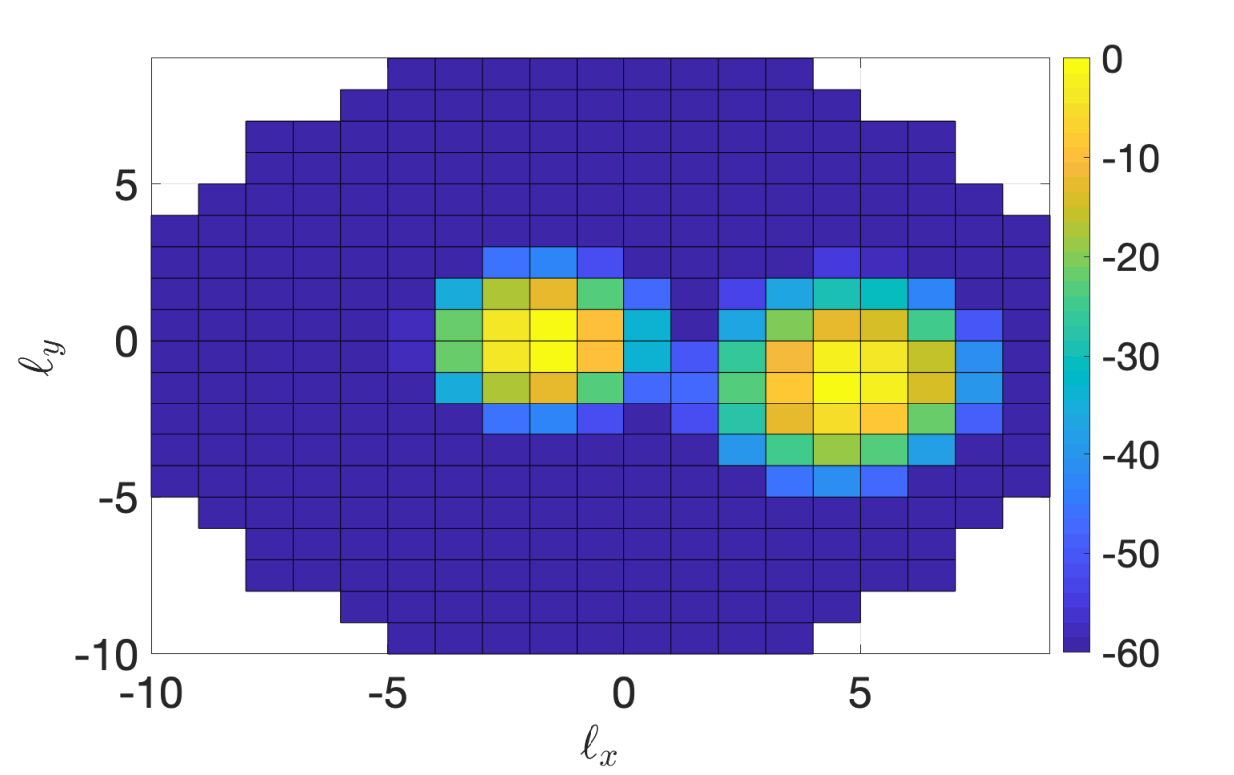
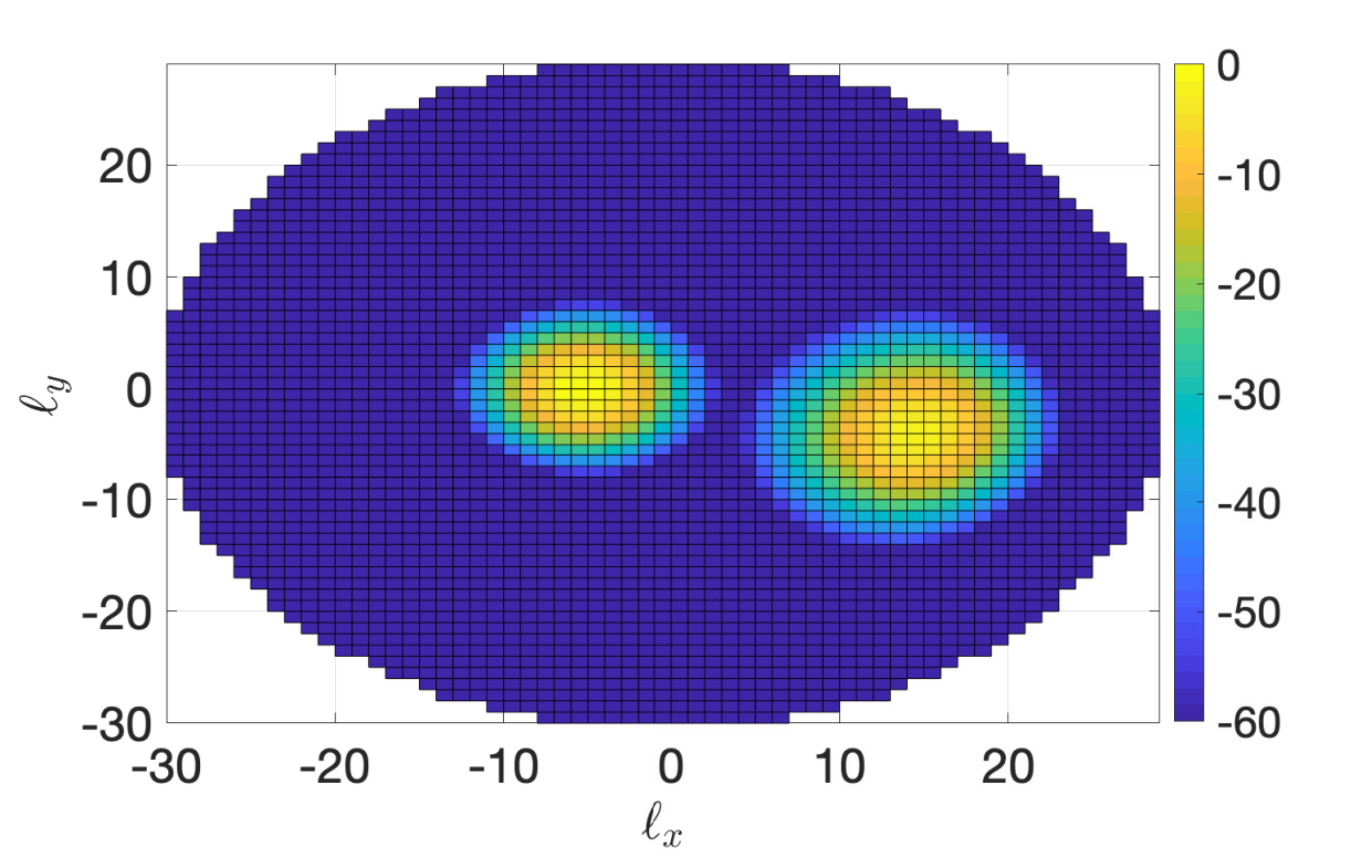
The non-isotropic propagation is considered in Fig. 4. Here, we have $N_{\rm c}=2$ with $\mu_{\theta}=\{30^{\circ},10^{\circ}\}$, $\mu_{\phi}=\{345^{\circ},180^{\circ}\}$ and $\alpha$ such that $\nu^{2}=\{.01,.005\}$, which roughly corresponds to $\sigma_{a}=\{15^{\circ},11^{\circ}\}$. The coupling coefficients are still non-zero within the lattice ellipse $\mathcal{E}_{R}$ in (18) but, unlike Fig. 3, they achieve higher values around the modal directions. Compared to the isotropic case, a reduced number, say ${n_{R}^{\prime}<n_{R}}$, of coupling coefficients is significant. Inspired by the three-sigma rule for Gaussian distributions, $n_{R}^{\prime}$ may be computed as the number of angular sets that are sufficient to capture the $99.7\%$ of the channel power in (26). This yields ${n_{R}^{\prime}=21+14=35}$ and ${n_{R}^{\prime}=145+84=229}$ for Fig. 4(a) and Fig. 4(b), respectively.

Let $h(t)$ be a band-limited stationary random process of bandwidth $B$ that is observed over a time interval $[0,T]$. In the regime $BT\gg 1$, the eigenfunctions of its Karhunen-Loeve expansion approach complex harmonics oscillating at an integer multiple of the fundamental frequency $1/T$. The eigenvalues’ power are obtained by sampling the power spectral density of the process at these frequencies [34, Sec. 3.4]. Next, we show how this fundamental result applies to spatially-stationary electromagnetic fields, which we recall to be band-limited in the spatial-frequency domain with maximum circularly bandwidth $\pi\kappa^{2}$ [3, 12, 31].

Consider the two 2D spatial-frequency Fourier harmonics

with fundamental periods $(r_{x},r_{y})\in\mathcal{R}$ and $(s_{x},s_{y})\in\mathcal{S}$. For any fixed pair $(r_{z},s_{z})$, the discretized plane waves in (21) correspond to two phase-shifted versions of the two 2D spatial-frequency Fourier harmonics, i.e.,

Hence, we can rewrite (21) as (36) where we have defined

Notice that $\widetilde{H}(\ell_{x},\ell_{y},m_{x},m_{y};r_{z},s_{z})$ and $H_{a}(\ell_{x},\ell_{y},m_{x},m_{y})$ are statistically equivalent due to (22). Hence, we can remove the dependance on $r_{z}$ and $s_{z}$ on the spatial correlation function $c({\bf{r}},{\bf{s}})=\mathbb{E}\{h({\bf{r}}+{\bf{r}}^{\prime},{\bf{s}}+{\bf{s}}^{\prime})h^{*}({\bf{r}}^{\prime},{\bf{s}}^{\prime})\}$ of $h({\bf{r}},{\bf{s}})$. By using (36) and (37), it can be approximated as in (38).

References

- [1] A. Pizzo, T. L. Marzetta, and L. Sanguinetti, “Holographic MIMO Communications Under Spatially-Stationary Scattering,” in 2020 54th Asilomar Conference on Signals, Systems, and Computers, 2020, pp. 702–706.
- [2] E. Björnson, L. Sanguinetti, H. Wymeersch, J. Hoydis, and T. L. Marzetta, “Massive MIMO is a reality - what is next?: Five promising research directions for antenna arrays,” Digital Signal Processing, vol. 94, pp. 3 – 20, 2019.
- [3] A. Pizzo, T. L. Marzetta, and L. Sanguinetti, “Spatially-Stationary Model for Holographic MIMO Small-Scale Fading,” IEEE J. Sel. Areas Commun., vol. 38, no. 9, pp. 1964–1979, 2020.
- [4] S. Hu, F. Rusek, and O. Edfors, “Beyond Massive MIMO: The potential of data transmission with large intelligent surfaces,” IEEE Trans. Signal Proc., vol. 66, no. 10, May 2018.
- [5] Q. Wu and R. Zhang, “Intelligent Reflecting Surface Enhanced Wireless Network via Joint Active and Passive Beamforming,” IEEE Trans. Wireless Commun., vol. 18, no. 11, pp. 5394–5409, 2019.
- [6] D. Dardari and N. Decarli, “Holographic Communication Using Intelligent Surfaces,” IEEE Communications Magazine, vol. 59, no. 6, pp. 35–41, 2021.
- [7] T. K. Sarkar, Z. Ji, K. Kim, A. Medouri, and M. Salazar-Palma, “A survey of various propagation models for mobile communication,” IEEE Antennas and Propagation Magazine, vol. 45, no. 3, pp. 51–82, 2003.
- [8] T. L. Marzetta, “Spatially-stationary propagating random field model for Massive MIMO small-scale fading,” in 2018 IEEE Int. Symposium Inf. Theory (ISIT), June 2018, pp. 391–395.
- [9] M. Gustafsson and S. Nordebo, “Characterization of MIMO Antennas Using Spherical Vector Waves,” IEEE Trans. Antennas Propag., vol. 54, no. 9, pp. 2679–2682, 2006.
- [10] A. A. Glazunov, M. Gustafsson, A. F. Molisch, F. Tufvesson, and G. Kristensson, “Spherical Vector Wave Expansion of Gaussian Electromagnetic Fields for Antenna-Channel Interaction Analysis,” IEEE Trans. Antennas Propag., vol. 57, no. 7, pp. 2055–2067, 2009.
- [11] A. A. Glazunov, M. Gustafsson, A. F. Molisch, and F. Tufvesson, “Physical modelling of multiple-input multiple-output antennas and channels by means of the spherical vector wave expansion,” IET Microwaves, Antennas and Propagation, vol. 4, pp. 778–791(13), June 2010.
- [12] A. Pizzo, L. Sanguinetti, and T. L. Marzetta, “Spatial Characterization of Electromagnetic Random Channels,” CoRR, vol. abs/2103.15666, 2021. Online: https://arxiv.org/abs/2103.15666.
- [13] A. S. Y. Poon, D. N. C. Tse, and R. W. Brodersen, “Impact of scattering on the capacity, diversity, and propagation range of multiple-antenna channels,” IEEE Trans. Inf. Theory, vol. 52, no. 3, March 2006.
- [14] A. M. Sayeed, “Deconstructing multiantenna fading channels,” IEEE Trans. Signal Process., vol. 50, no. 10, 2002.
- [15] V. V. Veeravalli, Y. Liang, and A. M. Sayeed, “Correlated MIMO Wireless Channels: Capacity, Optimal Signaling, and Asymptotics,” IEEE Trans. Inf. Theory, vol. 51, no. 6, pp. 2058–2072, 2005.
- [16] A. S. Y. Poon, R. W. Brodersen, and D. N. C. Tse, “Degrees of freedom in multiple-antenna channels: a signal space approach,” IEEE Trans. Inf. Theory, vol. 51, no. 2, pp. 523–536, Feb 2005.
- [17] R. A. Kennedy, P. Sadeghi, T. D. Abhayapala, and H. M. Jones, “Intrinsic Limits of Dimensionality and Richness in Random Multipath Fields,” IEEE Trans. Signal Proc., vol. 55, no. 6, pp. 2542–2556, 2007.
- [18] T. S. Pollock, T. D. Abhayapala, and R. A. Kennedy, “Spatial Limits to MIMO Capacity in General Scattering Environments,” in th International symposium on DSP Communication Systems (DSPCS03), 2003, vol. 1, pp. 49–54.
- [19] E. Björnson, J. Hoydis, and L. Sanguinetti, Massive MIMO Networks: Spectral, Energy, and Hardware Efficiency, vol. 11, Foundations and Trends in Signal Processing, 2017.
- [20] C. A Balanis, Antenna Theory: Analysis and Design, Wiley-Interscience, 4 edition, 2005.
- [21] M. Franceschetti, M. D. Migliore, P. Minero, and F. Schettino, “The Information Carried by Scattered Waves: Near-Field and Nonasymptotic Regimes,” IEEE Trans. Antennas Propag., vol. 63, no. 7, pp. 3144–3157, 2015.
- [22] Y. Xing and T. S. Rappaport, “Propagation Measurements and Path Loss Models for sub-THz in Urban Microcells,” CoRR, vol. abs/2103.01151, 2021. Online:https://arxiv.org/abs/2103.01151.
- [23] H. Weyl, “Ausbreitung elektromagnetischer Wellen über einem ebenen Leiter,” Annalen der Physik, vol. 365, no. 21, pp. 481–500, 1919.
- [24] W. C. Chew, Waves and Fields in Inhomogenous Media, Wiley-IEEE Press, 1995.
- [25] T. B. Hansen and A. D. Yaghjian, Plane-Wave Theory of Time-Domain Fields, Wiley-IEEE Press, New York, 1999.
- [26] D. S. Saxon, “Tensor Scattering Matrix for the Electromagnetic Field,” Phys. Rev., vol. 100, pp. 1771–1775, Dec 1955.
- [27] M. Nieto-Vesperinas and E. Wolf, “Generalized Stokes reciprocity relations for scattering from dielectric objects of arbitrary shape,” Journal of The Optical Society of America A-optics Image Science and Vision, vol. 3, pp. 2038–2046, 1986.
- [28] T. L. Marzetta, “BLAST Arrays of Polarimetric Antennas,” ITD-01-41984K, Nokia Proprietary, 10 05 2001.
- [29] A. Pizzo, T. L. Marzetta, and L. Sanguinetti, “Degrees of Freedom of Holographic MIMO Channels,” in 2020 IEEE 21st Int. Workshop Signal Process. Adv. Wireless Commun. (SPAWC), 2020, pp. 1–5.
- [30] R. W. Heath Jr. and A. Lozano, Foundations of MIMO Communication, Cambridge University Press, 2018.
- [31] A. Pizzo, A. de J. Torres, L. Sanguinetti, and T. L. Marzetta, “Nyquist-Sampling and Degrees of Freedom of Electromagnetic Fields,” CoRR, vol. abs/2109.10040, 2021. Online: https://arxiv.org/abs/2109.10040.
- [32] M. Franceschetti, Wave Theory of Information, Cambridge University Press, 2017.
- [33] D. A. B. Miller, “Communicating with waves between volumes: evaluating orthogonal spatial channels and limits on coupling strengths,” Appl. Opt., vol. 39, no. 11, pp. 1681–1699, Apr 2000.
- [34] H. L. Van Trees, Detection Estimation and Modulation Theory, Part I, Wiley, 1968.
- [35] A. M. Tulino, A. Lozano, and S. Verdu, “Impact of antenna correlation on the capacity of multiantenna channels,” IEEE Trans. Inf. Theory, vol. 51, no. 7, pp. 2491–2509, July 2005.
- [36] M. Franceschetti, “On Landau’s eigenvalue theorem and information cut-sets,” IEEE Trans. Inf. Theory, vol. 61, no. 9, 2015.
- [37] W. Weichselberger, M. Herdin, H. Ozcelik, and E. Bonek, “A stochastic MIMO channel model with joint correlation of both link ends,” IEEE Trans. Wireless Commun., vol. 5, no. 1, pp. 90–100, Jan 2006.
- [38] E. Björnson and L. Sanguinetti, “Rayleigh Fading Modeling and Channel Hardening for Reconfigurable Intelligent Surfaces,” CoRR, vol. abs/2009.04723, 2020. Online: https://arxiv.org/abs/2009.04723.
- [39] A. F. Molisch and X. Zhang, “FFT-based Hybrid Antenna Selection Schemes for Spatially Correlated MIMO Channels,” IEEE Commun. Letters, vol. 8, no. 1, pp. 36–38, 2004.
- [40] Y. Zeng and R. Zhang, “Millimeter wave MIMO with lens antenna array: A new path division multiplexing paradigm,” IEEE Trans. Commun., vol. 64, no. 4, pp. 1557–1571, 2016.
- [41] M. D. Migliore, “On electromagnetics and information theory,” IEEE Trans. Antennas Propag., vol. 56, no. 10, pp. 3188–3200, 2008.
- [42] T. L. Marzetta, “Fundamental Limitations on the Capacity of Wireless Links that use Polarimetric Antenna Arrays,” in Proceedings IEEE International Symposium on Information Theory,, 2002, pp. 51–.
- [43] T. Laas, J. A. Nossek, and W. Xu, “Limits of Transmit and Receive Array Gain in Massive MIMO,” in 2020 IEEE Wireless Communications and Networking Conference (WCNC), 2020, pp. 1–8.