跳到论文正文
W Papers独立论文阅读器 arXiv:2105.01436 论文正文 计算阅读时间 · 0%
引用这篇论文根据当前论文元数据生成,正式投稿前建议核对。


License: arXiv.org perpetual non-exclusive license
arXiv:2105.01436v2 [hep-th] 17 Aug 2021

Gravitational Positivity Bounds on Scalar Potentials

Toshifumi Noumi Affiliation: Department of Physics, Kobe University, Kobe 657-8501, Japan    Junsei Tokuda Affiliation: Department of Physics, Kobe University, Kobe 657-8501, Japan
Abstract

We derive constraints on scalar field theories coupled to gravity by using recently developed positivity bounds in the presence of gravity. It is found that a canonically-normalized real scalar cannot have an arbitrarily flat potential unless some new physics enters well below the Planck scale. An upper bound on the scale of new physics is determined by loop corrections to the self-energy. Our result provides a swampland condition for scalar potentials.

I I. Introduction

Scalar fields play an important role in various contexts of physics. In particle physics, the Higgs boson is a key ingredient of the Standard Model. In cosmology, we need the inflaton to realize the early universe inflation. More theoretically, moduli fields are crucial to understand the Landscape of quantum field theory models. In these contexts, it is important to clarify what kind of scalar potentials have a consistent ultraviolet (UV) completion, especially in the presence of gravity.

A starting point in this direction is the widely accepted statement that quantum gravity prohibits exact global symmetries and so completely flat potentials are not allowed Banks and Dixon 1988; Banks and Seiberg 2011; Harlow and Ooguri 2018. Then, the question is how one can formulate more quantitative constraints useful for phenomenology. Indeed, several bounds on scalar potentials have been proposed in the Swampland Program Vafa 2005 with various degrees of rigors and motivations Ooguri and Vafa 2007; Arkani-Hamed et al. 2007; Palti 2017; Obied et al. 2018; Garg and Krishnan 2019; Ooguri et al. 2019; Gonzalo and Ibáñez 2019; Benakli et al. 2020; Gonzalo and Ibáñez 2020 (see also Palti 2019; van Beest et al. 2021 for reviews). The conjectured bounds, if true, have interesting implications for particle physics and cosmology, which motivates further studies toward their derivation.

In this paper, we explore quantum gravity constraints on scalar potentials in light of recently developed gravitational positivity bounds Hamada et al. 2019; Tokuda et al. 2020; Herrero-Valea et al. 2020. In non-gravitational theories, it is well-known that Wilson coefficients of low-energy effective field theories (EFTs) have to satisfy an infinite set of inequalities called positivity bounds in order to have a standard UV completion Adams et al. 2006. While its extension to gravitational theories has been non-trivial due to the graviton tt-channel pole, the conditions under which (approximate) positivity bounds should hold are clarified by recent works Hamada et al. 2019; Tokuda et al. 2020; Herrero-Valea et al. 2020 (see Bellazzini et al. 2019; Alberte et al. 2020a; Caron-Huot et al. 2021 for related discussions). Following this, we study a real scalar coupled to gravity in 4 dimensions,

ℒ=Mpl22​R−12​(∂ϕ)2−V⁡(ϕ)+ℒhigher+⋯,\mathcal{L}=\frac{M_{\rm pl}^{2}}{2}R-\frac{1}{2}(\partial\phi)^{2}-V(\phi)+\mathcal{L}_{\rm higher}+\cdots\,, (1)

and use the gravitational positivity bounds to derive constraints on the scalar potential V⁡(ϕ)V(\phi) and the higher derivative terms ℒhigher\mathcal{L}_{\rm higher}, clarifying assumptions and limitation of its applicability. Here, RR and MplM_{\rm pl} denote Ricci scalar and the reduced Planck mass, respectively.

II II. Gravitational positivity bounds

In this study, we assume a weakly-coupled UV completion of gravity, whose illustrative example is perturbative string theory. The scattering amplitude will be then unitary and analytic order by order in perturbative expansions in terms of MplM_{\rm pl}. Below, we simply write the ϕ​ϕ→ϕ​ϕ\phi\phi\to\phi\phi scattering amplitude up to 𝒪⁡(Mpl−2)\mathcal{O}(M_{\rm pl}^{-2}) as ℳ⁡(s,t)\mathcal{M}(s,t). Here, (s,t,u)(s,t,u) are Mandelstam variables satisfying s+t+u=4​mph2s+t+u=4m_{\rm ph}^{2}, where mph2m_{\rm ph}^{2} is the pole mass of ϕ\phi. We assume that ℳ⁡(s,t<0)\mathcal{M}(s,t<0) is analytic in the complex ss-plane except for discontinuities across the real ss-axis, and it behaves mildly at high energies to satisfy |ℳ⁡(s,t<0)/s2|→0|\mathcal{M}(s,t<0)/s^{2}|\to 0 in the limit |s|→∞|s|\to\infty (tt: fixed). 11 1 In gapped systems, this mild behavior follows from the polynomial boundedness assumption Froissart 1961; Martin 1963 in combination with the Phragmén-Lindelöf theorem. Positivity bounds in the absence of the polynomial boundedness assumption are discussed in Tokuda 2019. Then, the s,us,u-channel pole subtracted amplitude ℳ~​(s,t)≔ℳ⁡(s,t)−(s,u​-poles)\widetilde{\mathcal{M}}(s,t)\coloneqq\mathcal{M}(s,t)-(s,u\text{-poles}) also satisfies the same properties. These assumptions lead to the relation (see also FIG. 1)

−∫𝒞rd​s′2​π​iℳ~​(s′,t)(s′−s∗)3=∫𝒞1+𝒞2d​s′2​π​iℳ~​(s′,t)(s′−s∗)3fort<0,-\int_{\mathcal{C}_{r}}\frac{\mathrm{d}s^{\prime}}{2\pi i}\frac{\widetilde{\mathcal{M}}(s^{\prime},t)}{\left(s^{\prime}-s_{*}\right)^{3}}=\int_{\mathcal{C}_{1}+\mathcal{C}_{2}}\frac{\mathrm{d}s^{\prime}}{2\pi i}\frac{\widetilde{\mathcal{M}}(s^{\prime},t)}{\left(s^{\prime}-s_{*}\right)^{3}}\quad\text{for}\,t<0\,, (2)

where s∗=2​mph2−(t/2)+i​μs_{*}=2m_{\rm ph}^{2}-(t/2)+i\mu and μ>0\mu>0. The contour 𝒞r\mathcal{C}_{r} is a semi-circle centered at s=s∗s=s_{*} with a radius rr. The contours 𝒞1\mathcal{C}_{1} and 𝒞2\mathcal{C}_{2} are straight lines defined by 𝒞1≔{s′|−∞+i​μ<s′<s∗−r}\mathcal{C}_{1}\coloneqq\bigl\{s^{\prime}|\,-\infty+i\mu<s^{\prime}<s_{*}-r\bigr\} and 𝒞2≔{s′|s∗+r<s′<∞+i​μ}\mathcal{C}_{2}\coloneqq\bigl\{s^{\prime}|\,s_{*}+r<s^{\prime}<\infty+i\mu\bigr\}, respectively. Next, we consider the low-energy expansion, ℳ~​(s,t)=∑n=0∞cn​(t,μ)n!​(s−s∗)n+(t​-poles)\widetilde{\mathcal{M}}(s,t)=\sum_{n=0}^{\infty}\frac{c_{n}(t;\mu)}{n!}\left(s-s_{*}\right)^{n}+(t\text{-poles}). The residue of poles are polynomials and particularly we have ∂s2Rest=0​ℳ=−2​Mpl−2\partial_{s}^{2}{\rm Res}_{t=0}\mathcal{M}=-2M_{\rm pl}^{-2}, Rest=0​ℳ{\rm Res}_{t=0}\mathcal{M} being the residue of the graviton tt-channel pole. This reflects the spin-2 nature of graviton. The real part of eq. (2) in the limit r→+0r\to+0 then gives

Re​c2​(t,μ)=32π​𝐏​∫0∞d​s′​Im​ℳ~s​(s′+i​μ,t)(s′−u′)3+2Mpl2​t\mathrm{Re}\,c_{2}(t;\mu)=\frac{32}{\pi}{\bf P}\int^{\infty}_{0}\mathrm{d}s^{\prime}\frac{\mathrm{Im}\,\widetilde{\mathcal{M}}_{s}(s^{\prime}+i\mu,t)}{\left(s^{\prime}-u^{\prime}\right)^{3}}+\frac{2}{M_{\rm pl}^{2}t} (3)

for t<0t<0. Here, u′≔4​mph2−s′−tu^{\prime}\coloneqq 4m_{\rm ph}^{2}-s^{\prime}-t and 𝐏{\bf P} denoting the Cauchy principal value. We decomposed Im​ℳ~\mathrm{Im}\,\widetilde{\mathcal{M}} into the ss- and uu-channel pieces as Im​ℳ~​(s,t)=Im​ℳ~s​(s,t)+Im​ℳ~u​(s,t)\mathrm{Im}\,\widetilde{\mathcal{M}}(s,t)=\mathrm{Im}\,\widetilde{\mathcal{M}}_{s}(s,t)+\mathrm{Im}\,\widetilde{\mathcal{M}}_{u}(s,t) for t<0t<0, and imposed the s↔us\leftrightarrow u crossing symmetry as Im​ℳ~u​(u,t)=Im​ℳ~s​(s,t)\mathrm{Im}\,\widetilde{\mathcal{M}}_{u}(u,t)=\mathrm{Im}\,\widetilde{\mathcal{M}}_{s}(s,t).

Figure 1: Analytic structure of ℳ~​(s,t)\widetilde{\mathcal{M}}(s,t) on the complex ss-plane and the integration contour to derive the relation (2). The wavy line is a brunch cut and the point s=s∗s=s_{*} is the reference point. We choose s∗=2​mph2−(t/2)+i​μs_{*}=2m_{\rm ph}^{2}-(t/2)+i\mu (μ>0\mu>0).

We also used Im​ℳ~s​(s,t)=0\mathrm{Im}\,\widetilde{\mathcal{M}}_{s}(s,t)=0 for s<0s<0. One can evaluate the integral of Im​ℳ~s​(s′,t)\mathrm{Im}\,\widetilde{\mathcal{M}}_{s}(s^{\prime},t) at low energy regions s′<Λth2s^{\prime}<\Lambda_{\rm th}^{2} within EFT Bellazzini 2017; de Rham et al. 2017 to improve (3) as22 2 An importance of the improvement procedure done in (4) to obtain non-trivial constraints on EFTs in the gravitational setups has been found recently in Alberte et al. 2020a; Alberte et al. 2020b.

c2,impr​(t)\displaystyle c_{2,\,{\rm impr}}(t) ≔Re​c2​(t,ϵ)−32π​𝐏​∫0Λth2d​s′​Im​ℳ~s​(s′+i​ϵ,t)(s′−u′)3\displaystyle\coloneqq\mathrm{Re}\,c_{2}(t;\epsilon)-\frac{32}{\pi}{\bf P}\int^{\Lambda_{\rm th}^{2}}_{0}\mathrm{d}s^{\prime}\,\frac{\mathrm{Im}\,\widetilde{\mathcal{M}}_{s}(s^{\prime}+i\epsilon,t)}{\left(s^{\prime}-u^{\prime}\right)^{3}}
=32π​∫Λth2∞d​s′​Im​ℳ~s​(s′+i​ϵ,t)(s′−u′)3+2Mpl2​t,\displaystyle=\frac{32}{\pi}\int^{\infty}_{\Lambda_{\rm th}^{2}}\mathrm{d}s^{\prime}\,\frac{\mathrm{Im}\,\widetilde{\mathcal{M}}_{s}(s^{\prime}+i\epsilon,t)}{\left(s^{\prime}-u^{\prime}\right)^{3}}+\frac{2}{M_{\rm pl}^{2}t}\,, (4)

where ϵ\epsilon is an infinitesimal positive constant and Λth\Lambda_{\rm th} denotes a threshold scale above which the EFT evaluation of ℳ\mathcal{M} is unreliable: e.g., we have Λth≲Λ\Lambda_{\rm th}\lesssim\Lambda when considering a model with a term (∂ϕ)4/Λ4(\partial\phi)^{4}/\Lambda^{4}. We assume Λth2≫mph2\Lambda_{\rm th}^{2}\gg m_{\rm ph}^{2} throughout this study. The second term on the right-hand side (RHS) of (4) diverges as −∞-\infty in the limit t→−0t\to-0. This makes the positivity of c2,impr​(0)c_{2,\,{\rm impr}}(0) unclear. In Tokuda et al. 2020, the cancellation of 𝒪⁡(t−1)\mathcal{O}(t^{-1}) terms on the RHS of (4) is explicitly demonstrated by assuming the Regge behavior 33 3 If we go beyond the 𝒪⁡(Mpl−2)\mathcal{O}(M_{\rm pl}^{-2}) analysis, the 𝒪⁡(ln−1⁡(s/Ms2))\mathcal{O}(\ln^{-1}(s/M_{\rm s}^{2})) sub-leading correction to the Regge behavior plays an important role as discussed in Herrero-Valea et al. 2020. Also, we suppressed the positive contributions from other states which are irrelevant for the Reggeization of tt-channel graviton exchange in (5).

Im​ℳ~s​(s,t)≃f⁡(t)​(sMs2)2+j⁡(t)​[1+𝒪⁡(Ms2s)]+⋯,\mathrm{Im}\,\widetilde{\mathcal{M}}_{s}(s,t)\simeq f(t)\left(\frac{s}{M_{\rm s}^{2}}\right)^{2+j(t)}\left[1+\mathcal{O}\left(\frac{M_{\rm s}^{2}}{s}\right)\right]+\cdots\,, (5)

at s≫Ms2s\gg M_{\rm s}^{2}, where f⁡(t)f(t) and j⁡(t)j(t) are functions regular in the vicinity of t=0t=0. A scale MsM_{\rm s} denotes the lightest mass scale of the heavy physics which Reggeizes the amplitude. An explicit computation of the 𝒪⁡(t0)\mathcal{O}(t^{0}) terms shows Tokuda et al. 2020

c2,impr​(0)>−𝒪⁡(1)Mpl2​Ms2,c_{2,\,{\rm impr}}(0)>-~\frac{\mathcal{O}(1)}{M_{\rm pl}^{2}M_{\rm s}^{2}}\,, (6)

assuming the single scaling j′∼|j′′/j′|∼|f′/f|≲𝒪⁡(Ms−2)j^{\prime}\sim|j^{\prime\prime}/j^{\prime}|\sim|f^{\prime}/f|\lesssim\mathcal{O}(M_{\rm s}^{-2}) which is the case in tree-level amplitudes in perturbative string theory with MsM_{\rm s} being the string scale. Here, the prime denotes the tt-derivative evaluated at t=0t=0. 44 4 A similar order estimate of approximate positivity can be found in Hamada et al. 2019; Loges et al. 2020. A proof of the single scaling is beyond the scope of this paper. The bound (6) is distinct from the one conjectured in Alberte et al. 2020a; Alberte et al. 2020b which depends on the EFT cutoff scales or mass scales of fields in EFTs. Although the precise value of the RHS of (6) will depend on the details of UV completion, this approximate positivity provides non-trivial constraints on EFTs as we shall see below.

III III. Bounds on scalar theories coupled to gravity

III.1 A. Setup

Based on an inequality (6), we shall derive a bound on a real scalar field theory coupled to gravity whose classical Lagrangian is given by eq. (1), with classical potential V⁡(ϕ)V(\phi) and higher derivative terms ℒhigher\mathcal{L}_{\rm higher} of the form

V⁡(ϕ)=m2​ϕ22+g​ϕ33!+λ​ϕ44!+⋯,\displaystyle V(\phi)=\frac{m^{2}\phi^{2}}{2}+\frac{g\phi^{3}}{3!}+\frac{\lambda\phi^{4}}{4!}+\cdots\,,
ℒhigher=α​(∂ϕ)48​Λ4+⋯,\displaystyle\mathcal{L}_{\rm higher}=\frac{\alpha(\partial\phi)^{4}}{8\Lambda^{4}}+\cdots,

where α\alpha is a constant of order unity. Ellipses stand for higher order non-renormalizable terms which are present in general in the classical action because we regard this system as an EFT. Our choice of ℒhigher\mathcal{L}_{\rm higher} is necessary and sufficient for taking into account the influence of higher derivative corrections on positivity bounds up to 𝒪⁡(Λ−4)\mathcal{O}(\Lambda^{-4}), thanks to the invariance of ℳ\mathcal{M} under perturbative field redefinitions.

We require |g/m|,|λ|≲1|g/m|,\,|\lambda|\lesssim 1 to ensure the perturbative expansion of ℳ\mathcal{M} in terms of coupling constants. We also require that the minimum of V⁡(ϕ)V(\phi) is located at ϕ=0\phi=0 at least within the range |ϕ|≲Λth|\phi|\lesssim\Lambda_{\rm th} to justify the perturbative evaluations of ℳ⁡(s,t)\mathcal{M}(s,t) up to s≲Λth2s\lesssim\Lambda_{\rm th}^{2}.

We use the dimensional regularization to regulate UV divergences and adopt the MS¯\overline{{\rm MS}} scheme except we determine the counterterm of the form Y​ϕY\phi by imposing ⟨ϕ⟩=0\langle\phi\rangle=0 (see appendices for details).

Figure 2: Diagrams (i): Relevant 1PI diagrams for an effective vertex ϕ2​h\phi^{2}h in the present analysis. Solid lines and double wavy lines denote the propagators of ϕ\phi and hμ​νh_{\mu\nu}, respectively. Diagrams (ii): The tt-channel diagrams which give negative contributions to c2,impr​(0)c_{2,\,{\rm impr}}(0), expressed in terms of the 1PI vertices shown in the diagrams (i).

III.2 B. General bound

We compute c2,impr​(0)c_{2,\,{\rm impr}}(0). We may decompose c2,impr​(0)c_{2,\,{\rm impr}}(0) into the non-gravitational piece and the gravitational piece, c2,impr​(0)=cnon-grav+cgravc_{2,\,{\rm impr}}(0)=c_{\text{non-grav}}+c_{\text{grav}}. Diagrams without gravitons and those with gravitons contribute to cnon-gravc_{\text{non-grav}}, and cgravc_{\text{grav}}, respectively. We start with the non-gravitational one. The contributions from non-renormalizable terms such as α​(∂ϕ)4/(8​Λ4)\alpha(\partial\phi)^{4}/(8\Lambda^{4}) and ϕ6/Λ2\phi^{6}/\Lambda^{2} can be written as α~/Λ4\tilde{\alpha}/\Lambda^{4}. We have α~=α\tilde{\alpha}=\alpha when considering a renormalizable potential. Renormalizable interactions also contribute to cnon-gravc_{\text{non-grav}} via s,us,u-channel one-loop diagrams. Referring to the latter contributions as cnon​-​grav,renc_{{\rm non\text{-}grav,\,ren}}, we have cnon-grav=α~Λ4+cnon​-​grav,renc_{\text{non-grav}}=\frac{\tilde{\alpha}}{\Lambda^{4}}+c_{{\rm non\text{-}grav,\,ren}} with

cnon​-​grav,ren≃λ216​π2​Λth4+g412​π2​m2​Λth6\displaystyle c_{{\rm non\text{-}grav,\,ren}}\simeq\frac{\lambda^{2}}{16\pi^{2}\Lambda_{\rm th}^{4}}+\frac{g^{4}}{12\pi^{2}m^{2}\Lambda_{\rm th}^{6}}
−λ​g26​π2​Λth6​(ln⁡(Λth2m2)−16).\displaystyle\qquad\qquad\qquad-\frac{\lambda g^{2}}{6\pi^{2}\Lambda_{\rm th}^{6}}\left(\ln\left(\frac{\Lambda_{\rm th}^{2}}{m^{2}}\right)-\frac{1}{6}\right)\,. (7)

When ϕ\phi is a shift symmetric scalar, one can always make cnon-gravc_{\text{non-grav}} positive by choosing α>0\alpha>0, the coefficient of the higher derivative term (∂ϕ)4(\partial\phi)^{4}. This is reminiscent of the conventional positivity bound without gravity.

The presence of the gravitational piece cgravc_{\text{grav}} changes the story, however. In particular, loop corrections to the graviton tt-channel exchange diagram give rise to negative contributions to which we refer as cgrav,t​-​chc_{{\rm grav},\,t\text{-}{\rm ch}}: corresponding diagrams are shown in FIG. 2. Note that we are interested in amplitudes up to 𝒪⁡(Mpl−2)\mathcal{O}(M_{\rm pl}^{-2}), so that we can use the tree-level graviton propagator together with the loop-corrected one-particle irreducible (1PI) vertices. 55 5 Note that negative contributions from the tt-channel tree-level graviton exchange have been computed in different setups up to one-loop level Cheung and Remmen 2014; Andriolo et al. 2018; Chen et al. 2019; Alberte et al. 2020a; Alberte et al. 2020b. To compute cgrav,t​-​chc_{{\rm grav},\,t\text{-}{\rm ch}}, we write the 1PI effective action Γ\Gamma as

Γ[ϕ,h]∋−12∫d4​k(2​π)4K(k2)ϕ(k)ϕ(−k)\displaystyle\Gamma[\phi,h]\ni-\frac{1}{2}\int\frac{\mathrm{d}^{4}k}{(2\pi)^{4}}K(k^{2})\phi(k)\phi(-k) (8)
+14∫d4​k1(2​π)4∫d4​k3(2​π)4Vμ​ν(k1,k3)ϕ(k1)ϕ(k3)hμ​ν(q),\displaystyle+\frac{1}{4}\int\frac{\mathrm{d}^{4}k_{1}}{(2\pi)^{4}}\int\frac{\mathrm{d}^{4}k_{3}}{(2\pi)^{4}}V^{\mu\nu}\left(k_{1},k_{3}\right)\phi(k_{1})\phi(k_{3})h_{\mu\nu}(q)\,,

where we suppressed terms irrelevant for our present analysis. Also, gμ​ν=ημ​ν+hμ​νg_{\mu\nu}=\eta_{\mu\nu}+h_{\mu\nu} and qμ≔−(k1+k3)μq^{\mu}\coloneqq-(k_{1}+k_{3})^{\mu}. The kernel K⁡(k2)K(k^{2}) denotes an inverse of a loop-corrected propagator of ϕ\phi, which is written in terms of the self-energy Π⁡(k2)\Pi(k^{2}) as K⁡(k2)=k2+m2−Π⁡(k2)K(k^{2})=k^{2}+m^{2}-\Pi(k^{2}). The 1PI ϕ​ϕ​h\phi\phi h vertex function is denoted by Vμ​ν​(k1,k3)V^{\mu\nu}(k_{1},k_{3}) and we parameterize it with imposing the on-shell conditions k12=k32=−mph2k_{1}^{2}=k_{3}^{2}=-m_{\rm ph}^{2} as

Vμ​ν​(k1,k3)|k12=k32=−mph2=T⁡(q2)​ημ​ν+P⁡(q2)​qμ​qν\displaystyle V^{\mu\nu}(k_{1},k_{3})|_{k_{1}^{2}=k_{3}^{2}=-m_{\rm ph}^{2}}=T(q^{2})\eta^{\mu\nu}+P(q^{2})q^{\mu}q^{\nu}
−2​Q​(q2)​(pμ​qν+pν​qμ)+4​R​(q2)​pμ​pν.\displaystyle\qquad\qquad\quad\!\!-2Q(q^{2})(p^{\mu}q^{\nu}+p^{\nu}q^{\mu})+4R(q^{2})p^{\mu}p^{\nu}\,. (9)

Here, we defined pμ≔(k1−k3)μ/2p^{\mu}\coloneqq(k_{1}-k_{3})^{\mu}/2. For example, at the tree-level approximation, we have Ttree=k1.k3−m2T_{\rm tree}=k_{1}.k_{3}-m^{2}, Ptree=−1/2P_{\rm tree}=-1/2, Qtree=0Q_{\rm tree}=0, and Rtree=1/2R_{\rm tree}=1/2. The final term on the RHS of (9) expresses the transverse-traceless component of hμ​νh_{\mu\nu}, and only this piece contributes to the spin-2 part of the tt-channel graviton exchange diagrams which are represented by the lower diagram of FIG. 2,

ℳ⁡(s,t)|FIG.2=4​R2​(−t)​s​uMpl2​t×Z2+𝒪⁡(s0),\mathcal{M}(s,t)|_{{\rm FIG.~\ref{fig:neg1}}}=\frac{4R^{2}(-t)su}{M_{\rm pl}^{2}t}\times Z^{2}+\mathcal{O}(s^{0})\,, (10)

where we used q2=−tq^{2}=-t and ZZ is the residue of the propagator of ϕ\phi. We then find the relation cgrav,t​-​ch=8​Z2​∂x(R2​(x))|x=0/Mpl2≃8​R′​(0)/Mpl2c_{{\rm grav},\,t\text{-}{\rm ch}}=8Z^{2}\partial_{x}(R^{2}(x))|_{x=0}/M_{\rm pl}^{2}\simeq 8R^{\prime}(0)/M_{\rm pl}^{2} to get

cgrav,t​-​ch≃−45−8​π​31296​π2​g2Mpl2​m4−10−π24608​π4​λ2Mpl2​m2<0.c_{{\rm grav},\,t\text{-}{\rm ch}}\simeq-\frac{45-8\pi\sqrt{3}}{1296\pi^{2}}\frac{g^{2}}{M_{\rm pl}^{2}m^{4}}-\frac{10-\pi^{2}}{4608\pi^{4}}\frac{\lambda^{2}}{M_{\rm pl}^{2}m^{2}}<0\,. (11)

Note that the leading-order contributions from the ϕ4\phi^{4} vertex arise at the two-loop level. 66 6 The appearance of the leading-order term at two-loop level is analogous to the fact that the leading-order correction to the field renormalization appears at two-loop level in λ​ϕ4\lambda\phi^{4} theory. Also note that non-renormalizable terms in V⁡(ϕ)V(\phi), such as ϕ6/Λ2\phi^{6}/\Lambda^{2} vertex, contribute to cgrav,t​-​chc_{{\rm grav},\,t\text{-}{\rm ch}} at 𝒪⁡(Mpl−2​Λ−2)\mathcal{O}(M_{\rm pl}^{-2}\Lambda^{-2}), which are negligible compared to the 𝒪⁡(Λ−4)\mathcal{O}(\Lambda^{-4}) contribution to cnon-gravc_{\text{non-grav}} as long as Λ2≪Mpl2\Lambda^{2}\ll M_{\rm pl}^{2}. Interestingly, each term of (11) can be written in terms of the self-energy Π\Pi as

cgrav,t​-​ch≃−2​[Π′′​(−m2)|λ=0+2​Π′′​(−m2)|g=0]3​Mpl2,c_{{\rm grav},\,t\text{-}{\rm ch}}\simeq-\frac{2\left[\Pi^{\prime\prime}(-m^{2})|_{\lambda=0}+2\Pi^{\prime\prime}(-m^{2})|_{g=0}\right]}{3M_{\rm pl}^{2}}\,, (12)

where unitarity ensures Π′′​(−m2)>0\Pi^{\prime\prime}(-m^{2})>0 because Π⁡(k2)\Pi(k^{2}) satisfies the twice-subtracted dispersion relation at least within the range of our approximation. This implies that negativity of cgrav,t​-​chc_{{\rm grav},\,t\text{-}{\rm ch}} could be related to the physics of the loop-corrected self-energy. Although cgrav,t​-​chc_{{\rm grav},\,t\text{-}{\rm ch}} is determined by the behavior of the vertex ϕ2​h\phi^{2}h when the momentum of an external graviton is soft, it is not fixed by the soft graviton theorem alone: see appendices for details.

Diagrams other than those shown in FIG. 2 also contribute to cgravc_{\text{grav}} at 𝒪⁡(Mpl−2)\mathcal{O}(M_{\rm pl}^{-2}). Such diagrams are the diagrams with s,us,u-channel tree-level graviton exchange diagrams, diagrams with a graviton-scalar conversion, and diagrams with a graviton propagator inside loops. We refer to these contributions as cgrav,othersc_{{\rm grav,\,others}}, which can be evaluated as

cgrav,others∼𝒪⁡((g/m)2Mpl2​Λth2,λMpl2​Λth2),c_{{\rm grav,\,others}}\sim\mathcal{O}\left(\frac{(g/m)^{2}}{M_{\rm pl}^{2}\Lambda_{\rm th}^{2}},\frac{\lambda}{M_{\rm pl}^{2}\Lambda_{\rm th}^{2}}\right)\,, (13)

and we have cgrav=cgrav,t​-​ch+cgrav,othersc_{\text{grav}}=c_{{\rm grav},\,t\text{-}{\rm ch}}+c_{{\rm grav,\,others}}. Practically, the term cgrav,othersc_{{\rm grav,\,others}} can be ignored to read off the implication of the bound. 77 7 This is because the 𝒪⁡((g/m)2/(Mpl2​Λth2))\mathcal{O}\bigl((g/m)^{2}/(M_{\rm pl}^{2}\Lambda_{\rm th}^{2})\bigr) terms are smaller than |cgrav,t​-​ch||c_{{\rm grav},\,t\text{-}{\rm ch}}| by factors of m2/Λth2m^{2}/\Lambda_{\rm th}^{2}, and the 𝒪⁡(λ/(Mpl2​Λth2))\mathcal{O}\bigl(\lambda/(M_{\rm pl}^{2}\Lambda_{\rm th}^{2})\bigr) terms can be comparable to or larger than the 𝒪⁡(λ2/Λth4)\mathcal{O}(\lambda^{2}/\Lambda_{\rm th}^{4}) term contained in cnon​-​grav,renc_{{\rm non\text{-}grav,\,ren}} only when λ/(Mpl2​Λth2)≲𝒪⁡(Mpl−4)\lambda/(M_{\rm pl}^{2}\Lambda_{\rm th}^{2})\lesssim\mathcal{O}(M_{\rm pl}^{-4}). We thus discuss the implications of an inequality,

α~Λ4+cnon​-​grav,ren+cgrav,t​-​ch>−𝒪⁡(1)Mpl2​Ms2.\frac{\tilde{\alpha}}{\Lambda^{4}}+c_{{\rm non\text{-}grav,\,ren}}+c_{{\rm grav},\,t\text{-}{\rm ch}}>\frac{-\,\mathcal{O}(1)}{M_{\rm pl}^{2}M_{\rm s}^{2}}\,. (14)

Each term is given in eqs. (7) and (11). Note that this bound is renormalization scheme independent at least within the range of our approximation. Also, we do not distinguish between mm and mphm_{\rm ph} because the difference comes in at higher orders.

III.3 C. Analysis of the bound

III.3.1 Emergence of a critical scale

The bound (14) is meaningful only when the allowed negativity on the order of Mpl−2​Ms−2M_{\rm pl}^{-2}M_{\rm s}^{-2} is negligible. We introduce a critical energy scale Λ∗\Lambda_{*} as Λ∗≔(−cgrav,t​-​ch)−1/4\Lambda_{*}\coloneqq(-c_{{\rm grav},\,t\text{-}{\rm ch}})^{-1/4}, explicitly given as

Λ∗=(10−π24608​π4​λ2Mpl2​m2+45−8​π​31296​π2​g2Mpl2​m4)−14,\Lambda_{*}=\left(\frac{10-\pi^{2}}{4608\pi^{4}}\frac{\lambda^{2}}{M_{\rm pl}^{2}m^{2}}+\frac{45-8\pi\sqrt{3}}{1296\pi^{2}}\frac{g^{2}}{M_{\rm pl}^{2}m^{4}}\right)^{-\frac{1}{4}}\,, (15)

which is determined by the loop corrections to the self-energy in the present model as indicated by eq. (12). The 𝒪⁡(Mpl−2​Ms−2)\mathcal{O}(M_{\rm pl}^{-2}M_{\rm s}^{-2}) term can be ignored in eq. (14) when the condition

Applicability​Condition:min⁡(Λ,Λ∗)<Mpl​Ms{\rm Applicability\,\,Condition}:\,\,{\rm min}\left(\Lambda,\,\Lambda_{*}\right)<\sqrt{M_{\rm pl}M_{\rm s}} (16)

is satisfied. Under the condition (16), we discuss the implications of gravitational positivity bounds (14). It turns out that implications of (14) are clearly different between the following two cases,

Case⁡(I):Λ∗4≫Λ4,Case⁡(II):Λ∗4≪Λ4.\displaystyle{\rm Case\,(I):}\,\,\Lambda_{*}^{4}\gg\Lambda^{4}\,,\qquad{\rm Case\,(II):}\,\,\Lambda_{*}^{4}\ll\Lambda^{4}\,.

III.3.2 Case (I): Conventional positivity bounds

EFTs fall into this class when new physics appears well below the critical scale Λ∗\Lambda_{*}. The bound (14) on such models is well approximated by

α~Λ4+cnon​-​grav,ren≥0.\frac{\tilde{\alpha}}{\Lambda^{4}}+c_{{\rm non\text{-}grav,\,ren}}\geq 0\,. (17)

As explained below eq. (7), this provides a constraint on non-renormalizable terms such as α​(∂ϕ)4/(8​Λ4)\alpha(\partial\phi)^{4}/(8\Lambda^{4}), and is the same as the conventional positivity bound without gravity. This is in accord with the decoupling of low-energy physics from the physics of quantum gravity.
Refer to caption
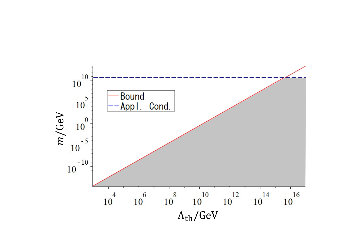
Figure 3: Gravitational positivity bound on λ​ϕ4\lambda\phi^{4} theory. Lines saturating our bound (18) and the applicability condition (16) in λ​ϕ4\lambda\phi^{4} theory are shown in the solid red line and dashes blue line, respectively. We substitute Ms=1016​GeVM_{\rm s}=10^{16}{\rm GeV} and λ=10−2\lambda=10^{-2} to draw the dashed lines. The shaded region is excluded by the bound (18) under the condition (20).

III.3.3 Case (II): Bounds on scalar potentials

EFTs fall into this class when new physics appears well above the critical scale Λ∗\Lambda_{*}. The bound (14) on such EFTs reads

cnon​-​grav,ren−1Λ∗4≥0.c_{{\rm non\text{-}grav,\,ren}}-\frac{1}{\Lambda_{*}^{4}}\geq 0\,. (18)

The left-hand side (LHS) of (18) is determined once V⁡(ϕ)V(\phi) is given, and hence eq. (18) constrains the potential V⁡(ϕ)V(\phi). This is a genuinely new bound which is distinct from the ordinary positivity bound without gravity. The new bound (18) typically prohibits an arbitrarily flat potential: for instance, in λ​ϕ4\lambda\phi^{4} theory, eq. (18) gives a lower bound on m2m^{2} for fixed Λth\Lambda_{\rm th},

m≥10−π2288​π2​Λth2Mpl≈2.8×10⁹​(Λth1015​GeV)2​GeV,m\geq\sqrt{\frac{10-\pi^{2}}{288\pi^{2}}}\frac{\Lambda_{\rm th}^{2}}{M_{\rm pl}}\approx 2.8\times 10^{9}\left(\frac{\Lambda_{\rm th}}{10^{15}\,{\rm GeV}}\right)^{2}\,\,{\rm GeV}\,, (19)

while the applicability condition (16) reads

m<5.4×10¹²​λ​(Ms1016​GeV)GeV.m<5.4\times 10^{12}\lambda\,\left(\frac{M_{\rm s}}{10^{16}\,{\rm GeV}}\right)\quad{\rm GeV}\,. (20)

Lines saturating eqs. (19) and (20) are plotted in the (m,Λth)(m,\,\Lambda_{\rm th})-plane in FIG. 3. We find that the mass of the scalar field cannot be arbitrarily light in λ​ϕ4\lambda\phi^{4} theory. In the presence of the cubic interaction, the expression of the bound (18) is complicated, but it is obvious that tiny mass is prohibited for fixed λ\lambda and g/mg/m. In particular, when having the scaling g2≲|λ|​m2g^{2}\lesssim|\lambda|m^{2}, the bound (18) reads

m≳Λth2Mpl​[1.8×10⁻²​(g/m)2λ2+4.6×10−5]1/2,m\gtrsim\frac{\Lambda_{\rm th}^{2}}{M_{\rm pl}}\left[\frac{1.8\times 10^{-2}~(g/m)^{2}}{\lambda^{2}}+4.6\times 10^{-5}\right]^{1/2}\,, (21)

non-trivially constraining V⁡(ϕ)V(\phi) for a given cutoff Λth\Lambda_{\rm th}.

III.4 D. Summary of the results

To summarize, scalar potentials cannot be arbitrarily flat to be consistent with the gravitational positivity bound: for example, we cannot tune the mass to be arbitrarily smaller than the cutoff scale Λth\Lambda_{\rm th} without violating the bound (18). Our result provides a quantitative swampland condition for scalar potentials which can be derived under several clear assumptions.

Any scalar field theory coupled to gravity which violates the bound (18) has to possess appropriate non-renormalizable terms such as α​(∂ϕ)4/(8​Λ4)\alpha(\partial\phi)^{4}/(8\Lambda^{4}) with Λ≲Λ∗\Lambda\lesssim\Lambda_{*} and α>0\alpha>0, in order to satisfy the bound (14). The presence of such non-renormalizable terms can be interesting phenomenologically. This is one of the main result of this study.

As a caveat, we remark however that our bound (14) still has a room to accommodate models with a very tiny scalar mass. One can take the shift symmetric limit of a given massive scalar theory without violating the bound (14) by requiring Λ∗≫min⁡(Λ,Mpl​Ms)\Lambda_{*}\gg{\rm min}(\Lambda,\,\sqrt{M_{\rm pl}M_{\rm s}}). 88 8 Such a consistent shift symmetric limit can be explicitly realized in a model of a light scalar field whose tiny mass is protected by some symmetry. For instance, we consider the model of complex scalar Φ\Phi in which the approximate global U⁡(1)U(1) symmetry is spontaneously broken, ℒ=−|∂Φ|2−g4​(|Φ|2−v22)2+g​v2​ϵ2​(Φ2+Φ∗2),\displaystyle\mathcal{L}=-\left|\partial\Phi\right|^{2}-\frac{g}{4}\left(|\Phi|^{2}-\frac{v^{2}}{2}\right)^{2}+\frac{gv^{2}\epsilon}{2}\left(\Phi^{2}+{\Phi^{*}}^{2}\right)\,, with g>0g>0, v≠0v\neq 0, and 0<ϵ≪10<\epsilon\ll 1. One can check that the ϵ→0\epsilon\to 0 limit provides a consistent shift symmetric limit for the pseudo Nambu-Goldstone boson. For instance, a consistent shift symmetric limit of λ​ϕ4\lambda\phi^{4} theory is λ,m2→0\lambda,m^{2}\to 0 with satisfying |λ/m|→0|\lambda/m|\to 0. It would be interesting if one could sharpen our analysis further to exclude all the flat potentials.

IV IV. Illustrative examples

As an important application, we firstly discuss an implication of the bound (18) to the renormalizable potential of the Higgs boson in the Standard Model. We then discuss more general form of potentials with non-renormalizable terms which have been frequently discussed in cosmology. We will consider axion-like particle models and the Starobinsky inflation as illustrative examples of non-renormalizable potentials.

IV.1 A. Renormalizable potential: Higgs boson

Let us consider the implication of (18) to the Higgs potential. The classical potential for the Higgs boson ϕ\phi in the unitary gauge is parametrized as m∼125m\sim 125 GeV, g/m∼1.5g/m\sim 1.5, and λ∼0.75\lambda\sim 0.75. For these values, the critical scale reads Λ∗∼1011​GeV\Lambda_{*}\sim 10^{11}\,{\rm GeV}. Then the applicability condition (16) reads Ms>10M_{\rm s}>10 TeV, which is indeed satisfied in typical string theory scenarios. So, it is reasonable to apply the gravitational positivity bound on the 22 to 22 scattering of the Higgs boson. Then, (18) for the Higgs potential reads

Λth≲1.9​Mpl​m≈3.4×10¹⁰​GeV.\displaystyle\Lambda_{\rm th}\lesssim 1.9\sqrt{M_{\rm pl}m}\approx 3.4\times 10^{10}\,\,\text{GeV}\,. (22)

Of course, it is necessary to include other Standard Model particles for more precise argument, but this result poses a non-trivial question if the Higgs sector of the Standard Model is in the Swampland. We will revisit this aspect in future work, which would open a new possibility to obtain non-trivial swampland constraints on the Standard Model coupled to gravity, particularly the Higgs sector. 99 9 See also Aoki et al. 2021 for implications of gravitational positivity bounds on the light-by-light scattering in the Standard Model.

IV.2 B. Non-renormalizable potentials

Next, we consider the gravitational positivity bounds on potentials of the form

V⁡(ϕ)=f2​m2​∑n=2∞cnn!​(ϕf)n,\displaystyle V(\phi)=f^{2}m^{2}\sum_{n=2}^{\infty}\frac{c_{n}}{n!}\left(\frac{\phi}{f}\right)^{n}\,, (23)

with c2=1c_{2}=1 and |cn|≲𝒪⁡(1)|c_{n}|\lesssim\mathcal{O}(1) for n=3,4,⋯n=3,4,\cdots. Here, ff denotes some energy scale satisfying f≫mf\gg m. Potentials of this form have been widely discussed in cosmology. For the potential (23), the critical scale Λ∗\Lambda_{*} reads 1010 10 As we explained below eq. (11), non-renormalizable terms give negligible contributions to Λ∗\Lambda_{*}.

Λ∗=(10−π24608​π4​m2f2​c42+45−8​π​31296​π2​c32)−14​Mpl​f,\Lambda_{*}=\left(\frac{10-\pi^{2}}{4608\pi^{4}}\frac{m^{2}}{f^{2}}c_{4}^{2}+\frac{45-8\pi\sqrt{3}}{1296\pi^{2}}c_{3}^{2}\right)^{-\frac{1}{4}}\sqrt{M_{\rm pl}f}\,, (24)

implying that the bound (18) is reliable only when f≪Msf\ll M_{\rm s} to satisfy the applicability condition Λ∗<Mpl​Ms\Lambda_{*}<\sqrt{M_{\rm pl}M_{\rm s}}. This potential is non-renormalizable unless {cn}∀n≥5=0\{c_{n}\}_{\forall n\geq 5}=0. In the presence of non-renormalizable terms, we need to impose Λth<f\Lambda_{\rm th}<f. Under this assumption, we can ignore the contributions from non-renormalizable terms in V⁡(ϕ)V(\phi).

As an example, let us consider the case |c3|∼|c4|∼𝒪⁡(1)|c_{3}|\sim|c_{4}|\sim\mathcal{O}(1) with f≪Msf\ll M_{\rm s}. In this case, the bound (18) reads

f≲7.4​|c4c3|​(m2Λth2)​Mpl≪Mpl.\displaystyle f\lesssim 7.4\left|\frac{c_{4}}{c_{3}}\right|\left(\frac{m^{2}}{\Lambda_{\rm th}^{2}}\right)M_{\rm pl}\ll M_{\rm pl}\,. (25)

In the final line, we used Λth2≫m2\Lambda_{\rm th}^{2}\gg m^{2}. This may be understood as a bound on the flatness of the potential because the potential becomes flatter for larger values of ff. Note that for given ff and mm, the bound (25) can also be understood as an upper bound on the cutoff Λth\Lambda_{\rm th}.

However, we do not always have non-trivial constraint on non-renormalizable potentials: models with non-renormalizable potentials (23) with Z2Z_{2} symmetry are always consistent with gravitational positivity bound. This is because, when the bound (18) is violated in such models, we always find a super-Planckian critical scale Λ∗\Lambda_{*}:

Λ∗\displaystyle\Lambda_{*} =(4608​π410−π2​f2m2​c42)14​Mpl​f\displaystyle=\left(\frac{4608\pi^{4}}{10-\pi^{2}}\frac{f^{2}}{m^{2}c_{4}^{2}}\right)^{\frac{1}{4}}\sqrt{M_{\rm pl}f}
>1152​π3c42​(10−π2)​(fΛth)​Mpl>Mpl.\displaystyle>\sqrt{\frac{1152\pi^{3}}{c_{4}^{2}(10-\pi^{2})}}\,\left(\frac{f}{\Lambda_{\rm th}}\right)M_{\rm pl}>M_{\rm pl}\,. (26)

In the second line, we assume the violation of (19). In the third line, we used Λth<f\Lambda_{\rm th}<f and |c4|≲𝒪⁡(1)|c_{4}|\lesssim\mathcal{O}(1). This analysis clarifies that the condition Λth<f\Lambda_{\rm th}<f is a crucial obstruction to obtaining the bound on non-renormalizable potentials with Z2Z_{2} symmetry. It would be interesting to embed such Z2Z_{2} symmetric potentials into renormalizable QFT models and study gravitational positivity bounds in these UV theories to derive non-trivial constraints on non-renormalizable potentials realized at low energies.

IV.2.1 Starobinsky inflation

As a concrete example of phenomenologically relevant model with a non-renormalizable potential of the form (23), we firstly consider the Starobinsky inflation model Starobinsky 1987 in which the potential of a scalar field minimally coupled to gravity is

V⁡(ϕ)=34​Mpl2​m2​[1−exp⁡(−23​ϕMpl)]2.V(\phi)=\frac{3}{4}M_{\rm pl}^{2}m^{2}\left[1-\exp\left(-\sqrt{\frac{2}{3}}\frac{\phi}{M_{\rm pl}}\right)\right]^{2}\,. (27)

This potential takes the form of (23) with f∼Mplf\sim M_{\rm pl}. Then we find that the super-Planckian critical scale Λ∗≈6.2​Mpl\Lambda_{*}\approx 6.2M_{\rm pl}, and hence we conclude that the Starobinsky inflation model is consistent with (14).

IV.2.2 Axion-like particle

Next, we consider a model of an axion-like particle whose potential is typically given by

V⁡(ϕ)=f2​m2​[1−cos⁡(ϕ/f)],V(\phi)=f^{2}m^{2}[1-\cos(\phi/f)]\,, (28)

where ff is the decay constant. This potential respects Z2Z_{2} symmetry and is non-renormalizable. We thus conclude that axion-like particle models are consistent with the gravitational positivity bound (14).

These results suggest consistency between the well-motivated models and gravitational positivity bounds, which would support for the assumptions that we used to derive the gravitational positivity bounds.

V V. Strong Scalar Weak Gravity Conjecture

It is interesting to compare our bound (18) with a bound called the Strong Scalar Weak Gravity Conjecture (SSWGC) Gonzalo and Ibáñez 2019; Benakli et al. 2020; Gonzalo and Ibáñez 2020. For expansion coefficients of V⁡(ϕ)V(\phi) around the vacuum at ϕ=0\phi=0, the SSWGC reads |ξ​(g/m)2−λ|≥(m2/Mpl2)|\xi(g/m)^{2}-\lambda|\geq(m^{2}/M_{\rm pl}^{2}) where ξ\xi is a constant of order unity. In the absence of the quartic interaction, our bound (18) reads

(gm)2≥r​m2Mpl2,r≈0.014​(Λth2m2)3≫1,\left(\frac{g}{m}\right)^{2}\geq r\,\frac{m^{2}}{M_{\rm pl}^{2}}\,,\quad r\approx 0.014~\left(\frac{\Lambda_{\rm th}^{2}}{m^{2}}\right)^{3}\gg 1\,, (29)

which is stronger than the SSWGC bound because we have Λth2≫m2\Lambda_{\rm th}^{2}\gg m^{2} leading to r≫1r\gg 1. Once turning on the quartic interaction, however, the implication of (18) is different from but complementary to the one implied by the SSWGC. The SSWGC basically constrains V⁡(ϕ)V(\phi) for tiny coupling constants |λ|∼(g/m)2∼𝒪⁡(m2/Mpl2)|\lambda|\sim(g/m)^{2}\sim\mathcal{O}(m^{2}/M_{\rm pl}^{2}): e.g., the SSWGC reads f<Mplf<M_{\rm pl} for axion-like particles. By contrast, the bound (18) non-trivially constrains V⁡(ϕ)V(\phi) for larger coupling constants |λ2+(g/m)2|≳(m2/Ms2)|\lambda^{2}+(g/m)^{2}|\gtrsim(m^{2}/M_{\rm s}^{2}) because of the applicability condition.

It would be interesting to study connections between the gravitational positivity and various conjectured bounds on V⁡(ϕ)V(\phi).

VI VI. Conclusion

We derived a bound on scalar potentials by using the gravitational positivity bounds with clarifying assumptions and limitation of its applicability.

We identified the emergence of the critical energy scale Λ∗\Lambda_{*} which is determined in terms of coupling constants of renormalizable interactions. When the contributions of higher derivative terms can be ignored at the scale Λ∗\Lambda_{*}, the gravitational positivity bound provides a genuinely new constraint (18) on the potential V⁡(ϕ)V(\phi). This is distinct from the ordinary positivity bounds in the absence of gravity. By contrast, the conventional positivity bounds for non-gravitational theories are recovered when some unknown heavy physics comes in well below the scale Λ∗\Lambda_{*} and the scales of quantum gravity MplM_{\rm pl} and MsM_{\rm s}. This is in accord with the decoupling of low-energy physics from the physics of quantum gravity.

Interestingly, the critical scale Λ∗\Lambda_{*} can be much lower than the scales MplM_{\rm pl} and MsM_{\rm s}. Any scalar theory coupled to gravity which violates the bound (18) has to possess appropriate non-renormalizable terms such as α​(∂ϕ)4/(8​Λ4)\alpha(\partial\phi)^{4}/(8\Lambda^{4}) with Λ≲Λ∗\Lambda\lesssim\Lambda_{*}, α\alpha being a positive constant of order unity. Presence of such non-renormalizable terms can be phenomenologically interesting. It is particularly noteworthy that scalar potentials cannot be arbitrarily flat to be consistent with the bound (18): for instance, it is violated if we tune the mass to be much smaller than a given UV cutoff scale. This suggests the importance of the technical naturalness for embedding scalar theories into weakly coupled UV completion of gravity. Our result provides a quantitative swampland condition for scalar potentials which can be derived under several clear assumptions.

We also applied (18) to the Higgs boson in the Standard Model and found a cutoff scale around 101010^{10} GeV in (22), which is much lower than the Planck scale. One cannot take this value seriously because we did not include the contributions from other Standard Model particles, but our result opens a new possibility to obtain non-trivial swampland constraints on the Standard Model coupled to gravity, particularly the Higgs sector. We leave this aspects for future work.

The essential origin of the presence of such non-trivial constraints is the negative sign of cgrav,t​-​chc_{{\rm grav},\,t\text{-}{\rm ch}} and the emergence of the critical scale Λ∗\Lambda_{*} at the scale much lower than the quantum gravity scale Mpl​Ms\sqrt{M_{\rm pl}M_{\rm s}}. We found that Λ∗\Lambda_{*} is determined by Π′′​(−m2)\Pi^{\prime\prime}(-m^{2}) in the present analysis, Π⁡(k2)\Pi(k^{2}) being the self energy of ϕ\phi. This indicates that the emergence of Λ∗\Lambda_{*} and its value might be related to the physics of the loop-corrected self-energy. We leave further studies along this line of consideration for future work.

Acknowledgements.

VII Acknowledgments

We would like to thank Sota Sato for fruitful discussions and careful reading of the manuscript. We also would like to thank K. Benakli and E. Gonzalo for useful comments on the manuscript. T.N. is supported in part by JSPS KAKENHI Grant Numbers JP17H02894 and 20H01902, and MEXT KAKENHI Grant No. 21H00075. J. T. is supported in part by JSPS Grants-in-Aid for Scientific Rersearch No. 202000912 and No. 21K13922.

VIII Appendix

This appendix includes detailed computations which are omitted in the main text. In App. I, we compute Π⁡(k2)\Pi(k^{2}), the self-energy of ϕ\phi, which is used in (12). Computations of cnon​-​grav,renc_{{\rm non\text{-}grav,\,ren}}, cgrav,t​-​chc_{{\rm grav},\,t\text{-}{\rm ch}}, and cgrav,othersc_{{\rm grav,\,others}} are shown in App. II, App. III, and App. IV, respectively.

IX Appendix I. Self-energy

In this section, we compute the self-energy of ϕ\phi. To get UV-finite results, it is necessary to add counterterms. After adding the counterterms which are relevant for our analysis below, the action (1) becomes

S=∫d4​x​−g​[Mpl22​R−12​(∂ϕ)2−m22​ϕ2−g3!​ϕ3−λ4!​ϕ4−ℒct+⋯],\displaystyle S=\int\mathrm{d}^{4}x\,\sqrt{-g}\left[\frac{M_{\rm pl}^{2}}{2}R-\frac{1}{2}(\partial\phi)^{2}-\frac{m^{2}}{2}\phi^{2}-\frac{g}{3!}\phi^{3}-\frac{\lambda}{4!}\phi^{4}-\mathcal{L}_{\rm ct}+\cdots\right]\,,
ℒct=δ​Zϕ2​(∂ϕ)2+Y​ϕ+δ​Zm​m22​ϕ2+δ​Zg​g3!​ϕ3+δ​Zλ​λ4!​ϕ4+δ​ZR​ϕ​R​ϕ+δ​ZR​ϕ2​R​ϕ2,\displaystyle\mathcal{L}_{\rm ct}=\frac{\delta Z_{\phi}}{2}(\partial\phi)^{2}+Y\phi+\frac{\delta Z_{m}m^{2}}{2}\phi^{2}+\frac{\delta Z_{g}g}{3!}\phi^{3}+\frac{\delta Z_{\lambda}\lambda}{4!}\phi^{4}+\delta Z_{R\phi}R\phi+\delta Z_{R\phi^{2}}R\phi^{2}\,, (30)

where the ellipses stand for non-renormalizable terms which are irrelevant in the discussion below. Coefficients of counterterms are δ​Zϕ\delta Z_{\phi}, YY, δ​Zm\delta Z_{m}, δ​Zg\delta Z_{g}, δ​Zλ\delta Z_{\lambda}, δ​ZR​ϕ\delta Z_{R\phi}, and δ​ZR​ϕ2\delta Z_{R\phi^{2}}. To regulate UV divergences, we use the dimensional regularization and work in d=4−εd=4-\varepsilon dimensions. As the renormalization condition, we adopt the MS¯\overline{{\rm MS}} scheme except we determine the counterterm Y​ϕY\phi by imposing ⟨ϕ⟩=0\langle\phi\rangle=0. The value of c2,impr​(0)c_{2,\,{\rm impr}}(0) turns out to be scheme-independent at the level of approximation adopted in the present analysis.

IX.1 A. One-loop

We begin by the one-loop analysis. Since gravitational corrections to the self-energy are sub-leading and irrelevant for our purpose in (12), our analysis here focuses on non-gravitational corrections1111 11 We will take care of gravitational corrections to the propagator appropriately, when we evaluate cgrav,othersc_{{\rm grav,\,others}} in Sec. IV.. Firstly, the renormalization condition ⟨ϕ⟩=0\langle\phi\rangle=0 leads to

Y\displaystyle Y =−g2(−i)μ~4−d∫dd​ℓ(2​π)diΔ(ℓ)\displaystyle=-\frac{g}{2}(-i)\tilde{\mu}^{4-d}\int\frac{\mathrm{d}^{d}\ell}{(2\pi)^{d}}i\Delta(\ell)
=g​m232​π2​(2ε−ln⁡(m2μ2)+1),\displaystyle=\frac{gm^{2}}{32\pi^{2}}\left(\frac{2}{\varepsilon}-\ln\left(\frac{m^{2}}{\mu^{2}}\right)+1\right)\,, (31)

where Δ⁡(k)\Delta(k) denotes the free propagator of ϕ\phi in momentum space: i​Δ​(k)≔(k2+m2−i​ϵ)−1i\Delta(k)\coloneqq(k^{2}+m^{2}-i\epsilon)^{-1}. Also, at the second equality, we defined μ2≔4​π​μ~2​exp⁡[−γ]\mu^{2}\coloneqq 4\pi\tilde{\mu}^{2}\exp[-\gamma] with γ\gamma being the Euler constant. Next, we compute the self-energy. Relevant diagrams for the one-loop self-energy are shown in FIG. 4, which can be computed as

Πone-loop​(k2)\displaystyle\Pi_{\text{one-loop}}(k^{2}) =−λ2(−i)μ~4−d∫dd​ℓ(2​π)diΔ(ℓ)+g22(−i)μ~4−d∫dd​ℓ(2​π)diΔ(ℓ)iΔ(ℓ+k)−δZmm2−δZϕk2\displaystyle=-\frac{\lambda}{2}(-i)\,\tilde{\mu}^{4-d}\int\frac{\mathrm{d}^{d}\ell}{(2\pi)^{d}}i\Delta(\ell)+\frac{g^{2}}{2}(-i)\,\tilde{\mu}^{4-d}\int\frac{\mathrm{d}^{d}\ell}{(2\pi)^{d}}i\Delta(\ell)i\Delta(\ell+k)-\delta Z_{m}m^{2}-\delta Z_{\phi}k^{2}
=116​π2​ε​(m2​λ+g2)−m2​λ32​π2​[ln⁡(m2μ2)−1]−g232​π2​∫01d​x​ln⁡(Dx​(−k2)μ2)−δ​Zm​m2−δ​Zϕ​k2,\displaystyle=\frac{1}{16\pi^{2}\varepsilon}\left(m^{2}\lambda+g^{2}\right)-\frac{m^{2}\lambda}{32\pi^{2}}\left[\ln\left(\frac{m^{2}}{\mu^{2}}\right)-1\right]-\frac{g^{2}}{32\pi^{2}}\int^{1}_{0}\mathrm{d}x\,\ln\left(\frac{D_{x}(-k^{2})}{\mu^{2}}\right)-\delta Z_{m}m^{2}-\delta Z_{\phi}k^{2}\,, (32)
Figure 4: Diagrams relevant for the self-energy of ϕ\phi in the present analysis. The first and the second diagrams are one-loop diagrams, and the third diagram is a two-loop diagram. The second diagram is independent of the external momentum and so the leading corrections from the quartic coupling λ\lambda to the momentum-dependence arise at the two-loop level.

where Dx​(−k2)≔(x2−x)​(−k2)+m2D_{x}(-k^{2})\coloneqq(x^{2}-x)(-k^{2})+m^{2}. In the MS¯\overline{{\rm MS}} scheme, we choose the counterterms as

δ​Zm=λ+(g/m)216​π2​ε+𝒪⁡(λ2),δ​Zϕ=𝒪⁡(λ2),\displaystyle\delta Z_{m}=\frac{\lambda+(g/m)^{2}}{16\pi^{2}\varepsilon}+\mathcal{O}(\lambda^{2})\,,\quad\delta Z_{\phi}=\mathcal{O}(\lambda^{2})\,, (33)

leading to

Πone-loop​(k2)=\displaystyle\Pi_{\text{one-loop}}(k^{2})= −m2​λ32​π2​[ln⁡(m2μ2)−1]\displaystyle-\frac{m^{2}\lambda}{32\pi^{2}}\left[\ln\left(\frac{m^{2}}{\mu^{2}}\right)-1\right]
−g232​π2∫01dxln(Dx​(−k2)μ2).\displaystyle-\frac{g^{2}}{32\pi^{2}}\int^{1}_{0}\mathrm{d}x\,\ln\left(\frac{D_{x}(-k^{2})}{\mu^{2}}\right)\,. (34)

Then, at the one-loop level, the physical mass mphm_{\rm ph} is

mph2\displaystyle m_{\rm ph}^{2} =m2−Π⁡(−mph2)≃m2−Πone-loop​(−m2)\displaystyle=m^{2}-\Pi(-m_{\rm ph}^{2})\simeq m^{2}-\Pi_{\text{one-loop}}(-m^{2})
=m2+m2​λ32​π2​[ln⁡(m2μ2)−1]\displaystyle=m^{2}+\frac{m^{2}\lambda}{32\pi^{2}}\left[\ln\left(\frac{m^{2}}{\mu^{2}}\right)-1\right]
+g232​π2​[ln⁡(m2μ2)+3​π3−2],\displaystyle\quad+\frac{g^{2}}{32\pi^{2}}\left[\ln\left(\frac{m^{2}}{\mu^{2}}\right)+\frac{\sqrt{3}\pi}{3}-2\right]\,, (35)

and the inverse of the residue of the Feynman propagator of ϕ\phi is

Zone-loop−1\displaystyle Z_{\text{one-loop}}^{-1} =1−Πone-loop′​(−mph2)\displaystyle=1-\Pi^{\prime}_{\text{one-loop}}(-m_{\rm ph}^{2})
≃1−Πone-loop′​(−m2)\displaystyle\simeq 1-\Pi^{\prime}_{\text{one-loop}}(-m^{2})
=1+(2​π​3−9)​g2288​π2​m2.\displaystyle=1+\frac{\left(2\pi\sqrt{3}-9\right)g^{2}}{288\pi^{2}m^{2}}\,. (36)

For later convenience, we list up the value of Π′\Pi^{\prime}, Π′′\Pi^{\prime\prime}, and Π′′′\Pi^{\prime\prime\prime}:

Πone-loop′​(−m2)=g2288​π2​m2​(9−2​π​3),\displaystyle\Pi^{\prime}_{\text{one-loop}}(-m^{2})=\frac{g^{2}}{288\pi^{2}m^{2}}\left(9-2\pi\sqrt{3}\right)\,, (37a)
Πone-loop′′​(−m2)=g2864​π2​m4​(45−8​π​3)>0,\displaystyle\Pi^{\prime\prime}_{\text{one-loop}}(-m^{2})=\frac{g^{2}}{864\pi^{2}m^{4}}\left(45-8\pi\sqrt{3}\right)>0\,, (37b)
Πone-loop′′′​(−m2)=g2216​π2​m6​(27−5​π​3).\displaystyle\Pi^{\prime\prime\prime}_{\text{one-loop}}(-m^{2})=\frac{g^{2}}{216\pi^{2}m^{6}}\left(27-5\pi\sqrt{3}\right)\,. (37c)

Using Im​Πone-loop​(k2−i​ϵ)|k2≤−4​m2=g232​π​−4​m2−k2−k2\mathrm{Im}\,\Pi_{\text{one-loop}}(k^{2}-i\epsilon)|_{k^{2}\leq-4m^{2}}=\frac{g^{2}}{32\pi}\sqrt{\frac{-4m^{2}-k^{2}}{-k^{2}}}, we find the twice-subtracted dispersion relation Srednicki 2007

Πone-loop′′​(−m2)=2π​∫4​m2∞d​s​Im​Πone-loop​(−s−i​ϵ)(s−m2)3>0,\displaystyle\Pi^{\prime\prime}_{\text{one-loop}}(-m^{2})=\frac{2}{\pi}\int^{\infty}_{4m^{2}}\mathrm{d}s\,\frac{\mathrm{Im}\,\Pi_{\text{one-loop}}(-s-i\epsilon)}{(s-m^{2})^{3}}>0\,, (38)

implying that the positivity of Πone-loop′′​(−m2)\Pi^{\prime\prime}_{\text{one-loop}}(-m^{2}) is ensured by unitarity.

IX.2 B. Two-loop

Next, we compute the 𝒪⁡(λ2)\mathcal{O}(\lambda^{2}) correction to Π⁡(k2)\Pi(k^{2}), which is at the two-loop level. This is practically important because the 𝒪⁡(λ)\mathcal{O}(\lambda) corrections to Π⁡(k2)\Pi(k^{2}) are kk-independent and so kk-dependent corrections from the quartic coupling λ\lambda first arise from two-loop diagrams: see the third diagram shown in FIG. 4. The contribution from this diagram reads

Πtwo-loop​(k2)|g=0\displaystyle\Pi_{\text{two-loop}}(k^{2})|_{g=0}
=λ26​((−i)​μ~4−d)2​∫dd​ℓ(2​π)d​∫dd​q(2​π)d\displaystyle=\frac{\lambda^{2}}{6}\left((-i)\tilde{\mu}^{4-d}\right)^{2}\int\frac{\mathrm{d}^{d}\ell}{(2\pi)^{d}}\int\frac{\mathrm{d}^{d}q}{(2\pi)^{d}}
×i​Δ​(ℓ)​i​Δ​(q)​i​Δ​(q+ℓ−k)\displaystyle\qquad\quad\times i\Delta(\ell)i\Delta(q)i\Delta(q+\ell-k)
+(k-independent diagrams),\displaystyle\quad+\text{($k$-independent diagrams)}\,, (39)

where the second term is for kk-independent diagrams (double-scoop diagrams) that are not relevant for the following discussion. To evaluate the double-integral in the first term, it is convenient to insert 1=12​d​(∂ℓμ∂ℓμ+∂qμ∂qμ)1=\frac{1}{2d}(\frac{\partial\ell_{\mu}}{\partial\ell_{\mu}}+\frac{\partial q_{\mu}}{\partial q_{\mu}}) as

∫dd​ℓ(2​π)d​∫dd​q(2​π)d​i​Δ​(ℓ)​i​Δ​(q)​i​Δ​(q+ℓ−k)\displaystyle\int\frac{\mathrm{d}^{d}\ell}{(2\pi)^{d}}\int\frac{\mathrm{d}^{d}q}{(2\pi)^{d}}\,i\Delta(\ell)i\Delta(q)i\Delta(q+\ell-k)
=∫dd​ℓ(2​π)d​∫dd​q(2​π)d​12​d​(∂ℓμ∂ℓμ+∂qμ∂qμ)\displaystyle=\int\frac{\mathrm{d}^{d}\ell}{(2\pi)^{d}}\int\frac{\mathrm{d}^{d}q}{(2\pi)^{d}}\,\frac{1}{2d}\left(\frac{\partial\ell_{\mu}}{\partial\ell_{\mu}}+\frac{\partial q_{\mu}}{\partial q_{\mu}}\right)
×i​Δ​(ℓ)​i​Δ​(q)​i​Δ​(q+ℓ−k).\displaystyle\qquad\times i\Delta(\ell)i\Delta(q)i\Delta(q+\ell-k)\,. (40)

Reformulating the right hand side by partial integrals, we find

Πtwo-loop​(k2)|g=0=λ26​(3−d)​(3​m2​K​(k2)+kμ​Kμ​(k2))\displaystyle\Pi_{\text{two-loop}}(k^{2})|_{g=0}=\frac{\lambda^{2}}{6(3-d)}\left(3m^{2}K(k^{2})+k_{\mu}K^{\mu}(k^{2})\right)
+(k-independent diagrams),\displaystyle\qquad\qquad\qquad\qquad\,\,+\text{($k$-independent diagrams)}\,, (41a)
K⁡(k2)≔((−i)​μ~4−d)2​∫dd​ℓ(2​π)d​∫dd​q(2​π)d\displaystyle K(k^{2})\coloneqq\left((-i)\tilde{\mu}^{4-d}\right)^{2}\int\frac{\mathrm{d}^{d}\ell}{(2\pi)^{d}}\int\frac{\mathrm{d}^{d}q}{(2\pi)^{d}}
×i​Δ​(ℓ)​[i​Δ​(q)]2​i​Δ​(q+ℓ−k),\displaystyle\qquad\qquad\qquad\times i\Delta(\ell)\left[i\Delta(q)\right]^{2}i\Delta(q+\ell-k)\,, (41b)
Kμ​(k2)≔((−i)​μ~4−d)2​∫dd​ℓ(2​π)d​∫dd​q(2​π)d\displaystyle K^{\mu}(k^{2})\coloneqq\left((-i)\tilde{\mu}^{4-d}\right)^{2}\int\frac{\mathrm{d}^{d}\ell}{(2\pi)^{d}}\int\frac{\mathrm{d}^{d}q}{(2\pi)^{d}}
×i​Δ​(ℓ)​[i​Δ​(q)]2​i​Δ​(q+ℓ−k)​qμ.\displaystyle\qquad\qquad\qquad\times i\Delta(\ell)\left[i\Delta(q)\right]^{2}i\Delta(q+\ell-k)q^{\mu}\,. (41c)

To compute KK and KμK^{\mu}, we firstly perform the integration over ℓ\ell by using the Feynman integral formula. We then perform the integration over qq by using the formula again to get

K⁡(k2)=Γ⁡(4−d)(4​π)d​(d2−2)​∫01d​x​(x−x2)(d/2)−2\displaystyle K(k^{2})=\frac{\Gamma(4-d)}{(4\pi)^{d}\left(\frac{d}{2}-2\right)}\int^{1}_{0}\mathrm{d}x\,(x-x^{2})^{(d/2)-2}
×∫01d​y​y2−(d/2)​dd​y​[(1−y)​(μ~2Fx​y​(−k2))4−d],\displaystyle\qquad\quad\times\int^{1}_{0}\mathrm{d}y\,y^{2-(d/2)}\,\frac{\mathrm{d}}{\mathrm{d}y}\left[(1-y)\left(\frac{\tilde{\mu}^{2}}{F_{xy}(-k^{2})}\right)^{4-d}\right]\,, (42a)
Kμ​(k2)=kμ​Γ⁡(4−d)(4​π)d​∫01d​x​(x−x2)(d/2)−2\displaystyle K^{\mu}(k^{2})=k^{\mu}\frac{\Gamma(4-d)}{(4\pi)^{d}}\int^{1}_{0}\mathrm{d}x\,(x-x^{2})^{(d/2)-2}
×∫01d​y​y2−(d/2)​(1−y)​(μ~2Fx​y​(−k2))4−d,\displaystyle\qquad\qquad\times\int^{1}_{0}\mathrm{d}y\,y^{2-(d/2)}(1-y)\left(\frac{\tilde{\mu}^{2}}{F_{xy}(-k^{2})}\right)^{4-d}\,, (42b)

where Fx​y​(−k2)≔(y−y2)​k2+[(1−y)+yx−x2]​m2F_{xy}(-k^{2})\coloneqq(y-y^{2})k^{2}+\left[(1-y)+\frac{y}{x-x^{2}}\right]m^{2}. To arrive at the above expressions (42), we also used d<4d<4. Notice that double integrals in these expressions are regular even in the d→4d\to 4 limit1212 12 We learned this trick in the QFT lecture by Atsuo Kuniba held at the University of Tokyo – Komaba, when one of the authors was a PhD student. We thank him for giving nice lectures.. Substituting eqs. (42) into (41) and expanding the resultant expressions in terms of an infinitesimal positive parameter ε\varepsilon, we have

Πtwo​-​loop​(k2)|g=0\displaystyle\Pi_{\rm two\text{-}loop}(k^{2})|_{g=0} =13(λ16​π2)2×{−3​m2ε2+1ε[3m2(ln(m2μ2)−32)−k24]\displaystyle=\frac{1}{3}\left(\frac{\lambda}{16\pi^{2}}\right)^{2}\times\Biggl\{-\frac{3m^{2}}{\varepsilon^{2}}+\frac{1}{\varepsilon}\left[3m^{2}\left(\ln\left(\frac{m^{2}}{\mu^{2}}\right)-\frac{3}{2}\right)-\frac{k^{2}}{4}\right]
−3​m2​[94−2​ln⁡(m2μ2)+12​ln2⁡(m2μ2)−12​∫01d​x​∫01d​y​ln​y​dd​y​((1−y)​ln⁡(μ2Fx​y​(−k2)))+π224]\displaystyle\!\quad-3m^{2}\left[\frac{9}{4}-2\ln\left(\frac{m^{2}}{\mu^{2}}\right)+\frac{1}{2}\ln^{2}\left(\frac{m^{2}}{\mu^{2}}\right)-\frac{1}{2}\int^{1}_{0}\mathrm{d}x\int^{1}_{0}\mathrm{d}y\,\ln y\,\frac{\mathrm{d}}{\mathrm{d}y}\left((1-y)\ln\,\biggl(\frac{\mu^{2}}{F_{xy}(-k^{2})}\biggr)\right)+\frac{\pi^{2}}{24}\right]
−k2[516+12∫01dx∫01dy(1−y)ln(μ2Fx​y​(−k2))]}+(k-independent diagrams).\displaystyle\!\quad-k^{2}\left[\frac{5}{16}+\frac{1}{2}\int^{1}_{0}\mathrm{d}x\int^{1}_{0}\mathrm{d}y\,(1-y)\ln\,\biggl(\frac{\mu^{2}}{F_{xy}(-k^{2})}\biggr)\right]\Biggr\}+\text{($k$-independent diagrams)}\,. (43)

UV-divergent terms are shown in the first line. The terms in the second and the third lines are UV finite. For our purpose, it is enough to compute Π′\Pi^{\prime} and Π′′\Pi^{\prime\prime}. We renormalize the UV divergent terms proportional to k2k^{2} in (43) by choosing the field renormalization δ​Zϕ\delta Z_{\phi} appropriately to obtain the UV finite expression for Π′\Pi^{\prime}, while Π′′\Pi^{\prime\prime} is UV finite and independent of the renormalization scheme. The MS¯\overline{{\rm MS}} choice of δ​Zϕ\delta Z_{\phi} is

δ​Zϕ=−112​ε​(λ16​π2)2,\displaystyle\delta Z_{\phi}=-\frac{1}{12\varepsilon}\left(\frac{\lambda}{16\pi^{2}}\right)^{2}\,, (44)

leading to

Πtwo-loop′​(−m2)|g=0=112​(λ16​π2)2​[ln⁡(m2μ2)+34],\displaystyle\Pi^{\prime}_{\text{two-loop}}(-m^{2})|_{g=0}=\frac{1}{12}\left(\frac{\lambda}{16\pi^{2}}\right)^{2}\left[\ln\left(\frac{m^{2}}{\mu^{2}}\right)+\frac{3}{4}\right]\,, (45a)
Πtwo-loop′′​(−m2)|g=0=124​m2​(λ16​π2)2​(10−π2)>0.\displaystyle\Pi^{\prime\prime}_{\text{two-loop}}(-m^{2})|_{g=0}=\frac{1}{24m^{2}}\left(\frac{\lambda}{16\pi^{2}}\right)^{2}\left(10-\pi^{2}\right)>0\,. (45b)

X Appendix II. Computation of cnon​-​grav,renc_{{\rm non\text{-}grav,\,ren}}

In this section, we compute cnon​-​grav,renc_{{\rm non\text{-}grav,\,ren}} by evaluating non-gravitational scattering amplitudes generated by renormalizable self-interactions of ϕ\phi. The leading contributions are through the one-loop diagrams shown in FIG. 5 and FIG. 6. We define their sum by ℳnon​-​grav,ren=ℳ(a)+ℳ(b)+ℳ(c)+ℳ(d)+ℳ(e)\mathcal{M}_{\rm non\text{-}grav,\,ren}=\mathcal{M}_{(a)}+\mathcal{M}_{(b)}+\mathcal{M}_{(c)}+\mathcal{M}_{(d)}+\mathcal{M}_{(e)}. These diagrams consist of renormalizable vertices only, and hence ℳnon​-​grav,ren\mathcal{M}_{\rm non\text{-}grav,\,ren} is analytic in the complex ss-plane modulo poles and cuts, and satisfies the Froissart bound. Then, the following relation holds:

Re​c2​(0,ϵ)|non​-​grav,ren\displaystyle\mathrm{Re}\,c_{2}(0;\epsilon)|_{\rm non\text{-}grav,\,ren}
=4π​∫4​mph2∞d​s′​Im​ℳnon​-​grav,ren​(s′,0)(s′−2​mph2)3.\displaystyle=\frac{4}{\pi}\int^{\infty}_{4m_{\rm ph}^{2}}\mathrm{d}s^{\prime}\,\frac{\mathrm{Im}\,\mathcal{M}_{\rm non\text{-}grav,\,ren}(s^{\prime},0)}{(s^{\prime}-2m_{\rm ph}^{2})^{3}}\,. (46)

We can explicitly check this equality by directly computing both sides of (46), although we do not show detailed computations here. Eq. (46) leads to

cnon​-​grav,ren=4π​∫Λth2∞d​s′​Im​ℳnon​-​grav,ren​(s′,0)(s′−2​mph2)3.\displaystyle c_{{\rm non\text{-}grav,\,ren}}=\frac{4}{\pi}\int^{\infty}_{\Lambda_{\rm th}^{2}}\mathrm{d}s^{\prime}\,\frac{\mathrm{Im}\,\mathcal{M}_{\rm non\text{-}grav,\,ren}(s^{\prime},0)}{(s^{\prime}-2m_{\rm ph}^{2})^{3}}\,. (47)

The imaginary part of each diagram can be computed as

Im​ℳ(a)​(s,0)|s≥4​m2=λ232​π​s−4​m2s,Im​ℳ(b)​(s,0)|s≥4​m2=−λ​g28​π​1s⁡(s−4​m2)​ln⁡(s−3​m2m2),\displaystyle\mathrm{Im}\,\mathcal{M}_{\rm(a)}(s,0)|_{s\geq 4m^{2}}=\frac{\lambda^{2}}{32\pi}\sqrt{\frac{s-4m^{2}}{s}}\,,\qquad\mathrm{Im}\,\mathcal{M}_{(b)}(s,0)|_{s\geq 4m^{2}}=\frac{-\lambda g^{2}}{8\pi}\sqrt{\frac{1}{s(s-4m^{2})}}\,\ln\left(\frac{s-3m^{2}}{m^{2}}\right)\,, (48a)
Im​ℳ(c)​(s,0)|s≥4​m2=g416​π​m2​s−4​m2s​1(s−3​m2)+g48​π​1s⁡(s−4​m2)​(s−2​m2)​ln⁡(s−3​m2m2),\displaystyle\mathrm{Im}\,\mathcal{M}_{(c)}(s,0)|_{s\geq 4m^{2}}=\frac{g^{4}}{16\pi m^{2}}\sqrt{\frac{s-4m^{2}}{s}}\frac{1}{(s-3m^{2})}+\frac{g^{4}}{8\pi}\frac{1}{\sqrt{s(s-4m^{2})}(s-2m^{2})}\ln\left(\frac{s-3m^{2}}{m^{2}}\right)\,, (48b)
Im​ℳ(d)​(s,0)|s≥4​m2=g432​π​1(m2−s)2​s−4​m2s,\displaystyle\mathrm{Im}\,\mathcal{M}_{(d)}(s,0)|_{s\geq 4m^{2}}=\frac{g^{4}}{32\pi}\frac{1}{(m^{2}-s)^{2}}\sqrt{\frac{s-4m^{2}}{s}}\,, (48c)
Im​ℳ(e)​(s,0)|s≥4​m2=λ​g216​π​s−4​m2s​1s−m2+g48​π​1s⁡(s−4​m2)​(m2−s)​ln⁡(s−3​m2m2).\displaystyle\mathrm{Im}\,\mathcal{M}_{\rm(e)}(s,0)|_{s\geq 4m^{2}}=\frac{\lambda g^{2}}{16\pi}\sqrt{\frac{s-4m^{2}}{s}}\frac{1}{s-m^{2}}+\frac{g^{4}}{8\pi}\frac{1}{\sqrt{s(s-4m^{2})}(m^{2}-s)}\ln\left(\frac{s-3m^{2}}{m^{2}}\right)\,. (48d)
Figure 5: 1PI diagrams for non-gravitational four-point scattering up to 𝒪⁡(λ2,λ​g2,g4)\mathcal{O}(\lambda^{2},\lambda g^{2},g^{4}). All the possible assignments of external momenta should be considered.
Figure 6: The process ϕ​ϕ→ϕ​ϕ\phi\phi\to\phi\phi expressed by the non-1PI diagrams up to one-loop. All the possible assignments of external momenta should be considered. Diagrams (d) represent the self-energy corrections to the ϕ​ϕ→ϕ​ϕ\phi\phi\to\phi\phi process. The diagram (e) is the contribution from the one-loop corrections to ϕ3\phi^{3} vertex.

Here, we set m2=mph2m^{2}=m_{\rm ph}^{2} since the difference comes in at higher orders in the coupling constants. We do not encounter any UV divergences in these computations, implying the scheme-independence of cnon​-​grav,renc_{{\rm non\text{-}grav,\,ren}} at the leading order. Substituting eqs. (48) into (47), we obtain

cnon​-​grav,ren≃λ216​π2​Λth4+g412​π2​m2​Λth6−λ​g26​π2​Λth6​(ln⁡(Λth2m2)−16),\displaystyle c_{{\rm non\text{-}grav,\,ren}}\simeq\frac{\lambda^{2}}{16\pi^{2}\Lambda_{\rm th}^{4}}+\frac{g^{4}}{12\pi^{2}m^{2}\Lambda_{\rm th}^{6}}-\frac{\lambda g^{2}}{6\pi^{2}\Lambda_{\rm th}^{6}}\left(\ln\left(\frac{\Lambda_{\rm th}^{2}}{m^{2}}\right)-\frac{1}{6}\right)\,, (49)

where tiny corrections suppressed by m2/Λth2m^{2}/\Lambda_{\rm th}^{2} are discarded.

XI Appendix III. Computation of cgrav,t​-​chc_{{\rm grav},\,t\text{-}{\rm ch}}

In this section we compute cgrav,t​-​chc_{{\rm grav},\,t\text{-}{\rm ch}} by evaluating the tt-channel graviton exchange diagram with loop-corrected vertices. Since the computation is somewhat involved, it is helpful to use the Ward-Takahashi (WT) identities associated with the general covariance for consistency check and also for simplifying the calculation. Note that we distinguish between mph2m_{\rm ph}^{2} and m2m^{2} in Sec. A, although we set m2=mph2m^{2}=m_{\rm ph}^{2} in Sec. B since the difference comes in at higher orders in the coupling constants.

XI.1 A. Ward-Takahashi identities

Firstly, we derive the WT identities associated with the general covariance. Suppose that the 1PI effective action of ϕ\phi and the metric fluctuation hμ​νh_{\mu\nu} defined by gμ​ν=ημ​ν+hμ​νg_{\mu\nu}=\eta_{\mu\nu}+h_{\mu\nu} is of the form,

Γ\displaystyle\Gamma =−12∫d4​k(2​π)4K(k2)ϕ(−k)ϕ(k)+14∫d4​k1(2​π)4∫d4​k2(2​π)4Vμ​ν(k1,k2)ϕ(k1)ϕ(k2)hμ​ν(−k1−k2)+⋯,\displaystyle=-\frac{1}{2}\int\frac{d^{4}k}{(2\pi)^{4}}K(k^{2})\phi(-k)\phi(k)+\frac{1}{4}\int\frac{d^{4}k_{1}}{(2\pi)^{4}}\int\frac{d^{4}k_{2}}{(2\pi)^{4}}V^{\mu\nu}(k_{1},k_{2})\phi(k_{1})\phi(k_{2})h_{\mu\nu}(-k_{1}-k_{2})+\cdots\,, (50)

where the dots stand for terms that are irrelevant for graviton exchange diagrams studied in the main text and also for the WT identities derived in this section. For example, for the tree-level action, we have

Ktree​(k2)=m2+k2,\displaystyle K_{\rm tree}(k^{2})=m^{2}+k^{2}\,,
Vtreeμ​ν(k1,k2)=−ημ​ν(m2−k1.k2)−(k1μk2ν+k2μk1ν).\displaystyle V^{\mu\nu}_{\rm tree}(k_{1},k_{2})=-\eta^{\mu\nu}(m^{2}-k_{1}.k_{2})-(k_{1}^{\mu}k_{2}^{\nu}+k_{2}^{\mu}k_{1}^{\nu})\,. (51)

The effective action should be invariant under the infinitesimal transformation,

δ​ϕ​(k)=i​∫d4​k2(2​π)4​ϵμ​(k−k2)​k2μ​ϕ​(k2),\displaystyle\delta\phi(k)=i\int\frac{d^{4}k_{2}}{(2\pi)^{4}}\epsilon_{\mu}(k-k_{2})k_{2}^{\mu}\phi(k_{2})\,,
δ​hμ​ν​(k)=i​kμ​ϵν​(k)+i​kν​ϵμ​(k)+𝒪⁡(h),\displaystyle\delta h_{\mu\nu}(k)=ik_{\mu}\epsilon_{\nu}(k)+ik_{\nu}\epsilon_{\mu}(k)+\mathcal{O}(h)\,, (52)

so that we require

0\displaystyle 0 =i​∫d4​k1(2​π)4​∫d4​k2(2​π)4​ϕ​(k1)​ϕ​(k2)​ϵμ​(−k1−k2)\displaystyle=i\int\frac{d^{4}k_{1}}{(2\pi)^{4}}\int\frac{d^{4}k_{2}}{(2\pi)^{4}}\phi(k_{1})\phi(k_{2})\epsilon_{\mu}(-k_{1}-k_{2})
×[−K⁡(k12)​k2μ−K⁡(k22)​k1μ−(k1+k2)ν​Vμ​ν​(k1,k2)].\displaystyle\times\left[-K(k_{1}^{2})k_{2}^{\mu}-K(k_{2}^{2})k_{1}^{\mu}-(k_{1}+k_{2})_{\nu}V^{\mu\nu}(k_{1},k_{2})\right]\,. (53)

This is of course satisfied for the tree-level action (XI.1). Now let us assume that Vμ​νV^{\mu\nu} is local and so it can be expanded in the momenta kik_{i}. Under this assumption, we may write Vμ​νV^{\mu\nu} as

Vμ​ν​(k1,k2)=T⁡(k1,k2)​ημ​ν+P⁡(k1,k2)​qμ​qν\displaystyle V^{\mu\nu}(k_{1},k_{2})=T(k_{1},k_{2})\eta^{\mu\nu}+P(k_{1},k_{2})q^{\mu}q^{\nu}
−2​Q​(k1,k2)​(pμ​qν+pν​qμ)+4​R​(k1,k2)​pμ​pν,\displaystyle\quad-2Q(k_{1},k_{2})\left(p^{\mu}q^{\nu}+p^{\nu}q^{\mu}\right)+4R(k_{1},k_{2})p^{\mu}p^{\nu}\,, (54)

where TT, PP, QQ, and RR are local scalar functions, and we introduced pμp^{\mu} and qμq^{\mu} by pμ≔(k1−k2)μ/2p^{\mu}\coloneqq(k_{1}-k_{2})^{\mu}/2 and qμ≔−(k1+k2)μq^{\mu}\coloneqq-(k_{1}+k_{2})^{\mu}. For example, for the tree-level action, we have

Ttree​(k1,k2)=k1.k2−m2,Ptree​(k1,k2)=−12,\displaystyle T_{\rm tree}(k_{1},k_{2})=k_{1}.k_{2}-m^{2}\,,\quad P_{\rm tree}(k_{1},k_{2})=-\frac{1}{2}\,,
Qtree​(k1,k2)=0,Rtree​(k1,k2)=12.\displaystyle Q_{\rm tree}(k_{1},k_{2})=0\,,\quad R_{\rm tree}(k_{1},k_{2})=\frac{1}{2}\,. (55)

Also note that when the graviton hμ​νh_{\mu\nu} is on-shell, i.e., when hμ​νh_{\mu\nu} is transverse traceless, only the RR component contributes to the amplitude. In this language, the constraint (XI.1) reads

0\displaystyle 0 =−qμ[T(k1,−k1−q)+q2P(k1,−k1−q)−(q2+2(k1.q))Q(k1,−k1−q)+K(k12)+K(k12+2(k1.q)+q2)2]\displaystyle=-q^{\mu}\left[T(k_{1},-k_{1}-q)+q^{2}P(k_{1},-k_{1}-q)-\left(q^{2}+2(k_{1}.q)\right)Q(k_{1},-k_{1}-q)+\frac{K(k_{1}^{2})+K\left(k_{1}^{2}+2(k_{1}.q)+q^{2}\right)}{2}\right]
+2pμ[q2Q(k1,−k1−q)−(q2+2(k1.q))R(k1,−k1−q)+−K(k12)+K(k12+2(k1.q)+q2)2],\displaystyle\quad+2p^{\mu}\left[q^{2}Q(k_{1},-k_{1}-q)-\left(q^{2}+2(k_{1}.q)\right)R(k_{1},-k_{1}-q)+\frac{-K(k_{1}^{2})+K\left(k_{1}^{2}+2(k_{1}.q)+q^{2}\right)}{2}\right]\,, (56)

which leads to the following two identities:

0\displaystyle 0 =T(k1,−k1−q)+q2P(k1,−k1−q)−(q2+2(k1.q))Q(k1,−k1−q)+K(k12)+K(k12+2(k1.q)+q2)2,\displaystyle=T(k_{1},-k_{1}-q)+q^{2}P(k_{1},-k_{1}-q)-\left(q^{2}+2(k_{1}.q)\right)Q(k_{1},-k_{1}-q)+\frac{K(k_{1}^{2})+K\left(k_{1}^{2}+2(k_{1}.q)+q^{2}\right)}{2}\,, (57a)
0\displaystyle 0 =q2Q(k1,−k1−q)−(q2+2(k1.q))R(k1,−k1−q)+−K(k12)+K(k12+2(k1.q)+q2)2.\displaystyle=q^{2}Q(k_{1},-k_{1}-q)-\left(q^{2}+2(k_{1}.q)\right)R(k_{1},-k_{1}-q)+\frac{-K(k_{1}^{2})+K\left(k_{1}^{2}+2(k_{1}.q)+q^{2}\right)}{2}\,. (57b)

They are the WT identities associated with the general covariance.

We then discuss the consequence of these identities in the soft limit q→0q\to 0 while k1k_{1} being fixed. For this purpose, we introduce the soft limit expansion,

A(k1,−k1−q)=∑n,m=0∞Δn,mA(k12)(k1.q)n(q2)m,\displaystyle A(k_{1},-k_{1}-q)=\sum_{n,\,m=0}^{\infty}\Delta_{n,\,m}A(k_{1}^{2})\,(k_{1}.q)^{n}(q^{2})^{m}\,, (58)

where A=T,P,Q,RA=T,P,Q,R. In terms of these expansion coefficients, the WT identity (57b) reads

𝒪⁡(q):\displaystyle\mathcal{O}(q)\,\,:\quad Δ0,0​R​(k12)=12​(1−Π′​(k12)),\displaystyle\Delta_{0,0}R(k_{1}^{2})=\frac{1}{2}\left(1-\Pi^{\prime}(k_{1}^{2})\right)\,, (59a)
𝒪⁡(q2):\displaystyle\mathcal{O}(q^{2}):\quad Δ0,0​Q​(k12)=0,Δ1,0​R​(k12)=−12​Π′′​(k12),\displaystyle\Delta_{0,0}Q(k_{1}^{2})=0\,,\quad\Delta_{1,0}R(k_{1}^{2})=\frac{-1}{2}\Pi^{\prime\prime}(k_{1}^{2})\,, (59b)
𝒪⁡(q3):\displaystyle\mathcal{O}(q^{3}):\quad Δ1,0​Q​(k12)−2​Δ0,1​R​(k12)=12​Π′′​(k12),\displaystyle\Delta_{1,0}Q(k_{1}^{2})-2\Delta_{0,1}R(k_{1}^{2})=\frac{1}{2}\Pi^{\prime\prime}(k_{1}^{2})\,,
Δ2,0​R​(k12)=−13​Π′′′​(k12),\displaystyle\Delta_{2,0}R(k_{1}^{2})=\frac{-1}{3}\Pi^{\prime\prime\prime}(k_{1}^{2})\,, (59c)

up to 𝒪⁡(q3)\mathcal{O}(q^{3}). Here, we used the fact that K⁡(k2)K(k^{2}) can be written in terms of the self-energy Π⁡(k2)\Pi(k^{2}) as K⁡(k2)=k2+m2−Π⁡(k2)K(k^{2})=k^{2}+m^{2}-\Pi(k^{2}). We can also derive identities that involve TT from the constraint (57a): the result is

𝒪⁡(q0):\displaystyle\mathcal{O}(q^{0})\,\,:\quad Δ0,0​T​(k12)=−(k12+m2−Π⁡(k12)),\displaystyle\Delta_{0,0}T(k_{1}^{2})=-\left(k_{1}^{2}+m^{2}-\Pi(k_{1}^{2})\right)\,, (60a)
𝒪⁡(q):\displaystyle\mathcal{O}(q)\,\,:\quad Δ1,0​T​(k12)=−12​(1−Π′​(k12)),\displaystyle\Delta_{1,0}T(k_{1}^{2})=-\frac{1}{2}\left(1-\Pi^{\prime}(k_{1}^{2})\right)\,, (60b)
𝒪⁡(q2):\displaystyle\mathcal{O}(q^{2}):\quad Δ2,0​T​(k12)−2​Δ1,0​Q​(k12)=Π′′​(k12),\displaystyle\Delta_{2,0}T(k_{1}^{2})-2\Delta_{1,0}Q(k_{1}^{2})=\Pi^{\prime\prime}(k_{1}^{2})\,,
Δ0,1​T​(k12)+Δ0,0​P​(k12)=−12​(1−Π′​(k12)),\displaystyle\Delta_{0,1}T(k_{1}^{2})+\Delta_{0,0}P(k_{1}^{2})=-\frac{1}{2}\left(1-\Pi^{\prime}(k_{1}^{2})\right)\,, (60c)
𝒪⁡(q3):\displaystyle\mathcal{O}(q^{3}):\quad Δ3,0​T​(k12)−2​Δ0,2​Q​(k12)=−23​Π′′′​(k12),\displaystyle\Delta_{3,0}T(k_{1}^{2})-2\Delta_{0,2}Q(k_{1}^{2})=-\frac{2}{3}\Pi^{\prime\prime\prime}(k_{1}^{2})\,,
Δ1,1​T​(k12)+Δ1,0​P​(k12)\displaystyle\Delta_{1,1}T(k_{1}^{2})+\Delta_{1,0}P(k_{1}^{2})
−(Δ1,0​Q​(k12)+2​Δ0,1​Q​(k12))=Π′′​(k12).\displaystyle-\left(\Delta_{1,0}Q(k_{1}^{2})+2\Delta_{0,1}Q(k_{1}^{2})\right)=\Pi^{\prime\prime}(k_{1}^{2})\,. (60d)

Here, we used the first identity of (59b) to derive eq. (60b) and the second equality of (60c).

Before moving on to concrete loop computations, we summarize implications of the WT identities for R′​(0)R^{\prime}(0) that is relevant for the evaluation of cgrav,t​-​chc_{{\rm grav},\,t\text{-}{\rm ch}} (recall discussion around equations (9)-(11)). The function R⁡(t)R(t) defined in (9) is given in the present language as

R⁡(q2)=R⁡(k1,−k1−q)|k12=k22=−mph2\displaystyle R(q^{2})=R(k_{1},-k_{1}-q)|_{k_{1}^{2}=k_{2}^{2}=-m_{\rm ph}^{2}}
=∑n,m=0∞Δn,m​R​(−mph2)​(−q22)n​(q2)m\displaystyle=\sum_{n,\,m=0}^{\infty}\Delta_{n,m}R(-m_{\rm ph}^{2})\left(\frac{-q^{2}}{2}\right)^{n}\left(q^{2}\right)^{m}
=Δ0,0​R​(−mph2)+[Δ0,1​R​(−mph2)−12​Δ1,0​R​(−mph2)]​q2\displaystyle=\Delta_{0,0}R(-m_{\rm ph}^{2})+\Bigl[\Delta_{0,1}R(-m_{\rm ph}^{2})-\frac{1}{2}\Delta_{1,0}R(-m_{\rm ph}^{2})\Bigr]q^{2}
+𝒪⁡(q4),\displaystyle\quad+\mathcal{O}\left(q^{4}\right)\,, (61)

where we used the relation k1.q=−q2/2k_{1}.q=-q^{2}/2 that holds when k12=k22k_{1}^{2}=k_{2}^{2}. Correspondingly, we have

R′​(0)\displaystyle R^{\prime}(0) =Δ0,1​R​(−mph2)−12​Δ1,0​R​(−mph2)\displaystyle=\Delta_{0,1}R(-m_{\rm ph}^{2})-\frac{1}{2}\Delta_{1,0}R(-m_{\rm ph}^{2})
=12​Δ1,0​Q​(−mph2),\displaystyle=\frac{1}{2}\Delta_{1,0}Q(-m_{\rm ph}^{2})\,, (62)

where we used (59) at the second equality. Note that the WT identities relate R′​(0)R^{\prime}(0) directly to Δ​Q1,0​(−mph2)/2\Delta Q_{1,0}(-m_{\rm ph}^{2})/2, but its sign cannot be fixed from the symmetry consideration alone. It would be interesting to provide a physical interpretation of the sign of Δ​Q1,0​(−mph2)/2\Delta Q_{1,0}(-m_{\rm ph}^{2})/2, leaving it for future work.

XI.2 B. WT identities at one-loop

Now let us perform loop computations. For consistency check, we begin by computing off-shell QQ and RR at the one-loop level and demonstrating that they indeed satisfy the WT identities (59). The one-loop 1PI diagrams relevant for the ϕ​ϕ​h\phi\phi h-vertex are shown in FIG. 7. In this figure, in-going momenta for external scalar lines are referred to as k1k_{1} and k2k_{2}. The in-going momentum for the external graviton is q=−(k1+k2)q=-(k_{1}+k_{2}). All diagrams in FIG. 7 contribute to the trace part T⁡(k1,k2)T(k_{1},k_{2}), whereas one-loop corrections to Q⁡(k1,−k1−q)Q(k_{1},-k_{1}-q) and R⁡(k1,−k1−q)R(k_{1},-k_{1}-q) arise only from the diagram (ϕ2​h​-​1)(\phi^{2}h\text{-}1).

Figure 7: One-loop 1PI diagrams for the ϕ2​h\phi^{2}h-vertex. Counterterm diagrams are also shown which are necessary for renormalization. The diagram with a field renormalization δ​Zϕ\delta Z_{\phi} is not included since it is not necessary at one-loop level in the present model. External in-going momenta for scalar lines are k1k_{1} and k2k_{2}. In-going momentum for external graviton is q=−(k1+k2)q=-(k_{1}+k_{2}). All the possible assignment of external momenta should be considered.

One-loop corrections to the vertex function from the diagram (ϕ2​h​-​1)(\phi^{2}h\text{-}1) can be written as

V(ϕ2​h​-​1)μ​ν​(k1,k2)=g2\displaystyle V^{\mu\nu}_{(\phi^{2}h\text{-}1)}(k_{1},k_{2})=g^{2} μ~4−d​(−i)​∫dd​ℓ(2​π)d​Vtreeμ​ν​(−ℓ,ℓ−q)\displaystyle\tilde{\mu}^{4-d}(-i)\int\frac{\mathrm{d}^{d}\ell}{(2\pi)^{d}}V^{\mu\nu}_{\rm tree}(-\ell,\ell-q)
×i​Δ​(ℓ)​i​Δ​(ℓ−q)​i​Δ​(ℓ+k1).\displaystyle\times i\Delta(\ell)i\Delta(\ell-q)i\Delta(\ell+k_{1})\,. (63)

Then, the one-loop corrections to the off-shell vertex function QQ and RR are

Qone-loop​(k1,−k1−q)\displaystyle Q_{\text{one-loop}}\left(k_{1},-k_{1}-q\right)
=g232​π2​∫01d​x​∫01−xd​y​−x⁡(1−x−2​y)Dx​y​(k1,q),\displaystyle\quad=\frac{g^{2}}{32\pi^{2}}\int^{1}_{0}\mathrm{d}x\,\int^{1-x}_{0}\mathrm{d}y\,\frac{-x(1-x-2y)}{D_{xy}(k_{1},q)}\,, (64)
Rone-loop​(k1,−k1−q)\displaystyle R_{\text{one-loop}}\left(k_{1},-k_{1}-q\right)
=g232​π2​∫01d​x​∫01−xd​y​x2Dx​y​(k1,q),\displaystyle\quad=\frac{g^{2}}{32\pi^{2}}\int^{1}_{0}\mathrm{d}x\,\int^{1-x}_{0}\mathrm{d}y\,\frac{x^{2}}{D_{xy}(k_{1},q)}\,, (65)

where

Dx​y​(k1,q)\displaystyle D_{xy}(k_{1},q) ≔(y−y2)q2+2xy(k1.q)+(x−x2)k12+m2.\displaystyle\coloneqq(y-y^{2})q^{2}+2xy\left(k_{1}.q\right)+(x-x^{2})k_{1}^{2}+m^{2}\,. (66)

Note that QQ and RR are UV finite and so we set d=4d=4 in the above. On the other hand, the terms TT and PP have UV divergent terms. The diagrams (ϕ2​h​-​1)(\phi^{2}h\text{-}1), (ϕ2​h​-​2)(\phi^{2}h\text{-}2), and (ϕ2​h​-​3)(\phi^{2}h\text{-}3) give UV divergent terms to Δ0,0​T\Delta_{0,0}T which can be renormalized by the mass renormalization δ​Zm\delta Z_{m} given by (33). The diagram (ϕ2​h​-​4)(\phi^{2}h\text{-}4) gives UV divergences to Δ0,1​T\Delta_{0,1}T and Δ0,0​P\Delta_{0,0}P with an opposite sign which can be renormalized by δ​ZR​ϕ2\delta Z_{R\phi^{2}}.

Using explicit one-loop results (37), (64), and (65), we demonstrate that eqs. (59) are indeed satisfied. We basically show the results when k12=−m2k_{1}^{2}=-m^{2} below for simplicity, but one can easily extend the computation to k12≠−m2k_{1}^{2}\neq-m^{2} case at least when 0<−k12<4​m20<-k_{1}^{2}<4m^{2}. We start with computing Δ0,0​Rone-loop​(−m2)\Delta_{0,0}R_{\text{one-loop}}(-m^{2}),

Δ0,0​Rone-loop​(−m2)\displaystyle\Delta_{0,0}R_{\text{one-loop}}(-m^{2}) =g232​π2​m2​∫01d​x​∫01−xd​y​x2(x2−x+1)=−g232​π2​m2​(12−π​39)=−12​Πone-loop′​(−m2),\displaystyle=\frac{g^{2}}{32\pi^{2}m^{2}}\int^{1}_{0}\mathrm{d}x\,\int^{1-x}_{0}\mathrm{d}y\,\frac{x^{2}}{(x^{2}-x+1)}=\frac{-g^{2}}{32\pi^{2}m^{2}}\left(\frac{1}{2}-\frac{\pi\sqrt{3}}{9}\right)=\frac{-1}{2}\Pi^{\prime}_{\text{one-loop}}(-m^{2})\,, (67)

confirming eq. (59a). Next, we confirm (59b) by

Δ0,0​Qone-loop​(−m2)=−g232​π2​m2​∫01d​x​∫01−xd​y​x⁡(1−x−2​y)x2−x+1=0,\displaystyle\Delta_{0,0}Q_{\text{one-loop}}(-m^{2})=\frac{-g^{2}}{32\pi^{2}m^{2}}\int^{1}_{0}\mathrm{d}x\,\int^{1-x}_{0}\mathrm{d}y\,\frac{x(1-x-2y)}{x^{2}-x+1}=0\,, (68)
Δ1,0​Rone-loop​(−m2)=−g232​π2​m4​∫01d​x​∫01−xd​y​2​x3​y(x2−x+1)2=−g232​π2​m4​[56−4​3​π27]=−12​Πone-loop′′​(−m2).\displaystyle\Delta_{1,0}R_{\text{one-loop}}(-m^{2})=\frac{-g^{2}}{32\pi^{2}m^{4}}\int^{1}_{0}\mathrm{d}x\,\int^{1-x}_{0}\mathrm{d}y\,\frac{2x^{3}y}{\left(x^{2}-x+1\right)^{2}}=\frac{-g^{2}}{32\pi^{2}m^{4}}\left[\frac{5}{6}-\frac{4\sqrt{3}\pi}{27}\right]=\frac{-1}{2}\Pi^{\prime\prime}_{\text{one-loop}}(-m^{2})\,. (69)

Also, Δ1,0​Qone-loop​(−m2)\Delta_{1,0}Q_{\text{one-loop}}(-m^{2}) and Δ0,1​Rone-loop​(−m2)\Delta_{0,1}R_{\text{one-loop}}(-m^{2}) are computed as

Δ1,0​Qone-loop​(−m2)\displaystyle\Delta_{1,0}Q_{\text{one-loop}}(-m^{2}) =−g232​π2​m4​∫01d​x​∫01−xd​y​−2​x2​y​(1−x−2​y)(x2−x+1)2=−16​Πone-loop′′​(−m2),\displaystyle=\frac{-g^{2}}{32\pi^{2}m^{4}}\int^{1}_{0}\mathrm{d}x\,\int^{1-x}_{0}\mathrm{d}y\,\frac{-2x^{2}y(1-x-2y)}{(x^{2}-x+1)^{2}}=\frac{-1}{6}\Pi^{\prime\prime}_{\text{one-loop}}(-m^{2})\,, (70)
Δ0,1​Rone-loop​(−m2)\displaystyle\Delta_{0,1}R_{\text{one-loop}}(-m^{2}) =g232​π2​m4​∫01d​x​∫01−xd​y​x2​(y2−y)(x2−x+1)2=−13​Πone-loop′′​(−m2),\displaystyle=\frac{g^{2}}{32\pi^{2}m^{4}}\int^{1}_{0}\mathrm{d}x\,\int^{1-x}_{0}\mathrm{d}y\,\frac{x^{2}(y^{2}-y)}{(x^{2}-x+1)^{2}}=\frac{-1}{3}\Pi^{\prime\prime}_{\text{one-loop}}(-m^{2})\,, (71)

leading to the first identity of (59c):

Δ1,0​Qone-loop​(−m2)−2​Δ0,1​Rone-loop​(−m2)=12​Πone-loop′′​(−m2).\displaystyle\Delta_{1,0}Q_{\text{one-loop}}(-m^{2})-2\Delta_{0,1}R_{\text{one-loop}}(-m^{2})=\frac{1}{2}\Pi^{\prime\prime}_{\text{one-loop}}(-m^{2})\,. (72)

Finally, we confirm the second identity of (59c) by computing Δ2,0​Rone-loop​(−m2)\Delta_{2,0}R_{\text{one-loop}}(-m^{2}):

Δ2,0​Rone-loop​(−m2)\displaystyle\Delta_{2,0}R_{\text{one-loop}}(-m^{2}) =g232​π2​m6​∫01d​x​∫01−xd​y​4​x4​y2(x2−x+1)3=−g28​π2​m6​(13−5​π​381)=−13​Πone-loop′′′​(−m2).\displaystyle=\frac{g^{2}}{32\pi^{2}m^{6}}\int^{1}_{0}\mathrm{d}x\,\int^{1-x}_{0}\mathrm{d}y\,\frac{4x^{4}y^{2}}{(x^{2}-x+1)^{3}}=\frac{-g^{2}}{8\pi^{2}m^{6}}\left(\frac{1}{3}-\frac{5\pi\sqrt{3}}{81}\right)=\frac{-1}{3}\Pi^{\prime\prime\prime}_{\text{one-loop}}(-m^{2})\,. (73)

XI.3 C. Computation of R′​(0)R^{\prime}(0)

We compute R′​(0)R^{\prime}(0), which is relevant for the positivity bounds as shown in eq. (11), by evaluating Δ1,0​Q​(−m2)\Delta_{1,0}Q(-m^{2}) and using (62). To efficiently compute Δ1,0​Q​(−m2)\Delta_{1,0}Q(-m^{2}), we perform the soft expansion of the integrand before performing the loop integrals. We firstly check how our method works at the one-loop level. We then compute two-loop corrections to Δ1,0​Q​(−m2)\Delta_{1,0}Q(-m^{2}) from the quartic coupling λ\lambda, leading to the second term of (11). Final results are eqs. (82) and (94), confirming that cgrav,t​-​chc_{{\rm grav},\,t\text{-}{\rm ch}} is given by eqs. (11) and (12). It also shows the renormalization scheme independence of cgrav,t​-​chc_{{\rm grav},\,t\text{-}{\rm ch}}.

XI.3.1 1. One-loop corrections

One-loop corrections to the vertex function from the diagram (ϕ2​h​-​1)(\phi^{2}h\text{-}1) is computed as (63). Since we are interested in Δ1,0​Q​(−m2)\Delta_{1,0}Q(-m^{2}), we can discard the terms proportional to ημ​ν\eta^{\mu\nu} in Vtreeμ​ν​(−ℓ,ℓ−q)V^{\mu\nu}_{\rm tree}(-\ell,\ell-q). That is, what we have to compute is

V(ϕ2​h​-​1)μ​ν​(k1,k2)∋g2​μ~4−d​(−i)​∫dd​ℓ(2​π)d​[ℓμ​(ℓ−q)ν+ℓν​(ℓ−q)μ]​i​Δ​(ℓ)​i​Δ​(ℓ−q)​i​Δ​(ℓ+k1).\displaystyle V^{\mu\nu}_{(\phi^{2}h\text{-}1)}(k_{1},k_{2})\ni g^{2}\tilde{\mu}^{4-d}(-i)\int\frac{\mathrm{d}^{d}\ell}{(2\pi)^{d}}\left[\ell^{\mu}(\ell-q)^{\nu}+\ell^{\nu}(\ell-q)^{\mu}\right]i\Delta(\ell)i\Delta(\ell-q)i\Delta(\ell+k_{1})\,. (74)

Next, to simplify the computation, we use the fact that it is enough to consider the soft limit q→0q\to 0 with fixing k1k_{1} and imposing the on-shell condition on the external graviton momentum, q2=0q^{2}=0. In this limit, we do not need to distinguish between k1.qk_{1}.q and p.qp.q, because k1.q=p.qk_{1}.q=p.q when q2=0q^{2}=0. We consider the soft-expansion of i​Δ​(ℓ−q)i\Delta(\ell-q) with imposing q2=0q^{2}=0,

iΔ(ℓ−q)=iΔ(ℓ)[1+2iΔ(ℓ)(ℓ.q)+[2iΔ(ℓ)(ℓ.q)]2+𝒪((ℓ.q)3)].\displaystyle i\Delta(\ell-q)=i\Delta(\ell)\left[1+2i\Delta(\ell)(\ell.q)+\left[2i\Delta(\ell)(\ell.q)\right]^{2}+\mathcal{O}((\ell.q)^{3})\right]\,. (75)

Using this expansion, we obtain the 𝒪((ℓ.q),(ℓ.q)2)\mathcal{O}((\ell.q),(\ell.q)^{2}) terms of the RHS of eq. (74) as

RHSof(74)|𝒪((ℓ.q),(ℓ.q)2)terms\displaystyle\left.{\rm RHS\,\,of}\,\,\eqref{eq:softQ1}\right|_{\mathcal{O}((\ell.q),(\ell.q)^{2})~{\rm terms}} =6​g2​∫01d​x​(1−x)2​μ~4−d​(−i)​∫dd​ℓ(2​π)d​[ℓμ(ℓ−q)ν+ℓν(ℓ−q)μ](ℓ.q)[(ℓ+x​k1)2+Dx​(−k12)]4\displaystyle=6g^{2}\int^{1}_{0}\mathrm{d}x\,(1-x)^{2}\tilde{\mu}^{4-d}(-i)\int\frac{\mathrm{d}^{d}\ell}{(2\pi)^{d}}\frac{\left[\ell^{\mu}(\ell-q)^{\nu}+\ell^{\nu}(\ell-q)^{\mu}\right](\ell.q)}{\left[(\ell+xk_{1})^{2}+D_{x}(-k_{1}^{2})\right]^{4}}
×{1+8(1−x)(ℓ.q)3​[(ℓ+x​k1)2+Dx​(−k12)]}+𝒪((ℓ.q)3).\displaystyle\quad\times\left\{1+\frac{8(1-x)(\ell.q)}{3\left[(\ell+xk_{1})^{2}+D_{x}(-k_{1}^{2})\right]}\right\}+\mathcal{O}((\ell.q)^{3})\,. (76)

In terms of L≔ℓ+x​k1=ℓ+x⁡(p−(q/2))L\coloneqq\ell+xk_{1}=\ell+x(p-(q/2)), we have

(ℓ.q)|ℓ=L−x​p+x​q2\displaystyle(\ell.q)|_{\ell=L-xp+\frac{xq}{2}} =(ℓ.q)−x(p.q),\displaystyle=(\ell.q)-x(p.q)\,, (77)
ℓμ​(ℓ−q)ν+ℓν​(ℓ−q)μ|ℓ=L−x​p+x​q2\displaystyle\ell^{\mu}(\ell-q)^{\nu}+\ell^{\nu}(\ell-q)^{\mu}|_{\ell=L-xp+\frac{xq}{2}} =2​Lμ​Lν−2​x​(Lμ​pν+Lν​pμ)+(x−1)​(Lμ​qν+Lν​qμ)\displaystyle=2L^{\mu}L^{\nu}-2x\left(L^{\mu}p^{\nu}+L^{\nu}p^{\mu}\right)+(x-1)\left(L^{\mu}q^{\nu}+L^{\nu}q^{\mu}\right)
+(x−x2)​(pμ​qν+pν​qμ)+2​x2​pμ​pν+(x22−x)​qμ​qν.\displaystyle\quad+(x-x^{2})\left(p^{\mu}q^{\nu}+p^{\nu}q^{\mu}\right)+2x^{2}p^{\mu}p^{\nu}+\left(\frac{x^{2}}{2}-x\right)q^{\mu}q^{\nu}\,. (78)

Here, we used q2=0q^{2}=0. By using the fact that we can perform the following replacement in the integrand,

(Lμpν+Lνpμ)(ℓ.q)→L2d(pμqν+pνqμ),\displaystyle\left(L^{\mu}p^{\nu}+L^{\nu}p^{\mu}\right)(\ell.q)\rightarrow\frac{L^{2}}{d}\left(p^{\mu}q^{\nu}+p^{\nu}q^{\mu}\right)\,, (79)

we can compute the one-loop corrections to Δ1,0​Q​(k12)\Delta_{1,0}Q(k_{1}^{2}) as

Δ1,0​Qone-loop​(k12)\displaystyle\Delta_{1,0}Q_{\text{one-loop}}(k_{1}^{2}) =−3g2∫01dxx2(1−x)3μ~4−d(−i)∫dd​L(2​π)d[−1(L2+Dx​(−k12))4+8​L23​(L2+Dx​(−k12))5]\displaystyle=-3g^{2}\int^{1}_{0}\mathrm{d}x\,x^{2}(1-x)^{3}\tilde{\mu}^{4-d}(-i)\int\frac{\mathrm{d}^{d}L}{(2\pi)^{d}}\left[\frac{-1}{\left(L^{2}+D_{x}(-k_{1}^{2})\right)^{4}}+\frac{8L^{2}}{3\left(L^{2}+D_{x}(-k_{1}^{2})\right)^{5}}\right]
=−g296​π2∫10dxx2​(1−x)3[Dx​(−k12)]2.\displaystyle=-\frac{g^{2}}{96\pi^{2}}\int^{1}_{0}\mathrm{d}x\,\frac{x^{2}(1-x)^{3}}{\left[D_{x}(-k_{1}^{2})\right]^{2}}\,. (80)

In particular, we impose k12=−m2k_{1}^{2}=-m^{2} to get

Δ1,0​Qone-loop​(−m2)=−g232​π2​m4​(518−4​π​381)=−16​Πone-loop′′​(−m2)<0.\displaystyle\Delta_{1,0}Q_{\text{one-loop}}(-m^{2})=\frac{-g^{2}}{32\pi^{2}m^{4}}\left(\frac{5}{18}-\frac{4\pi\sqrt{3}}{81}\right)=\frac{-1}{6}\Pi^{\prime\prime}_{\text{one-loop}}(-m^{2})<0\,. (81)

This precisely coincides with the result (70) which is obtained from (64), the full off-shell expression of one-loop corrections to Q⁡(k1,−k1−q)Q(k_{1},-k_{1}-q) before taking the soft limit. We conclude by using eq. (62) that the leading order contribution to R′​(0)R^{\prime}(0) arises at one-loop level in the presence of the cubic coupling gg,

Rone-loop′​(0)=−112​Πone-loop′′​(−m2)=−g264​π2​m4​(518−4​π​381)<0.\displaystyle R^{\prime}_{\text{one-loop}}(0)=\frac{-1}{12}\Pi^{\prime\prime}_{\text{one-loop}}(-m^{2})=\frac{-g^{2}}{64\pi^{2}m^{4}}\left(\frac{5}{18}-\frac{4\pi\sqrt{3}}{81}\right)<0\,. (82)

It is found that Rone-loop′​(0)R^{\prime}_{\text{one-loop}}(0) as well as Πone-loop′′\Pi^{\prime\prime}_{\text{one-loop}} is independent of the renormalization scheme.

XI.3.2 2. Two-loop corrections

We have seen that the quartic coupling λ\lambda does not affect R′​(0)R^{\prime}(0) at the one-loop level and its leading contribution appears at the two-loop level. We thus compute the two-loop corrections to Q⁡(k1,k2)Q(k_{1},k_{2}) with setting g=0g=0 to obtain R′​(0)R^{\prime}(0) via the relation (62). Diagrams relevant to R′​(0)R^{\prime}(0) are shown in FIG. 8. We refer to their contribution as VFIG.8μ​νV^{\mu\nu}_{{\rm FIG.}~\ref{fig:1PI_hpp_2}}, which is given by

VFIG.8μ​ν\displaystyle V^{\mu\nu}_{{\rm FIG.}~\ref{fig:1PI_hpp_2}} =λ22​((−i)​μ~4−d)2​∫dd​ℓ(2​π)d​∫dd​r(2​π)d​i​Δ​(ℓ)​i​Δ​(ℓ−q)​i​Δ​(r)​i​Δ​(ℓ+r+k1)​Vtreeμ​ν​(−ℓ,ℓ−q)\displaystyle=\frac{\lambda^{2}}{2}\left((-i)\tilde{\mu}^{4-d}\right)^{2}\int\frac{\mathrm{d}^{d}\ell}{(2\pi)^{d}}\int\frac{\mathrm{d}^{d}r}{(2\pi)^{d}}\,i\Delta(\ell)i\Delta(\ell-q)i\Delta(r)i\Delta(\ell+r+k_{1})V^{\mu\nu}_{\rm tree}(-\ell,\ell-q)
−δZϕ[(k1μk2ν+k1νk2μ)−ημ​ν(k1.k2)].\displaystyle\quad-\delta Z_{\phi}\left[\left(k_{1}^{\mu}k_{2}^{\nu}+k_{1}^{\nu}k_{2}^{\mu}\right)-\eta^{\mu\nu}(k_{1}.k_{2})\right]\,. (83)

To compute Δ1,0​Q​(−m2)\Delta_{1,0}Q(-m^{2}), we can also discard the terms proportional to ημ​ν\eta^{\mu\nu} in Vtreeμ​ν​(−ℓ,ℓ−q)V^{\mu\nu}_{\rm tree}(-\ell,\ell-q). It is then enough for us to compute

VFIG.8μ​ν\displaystyle V^{\mu\nu}_{{\rm FIG.}~\ref{fig:1PI_hpp_2}} ∋λ22​((−i)​μ~4−d)2​∫dd​ℓ(2​π)d​∫dd​r(2​π)d​i​Δ​(ℓ)​i​Δ​(ℓ−q)​i​Δ​(r)​i​Δ​(ℓ+r+k1)​[ℓμ​(ℓ−q)ν+ℓν​(ℓ−q)μ]\displaystyle\ni\frac{\lambda^{2}}{2}\left((-i)\tilde{\mu}^{4-d}\right)^{2}\int\frac{\mathrm{d}^{d}\ell}{(2\pi)^{d}}\int\frac{\mathrm{d}^{d}r}{(2\pi)^{d}}\,i\Delta(\ell)i\Delta(\ell-q)i\Delta(r)i\Delta(\ell+r+k_{1})\left[\ell^{\mu}(\ell-q)^{\nu}+\ell^{\nu}(\ell-q)^{\mu}\right]
−δ​Zϕ​(k1μ​k2ν+k1ν​k2μ).\displaystyle\quad-\delta Z_{\phi}\left(k_{1}^{\mu}k_{2}^{\nu}+k_{1}^{\nu}k_{2}^{\mu}\right)\,. (84)

Next, we expand i​Δ​(ℓ−q)i\Delta(\ell-q) in terms of the soft momentum qq of graviton with imposing the on-shell condition q2=0q^{2}=0, and we perform the integration over rr. The result up to 𝒪((ℓ.q)2)\mathcal{O}((\ell.q)^{2}) is

RHS​of​(84)\displaystyle{\rm RHS\,\,of}\,\,\eqref{eq:tloopq1} =λ22Γ⁡(2−d2)(4​π)d2(−i)(μ~4−d)2∫dd​ℓ(2​π)d[iΔ(ℓ)]2[1+2(ℓ.q)iΔ(ℓ)+4(ℓ.q)2[iΔ(ℓ)]2]\displaystyle=\frac{\lambda^{2}}{2}\frac{\Gamma(2-\frac{d}{2})}{(4\pi)^{\frac{d}{2}}}(-i)\left(\tilde{\mu}^{4-d}\right)^{2}\int\frac{\mathrm{d}^{d}\ell}{(2\pi)^{d}}\left[i\Delta(\ell)\right]^{2}\left[1+2(\ell.q)i\Delta(\ell)+4(\ell.q)^{2}\left[i\Delta(\ell)\right]^{2}\right]
×[ℓμ(ℓ−q)ν+ℓν(ℓ−q)μ]∫01dx1[Dx​(−(ℓ+k1)2)]2−d2−δZϕ(k1μk2ν+k1νk2μ)+𝒪((ℓ.q)3).\displaystyle\quad\times\left[\ell^{\mu}(\ell-q)^{\nu}+\ell^{\nu}(\ell-q)^{\mu}\right]\int^{1}_{0}\mathrm{d}x\frac{1}{\left[D_{x}(-(\ell+k_{1})^{2})\right]^{2-\frac{d}{2}}}-\delta Z_{\phi}\left(k_{1}^{\mu}k_{2}^{\nu}+k_{1}^{\nu}k_{2}^{\mu}\right)+\mathcal{O}((\ell.q)^{3})\,. (85)
Figure 8: Two-loop 1PI diagrams for the ϕ2​h\phi^{2}h-vertex from the quartic coupling λ\lambda which are relevant for the computation of Q⁡(k1,k2)Q(k_{1},k_{2}) and R⁡(k1,k2)R(k_{1},k_{2}). Other diagrams are relevant only for the computation of T⁡(k1,k2)T(k_{1},k_{2}), the trace component of Vμ​νV^{\mu\nu}. External in-going momenta for scalar lines are k1k_{1} and k2k_{2} and that for the graviton is referred to as q=−(k1+k2)q=-(k_{1}+k_{2}).

To perform the integration over ℓ\ell, it is useful to note

(1−y)​(ℓ2+m2)+y​Dx​(−(ℓ+k1)2)=[1−y⁡(x2−x+1)]​[L′2+Ex​y​(−k12)],\displaystyle(1-y)(\ell^{2}+m^{2})+yD_{x}(-(\ell+k_{1})^{2})=\left[1-y(x^{2}-x+1)\right]\left[L^{\prime 2}+E_{xy}(-k_{1}^{2})\right]\,, (86)
L′≔ℓ+α​k1,α≔y​x​(1−x)1−y⁡(x2−x+1),Ex​y​(−k12)≔(α−α2)​k12+m21−y⁡(x2−x+1).\displaystyle L^{\prime}\coloneqq\ell+\alpha k_{1}\,,\quad\alpha\coloneqq\frac{yx(1-x)}{1-y(x^{2}-x+1)}\,,\quad E_{xy}(-k_{1}^{2})\coloneqq(\alpha-\alpha^{2})k_{1}^{2}+\frac{m^{2}}{1-y(x^{2}-x+1)}\,. (87)

Then, by using the Feynman’s integral formula as usual, the RHS of eq. (85) can be computed as

RHS​of​(84)\displaystyle{\rm RHS\,\,of}\,\,\eqref{eq:tloopq1}
=λ22​Γ⁡(4−d2)(4​π)d2​(−i)​(μ~4−d)2​∫01d​x​∫01d​y​(1−y)​y1−d2[1−y⁡(x2−x+1)]4−d2​∫dd​ℓ(2​π)d​[ℓμ​(ℓ−q)ν+ℓν​(ℓ−q)μ][L′2+Ex​y​(−k12)]4−d2\displaystyle=\frac{\lambda^{2}}{2}\frac{\Gamma(4-\frac{d}{2})}{(4\pi)^{\frac{d}{2}}}(-i)\left(\tilde{\mu}^{4-d}\right)^{2}\int^{1}_{0}\mathrm{d}x\int^{1}_{0}\mathrm{d}y\,\frac{(1-y)y^{1-\frac{d}{2}}}{\left[1-y(x^{2}-x+1)\right]^{4-\frac{d}{2}}}\int\frac{\mathrm{d}^{d}\ell}{(2\pi)^{d}}\frac{\left[\ell^{\mu}(\ell-q)^{\nu}+\ell^{\nu}(\ell-q)^{\mu}\right]}{\left[L^{\prime 2}+E_{xy}(-k_{1}^{2})\right]^{4-\frac{d}{2}}}
+λ22Γ⁡(5−d2)2​(4​π)d2(−i)(μ~4−d)2∫01dx∫01dy(1−y)2​y1−d2[1−y⁡(x2−x+1)]5−d2∫dd​ℓ(2​π)d2(ℓ.q)[ℓμ(ℓ−q)ν+ℓν(ℓ−q)μ][L′2+Ex​y​(−k12)]5−d2\displaystyle\quad+\frac{\lambda^{2}}{2}\frac{\Gamma(5-\frac{d}{2})}{2(4\pi)^{\frac{d}{2}}}(-i)\left(\tilde{\mu}^{4-d}\right)^{2}\int^{1}_{0}\mathrm{d}x\int^{1}_{0}\mathrm{d}y\,\frac{(1-y)^{2}y^{1-\frac{d}{2}}}{\left[1-y(x^{2}-x+1)\right]^{5-\frac{d}{2}}}\int\frac{\mathrm{d}^{d}\ell}{(2\pi)^{d}}\frac{2(\ell.q)\left[\ell^{\mu}(\ell-q)^{\nu}+\ell^{\nu}(\ell-q)^{\mu}\right]}{\left[L^{\prime 2}+E_{xy}(-k_{1}^{2})\right]^{5-\frac{d}{2}}}
+λ22Γ⁡(6−d2)6​(4​π)d2(−i)(μ~4−d)2∫01dx∫01dy(1−y)3​y1−d2[1−y⁡(x2−x+1)]6−d2∫dd​ℓ(2​π)d4(ℓ.q)2[ℓμ(ℓ−q)ν+ℓν(ℓ−q)μ][L′2+Ex​y​(−k12)]6−d2\displaystyle\quad+\frac{\lambda^{2}}{2}\frac{\Gamma(6-\frac{d}{2})}{6(4\pi)^{\frac{d}{2}}}(-i)\left(\tilde{\mu}^{4-d}\right)^{2}\int^{1}_{0}\mathrm{d}x\int^{1}_{0}\mathrm{d}y\,\frac{(1-y)^{3}y^{1-\frac{d}{2}}}{\left[1-y(x^{2}-x+1)\right]^{6-\frac{d}{2}}}\int\frac{\mathrm{d}^{d}\ell}{(2\pi)^{d}}\frac{4(\ell.q)^{2}\left[\ell^{\mu}(\ell-q)^{\nu}+\ell^{\nu}(\ell-q)^{\mu}\right]}{\left[L^{\prime 2}+E_{xy}(-k_{1}^{2})\right]^{6-\frac{d}{2}}}
−δ​Zϕ​(k1μ​k2ν+k1ν​k2μ)+𝒪⁡(q3).\displaystyle\quad-\delta Z_{\phi}\left(k_{1}^{\mu}k_{2}^{\nu}+k_{1}^{\nu}k_{2}^{\mu}\right)+\mathcal{O}(q^{3})\,. (88)

Terms in the first three lines are contributions from the diagram (1) in FIG. 8: the first, second, and third lines are of order (ℓ.q)0(\ell.q)^{0}, (ℓ.q)1(\ell.q)^{1}, and (ℓ.q)2(\ell.q)^{2}, respectively. The counterterm diagram (2) is responsible for the term in the final line. To identify the terms which contribute to Δ1,0​Q​(k12)\Delta_{1,0}Q(k_{1}^{2}), we shall use

(ℓ.q)|ℓ=L′−α​p+α​q2\displaystyle(\ell.q)|_{\ell=L^{\prime}-\alpha p+\frac{\alpha q}{2}} =(L′.q)−α(p.q),\displaystyle=(L^{\prime}.q)-\alpha(p.q)\,, (89)
ℓμ​(ℓ−q)ν+ℓν​(ℓ−q)μ|ℓ=L′−α​p+α​q2\displaystyle\ell^{\mu}(\ell-q)^{\nu}+\ell^{\nu}(\ell-q)^{\mu}|_{\ell=L^{\prime}-\alpha p+\frac{\alpha q}{2}} =2​L′μ​L′ν−2​α​(L′μ​pν+L′ν​pμ)+(α−1)​(L′μ​qν+L′ν​qμ)\displaystyle=2L^{\prime\mu}L^{\prime\nu}-2\alpha\left(L^{\prime\mu}p^{\nu}+L^{\prime\nu}p^{\mu}\right)+(\alpha-1)\left(L^{\prime\mu}q^{\nu}+L^{\prime\nu}q^{\mu}\right)
+(α−α2)​(pμ​qν+pν​qμ)+2​α2​pμ​pν+(α22−α)​qμ​qν,\displaystyle\quad+(\alpha-\alpha^{2})\left(p^{\mu}q^{\nu}+p^{\nu}q^{\mu}\right)+2\alpha^{2}p^{\mu}p^{\nu}+\left(\frac{\alpha^{2}}{2}-\alpha\right)q^{\mu}q^{\nu}\,, (90)

and perform the following replacement in the integrand of the RHS of (88):

(L′μpν+L′νpμ)(L′.q)→L′2d(pμqν+pνqμ).\displaystyle\left(L^{\prime\mu}p^{\nu}+L^{\prime\nu}p^{\mu}\right)(L^{\prime}.q)\rightarrow\frac{L^{\prime 2}}{d}\left(p^{\mu}q^{\nu}+p^{\nu}q^{\mu}\right)\,. (91)

To get the first two relations (89) and (90), we used q2=0q^{2}=0. Only the 𝒪((ℓ.q),(ℓ.q)2)\mathcal{O}((\ell.q),(\ell.q)^{2}) terms of the RHS of (88) are relevant for the computation of Δ1,0​Qtwo-loop|g=0\Delta_{1,0}Q_{\text{two-loop}}|_{g=0}: the result is

Δ1,0​Qtwo-loop​(k12)|g=0\displaystyle\Delta_{1,0}Q_{\text{two-loop}}(k_{1}^{2})|_{g=0} =−112​(λ16​π2)2​∫01d​x​∫01d​y​y​(1−y)3​x2​(1−x)2[1−y⁡(x2−x+1)]6​Ex​y​(−k12).\displaystyle=\frac{-1}{12}\left(\frac{\lambda}{16\pi^{2}}\right)^{2}\int^{1}_{0}\mathrm{d}x\int^{1}_{0}\mathrm{d}y\,\frac{y(1-y)^{3}x^{2}(1-x)^{2}}{\left[1-y(x^{2}-x+1)\right]^{6}E_{xy}(-k_{1}^{2})}\,. (92)

In particular, we impose k12=−m2k_{1}^{2}=-m^{2} to get

Δ1,0​Qtwo-loop​(−m2)|g=0\displaystyle\Delta_{1,0}Q_{\text{two-loop}}(-m^{2})|_{g=0} =−172​m2​(λ16​π2)2​(10−π2)=−13​Πtwo-loop′′​(−m2)|g=0<0.\displaystyle=\frac{-1}{72m^{2}}\left(\frac{\lambda}{16\pi^{2}}\right)^{2}\left(10-\pi^{2}\right)=\frac{-1}{3}\Pi^{\prime\prime}_{\text{two-loop}}(-m^{2})|_{g=0}<0\,. (93)

Here, we used eq. (45b). Therefore, we conclude by using eq. (62) that the leading order contribution to R′​(0)R^{\prime}(0) from the quartic coupling λ\lambda arises at the two-loop level, which can be computed as

Rtwo-loop′​(0)|g=0=−16​Πtwo-loop′′​(−m2)|g=0=−1144​m2​(λ16​π2)2​(10−π2)<0.\displaystyle R^{\prime}_{\text{two-loop}}(0)|_{g=0}=\frac{-1}{6}\Pi^{\prime\prime}_{\text{two-loop}}(-m^{2})|_{g=0}=\frac{-1}{144m^{2}}\left(\frac{\lambda}{16\pi^{2}}\right)^{2}\left(10-\pi^{2}\right)<0\,. (94)

We find again that Rtwo-loop′​(0)|g=0R^{\prime}_{\text{two-loop}}(0)|_{g=0} as well as Πtwo-loop′′|g=0\Pi^{\prime\prime}_{\text{two-loop}}|_{g=0} is independent of the renormalization scheme. From eqs. (82) and (94), we confirm that cgrav,t​-​chc_{{\rm grav},\,t\text{-}{\rm ch}} is given by (11) and (12), and that cgrav,t​-​chc_{{\rm grav},\,t\text{-}{\rm ch}} is independent of the renormalization scheme at least within the range of our approximations.

XII Appendix IV. Computation of cgrav,othersc_{{\rm grav,\,others}}

Refer to caption
Figure 9: Classification of diagrams with graviton up to 𝒪⁡(Mpl−2)\mathcal{O}(M_{\rm pl}^{-2}). A solid thick line and a thin double wavy line denote a loop-corrected propagator of ϕ\phi and a free propagator of graviton, respectively. Diagrams which contribute to cgrav,othersc_{{\rm grav,\,others}} are underlined: (1) ss, uu-channel graviton exchange diagrams, (2) diagrams with a graviton-scalar conversion, and (3) those with a graviton propagator inside the loop. The tt-channel graviton exchange diagrams contribute to cgrav,t​-​chc_{{\rm grav},\,t\text{-}{\rm ch}}.

In this section, we compute cgrav,othersc_{{\rm grav,\,others}} which represents one-loop contributions from (1) the s,us,u-channel graviton exchange diagrams, (2) diagrams with a graviton-scalar conversion, and (3) those with a graviton propagator inside the loop: the classification of diagrams with graviton up to 𝒪⁡(Mpl−2)\mathcal{O}(M_{\rm pl}^{-2}) is shown in FIG. 9. The final goal is to show eq. (13), which justifies to ignore cgrav,othersc_{{\rm grav,\,others}} when discussing the implication of positivity bound. Throughout the section, we use the harmonic gauge, in which the tree-level graviton propagator of momentum qq reads

1Mpl2​−i​Pμ​ν​ρ​σ(d)q2−i​ϵ\displaystyle\frac{1}{M_{\rm pl}^{2}}\frac{-iP^{(d)}_{\mu\nu\rho\sigma}}{q^{2}-i\epsilon} (95)

in dd-dimensions and Pμ​ν​ρ​σ(d)P^{(d)}_{\mu\nu\rho\sigma} is defined by

Pμ​ν​ρ​σ(d)≔12​[ημ​ρ​ην​σ+ημ​σ​ην​ρ−2d−2​ημ​ν​ηρ​σ].\displaystyle P^{(d)}_{\mu\nu\rho\sigma}\coloneqq\frac{1}{2}\left[\eta_{\mu\rho}\eta_{\nu\sigma}+\eta_{\mu\sigma}\eta_{\nu\rho}-\frac{2}{d-2}\eta_{\mu\nu}\eta_{\rho\sigma}\right]\,. (96)
Figure 10: One-loop graviton exchange diagrams relevant for cgravc_{\text{grav}} at order Mpl−2M_{\rm pl}^{-2}. Each type has both ss- and uu-channel versions. There are other one-loop diagrams for s,us,u-channel graviton exchange, but they do not contribute to cgravc_{\text{grav}}.

XII.1 A. s,us,u-channel graviton exchange

We start with one-loop corrections to the s,us,u-channel graviton exchange diagrams. The relevant diagrams are shown in FIG. 10. Below, we evaluate the contributions from each diagram to cgrav,othersc_{{\rm grav,\,others}}, which are denoted as cgrav,others|(α)c_{{\rm grav,\,others}}|_{(\alpha)} and cgrav,others|(β)c_{{\rm grav,\,others}}|_{(\beta)}.

Diagram (α\alpha).

We firstly compute the ss- and uu-channel pieces of the diagram (α\alpha) as

ℳ(α)​(s,t)|s,u​-​channel\displaystyle\mathcal{M}_{(\alpha)}(s,t)|_{s,u\text{-}{\rm channel}}
=−2​g2Mpl2​s​Vtreeμ​ν​(k1,k2)​Pμ​ν​ρ​σ(d)​μ~4−d​(−i)​∫dd​ℓ(2​π)d​Vtreeρ​σ​(−ℓ,ℓ+k1+k2)​i​Δ​(ℓ)​i​Δ​(ℓ+k1+k2)​i​Δ​(ℓ−k4)+(s↔u)\displaystyle=\frac{-2g^{2}}{M_{\rm pl}^{2}s}V^{\mu\nu}_{\rm tree}(k_{1},k_{2})P^{(d)}_{\mu\nu\rho\sigma}\tilde{\mu}^{4-d}\,(-i)\int\frac{\mathrm{d}^{d}\ell}{(2\pi)^{d}}V^{\rho\sigma}_{\rm tree}(-\ell,\ell+k_{1}+k_{2})i\Delta(\ell)i\Delta(\ell+k_{1}+k_{2})i\Delta(\ell-k_{4})+(s\leftrightarrow u)
=g28​π2​Mpl2​s​{s+2​m2ε−∫01d​x​∫01−xd​y​[s+(s+2​m2)​ln⁡(D~x​y​(s)μ2)+A⁡(s,t)D~x​y​(s)]}+(s↔u),\displaystyle=\frac{g^{2}}{8\pi^{2}M_{\rm pl}^{2}s}\left\{\frac{s+2m^{2}}{\varepsilon}-\int_{0}^{1}\mathrm{d}x\int^{1-x}_{0}\mathrm{d}y\,\left[s+(s+2m^{2})\ln\left(\frac{\widetilde{D}_{xy}(s)}{\mu^{2}}\right)+\frac{A(s,t)}{\widetilde{D}_{xy}(s)}\right]\right\}+(s\leftrightarrow u)\,, (97)

where

D~x​y​(s)≔(x2−x+1)​m2−y⁡(1−x−y)​s,\displaystyle\widetilde{D}_{xy}(s)\coloneqq(x^{2}-x+1)m^{2}-y(1-x-y)s\,, (98)
A⁡(s,t)≔x2​(s+t)​t−(x2​s+4​x2​t+s)​m2+(4​x2−2)​m4.\displaystyle A(s,t)\coloneqq x^{2}(s+t)t-(x^{2}s+4x^{2}t+s)m^{2}+(4x^{2}-2)m^{4}\,. (99)

The UV divergence can be renormalized by δ​Zm\delta Z_{m} after other diagrams which are omitted in FIG. 10 are also taken into account. Eq. (97) shows that ℳ(α)​(s,0)|s,u​-​channel\mathcal{M}_{(\alpha)}(s,0)|_{s,u\text{-}{\rm channel}} satisfies the Froissart bound and the standard analyticity properties in the complex ss-plane. We can then compute the contribution from the diagram (α\alpha) to cgrav,othersc_{{\rm grav,\,others}} as

cgrav,others|(α)=4π​∫Λth2∞d​s′​Im​ℳ(α)​(s′,0)(s′−2​m2)3≃g28​π2​Mpl2​Λth4,\displaystyle c_{{\rm grav,\,others}}|_{(\alpha)}=\frac{4}{\pi}\int^{\infty}_{\Lambda_{\rm th}^{2}}\mathrm{d}s^{\prime}\,\frac{\mathrm{Im}\,\mathcal{M}_{(\alpha)}(s^{\prime},0)}{(s^{\prime}-2m^{2})^{3}}\simeq\frac{g^{2}}{8\pi^{2}M_{\rm pl}^{2}\Lambda_{\rm th}^{4}}\,, (100)

analogously to eq. (46). Here, we used

Im​ℳ(α)​(s,0)|s≥4​m2=g28​π​Mpl2​[s−4​m2s​s−2​m22​s+1s⁡(s−4​m2)​m2​(s+m2)s​ln⁡(s−3​m2m2)].\displaystyle\mathrm{Im}\,\mathcal{M}_{(\alpha)}(s,0)|_{s\geq 4m^{2}}=\frac{g^{2}}{8\pi M_{\rm pl}^{2}}\left[\sqrt{\frac{s-4m^{2}}{s}}\frac{s-2m^{2}}{2s}+\frac{1}{\sqrt{s(s-4m^{2})}}\frac{m^{2}(s+m^{2})}{s}\ln\,\biggl(\frac{s-3m^{2}}{m^{2}}\biggr)\right]\,. (101)

Note that the tt-channel version of the diagram (α\alpha) contributes to cgrav,t​-​chc_{{\rm grav},\,t\text{-}{\rm ch}}, giving rise to the first term of (11). From (100), it is found that cgrav,others|(α)c_{{\rm grav,\,others}}|_{(\alpha)} is much smaller than the first term of cgrav,t​-​chc_{{\rm grav},\,t\text{-}{\rm ch}} when Λth2≫m2\Lambda_{\rm th}^{2}\gg m^{2}. Practically, the contributions from s,us,u-channel diagrams are negligible when Λth≳10​m\Lambda_{\rm th}\gtrsim 10m.

Diagram (β\beta).

We compute the ss- and uu-channel pieces of the diagram (β\beta) as

ℳ(β)​(s,t)|s,u​-​channel\displaystyle\mathcal{M}_{(\beta)}(s,t)|_{s,u\text{-}{\rm channel}}
=λMpl2​s​Vtreeμ​ν​(k1,k2)​Pμ​ν​ρ​σ(d)​μ~4−d​(−i)​∫dd​ℓ(2​π)d​Vtreeρ​σ​(−ℓ,ℓ+k1+k2)​i​Δ​(ℓ)​i​Δ​(ℓ+k1+k2)+(s↔u)\displaystyle=\frac{\lambda}{M_{\rm pl}^{2}s}V^{\mu\nu}_{\rm tree}(k_{1},k_{2})P^{(d)}_{\mu\nu\rho\sigma}\tilde{\mu}^{4-d}(-i)\int\frac{\mathrm{d}^{d}\ell}{(2\pi)^{d}}V^{\rho\sigma}_{\rm tree}(-\ell,\ell+k_{1}+k_{2})i\Delta(\ell)i\Delta(\ell+k_{1}+k_{2})+(s\leftrightarrow u)
=−5​λ​m224​π2​Mpl2​ε−λ​m216​π2​Mpl2+λ16​π2​Mpl2​∫01d​x​(x−x2)​[(s+2​m2)​ln⁡(Dx​(s)μ2)+(s↔u)].\displaystyle=-\frac{5\lambda m^{2}}{24\pi^{2}M_{\rm pl}^{2}\varepsilon}-\frac{\lambda m^{2}}{16\pi^{2}M_{\rm pl}^{2}}+\frac{\lambda}{16\pi^{2}M_{\rm pl}^{2}}\int^{1}_{0}\mathrm{d}x\,(x-x^{2})\left[(s+2m^{2})\ln\left(\frac{D_{x}(s)}{\mu^{2}}\right)+(s\leftrightarrow u)\right]\,. (102)

We can renormalize this UV divergence by adding an 𝒪⁡(λ/ε)\mathcal{O}(\lambda/\varepsilon) term to δ​ZR​ϕ2\delta Z_{R\phi^{2}} as explained around eq. (66). It is now obvious that cgrav,others|(β)c_{{\rm grav,\,others}}|_{(\beta)} can be computed as

cgrav,others|(β)\displaystyle c_{{\rm grav,\,others}}|_{(\beta)} =4π​∫Λth2∞d​s′​Im​ℳ(β)​(s′,0)(s′−2​m2)3≃−λ24​π2​Mpl2​Λth2,\displaystyle=\frac{4}{\pi}\int^{\infty}_{\Lambda_{\rm th}^{2}}\mathrm{d}s^{\prime}\,\frac{\mathrm{Im}\,\mathcal{M}_{(\beta)}(s^{\prime},0)}{\left(s^{\prime}-2m^{2}\right)^{3}}\simeq\frac{-\lambda}{24\pi^{2}M_{\rm pl}^{2}\Lambda_{\rm th}^{2}}\,, (103)

where we used

Im​ℳ(β)​(s,0)|s≥4​m2=−λ96​π​Mpl2​s−4​m2s​(s+2​m2)2s.\displaystyle\left.\mathrm{Im}\,\mathcal{M}_{(\beta)}(s,0)\right|_{s\geq 4m^{2}}=-\frac{\lambda}{96\pi M_{\rm pl}^{2}}\sqrt{\frac{s-4m^{2}}{s}}\frac{(s+2m^{2})^{2}}{s}\,. (104)

We then have

cgrav,others|(α)+cgrav,others|(β)≃g28​π2​Mpl2​Λth4−λ24​π2​Mpl2​Λth2,\displaystyle c_{{\rm grav,\,others}}|_{(\alpha)}+c_{{\rm grav,\,others}}|_{(\beta)}\simeq\frac{g^{2}}{8\pi^{2}M_{\rm pl}^{2}\Lambda_{\rm th}^{4}}-\frac{\lambda}{24\pi^{2}M_{\rm pl}^{2}\Lambda_{\rm th}^{2}}\,, (105)

confirming the estimation (13).

XII.2 B. Graviton-scalar conversion

Figure 11: The one-loop diagram with a graviton-scalar conversion that are relevant for cgravc_{\text{grav}} at order Mpl−2M_{\rm pl}^{-2}. For this type, the s,us,u-channel diagrams have a nonzero contribution to cgravc_{\text{grav}}, but the tt-channel diagram does not. Also, there are other one-loop diagrams with a graviton-scalar conversion, but they do not contribute to cgravc_{\text{grav}}.

We then consider one-loop diagrams with a graviton-scalar conversion. The relevant diagrams are shown in FIG. 11, whose contribution to cgrav,othersc_{{\rm grav,\,others}} is denoted as cgrav,others|(γ)c_{{\rm grav,\,others}}|_{(\gamma)}. Note that only the ss- and uu-channel diagrams have nonzero contributions to cgrav,othersc_{{\rm grav,\,others}}. These diagrams are computed as

ℳ(γ)​(s,t)|s,u​-​channel\displaystyle\mathcal{M}_{(\gamma)}(s,t)|_{s,u\text{-}{\rm channel}}
=−g2Mpl2​s​(m2−s)​Vtreeμ​ν​(k1,k2)​Pμ​ν​ρ​σ(d)​μ~4−d​(−i)​∫dd​ℓ(2​π)d​Vtreeρ​σ​(−ℓ,ℓ+k1+k2)​i​Δ​(ℓ)​i​Δ​(ℓ+k1+k2)+(s↔u)\displaystyle=\frac{-g^{2}}{M_{\rm pl}^{2}s(m^{2}-s)}V^{\mu\nu}_{\rm tree}(k_{1},k_{2})P^{(d)}_{\mu\nu\rho\sigma}\tilde{\mu}^{4-d}(-i)\int\frac{\mathrm{d}^{d}\ell}{(2\pi)^{d}}V^{\rho\sigma}_{\rm tree}(-\ell,\ell+k_{1}+k_{2})i\Delta(\ell)i\Delta(\ell+k_{1}+k_{2})+(s\leftrightarrow u)
=−g216​π2​Mpl2​(m2−s)​[−(s+2​m2)3​ε+∫01d​x​(x−x2)​((s+2​m2)​ln⁡(Dx​(s)μ2)−2​m2)]+(s↔u).\displaystyle=\frac{-g^{2}}{16\pi^{2}M_{\rm pl}^{2}(m^{2}-s)}\left[\frac{-(s+2m^{2})}{3\varepsilon}+\int^{1}_{0}\mathrm{d}x\,(x-x^{2})\left((s+2m^{2})\ln\left(\frac{D_{x}(s)}{\mu^{2}}\right)-2m^{2}\right)\right]+(s\leftrightarrow u)\,. (106)

UV divergences can be renormalized by adding an 𝒪⁡(g2/ε)\mathcal{O}(g^{2}/\varepsilon) term to δ​ZR​ϕ\delta Z_{R\phi}. This expression shows that ℳ(γ)​(s,0)|s,u​-​channel\mathcal{M}_{(\gamma)}(s,0)|_{s,u\text{-}{\rm channel}} satisfies the Froissart bound and the standard analyticity properties in the complex ss-plane. We can then compute cgrav,others|(γ)c_{{\rm grav,\,others}}|_{(\gamma)} as

cgrav,others|(γ)=4π​∫Λth2∞d​s′​Im​ℳ(γ)​(s′,0)(s′−2​m2)3≃−g248​π2​Mpl2​Λth4,\displaystyle c_{{\rm grav,\,others}}|_{(\gamma)}=\frac{4}{\pi}\int^{\infty}_{\Lambda_{\rm th}^{2}}\mathrm{d}s^{\prime}\,\frac{\mathrm{Im}\,\mathcal{M}_{(\gamma)}(s^{\prime},0)}{(s^{\prime}-2m^{2})^{3}}\simeq-\frac{g^{2}}{48\pi^{2}M_{\rm pl}^{2}\Lambda_{\rm th}^{4}}\,, (107)

confirming the estimation (13). Here, we used

Im​ℳ(γ)​(s,0)|s≥4​m2=g296​π​Mpl2​s−4​m2s​(s+2​m2)2s⁡(m2−s).\displaystyle\mathrm{Im}\,\mathcal{M}_{(\gamma)}(s,0)|_{s\geq 4m^{2}}=\frac{g^{2}}{96\pi M_{\rm pl}^{2}}\frac{s-4m^{2}}{s}\frac{\left(s+2m^{2}\right)^{2}}{s(m^{2}-s)}\,. (108)

XII.3 C. Graviton inside loop

Finally, we evaluate the contributions from diagrams with a graviton inside the loop. All the relevant diagrams are shown in FIG. 12 in which all the possible assignment of external momenta should be considered. As we shall see below, some of these diagrams suffer from infrared (IR) divergences. It will be necessary to consider the dressed amplitude appropriately to resolve this issue, precisely speaking. In the present analysis, however, we simply introduce the fictitious graviton mass mgm_{g} to deform the free graviton propagator with momentum qq in dd-dimensions as

1Mpl2​−i​Pμ​ν​ρ​σ(d)q2−i​ϵ→1Mpl2​−i​Pμ​ν​ρ​σ(d)q2+mg2−i​ϵ,\displaystyle\frac{1}{M_{\rm pl}^{2}}\frac{-i\,P^{(d)}_{\mu\nu\rho\sigma}}{q^{2}-i\epsilon}\to\frac{1}{M_{\rm pl}^{2}}\frac{-i\,P^{(d)}_{\mu\nu\rho\sigma}}{q^{2}+m_{g}^{2}-i\epsilon}\,, (109)

to regulate the IR divergences. We then compute cgrav,othersc_{{\rm grav,\,others}} to verify the order estimation (13). We suppose that this prescription is enough for the order-of-magnitude estimate of cgrav,othersc_{{\rm grav,\,others}}. For later convenience, we introduce the notation i​Δg​(k)≔1/(k2+mg2−i​ϵ)i\Delta_{g}(k)\coloneqq 1/(k^{2}+m_{g}^{2}-i\epsilon).

To compute cgrav,othersc_{{\rm grav,\,others}}, we use the fact that all the diagrams (A), (B), and (C) give the analytic amplitudes which behave mildly at large |s||s| to satisfy the relations

cgrav,others|FIG.12=4π​∫Λth2∞d​s′​Im​ℳ​(s′,0)|FIG.12(s′−2​m2)3.\displaystyle c_{{\rm grav,\,others}}|_{\rm FIG.\ref{fig:grav_loop3}}=\frac{4}{\pi}\int^{\infty}_{\Lambda_{\rm th}^{2}}\mathrm{d}s^{\prime}\,\frac{\mathrm{Im}\,\mathcal{M}(s^{\prime},0)|_{\rm FIG.\ref{fig:grav_loop3}}}{\left(s^{\prime}-2m^{2}\right)^{3}}\,. (110)

Firstly, we shall check the high-energy behavior of ℳ⁡(s,0)|FIG.12\mathcal{M}(s,0)|_{\rm FIG.\ref{fig:grav_loop3}}. Then, we compute the imaginary part to obtain cgrav,othersc_{{\rm grav,\,others}}.

Figure 12: Diagrams with a graviton propagator inside loops which are of 𝒪⁡(Mpl−2)\mathcal{O}(M_{\rm pl}^{-2}). Again, all the possible assignment of external momenta have to be considered. The diagrams (A), (B), and (C) can be understood as the contributions from the 𝒪⁡(Mpl−2)\mathcal{O}(M_{\rm pl}^{-2}) corrections to the 1PI self-energy, the effective ϕ3\phi^{3} vertex, and the effective ϕ4\phi^{4} vertex, respectively.

XII.3.1 1. s2s^{2}-boundedness

We investigate the high-energy behavior of ℳ|FIG.12\mathcal{M}|_{\rm FIG.\ref{fig:grav_loop3}}. We used “package-X” Patel 2015 to perform the loop integrals and obtain the asymptotic behavior of the amplitudes in the Regge limit.

Diagram (A).

The diagram (A) is the contribution from the 𝒪⁡(Mpl−2)\mathcal{O}(M_{\rm pl}^{-2}) correction to 1PI self-energy of ϕ\phi to ℳ\mathcal{M}. This diagram is IR finite even in the limit mg→0m_{g}\to 0 and its asymptotic behavior in the Regge limit is

ℳ(A)​(s,0)\displaystyle\mathcal{M}_{\rm(A)}(s,0) ∼g2Mpl2​1(m2−s)2​μ~4−d​∫dd​ℓ(2​π)d​Vtreeμ​ν​(ℓ,k1+k2)​Pμ​ν​ρ​σ(d)​Vtreeρ​σ​(ℓ,k1+k2)​i​Δ​(ℓ)​i​Δg​(ℓ+k1+k2)\displaystyle\sim\frac{g^{2}}{M_{\rm pl}^{2}}\frac{1}{(m^{2}-s)^{2}}\tilde{\mu}^{4-d}\int\frac{\mathrm{d}^{d}\ell}{(2\pi)^{d}}\,V^{\mu\nu}_{\rm tree}(\ell,k_{1}+k_{2})P^{(d)}_{\mu\nu\rho\sigma}V^{\rho\sigma}_{\rm tree}(\ell,k_{1}+k_{2})i\Delta(\ell)i\Delta_{g}(\ell+k_{1}+k_{2})
+(s↔t)+(s↔u)∼𝒪⁡(s0).\displaystyle\quad+(s\leftrightarrow t)+(s\leftrightarrow u)\sim\mathcal{O}(s^{0})\,. (111)

This behavior satisfies the Froissart bound.

Diagrams (B).

The diagrams (B) are the contributions from the 𝒪⁡(Mpl−2)\mathcal{O}(M_{\rm pl}^{-2}) correction to 1PI effective ϕ3\phi^{3} vertex to ℳ\mathcal{M}. The diagrams (B-1) and (B-2) are IR divergent, while the diagram (B-3) is IR finite. The asymptotic behavior of them in the Regge limit can be estimated as

ℳ(B​-​1)​(s,0)\displaystyle\mathcal{M}_{\rm(B\text{-}1)}(s,0) ∼g2Mpl2​1m2−s​μ~4−d​∫dd​ℓ(2​π)d​Vtreeμ​ν​(ℓ,k2)​Pμ​ν​ρ​σ(d)​Vtreeρ​σ​(ℓ+k1+k2,−k1)​i​Δ​(ℓ)​i​Δ​(ℓ+k1+k2)​i​Δg​(ℓ+k2)\displaystyle\sim\frac{g^{2}}{M_{\rm pl}^{2}}\frac{1}{m^{2}-s}\tilde{\mu}^{4-d}\int\frac{\mathrm{d}^{d}\ell}{(2\pi)^{d}}\,V^{\mu\nu}_{\rm tree}(\ell,k_{2})P^{(d)}_{\mu\nu\rho\sigma}V^{\rho\sigma}_{\rm tree}(\ell+k_{1}+k_{2},-k_{1})i\Delta(\ell)i\Delta(\ell+k_{1}+k_{2})i\Delta_{g}(\ell+k_{2})
+(s↔t)+(s↔u)∼𝒪⁡(ln⁡(s)),\displaystyle\quad+(s\leftrightarrow t)+(s\leftrightarrow u)\sim\mathcal{O}(\ln(s))\,, (112a)
ℳ(B​-​2)​(s,0)\displaystyle\mathcal{M}_{\rm(B\text{-}2)}(s,0) ∼g2Mpl2​1m2−s​μ~4−d​∫dd​ℓ(2​π)d​Vtreeμ​ν​(ℓ,k1+k2)​Pμ​ν​ρ​σ(d)​Vtreeρ​σ​(ℓ+k2,k1)​i​Δ​(ℓ)​i​Δ​(ℓ+k2)​i​Δg​(ℓ+k1+k2)\displaystyle\sim\frac{g^{2}}{M_{\rm pl}^{2}}\frac{1}{m^{2}-s}\tilde{\mu}^{4-d}\int\frac{\mathrm{d}^{d}\ell}{(2\pi)^{d}}\,V^{\mu\nu}_{\rm tree}(\ell,k_{1}+k_{2})P^{(d)}_{\mu\nu\rho\sigma}V^{\rho\sigma}_{\rm tree}(\ell+k_{2},k_{1})i\Delta(\ell)i\Delta(\ell+k_{2})i\Delta_{g}(\ell+k_{1}+k_{2})
+(s↔t)+(s↔u)∼𝒪⁡(s0),\displaystyle\quad+(s\leftrightarrow t)+(s\leftrightarrow u)\sim\mathcal{O}(s^{0})\,, (112b)
ℳ(B​-​3)​(s,0)\displaystyle\mathcal{M}_{\rm(B\text{-}3)}(s,0) ∼g2Mpl2​1m2−s​μ~4−d​∫dd​ℓ(2​π)d​Vtreeμ​ν​(ℓ,k1+k2)​Pμ​ν​ρ​σ(d)​ηρ​σ​i​Δ​(ℓ)​i​Δg​(ℓ+k1+k2)+(s↔t)+(s↔u)\displaystyle\sim\frac{g^{2}}{M_{\rm pl}^{2}}\frac{1}{m^{2}-s}\tilde{\mu}^{4-d}\int\frac{\mathrm{d}^{d}\ell}{(2\pi)^{d}}\,V^{\mu\nu}_{\rm tree}(\ell,k_{1}+k_{2})P^{(d)}_{\mu\nu\rho\sigma}\eta^{\rho\sigma}i\Delta(\ell)i\Delta_{g}(\ell+k_{1}+k_{2})+(s\leftrightarrow t)+(s\leftrightarrow u)
∼𝒪⁡(ln⁡(s)).\displaystyle\sim\mathcal{O}(\ln(s))\,. (112c)

We conclude that the diagrams (B) are consistent with the Froissart bound.

Diagrams (C).

The diagrams (C) are contributions from the 𝒪⁡(Mpl−2)\mathcal{O}(M_{\rm pl}^{-2}) corrections to the 1PI effective ϕ4\phi^{4} vertex to ℳ\mathcal{M}. The diagrams (C-3) and (C-5) are IR finite, while other diagrams are IR divergent. They behave in the Regge limit asymptotically as

ℳ(C-1)​(s,0)\displaystyle\mathcal{M}_{\text{(C-1)}}(s,0) ∼g2Mpl2μ~4−d∫dd​ℓ(2​π)d{[iΔ(ℓ)iΔ(ℓ+k1+k2)iΔ(ℓ−k3)iΔg(ℓ+k1)\displaystyle\sim\frac{g^{2}}{M_{\rm pl}^{2}}\tilde{\mu}^{4-d}\int\frac{\mathrm{d}^{d}\ell}{(2\pi)^{d}}\,\Biggl\{\biggl[i\Delta(\ell)i\Delta(\ell+k_{1}+k_{2})i\Delta(\ell-k_{3})i\Delta_{g}(\ell+k_{1})
×Vtreeμ​ν(ℓ,k1)Pμ​ν​ρ​σ(d)Vtreeρ​σ(ℓ+k1+k2,−k2)+(k1↔k3)]+(k3↔k4)}+(s↔t)+(s↔u)∼𝒪(s),\displaystyle\quad\times V^{\mu\nu}_{\rm tree}(\ell,k_{1})P^{(d)}_{\mu\nu\rho\sigma}V^{\rho\sigma}_{\rm tree}(\ell+k_{1}+k_{2},-k_{2})+(k_{1}\leftrightarrow k_{3})\biggr]+(k_{3}\leftrightarrow k_{4})\Biggr\}+(s\leftrightarrow t)+(s\leftrightarrow u)\sim\mathcal{O}(s)\,, (113a)
ℳ(C-2)​(s,0)\displaystyle\mathcal{M}_{\text{(C-2)}}(s,0) ∼g2Mpl2​μ~4−d​∫dd​ℓ(2​π)d​[Vtreeμ​ν​(ℓ,k1)​Pμ​ν​ρ​σ(d)​ηρ​σ​i​Δ​(ℓ)​i​Δ​(ℓ−k2)​i​Δg​(ℓ+k1)+(k1↔k2)]+(s↔t)+(s↔u)\displaystyle\sim\frac{g^{2}}{M_{\rm pl}^{2}}\tilde{\mu}^{4-d}\int\frac{\mathrm{d}^{d}\ell}{(2\pi)^{d}}\,\left[V^{\mu\nu}_{\rm tree}(\ell,k_{1})P^{(d)}_{\mu\nu\rho\sigma}\eta^{\rho\sigma}i\Delta(\ell)i\Delta(\ell-k_{2})i\Delta_{g}(\ell+k_{1})+(k_{1}\leftrightarrow k_{2})\right]+(s\leftrightarrow t)+(s\leftrightarrow u)
∼𝒪⁡(ln⁡(s)),\displaystyle\sim\mathcal{O}(\ln(s))\,, (113b)
ℳ(C-3)​(s,0)\displaystyle\mathcal{M}_{\text{(C-3)}}(s,0) ∼g2Mpl2​μ~4−d​∫dd​ℓ(2​π)d​ημ​ν​Pμ​ν​ρ​σ(d)​ηρ​σ​i​Δ​(ℓ)​i​Δg​(ℓ+k1+k2)+(s↔t)+(s↔u)∼𝒪⁡(ln⁡(s)),\displaystyle\sim\frac{g^{2}}{M_{\rm pl}^{2}}\tilde{\mu}^{4-d}\int\frac{\mathrm{d}^{d}\ell}{(2\pi)^{d}}\,\eta^{\mu\nu}P^{(d)}_{\mu\nu\rho\sigma}\eta^{\rho\sigma}i\Delta(\ell)i\Delta_{g}(\ell+k_{1}+k_{2})+(s\leftrightarrow t)+(s\leftrightarrow u)\sim\mathcal{O}(\ln(s))\,, (113c)
ℳ(C-4)​(s,0)\displaystyle\mathcal{M}_{\text{(C-4)}}(s,0) ∼λMpl2​μ~4−d​∫dd​ℓ(2​π)d​Vtreeμ​ν​(ℓ,k2)​Pμ​ν​ρ​σ(d)​Vtreeρ​σ​(ℓ+k1+k2,−k1)​i​Δ​(ℓ)​i​Δ​(ℓ+k1+k2)​i​Δg​(ℓ+k2)\displaystyle\sim\frac{\lambda}{M_{\rm pl}^{2}}\tilde{\mu}^{4-d}\int\frac{\mathrm{d}^{d}\ell}{(2\pi)^{d}}\,V^{\mu\nu}_{\rm tree}(\ell,k_{2})P^{(d)}_{\mu\nu\rho\sigma}V^{\rho\sigma}_{\rm tree}(\ell+k_{1}+k_{2},-k_{1})i\Delta(\ell)i\Delta(\ell+k_{1}+k_{2})i\Delta_{g}(\ell+k_{2})
+(s↔t)+(s↔u)∼𝒪⁡(s​ln⁡(s)),\displaystyle\hskip 85.35826pt+(s\leftrightarrow t)+(s\leftrightarrow u)\sim\mathcal{O}(s\ln(s))\,, (113d)
ℳ(C-5)​(s,0)\displaystyle\mathcal{M}_{\text{(C-5)}}(s,0) ∼λMpl2​∑j=14μ~4−d​∫dd​ℓ(2​π)d​Vtreeμ​ν​(ℓ,kj)​Pμ​ν​ρ​σ(d)​ηρ​σ​i​Δ​(ℓ)​i​Δg​(ℓ+kj)∼𝒪⁡(s0),\displaystyle\sim\frac{\lambda}{M_{\rm pl}^{2}}\sum_{j=1}^{4}\tilde{\mu}^{4-d}\int\frac{\mathrm{d}^{d}\ell}{(2\pi)^{d}}\,V^{\mu\nu}_{\rm tree}(\ell,k_{j})P^{(d)}_{\mu\nu\rho\sigma}\eta^{\rho\sigma}i\Delta(\ell)i\Delta_{g}(\ell+k_{j})\sim\mathcal{O}(s^{0})\,, (113e)

consistently with the Froissart bound. We confirm the mild behavior of ℳ⁡(s,0)|FIG.12\mathcal{M}(s,0)|_{\rm FIG.\ref{fig:grav_loop3}}, leading to (110) together with the analyticity.

XII.3.2 2. Imaginary part

The imaginary part of each diagram in the forward limit can be computed by using the optical theorem as

Im​ℳ(A)​(s,0)|s≫m2≃g2​m24​π​Mpl2​s,Im​ℳ(B​-​1)​(s,0)|s≫m2≃−g216​π​Mpl2​[ln⁡(smg2)−1],\displaystyle\mathrm{Im}\,\mathcal{M}_{\rm(A)}(s,0)|_{s\gg m^{2}}\simeq\frac{g^{2}m^{2}}{4\pi M_{\rm pl}^{2}s}\,,\qquad\mathrm{Im}\,\mathcal{M}_{\rm(B\text{-}1)}(s,0)|_{s\gg m^{2}}\simeq\frac{-g^{2}}{16\pi M_{\rm pl}^{2}}\left[\ln\left(\frac{s}{m_{g}^{2}}\right)-1\right]\,, (114)
Im​ℳ(B​-​2)|s≫m2≃g28​π​Mpl2,Im​ℳ(B​-​3)​(s,0)|s≫m2≃g28​π​Mpl2,Im​ℳ(C​-​1)​(s,0)|s≫m2≃g2​s16​π​Mpl2​m2​ln⁡(m2mg2),\displaystyle\mathrm{Im}\,\mathcal{M}_{\rm(B\text{-}2)}|_{s\gg m^{2}}\simeq\frac{g^{2}}{8\pi M_{\rm pl}^{2}}\,,\quad\mathrm{Im}\,\mathcal{M}_{\rm(B\text{-}3)}(s,0)|_{s\gg m^{2}}\simeq\frac{g^{2}}{8\pi M_{\rm pl}^{2}}\,,\quad\mathrm{Im}\,\mathcal{M}_{\rm(C\text{-}1)}(s,0)|_{s\gg m^{2}}\simeq\frac{g^{2}s}{16\pi M_{\rm pl}^{2}m^{2}}\ln\left(\frac{m^{2}}{m_{g}^{2}}\right)\,, (115)
Im​ℳ(C​-​2)​(s,0)|s≫m2≃g24​π​Mpl2,Im​ℳ(C​-​3)​(s,0)|s≫m2≃−g24​π​Mpl2,\displaystyle\mathrm{Im}\,\mathcal{M}_{\rm(C\text{-}2)}(s,0)|_{s\gg m^{2}}\simeq\frac{g^{2}}{4\pi M_{\rm pl}^{2}}\,,\quad\mathrm{Im}\,\mathcal{M}_{\rm(C\text{-}3)}(s,0)|_{s\gg m^{2}}\simeq-\frac{g^{2}}{4\pi M_{\rm pl}^{2}}\,, (116)
Im​ℳ(C​-​4)​(s,0)|s≫m2≃−λ​s16​π​Mpl2​[ln⁡(smg2)−1],Im​ℳ(C​-​5)​(s,0)=0,\displaystyle\mathrm{Im}\,\mathcal{M}_{\rm(C\text{-}4)}(s,0)|_{s\gg m^{2}}\simeq-\frac{\lambda s}{16\pi M_{\rm pl}^{2}}\left[\ln\left(\frac{s}{m_{g}^{2}}\right)-1\right]\,,\quad\mathrm{Im}\,\mathcal{M}_{\rm(C\text{-}5)}(s,0)=0\,, (117)

where higher order terms suppressed by some positive powers of (m2/s)(m^{2}/s) are omitted. This shows that the imaginary part of diagrams shown in FIG. 12 are dominated by the diagram (C-1) and (C-4), resulting in

cgrav,others|FIG.12≃14​π2​Mpl2​Λth2​[g2m2​ln⁡(m2mg2)−λ​ln⁡(Λth2mg2)]∼𝒪⁡((g/m)2Mpl2​Λth2,λMpl2​Λth2),\displaystyle c_{{\rm grav,\,others}}|_{\rm FIG.\ref{fig:grav_loop3}}\simeq\frac{1}{4\pi^{2}M_{\rm pl}^{2}\Lambda_{\rm th}^{2}}\left[\frac{g^{2}}{m^{2}}\ln\left(\frac{m^{2}}{m_{g}^{2}}\right)-\lambda\ln\left(\frac{\Lambda_{\rm th}^{2}}{m_{g}^{2}}\right)\right]\sim\mathcal{O}\left(\frac{(g/m)^{2}}{M_{\rm pl}^{2}\Lambda_{\rm th}^{2}},\,\frac{\lambda}{M_{\rm pl}^{2}\Lambda_{\rm th}^{2}}\right)\,, (118)

confirming the estimation (13).

References