Collaborative Multi-Resource Allocation in Terrestrial-Satellite Network Towards 6GCo-corresponding authors: Shu Fu and Lian Zhao.Shu Fu is with the School of Microelectronics and Communication Engineering, Chongqing University, Chongqing, P. R. China, 400044. He is also with the State Key Laboratory of Integrated Services Networks, Xidian University, Xi’an, Shaanxi, 710071, P. R. China. (e-mail: shufu@cqu.edu.cn).Jie Gao is with the Department of Electrical and Computer Engineering, Marquette University, Milwaukee, WI, 532331, USA (email: j.gao@marquette.edu).Lian Zhao is with the Department of Electrical, Computer, and Biomedical Engineering, Ryerson University, Ontario, Canada, M5B 2K3 (e-mail: l5zhao@ryerson.ca).
Abstract
Terrestrial-satellite networks are envisioned to play a significant role in the sixth-generation (6G) wireless networks.
In such networks, hot air balloons are useful as they can relay the signals between satellites and ground stations.
Most existing works assume that the hot air balloons are deployed at the same height with the same minimum elevation angle to the satellites,
which may not be practical due to possible route conflict with airplanes and other flight equipment.
In this paper, we consider a TSN containing hot air balloons at different heights and with different minimum elevation angles, which creates the challenge of non-uniform available serving time for the communication between the hot air balloons and the satellites.
Jointly considering the caching, computing, and communication (3C) resource management for both the ground-balloon-satellite links and inter-satellite laser links, our objective is to maximize the network energy efficiency.
Firstly, by proposing a tapped water-filling algorithm, we schedule the traffic to relay among satellites according to the available serving time of satellites.
Then, we generate a series of configuration matrices, based on which we formulate the relationship of relay time and the power consumption involved in the relay among satellites.
Finally, the integrated system model of TSN is built and solved by geometric programming with Taylor series approximation.
Simulation results demonstrate the effectiveness of our proposed scheme.
Key Words- terrestrial-satellite network, 6G, hot air balloon, satellite relay, energy efficiency.
I Introduction
In 6G, terrestrial-satellite networks (TSN) will become the key leverage to explore airspace resources for communications [1, 2, 3, 4]. In such networks, laser based inter-satellite links working at Terahertz frequency can support high-capacity transmissions among low earth orbit (LEO) satellites [5]. Meanwhile, the large distance between satellites and ground stations necessitates relays, such as hot air balloons, between the terrestrial and satellite segments [6]. A TSN integrates caching, computing, and communication (3C), each of which may consume considerable energy. Therefore, maximizing the energy efficiency performance will be one of the main design objectives of TSN in 6G [7, 8].
Communications in a TSN involve steps of data traffic collection, transmission, and relay. In a previous work [1], we studied such a TSN with the above steps but without considering hot air balloons as relays or laser link among satellites. In practice, a TSN can be very complex due to the following reasons.
Firstly, there can be relays such as hot air balloons between satellites and ground stations. In real-world environment, the relays may be deployed at different heights due to a variety of reasons, such as avoiding airplane routes. Additionally, the minimum elevation angle from the hot air balloons to the satellites may not be identical either. Define the time allowing communications between a relay and its serving satellite as time windows. Then, the time windows for each relay to communicate to a satellite can be unique. Modeling and studying the above real-world TSN scenario is challenging and important. However, relays with different heights and minimum elevation angles are not yet considered in the existing works, to the best of our knowledge.
Secondly, regarding the laser links among the satellites, it is necessary to determine the number of lasers per satellite as well as develop a proper scheme for scheduling inter-satellite traffic. If the number of lasers per satellite is large, delay is low, power consumption can be high, and scheduling can be complex. By contrast, if the number of lasers per satellite is small, power consumption is low, but the delay is large.
Finally, in additional to the energy efficiency of communications between the relays and satellites and among the satellites, as mentioned above, the communications between ground stations and hot air balloons should be involved while considering the network energy efficiency. Moreover, the energy consumption of caching and computing should also be included, in additional to that of communication. This requires a joint allocation of the 3C resources.
Existing works contributed to TSNs from different aspects. In [9], a framework to efficiently deploy customized service function chains was proposed in terrestrial-satellite hybrid cloud networks, which enables computation and data traffic off-loading in a TSN. In [10], a genetic algorithm based method was proposed to increase the coverage of a TSN. In [11], a novel network architecture was proposed to provide seamless and high data-rate wireless service in a TSN, where the terrestrial and satellite segments are jointly designed. In [12], a dynamic space-air-ground resource pool was proposed by a software-defined space-air-ground integrated framework to effectively manage the network in a seamless, efficient, and cost-effective manner. In [13], an unmanned aerial vehicle (UAV) aided space-air-ground network was proposed to provide seamless coverage and high system throughput. However, the system models used in most of the existing works considered the case that all hot air balloons were deployed at an equal height and with the same minimum elevation angle. In [14], a UAV based relay system was proposed in a non-terrestrial network. In [15], UAV was leveraged to optimize computation offloading with minimum energy consumption in mobile edge computing.
In terms of the relay inter-satellite links, a routing and wavelength assignment algorithm was proposed to reduce the system cost of inter-satellite laser communication in [16]. This work focused on the allocation of optical wavelengths, without considering the optimal minimum number of lasers. In [17], joint wavelength allocation and routing to decrease the system energy consumption was investigated. In [18], a hybrid satellite-terrestrial relay framework was proposed for a TSN with multi-antenna satellites, and a user-relay selection method was developed to minimize system outage probability. However, the relationship between the number of lasers for inter-satellite relaying and the resulting relay time needs further investigation.
Motivated by the above observations, we aim to maximize the system energy efficiency in a TSN while considering: 1) relays of hot air balloons between satellites and ground stations at different heights and minimum elevation angles; 2) the relation between the delay of inter-satellite relay and the number of configured lasers per satellite; 3) integrated energy efficiency considering the 3C in the integrated TSN.
We first model the system, in which hot air balloons hover at different heights with different elevation angles. The time window between a hot air balloon and a satellite is determined by the minimum elevation angle and their distance. Thus, the time windows are heterogeneous among satellites due to the different heights of hot air balloons. For inter-satellite links, as there are multiple source, relay, and target satellites, the amount of traffic to be relayed among satellites can be represented by a traffic matrix. We propose an algorithm to determine the traffic matrix from finding multiple sub-traffic-matrices (STMs) in a water-filling manner [19, 20]. The allocation guarantees that the relaying happens during the time windows of the involved source and target satellites. The next step is to relay the data within STMs to the corresponding target satellites. This step is completed by a well-designed configuration matrices generation algorithm. We derive the relationship between the relay time and the number of lasers, based on which we can sufficiently utilize the relay time and reduce the number of lasers used for inter-satellite communications. Finally, we maximize the system energy efficiency considering constraints including the number of lasers and the traffic delay, etc. By geometric programming with Taylor series approximation, we derive the optimal parameters to maximize the system energy efficiency.
Our main contributions can be summarized as follows:
- 1.
- 2.
we propose a configuration matrices generation method to relay data traffic in multiple schedules. We also derive the optimal number of lasers subject to the available time for relay among satellites, and achieve a tradeoff between the delay and the required number of lasers for inter-satellite links.
- 3.
we maximize the system energy efficiency considering various real-world constraints, including the period of a satellite serving a ground station, the transmission power of ground stations, hot air balloons, and satellites, and the number of lasers at each satellite, etc. The novelty of our system model is that the hot air balloons hover at different height with different minimum elevation angle. To the best of our knowledge, this is the first work to address the difference in hovering height and minimum elevation angle problem of hot air balloons.
The remainder of this paper is organized as follows. Section II presents the network model. Section III presents the problem formulation. Section IV presents the STMs determination. Section V presents the configuration matrices generation method. Section VI solves the collaborative multi-resource allocation optimization problem. Numerical results demonstrate the performance gain of the proposed algorithms in Section VII. We conclude the paper in Section VIII.
Notation: Standard notations are used in this paper. is the number of entries in vector x, and is the y-th element in x, where . and denote rounding up and rounding down operations on a real number, respectively.
II Network Model
In this section, we introduce the network model of the considered TSN by segments, starting from the hot air balloons.
II-A Hot Air Balloons
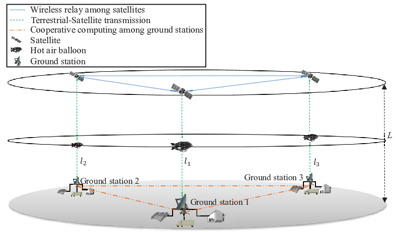

The considered system model is illustrated in Fig. 2, where S satellites constitute a low earth orbit (LEO) satellite network. The satellites provide service for S ground stations and each satellite has a dedicated ground station. Denote the number of satellites by S. We assume that the distance from all the satellites to the ground is the same, which is denoted by L. All satellites have the same orbital period given by
| (1) |
where =398,601.58 is the Kepler constant, and is the radius of the Earth. One hot air balloon is hovering above and serving its ground station to play the role of a dedicated relay between its ground station and the corresponding satellite. Considering the practical wireless and geographical environment, the distance from the hot air balloons to the ground stations generally differs with each other. We denote the distance from hot air balloon i () to its ground station by .
Due to the orbiting motion of LEO satellites, a hot air balloon can connect with a satellite periodically. The continuous serving time between the hot air balloon and the satellite in the is called a time window, which is determined by the minimal elevation angle from the hot air balloon to the satellite. An air balloon can exchange data with its satellite only within the corresponding time window.
Specifically, denote the minimal elevation angle from the hot air balloon i to its satellite by and the geocentric angle of the satellite i by . Generally, a hot air balloon at a lower height has a larger minimum elevation to the satellite due to the thicker atmosphere for the wireless transmission between the hot air balloon and the satellite. Then, it holds that [1]:
| (2) |
The time window of the satellite i denoted by , where , is given by
| (3) |
The ground stations are connected through a wired network to form a cooperative computing resource pool as shown in Fig. 2. This network has the computing ability to generate and execute the scheme of collaborative multi-resource allocation to be developed.
II-B LEO Satellites
The LEO satellite network considered in this work is shown in Fig. 2. We assume that, when the satellites circle the earth, they simultaneously arrive at the positions right above their corresponding hot air balloons. This is due to the identical orbital period for all satellites. As shown in Fig. 2, the time window for each satellite is equally divided into two parts by the straight line from the ground station to the hot air balloon.
Assume that the time windows of the S satellites in a LEO satellite network have . As shown in the lower part of Fig. 2, the time windows for satellites are symmetrical with respect to the vertical dashed line in the center, which denotes the instant when the satellites are right above their ground stations and hot air balloons. Within the time window of satellite , the following tasks should be completed: uplink transmission from the th hot air balloon to the th satellite, which takes a time duration of ; relay for the th satellite, which takes a time duration of ; and downlink transmission from the th satellite to the th hot air balloon, which takes a time duration of . As shown in the lower part of Fig. 2, with , we assume that .
As shown in the bottom part of Fig. 2, as there are S satellites and S time windows, the largest time window can be divided into S time segments. The time segments with sequence numbers are employed for traffic relay among satellites, where the value of can be determined by an iterative manner according to the system performance. Denote the th time segment by . Time segment , , is equally divided into two parts, which are symmetrical with respect to the central dashed straight line. In the sequel, the time length of time segment refers to the total length of these two parts, denoted as .
For the wireless channel between a satellite and a hot air balloon, as well as that between a hot air balloon and a ground station, we use the omnidirectional path loss model as in existing works [1, 21, 22, 23]. The path-loss (dB) for a link with distance l is denoted as:
| (4) |
where f is the system operating frequency and equals to 3 GHz in the S-band. The unit of the distance l is kilometer (km), and the unit of the frequency f is GHz in the above path loss model. Due to the line of sight (LOS) channels between the ground stations and the hot air balloons, and that between the hot air balloons and the satellites, we consider only path loss in the wireless channel power gain, , as follows.
| (5) |
For the LEO satellite network, we use the Starlink project launched by SpaceX as a reference [24]. LEO satellites use inter-satellite-links (ISLs) to form a satellite backbone network in a lattice grid manner [25]. For the inter-satellite links, we assume that Terahertz signal [26, 27, 28] or optical signal is employed. Each satellite is configured with multiple lasers to generate the signals at high frequency, and multiple antennas to transmit and receive the signals.
Signals working at high frequency are highly directional due to the narrow wave beam. As an instance, in Fig. 3, the transmitting-receiving antenna pair must be aligned. This feature can lead to the requirement of multiple schedules to relay data, because of the limited number of lasers and antenna pairs at each satellite. In Fig. 3, each satellite has a cache for storing the data to be transmitted to other satellites. We call a laser currently generating a high frequency signal as an active laser, and a laser that are currently not in use as an inactive laser. In the example shown in Fig. 3, let the maximum number of lasers be 2. Then, at least two schedules are needed to complete a full traffic relay cycle for this four satellites network. For example at satellite 1, the two lasers can generate the signals to be transmitted to satellite 2 and satellite 4, respectively. Thus, the data traffic heading to the satellite 3 will be transmitted in the next schedule.

II-C Traffic Relaying Among Satellites
Traffic relaying among satellites can be illustrated as shown in Fig. 3. Each data traffic stream is generated by a laser and sent by a transmitting antenna. The data traffic is relayed among satellites and received by the receiving antenna of the target satellite. In practice, one hop of the transmission can be built between two satellites with the distance less than or equal to a pre-determined threshold. If the distance from the source satellite to the target satellite is larger than the threshold, a relay satellite is required. For instance, in Fig. 3, satellite 3 sends its data to satellite 1 via path 3 consisting of path 3a and path 3b with satellite 2 as the relay. The inter-satellite data traffic is represented by a matrix , where is the amount of data from the source satellite i to the target satellite j. We have because satellite i does not need to send data to itself.
We assume that the number of schedules of the data is . Denote the average active number of lasers per satellite by , which is bounded by the maximum value of . Denote the power to launch a laser by . Denote the delay of aligning antennas before a scheduled transmission by . The basic energy consumption including circuit energy consumption, etc., for lasers of the satellites is
| (6) |
The velocity of electromagnetic signal propagation in space is m/s. Define the maximal distance among all paths of source-target satellites by . Then, the overhead involved in data transmission among satellites is . Prior to a scheduled transmission, overhead exists, which includes the alignment of antennas among satellites , and the data transmission time on paths of source-target satellites . The total overhead time, denoted by , is formulated as:
| (7) |
In eq. (7), for simplification, we assume that is the same for each satellite. Since we consider the upper bound of , can be treated as a constant in each schedule.
In Fig. 3, a pair of transmitting-receiving antennas can act as the relay for data transmission. The average traffic relay rate can be calculated by , where is the maximum relay time as shown in Fig. 2. Denote the static power consumption of one laser by W/bps, then, the static energy consumption of lasers is
| (8) |
Denote the dynamic power consumption of one laser by W/bps, and the capacity of the inter-satellite channels by bps. Then, the dynamic energy consumption of lasers is
| (9) |
In practice, may depend on the distance between satellites and the signal frequency. In this work, is assumed to be a constant for the considered TSN.
III Problem Formulation
In this section, we present the data process steps involved in the considered TSN and formulate a network energy efficiency maximization problem considering constraints on 3C resources.
III-A Data Transmission and Relay
A service period in the system consists of 6 steps and is described as follows.
- Step 1)
Accumulation of data at ground stations. Data is gathered and accumulated at the ground stations for time before each transmission, with given by
(10) where represents the number of circles the satellite orbiting over the Earth in between two transmissions, and is referred to as the serving period of satellites. We denote the maximum value of by so that is the maximum tolerable system delay at the ground stations. Denote the average data arrival rate by and the power consumption for caching data during the accumulation duration by W/bit. Then, the energy consumption for caching the data at the ith ground station is .
- Step 2)
Calculating the traffic scheduling and routing scheme. After the traffic accumulation, the computing servers of the ground stations cooperatively calculate the scheme of traffic scheduling and routing with a pre-determined algorithm. Denote the computing capacity of the cooperative computing pool at the ground stations by cycles/second (cps) and the computing demand of the data scheduling and routing in a network with S satellite by cycles, where is the average computing load for adding one satellite in the satellite relay network. The computing delay is give by
(11) In terms of the energy consumption of the computing resource, we denote the power consumption of the computing by W/cps. The corresponding energy consumption of computing is
(12) - Step 3)
Transmission of data traffic from ground stations to hot air balloons. Let denote the data transmission time from the th ground station to its serving hot air balloon with transmission power . Assume that the transmission bandwidth is , which is identical for all ground station to hot air balloon transmissions, and the power spectral density of the Gaussian white noise is W/Hz. By eq. (5), the wireless channel power gain is denoted by . Denote the antenna gain by , with , we can prove that
(13) The delay caused by the transmission is . In order to efficiently utilize the time window of for the inter-satellite relay and the rely between hot air balloons and satellites, we have following constraint,
(14) Constraint (14) means that the delay in step 2) plus step 3) should be within . Accordingly, the following three steps should be completed within the corresponding time windows.
- Step 4)
Data transmission from hot air balloons to satellites. The transmission time of the ith hot air balloon to the corresponding serving satellite is denoted by , which should be a portion of the time window of satellite . Denote the transmission power of the ith hot air balloon by . Denote the transmission bandwidth of a hot air balloon by , which is identical for all balloon to satellite transmissions. Denote the path loss based wireless channel power gain by . Then, with and , we can prove that
(15) The corresponding transmission delay is .
- Step 5)
Data relaying among satellites. After the data transmission from hot air balloons to satellites, the inter-satellite relaying is planned in multiple schedules for forwarding data to target satellites.
- Step 6)
Data transmission from satellites to hot air balloons. After the inter-satellite relaying, the data will be transmitted from satellites to hot air balloons, which takes a duration of length , and then forwarded to the target ground stations to complete a ground station to ground station data communication cycle. Denote the average data traffic arrival rate at satellite i, as a result of inter-satellite relaying, by . It holds that . The amount of the data received at satellite i in duration is then . Denote the transmission power of sending data from satellite i to its hot air balloon by . Denote the bandwidth by , which is identical for all satellite to balloon transmissions. The corresponding channel gain is . Then, with and , we have
(16) The propagation delay in this step is .
Next, the data collected at hot air balloons from satellites will be used for specific objectives such as store-and-forward for hot traffic or transmission to the ground stations for real-time traffic.
III-B Optimization Model

In this sub-section, we focus on formulating the system energy efficiency maximization problem. First, we illustrate the constraints of data transmission in the aforementioned 6 steps as in Fig. 4.The ordinate in Fig. 4 is the average power consumption for each step, and the abscissa is the time for each step. The propagation delay is denoted by for step 3, for step 4, and for step 6, respectively, as shown in Fig. 4. To avoid data overflow, in step 1 is the upper bound for each of the next steps. Since as shown in eq. (10), we have
| (17) |
and
| (18) |
There exists a trade-off between the delay and power consumption in each step, which will be discussed later.
| (19) |
| (20) |
Denote the total energy efficiency from Step 1 to Step 6 by . Considering the analysis above, can be formulated by eq. (19). In eq. (19), the denominator is the total amount of the data transmitted in one serving period. The overall energy consumption, used for caching, computing, wireless transmission (including the lasers), is formulated in the numerator of eq. (19). As there are many variables, we define a set of all variables in eq. (20).
Generally speaking, the energy consumption of antenna pairs depends on routing paths. The energy consumption of traffic scheduling for relay among satellites depends on the number of used lasers per satellite. In this work, we do not include the energy consumption for routing among the satellites in the free space and the antenna pairs, since this part of energy consumption is relatively small.
IV STMs Determination

As aforementioned, data relayed via inter-satellite communications constitutes a traffic matrix A. To solve the optimization problem (P1), we first study STMs determination based on different time window lengths of the satellites. The objective of the STMs determination is allocating the data traffic to different time segments. The relay scheduled for each time segment must happen within the time windows of the corresponding source and target satellites. Using the case shown in Fig. 3 for instance, each satellite caches the data to be relayed to the other three satellites. The different time window lengths of satellite determine the different available times for inter-satellite relaying, and the data for relaying indicated by the traffic matrix should be decomposed into multiple STMs, each for one specific time segment.
As shown in Fig. 5 (a), the time window contains , , and relay time . Without loss of generality, we assume that the length of the time window satisfies . We also assume that the maximum available time for inter-satellite relaying in Step 5 is within the relay time of the th satellite, i.e., , which is formulated as
| (21) |
where . By eq. (21), we have due to for . When and are determined, the value of can be found. As we have assumed, the length of the vth time segment is . Denote the length of the vth time segment by when . Then, we have , where is a constant determined by the length of time windows, and will be optimized later.
The data traffic matrix A can be decomposed into S STMs , each representing the data traffic to be relayed in the corresponding time segment. Since only the time segments with the sequence numbers are employed for traffic relay, are all-zero matrices, i.e., . The element of the ith row and the jth column of is denoted by , which represents the amount of data traffic transmitted from the ith satellite to the jth satellite during time segment . In the rest of this Section, we will solve the STMs generation problem.
IV-A Geometric-Water-Filling Algorithm


The objective of the STMs determination to different time segments with various length is to guarantee that the relay time is within the time windows of the corresponding source and destination satellites and to achieve data load balancing. Water-filling is well-known for deriving the optimal solutions for power allocation problems [19] as well as load balancing problems [20]. In the following, we introduce the geometric-water-filling (GWF) algorithm. More details can be found in [19, 20].
As shown in Fig. 7, we assume a water tank with uneven bottom steps. The width of the steps is denoted by vector W and height by vector H, representing the time segments width and already allocated data traffic density (i.e., data traffic per unit time), respectively. The total volume of water, , represents the total amount of data for distribution. The dashed horizontal line represents the formed water surface. The optimal distribution of these data amount is depicted by the water-filling algorithm. The solution returns a vector, X, the height of the distributed water above the steps, denoting the added traffic density for the corresponding time segment. In Fig. 7, the 4th step height is higher than the water surface, the solution of is then zero.
We can represent the geometric water-filling function as
| (22) |
The data amount scheduled for the th time segment is . The total data amount satisfies . The detailed solution approach can be referred in [19, 20]. Without loss of focus, we shall directly apply eq. (22) as a functional block to solve the STMs for satellites traffic relay.
IV-B Tapped Geometric-Water-Filling Based STMs Determination
In this subsection, we present the proposed algorithm for STMs determination. During the time window for the th satellite, we have a series of time segments, denoted as with width respectively. Data of the total traffic matrix A is allocated to STMs, , one for each time segment. We propose tapped geometric-water-filling (T-GWF) algorithm as described in Algorithm 1 to generate the STMs.
In the initialization stage of Algorithm 1, we set all STMs as all-zero matrices. The elements of the time segment width vector W are set to 0 for time segments to and the corresponding true width for time segments to . and represent the total data amount and the allocated amount, respectively.
In Line 1, a “For” loop is used, running from the th time segment to the th time segment. Before the th time segment, we start from time segment , where the th row and the th column of the traffic matrix A is stored in and respectively in Lines 3 and 4. The total amount of data for the allocation in this round is denoted by as shown in Line 5.
In Line 11, the GWF algorithm is applied to conduct data traffic allocation. The notation denotes a vector consisting of the th element to the th element of vector W. We design a mechanism recursively updating the STMs through GWF operation. We model that the time segments are separated by a series of taps, shown as the vertical arrowed dashed-lines in Fig.7. Starting from , when GWF works for the th segment, and all the taps are in their closed positions. Then when , the right most tap is removed and the data traffic can be distributed in time segments to . For all the time segments involved in the traffic allocation, the newly allocated traffic is frozen and added on the top of the current step height to update the step height for the next round GWF calculation. The taps are lifted one by one from right to left, until the last tap for the time segment . We refer to the proposed Algorithm 1 as T-GWF algorithm for this nature.
In Line 12 of Algorithm 1, the step height is updated. In the following “For” loop, Before the th time segment, the STMs are updated with the scaled th row and th column of the traffic matrix A. The scale factor is the ratio of the allocated traffic for a specific participating time segment to the total allocated traffic.
The last step of the outer “For” loop is to allocate data when , i.e., for the time segment . The data traffic for allocation is a sub-matrix of A, consisting of its first row to the th row, and from the first column to the th column, as listed in Line 9. In the inner “For” loop, the STMs are updated in Line 20. Different with Lines 17 and 18, where each update is carried for a row and a column respectively, each update is adding a scaled sub-matrix.
The proposed T-GWF have two great advantages. The first one is to distribute the data traffic among participating time segments to guarantee the relay being in the time windows of the involved source and destination satellites and to achieve load balance. GWF can efficiently solve this problem. The second advantage is the structure of the water-filling solution facilitating the STMs update.
Water-filling structured solution by T-GWF also reveals that the obtained water level for each time segment represents the corresponding data rate, or equivalently, data traffic density. For time segment to , the water level is non-decreasing. This reflects that satellites relaying data traffic is not uniform across the time segments, but tends to be more intense towards the central point of the time windows. This is reasonable since the closer to the central point, the more data traffic uploaded from the air balloons is available.
V Configuration Matrices Generation
After the STMs determination, the data traffic represented by the STM , with the dimension of , is relayed in the time segment of . Define a set of configuration matrices with the dimension of so that each row and each column for a configuration matrix has at most one, respectively. The rest of the elements for the configuration matrix are all zeroes. The time for transmitting one bit of data, i.e., the inverse of the data transmission rate, is seconds, where . Assume that when , each configuration matrix has a coefficient , which denotes the number of to relay the data traffic in the configuration matrix. Then, for a general form when , each configuration matrix generated from the STM has a coefficient . For simplicity, we assume that is the same for each configuration matrix.
To determine the required number of active lasers per satellite, i.e., , we assume that configuration matrices are firstly generated for . If the configuration matrices are implemented by satellites with one laser per satellite, the delay is by . Then, when lasers are configured for each satellite, the satellites can simultaneously relay data traffic according to configuration matrices, which can be formulated as
| (23) |
In practice, should be small to reduce the power consumption and the hardware cost of the satellites. We can have
| (24) |
From eq. (24), a smaller leads to a larger . This is because that a smaller increases ineffective occupation time of the transmitting-receiving antenna pairs after the data traffic has been relayed in a configuration matrix. On the other hand, should be no less than to cover all the elements in .
When , we denote the average maximum summation of the elements in either a row or a column of by . Then, when , the average maximum summation of the elements in either a row or a column of is . We propose Theorem 1 as follows.
Theorem 1 Define as follows, with a unit of bits:
| (25) |
Then, can be covered by at most configuration matrices. The corresponding time delay for transmitting bits of data is .
Proof: See Appendix A.
Considering Theorem 1, in eq. (24), we have
| (26) |
This guarantees the feasibility of the configuration matrices generation.
By eqs. (24) and (25), we can further derive that
| (27) |
In practice, can be rounded up to an integer, i.e., .
| (P2) |
| (P3) |
To maximize the energy efficiency of the active lasers, we define the average number of active lasers as
| (28) |
By eq. (6), can be re-formulated by
| (29) |
By eqs. (8) and (9), the static energy consumption and dynamic energy consumption can be formulated in eqs. (30) and (31), respectively, as follows:
| (30) |
| (31) |

In Fig. 8, using a LEO satellite network with 4 satellites, we demonstrate an example of the configuration matrices generation for a specific time segment v with the sub-traffic-matrix . We assume that bps, s, s, and . Then, s/bit, i.e., it takes seconds for relaying 1 bit of data among satellites. By Theorem 1, we can find that bits. This suggests that the transmission delay is s for a schedule. Furthermore, can be calculated by eq. (27) and rounded up to an integer, which gives .
is decomposed into configuration matrices, each of which has a coefficient . The specific elements in a configuration matrix are determined by the traffic scheduling, which in turn depends on the data traffic routing among satellites and the number of transmitting-receiving antenna pairs, etc. We show an example of traffic scheduling for the configuration matrices in Fig. 8. Since , each satellite can transmit at most one data stream at any given time. Thus, it takes 7 schedules for completing the relay among satellites. For the third configuration matrix, satellite 1 transmits to satellite 4, while satellite 2 transmits to satellite 3, using satellite 1 and satellite 4 as relays. In our future work, we will discuss the data traffic scheduling in each configuration matrix and the corresponding routing schemes for relay among satellites.
VI Collaborative Multi-Resource Allocation
In this section, we present the approximation and transformation to solve the original optimization problem of (P1).
VI-A Optimization with Taylor Approximation for Collaborative Multi-Resource Allocation
By the expansion of the problem (P1) with eqs. 10, 11, 21, 13, 15, 16, 12, 29, 30 and 31, as well as the constraints of and , optimization problem (P1) can be transformed into problem (P2).
Let . For a variable x, by Taylor series, we have , which leads to
| (32) |
Then, optimization problem (P2) can be further transformed into problem (P3), which is a standard geometric programming problem solvable by CVX [29].
In (P3), is a positive integer that denotes the maximum number of terms used in the Taylor series. We propose Algorithm 2 to solve problem (P3). In Algorithm 2, is determined in an iterative manner until the values of all optimization variables converge. It is difficult to determine the optimal value of , especially when the number of time segments is large. In Algorithm 2, the value of is determined heuristically, and its value stops updating when the system energy efficiency does not increase further as increases.
VII Numerical Results
VII-A Simulations
center \onelinecaptionsfalse
Simulation Parameters
| Parameter | Value | Parameter | Value | Parameter | Value | Parameter | Value |
|---|---|---|---|---|---|---|---|
| 10 | S | 5 | L | 550 km | (15 dB) | ||
| V | m/s | cycles/bit | cycles/second | bps | |||
| Hz | Hz | Hz | W/bit | ||||
| W/cps | W/bps | W/bps | W/laser | ||||
| km | 1 second | 20 | 50 |


Table I gives the general simulation parameters. The noise temperature is assumed to be 260 K. We consider satellites deployed at the height of 550 km above the Earth, same as the setting used in the Starlink LEO network. This leads to a maximum routing distance being equal to half of the orbit circumference, i.e., km. Then, the maximum delay of data routing among satellites is s.
The hot air balloon with the minimum height is deployed at km, and the maximum height at km above the earth. The height of the remaining hot air balloons is evenly distributed between and . The hot air balloon at lower height generally has a larger minimum elevation to the satellite. We set the minimum elevation, for the hot air balloon at the maximum and the minimum height to the Earth, to and , respectively. The minimum elevation of the other hot air balloons is evenly distributed between and . The traffic matrix A is randomly generated, where the diagonal elements are 0, and the other entries of A are random and uniformly distributed over [0, ] bits. Unless otherwise specified, we assume that bits.
Since the system model that we consider is new, there is no existing algorithm that considers the same network model and scenario for comparison. To evaluate the performance of our proposed scheme, we name the scheme using both Algorithm 1 and Algorithm 2 as scheme 1. Let scheme 2 be the semi-fixed method using Algorithm 1 and Algorithm 2 with and . Let scheme 3 be the semi-fixed method using Algorithm 1 and Algorithm 2 with and . Then, the performance of scheme 1 is compared with those of scheme 2 and scheme 3.
In Fig. 9, the performance of the three schemes versus the maximum value of , i.e., , is illustrated. In Fig. 9(a), as increases, the energy efficiency of the schemes 1 and 2 firstly increases due to the increased throughput and relatively small energy consumption. As further increases, the energy efficiency gradually saturates because of the ever-increasing energy consumption. Scheme 3 has a fixed energy efficiency performance because its remains 1, then the energy efficiency is independent on . Based on the figure, our proposed scheme 1 outperforms the other schemes in terms of energy efficiency. The gap is much smaller between the performance of schemes 1 and 2 than between the performance of schemes 1 and 3. This suggests that more frequent transmission in a terrestrial-satellite network cannot guarantee a larger energy efficiency, because the large power consumption only supports a limited amount of data traffic corresponding to a relatively small . In Fig. 9(b), the required increases for both schemes 1 and 2. This is because when the amount of data is relatively small, an increasing leads to a larger amount of data traffic, which enables higher energy efficiency. From Fig. 9(c), we can verify that the required increases for schemes 1 and 2 to meet the relay requirement among satellites due to the increasing amount of data traffic. As further increases, remains constant for schemes 1 and 2, because the amount of data traffic remains. In Fig. 9(d), for scheme 1 gradually decreases, because the increasing amount of data traffic requires a longer time interval to transmit between satellites and hot air balloons.
In Fig. 10, the performance of the three schemes versus the number of satellites S is illustrated. In Fig. 10(a), as S increases, the energy efficiency performance of schemes 1 and 2 monotonously decreases. This is because a larger S results in a larger power consumption dominating the performance of energy efficiency in wireless transmission and the lasers for relay. For scheme 3, as S increases, the energy efficiency firstly increases because the increasing amount of data traffic brought by the increased satellites. As S further increases, the energy efficiency of the schemes 1 and 3 gradually merges. This is because, as S increases, the optimal is 1 to decrease the energy consumption of lasers and wireless transmission. This can be verified in Fig. 10(b), in which the required approaches 1 for all the schemes as S increases. In Fig. 10(b), the for scheme 1 is larger than that of scheme 2 when . This suggests that scheme 1 can support a larger amount of data traffic due to the optimal resource allocation. In Fig. 10(c), as S further increases, also increases due to the increasing amount of data traffic. The optimal for scheme 2 is larger than those of schemes 1 and 3. This is caused by the smaller for scheme 2, which can be verified in Fig. 10(d). In Fig. 10(d), as S increases, the required for both the scheme 1 and scheme 3 gradually increases, because the increased power consumption by lasers for relay among satellites. As S further increases, the required of schemes 1 and 3 gradually remains and merges. This is because that approaches 1 for both schemes. Then, the performance of scheme 1 becomes the same with that of scheme 3.
In Fig. 11, we illustrate the energy efficiency versus , the maximum amount of data to relay between arbitrary two satellites, and , the maximum minimal elevation angle, respectively. In Fig. 11(a), as increases, the energy efficiency firstly increases for all the schemes. This is because a larger can increase the data traffic amount to improve the energy efficiency. As further increases, the energy efficiency arrives the peak and then gradually falls for all three schemes, because the high power consumption used for communications. In Fig. 11(b), as increases, the energy efficiency of schemes 1 and 2 monotonously decreases. This is because a larger leads to a smaller time windows between hot air balloons and satellites. Accordingly, a shorter relay time among satellites causes higher power consumption of relay by lasers and reduced energy efficiency. For the scheme 3, the energy efficiency remains constant, because a smaller will not cause the higher power consumption by lasers when is not very large.

VII-B Discussions
We have studied a relatively complex system model in this work, including: 1) different hovering heights of the hot air balloons with different minimum elevation angle from hot air balloons to the satellites; 2) the caching, computing, and communication power consumption in this integrated system; 3) different lengths of time windows and the corresponding STMs determination for relay among satellites; 4) the configuration matrix generation to form multiple configuration matrices corresponding to the schedules; 5) an integrated optimization of the variables to maximize the overall system energy efficiency.
Two directions can be considered for future works, which can advance the research in terrestrial-satellite networks.
Firstly, joint traffic scheduling and routing scheme is of interest. As illustrated in Fig. 8, the joint traffic scheduling and routing can be considered to determine the elements in a specific configuration matrix. The elements in configuration matrices will determine the number of the active lasers and affect the number of transmitting-receiving antenna pairs. Additionally, the routing scheme of traffic relay among satellites also effects the performance of the total routing distance and the number of transmitting-receiving antenna pairs in use at each satellite.
Secondly, in this work, we assume that the time windows are overlapping and symmetrical with respective to a central line, as shown in the lower part of Fig. 2. The central line represents the assumption that the satellites will simultaneously arrive right above their corresponding hot air balloons. For a large satellite network, such assumption might not be practical. Instead, as shown on the left-hand side of Fig. 12, the starting point of the time windows for the satellites may differ with each other, leading to asymmetric time windows as shown on the right-hand side of Fig. 12. In the figure, when the satellite k is right above its hot air balloon, the time window of satellite j just starts, and the time window of satellite i is yet to start. In this scenario, the STM determination needs further investigation.
Lastly, applications, such as content provision [30], can be studied based on our proposed framework for TSN.

VIII Conclusion
In this work, we studied the energy efficiency performance of TSN while jointly considering the caching, computing, and communication resources. We considered a practical scenario, in which different hot air balloons can be deployed at different heights with different minimum elevation angles. To effectively utilize the time windows between satellites and hot air balloons, we investigated STM determination according to the length of the time windows, through which we achieved balanced load for relaying and guaranteed that relaying happens within the time windows of the corresponding source and target satellites. We also proposed a configuration matrix generation algorithm to obtain the optimal number of lasers per satellite under the constraint of the available relay time. Then, we solved the collaborative multi-resource allocation problem to optimize the transmission power, the serving period of satellites, and the required number of lasers per satellites at the relays for the maximum system energy efficiency. Simulation results verified the effectiveness of our proposed scheme, and potential future directions were discussed.
Appendix A Proof of Theorem 1
Proof: since the maximum line summation of is , i.e., and . Define and , Let
| (33) |
where
| (34) |
and .
Hence, the maximum line summation of is . According to graph theory [31], the corresponding bipartite graph of Q has the maximum endpoint degree . Then, Q can be decomposed into configuration matrices with the coefficient of 1 for each. Moreover, by eq. (33), we have . This suggests that R can be covered by at most S configuration matrices with the coefficient of for each. Then, can be covered by at most configuration matrices, each of which the coefficient of .
References
- [1] S. Fu, J. Gao, and L. Zhao, “Integrated resource management for terrestrial-satellite systems,” IEEE Transactions on Vehicular Technology, vol. 69, no. 3, pp. 3256–3266, 2020.
- [2] C. Qiu, H. Yao, R. Yu, F. Xu, and C. Zhao, “Deep Q-learning aided networking, caching, and computing resources allocation in software-defined satellite-terrestrial networks,” IEEE Transactions on Vehicular Technology, vol. 68, no. 6, pp. 5871–5883, 2019.
- [3] P. V. R. Ferreira, R. Paffenroth, A. M. Wyglinski, T. M. Hackett, S. G. Bilen, R. C. Reinhart, and D. J. Mortensen, “Reinforcement learning for satellite communications: From LEO to deep space operations,” IEEE Communications Magazine, vol. 57, no. 5, pp. 70–75, 2019.
- [4] Y. Liang, J. Tan, H. Jia, J. Zhang, and L. Zhao, “Realizing intelligent spectrum management for integrated satellite and terrestrial networks,” (invited), Journal of Communications and Information Networks, vol. 6, no. 1, pp. 32–43, 2021.
- [5] Z. Chen, X. Ma, B. Zhang, Y. Zhang, Z. Niu, N. Kuang, W. Chen, L. Li, and S. Li, “A survey on Terahertz communications,” China Communications, vol. 16, no. 2, pp. 1–35, 2019.
- [6] Y. L. L. Zhang and D. Niyato., “6G visions: mobile ultra-broadband, super internet-of-things, and artificial intelligence,” China Communications, vol. 16, no. 8, pp. 1–14, 2019.
- [7] J. Gao, L. Zhao, and X. Shen, “The study of dynamic caching via state transition field - the case of time-invariant popularity,” IEEE Transactions on Wireless Communications, vol. 18, no. 12, pp. 5924–5937, 2019.
- [8] S. Fu, J. Wu, H. Wen, Y. Cai, and B. Wu, “Software defined wireline-wireless cross-networks: Framework, challenges, and prospects,” IEEE Communications Magazine, vol. 56, no. 8, pp. 145–151, 2018.
- [9] B. Feng, G. Li, G. Li, Y. Zhang, H. Zhou, and S. Yu, “Enabling efficient service function chains at terrestrial-satellite hybrid cloud networks,” IEEE Network, vol. 33, no. 6, pp. 94–99, 2019.
- [10] C. Dai, G. Zheng, and Q. Chen, “Satellite constellation design with multi-objective genetic algorithm for regional terrestrial satellite network,” China Communications, vol. 15, no. 8, pp. 1–10, 2018.
- [11] B. Di, L. Song, Y. Li, and H. V. Poor, “Ultra-dense leo: Integration of satellite access networks into 5g and beyond,” IEEE Wireless Communications, vol. 26, no. 2, pp. 62–69, 2019.
- [12] N. Zhang, S. Zhang, P. Yang, O. Alhussein, W. Zhuang, and X. S. Shen, “Software defined space-air-ground integrated vehicular networks: challenges and solutions,” IEEE Communications Magazine, vol. 55, no. 7, pp. 101–109, 2017.
- [13] J. Wang, C. Jiang, Z. Wei, C. Pan, H. Zhang, and Y. Ren, “Joint UAV hovering altitude and power control for space-air-ground IoT networks,” IEEE Internet of Things Journal, vol. 6, no. 2, pp. 1741–1753, 2019.
- [14] S. Fu, Y. Tang, N. Zhang, L. Zhao, S. Wu, and X. Jian, “Joint unmanned aerial vehicle (UAV) deployment and power control for internet of things networks,” IEEE Transactions on Vehicular Technology, vol. 69, no. 4, pp. 4367–4378, 2020.
- [15] M. Li, N. Cheng, J. Gao, Y. Wang, L. Zhao, and X. S. Shen, “Energy-efficient UAV-assisted mobile edge computing: Resource allocation and trajectory optimization,” IEEE Transactions on Vehicular Technology, vol. 69, no. 3, pp. 3424–3438, 2020.
- [16] X. Sun and S. Cao, “A routing and wavelength assignment algorithm based on two types of LEO constellations in optical satellite networks,” IEEE Journal of Lightwave Technology, vol. 38, no. 8, pp. 2106–2113, 2020.
- [17] B. Wu, S. Fu, X. Jiang, and H. Wen, “Joint scheduling and routing for QoS guaranteed packet transmission in energy efficient reconfigurable WDM mesh networks,” IEEE Journal on Selected Areas in Communications, vol. 32, no. 8, pp. 1533–1541, 2014.
- [18] P. K. Upadhyay and P. K. Sharma, “Max-Max user-relay selection scheme in multiuser and multirelay hybrid satellite-terrestrial relay systems,” IEEE Communications Letters, vol. 20, no. 2, pp. 268–271, 2016.
- [19] P. He, L. Zhao, S. Zhou, and Z. Niu, “Water-filling: A geometric approach and its application to solve generalized radio resource allocation problems,” IEEE Transactions on Wireless Communications, vol. 12, no. 7, pp. 3637–3647, 2013.
- [20] P. He, M. Li, L. Zhao, B. Venkatesh, and H. Li, “Water-filling exact solutions for load balancing of smart power grid systems,” IEEE Transactions on Wireless Communications, vol. 9, no. 2, pp. 1397–140, 2018.
- [21] X. Zhu, C. Jiang, L. Kuang, N. Ge, and J. Lu, “Non-orthogonal multiple access based integrated terrestrial-satellite networks,” IEEE Journal on Selected Areas in Communications, vol. 35, no. 10, pp. 2253–2267, 2017.
- [22] B. Deng, C. Jiang, J. Yan, N. Ge, S. Guo, and S. Zhao, “Joint multigroup precoding and resource allocation in integrated terrestrial-satellite networks,” IEEE Transactions on Vehicular Technology, vol. 68, no. 8, pp. 8075–8090, 2019.
- [23] Y. Zhang, L. Yin, C. Jiang, and Y. Qian, “Joint beamforming design and resource allocation for terrestrial-satellite cooperation system,” IEEE Transactions on Communications, vol. 68, no. 2, pp. 778–791, 2020.
- [24] “SpaceX gets OK to re-space Starlink orbits,” in SpaceNews.com, December 2019.
- [25] J. Hu, L. Cai, C. Zhao, and J. Pan, “Directed percolation routing for ultra-reliable and low-latency services in low earth orbit (LEO) satellite networks,” in Proceedings of IEEE Vehicular Technology Conference Workshop (VTC Fall Workshop), 2020, pp. 1–6.
- [26] X. Wang, P. Wang, M. Ding, Z. Lin, F. Lin, B. Vucetic, and L. Hanzo, “Performance analysis of TeraHertz unmanned aerial vehicular networks,” IEEE Transactions on Vehicular Technology, vol. PP, no. 99, pp. 1–6, 2020.
- [27] K. Tekbiyik, A. R. Ekti, G. K. Kurt, A. Gorcin, and H. Yanikomeroglu, “A holistic investigation of Terahertz propagation and channel modeling toward vertical heterogeneous networks,” IEEE Communications Magazine, vol. 58, no. 11, pp. 14–20, 2020.
- [28] H. Yuan, N. Yang, K. Yang, C. Han, and J. An, “Enabling massive connections using hybrid beamforming in Terahertz micro-scale networks,” in Proceedings of IEEE Wireless Communications and Networking Conference (WCNC), 2020, pp. 1–7.
- [29] C. M., Geometric programming for communication systems. Hanover: Now Publishers, 2005.
- [30] S. Zhang, J. Li, H. Luo, J. Gao, L. Zhao, and X. S. Shen, “Low-latency and fresh content provision in information-centric vehicular networks,” IEEE Transactions on Mobile Computing, pp. 1–1, dOI:10.1109/TMC.2020.3025201, to appear.
- [31] R. Diestel, Graph Theory (2nd ed). New York: Springer-Verlag, 2000.