跳到论文正文
W Papers独立论文阅读器 arXiv:2105.01232 论文正文 计算阅读时间 · 0%
引用这篇论文根据当前论文元数据生成,正式投稿前建议核对。


License: CC BY 4.0
arXiv:2105.01232v1 [math.PR] 04 May 2021

Integration and stochastic integration
in Gaussian multiplicative chaos

Isao Sauzedde Address: Isao Sauzedde – LPSM, Sorbonne Université, Paris Email address: isao.sauzedde@lpsm.paris
Abstract.

We show that for γ<4/3\gamma<\sqrt{4/3}, it is possible to define the Lévy area of a planar Brownian motion with the Liouville measure of intermittency parameter γ\gamma as the underlying area measure. We also consider the case of smoother curves, and study some properties of the integration map thus defined.

Key words and phrases:
Green’s formula, Planar Brownian motion, Lévy area, Liouville measure

Introduction

In a previous paper [13], we showed a Green formula for α\alpha-Hölder continuous planar curves (with α>12\alpha>\frac{1}{2}) and for the planar Brownian motion. It allows us to compute the Young or Stratonovich integral of a smooth differential 11-form η\eta along the curve XX as the surface integral of the winding function θX\theta_{X} against the 22-form d​η{\rm d}\eta. In the Brownian case, the surface integral has be interpreted through a principal value method.

In the present paper, we look at the same integrals but with the smooth 22-form d​η{\rm d}\eta replaced with a random measure, the Liouville measure of parameter γ\gamma. For a planar Brownian motion independent of the Liouville measure, we show that, for γ<4/3\gamma<\sqrt{4/3}, the principal value is still well defined and lies in L2L^{2} of the product probability space. We also prove continuity, Hölder continuity, and additivity (‘Chen’s relation’) of the integral thus defined. For the case of α\alpha-Hölder continuous curves, we show similar results, provided γ\gamma is small enough and α\alpha is large enough.

For a continuous curve X:[s,t]→ℝ2X:[s,t]\to\mathbb{R}^{2}, we denote by X¯\bar{X} the concatenation of XX with the straight line segment from XtX_{t} to XsX_{s}. This is an oriented loop, and for all point z∈ℝ2∖Range⁡(X¯)z\in\mathbb{R}^{2}\setminus\Range(\bar{X}), we denote by θX​(z)∈ℤ\theta_{X}(z)\in\mathbb{Z} the winding of this oriented loop X¯\bar{X} around the point zz. Provided XX is a smooth curve, Green’s theorem is easily seen to implies that for all smooth 11-form η\eta,

(1) ∫X¯η=∫ℝ2θX​𝑑η.\int_{\bar{X}}\eta=\int_{\mathbb{R}^{2}}\theta_{X}\;{\rm d}\eta.

In [13], we showed that this equality extends to all α\alpha-Hölder continuous curves XX with α>12\alpha>\frac{1}{2}. For this, the left-hand side must be interpreted as a Young integral. We further proved that a similar equality also holds for the Brownian motion (in the particular case η=x​d​y\eta=x\;{\rm d}y, but we can deduce the general case with a few extra work), provided we interpret the left-hand side as a Stratonovich integral and the right-hand side as a kind of principal value. To be more specific, and using superscripts to indicates the coordinates in ℝ2\mathbb{R}^{2}, and denoting the Lebesgue measure by λ\lambda, one has almost surely

∫01X1∘d​X2+∫01((1−r)​X1+r​X0)1​(X0−X1)2​𝑑r\displaystyle\int_{0}^{1}X^{1}\circ{\rm d}X^{2}+\int_{0}^{1}((1-r)X_{1}+rX_{0})^{1}(X_{0}-X_{1})^{2}\;{\rm d}r =limK→+∞∫ℝ2𝟙{|θX(z)|≤K}θX(z)dλ(z)\displaystyle=\lim_{K\to+\infty}\int_{\mathbb{R}^{2}}\mathbbm{1}_{\{|\theta_{X}(z)|\leq K\}}\,\theta_{X}(z)\;{\rm d}\lambda(z)
(2) =limK→+∞∫ℝ2max⁡(−K,min⁡(θX​(z),K))​𝑑λ​(z).\displaystyle\hskip-42.67912pt=\lim_{K\to+\infty}\int_{\mathbb{R}^{2}}\max(-K,\min(\theta_{X}(z),K))\;{\rm d}\lambda(z).

The goal of this paper is to study the right-hand sides of (1) and (2), but with d​η\!\;{\rm d}\eta (resp. d​z{\rm d}z) replaced with a Gaussian multiplicative chaos, that we denote by 𝖬\mathsf{M}.

In this paper, 𝖬\mathsf{M} will be a random measure heuristically described by the formula

(3) ∀A∈ℬ⁡(ℝ2),𝖬⁡(A)=∫Aexp⁡(γ​Φz−γ22​𝔼​[Φz2])​𝑑λ​(z),\forall A\in\mathcal{B}(\mathbb{R}^{2}),\qquad\mathsf{M}(A)=\int_{A}\exp\big(\gamma\Phi_{z}-\tfrac{\gamma^{2}}{2}\mathbb{E}[\Phi_{z}^{2}]\big)\;{\rm d}\lambda(z),

where Φ\Phi is a centered Gaussian field, and γ∈[0,2)\gamma\in[0,2). It is assumed that the covariance kernel K:ℝ2×ℝ2→ℝ+∪{∞}K:\mathbb{R}^{2}\times\mathbb{R}^{2}\to\mathbb{R}_{+}\cup\{\infty\} of Φ\Phi takes the form

K⁡(z,w)=log+⁡(|z−w|−1)+g⁡(z,w),K(z,w)=\log_{+}(|z-w|^{-1})+g(z,w),

where log+\log_{+} is the positive part of the logarithm and g:ℝ2×ℝ2→ℝg:\mathbb{R}^{2}\times\mathbb{R}^{2}\to\mathbb{R} is a bounded and 𝒞2\mathcal{C}^{2}-function with bounded derivatives up to order 22. The kernel KK is well defined, as well as the random field Φ\Phi, even though the logarithmic divergence of KK makes Φ\Phi a random distribution rather than a random function. However, precisely because Φ\Phi is a random distribution, (3) does not make sense, and the construction of 𝖬\mathsf{M} cannot rely on this formula. The first construction of a random measure that is a reasonable candidate to be a mathematical incarnation of (3) was given using the theory of multiplicative chaos by Kahane [9]. For an introduction to Gaussian multiplicative chaos, see also [11] and [2]. In general, the larger γ\gamma, the more irregular the measure. Most of the time in this paper, we will be working in the case where γ<2\gamma<\sqrt{2}. We will thus be in the so-called ‘L2L^{2}-phase’, in which it is relatively easy to define and to study 𝖬\mathsf{M}, using martingale methods and Hilbertian techniques.

For the reader more familiar with multiplicative chaos, let us mention that the condition g∈𝒞2g\in\mathcal{C}^{2} is not necessary to define the measure 𝖬\mathsf{M}, nor to study the integral along Hölder paths, but it is a practical one when we look at the integral along Brownian paths.

We will denote by (Ω𝖬,ℱ𝖬,ℙ𝖬)(\Omega^{\mathsf{M}},\mathcal{F}^{\mathsf{M}},\mathbb{P}^{\mathsf{M}}) the probability space on which 𝖬\mathsf{M} is defined. We also let (ΩX,ℱX,ℙX)(\Omega^{X},\mathcal{F}^{X},\mathbb{P}^{X}) be a second probability space, on which a planar Brownian motion X=(Xt)t∈[0,1]X=(X_{t})_{t\in[0,1]} is defined. Finally, we denote by (Ω,ℱ,ℙ)(\Omega,\mathcal{F},\mathbb{P}) the product probability space.

The first part of this paper (Sections 1 to 5) is dedicated to the proof of the following result. Let us emphasize that we stop the Brownian motion at time 11.

Theorem 1.

Assume γ<4/3\gamma<\sqrt{4/3}. Then, ℙ\mathbb{P}-almost surely, the integral

∫ℝ2max⁡(−K,min⁡(θX​(z),K))​𝑑𝖬​(z)\int_{\mathbb{R}^{2}}\max(-K,\min(\theta_{X}(z),K))\;{\rm d}\mathsf{M}(z)

admits a limit 𝔸X\mathbb{A}^{X} as K→+∞K\to+\infty.

Moreover, for all p∈[2,4γ2)p\in[2,\frac{4}{\gamma^{2}}), this limit lies in Lp​(ΩX,L2​(Ω𝖬))L^{p}(\Omega^{X},L^{2}(\Omega^{\mathsf{M}})).11 1 The reader may find surprising, as we do, that the integrability with respect to ℙX\mathbb{P}^{X} depends on γ\gamma, and not the integrability with respect to ℙ𝖬\mathbb{P}^{\mathsf{M}}. However, the result as it is written is what we mean.

For (s,t)∈Δ={(s,t)∈[0,1]2:s≤t}(s,t)\in\Delta=\{(s,t)\in[0,1]^{2}:s\leq t\}, we denote by 𝔸s,tX\mathbb{A}_{s,t}^{X} the almost surely defined limit,

(4) 𝔸s,tX=limK→+∞∫ℝ2max(−K,min(θX|[s,t](z),K))d𝖬(z).\mathbb{A}_{s,t}^{X}=\lim_{K\to+\infty}\int_{\mathbb{R}^{2}}\max(-K,\min(\theta_{X_{|[s,t]}}(z),K))\;{\rm d}\mathsf{M}(z).

The second part of the paper (Section 6 to 9) is devoted to the study of the map (s,t)↦𝔸s,tX(s,t)\mapsto\mathbb{A}_{s,t}^{X}, and also, for a curve YY deterministic and more regular than a Brownian motion, of the map 𝔸s,tY\mathbb{A}_{s,t}^{Y} given by

(5) 𝔸s,tY=∫ℝ2θY|[s,t]d𝖬.\mathbb{A}_{s,t}^{Y}=\int_{\mathbb{R}^{2}}\theta_{Y_{|[s,t]}}\;{\rm d}\mathsf{M}.

For a function 𝔸:Δ→ℝ\mathbb{A}:\Delta\to\mathbb{R} to deserve the name of ‘algebraic 𝖬\mathsf{M}-area enclosed by the curve ZZ’, it should satisfy a relation that we will call a Chen relation. To write this relation, let us denote, for all s≤u≤ts\leq u\leq t, by Ts,u,tT_{s,u,t} the triangle with vertices ZsZ_{s}, ZuZ_{u} and ZtZ_{t}. Let us also set εs,u,t=1\varepsilon_{s,u,t}=1 if ZsZ_{s}, ZuZ_{u} and ZtZ_{t} are found in this cyclic order along the positively oriented boundary of Ts,u,tT_{s,u,t}, and εs,u,t=−1\varepsilon_{s,u,t}=-1 otherwise. We say that 𝔸\mathbb{A} satisfies the Chen relation (relative to ZZ) if for all s≤u≤ts\leq u\leq t,

𝔸s,t=𝔸s,u+𝔸u,t+εs,u,t​𝖬​(Ts,u,t).{\mathbb{A}}_{s,t}={\mathbb{A}}_{s,u}+{\mathbb{A}}_{u,t}+\varepsilon_{s,u,t}\mathsf{M}(T_{s,u,t}).

In a nutshell, the results of this second part can be summarized as follows (some additional properties are given below).

Theorem 2.

Let γ<2​(2−1)\gamma<2(\sqrt{2}-1), and Z:[0,1]→ℝ2Z:[0,1]\to\mathbb{R}^{2} be either a planar Brownian motion or an α\alpha-Hölder continuous function with α>(2​(1−γ24))−1\alpha>\big(2(1-\frac{\gamma^{2}}{4})\big)^{-1}. Then, for all (s,t)∈Δ(s,t)\in\Delta, almost surely, 𝔸s,tZ\mathbb{A}_{s,t}^{Z} is well-defined. It admits a modification which is continuous, Hölder continuous, and satisfies the Chen relation.

Let us also say that 𝔸\mathbb{A} is β\beta-regular if there exists a constant CC such that for all (s,t)∈Δ(s,t)\in\Delta,

(6) 𝔸s,t≤C​(t−s)β.\mathbb{A}_{s,t}\leq C(t-s)^{\beta}.

From now on, we set ν=2​(1−γ24)\nu=2(1-\frac{\gamma^{2}}{4}).33 3 This number ν\nu is the Hausdorff dimension of a Borel set of full 𝖬\mathsf{M}-measure. However, the reason why it matters to us is that it is equal to ξ⁡(q)q|q=2=ξ⁡(2)2\frac{\xi(q)}{q}|_{q=2}=\frac{\xi(2)}{2}, where ξ\xi the so-called structure exponent of 𝖬\mathsf{M}. This exponent is defined by the fact that for r>0r>0, the expectation of 𝖬​(B⁡(0,r))q\mathsf{M}(B(0,r))^{q} is of the order of rξ⁡(q)r^{\xi(q)}.

Theorem 3.

Let γ<4/3\gamma<\sqrt{4/3}. Then, (𝔸s,tX)(s,t)∈Δ(\mathbb{A}_{s,t}^{X})_{(s,t)\in\Delta} admits a modification which satisfies the Chen relation.

Let γ<2​(2−1)≃0.81\gamma<2(\sqrt{2}-1)\simeq 0.81. Then, (𝔸s,tX)(s,t)∈Δ(\mathbb{A}_{s,t}^{X})_{(s,t)\in\Delta} admits a modification which satisfies the Chen relation, is β\beta-regular for all β<min⁡(12−γ24,1+γ24−2​γ)\beta<\min(\frac{1}{2}-\frac{\gamma^{2}}{4},1+\frac{\gamma^{2}}{4}-\sqrt{2}\gamma), and β\beta-Hölder continuous for all β<12​(1+γ24−2​γ)\beta<\frac{1}{2}(1+\frac{\gamma^{2}}{4}-\sqrt{2}\gamma).

Theorem 4.

1. For all γ<2\gamma<2 and α>12\alpha>\frac{1}{2}, for all α\alpha-Hölder continuous function Y:[0,1]→ℝ2Y:[0,1]\to\mathbb{R}^{2}, for all s<ts<t, ℙ𝖬\mathbb{P}^{\mathsf{M}}-almost surely, the integral (5) is well-defined. The function 𝔸Y\mathbb{A}^{Y} admits a modification which satisfies the Chen relation,

2.1. For all γ<2≃1.4\gamma<\sqrt{2}\simeq 1.4 and α>1ν\alpha>\frac{1}{\nu}, the function 𝔸Y\mathbb{A}^{Y} admits a modification which satisfies the Chen relation, is almost surely β\beta-regular for all

β<β0={α​ν−1if ​α≥γ−2,2​α​(1+γ24)−2​γ​αif ​α∈[3−2​22​γ−2,γ−2]α​ν−12if ​α≤3−2​22​γ−2.\beta<\beta_{0}=\left\{\begin{array}[]{ll}\alpha\nu-1&\mbox{if }\alpha\geq\gamma^{-2},\\ 2\alpha(1+\frac{\gamma^{2}}{4})-2\gamma\sqrt{\alpha}&\mbox{if }\alpha\in[\frac{3-2\sqrt{2}}{2}\gamma^{-2},\gamma^{-2}]\\ \alpha\nu-\frac{1}{2}&\mbox{if }\alpha\leq\frac{3-2\sqrt{2}}{2}\gamma^{-2}.\end{array}\right.

2.2. For all γ<2​(2−1)≃0.81\gamma<2(\sqrt{2}-1)\simeq 0.81 and α>1ν\alpha>\frac{1}{\nu}, this modification is β′\beta^{\prime}-Hölder continuous for β′=min⁡((1−2​γ+γ24)​α,β)\beta^{\prime}=\min((1-\sqrt{2}\gamma+\frac{\gamma^{2}}{4})\alpha,\beta), for all β<β0\beta<\beta_{0}.

Figure 1 below represents the different ranges that appear in these results.
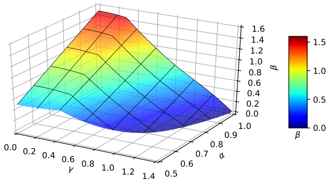
Refer to caption

Refer to caption Refer to caption

Figure 1. Top left: Above the red line, 𝔸s,t\mathbb{A}_{s,t} is well-defined for given ss and tt, and satisfies the Chen relation (up to modification). Above the black curve, it admits a continuous modification. On the left of the red point, 𝔸s,t\mathbb{A}_{s,t} is well-defined for a Brownian motion, and satisfies the Chen relation. On the left of the black point, it admits a continuous modification. Remark the black dot is below the black curve. Top right, bottom left, bottom right: Lower bound on the exponent β=β⁡(α,γ)\beta=\beta(\alpha,\gamma) of regularity. The black curves on the bottom figures correspond to the values α=γ−2\alpha=\gamma^{-2} for which the expression of our lower bounds changes. The green curve in the bottom right figure corresponds to the values α=3−2​22​γ2\alpha=\frac{3-2\sqrt{2}}{2\gamma^{2}}, for which the expression of our lower bounds changes a second time. The red line on the bottom left figure is the correct value of β\beta in the classical case 𝖬=λ\mathsf{M}=\lambda (‘γ=0\gamma=0’)

During the proof, we will also show that 𝔸s,tY\mathbb{A}^{Y}_{s,t} is ‘stochastically 2​α2\alpha-regular’, in the following sense.

Theorem 5.

Assume that either γ∈[0,2)\gamma\in[0,2), α>12\alpha>\frac{1}{2} and ρ=1\rho=1, or that γ<2\gamma<\sqrt{2}, α>1ν\alpha>\frac{1}{\nu} and ρ∈[1,α​ν)\rho\in[1,\alpha\nu). Then, for all (s,t)∈Δ(s,t)\in\Delta, 𝔸s,tY\mathbb{A}^{Y}_{s,t} lies in Lρ​(Ω𝖬)L^{\rho}(\Omega^{\mathsf{M}}), and there exists a constant CC which does not depend on (s,t)(s,t) and such that ‖𝔸s,tY‖Lρ​(Ω𝖬)≤C​|t−s|2​α\|\mathbb{A}^{Y}_{s,t}\|_{L^{\rho}(\Omega^{\mathsf{M}})}\leq C|t-s|^{2\alpha}.

The two parts of the paper (Sections 1 to 5, Sections 6 to 10) are mostly independent, but reading Proposition 1.1 and Lemmas 2.1 and 2.2 is necessary to understand the second part.

1. Strategy of the proof of Theorem 1

Let us recall that X:[0,1]→ℝ2X:[0,1]\to\mathbb{R}^{2} is a planar Brownian motion defined on (ΩX,ℱX,ℙX)(\Omega^{X},\mathcal{F}^{X},\mathbb{P}^{X}), and θX\theta_{X} is the winding function associated with XX. The random measure 𝖬\mathsf{M} is defined on (Ω𝖬,ℱ𝖬,ℙ𝖬)(\Omega^{\mathsf{M}},\mathcal{F}^{\mathsf{M}},\mathbb{P}^{\mathsf{M}}), and is formally given by 𝖬=eγ​ϕ−γ22​𝔼​[ϕ2]​λ\mathsf{M}=e^{\gamma\phi-\frac{\gamma^{2}}{2}\mathbb{E}[\phi^{2}]}\lambda, where λ\lambda is the Lebesgue measure and ϕ\phi is a centered Gaussian field on ℝ2\mathbb{R}^{2} with covariance kernel K:(z,w)↦log+⁡(|z−w|)+g⁡(z,w)K:(z,w)\mapsto\log_{+}(|z-w|)+g(z,w), for a bounded 𝒞2\mathcal{C}^{2} function gg with bounded derivatives up to order 22. From now on and until Section 5 included, we will assume that γ<4/3\gamma<\sqrt{4/3}. We are looking at the existence of a limit, as K→+∞K\to+\infty, of the integral with ‘cut-off’

∫ℝ2max⁡(−K,min⁡(θX​(z),K))​𝑑z.\int_{\mathbb{R}^{2}}\max(-K,\min(\theta_{X}(z),K))\;{\rm d}z.

Since θX\theta_{X} takes its values in ℤ\mathbb{Z}, we can rewrite this integral as

∑n=−∞+∞max⁡(−K,min⁡(n,K))​𝖬​({z∈ℝ2:θX​(z)=n}),\sum_{n=-\infty}^{+\infty}\max(-K,\min(n,K))\mathsf{M}(\{z\in\mathbb{R}^{2}:\theta_{X}(z)=n\}),

which is more conveniently written

∑n=1+∞min⁡(n,K)​(𝖬⁡({z∈ℝ2:θX​(z)=n})−𝖬⁡({z∈ℝ2:θX​(z)=−n})).\sum_{n=1}^{+\infty}\min(n,K)\big(\mathsf{M}(\{z\in\mathbb{R}^{2}:\theta_{X}(z)=n\})-\mathsf{M}(\{z\in\mathbb{R}^{2}:\theta_{X}(z)=-n\})\big).

Performing a summation by parts, this is finally equal to

∑N=1K(𝖬⁡({z∈ℝ2:θX​(z)≥N})−𝖬⁡({z∈ℝ2:θX​(z)≤−N})).\sum_{N=1}^{K}\big(\mathsf{M}(\{z\in\mathbb{R}^{2}:\theta_{X}(z)\geq N\})-\mathsf{M}(\{z\in\mathbb{R}^{2}:\theta_{X}(z)\leq-N\})\big).

This is the expression we will study. We will show that the general term goes to zero sufficiently fast for the sum to be convergent. Consequently, for N≥1N\geq 1, we define the following sets:

(7) 𝒟N={z∈ℝ2∖Range⁡(X¯):θX​(z)≥N},𝒟−N={z∈ℝ2∖Range⁡(X¯):θX​(z)≤−N}.\mathcal{D}_{N}=\{z\in\mathbb{R}^{2}\setminus{\rm Range}(\bar{X}):\theta_{X}(z)\geq N\},\ \ \mathcal{D}_{-N}=\{z\in\mathbb{R}^{2}\setminus{\rm Range}(\bar{X}):\theta_{X}(z)\leq-N\}.

For a random variable ZZ on Ω\Omega, we set

‖Z‖p,q=‖Z‖Lp​(ΩX,Lq​(Ω𝖬))=𝔼X​[𝔼𝖬​[Zq]pq]1p.\|Z\|_{p,q}=\|Z\|_{L^{p}(\Omega^{X},L^{q}(\Omega^{\mathsf{M}}))}=\mathbb{E}^{X}[\mathbb{E}^{\mathsf{M}}[Z^{q}]^{\frac{p}{q}}]^{\frac{1}{p}}.

Theorem 1 is then a direct consequence of the following estimation.

Proposition 1.1.

For all p∈[2,4γ2)p\in[2,\frac{4}{\gamma^{2}}), there exists ε>0\varepsilon>0 and CC such that for all NN,

‖𝖬⁡(𝒟N)−𝖬⁡(𝒟−N)‖p,2≤C​N−1−ε.\|\mathsf{M}(\mathcal{D}_{N})-\mathsf{M}(\mathcal{D}_{-N})\|_{p,2}\leq CN^{-1-\varepsilon}.

Let us remark that this is only possible thanks to the compensation between 𝖬⁡(𝒟N)\mathsf{M}(\mathcal{D}_{N}) and 𝖬⁡(𝒟−N)\mathsf{M}(\mathcal{D}_{-N}). Indeed, each of these sets has a Lebesgue measure which is equivalent as NN tends ton infinity (in LqL^{q} for all qq, and in the almost sure sense) to 12​π​N\frac{1}{2\pi N}, so that even ‖𝖬⁡(𝒟N)‖p,1\|\mathsf{M}(\mathcal{D}_{N})\|_{p,1} is two large for the sum to be convergent. The fact that a compensation occurs can be informally understood as a consequence of the fact that the sets 𝒟N\mathcal{D}_{N} and 𝒟−N\mathcal{D}_{-N} are extremely similar when NN is large. For a better understanding of the asymptotic behaviour of 𝒟N\mathcal{D}_{N}, we refer to our article [14].

The strategy for the proof of Proposition 1.1 is similar to the one we used in [13] (Sections 3.2 and 3.3), and then in [14]. In short, we will decompose the quantity 𝖬⁡(𝒟N)\mathsf{M}(\mathcal{D}_{N}) into a sum of smaller quantities, corresponding to contributions of pieces of the Brownian trajectory.

To this end, we fix some t>0t>0, which should think of as being very small. For a positive integer NN, we set T=⌊Nt⌋T=\lfloor N^{t}\rfloor. For i∈{1,…,T}i\in\{1,\dots,T\}, we define XiX^{i} to be the restriction of XX to [(i−1)​T−1,i​T−1][(i-1)T^{-1},iT^{-1}], X¯i\bar{X}^{i} the concatenation of XiX^{i} with the segment between its endpoints, and θi​(z)\theta^{i}(z) the number of times X¯i\bar{X}^{i} winds around zz. We set

(8) 𝒟Ni={z∈ℝ2∖Range⁡(X¯i):θi​(z)≥N},𝒟−Ni={z∈ℝ2∖Range⁡(X¯i):θi​(z)≤−N}.\mathcal{D}^{i}_{N}=\{z\in\mathbb{R}^{2}\setminus\Range(\bar{X}^{i}):\theta^{i}(z)\geq N\},\ \ \mathcal{D}^{i}_{-N}=\{z\in\mathbb{R}^{2}\setminus\Range(\bar{X}^{i}):\theta^{i}(z)\leq-N\}.

Finally, we define

(9) 𝖬N=∑i=1T𝖬⁡(𝒟Ni).\mathsf{M}_{N}=\sum_{i=1}^{T}\mathsf{M}(\mathcal{D}^{i}_{N}).

This random variable should be thought of as a proxy for 𝖬⁡(𝒟N)\mathsf{M}(\mathcal{D}_{N}), when NN is large. To control the difference between 𝖬⁡(𝒟N)\mathsf{M}(\mathcal{D}_{N}) and 𝖬N\mathsf{M}_{N} will be the subject of Section 3, in which we will prove the following bound.

Proposition (3.7).

Let p∈(1,+∞)p\in(1,+\infty) and ε>0\varepsilon>0. Then, for tt small enough, there exists CC such that for all N≥1N\geq 1,

‖𝖬⁡(𝒟N)−𝖬N‖p,2≤C​N−3​ν4+2​t+ε.\|\mathsf{M}(\mathcal{D}_{N})-\mathsf{M}_{N}\|_{p,2}\leq CN^{-\frac{3\nu}{4}+2t+\varepsilon}.

In the case where the random measure 𝖬\mathsf{M} has a law invariant by translation, the variables 𝖬⁡(𝒟Ni)\mathsf{M}(\mathcal{D}^{i}_{N}) are identically distributed. If 𝖬\mathsf{M} also has a nice behaviour under scaling, then these variables are distributed as a scaled version of 𝖬⁡(𝒟N)\mathsf{M}(\mathcal{D}_{N}), and we end up with the informal relation

𝖬⁡(𝒟N)−𝖬⁡(𝒟−N)≃∑i=1T(𝖬⁡(𝒟Ni)−𝖬⁡(𝒟−Ni))=∑i=1Tf⁡(T)​Zi,\mathsf{M}(\mathcal{D}_{N})-\mathsf{M}(\mathcal{D}_{-N})\simeq\sum_{i=1}^{T}(\mathsf{M}(\mathcal{D}^{i}_{N})-\mathsf{M}(\mathcal{D}^{i}_{-N}))=\sum_{i=1}^{T}f(T)Z_{i},

where the ZiZ_{i} are random variables distributed as 𝖬⁡(𝒟N)−𝖬⁡(𝒟−N)\mathsf{M}(\mathcal{D}_{N})-\mathsf{M}(\mathcal{D}_{-N}). Let us assume that we can bound nicely the scaling function f⁡(T)f(T), and show that the variables ZiZ_{i} are not too strongly correlated. Then, inserting a bound on 𝖬⁡(𝒟N)−𝖬⁡(𝒟−N)\mathsf{M}(\mathcal{D}_{N})-\mathsf{M}(\mathcal{D}_{-N}) on the right-hand side might lead to a better bound on 𝖬⁡(𝒟N)−𝖬⁡(𝒟−N)\mathsf{M}(\mathcal{D}_{N})-\mathsf{M}(\mathcal{D}_{-N}). We refer to this as the bootstrap. The control on the correlation takes the following form.

Notation. The notation f⁡(N)≤Na+o⁡(1)f(N)\leq N^{a+o(1)} means that for all h>0h>0, there exists CC such that for all N≥1N\geq 1, f⁡(N)≤C​Na+hf(N)\leq CN^{a+h}.

Lemma (4.2).

For t,ε>0t,\varepsilon>0, and i,j∈{1,…,T}i,j\in\{1,\dots,T\}, let Fi,j={|X(i+1)​T−1−Xj​T−1|≥T−12+ε}F_{i,j}=\{|X_{(i+1)T^{-1}}-X_{jT^{-1}}|\geq T^{-\frac{1}{2}+\varepsilon}\}. For all p∈[2,4γ2)p\in\big[2,\frac{4}{\gamma^{2}}), there exists a constant CC such that for all N≥1N\geq 1,

(10) 𝔼X[|𝔼𝖬[∑i,j=1T𝟙Fi,j(𝖬(𝒟iN)−𝖬(𝒟i−N)(𝖬(𝒟jN)−𝖬(𝒟j−N))]|p2]1p≤C​log⁡(N+1)1p​Tε2​N−1​(N−14+o⁡(1)+Tγ24−1p).\mathbb{E}^{X}\big[\big|\mathbb{E}^{\mathsf{M}}\big[\sum_{i,j=1}^{T}\mathbbm{1}_{F_{i,j}}(\mathsf{M}(\mathcal{D}^{i}_{N})-\mathsf{M}(\mathcal{D}^{i}_{-N})(\mathsf{M}(\mathcal{D}^{j}_{N})-\mathsf{M}(\mathcal{D}^{j}_{-N}))\big]\big|^{\frac{p}{2}}\big]^{\frac{1}{p}}\\ \leq C\log(N+1)^{\frac{1}{p}}T^{\frac{\varepsilon}{2}}N^{-1}\big(N^{-\frac{1}{4}+o(1)}+T^{\frac{\gamma^{2}}{4}-\frac{1}{p}}\big).

The bootstrap then takes the following form. In the statement, there appears a set 𝒯⁡(𝖬)\mathcal{T}(\mathsf{M}) of random measures that will be defined precisely in Section 2. For the moment, suffice it to say that all the elements of 𝒯⁡(𝖬)\mathcal{T}(\mathsf{M}) look like 𝖬\mathsf{M}, in the sense that they are deduced from 𝖬\mathsf{M} by (possibly random) translations and symmetries. In many cases of interest, namely when gg is invariant by translation, 𝒪⁡(𝖬)={𝖬}\mathcal{O}(\mathsf{M})=\{\mathsf{M}\}.

Lemma (5.1).

Consider t>0,p∈[2,4ν]t>0,p\in[2,\frac{4}{\nu}] and ζ∈ℝ\zeta\in\mathbb{R}. Assume that there exists a constant CC such that for all 𝖬′∈𝒯⁡(𝖬)\mathsf{M}^{\prime}\in\mathcal{T}(\mathsf{M}) and all N≥1N\geq 1,

‖𝖬′​(𝒟N)−𝖬′​(𝒟−N)‖p,2≤C​Nζ.\|\mathsf{M}^{\prime}(\mathcal{D}_{N})-\mathsf{M}^{\prime}(\mathcal{D}_{-N})\|_{p,2}\leq CN^{\zeta}.

Then, for all ε>0\varepsilon>0, there exists a constant C′C^{\prime} such that for all N≥1N\geq 1,

𝔼X​[𝔼𝖬​[∑1≤i≤j≤T𝟙Fi,jc​|(𝖬⁡(𝒟Ni)−𝖬⁡(𝒟−Ni))​(𝖬⁡(𝒟Nj)−𝖬⁡(𝒟−Nj))|]p2]1p≤C′​log​(T+1)1p​Tγ24−1p+ε​Nζ.\mathbb{E}^{X}\big[\mathbb{E}^{\mathsf{M}}\big[\hskip-5.69046pt\sum_{1\leq i\leq j\leq T}\hskip-5.69046pt\mathbbm{1}_{F_{i,j}^{c}}|(\mathsf{M}(\mathcal{D}^{i}_{N})-\mathsf{M}(\mathcal{D}^{i}_{-N}))(\mathsf{M}(\mathcal{D}^{j}_{N})-\mathsf{M}(\mathcal{D}^{j}_{-N}))|\big]^{\frac{p}{2}}\big]^{\frac{1}{p}}\leq C^{\prime}\log(T+1)^{\frac{1}{p}}T^{\frac{\gamma^{2}}{4}-\frac{1}{p}+\varepsilon}N^{\zeta}.

These propositions, properly combined, will allow us to prove the theorem. During the proof, we will use the following estimation that we proved in [13, Theorem 1.5]. For a measurable set AA, the notation |A||A| always denotes the Lebesgue measure of AA.

Lemma 1.2.

For all p∈[2,+∞)p\in[2,+\infty) and all δ<12\delta<\frac{1}{2}, there exists a constant CC such that for all N∈ℕN\in\mathbb{N},

𝔼​[|N|​𝒟N​|−12​π|p]1p≤C​N−δ.\mathbb{E}\Big[\big|N|\mathcal{D}_{N}|-\frac{1}{2\pi}\big|^{p}\Big]^{\frac{1}{p}}\leq CN^{-\delta}.

The next section contains the material that will allow us to estimate the ℙ𝖬\mathbb{P}^{\mathsf{M}}-expectation of some functionals of 𝖬\mathsf{M}.

2. Three estimates about the Liouville measures

In this section, we assume that γ<2\gamma<\sqrt{2}. Recall that ν\nu is the positive real number

ν=2−γ22.\nu=2-\frac{\gamma^{2}}{2}.

One of the advantages of working in the L2L^{2}-phase (that is, under the assumption γ<2\gamma<\sqrt{2}) is that one has the following explicit formula.

Lemma 2.1.

Let A,BA,B be two Borel subsets of ℝ2\mathbb{R}^{2} with finite Lebesgue measure. Then,

𝔼𝖬​[𝖬⁡(A)​𝖬​(B)]=∫A×Bexp⁡(γ2​K​(z,w))​𝑑z​𝑑w.\mathbb{E}^{\mathsf{M}}[\mathsf{M}(A)\mathsf{M}(B)]=\int_{A\times B}\exp(\gamma^{2}K(z,w))\;{\rm d}z\;{\rm d}w.
Proof.

We first do an informal computation, which is entirely valid when the kernel KK is replaced with a continuous kernel K~\tilde{K} (in which case the centered Gaussian field ϕ\phi with kernel K~\tilde{K} is defined pointwise):

𝔼𝖬​[𝖬​(A)​𝖬​(B)]\displaystyle\mathbb{E}^{\mathsf{M}}[\mathsf{M}(A)\mathsf{M}(B)] =𝔼𝖬​[∫A×Beγ​ϕz−γ22​𝔼𝖬​[ϕz2]​eγ​ϕw−γ22​𝔼𝖬​[ϕw2]​𝑑z​𝑑w]\displaystyle=\mathbb{E}^{\mathsf{M}}\Big[\int_{A\times B}e^{\gamma\phi_{z}-\frac{\gamma^{2}}{2}\mathbb{E}^{\mathsf{M}}[\phi_{z}^{2}]}e^{\gamma\phi_{w}-\frac{\gamma^{2}}{2}\mathbb{E}^{\mathsf{M}}[\phi_{w}^{2}]}\;{\rm d}z\;{\rm d}w\Big]
=∫A×B𝔼𝖬​[eγ⁡(ϕz+ϕw)−γ22​𝔼𝖬​[(ϕz+ϕw)2]]​eγ2​K~​(z,w)​𝑑z​𝑑w\displaystyle=\int_{A\times B}\mathbb{E}^{\mathsf{M}}\big[e^{\gamma(\phi_{z}+\phi_{w})-\frac{\gamma^{2}}{2}\mathbb{E}^{\mathsf{M}}[(\phi_{z}+\phi_{w})^{2}]}\big]e^{\gamma^{2}\tilde{K}(z,w)}\;{\rm d}z\;{\rm d}w
=∫A×Beγ2​K~​(z,w)​𝑑z​𝑑w.\displaystyle=\int_{A\times B}e^{\gamma^{2}\tilde{K}(z,w)}\;{\rm d}z\;{\rm d}w.

For a smooth mollifier θ\theta and a centered Gaussian field Φ\Phi with kernel KK, we define θε\theta_{\varepsilon} as the function ε−2​θ​(⋅ε)\varepsilon^{-2}\theta(\tfrac{\cdot}{\varepsilon}), and Φε\Phi_{\varepsilon} as the convolution of Φ\Phi with θε\theta_{\varepsilon}. For a Borel measurable set AA with finite Lebesgue measure, set also

𝖬ε​(A)=∫Aeγ​Φε​(z)−γ22​𝔼​[(Φε​(z))2]​𝑑λ​(z).\mathsf{M}_{\varepsilon}(A)=\int_{A}e^{\gamma\Phi_{\varepsilon}(z)-\frac{\gamma^{2}}{2}\mathbb{E}[(\Phi_{\varepsilon}(z))^{2}]}\;{\rm d}\lambda(z).

Then, when ε→0\varepsilon\to 0, 𝖬ε​(A)\mathsf{M}_{\varepsilon}(A) converges in L2L^{2} toward 𝖬⁡(A)\mathsf{M}(A) (see for example [12, Theorem 2.3]44 4 The cited theorem states convergence in probability, without assuming γ<2\gamma<\sqrt{2}, but the proof is about the L2L^{2} convergence provided γ<2\gamma<\sqrt{2}. Remark that it is taken as a definition for the measure 𝖬\mathsf{M} (up to some argument to make it not only a collection of random variables, but a measure). The original construction of Kahane is rather different.).

It follows that for any two Lebesgue measurable sets AA and BB with finite Lebesgue measures,

𝔼𝖬​[𝖬⁡(A)​𝖬​(B)]=limε→0𝔼𝖬​[𝖬ε​(A)​𝖬ε​(B)].\mathbb{E}^{\mathsf{M}}[\mathsf{M}(A)\mathsf{M}(B)]=\lim_{\varepsilon\to 0}\mathbb{E}^{\mathsf{M}}[\mathsf{M}_{\varepsilon}(A)\mathsf{M}_{\varepsilon}(B)].

On the other hand, the previous computation shows that

𝔼𝖬​[𝖬ε​(A)​𝖬ε​(B)]\displaystyle\mathbb{E}^{\mathsf{M}}[\mathsf{M}_{\varepsilon}(A)\mathsf{M}_{\varepsilon}(B)] =∫A×Beγ2​𝔼𝖬​[Xε​(z)​Xε​(w)]​𝑑z​𝑑w\displaystyle=\int_{A\times B}e^{\gamma^{2}\mathbb{E}^{\mathsf{M}}[X_{\varepsilon}(z)X_{\varepsilon}(w)]}\;{\rm d}z\;{\rm d}w
⟶ε→0​∫A×Beγ2​K​(z,w)​𝑑z​𝑑w.\displaystyle\underset{\varepsilon\to 0}{\longrightarrow}\int_{A\times B}e^{\gamma^{2}K(z,w)}\;{\rm d}z\;{\rm d}w.

The last convergence follows from pointwise convergence of 𝔼⁡[Xε​(z)​Xε​(w)]\mathbb{E}[X_{\varepsilon}(z)X_{\varepsilon}(w)] toward K⁡(z,w)K(z,w), and dominated convergence theorem (see [12, Theorem 2.3] again). ∎

According to , the scaling properties of the measure 𝖬\mathsf{M} are such that, in the case where K⁡(z,w)=log+⁡(|z+w|−1)K(z,w)=\log_{+}(\ |z+w|^{-1}), for a set A⊂B⁡(0,12)A\subset B(0,\frac{1}{2}) and r<1r<1, we have

𝔼𝖬​[𝖬​(r​A)2]=r2​ν​𝔼𝖬​[𝖬​(A)2],\mathbb{E}^{\mathsf{M}}[\mathsf{M}(rA)^{2}]=r^{2\nu}\mathbb{E}^{\mathsf{M}}[\mathsf{M}(A)^{2}],

where ν\nu is the constant defined at the beginning of this section. We deduce that for each such set AA, there exists a constant CC such that for all r≤1r\leq 1,

𝔼𝖬​[𝖬​(r​A)2]≤C​|r​A|ν.\mathbb{E}^{\mathsf{M}}[\mathsf{M}(rA)^{2}]\leq C|rA|^{\nu}.

We can actually choose CC such that the two terms are equal. The following lemma states that the constant CC can be chosen to be uniform over all measurable sets AA.

Lemma 2.2.

There exists CC such that for all measurable set A⊂ℝ2A\subset\mathbb{R}^{2},

𝔼𝖬​[𝖬​(A)2]≤C⁡(|A|ν+|A|2).\mathbb{E}^{\mathsf{M}}[\mathsf{M}(A)^{2}]\leq C(|A|^{\nu}+|A|^{2}).
Proof.

From the previous lemma, we know that

𝔼𝖬​[𝖬​(A)2]=∫A2exp⁡(γ2​K​(z,w))​𝑑z​𝑑w.\mathbb{E}^{\mathsf{M}}[\mathsf{M}(A)^{2}]=\int_{A^{2}}\exp(\gamma^{2}K(z,w))\;{\rm d}z\;{\rm d}w.

Since K⁡(z,w)≤log+⁡(|z−w|−1)+cK(z,w)\leq\log_{+}(|z-w|^{-1})+c for some constant cc,

𝔼𝖬​[𝖬​(A)2]≤eγ2​c​∫A2exp⁡(γ2​log+⁡(|z−w|−1))​𝑑z​𝑑w=eγ2​c​∫A2max⁡(|z−w|−γ2,1)​𝑑z​𝑑w.\mathbb{E}^{\mathsf{M}}[\mathsf{M}(A)^{2}]\leq e^{\gamma^{2}c}\int_{A^{2}}\exp(\gamma^{2}\log_{+}(|z-w|^{-1}))\;{\rm d}z\;{\rm d}w=e^{\gamma^{2}c}\int_{A^{2}}\max(|z-w|^{-\gamma^{2}},1)\;{\rm d}z\;{\rm d}w.

Let r=|A|12​π−12r=|A|^{\frac{1}{2}}\pi^{-\frac{1}{2}} be the radius of a disk of the same area as AA, and

Sr=supA′:|A′|=π​r2∫A′max(|z|−γ2,1)dz.S_{r}=\sup_{A^{\prime}:|A^{\prime}|=\pi r^{2}}\int_{A^{\prime}}\max(|z|^{-\gamma^{2}},1)\;{\rm d}z.

The supremum is achieved by the ball B⁡(0,r)B(0,r). By considering separately the cases r≤1r\leq 1 and r≥1r\geq 1, we find that Sr≤2​π2−γ2​r2−γ2+π​r2S_{r}\leq\frac{2\pi}{2-\gamma^{2}}r^{2-\gamma^{2}}+\pi r^{2}.

By invariance under translations, SrS_{r} is also equal to

supw∈ℝ2supA′:|A′|=π​r2∫A′max(|z−w|−γ2,1)dz.\sup_{w\in\mathbb{R}^{2}}\sup_{A^{\prime}:|A^{\prime}|=\pi r^{2}}\int_{A^{\prime}}\max(|z-w|^{-\gamma^{2}},1)\;{\rm d}z.

Thus,

𝔼𝖬​[𝖬​(A)2]\displaystyle\mathbb{E}^{\mathsf{M}}[\mathsf{M}(A)^{2}] ≤eγ2​c​∫A2max⁡(|z−w|−γ2,1)​𝑑z​𝑑w\displaystyle\leq e^{\gamma^{2}c}\int_{A^{2}}\max(|z-w|^{-\gamma^{2}},1)\;{\rm d}z\;{\rm d}w
≤eγ2​c​|A|​Sr≤eγ2​c​(2​πγ222−γ2​|A|2−γ22+|A|2).\displaystyle\leq e^{\gamma^{2}c}|A|S_{r}\leq e^{\gamma^{2}c}\Big(\frac{2\pi^{\frac{\gamma^{2}}{2}}}{2-\gamma^{2}}|A|^{2-\frac{\gamma^{2}}{2}}+|A|^{2}\Big).

This concludes the proof. ∎

The next estimate, should be understood as a quantitative version of the following idea. Let first A1A_{1}, A2A_{2} and BB be three sets such that A1A_{1} and A2A_{2} are very close from each other, have comparable Lebesgue measures, and are far from BB; then, 𝔼𝖬​[𝖬⁡(A1)​𝖬​(B)]\mathbb{E}^{\mathsf{M}}[\mathsf{M}(A_{1})\mathsf{M}(B)] should be very close to 𝔼𝖬​[𝖬⁡(A2)​𝖬​(B)]\mathbb{E}^{\mathsf{M}}[\mathsf{M}(A_{2})\mathsf{M}(B)]. Let now A1A_{1}, A2A_{2}, B1B_{1}, and B2B_{2} be four sets such that

  • ⋄\scriptstyle\diamond

    A1A_{1} and A2A_{2} are very close from each other, and have comparable Lebesgue measures,

  • ⋄\scriptstyle\diamond

    B1B_{1} and B2B_{2} are very close from each other, and have comparable Lebesgue measures,

  • ⋄\scriptstyle\diamond

    The AiA_{i} are far from the BiB_{i}.

Then, the expectation 𝔼𝖬​[(𝖬⁡(A2)−𝖬⁡(A1))​(𝖬⁡(B2)−𝖬⁡(B1))]\mathbb{E}^{\mathsf{M}}[(\mathsf{M}(A_{2})-\mathsf{M}(A_{1}))(\mathsf{M}(B_{2})-\mathsf{M}(B_{1}))] should be even smaller than 𝔼𝖬​[(𝖬⁡(A2)−𝖬⁡(A1))​𝖬​(Bi)]\mathbb{E}^{\mathsf{M}}[(\mathsf{M}(A_{2})-\mathsf{M}(A_{1}))\mathsf{M}(B_{i})]. Remark that the control on the ‘four terms’ expectation should depend on the distance between the AiA_{i}, the distance between the BiB_{i}, the distance between AiA_{i} and BiB_{i}, the Lebesgue measure of these four sets, and finally the difference between their Lebesgue measure. Hence, we do not expect a very short bound to appear.

For two disjoint sets AA and BB, let us define

dsup​(A,B)\displaystyle d_{\sup}(A,B) =sup{d(z,z′):z∈A,z′∈B},\displaystyle=\sup\{d(z,z^{\prime}):z\in A,z^{\prime}\in B\},
dinf​(A,B)\displaystyle d_{\inf}(A,B) =min(inf{d(z,z′):z∈A,z′∈B},1),\displaystyle=\min(\inf\{d(z,z^{\prime}):z\in A,z^{\prime}\in B\},1),

as illustrated by Figure 2 below.

Figure 2. A typical position for the sets in Lemma 2.3, and some of the ‘distances’ between them. A typical choice for these sets would be A1=𝒟NiA_{1}=\mathcal{D}^{i}_{N}, A2=𝒟−NiA_{2}=\mathcal{D}^{i}_{-N}, B1=𝒟NjB_{1}=\mathcal{D}^{j}_{N}, and B2=𝒟−NjB_{2}=\mathcal{D}^{j}_{-N}.
Lemma 2.3.

There exists CC such that for all bounded Borel measurable sets A1,A2,B1,B2A_{1},A_{2},B_{1},B_{2} with 4​max⁡(dsup​(A1,A2),dsup​(B1,B2))≤dinf​(A1,B1)4\max(d_{\sup}(A_{1},A_{2}),d_{\sup}(B_{1},B_{2}))\leq d_{\inf}(A_{1},B_{1}) and |A1|,|A2|,|B1|,|B2|≤1|A_{1}|,|A_{2}|,|B_{1}|,|B_{2}|\leq 1,

(11) |𝔼𝖬[(𝖬(A1)−𝖬(A2))(𝖬(B1)−𝖬(B2)]|≤C(dinf(A1,B1)−γ2||B1|−|B2||||A1|−|A2||+(dsup​(A1,A2)+dsup​(B1,B2))​dinf​(A1,B1)−1−γ2​(|A1​‖|B1|−|B2|​|+||A2|−|​A1|‖​B1|)OPEN+dinf​(A1,B1)−2−γ2​dsup​(A1,A2)​dsup​(B1,B2)​|A1|​|B1|).|\mathbb{E}^{\mathsf{M}}[(\mathsf{M}(A_{1})-\mathsf{M}(A_{2}))(\mathsf{M}(B_{1})-\mathsf{M}(B_{2})]|\leq C\Big(d_{\inf}(A_{1},B_{1})^{-\gamma^{2}}\big||B_{1}|-|B_{2}|\big|\big||A_{1}|-|A_{2}|\big|\\ +\big(d_{\sup}(A_{1},A_{2})+d_{\sup}(B_{1},B_{2})\big)d_{\inf}(A_{1},B_{1})^{-1-\gamma^{2}}\big(|A_{1}|\big||B_{1}|-|B_{2}|\big|+\big||A_{2}|-|A_{1}|\big||B_{1}|\big)\\ +d_{\inf}(A_{1},B_{1})^{-2-\gamma^{2}}d_{\sup}(A_{1},A_{2})d_{\sup}(B_{1},B_{2})|A_{1}||B_{1}|\Big).

Let us remark that the exponent γ\gamma, which is carried by |A||A| when looking at 𝔼𝖬​[𝖬​(A)2]\mathbb{E}^{\mathsf{M}}[\mathsf{M}(A)^{2}], is here carried instead by dinf​(A1,B1)d_{\inf}(A_{1},B_{1}). Remark also that all these terms but the last vanish if |A1|=|A2||A_{1}|=|A_{2}| and |B1|=|B2||B_{1}|=|B_{2}|.

Proof.

It is a simple computation. Using the explicit formula given by Lemma 2.1, we have

𝔼𝖬[(𝖬(A1)−𝖬(A2))(𝖬(B1)−𝖬(B2)]\displaystyle\mathbb{E}^{\mathsf{M}}[(\mathsf{M}(A_{1})-\mathsf{M}(A_{2}))(\mathsf{M}(B_{1})-\mathsf{M}(B_{2})] =∫A1×B1eγ​K​(z1,w1)​d​z1​d​w1−∫A1×B2eγ​K​(z1,w2)​d​z1​d​w2\displaystyle=\int_{A_{1}\times B_{1}}e^{\gamma K(z_{1},w_{1})}\;{\rm d}z_{1}\;{\rm d}w_{1}-\int_{A_{1}\times B_{2}}e^{\gamma K(z_{1},w_{2})}\;{\rm d}z_{1}\;{\rm d}w_{2}
−∫A2×B1eγ​K​(z2,w1)dz2dw1+∫A2×B2eγ​K​(z2,w2)dz2dw2\displaystyle\hskip 28.45274pt-\int_{A_{2}\times B_{1}}e^{\gamma K(z_{2},w_{1})}\;{\rm d}z_{2}\;{\rm d}w_{1}+\int_{A_{2}\times B_{2}}e^{\gamma K(z_{2},w_{2})}\;{\rm d}z_{2}\;{\rm d}w_{2}

Writing Q=A1×A2×B1×B2Q=A_{1}\times A_{2}\times B_{1}\times B_{2}, the right-hand side of this equation is equal to

1|Q|​∫Q(|A1|​|B1|​(eγ​K​(z1,w1)−eγ​K​(z1,w2)−eγ​K​(z2,w1)+eγ​K​(z2,w2))CLOSE+|A1|​(|B2|−|B1|)​(eγ​K​(z2,w2)−eγ​K​(z1,w2))+(|A2|−|A1|)​|B1|​(eγ​K​(z2,w2)−eγ​K​(z2,w1))OPEN+(|A2|−|A1|)​(|B2|−|B1|)​eγ​K​(z2,w2))​d​z1​d​z2​d​w1​d​w2.\frac{1}{|Q|}\int_{Q}\Big(|A_{1}||B_{1}|(e^{\gamma K(z_{1},w_{1})}-e^{\gamma K(z_{1},w_{2})}-e^{\gamma K(z_{2},w_{1})}+e^{\gamma K(z_{2},w_{2})})\\ +|A_{1}|(|B_{2}|-|B_{1}|)(e^{\gamma K(z_{2},w_{2})}-e^{\gamma K(z_{1},w_{2})})+(|A_{2}|-|A_{1}|)|B_{1}|(e^{\gamma K(z_{2},w_{2})}-e^{\gamma K(z_{2},w_{1})})\\ +(|A_{2}|-|A_{1}|)(|B_{2}|-|B_{1}|)e^{\gamma K(z_{2},w_{2})}\Big)\;{\rm d}z_{1}\;{\rm d}z_{2}\;{\rm d}w_{1}\;{\rm d}w_{2}.

This, in absolute value, is less than

sup(z1,z2,w1,w2)∈Q(CLOSE\displaystyle\sup_{(z_{1},z_{2},w_{1},w_{2})\in Q}\Big( |A1|​|B1|​|eγ​K​(z1,w1)−eγ​K​(z1,w2)−eγ​K​(z2,w1)+eγ​K​(z2,w2)|\displaystyle|A_{1}||B_{1}||e^{\gamma K(z_{1},w_{1})}-e^{\gamma K(z_{1},w_{2})}-e^{\gamma K(z_{2},w_{1})}+e^{\gamma K(z_{2},w_{2})}|
+|A1​‖|B2​|−|B1​‖|eγ​K​(z2,w2)−eγ​K​(z1,w2)|+‖​A2|−|​A1|‖​B1|​|eγ​K​(z2,w2)−eγ​K​(z2,w1)|\displaystyle+|A_{1}|\big||B_{2}|-|B_{1}|\big||e^{\gamma K(z_{2},w_{2})}-e^{\gamma K(z_{1},w_{2})}|+\big||A_{2}|-|A_{1}|\big||B_{1}||e^{\gamma K(z_{2},w_{2})}-e^{\gamma K(z_{2},w_{1})}|
OPEN+||A2|−|​A1​‖||B2|−|​B1‖​eγ​K​(z2,w2)).\displaystyle\hskip 170.71652pt+\big||A_{2}|-|A_{1}|\big|\big||B_{2}|-|B_{1}|\big|e^{\gamma K(z_{2},w_{2})}\Big).

We set DAD_{A} a ball of diameter dsup​(A1,A2)d_{\sup{}}(A_{1},A_{2}) containing A1A_{1} and A2A_{2}, and DBD_{B} a ball of diameter dsup​(B1,B2)d_{\sup{}}(B_{1},B_{2}) containing B1B_{1} and B2B_{2}, so tat the last expression is less than

|A1|​|B1|​dsup​(A1,A2)​dsup​(B1,B2)​supz∈DA,w∈DB‖∇2eγ​K​(z,w)‖+|A1|||B2|−|B1||​dsup​(A1,A2)​supz∈DA,w2∈B2‖∇eγ​K​(z,w2)‖+||A2|−|A1|||B1|​dsup​(B1,B2)​supz2∈A2,w∈DB‖∇eγ​K​(z2,w)‖+||A2|−|A1​‖||B2|−|​B1‖​supz2∈A2,w2∈B2eγ​K​(z2,w2).|A_{1}||B_{1}|d_{\sup{}}(A_{1},A_{2})d_{\sup{}}(B_{1},B_{2})\sup_{z\in D_{A},w\in D_{B}}\|\nabla^{2}e^{\gamma K(z,w)}\|\\ +|A_{1}|\big||B_{2}|-|B_{1}|\big|d_{\sup{}}(A_{1},A_{2})\sup_{z\in D_{A},w_{2}\in B_{2}}\|\nabla e^{\gamma K(z,w_{2})}\|\\ +\big||A_{2}|-|A_{1}|\big||B_{1}|d_{\sup{}}(B_{1},B_{2})\sup_{z_{2}\in A_{2},w\in D_{B}}\|\nabla e^{\gamma K(z_{2},w)}\|\\ +\big|\!|A_{2}|-|A_{1}|\!\big|\big|\!|B_{2}|-|B_{1}|\!\big|\sup_{z_{2}\in A_{2},w_{2}\in B_{2}}e^{\gamma K(z_{2},w_{2})}.

The three suprema appearing in this expression are respectively less than C​dinf​(DA,DB)−2−γ2Cd_{\inf{}}(D_{A},D_{B})^{-2-\gamma^{2}}, C​dinf​(DA,B2)−1−γ2Cd_{\inf{}}(D_{A},B_{2})^{-1-\gamma^{2}} and C​dinf​(A2,B2)−γ2Cd_{\inf{}}(A_{2},B_{2})^{-\gamma^{2}}, where the constant CC depends on the exact expression of the kernel KK but not on the four sets A1A_{1},A2A_{2},B1B_{1},B2B_{2}.

Since dinf​(DA,DB)≥dinf​(A1,B1)−dsup​(A1,A2)−dsup​(B1,B2)≥12​dinf​(A1,B1)d_{\inf{}}(D_{A},D_{B})\geq d_{\inf{}}(A_{1},B_{1})-d_{\sup{}}(A_{1},A_{2})-d_{\sup{}}(B_{1},B_{2})\geq\frac{1}{2}d_{\inf{}}(A_{1},B_{1}), we deduce the announced inequality.

∎

For reasons that will appear only at the end of the proof, we need to consider not only the random measure 𝖬\mathsf{M}, but also measures obtained by possibly random (but independent from 𝖬\mathsf{M}) translation of 𝖬\mathsf{M}.

For z∈ℝ2z\in\mathbb{R}^{2}, we define the random measure τz​(𝖬)\tau_{z}(\mathsf{M}) by setting, for all Borel measurable set AA,

τz​(𝖬)​(A)=𝖬⁡(A+z).\lx@nobreakspace\tau_{z}(\mathsf{M})(A)=\mathsf{M}(A+z).

For a probability law pp on ℝ2\mathbb{R}^{2}, we also set τp​(𝖬)=∫ℝ2τz​(𝖬)​𝑑p​(z)\tau_{p}(\mathsf{M})=\int_{\mathbb{R}^{2}}\tau_{z}(\mathsf{M})\;{\rm d}p(z). Finally, we define

𝒯⁡(𝖬)={τp​(𝖬):p​ is a probability law on ​ℝ2}.\mathcal{T}(\mathsf{M})=\{\tau_{p}(\mathsf{M}):p\mbox{ is a probability law on }\mathbb{R}^{2}\}.

For a random measure 𝖬~\tilde{\mathsf{M}}, let us define

‖|𝖬~|‖0\displaystyle|\!|\!|\tilde{\mathsf{M}}|\!|\!|_{0} =inf{C>0:∀A Borel set with |A|≤1,𝔼𝖬[𝖬~(A)2]≤C|A|ν}12\displaystyle=\inf\big\{C>0:\forall A\text{ Borel set with }|A|\leq 1,\ \mathbb{E}^{\mathsf{M}}[\tilde{\mathsf{M}}(A)^{2}]\leq C|A|^{\nu}\big\}^{\frac{1}{2}}
=inf{C>0: Lemma 2.2 holds}12\displaystyle=\inf\big\{C>0:\text{ Lemma \ref{le:firstBound} holds}\}^{\frac{1}{2}}

and, similarly55 5 We chose this notation because it is related to the second derivatives of the kernel KK.,

‖|𝖬~|‖2=inf{C>0: Lemma 2.3 holds}12.|\!|\!|\tilde{\mathsf{M}}|\!|\!|_{2}=\inf\big\{C>0:\text{ Lemma \ref{le:4points} holds}\}^{\frac{1}{2}}.

It is easily shown that, for all 𝖬~∈𝒯⁡(𝖬)\tilde{\mathsf{M}}\in\mathcal{T}(\mathsf{M}), ‖|𝖬~|‖0≤‖|𝖬|‖0|\!|\!|\tilde{\mathsf{M}}|\!|\!|_{0}\leq|\!|\!|\mathsf{M}|\!|\!|_{0} and ‖|𝖬~|‖2≤‖|𝖬|‖2|\!|\!|\tilde{\mathsf{M}}|\!|\!|_{2}\leq|\!|\!|\mathsf{M}|\!|\!|_{2}.

In the following two sections, all the results stated with 𝖬\mathsf{M} also hold for any measure 𝖬~∈𝒯⁡(𝖬)\tilde{\mathsf{M}}\in\mathcal{T}(\mathsf{M}), with the same constants. Actually, they hold for all random measure 𝖬~\tilde{\mathsf{M}} with ‖|𝖬~|‖0<+∞|\!|\!|\tilde{\mathsf{M}}|\!|\!|_{0}<+\infty and ‖|𝖬~|‖2<+∞|\!|\!|\tilde{\mathsf{M}}|\!|\!|_{2}<+\infty. Furthermore, they hold uniformly on 𝒯⁡(𝖬)\mathcal{T}(\mathsf{M}) provided the constants CC are replaced with C⁡(|‖𝖬~‖|0+|​‖𝖬~‖|2)C(|\!|\!|\tilde{\mathsf{M}}|\!|\!|_{0}+|\!|\!|\tilde{\mathsf{M}}|\!|\!|_{2}).

3. Comparing 𝖬⁡(𝒟N)\mathsf{M}(\mathcal{D}_{N}) and 𝖬N\mathsf{M}_{N}

Let us recall the notation that we introduced in Section 1. We fix t>0t>0, a small positive real. We also fix a (large) positive integer NN, and define T=⌊Nt⌋T=\lfloor N^{t}\rfloor. In the estimations that follow, tt is going to be fixed, and NN is going to tend to infinity.

For each i∈{1,…,T}i\in\{1,\dots,T\}, we define

  • ⋄\scriptstyle\diamond

    XiX^{i} to be the restriction of XX to [(i−1)​T−1,i​T−1][(i-1)T^{-1},iT^{-1}],

  • ⋄\scriptstyle\diamond

    X¯i\bar{X}^{i} the concatenation of XiX^{i} with the segment between its endpoints,

  • ⋄\scriptstyle\diamond

    θi​(z)\theta^{i}(z) the number of times X¯i\bar{X}^{i} winds around zz,

  • ⋄\scriptstyle\diamond

    𝒟Ni={z∈ℝ2∖Range⁡(X¯i):θi​(z)≥N}\mathcal{D}^{i}_{N}=\{z\in\mathbb{R}^{2}\setminus\Range(\bar{X}^{i}):\theta^{i}(z)\geq N\}.

We then define

𝖬N=∑i=1T𝖬⁡(𝒟Ni).\mathsf{M}_{N}=\sum_{i=1}^{T}\mathsf{M}(\mathcal{D}^{i}_{N}).

Let us stress the fact that the law of the random sets 𝒟Ni\mathcal{D}^{i}_{N} can be deduced from that of 𝒟N\mathcal{D}_{N} by a scaling and a random translation. This self-similar behaviour will come into play in a crucial way in Section 5.

As explained in Section 1, one of our main objects of interest is 𝖬⁡(𝒟N)\mathsf{M}(\mathcal{D}_{N}), the 𝖬\mathsf{M}-measure of the set of points around which the Brownian motion winds at least NN times (see (7)), and our strategy to study it is to compare it with 𝖬N\mathsf{M}_{N}.

The goal of this section is to prove that 𝖬⁡(𝒟N)\mathsf{M}(\mathcal{D}_{N}) and 𝖬N\mathsf{M}_{N} are close, in the sense of Proposition 3.7. This result will allow us, in Section 5, to transfer to 𝖬⁡(𝒟N)\mathsf{M}(\mathcal{D}_{N}) the information about 𝖬N\mathsf{M}_{N} that we will gather in Section 4.

To compare 𝖬⁡(𝒟N)\mathsf{M}(\mathcal{D}_{N}) and 𝖬N\mathsf{M}_{N}, we introduce several sets. To start with, let us denote by ℰ\mathcal{E} the union of the range of X¯\bar{X} and the TT segments joining the endpoints of XiX^{i} for i∈{1,…,T}i\in\{1,\ldots,T\}. It is an important fact for us that this set ℰ\mathcal{E} is Lebesgue-negligible, and this implies that it is ℙ𝖬\mathbb{P}^{\mathsf{M}}-almost surely 𝖬\mathsf{M}-negligible. Then, given integers N,M1,M2N,M_{1},M_{2}, indices i,j∈{1,…,T}i,j\in\{1,\dots,T\}, and a multi-index 𝐢∈𝐈k={(i1,…,ik)∈{1,…,T}k:i1<⋯<ik}\mathbf{i}\in\mathbf{I}_{k}=\{(i_{1},\dots,i_{k})\in\{1,\dots,T\}^{k}:i_{1}<\dots<i_{k}\}, we define

𝒟N,M1i,j\displaystyle\mathcal{D}^{i,j}_{N,M_{1}} ={z∈ℝ2∖ℰ:|θi(z)|≥N,|θj(z)|≥M1},\displaystyle=\{z\in\mathbb{R}^{2}\setminus\mathcal{E}:|\theta^{i}(z)|\geq N,|\theta^{j}(z)|\geq M_{1}\},
𝒟M2𝐢\displaystyle\mathcal{D}^{\mathbf{i}}_{M_{2}} ={z∈ℝ2∖ℰ:∀l∈{1,…,k},|θil(z)|≥M2}.\displaystyle=\{z\in\mathbb{R}^{2}\setminus\mathcal{E}:\forall l\in\{1,\dots,k\},|\theta^{i_{l}}(z)|\geq M_{2}\}.

The integer kk that we will use will only depend on γ\gamma, and can be though of as being fixed.

The following lemma gives us a relation between the set 𝒟N\mathcal{D}_{N} and the sets that we just defined.

Lemma 3.1.

Assume that T​M2≤Nk−TTM_{2}\leq\frac{N}{k}-T and k​M1+(M2+1)​T<NkM_{1}+(M_{2}+1)T<N. Then,

⋃i=1T𝒟N+T​M1i∖⋃i≠j𝒟Nk,M1i,j⊆𝒟N∖ℰ⊆⋃i=1T𝒟N−k​M1−(M2+1)​Ti∪⋃i≠j𝒟Nk,M1i,j∪⋃𝐢∈𝐈k𝒟M2𝐢.\bigcup_{i=1}^{T}\mathcal{D}^{i}_{N+TM_{1}}\setminus\bigcup_{i\neq j}\mathcal{D}^{i,j}_{\frac{N}{k},M_{1}}\ \subseteq\ \mathcal{D}_{N}\setminus\mathcal{E}\ \subseteq\ \bigcup_{i=1}^{T}\mathcal{D}^{i}_{N-kM_{1}-(M_{2}+1)T}\cup\bigcup_{i\neq j}\mathcal{D}^{i,j}_{\frac{N}{k},M_{1}}\cup\bigcup_{\mathbf{i}\in\mathbf{I}_{k}}\mathcal{D}^{\mathbf{i}}_{M_{2}}.

These inclusions are purely deterministic and the statement remains true if replace the Brownian curve with any other curve. The proof is based on a discussion of the highest values taken by the winding functions of the pieces of our curve. It would probably be best done by the reader for himself, but we offer a detailed argument for the second inclusion, which is the less simple one.

Proof.

For a given point z∈ℝ2∖ℰz\in\mathbb{R}^{2}\setminus\mathcal{E}, let us sort the values (|θi​(z)|)i∈{1,…,T}(|\theta^{i}(z)|)_{i\in\{1,\dots,T\}} in non-increasing order and denote them by η1≥⋯≥ηT\eta_{1}\geq\dots\geq\eta_{T}. Let us also denote η~1\tilde{\eta}_{1} one of the values (θi​(z))i∈{1,…,T}(\theta^{i}(z))_{i\in\{1,\dots,T\}} such that |η~1|=η1|\tilde{\eta}_{1}|=\eta_{1}. We have the following implications:

z∉⋃i=1T𝒟N−k​M1−(M2+1)​Ti\displaystyle\textstyle z\notin\bigcup_{i=1}^{T}\mathcal{D}^{i}_{N-kM_{1}-({M_{2}}+1)T} ⟹η~1<N−k​M1−(M2+1)​T,\displaystyle\ \Longrightarrow\ \tilde{\eta}_{1}<N-kM_{1}-({M_{2}}+1)T,
z∉⋃𝐢∈𝐈k𝒟M2𝐢\displaystyle\textstyle z\notin\bigcup_{\mathbf{i}\in\mathbf{I}_{k}}\mathcal{D}^{\mathbf{i}}_{M_{2}} ⟹ηk<M2,\displaystyle\ \Longrightarrow\ \eta_{k}<{M_{2}},
z∉⋃i≠j𝒟Nk,M1i,j\displaystyle\textstyle z\notin\bigcup_{i\neq j}\mathcal{D}^{i,j}_{\frac{N}{k},M_{1}} ⟹(η1<Nk​ or ​η2<M1).\displaystyle\ \Longrightarrow\ \big(\eta_{1}<\tfrac{N}{k}\mbox{ or }\eta_{2}<M_{1}\big).

If zz is in none of the sets appearing on the left of these implications, we are in one of two cases, depending on which of the two assertions on the right of the third implication holds.

If η1<Nk\eta_{1}<\frac{N}{k}, then η2,…,ηk−1<Nk\eta_{2},\ldots,\eta_{k-1}<\frac{N}{k} and

∑i=1Tθi​(z)≤∑i=1Tηi<(k−1)​Nk+(T−(k−1))​M2≤N−T.\sum_{i=1}^{T}\theta^{i}(z)\leq\sum_{i=1}^{T}\eta_{i}<(k-1)\frac{N}{k}+(T-(k-1)){M_{2}}\leq N-T.

If η2<M1\eta_{2}<M_{1}, then η3,…,ηk−1<M1\eta_{3},\dots,\eta_{k-1}<M_{1} and

∑i=1Tθi​(z)≤η~1+∑i=2Tηi<(N−k​M1−(M2+1)​T)+(k−2)​M1+(T−(k−1))​M2≤N−T.\sum_{i=1}^{T}\theta^{i}(z)\leq\tilde{\eta}_{1}+\sum_{i=2}^{T}\eta_{i}<(N-kM_{1}-({M_{2}}+1)T)+(k-2)M_{1}+(T-(k-1)){M_{2}}\leq N-T.

In both cases, we conclude that ∑i=1Tθi​(z)≤N−T\sum_{i=1}^{T}\theta^{i}(z)\leq N-T. The difference between this sum and θX​(z)\theta_{X}(z) is the winding at zz of a piecewise linear curve with T+1T+1 pieces, which cannot exceed T−1T-1. Thus θX​(z)<N\theta_{X}(z)<N, so that z∉𝒟Nz\notin\mathcal{D}_{N}. ∎

In order to compare 𝖬⁡(𝒟N)\mathsf{M}(\mathcal{D}_{N}) with 𝖬N\mathsf{M}_{N}, we are going to take the 𝖬\mathsf{M}-measures of the sets of which we just proved the inclusion. The 𝖬\mathsf{M}-measures of the first unions appearing in the leftmost and rightmost terms of Lemma 3.1 will be close, but not exactly equal, to 𝖬N\mathsf{M}_{N}.

A first difference is that we are taking the measure of a union instead of the sum of the measures. This problem turns out not to be a serious one, and will be treated in the proof of Proposition 3.7.

A second difference is that instead of 𝖬N\mathsf{M}_{N}, there seems to appear 𝖬N′\mathsf{M}_{N^{\prime}} for two integers N′N^{\prime} close to NN. To go around this difficulty, we will in fact apply Lemma 3.1 to several well-chosen values of NN, and use Lemma 3.4 to connect the various estimations that we obtain in this way.

A third difference is that there are correction terms appearing on both sides, and which we need to control: this will be done by the following Lemma 3.2 and Corollary 3.3.

The first estimation in the next statement is a mild reformulation of the Lemma 2.4 that we obtained in [13]. The second one is a slight improvement of the Lemma 2.5 in the same paper, which corresponds to the case k=3k=3. The extension from k=3k=3 to general kk is obtain by following the same proof. It is a long, but elementary, computation that involves a decomposition of (ℝ2)k−1(\mathbb{R}^{2})^{k-1} into a family of products of balls and complementary of balls in ℝ2\mathbb{R}^{2}.

Lemma 3.2.

For all positive integer kk and all r∈(0,+∞)r\in(0,+\infty), there exists CC such that for all positive integers N,M1,M2N,M_{1},M_{2} and TT, the following holds.

  • ⋄\scriptstyle\diamond

    For all i,j∈{1,…,T},i≠ji,j\in\{1,\dots,T\},i\neq j,

    𝔼X​[|𝒟N,M1i,j|r]≤C​log⁡(T​N​M1+1)3​r+1​(T​N​M1)−r|j−i|+1.\mathbb{E}^{X}[|\mathcal{D}^{i,j}_{N,M_{1}}|^{r}]\leq C\log(TNM_{1}+1)^{3r+1}\frac{(TNM_{1})^{-r}}{|j-i|+1}.\hskip 42.67912pt
  • ⋄\scriptstyle\diamond

    For all 𝐢∈𝐈k\mathbf{i}\in\mathbf{I}_{k},

    𝔼X​[|𝒟M2𝐢|r]≤C​log⁡(M2​T+1)(k+1)​(r+1)−2​T−r​M2−k​r∏j=1k−1(ij+1−ij+1).\mathbb{E}^{X}[|\mathcal{D}^{\mathbf{i}}_{M_{2}}|^{r}]\leq C\log(M_{2}T+1)^{(k+1)(r+1)-2}\frac{T^{-r}M_{2}^{-kr}}{\prod_{j=1}^{k-1}(i_{j+1}-i_{j}+1)}.

From these estimations, Lemma 2.2 allows us to deduce corresponding estimations in the Liouville case. We then sum over i≠ji\neq j or over 𝐢\mathbf{i}, and we obtain the following result.

Corollary 3.3.

For all positive integer kk, for all p∈[1,+∞)p\in[1,+\infty), there exists a constant CC such that for all positive integers N,M1,M2,TN,M_{1},M_{2},T,

∑i≠j‖𝖬⁡(𝒟N,M1i,j)‖p,2\displaystyle\sum_{i\neq j}\|\mathsf{M}(\mathcal{D}^{i,j}_{N,M_{1}})\|_{p,2} ≤C​log⁡(T​N​M1+1)3​ν2+1p​T2−1p−ν2​N−ν2​M1−ν2,\displaystyle\leq C\log(TNM_{1}+1)^{\frac{3\nu}{2}+\frac{1}{p}}T^{2-\frac{1}{p}-\frac{\nu}{2}}N^{-\frac{\nu}{2}}M_{1}^{-\frac{\nu}{2}},
∑𝐢∈𝐈k‖𝖬⁡(𝒟M2𝐢)‖p,2\displaystyle\sum_{\mathbf{i}\in\mathbf{I}_{k}}\|\mathsf{M}(\mathcal{D}^{\mathbf{i}}_{M_{2}})\|_{p,2} ≤C​log⁡(M2​T+1)(k+1)​(ν2+1p)−2​Tk−kp−ν2​M2−k​ν2.\displaystyle\leq C\log(M_{2}T+1)^{(k+1)(\frac{\nu}{2}+\frac{1}{p})-2}T^{k-\frac{k}{p}-\frac{\nu}{2}}M_{2}^{-k\frac{\nu}{2}}.
Proof.

We prove the first inequality, the second proof is identical. For i≠ji\neq j, by Lemma 2.2,

𝔼𝖬​[𝖬​(𝒟N,M1i,j)2]12≤C⁡(|𝒟N,M1i,j|ν2+|𝒟N,M1i,j|).\mathbb{E}^{\mathsf{M}}[\mathsf{M}(\mathcal{D}^{i,j}_{N,M_{1}})^{2}]^{\frac{1}{2}}\leq C(|\mathcal{D}^{i,j}_{N,M_{1}}|^{\frac{\nu}{2}}+|\mathcal{D}^{i,j}_{N,M_{1}}|).

Applying Lemma 3.2 with r=p​ν2r=\frac{p\nu}{2} and with r=pr=p, we obtain

𝔼X​[𝔼𝖬​[𝖬​(𝒟N,M1i,j)2]p2]1p\displaystyle\mathbb{E}^{X}[\mathbb{E}^{\mathsf{M}}[\mathsf{M}(\mathcal{D}^{i,j}_{N,M_{1}})^{2}]^{\frac{p}{2}}]^{\frac{1}{p}} ≤C′​𝔼X​[|𝒟N,M1i,j|p​ν2+|𝒟N,M1i,j|p]1p\displaystyle\leq C^{\prime}\mathbb{E}^{X}[|\mathcal{D}^{i,j}_{N,M_{1}}|^{\frac{p\nu}{2}}+|\mathcal{D}^{i,j}_{N,M_{1}}|^{p}]^{\frac{1}{p}}
≤C′′​log⁡(T​N​M1+1)3​ν2+1p​(T​N​M1)−ν2(|j−i|+1)1p.\displaystyle\leq C^{\prime\prime}\log(TNM_{1}+1)^{\frac{3\nu}{2}+\frac{1}{p}}\frac{(TNM_{1})^{-\frac{\nu}{2}}}{(|j-i|+1)^{\frac{1}{p}}}.

We then sum over i≠ji\neq j to get the announced bound. ∎

The next lemma compares the measures of 𝒟N\mathcal{D}_{N} and 𝒟N′\mathcal{D}_{N^{\prime}} when NN and N′N^{\prime} are close.

Lemma 3.4.

Let M=M⁡(N)M=M(N) be an integer-valued function of NN such that M→∞M\to\infty and MN→0\frac{M}{N}\to 0 as NN tends to infinity. Then, for all r∈(0,+∞)r\in(0,+\infty),

𝔼X​[||𝒟N|−|𝒟N+M||r]1r≤O⁡(M​N−2)+M2r​N−32−1r+o⁡(1).\mathbb{E}^{X}\big[\big||\mathcal{D}_{N}|-|\mathcal{D}_{N+M}|\big|^{r}\big]^{\frac{1}{r}}\leq O(MN^{-2})+M^{\frac{2}{r}}N^{-\frac{3}{2}-\frac{1}{r}+o(1)}.

If additionally lim infMqN>0\liminf\frac{M^{q}}{N}>0 for some q<2q<2, then for all r∈(0,+∞)r\in(0,+\infty), there exists CC such that for all N≥1N\geq 1,

𝔼X​[||𝒟N|−|𝒟N+M||r]1r≤C​M​N−2.\mathbb{E}^{X}\big[\big||\mathcal{D}_{N}|-|\mathcal{D}_{N+M}|\big|^{r}\big]^{\frac{1}{r}}\leq CMN^{-2}.
Proof.

We use the following convergence, which is the main result of [15].

(12) 𝔼X​[(n2​|{z∈ℝ2:θ⁡(z)=n}|−12​π)2]​⟶n→∞​0.\mathbb{E}^{X}\big[(n^{2}|\{z\in\mathbb{R}^{2}:\theta(z)=n\}|-\tfrac{1}{2\pi})^{2}\big]\underset{n\to\infty}{\longrightarrow}0.

In particular, there exists CC such that for all n≥1n\geq 1, 𝔼X​[|{z∈ℝ2:θ⁡(z)=n}|2]12≤C​n−2\mathbb{E}^{X}[|\{z\in\mathbb{R}^{2}:\theta(z)=n\}|^{2}]^{\frac{1}{2}}\leq Cn^{-2}. Summing from n=Nn=N to N+M−1N+M-1, we deduce that

(13) 𝔼X​[(|𝒟N|−|𝒟N+M|)2]12≤C​M​N−2.\mathbb{E}^{X}[(|\mathcal{D}_{N}|-|\mathcal{D}_{N+M}|)^{2}]^{\frac{1}{2}}\leq CMN^{-2}.

This is sufficient to conclude in the case r=2r=2. The case r<2r<2 follows from Hölder inequality. For r>2r>2, we fix some p>rp>r. From the triangle inequality,

𝔼X​[||𝒟N|−|𝒟N+M||p]1p≤𝔼X​[||𝒟N|−12​π​N|p]1p+𝔼X​[||𝒟N+M|−12​π​(N+M)|p]1p​M2​π​N​(N+M)\mathbb{E}^{X}\big[\big||\mathcal{D}_{N}|-|\mathcal{D}_{N+M}|\big|^{p}\big]^{\frac{1}{p}}\leq\mathbb{E}^{X}\big[\big||\mathcal{D}_{N}|-\tfrac{1}{2\pi N}\big|^{p}\big]^{\frac{1}{p}}+\mathbb{E}^{X}\big[\big||\mathcal{D}_{N+M}|-\tfrac{1}{2\pi(N+M)}\big|^{p}\big]^{\frac{1}{p}}\tfrac{M}{2\pi N(N+M)}

By Lemma 1.2, there is thus CC such that for all NN and MM,

(14) 𝔼X​[(|𝒟N|−|𝒟N+M|)p]1p≤C⁡(N−32+o⁡(1)+M​N−2).\mathbb{E}^{X}[(|\mathcal{D}_{N}|-|\mathcal{D}_{N+M}|)^{p}]^{\frac{1}{p}}\leq C(N^{-\frac{3}{2}+o(1)}+MN^{-2}).

We now interpolate between the inequalities (13) and (14). Setting θ=r−1−p−12−1−p−1\theta=\frac{r^{-1}-p^{-1}}{2^{-1}-p^{-1}}, the Hölder inequality is written

∥∙∥Lr≤∥∙∥L2θ∥∙∥Lp1−θ.\|\ {\raisebox{1.42271pt}{$\scriptscriptstyle\bullet$}}\ \|_{L^{r}}\leq\|\ {\raisebox{1.42271pt}{$\scriptscriptstyle\bullet$}}\ \|_{L^{2}}^{\theta}\|\ {\raisebox{1.42271pt}{$\scriptscriptstyle\bullet$}}\ \|_{L^{p}}^{1-\theta}.

Hence,

𝔼X​[(|𝒟N|−|𝒟N+M|)r]1r≤C⁡(M​N−2+(M​N−2)θ​(N−32−o⁡(1))1−θ).\mathbb{E}^{X}[(|\mathcal{D}_{N}|-|\mathcal{D}_{N+M}|)^{r}]^{\frac{1}{r}}\leq C\big(MN^{-2}+\big(MN^{-2}\big)^{\theta}(N^{-\frac{3}{2}-o(1)})^{1-\theta}\big).

As pp goes to infinity, θ\theta goes to 2r\frac{2}{r}, and we end up with

𝔼X​[(|𝒟N|−|𝒟N+M|)r]1r≤C⁡(M​N−2+M2r​N−32−1r+o⁡(1)).\mathbb{E}^{X}[(|\mathcal{D}_{N}|-|\mathcal{D}_{N+M}|)^{r}]^{\frac{1}{r}}\leq C\big(MN^{-2}+M^{\frac{2}{r}}N^{-\frac{3}{2}-\frac{1}{r}+o(1)}\big).

This is the first announced bound.

For the last bound, it suffices to remark that, for any r>2r>2, for ε\varepsilon small enough, M2r​N−32−1r+εM^{\frac{2}{r}}N^{-\frac{3}{2}-\frac{1}{r}+\varepsilon} is negligible compared to M​N−2MN^{-2}. ∎

Remark 3.5.

In [15], it is stated that the convergence (12) can be extended to higher moments, and the proof is sketched. We are convinced that this sketch can indeed, to the price of a lot of effort, be turned into a proof, but to the best of our knowledge, this has not been done. If this statement is true, as we think it is, the proof of Lemma 3.4 becomes almost trivial, and the additional assumption becomes superflous.

Corollary 3.6.

Let M=M⁡(N)M=M(N) be an integer-valued function of NN such that Mq​N−1→∞M^{q}N^{-1}\to\infty for some q<2q<2, and M​N−1→0MN^{-1}\to 0 as NN tends to infinity. Then, for all p∈[1,+∞)p\in[1,+\infty), there exists CC such that for all N≥1N\geq 1,

‖𝖬⁡(𝒟N)−𝖬⁡(𝒟N+M)‖p,2≤C​N−ν​Mν2.\|\mathsf{M}(\mathcal{D}_{N})-\mathsf{M}(\mathcal{D}_{N+M})\|_{p,2}\leq CN^{-\nu}M^{\frac{\nu}{2}}.
Proof.

Remark that 𝒟N+M⊆𝒟N\mathcal{D}_{N+M}\subseteq\mathcal{D}_{N}. We have

‖𝖬⁡(𝒟N)−𝖬⁡(𝒟N+M)‖p,2\displaystyle\|\mathsf{M}(\mathcal{D}_{N})-\mathsf{M}(\mathcal{D}_{N+M})\|_{p,2} =𝔼X​[𝔼𝖬​[(𝖬⁡(𝒟N∖𝒟N+M))2]p2]1p\displaystyle=\mathbb{E}^{X}[\mathbb{E}^{\mathsf{M}}[(\mathsf{M}(\mathcal{D}_{N}\setminus\mathcal{D}_{N+M}))^{2}]^{\frac{p}{2}}]^{\frac{1}{p}}
≤C𝔼X[(|𝒟N∖𝒟N+M|ν+|𝒟N∖𝒟N+M|2)p2]1p(using Lemma 2.2).\displaystyle\leq C\mathbb{E}^{X}[(|\mathcal{D}_{N}\setminus\mathcal{D}_{N+M}|^{\nu}+|\mathcal{D}_{N}\setminus\mathcal{D}_{N+M}|^{2})^{\frac{p}{2}}]^{\frac{1}{p}}\ \ \mbox{(using Lemma \ref{le:firstBound})}.

We apply Lemma 3.4 with r=ν​p2r=\frac{\nu p}{2} and with r=pr=p, and we obtain

𝔼X​[𝔼𝖬​[(𝖬⁡(𝒟N)−𝖬⁡(𝒟N+M))2]p2]1p≤C2​((M​N−2)ν2+M​N−2)≤2​C2​Mν2​N−ν,\mathbb{E}^{X}[\mathbb{E}^{\mathsf{M}}[(\mathsf{M}(\mathcal{D}_{N})-\mathsf{M}(\mathcal{D}_{N+M}))^{2}]^{\frac{p}{2}}]^{\frac{1}{p}}\leq C_{2}\big((MN^{-2})^{\frac{\nu}{2}}+MN^{-2}\big)\leq 2C_{2}M^{\frac{\nu}{2}}N^{-\nu},

which we square to get the result. ∎

We are now finally ready for the comparison between 𝖬⁡(𝒟N)\mathsf{M}(\mathcal{D}_{N}) and 𝖬N\mathsf{M}_{N}.

Proposition 3.7.

Let p∈(1,+∞)p\in(1,+\infty). Then, for all t<min⁡(ν8​pp−1,12)t<\min(\tfrac{\nu}{8}\tfrac{p}{p-1},\tfrac{1}{2}) there exists CC such that for all N≥1N\geq 1,

‖𝖬⁡(𝒟N)−𝖬N‖p,2≤C​N−3​ν4+2​t.\|\mathsf{M}(\mathcal{D}_{N})-\mathsf{M}_{N}\|_{p,2}\leq CN^{-\frac{3\nu}{4}+2t}.
Proof.

Let us set M1=⌊N12⌋M_{1}=\lfloor N^{\frac{1}{2}}\rfloor and M2=⌊N14⌋{M_{2}}=\lfloor N^{\frac{1}{4}}\rfloor. The exponents 12\tfrac{1}{2} and 14\tfrac{1}{4} here are chosen in order to optimize some bound later on, and we suggest the reader should think of M1M_{1} and M2M_{2} as ‘some powers of NN, satisfying 1≪M2≪M11\ll M_{2}\ll M_{1} and M1​T≪NM_{1}T\ll N’ during the proof. Actually, the value 14\frac{1}{4} can be replaced with any value strictly between 00 and 12\frac{1}{2}, which even allows to extend the result of the lemma to t<min⁡(ν4​pp−1,12)t<\min(\tfrac{\nu}{4}\tfrac{p}{p-1},\tfrac{1}{2}). This, however, is useless for us.

For any fixed integer kk, the relations T​M2≤Nk−TT{M_{2}}\leq\frac{N}{k}-T and k​M1+(M2+1)​T<NkM_{1}+({M_{2}}+1)T<N holds as soon as NN is large enough. We can then apply the Lemma 3.1. Since 𝒟N+T​M1i∩𝒟N+T​M1j⊆𝒟Nk,M1i,j\mathcal{D}^{i}_{N+TM_{1}}\cap\mathcal{D}^{j}_{N+TM_{1}}\subseteq\mathcal{D}^{i,j}_{\frac{N}{k},M_{1}}, we deduce the following inequalities, which holds ℙ\mathbb{P}-almost surely.

(15) ∑i=1T𝖬⁡(𝒟N+T​M1i)−∑i≠j𝖬⁡(𝒟Nk,M1i,j)≤𝖬⁡(𝒟N)≤∑i=1T𝖬⁡(𝒟N−2​T​M1i)+∑i≠j𝖬⁡(𝒟Nk,M1i,j)+∑𝐢∈𝐈k𝖬⁡(𝒟M2𝐢).\sum_{i=1}^{T}\mathsf{M}(\mathcal{D}^{i}_{N+TM_{1}})-\sum_{i\neq j}\mathsf{M}(\mathcal{D}^{i,j}_{\frac{N}{k},M_{1}})\leq\mathsf{M}(\mathcal{D}_{N})\leq\sum_{i=1}^{T}\mathsf{M}(\mathcal{D}^{i}_{N-2TM_{1}})+\sum_{i\neq j}\mathsf{M}(\mathcal{D}^{i,j}_{\frac{N}{k},M_{1}})+\sum_{\mathbf{i}\in\mathbf{I}_{k}}\mathsf{M}(\mathcal{D}^{\mathbf{i}}_{{M_{2}}}).

Remark that we have replaced the sets 𝒟N−k​M1−(M2+1)​Ti\mathcal{D}^{i}_{N-kM_{1}-(M_{2}+1)T} that appears in Lemma 3.1 with the larger set 𝒟N−2​T​M1i\mathcal{D}^{i}_{N-2TM_{1}}. This is possible because k​M1+(M2+1)​T≤2​T​M1kM_{1}+(M_{2}+1)T\leq 2TM_{1}.

If we try to compare directly the first and last expressions of (15), we are lead to compare ∑i=1T𝖬⁡(𝒟N−2​T​M1i)\sum_{i=1}^{T}\mathsf{M}(\mathcal{D}^{i}_{N-2TM_{1}}) with ∑i=1T𝖬⁡(𝒟N+T​M1i)\sum_{i=1}^{T}\mathsf{M}(\mathcal{D}^{i}_{N+TM_{1}}), which is not very convenient. To circumvent the difficulty, we apply (15) with NN replaced by N~=N−3​T​M1\tilde{N}=N-3TM_{1}, and also with NN replaced by N~=N+3​T​M1\tilde{N}=N+3TM_{1}.

We then obtain the following inequalities, ℙ\mathbb{P}-almost surely.

(16) 𝖬⁡(𝒟N+3​T​M1)−2​∑i≠j𝖬⁡(𝒟Nk,M1i,j)−∑𝐢𝖬⁡(𝒟M2𝐢)≤∑i=1T𝖬⁡(𝒟N+T​M1i)−∑i≠j𝖬⁡(𝒟Nk,M1i,j)≤𝖬⁡(𝒟N)≤∑i=1T𝖬⁡(𝒟N−2​T​M1i)+∑i≠j𝖬⁡(𝒟Nk,M1i,j)+∑𝐢𝖬⁡(𝒟M2𝐢)≤𝖬⁡(𝒟N−3​T​M1)+2​∑i≠j𝖬⁡(𝒟N−T​M1k,M1i,j)+∑𝐢𝖬⁡(𝒟M2𝐢).\mathsf{M}(\mathcal{D}_{N+3TM_{1}})-2\sum_{i\neq j}\mathsf{M}(\mathcal{D}^{i,j}_{\frac{N}{k},M_{1}})-\sum_{\mathbf{i}}\mathsf{M}(\mathcal{D}^{\mathbf{i}}_{{M_{2}}})\leq\sum_{i=1}^{T}\mathsf{M}(\mathcal{D}^{i}_{N+TM_{1}})-\sum_{i\neq j}\mathsf{M}(\mathcal{D}^{i,j}_{\frac{N}{k},M_{1}})\\ \leq\mathsf{M}(\mathcal{D}_{N})\leq\sum_{i=1}^{T}\mathsf{M}(\mathcal{D}^{i}_{N-2TM_{1}})+\sum_{i\neq j}\mathsf{M}(\mathcal{D}^{i,j}_{\frac{N}{k},M_{1}})+\sum_{\mathbf{i}}\mathsf{M}(\mathcal{D}^{\mathbf{i}}_{{M_{2}}})\\ \leq\mathsf{M}(\mathcal{D}_{N-3TM_{1}})+2\sum_{i\neq j}\mathsf{M}(\mathcal{D}^{i,j}_{\frac{N-TM_{1}}{k},M_{1}})+\sum_{\mathbf{i}}\mathsf{M}(\mathcal{D}^{\mathbf{i}}_{{M_{2}}}).

The exact same inequalities also hold if the middle term 𝖬⁡(𝒟N)\mathsf{M}(\mathcal{D}_{N}) is replaced by 𝖬N=∑i=1T𝖬⁡(𝒟Ni)\mathsf{M}_{N}=\sum_{i=1}^{T}\mathsf{M}(\mathcal{D}^{i}_{N}). It follows that the difference between 𝖬⁡(𝒟N)\mathsf{M}(\mathcal{D}_{N}) and 𝖬N\mathsf{M}_{N} is less than the difference between the left-most and right-most terms of (16):

(17) |𝖬⁡(𝒟N)−𝖬N|≤(𝖬⁡(𝒟N−3​T​M1)−𝖬⁡(𝒟N+3​T​M1))+4​∑i≠j𝖬⁡(𝒟N−T​M1k,M1i,j)+2​∑𝐢𝖬⁡(𝒟M2𝐢).\big|\mathsf{M}(\mathcal{D}_{N})-\mathsf{M}_{N}\big|\leq\big(\mathsf{M}(\mathcal{D}_{N-3TM_{1}})-\mathsf{M}(\mathcal{D}_{N+3TM_{1}})\big)+4\sum_{i\neq j}\mathsf{M}(\mathcal{D}^{i,j}_{\frac{N-TM_{1}}{k},M_{1}})+2\sum_{\mathbf{i}}\mathsf{M}(\mathcal{D}^{\mathbf{i}}_{{M_{2}}}).

The three terms on the right-hand side are the ones that appears in Corollary 3.3 and Lemma 3.6 (applied with M=T​M1M=TM_{1}). Applying these lemmas, we obtain

‖𝖬⁡(𝒟N)−𝖬N‖p,2\displaystyle\|\mathsf{M}(\mathcal{D}_{N})-\mathsf{M}_{N}\|_{p,2} ≤C⁡((T​M1)ν2​N−ν+log⁡(T​N​M1+1)3​ν2+1p​T2−1p−ν2​N−ν2​M1−ν2CLOSE\displaystyle\leq C\big((TM_{1})^{\frac{\nu}{2}}N^{-\nu}+\log(TNM_{1}+1)^{\frac{3\nu}{2}+\frac{1}{p}}T^{2-\frac{1}{p}-\frac{\nu}{2}}N^{-\frac{\nu}{2}}M_{1}^{-\frac{\nu}{2}}
OPEN+log⁡(M2​T+1)(k+1)​(ν2+1p)−2​Tk−kp−ν2​M2−k​ν2)\displaystyle\hskip 85.35826pt+\log(M_{2}T+1)^{(k+1)(\frac{\nu}{2}+\frac{1}{p})-2}T^{k-\frac{k}{p}-\frac{\nu}{2}}M_{2}^{-k\frac{\nu}{2}}\big)
≤C′​(N−3​ν4+t​ν2+log⁡(N+1)3​ν2+1p​N−3​ν4+t⁡(2−1p−ν2)CLOSE\displaystyle\leq C^{\prime}\big(N^{-\frac{3\nu}{4}+t\frac{\nu}{2}}+\log(N+1)^{\frac{3\nu}{2}+\frac{1}{p}}N^{-\frac{3\nu}{4}+t(2-\frac{1}{p}-\frac{\nu}{2})}
OPEN+log⁡(N+1)(k+1)​(ν2+1p)−2​N−t​ν2+k⁡(t​p−1p−ν8)).\displaystyle\hskip 85.35826pt+\log(N+1)^{(k+1)(\frac{\nu}{2}+\frac{1}{p})-2}N^{-t\frac{\nu}{2}+k(t\frac{p-1}{p}-\frac{\nu}{8})}\big).

The bound on tt is such that the exponent factorized by kk is strictly negative. It follows that for kk sufficiently large, the last term is negligible compared to the others. We end up with, for some C,C′,dC,C^{\prime},d, for all N≥1N\geq 1,

‖𝖬⁡(𝒟N)−𝖬N‖p,2≤C​log⁡(N+1)d​N−3​ν4+t​max⁡(ν2,2−1p−ν2)≤C′​N−3​ν4+2​t.\|\mathsf{M}(\mathcal{D}_{N})-\mathsf{M}_{N}\|_{p,2}\leq C\log(N+1)^{d}N^{-\frac{3\nu}{4}+t\max(\frac{\nu}{2},2-\frac{1}{p}-\frac{\nu}{2})}\leq C^{\prime}N^{-\frac{3\nu}{4}+2t}.

This concludes the proof. ∎

Remark 3.8.

Let us recall that our ultimate goal is to show that ‖𝖬⁡(𝒟N)−𝖬⁡(𝒟−N)‖p,2\|\mathsf{M}(\mathcal{D}_{N})-\mathsf{M}(\mathcal{D}_{-N})\|_{p,2} is asymptotically less than N−1−εN^{-1-\varepsilon}, for some ε>0\varepsilon>0. The condition γ<4/3\gamma<\sqrt{4/3} that we imposed in Theorem 1 is equivalent to the condition 3​ν4>1\frac{3\nu}{4}>1, for which we just showed that ‖𝖬⁡(𝒟N)−𝖬N‖p,2\|\mathsf{M}(\mathcal{D}_{N})-\mathsf{M}_{N}\|_{p,2} is asymptotically less than N−1−εN^{-1-\varepsilon}, provided tt and ε\varepsilon are small enough. If we were to try to improve our proof to larger γ\gamma, the more important step would be to improve the bound 3​ν4\frac{3\nu}{4} in Proposition 3.7.

4. Estimating 𝖬N\mathsf{M}_{N}

We now take the next step towards the proof of Theorem 1, according to the strategy presented in Section 1 and recalled at the beginning of the previous section. We use the notation introduced in Section 3, as well as that of (8).

Our next goal is thus to estimate 𝖬N\mathsf{M}_{N}, and more precisely

(𝖬N−𝖬−N)2=∑i,j=1T(𝖬⁡(𝒟Ni)−𝖬⁡(𝒟−Ni))​(𝖬⁡(𝒟Nj)−𝖬⁡(𝒟−Nj)).(\mathsf{M}_{N}-\mathsf{M}_{-N})^{2}=\sum_{i,j=1}^{T}(\mathsf{M}(\mathcal{D}^{i}_{N})-\mathsf{M}(\mathcal{D}^{i}_{-N}))(\mathsf{M}(\mathcal{D}^{j}_{N})-\mathsf{M}(\mathcal{D}^{j}_{-N})).

This task will, in fact, only be completed in Section 5, because of some ‘bad’ couples (i,j)(i,j) in this sum. Basically, we expect the expression (𝖬⁡(𝒟Ni)−𝖬⁡(𝒟−Ni))​(𝖬⁡(𝒟Nj)−𝖬⁡(𝒟−Nj))(\mathsf{M}(\mathcal{D}^{i}_{N})-\mathsf{M}(\mathcal{D}^{i}_{-N}))(\mathsf{M}(\mathcal{D}^{j}_{N})-\mathsf{M}(\mathcal{D}^{j}_{-N})) to have a ℙ𝖬\mathbb{P}^{\mathsf{M}}-expectation very close to 00, provided that XiX^{i} and XjX^{j} are far from each other: these are the good couples (i,j)(i,j). When these Brownian pieces go close to each other (bad couples), it is difficult to have a good bound on the ℙ𝖬\mathbb{P}^{\mathsf{M}}-expectation. To prove that these bad couples do not contribute too much to 𝖬N\mathsf{M}_{N} is a substantial problem on its own, and we will address it in the next section. In the present section, we bound the sum over the good couples only.66 6 The proofs presented in this section can be substantially simplified in the case where p=2p=2, using the symmetry properties of the Brownian motion. The corresponding arguments are less robust but much simpler than the ones that we give below, and we will include them in a forthcoming version of this paper.

Let us introduce a notation which will make many expressions much shorter than they would otherwise be: we set, for all i∈{1,…,T}i\in\{1,\ldots,T\},

(18) Ri=𝖬⁡(𝒟Ni)−𝖬⁡(𝒟−Ni).R_{i}=\mathsf{M}(\mathcal{D}^{i}_{N})-\mathsf{M}(\mathcal{D}^{i}_{-N}).

We fix some ε>0\varepsilon>0 and set β=12−ε3\beta=\tfrac{1}{2}-\tfrac{\varepsilon}{3}. For j>i+1j>i+1, we define the following events of large probability in ΩX\Omega^{X}:

E={∥X∥𝒞β≤14Tε3},Fi,j={∥X(i+1)​T−1−Xj​T−1∥≥T−12+ε}.E=\{\|X\|_{\mathcal{C}^{\beta}}\leq\tfrac{1}{4}T^{\frac{\varepsilon}{3}}\},\ \ F_{i,j}=\{\|X_{(i+1)T^{-1}}-X_{jT^{-1}}\|\geq T^{-\frac{1}{2}+\varepsilon}\}.

For j∈{i,i+1}j\in\{i,i+1\}, we simply set Fi,j=∅F_{i,j}=\varnothing in order to harmonize some results. The complement of an event GG in ΩX\Omega^{X} is denoted by GcG^{c}. We first get rid of the event EcE^{c}.

Lemma 4.1.

For all p∈[1,+∞)p\in[1,+\infty), and all r>0r>0, there exists CC such that for all N≥1N\geq 1,

‖𝟙Ec​(𝖬N−𝖬−N)‖p,2≤C​N−r.\|\mathbbm{1}_{E^{c}}(\mathsf{M}_{N}-\mathsf{M}_{-N})\|_{p,2}\leq CN^{-r}.
Proof.

From the triangle inequality in Lp​(ΩX,L2​(Ω𝖬))L^{p}(\Omega^{X},L^{2}(\Omega^{\mathsf{M}})) and Cauchy–Schwarz inequality between 𝟙Ec\mathbbm{1}_{E^{c}} and 𝔼𝖬​[Ri2]p2\mathbb{E}^{\mathsf{M}}[R_{i}^{2}]^{\frac{p}{2}} in ΩX\Omega^{X},

‖𝟙Ec​(𝖬N−𝖬−N)‖p,2≤∑i=1T‖𝟙Ec​Ri‖p,2\displaystyle\|\mathbbm{1}_{E^{c}}(\mathsf{M}_{N}-\mathsf{M}_{-N})\|_{p,2}\leq\sum_{i=1}^{T}\|\mathbbm{1}_{E^{c}}R_{i}\|_{p,2} =∑i=1T𝔼X​[𝔼𝖬​[𝟙Ec​Ri2]p2]1p≤∑i=1TℙX​(Ec)12​p​𝔼X​[𝔼𝖬​[Ri2]p]12​p.\displaystyle=\sum_{i=1}^{T}\mathbb{E}^{X}[\mathbb{E}^{\mathsf{M}}[\mathbbm{1}_{E^{c}}R_{i}^{2}]^{\frac{p}{2}}]^{\frac{1}{p}}\leq\sum_{i=1}^{T}\mathbb{P}^{X}(E^{c})^{\frac{1}{2p}}\mathbb{E}^{X}[\mathbb{E}^{\mathsf{M}}[R_{i}^{2}]^{p}]^{\frac{1}{2p}}.

By Lemma 2.2, for some CC, for all NN,

𝔼𝖬​[𝖬​(𝒟Ni)2]≤C⁡(|𝒟Ni|ν+|𝒟Ni|2).\mathbb{E}^{\mathsf{M}}[\mathsf{M}(\mathcal{D}^{i}_{N})^{2}]\leq C(|\mathcal{D}^{i}_{N}|^{\nu}+|\mathcal{D}^{i}_{N}|^{2}).

By Lemma 1.2 and a scaling argument, for some C′C^{\prime}, for all NN,

𝔼X​[|𝒟Ni|ν​p+|𝒟Ni|2​p]≤C′​(T​N)−ν​p≤C′.\mathbb{E}^{X}[|\mathcal{D}^{i}_{N}|^{\nu p}+|\mathcal{D}^{i}_{N}|^{2p}]\leq C^{\prime}(TN)^{-\nu p}\leq C^{\prime}.

The same bounds hold for NN replaced with −N-N, and we deduce that for some C(2)C^{(2)}, for all NN,

𝔼X​[𝟙Ec​𝔼𝖬​[(𝖬N−𝖬−N)2]p2]1p≤C(2)​T​ℙX​(Ec)12​p.\mathbb{E}^{X}[\mathbbm{1}_{E^{c}}\mathbb{E}^{\mathsf{M}}[(\mathsf{M}_{N}-\mathsf{M}_{-N})^{2}]^{\frac{p}{2}}]^{\frac{1}{p}}\leq C^{(2)}T\mathbb{P}^{X}(E^{c})^{\frac{1}{2p}}.

From Kolmogorov continuity theorem, for all β<12\beta<\frac{1}{2}, ‖X‖𝒞β\|X\|_{\mathcal{C}^{\beta}} admits moments of all orders. From Markov’s inequality, the tail probability ℙX​(Ec)\mathbb{P}^{X}(E^{c}) decreases more quickly than any polynomial in TT (hence in NN). This concludes the proof. ∎

Lemma 4.2.

For all p∈[2,4γ2)p\in\big[2,\frac{4}{\gamma^{2}}), for all ε>0\varepsilon>0 and t>0t>0,

𝔼X​[|𝔼𝖬​[∑i,j=1T𝟙E∩Fi,j​Ri​Rj]|p2]1p≤C​Tε2​N−1+o⁡(1)​(N−14+Tγ24−1p).\mathbb{E}^{X}\big[\big|\mathbb{E}^{\mathsf{M}}\big[\sum_{i,j=1}^{T}\mathbbm{1}_{E\cap F_{i,j}}R_{i}R_{j}\big]\big|^{\frac{p}{2}}\big]^{\frac{1}{p}}\leq CT^{\frac{\varepsilon}{2}}N^{-1+o(1)}\big(N^{-\frac{1}{4}}+T^{\frac{\gamma^{2}}{4}-\frac{1}{p}}\big).
Proof.

Let i,j∈{1,…,T}i,j\in\{1,\dots,T\} be such that j>i+1j>i+1. During this proof, in order to try and maintain the length of expressions within reasonable bounds, we will write

Di​j\displaystyle D^{ij}\hskip 8.5359pt =|𝒟Ni|+|𝒟−Ni|+|𝒟Nj|+|𝒟−Nj|,\displaystyle=|\mathcal{D}^{i}_{N}|+|\mathcal{D}^{i}_{-N}|+|\mathcal{D}^{j}_{N}|+|\mathcal{D}^{j}_{-N}|,
△​Di​j\displaystyle\triangle D^{ij} =||𝒟Ni|−|𝒟−Ni​‖+||𝒟Nj|−|​𝒟−Nj‖,\displaystyle=\big||\mathcal{D}^{i}_{N}|-|\mathcal{D}^{i}_{-N}|\big|+\big||\mathcal{D}^{j}_{N}|-|\mathcal{D}^{j}_{-N}|\big|,
Xi,j\displaystyle X_{i,j}\hskip 8.5359pt =|X(i+1)​T−1−Xj​T−1|.\displaystyle=|X_{(i+1)T^{-1}}-X_{jT^{-1}}|.

On Fi,j∩EF_{i,j}\cap E, both 4​dsup​(𝒟Ni,𝒟−Ni)4d_{\sup}(\mathcal{D}^{i}_{N},\mathcal{D}^{i}_{-N}) and 4​dsup​(𝒟Nj,𝒟−Nj)4d_{\sup}(\mathcal{D}^{j}_{N},\mathcal{D}^{j}_{-N}) are less than dinf​(𝒟Ni,𝒟Nj)d_{\inf}(\mathcal{D}^{i}_{N},\mathcal{D}^{j}_{N}), so that we can apply Lemma 2.3. Since dinf​(𝒟Ni,𝒟Nj)≤Xi,jd_{\inf}(\mathcal{D}^{i}_{N},\mathcal{D}^{j}_{N})\leq X_{i,j}, we obtain, for some constant CC,

|𝔼𝖬​[Ri​Rj]|≤C⁡(Xi,j−γ2​(△​Di​j)2+T−β​‖X‖𝒞β​Xi,j−1−γ2​Di​j​△​Di​j+T−2​β​‖X‖𝒞β2​Xi,j−2−γ2​(Di​j)2).\big|\mathbb{E}^{\mathsf{M}}[R_{i}R_{j}]\big|\leq C\big(X_{i,j}^{-\gamma^{2}}(\triangle D^{ij})^{2}+T^{-\beta}\|X\|_{\mathcal{C}^{\beta}}X_{i,j}^{-1-\gamma^{2}}D^{ij}\triangle D^{ij}+T^{-2\beta}\|X\|_{\mathcal{C}^{\beta}}^{2}X_{i,j}^{-2-\gamma^{2}}(D^{ij})^{2}\big).

We raise to the power p2\frac{p}{2}, multiply by 𝟙E∩Fi,j\mathbbm{1}_{E\cap F_{i,j}}, and take the ℙX\mathbb{P}^{X}-expectation. We obtain

(19) 𝔼X\displaystyle\mathbb{E}^{X} [𝟙E∩Fi,j​|𝔼𝖬​[Ri​Rj]|p2]≤C′​(𝔼X​[𝟙Fi,j​Xi,j−p2​γ2​(△​Di​j)p]CLOSE\displaystyle\Big[\mathbbm{1}_{E\cap F_{i,j}}\big|\mathbb{E}^{\mathsf{M}}[R_{i}R_{j}]\big|^{\frac{p}{2}}\Big]\leq C^{\prime}\big(\mathbb{E}^{X}\big[\mathbbm{1}_{F_{i,j}}X_{i,j}^{-\frac{p}{2}\gamma^{2}}(\triangle D^{ij})^{p}\big]
OPEN+T−p​β2​𝔼X​[𝟙Fi,j​‖X‖𝒞βp2​Xi,j−p2​(1+γ2)​(Di​j)p2​(△​Di​j)p2]+T−p​β​𝔼X​[𝟙Fi,j​‖X‖𝒞βp​Xi,j−p2​(2+γ2)​(Di​j)p]).\displaystyle+T^{-\frac{p\beta}{2}}\mathbb{E}^{X}\big[\mathbbm{1}_{F_{i,j}}\|X\|_{\mathcal{C}^{\beta}}^{\frac{p}{2}}X_{i,j}^{-\frac{p}{2}(1+\gamma^{2})}(D^{ij})^{\frac{p}{2}}(\triangle D^{ij})^{\frac{p}{2}}\big]+T^{-p\beta}\mathbb{E}^{X}\big[\mathbbm{1}_{F_{i,j}}\|X\|_{\mathcal{C}^{\beta}}^{p}X_{i,j}^{-\frac{p}{2}(2+\gamma^{2})}(D^{ij})^{p}\big]\big).

The variables Di​jD^{ij} and △​Di​j\triangle D^{ij} are measurable with respect to the σ\sigma-algebra generated by (Xs)s≤(i+1)​T−1(X_{s})_{s\leq(i+1)T^{-1}} and (Xs−Xj​T−1)s≥j​T−1(X_{s}-X_{jT^{-1}})_{s\geq jT^{-1}}, and hence jointly independent from Xi,jX_{i,j}. Thus,

𝔼X​[𝟙Fi,j​Xi,j−p2​γ2(△​Di​j)p]\displaystyle\mathbb{E}^{X}[\mathbbm{1}_{F_{i,j}}X_{i,j}^{-\frac{p}{2}\gamma^{2}}\hskip 53.49132pt(\triangle D^{ij})^{p}\hskip 1.9919pt] =𝔼X[𝟙Fi,jXi,j−p2​γ2]𝔼X[(△Di​j)p],\displaystyle=\mathbb{E}^{X}[\mathbbm{1}_{F_{i,j}}X_{i,j}^{-\frac{p}{2}\gamma^{2}}]\hskip 21.25403pt\mathbb{E}^{X}[(\triangle D^{ij})^{p}],
(20) 𝔼X[𝟙Fi,jXi,j−p2​(2+γ2)(Di​j)p]\displaystyle\mathbb{E}^{X}[\mathbbm{1}_{F_{i,j}}X_{i,j}^{-\frac{p}{2}(2+\gamma^{2})}(D^{ij})^{p}\hskip 47.23167pt] =𝔼X​[𝟙Fi,j​Xi,j−p2​(2+γ2)]​𝔼X​[(Di​j)p],\displaystyle=\mathbb{E}^{X}[\mathbbm{1}_{F_{i,j}}X_{i,j}^{-\frac{p}{2}(2+\gamma^{2})}]\ \mathbb{E}^{X}[(D^{ij})^{p}],
𝔼X​[𝟙Fi,j​Xi,j−p2​(1+γ2)​(Di​j)p2​(△​Di​j)p2]\displaystyle\mathbb{E}^{X}[\mathbbm{1}_{F_{i,j}}X_{i,j}^{-\frac{p}{2}(1+\gamma^{2})}(D^{ij})^{\frac{p}{2}}(\triangle D^{ij})^{\frac{p}{2}}] =𝔼X​[𝟙Fi,j​Xi,j−p2​(1+γ2)]​𝔼X​[(Di​j)p2​(△​Di​j)p2].\displaystyle=\mathbb{E}^{X}[\mathbbm{1}_{F_{i,j}}X_{i,j}^{-\frac{p}{2}(1+\gamma^{2})}]\ \mathbb{E}^{X}[(D^{ij})^{\frac{p}{2}}(\triangle D^{ij})^{\frac{p}{2}}].

With Lemma 1.2 and the scaling properties of the Brownian motion, we obtain the following bounds. For all r∈[1,+∞)r\in[1,+\infty), there exists CC such that for all NN,

(21) 𝔼X​[(Di​j)r]1r≤C​T−1​N−1,𝔼X​[(△​Di​j)r]1r≤T−1​N−32+o⁡(1).\mathbb{E}^{X}[(D^{ij})^{r}]^{\frac{1}{r}}\leq CT^{-1}N^{-1},\ \ \mathbb{E}^{X}[(\triangle D^{ij})^{r}]^{\frac{1}{r}}\leq T^{-1}N^{-\frac{3}{2}+o(1)}.

We also need to control the expectations that depends on Xi,jX_{i,j}. This variable is distributed according to 2​π​p(j−i−1)​T−1​(u)​u​d​u2\pi p_{(j-i-1)T^{-1}}(u)u\;{\rm d}u, where d​u\;{\rm d}u denotes the Lebesgue measure on ℝ+\mathbb{R}^{+} and pt​(u)=(2​π​t)−1​exp⁡(−u22​t)p_{t}(u)=(2\pi t)^{-1}\exp(-\frac{u^{2}}{2t}).

With elementary computations, we obtain, for any r>0r>0,

𝔼X​[𝟙Fi,j​Xi,j−r]\displaystyle\mathbb{E}^{X}[\mathbbm{1}_{F_{i,j}}X_{i,j}^{-r}] =2​π​∫T−12+ε+∞u1−r​p(j−i−1)​T−1​(u)​𝑑u\displaystyle=2\pi\int_{T^{-\frac{1}{2}+\varepsilon}}^{+\infty}u^{1-r}p_{(j-i-1)T^{-1}}(u)\;{\rm d}u
=(T12​(j−i−1)−12)r​∫(j−i−1)−12​Tε+∞ρ1−r​p1​(ρ)​𝑑ρ\displaystyle=(T^{\frac{1}{2}}(j-i-1)^{-\frac{1}{2}})^{r}\int_{(j-i-1)^{-\frac{1}{2}}T^{\varepsilon}}^{+\infty}\rho^{1-r}p_{1}(\rho)\;{\rm d}\rho
≤{CTr2​(j−i−1)−r2if ​1−r>−1C​log⁡(T+1)​Tr2​(j−i−1)−r2if ​1−r=−1CTr2​(j−i−1)−1if ​1−r<−1\displaystyle\leq\left\{\begin{array}[]{ll}C\phantom{\log(T+1)}\hskip 1.42271ptT^{\frac{r}{2}}(j-i-1)^{-\frac{r}{2}}&\mbox{if }1-r>-1\\ C\log(T+1)T^{\frac{r}{2}}(j-i-1)^{-\frac{r}{2}}&\mbox{if }1-r=-1\\ C\phantom{\log(T+1)}\hskip 1.42271ptT^{\frac{r}{2}}(j-i-1)^{-1}&\mbox{if }1-r<-1\end{array}\right.
(25) ≤C​log⁡(T+1)​Tr2​(j−i−1)−min⁡(r2,1).\displaystyle\leq C\log(T+1)T^{\frac{r}{2}}(j-i-1)^{-\min(\frac{r}{2},1)}.

Combining (19), (20), (21) and (25) leads to

𝔼X\displaystyle\mathbb{E}^{X} [𝟙E∩Fi,j​|𝔼𝖬​[Ri​Rj]|p2]≤C​log⁡(T+1)​(Tp​γ24​(j−i−1)−min⁡(p​γ24,1)​T−p​N−32​p+o⁡(1)CLOSE\displaystyle\big[\mathbbm{1}_{E\cap F_{i,j}}\big|\mathbb{E}^{\mathsf{M}}[R_{i}R_{j}]\big|^{\frac{p}{2}}\big]\leq C\log(T+1)\big(T^{\frac{p\gamma^{2}}{4}}(j-i-1)^{-\min(\frac{p\gamma^{2}}{4},1)}T^{-p}N^{-\frac{3}{2}p+o(1)}
+T−p4+ε​p3​Tp4​(1+γ2)​(j−i−1)−min⁡(p4​(1+γ2),1)​T−p​N−5​p4+o⁡(1)\displaystyle\hskip 71.13188pt+T^{-\frac{p}{4}+\frac{\varepsilon p}{3}}T^{\frac{p}{4}(1+\gamma^{2})}(j-i-1)^{-\min(\frac{p}{4}(1+\gamma^{2}),1)}T^{-p}N^{-\frac{5p}{4}+o(1)}
OPEN+T−2​p4+ε​p2​Tp4​(2+γ2)​(j−i−1)−min⁡(p4​(2+γ2),1)​T−p​N−p)\displaystyle\hskip 71.13188pt+T^{-\frac{2p}{4}+\frac{\varepsilon p}{2}}T^{\frac{p}{4}(2+\gamma^{2})}(j-i-1)^{-\min(\frac{p}{4}(2+\gamma^{2}),1)}T^{-p}N^{-p}\big)
≤C′​log⁡(T+1)​Tε​p2​N−p​Tp⁡(γ24−1)​((j−i−1)−p​γ24​N−p4+o⁡(1)+(j−i−1)−1).\displaystyle\leq C^{\prime}\log(T+1)T^{\frac{\varepsilon p}{2}}N^{-p}T^{p(\frac{\gamma^{2}}{4}-1)}\big((j-i-1)^{-\frac{p\gamma^{2}}{4}}N^{-\frac{p}{4}+o(1)}+(j-i-1)^{-1}\big).

From the triangle inequality in Lp2​(ΩX)L^{\frac{p}{2}}(\Omega^{X}),

𝔼X​[|𝔼𝖬​[∑i,j=1T𝟙E∩Fi,j​Ri​Rj]|p2]1p\displaystyle\mathbb{E}^{X}\big[\big|\mathbb{E}^{\mathsf{M}}\big[\sum_{i,j=1}^{T}\mathbbm{1}_{E\cap F_{i,j}}R_{i}R_{j}\big]\big|^{\frac{p}{2}}\big]^{\frac{1}{p}} ≤(∑i,j=1T𝔼X​[|𝔼𝖬​[𝟙E∩Fi,j​Ri​Rj]|p2]2p)12\displaystyle\leq\Big(\sum_{i,j=1}^{T}\mathbb{E}^{X}\big[\big|\mathbb{E}^{\mathsf{M}}\big[\mathbbm{1}_{E\cap F_{i,j}}R_{i}R_{j}\big]\big|^{\frac{p}{2}}\big]^{\frac{2}{p}}\ \Big)^{\frac{1}{2}}
≤(∑i,j=1T(C​log⁡(T+1)​Tε​p2​N−p​Tp⁡(γ24−1)CLOSECLOSE\displaystyle\leq\Big(\sum_{i,j=1}^{T}\big(C\log(T+1)T^{\frac{\varepsilon p}{2}}N^{-p}T^{p(\frac{\gamma^{2}}{4}-1)}
OPENOPEN((j−i−1)−min⁡(p​γ24,1)​N−p2+o⁡(1)+(j−i−1)−min⁡(p4​(1+γ2),1)​N−p4+o⁡(1)+(j−i−1)−1))2p)12\displaystyle\hskip-128.0374pt\big((j-i-1)^{-\min(\frac{p\gamma^{2}}{4},1)}N^{-\frac{p}{2}+o(1)}+(j-i-1)^{-\min(\frac{p}{4}(1+\gamma^{2}),1)}N^{-\frac{p}{4}+o(1)}+(j-i-1)^{-1}\big)\big)^{\frac{2}{p}}\Big)^{\frac{1}{2}}
≤C′​log⁡(T+1)1p​Tε2​N−1​Tγ24​(N−14+o⁡(1)​T−γ24+T−1p).\displaystyle\leq C^{\prime}\log(T+1)^{\frac{1}{p}}T^{\frac{\varepsilon}{2}}N^{-1}T^{\frac{\gamma^{2}}{4}}\big(N^{-\frac{1}{4}+o(1)}T^{-\frac{\gamma^{2}}{4}}+T^{-\frac{1}{p}}\big).

Since log⁡(T+1)≤No⁡(1)\log(T+1)\leq N^{o(1)}, This concludes the proof. ∎

5. Bootstrapping the bounds

Let us summarize what we did up to here. Our goal is to bound ‖𝖬⁡(𝒟N)−𝖬⁡(𝒟−N)‖p,2\|\mathsf{M}(\mathcal{D}_{N})-\mathsf{M}(\mathcal{D}_{-N})\|_{p,2}. In Section 3, we showed that, in this estimation, 𝖬⁡(𝒟N)\mathsf{M}(\mathcal{D}_{N}) can safely be replaced with 𝖬N\mathsf{M}_{N}, provided tt is small and γ<4/3\gamma<\sqrt{4/3}. Then, we split (𝖬N−𝖬−N)2(\mathsf{M}_{N}-\mathsf{M}_{-N})^{2} into a sum of two terms. Let us call them 𝖬good\mathsf{M}_{\rm good} and 𝖬bad\mathsf{M}_{\rm bad}. The first one is a sum over ‘good terms’, and we have been able in Section 4 to show that this term is small, provided p<4γ2p<\frac{4}{\gamma^{2}}.

What remains to be done is thus to control 𝖬bad\mathsf{M}_{\rm bad}. Here is the place where the bootstrap really starts. In a perfect world, our dearest wish would be to have ‖𝖬bad‖p,2<C​N−1−h\|\mathsf{M}_{\rm bad}\|_{p,2}<CN^{-1-h}, for some CC and h>0h>0. This however is not what we will obtain in the first place. We will first give a bound on 𝖬bad\mathsf{M}_{\rm bad} which is something like

(26) ‖𝖬bad‖p,2<C​Nξ​‖𝖬⁡(𝒟N)−𝖬⁡(𝒟−N)‖p,2.\|\mathsf{M}_{\rm bad}\|_{p,2}<CN^{\xi}\|\mathsf{M}(\mathcal{D}_{N})-\mathsf{M}(\mathcal{D}_{-N})\|_{p,2}.

It might seem at first that this approach is doomed to fail, because it seems that the problem is now to control ‖𝖬⁡(𝒟N)−𝖬⁡(𝒟−N)‖p,2\|\mathsf{M}(\mathcal{D}_{N})-\mathsf{M}(\mathcal{D}_{-N})\|_{p,2}, which actually was the problem we started with. The crucial point is to obtain a negative exponent ξ\xi: indeed, in that case, the relation

‖𝖬⁡(𝒟N)−𝖬⁡(𝒟−N)‖p,2≤C​N−1−ε+C​Nζ​‖𝖬⁡(𝒟N)−𝖬⁡(𝒟−N)‖p,2\|\mathsf{M}(\mathcal{D}_{N})-\mathsf{M}(\mathcal{D}_{-N})\|_{p,2}\leq CN^{-1-\varepsilon}+CN^{\zeta}\|\mathsf{M}(\mathcal{D}_{N})-\mathsf{M}(\mathcal{D}_{-N})\|_{p,2}

does imply

‖𝖬⁡(𝒟N)−𝖬⁡(𝒟−N)‖p,2≤C′​N−1−ε,\|\mathsf{M}(\mathcal{D}_{N})-\mathsf{M}(\mathcal{D}_{-N})\|_{p,2}\leq C^{\prime}N^{-1-\varepsilon},

for a new constant C′C^{\prime}.

We will show a relation of the form (26), with ξ=t⁡(γ24−1p)\xi=t(\frac{\gamma^{2}}{4}-\frac{1}{p}). Let us recall that 𝒯⁡(𝖬)\mathcal{T}(\mathsf{M}) is the set of random measures obtained from 𝖬\mathsf{M} by translation by a random variable independent from 𝖬\mathsf{M}, and possibly a symmetry with respect to the horizontal axis.

Let us also recall that the parameter ε>0\varepsilon>0 appears in the definition of the event Fi,jF_{i,j}.

Lemma 5.1.

Set t>0t>0, p∈[2,4γ2)p\in[2,\frac{4}{\gamma^{2}}), and ζ∈ℝ\zeta\in\mathbb{R}. Assume that there exists CC such that for all N≥1N\geq 1,

‖𝖬′​(𝒟N)−𝖬′​(𝒟−N)‖p,2≤C​Nζ.\|\mathsf{M}^{\prime}(\mathcal{D}_{N})-\mathsf{M}^{\prime}(\mathcal{D}_{-N})\|_{p,2}\leq CN^{\zeta}.

Then, for all ε>0\varepsilon>0, there exists a constant C′C^{\prime} such that for all N≥1N\geq 1,

𝔼X​[𝔼𝖬​[∑1≤i≤j≤T𝟙Fi,jc​|Ri​Rj|]p2]1p≤C′​log⁡(T+1)1p​Tγ24−1p+ε​Nζ.\mathbb{E}^{X}\Big[\mathbb{E}^{\mathsf{M}}\big[\hskip-5.69046pt\sum_{1\leq i\leq j\leq T}\hskip-5.69046pt\mathbbm{1}_{F_{i,j}^{c}}|R_{i}R_{j}|\big]^{\frac{p}{2}}\Big]^{\frac{1}{p}}\leq C^{\prime}\log(T+1)^{\frac{1}{p}}T^{\frac{\gamma^{2}}{4}-\frac{1}{p}+\varepsilon}N^{\zeta}.
Proof.

Before we dive into the proof, let us look at the behaviour of ‖|𝖬|‖0|\!|\!|\mathsf{M}|\!|\!|_{0} under scaling of 𝖬\mathsf{M}. For all z∈ℝ2z\in\mathbb{R}^{2} and λ≥1\lambda\geq 1, let 𝖬z,λ\mathsf{M}_{z,\lambda} be the measure defined by setting

𝖬z,λ​(A)=𝖬⁡(λ−12​A+z).\mathsf{M}_{z,\lambda}(A)=\mathsf{M}(\lambda^{-\frac{1}{2}}A+z).

In particular, 𝖬z,1=τz​(𝖬)\mathsf{M}_{z,1}=\tau_{z}(\mathsf{M}) with the definition of Section 2 For AA with |A|≤1|A|\leq 1, we have |λ−12​A+z|≤1|\lambda^{-\frac{1}{2}}A+z|\leq 1, so that

𝔼​[𝖬z,λ​(A)2]12\displaystyle\mathbb{E}[\mathsf{M}_{z,\lambda}(A)^{2}]^{\frac{1}{2}} ≤‖|𝖬|‖0​|λ−12​A+z|ν2\displaystyle\leq|\!|\!|\mathsf{M}|\!|\!|_{0}|\lambda^{-\frac{1}{2}}A+z|^{\frac{\nu}{2}}
=‖|𝖬|‖0​λ−ν2​|A|ν2.\displaystyle=|\!|\!|\mathsf{M}|\!|\!|_{0}\lambda^{-\frac{\nu}{2}}|A|^{\frac{\nu}{2}}.

Thus, ‖|𝖬z,λ|‖0≤λ−ν2​‖|𝖬|‖0|\!|\!|\mathsf{M}_{z,\lambda}|\!|\!|_{0}\leq\lambda^{-\frac{\nu}{2}}|\!|\!|\mathsf{M}|\!|\!|_{0}. Similarly, we have ‖|𝖬z,λ|‖2≤λ−ν2​‖|𝖬|‖2|\!|\!|\mathsf{M}_{z,\lambda}|\!|\!|_{2}\leq\lambda^{-\frac{\nu}{2}}|\!|\!|\mathsf{M}|\!|\!|_{2}. Besides, the assumption of the lemma extends automatically to all 𝖬′∈𝒯⁡(M)\mathsf{M}^{\prime}\in\mathcal{T}(M): for all M′∈𝒯⁡(M)M^{\prime}\in\mathcal{T}(M), for all N≥1N\geq 1,

‖𝖬′​(𝒟N)−𝖬′​(𝒟−N)‖p,2≤C​Nζ.\|\mathsf{M}^{\prime}(\mathcal{D}_{N})-\mathsf{M}^{\prime}(\mathcal{D}_{-N})\|_{p,2}\leq CN^{\zeta}.

That being said, let us start the proof. Let us fix two indices i,j∈{1,…,T}i,j\in\{1,\dots,T\} with i≤ji\leq j. We bound |Ri​Rj||R_{i}R_{j}| by 12​(Ri2+Rj2)\frac{1}{2}(R_{i}^{2}+R_{j}^{2}), and we will treat separately the term with ii from the term with jj. The reason why we do not apply the same treatment to these two terms is that the event Fi,jcF^{c}_{i,j} is independent of RiR_{i} but not of RjR_{j}.

For i∈{1,…,T}i\in\{1,\dots,T\}, let us denote by JiJ_{i} the random variable

Ji=∑j≥i𝟙Fi,jc,J_{i}=\sum_{j\geq i}\mathbbm{1}_{F_{i,j}^{c}},

which is independent of RiR_{i}. Then, using the triangle inequality in Lp2​(ΩX)L^{\frac{p}{2}}(\Omega^{X}) (recall that p≥2p\geq 2), we have

𝔼X​[𝔼𝖬​[∑j≥i𝟙Fi,jc​Ri2]p2]1p=𝔼X​[𝔼𝖬​[∑i=1TJi​Ri2]p2]1p\displaystyle\mathbb{E}^{X}\Big[\mathbb{E}^{\mathsf{M}}\big[\sum_{j\geq i}\mathbbm{1}_{F_{i,j}^{c}}R_{i}^{2}\big]^{\frac{p}{2}}\Big]^{\frac{1}{p}}=\mathbb{E}^{X}\Big[\mathbb{E}^{\mathsf{M}}\big[\sum_{i=1}^{T}J_{i}R_{i}^{2}\big]^{\frac{p}{2}}\Big]^{\frac{1}{p}} ≤(∑i=1T𝔼X​[𝔼𝖬​[Ji​Ri2]p2]2p)12\displaystyle\leq\Big(\sum_{i=1}^{T}\mathbb{E}^{X}\big[\mathbb{E}^{\mathsf{M}}\big[J_{i}R_{i}^{2}\big]^{\frac{p}{2}}\big]^{\frac{2}{p}}\Big)^{\frac{1}{2}}
≤(∑i=1T𝔼X​[Jip2]2p​‖Ri‖p,22)12.\displaystyle\leq\Big(\sum_{i=1}^{T}\mathbb{E}^{X}[J_{i}^{\frac{p}{2}}]^{\frac{2}{p}}\|R_{i}\|_{p,2}^{2}\Big)^{\frac{1}{2}}.

For j>i+1j>i+1,

ℙX​(Fi,jc)\displaystyle\mathbb{P}^{X}(F_{i,j}^{c}) =ℙX​(‖X(i+1)​T−1−Xj​T−1‖≤T−12+ε)=∫0T−12+εexp⁡(−r22​(j−i−1)​T−1)2​π​(j−i−1)​T−1​r​𝑑r\displaystyle=\mathbb{P}^{X}(\|X_{(i+1)T^{-1}}-X_{jT^{-1}}\|\leq T^{-\frac{1}{2}+\varepsilon})=\int_{0}^{T^{-\frac{1}{2}+\varepsilon}}\frac{\exp(-\frac{r^{2}}{2(j-i-1)T^{-1}})}{2\pi(j-i-1)T^{-1}}r\;{\rm d}r
(27) ≤T2​ε2​(j−i−1).\displaystyle\leq\frac{T^{2\varepsilon}}{2(j-i-1)}.

It follows that

𝔼X​[Jip2]≤Tp2−1​∑j=iTℙX​(Fi,jc)≤C​Tp2−1+2​ε​log⁡(T+1).\mathbb{E}^{X}[J_{i}^{\frac{p}{2}}]\leq T^{\frac{p}{2}-1}\sum_{j=i}^{T}\mathbb{P}^{X}(F_{i,j}^{c})\leq CT^{\frac{p}{2}-1+2\varepsilon}\log(T+1).

Let 𝒟~N\tilde{\mathcal{D}}_{N} be a random set which is equal in distribution to 𝒟N\mathcal{D}_{N} under ℙX\mathbb{P}^{X}, but which is independent from XX. Then, the random set 𝒟Ni\mathcal{D}^{i}_{N} is equal in distribution to T−12​𝒟~N+XiT^{-\frac{1}{2}}\tilde{\mathcal{D}}_{N}+X_{i}. It follows that

‖Ri‖p,2=‖𝖬⁡(𝒟Ni)−𝖬⁡(𝒟−Ni)‖p,2\displaystyle\|R_{i}\|_{p,2}=\|\mathsf{M}(\mathcal{D}^{i}_{N})-\mathsf{M}(\mathcal{D}^{i}_{-N})\|_{p,2} ≤supz∈ℝ2‖𝖬⁡(T−12​𝒟~N+z)−𝖬⁡(T−12​𝒟~N+z)‖p,2\displaystyle\leq\sup_{z\in\mathbb{R}^{2}}\|\mathsf{M}(T^{-\frac{1}{2}}\tilde{\mathcal{D}}_{N}+z)-\mathsf{M}(T^{-\frac{1}{2}}\tilde{\mathcal{D}}_{N}+z)\|_{p,2}
=supz∈ℝ2‖𝖬z,T​(𝒟N)−𝖬z,T​(𝒟−N)‖p,2\displaystyle=\sup_{z\in\mathbb{R}^{2}}\|\mathsf{M}_{z,T}(\mathcal{D}_{N})-\mathsf{M}_{z,T}(\mathcal{D}_{-N})\|_{p,2}
≤C⁡(|‖𝖬z,T‖|0+|​‖𝖬z,T‖|2)​Nζ\displaystyle\leq C(|\!|\!|\mathsf{M}_{z,T}|\!|\!|_{0}+|\!|\!|\mathsf{M}_{z,T}|\!|\!|_{2})N^{\zeta}
≤C​T−ν2​(|‖𝖬‖|0+|​‖𝖬‖|2)​Nζ.\displaystyle\leq CT^{-\frac{\nu}{2}}(|\!|\!|\mathsf{M}|\!|\!|_{0}+|\!|\!|\mathsf{M}|\!|\!|_{2})N^{\zeta}.

Putting all together,

𝔼X​[𝔼𝖬​[∑1≤i≤j≤T𝟙Fi,jc​Ri2]p2]1p\displaystyle\mathbb{E}^{X}\Big[\mathbb{E}^{\mathsf{M}}\big[\hskip-5.69046pt\sum_{1\leq i\leq j\leq T}\hskip-5.69046pt\mathbbm{1}_{F_{i,j}^{c}}R_{i}^{2}\big]^{\frac{p}{2}}\Big]^{\frac{1}{p}} ≤C​T−ν2​Nζ​(∑i=1TC′​log⁡(T+1)2p​T1−2p−4​εp)12\displaystyle\leq CT^{\frac{-\nu}{2}}N^{\zeta}\big(\sum_{i=1}^{T}C^{\prime}\log(T+1)^{\frac{2}{p}}T^{1-\frac{2}{p}-\frac{4\varepsilon}{p}}\big)^{\frac{1}{2}}
≤C​log⁡(T+1)1p​T1−1p−ν2+2​εp​Nζ.\displaystyle\leq C\log(T+1)^{\frac{1}{p}}T^{1-\frac{1}{p}-\frac{\nu}{2}+\frac{2\varepsilon}{p}}N^{\zeta}.

Having dealt with the terms i≤ji\leq j, we now have to deal with the ones for which j<ij<i. For this, we replace the Brownian motion XX with the time-reversed Brownian motion X~:t↦X1−t−X1\tilde{X}:t\mapsto X_{1-t}-X_{1}, which is independent from (X1,𝖬)(X_{1},\mathsf{M}). We remark that 𝖬X1,1​(𝒟~Ni)=𝖬⁡(𝒟−NT−i−1)\mathsf{M}_{X_{1},1}(\tilde{\mathcal{D}}_{N}^{i})={\mathsf{M}}(\mathcal{D}_{-N}^{T-i-1}), where 𝒟~Ni\tilde{\mathcal{D}}_{N}^{i} is the set defined as 𝒟Ni\mathcal{D}_{N}^{i}, but with X~\tilde{X} replacing XX. We are now back in the situation ‘i≤ji\leq j’ since i′=T−i−1<T−j−1=j′i^{\prime}=T-i-1<T-j-1=j^{\prime}. We can then use the same bounds as in the case i≤ji\leq j, and we end up with the same bound, which concludes the proof. ∎

We are now ready to prove Proposition 1.1. We first recall it.

Proposition (1.1).

Assume that γ≤4/3\gamma\leq\sqrt{4/3} and p∈[2,4γ2)p\in[2,\frac{4}{\gamma^{2}}). Then, there exists δ>0\delta>0 and CC such that for all N≥1N\geq 1,

‖𝖬⁡(𝒟N)−𝖬⁡(𝒟−N)‖p,2≤C​N−1−δ.\|\mathsf{M}(\mathcal{D}_{N})-\mathsf{M}(\mathcal{D}_{-N})\|_{p,2}\leq CN^{-1-\delta}.
Proof.

Set t∈(0,−3​ν8)t\in\big(0,\frac{-3\nu}{8}\big), so that, by Proposition 3.7, there exists δ1>0,C1\delta_{1}>0,C_{1} such that for all N≥1N\geq 1,

‖𝖬⁡(𝒟N)−𝖬N‖p,2≤C1​N−1−δ1.\|\mathsf{M}(\mathcal{D}_{N})-\mathsf{M}_{N}\|_{p,2}\leq C_{1}N^{-1-\delta_{1}}.

Set also ε∈(0,min⁡(1p−γ24,12))\varepsilon\in\big(0,\min\big(\frac{1}{p}-\frac{\gamma^{2}}{4},\frac{1}{2}\big)\big), and δ2∈(0,t⁡(1p−γ24−ε)CLOSE\delta_{2}\in\big(0,t(\frac{1}{p}-\frac{\gamma^{2}}{4}-\varepsilon\big), so that by Lemma 4.2, there exists C2C_{2} such that for all N≥1N\geq 1,

‖𝔼𝖬​[∑i,j𝟙E∩Fi,j​Ri​Rj]12‖p≤C2​N−1−δ2.\big\|\mathbb{E}^{\mathsf{M}}\big[\sum_{i,j}\mathbbm{1}_{E\cap F_{i,j}}R_{i}R_{j}\big]^{\frac{1}{2}}\big\|_{p}\leq C_{2}N^{-1-\delta_{2}}.

We inductively show that for all k∈ℕk\in\mathbb{N}, there exists a constant CC such that

‖𝖬⁡(𝒟N)−𝖬⁡(𝒟−N)‖p,2≤C⁡(N−1−min⁡(δ1,δ2)+N−ν2−k​δ2).\|\mathsf{M}(\mathcal{D}_{N})-\mathsf{M}(\mathcal{D}_{-N})\|_{p,2}\leq C(N^{-1-\min(\delta_{1},\delta_{2})}+N^{-\frac{\nu}{2}-k\delta_{2}}).

At rank k=0k=0, it follows directly from Lemma 2.2.

The induction hypothesis, together with Lemma 5.1, ensures that there exists CC such that for all N≥1N\geq 1,

‖𝔼𝖬​[∑i,j𝟙E∩Fi,jc​Ri​Rj]12‖p≤C​Nmax⁡(−1−δ1,−1−δ2,ξ−k​δ2).\big\|\mathbb{E}^{\mathsf{M}}\big[\sum_{i,j}\mathbbm{1}_{E\cap F_{i,j}^{c}}R_{i}R_{j}\big]^{\frac{1}{2}}\big\|_{p}\leq CN^{\max(-1-\delta_{1},-1-\delta_{2},\xi-k\delta_{2})}.

To go from rank kk to rank k+1k+1, let us decompose ‖𝖬⁡(𝒟N)−𝖬⁡(𝒟−N)‖p,2\|\mathsf{M}(\mathcal{D}_{N})-\mathsf{M}(\mathcal{D}_{-N})\|_{p,2} as follows:

‖𝖬′​(𝒟N)−𝖬′​(𝒟−N)‖p,2\displaystyle\|\mathsf{M}^{\prime}(\mathcal{D}_{N})-\mathsf{M}^{\prime}(\mathcal{D}_{-N})\|_{p,2} ≤‖𝖬⁡(𝒟N)−𝖬N‖p,2+‖𝖬⁡(𝒟−N)−𝖬−N‖p,2+‖𝖬N−𝖬−N‖p,2\displaystyle\leq\|\mathsf{M}(\mathcal{D}_{N})-\mathsf{M}_{N}\|_{p,2}+\|\mathsf{M}(\mathcal{D}_{-N})-\mathsf{M}_{-N}\|_{p,2}+\|\mathsf{M}_{N}-\mathsf{M}_{-N}\|_{p,2}
≤2​C1​N−1−δ1+‖𝔼𝖬​[∑i,j𝟙Ec​Ri​Rj]12‖p+‖𝔼𝖬​[∑i,j𝟙E∩Fi,j​Ri​Rj]12‖p\displaystyle\leq 2C_{1}N^{-1-\delta_{1}}+\big\|\mathbb{E}^{\mathsf{M}}\big[\sum_{i,j}\mathbbm{1}_{E^{c}}R_{i}R_{j}\big]^{\frac{1}{2}}\big\|_{p}+\big\|\mathbb{E}^{\mathsf{M}}\big[\sum_{i,j}\mathbbm{1}_{E\cap F_{i,j}}R_{i}R_{j}\big]^{\frac{1}{2}}\big\|_{p}
+‖𝔼𝖬​[∑i,j𝟙E∩Fi,jc​Ri​Rj]12‖p\displaystyle\hskip 170.71652pt+\big\|\mathbb{E}^{\mathsf{M}}\big[\sum_{i,j}\mathbbm{1}_{E\cap F_{i,j}^{c}}R_{i}R_{j}\big]^{\frac{1}{2}}\big\|_{p}
≤2​C1​N−1−δ1+C​N−r+C2​N−1−δ2+C​Nmax⁡(−1−δ1,−1−δ2,ξ−k​δ2),\displaystyle\leq 2C_{1}N^{-1-\delta_{1}}+CN^{-r}+C_{2}N^{-1-\delta_{2}}+CN^{\max(-1-\delta_{1},-1-\delta_{2},\xi-k\delta_{2})},

which implies the induction hypothesis at rank k+1k+1. This concludes the induction. For kk large enough, we obtain

‖𝖬⁡(𝒟N)−𝖬⁡(𝒟−N)‖p,2≤C​N−1−min⁡(δ1,δ2),\|\mathsf{M}(\mathcal{D}_{N})-\mathsf{M}(\mathcal{D}_{-N})\|_{p,2}\leq CN^{-1-\min(\delta_{1},\delta_{2})},

which concludes the proof of the proposition, hence also of Theorem 1. ∎

The work that we have done so far allowed us to define the ‘algebraic Liouville area enclosed by the Brownian curve’ as the ℙ\mathbb{P}-almost sure limit

𝔸0,1=limK→+∞∫ℝ2max(−K,min(θX|[0,1],K))d𝖬.\mathbb{A}_{0,1}=\lim_{K\to+\infty}\int_{\mathbb{R}^{2}}\max(-K,\min(\theta_{X_{|[0,1]}},K))\;{\rm d}\mathsf{M}.

Our reasoning extends without trouble if we replace (0,1)(0,1) with any couple (s,t)∈Δ={(s,t)∈[0,1]2:s≤t}(s,t)\in\Delta=\{(s,t)\in[0,1]^{2}:s\leq t\}: for all such couple, ℙ\mathbb{P}-almost surely, the limit

(28) 𝔸s,t=limK→+∞∫ℝ2max(−K,min(θX|[s,t],K))d𝖬\mathbb{A}_{s,t}=\lim_{K\to+\infty}\int_{\mathbb{R}^{2}}\max(-K,\min(\theta_{X_{|[s,t]}},K))\;{\rm d}\mathsf{M}

exists. The fact that the trajectory now starts from a random point does not necessitate any additional work.

In the next section, we will define a similar quantity when the Brownian motion is replaced with a deterministic smoother curve. A classical analogue, when the measure 𝖬\mathsf{M} is replaced with the Lebesgue measure, would be to say that after defining the Lévy area, we are now constructing the Young integral.

The reason with why do this before pushing further the analysis of the Brownian case is twofold. First, there are some results that we will apply to both the Brownian and the smoother case. In order to understand these results fully when we state them, it is better to have both definitions in mind. The second reason is that our proof that Chen’s relation holds in the Brownian case is rather involved, and we think that it is more easily understood once we have proved the Chen relation for smoother curves.

6. The case of smoother curves

The results that we present now are mostly independent from the first part of the paper. In this section, we replace the planar Brownian motion XX with a function Y:[0,1]→ℝ2Y:[0,1]\to\mathbb{R}^{2} which is α\alpha-Hölder continuous. We will say that we work under the relaxed assumptions if we only assume that γ<2\gamma<2 and α>12\alpha>\frac{1}{2}, and under the strengthened assumptions if we assume γ<2\gamma<\sqrt{2} and α>12​(1−γ24)\alpha>\frac{1}{2(1-\frac{\gamma^{2}}{4})}.

For a real number q∈[0,4γ2)q\in[0,\frac{4}{\gamma^{2}}), we define

ξ⁡(q)=q⁡(1+γ24)−q2​γ24,\xi(q)=q(1+\frac{\gamma^{2}}{4})-q^{2}\frac{\gamma^{2}}{4},

the so-called structure exponent of 𝖬\mathsf{M}.

Under the relaxed assumptions, we will show that for all (s,t)∈Δ={(s,t)∈[0,1]2:s≤t}(s,t)\in\Delta=\{(s,t)\in[0,1]^{2}:s\leq t\}, the 𝖬\mathsf{M}-area 𝔸s,tY\mathbb{A}^{Y}_{s,t} delimited by Y|[s,t]Y_{|[s,t]} is almost surely defined as

(29) 𝔸Ys,t=∫ℝ2θY|[s,t]d𝖬,\mathbb{A}^{Y}_{s,t}=\int_{\mathbb{R}^{2}}\theta_{Y_{|[s,t]}}\;{\rm d}\mathsf{M},

and lies in L1​(Ω𝖬)L^{1}(\Omega^{\mathsf{M}}).

Under the strengthened assumptions, we show that it actually lies in L2​(Ω𝖬)L^{2}(\Omega^{\mathsf{M}}), and that the map 𝔸Y:Δ→L2​(Ω𝖬)\mathbb{A}^{Y}:\Delta\to L^{2}(\Omega^{\mathsf{M}}) admits some Hölder regularity. 77 7 The strengthened assumptions are necessary to work in the L2L^{2} framework. Nonetheless, it should be possible to extend some of the results of the next sections to the relaxed assumptions, provided that we succeed to work in L1+ε​(Ω𝖬)L^{1+\varepsilon}(\Omega^{\mathsf{M}}).

To simplify notation, we will write Ys,t=Y|[s,t]Y_{s,t}=Y_{|[s,t]}. Let us recall that λ\lambda denotes the Lebesgue measure on the plane.

The following result gives us information about the winding function of a Hölder continuous curve.

Lemma 6.1.

If YY is α\alpha-Hölder continuous with α>12\alpha>\frac{1}{2}, then θY\theta_{Y} is defined Lebesgue-almost everywhere and lies in Lr​(ℝ2,λ)L^{r}(\mathbb{R}^{2},\lambda) for any r∈[1,2​α)r\in[1,2\alpha).

For any r∈[1,2​α)r\in[1,2\alpha), there exists a constant CC which depends on α\alpha and rr but not on YY and such that for all s<t∈[0,1]s<t\in[0,1],

‖θYs,t‖Lr​(ℝ2,λ)≤C​(t−s)2​αr​‖Y‖𝒞α2r.\|\theta_{Y_{s,t}}\|_{L^{r}(\mathbb{R}^{2},\lambda)}\leq C(t-s)^{\frac{2\alpha}{r}}\|Y\|_{\mathcal{C}^{\alpha}}^{\frac{2}{r}}.

The first part of this lemma was proved in Theorem 0.2 of our previous work [13] (but with Hölder norm instead of pp-variation norm88 8 Recall that ‖Ys,t‖p−var≤(t−s)α​‖Y‖𝒞α\|Y_{s,t}\|_{p-{\rm var}}\leq(t-s)^{\alpha}\|Y\|_{\mathcal{C}^{\alpha}}. ). The second part is Lemma 7.8 in the same paper.

Corollary 6.2.

Under the relaxed assumptions, for all (s,t)∈Δ(s,t)\in\Delta, almost surely, the function θYs,t\theta_{Y_{s,t}} lies in L1​(ℝ2,𝖬)L^{1}(\mathbb{R}^{2},\mathsf{M}) and the random variable ∫ℝ2|θYs,t|​𝑑𝖬\int_{\mathbb{R}^{2}}|\theta_{Y_{s,t}}|\;{\rm d}\mathsf{M} lies in L1​(Ω𝖬,ℙ𝖬)L^{1}(\Omega^{\mathsf{M}},\mathbb{P}^{\mathsf{M}}).

Proof.

The first point follows from the previous lemma. For the second, it suffices to remark that

𝔼𝖬​[∫ℝ2|θY|​𝑑𝖬]=∫ℝ2|θY|​𝑑λ<+∞.\mathbb{E}^{\mathsf{M}}\bigg[\int_{\mathbb{R}^{2}}|\theta_{Y}|\;{\rm d}\mathsf{M}\bigg]=\int_{\mathbb{R}^{2}}|\theta_{Y}|\;{\rm d}\lambda<+\infty.

∎

We are now interested in higher moments of ∫ℝ2θY​𝑑λ\int_{\mathbb{R}^{2}}\theta_{Y}\;{\rm d}\lambda.

Lemma 6.3.

Let r>(1−γ24)−1r>(1-\tfrac{\gamma^{2}}{4})^{-1} and f∈Lr​(ℝ2,λ)f\in L^{r}(\mathbb{R}^{2},\lambda) with support in the unit ball.

Then, ℙ𝖬\mathbb{P}^{\mathsf{M}}-almost surely, f∈Lr​(ℝ2,𝖬)f\in L^{r}(\mathbb{R}^{2},\mathsf{M}), and for any ρ∈[1,r⁡(1−γ24))\rho\in[1,r(1-\tfrac{\gamma^{2}}{4})), the random variable ‖f‖Lρ​(ℝ2,𝖬)\|f\|_{L^{\rho}(\mathbb{R}^{2},\mathsf{M})} lies in L2​ρ​(Ω𝖬)L^{2\rho}(\Omega^{\mathsf{M}}).

Besides, there exists a constant CC, which depends only on rr, ρ\rho and KK, and such that for all f∈Lr​(ℝ2,𝖬)f\in L^{r}(\mathbb{R}^{2},\mathsf{M}),

‖‖f‖Lρ​(ℝ2,𝖬)‖L2​ρ​(Ω𝖬)≤C​‖f‖Lr​(ℝ2,λ).\big\|\|f\|_{L^{\rho}(\mathbb{R}^{2},\mathsf{M})}\big\|_{L^{2\rho}(\Omega^{\mathsf{M}})}\leq C\|f\|_{L^{r}(\mathbb{R}^{2},\lambda)}.
Proof.

The fact that ff lies ℙ𝖬\mathbb{P}^{\mathsf{M}}-almost surely in Lr​(ℝ2,𝖬)L^{r}(\mathbb{R}^{2},\mathsf{M}) follows directly from

𝔼⁡[∫ℝ2|f|r​𝑑𝖬]=∫ℝ2|f|r​𝑑λ<+∞.\mathbb{E}\bigg[\int_{\mathbb{R}^{2}}|f|^{r}\;{\rm d}\mathsf{M}\bigg]=\int_{\mathbb{R}^{2}}|f|^{r}\;{\rm d}\lambda<+\infty.

For the remaining part of the lemma, let CC be such that K⁡(z,w)≤C+log⁡(|z−w|−1)K(z,w)\leq C+\log(|z-w|^{-1}) for all (z,w)∈(ℝ2)2(z,w)\in(\mathbb{R}^{2})^{2}. We have

𝔼⁡[(∫|f|ρ​𝑑𝖬)2]\displaystyle\mathbb{E}\bigg[\Big(\int|f|^{\rho}\;{\rm d}\mathsf{M}\Big)^{2}\bigg] =eC​γ2​∫ℝ2×ℝ2|f|ρ​(z)​|f|ρ​(w)|z−w|γ2​𝑑z​𝑑w\displaystyle=e^{C\gamma^{2}}\int_{\mathbb{R}^{2}\times\mathbb{R}^{2}}\frac{|f|^{\rho}(z)|f|^{\rho}(w)}{|z-w|^{\gamma^{2}}}\;{\rm d}z\;{\rm d}w
=eC​γ2​∫B⁡(0,1)|f|ρ​(z)|z−w|γ22​(∫B⁡(0,1)|f|ρ​(w)|z−w|γ22​𝑑w)​𝑑z.\displaystyle=e^{C\gamma^{2}}\int_{B(0,1)}\frac{|f|^{\rho}(z)}{|z-w|^{\frac{\gamma^{2}}{2}}}\bigg(\int_{B(0,1)}\frac{|f|^{\rho}(w)}{|z-w|^{\frac{\gamma^{2}}{2}}}\;{\rm d}w\bigg)\;{\rm d}z.

By Hölder inequality applied with p=rρ>11−γ24p=\frac{r}{\rho}>\frac{1}{1-\frac{\gamma^{2}}{4}} and q=rr−ρ<4γ2q=\frac{r}{r-\rho}<\frac{4}{\gamma^{2}},

∫B⁡(0,1)|f|ρ​(w)|z−w|γ22​𝑑w≤‖f‖Lr​(ℝ2,λ)ρ​(∫B⁡(0,2)1|w|q​γ22​𝑑w)1q.\int_{B(0,1)}\frac{|f|^{\rho}(w)}{|z-w|^{\frac{\gamma^{2}}{2}}}\;{\rm d}w\leq\|f\|^{\rho}_{L^{r}(\mathbb{R}^{2},\lambda)}\bigg(\int_{B(0,2)}\frac{1}{|w|^{q\frac{\gamma^{2}}{2}}}\;{\rm d}w\bigg)^{\frac{1}{q}}.

The latter integral is finite, and with another identical computation we end up with

∫ℝ2|f|ρ​(z)|z−w|γ22​(∫ℝ2|f|ρ​(w)|z−w|γ22​𝑑w)​𝑑z≤C′​‖f‖Lr​(ℝ2,λ)2​ρ,\int_{\mathbb{R}^{2}}\frac{|f|^{\rho}(z)}{|z-w|^{\frac{\gamma^{2}}{2}}}\bigg(\int_{\mathbb{R}^{2}}\frac{|f|^{\rho}(w)}{|z-w|^{\frac{\gamma^{2}}{2}}}\;{\rm d}w\bigg)\;{\rm d}z\leq C^{\prime}\|f\|_{L^{r}(\mathbb{R}^{2},\lambda)}^{2\rho},

hence

𝔼​[(∫|f|ρ​𝑑𝖬)2]12​ρ≤C′′​‖f‖Lr​(ℝ2,λ),\mathbb{E}\bigg[\Big(\int|f|^{\rho}\;{\rm d}\mathsf{M}\Big)^{2}\bigg]^{\frac{1}{2\rho}}\leq C^{\prime\prime}\|f\|_{L^{r}(\mathbb{R}^{2},\lambda)},

which concludes the proof. ∎

Recall that ν=2​(1−γ24)\nu=2(1-\frac{\gamma^{2}}{4}).

Corollary 6.4.

Let Y:[0,1]→ℝ2Y:[0,1]\to\mathbb{R}^{2} be an α\alpha-Hölder continuous function for some α>1ν\alpha>\frac{1}{\nu}. Then, for all (s,t)∈Δ(s,t)\in\Delta, 𝔸s,tY\mathbb{A}^{Y}_{s,t} lies in L2​(Ω𝖬,ℙ𝖬)L^{2}(\Omega^{\mathsf{M}},\mathbb{P}^{\mathsf{M}}). Besides, for all ε>0\varepsilon>0, there exists CC such that, for all s<ts<t,

‖𝔸s,tY‖L2​(Ω𝖬,ℙ𝖬)≤C​(t−s)α​ν−ε.\|\mathbb{A}^{Y}_{s,t}\|_{L^{2}(\Omega^{\mathsf{M}},\mathbb{P}^{\mathsf{M}})}\leq C(t-s)^{\alpha\nu-\varepsilon}.
Proof.

Lemma 6.1 ensures that for all r∈(2ν,2​α)r\in\big(\frac{2}{\nu},2\alpha\big), there exists CC such that for all s<t∈[0,1]s<t\in[0,1], θYs,t∈Lr​(ℝ2,λ)\theta_{Y_{s,t}}\in L^{r}(\mathbb{R}^{2},\lambda) and ‖θYs,t‖Lr​(ℝ2,λ)≤C​(t−s)2​αr\|\theta_{Y_{s,t}}\|_{L^{r}(\mathbb{R}^{2},\lambda)}\leq C(t-s)^{\frac{2\alpha}{r}}.

Lemma 6.3 applied with ρ=1<ν​r2\rho=1<\frac{\nu r}{2} then ensures that ℙ𝖬\mathbb{P}^{\mathsf{M}}-almost surely, θYs,t∈L1​(ℝ2,𝖬)\theta_{Y_{s,t}}\in L^{1}(\mathbb{R}^{2},\mathsf{M}), and that

‖𝔸s,tY‖L2​(Ω𝖬,ℙ𝖬)≤C′​(t−s)2​αr.\|\mathbb{A}^{Y}_{s,t}\|_{L^{2}(\Omega^{\mathsf{M}},\mathbb{P}^{\mathsf{M}})}\leq C^{\prime}(t-s)^{\frac{2\alpha}{r}}.

We conclude by taking rr arbitrarily close to 2ν\frac{2}{\nu}. ∎

Remark 6.5.

The bound r<2​αr<2\alpha in Lemma 6.1 is optimal. In Lemma 6.3, the bound ρ<ν​r2\rho<\frac{\nu r}{2} is optimal in the sense that there exists f∈Lr​(ℝ2,λ)f\in L^{r}(\mathbb{R}^{2},\lambda) such that ‖‖f‖Lρ​(ℝ2,𝖬)‖L2​ρ​(Ω𝖬)=+∞\|\|f\|_{L^{\rho}(\mathbb{R}^{2},\mathsf{M})}\|_{L^{2\rho}(\Omega^{\mathsf{M}})}=+\infty for ρ>ν​r2\rho>\frac{\nu r}{2} (roughly speaking, Lr​(ℝ2,λ)L^{r}(\mathbb{R}^{2},\lambda) is not included in the ‘fibered space’ L2​ρ​(Ω𝖬,Lρ​(ℝ2,𝖬))L^{2\rho}(\Omega^{\mathsf{M}},L^{\rho}(\mathbb{R}^{2},\mathsf{M}))). We do not know about the cases r=2​αr=2\alpha and ρ=ν​r2\rho=\frac{\nu r}{2}.

The optimality in Lemma 6.1 is seen by considering the curve YY which goes once along each of the circles with center (0,n−α′)(0,n^{-\alpha^{\prime}}) and radius n−α′n^{-\alpha^{\prime}} (see Figure 3 below). This curve has finite pp-variation for all p>1α′p>\frac{1}{\alpha^{\prime}}, hence it can be parameterized as an α\alpha-Hölder continuous function for all α<α′\alpha<\alpha^{\prime}. Nonetheless, there exists CC such that for all N>0N>0, |{z:θY​(z)=N}|=C​N−2​α′−1|\{z:\theta_{Y}(z)=N\}|=CN^{-2\alpha^{\prime}-1}. It follows that the winding function θY\theta_{Y} does not belong to L2​α′​(ℝ2,λ)L^{2\alpha^{\prime}}(\mathbb{R}^{2},\lambda).

Figure 3. The function YY, here for β=2/3\beta=2/3. Inspired from Figure 5, p.11 in [10].

For the optimality in Lemma 6.3, one could look precisely at the function θY\theta_{Y}, but it is slightly simpler to look at the function f:z↦|z|−α​𝟙B⁡(0,1)​(z)f:z\mapsto|z|^{-\alpha}\mathbbm{1}_{B(0,1)}(z) with α<2r\alpha<\frac{2}{r}. This function is easily seen to lie in Lr​(ℝ2,λ)L^{r}(\mathbb{R}^{2},\lambda), but for any ρ≥να\rho\geq\frac{\nu}{\alpha},

𝔼𝖬​[(∫ℝ2f​(z)ρ​𝑑z)2]\displaystyle\mathbb{E}^{\mathsf{M}}\bigg[\Big(\int_{\mathbb{R}^{2}}f(z)^{\rho}\;{\rm d}z\Big)^{2}\bigg] =∫B​(0,1)2|z|−α​ρ​|w|−α​ρ​|z−w|−γ2​𝑑z​𝑑w\displaystyle=\int_{B(0,1)^{2}}|z|^{-\alpha\rho}|w|^{-\alpha\rho}|z-w|^{-\gamma^{2}}\;{\rm d}z\;{\rm d}w
≥∫B⁡(0,1)∫B⁡(0,|w|)|w|−α​ρ​|w|−α​ρ​2−γ2​|w|−γ2​𝑑z​𝑑w\displaystyle\geq\int_{B(0,1)}\int_{B(0,|w|)}|w|^{-\alpha\rho}|w|^{-\alpha\rho}2^{-\gamma^{2}}|w|^{-\gamma^{2}}\;{\rm d}z\;{\rm d}w
=2−γ2​π​∫01r−2​α​ρ−γ2+3​𝑑r=+∞.\displaystyle=2^{-\gamma^{2}}\pi\int_{0}^{1}r^{-2\alpha\rho-\gamma^{2}+3}\;{\rm d}r=+\infty.

7. Weak Chen’s relation

We will need the following version of the Chen relation, where the quantifier on ss, uu and tt and the almost sure has been exchanged. Let us recall from the introduction that Ts,u,tT_{s,u,t} is the triangle delimited by ZsZ_{s}, ZuZ_{u}, and ZtZ_{t} (the continuous function Z:[0,1]→ℝ2Z:[0,1]\to\mathbb{R}^{2} is assumed to be fixed), and that εs,u,t∈{±1}\varepsilon_{s,u,t}\in\{\pm 1\} depends one the cyclic order between these points on the boundary of Ts,u,tT_{s,u,t}.

Definition 7.1.

Set Δ3={(s,t,u):0≤s≤u≤t≤1}\Delta_{3}=\{(s,t,u):0\leq s\leq u\leq t\leq 1\}. We say that a collection (𝔸s,t)(s,t)∈Δ(\mathbb{A}_{s,t})_{(s,t)\in\Delta} of random variables satisfies the weak Chen relation (relative to the continuous function ZZ) if for all (s,u,t)∈Δ3(s,u,t)\in\Delta_{3}, ℙ\mathbb{P}-almost surely,

𝔸s,t=𝔸s,u+𝔸u,t+εs,u,t​𝖬​(Ts,u,t).\mathbb{A}_{s,t}=\mathbb{A}_{s,u}+\mathbb{A}_{u,t}+\varepsilon_{s,u,t}\mathsf{M}(T_{s,u,t}).

Let us remark that, in contrast with the Chen relation, the weak Chen relation is preserved by the replacement of the family 𝔸\mathbb{A} by one of its modifications (see Definition 8.1).

Lemma 7.2.

Under the relaxed assumptions, that is, if α>12\alpha>\frac{1}{2} and γ<2\gamma<2, the family of random variables 𝔸Y\mathbb{A}^{Y} defined by (29) satisfies the weak Chen relation relative to YY.

Proof.

We give two proofs. The first is much simpler, but understanding the second one will help us to understand the proof of the similar result for the Brownian motion.

First proof. Let us fix (s,u,t)∈Δ3(s,u,t)\in\Delta_{3}. The equality

θs,t=θs,u+θu,t+εs,u,t​𝟙Ts,u,t\theta_{s,t}=\theta_{s,u}+\theta_{u,t}+\varepsilon_{s,u,t}\mathbbm{1}_{T_{s,u,t}}

holds λ\lambda-almost everywhere. Hence, ℙ𝖬\mathbb{P}^{\mathsf{M}}-almost surely, this equality holds 𝖬\mathsf{M}-almost everywhere. Since all of these functions are ℙ𝖬\mathbb{P}^{\mathsf{M}}-almost surely 𝖬\mathsf{M}-integrable (Corollary 6.2), ℙ𝖬\mathbb{P}^{\mathsf{M}}-almost surely,

∫ℝ2θs,t​𝑑𝖬=∫ℝ2θs,u​𝑑𝖬+∫ℝ2θu,t​𝑑𝖬+∫ℝ2εs,u,t​𝟙Ts,u,t​𝑑𝖬.\int_{\mathbb{R}^{2}}\theta_{s,t}\;{\rm d}\mathsf{M}=\int_{\mathbb{R}^{2}}\theta_{s,u}\;{\rm d}\mathsf{M}+\int_{\mathbb{R}^{2}}\theta_{u,t}\;{\rm d}\mathsf{M}+\int_{\mathbb{R}^{2}}\varepsilon_{s,u,t}\mathbbm{1}_{T_{s,u,t}}\;{\rm d}\mathsf{M}.

This is exactly the announced equality.

Second proof. Let us choose (s,u,t)∈Δ3(s,u,t)\in\Delta_{3}. We decompose the plane according to the values of the two winding functions θs,u\theta_{s,u} and θu,t\theta_{u,t}. Unfortunately, we also have to take the triangle Ts,u,tT_{s,u,t} into account, which muddles the proof. We invite the reader to write down the simplified version when Ys=Yu=YtY_{s}=Y_{u}=Y_{t}.

For three relative integers jj, kk, and nn, we define the following sets:

𝒜j,k\displaystyle\mathcal{A}_{j,k} ={z∈ℝ2:θs,u(z)=j,θu,t(z)=k},\displaystyle=\{z\in\mathbb{R}^{2}:\theta_{s,u}(z)=j,\ \theta_{u,t}(z)=k\},
𝒜n\displaystyle\mathcal{A}_{n} ={z∈ℝ2:θs,t​(z)=n},\displaystyle=\{z\in\mathbb{R}^{2}:\theta_{s,t}(z)=n\},
𝒜j1\displaystyle\mathcal{A}^{1}_{j} ={z∈ℝ2:θs,u​(z)=j},\displaystyle=\{z\in\mathbb{R}^{2}:\theta_{s,u}(z)=j\},
𝒜k2\displaystyle\mathcal{A}^{2}_{k} ={z∈ℝ2:θu,t​(z)=k}.\displaystyle=\{z\in\mathbb{R}^{2}:\theta_{u,t}(z)=k\}.

We also define 𝒜j,k∧\mathcal{A}_{j,k}^{\wedge}, 𝒜n∧\mathcal{A}_{n}^{\wedge}, 𝒜n1,∧\mathcal{A}^{1,\wedge}_{n} and 𝒜n2,∧\mathcal{A}^{2,\wedge}_{n} the intersection of the triangle Ts,u,tT_{s,u,t} with (respectively) 𝒜j,k\mathcal{A}_{j,k}, 𝒜n\mathcal{A}_{n}, 𝒜n1\mathcal{A}^{1}_{n} and 𝒜n2\mathcal{A}^{2}_{n}.

For z∈𝒜j,k∧z\in\mathcal{A}^{\wedge}_{j,k}, θs,t​(z)=j+k+εs,u,t\theta_{s,t}(z)=j+k+\varepsilon_{s,u,t}. Hence, for all integer nn,

𝒜∧n=⨆j,k:j+k+εs,u,t=n𝒜∧j,k.\mathcal{A}^{\wedge}_{n}=\bigsqcup_{j,k:j+k+\varepsilon_{s,u,t}=n}\mathcal{A}^{\wedge}_{j,k}.

Besides, for all j∈ℕj\in\mathbb{N},

𝒜j1,∧=⨆k∈ℕ𝒜j,k∧,\mathcal{A}^{1,\wedge}_{j}=\bigsqcup_{k\in\mathbb{N}}\mathcal{A}^{\wedge}_{j,k},

and for all k∈ℕk\in\mathbb{N},

𝒜k2,∧=⨆j∈ℕ𝒜j,k∧.\mathcal{A}^{2,\wedge}_{k}=\bigsqcup_{j\in\mathbb{N}}\mathcal{A}^{\wedge}_{j,k}.

It follows from these relations that

∫Ts,u,tθs,t​𝑑𝖬\displaystyle\int_{T_{s,u,t}}\theta_{s,t}\;{\rm d}\mathsf{M} =∑j,k∈ℕ2(j+k+εs,u,t)​𝖬​(𝒜j,k∧)\displaystyle=\sum_{j,k\in\mathbb{N}^{2}}(j+k+\varepsilon_{s,u,t})\mathsf{M}(\mathcal{A}^{\wedge}_{j,k})
=εs,u,t​𝖬​(Ts,u,t)+∑j∈ℕj​𝖬​(𝒜j1,∧)+∑k∈ℕk​𝖬​(𝒜k2,∧)\displaystyle=\varepsilon_{s,u,t}\mathsf{M}(T_{s,u,t})+\sum_{j\in\mathbb{N}}j\mathsf{M}(\mathcal{A}^{1,\wedge}_{j})+\sum_{k\in\mathbb{N}}k\mathsf{M}(\mathcal{A}^{2,\wedge}_{k})
=εs,u,t​𝖬​(Ts,u,t)+∫Ts,u,tθs,u​𝑑𝖬+∫Ts,u,tθu,t​𝑑𝖬.\displaystyle=\varepsilon_{s,u,t}\mathsf{M}(T_{s,u,t})+\int_{T_{s,u,t}}\theta_{s,u}\;{\rm d}\mathsf{M}+\int_{T_{s,u,t}}\theta_{u,t}\;{\rm d}\mathsf{M}.

We then replace the sets 𝒜j,k∧\mathcal{A}_{j,k}^{\wedge}, 𝒜n∧\mathcal{A}_{n}^{\wedge}, 𝒜n1,∧\mathcal{A}^{1,\wedge}_{n} and 𝒜n2,∧\mathcal{A}^{2,\wedge}_{n} with the sets 𝒜j,k∨\mathcal{A}_{j,k}^{\vee}, 𝒜n∨\mathcal{A}_{n}^{\vee}, 𝒜n1,∨\mathcal{A}^{1,\vee}_{n} and 𝒜n2,∨\mathcal{A}^{2,\vee}_{n} defined as the intersection of ℝ2∖Ts,u,t\mathbb{R}^{2}\setminus T_{s,u,t} with (respectively) 𝒜j,k\mathcal{A}_{j,k}, 𝒜n\mathcal{A}_{n}, 𝒜n1\mathcal{A}^{1}_{n} and 𝒜n2\mathcal{A}^{2}_{n}. The same computations hold, except that for z∈𝒜j,k∨z\in\mathcal{A}^{\vee}_{j,k}, θs,t​(z)\theta_{s,t}(z) is equal to j+kj+k instead of j+k+εs,u,tj+k+\varepsilon_{s,u,t}. We end up with

∫ℝ2∖Ts,u,tθs,t​𝑑𝖬=∫ℝ2∖Ts,u,tθs,u​𝑑𝖬+∫ℝ2∖Ts,u,tθu,t​𝑑𝖬,\int_{\mathbb{R}^{2}\setminus T_{s,u,t}}\theta_{s,t}\;{\rm d}\mathsf{M}=\int_{\mathbb{R}^{2}\setminus T_{s,u,t}}\theta_{s,u}\;{\rm d}\mathsf{M}+\int_{\mathbb{R}^{2}\setminus T_{s,u,t}}\theta_{u,t}\;{\rm d}\mathsf{M},

which allows to conclude the proof. ∎

We now prove the corresponding result for the Brownian motion.

Lemma 7.3.

If γ<4/3\gamma<\sqrt{4/3}, then 𝔸X\mathbb{A}^{X} satisfies the weak Chen relation.

Proof.

We invite the reader to skim through the (rather long) proof a first time, and to convince herself or himself that it is merely a question of interchanging the summation order in a double sum, hence of showing that some residual terms are small.

We fix (s,u,t)∈Δ3(s,u,t)\in\Delta_{3}. For simplicity, we assume that ε⁡(s,u,t)=1\varepsilon(s,u,t)=1 (that is, the triangle has ‘positive orientation’).

For a positive integer NN, we set

𝒟N\displaystyle\mathcal{D}_{N} ={z:θX|[s,t](z)≥N}\displaystyle=\{z:\theta_{X_{|[s,t]}}(z)\geq N\}
𝒟N1\displaystyle\mathcal{D}^{1}_{N} ={z:θX|[s,u](z)≥N}\displaystyle=\{z:\theta_{X_{|[s,u]}}(z)\geq N\}
𝒟N2\displaystyle\mathcal{D}^{2}_{N} ={z:θX|[u,t](z)≥N},\displaystyle=\{z:\theta_{X_{|[u,t]}}(z)\geq N\},

and as usual the same notation with N<0N<0 is used with the inequality reversed.

For two positive integers N,MN,M, we denote by 𝒟N,M\mathcal{D}_{N,M} the set

𝒟N,M=((𝒟N1∪𝒟−N1)∩(𝒟M2∪𝒟−M2))∪((𝒟M1∪𝒟−M1)∩(𝒟N2∪𝒟−N2)).\mathcal{D}_{N,M}=\Big(\big(\mathcal{D}^{1}_{N}\cup\mathcal{D}^{1}_{-N}\big)\cap\big(\mathcal{D}^{2}_{M}\cup\mathcal{D}^{2}_{-M}\big)\Big)\cup\Big(\big(\mathcal{D}_{M}^{1}\cup\mathcal{D}^{1}_{-M}\big)\cap\big(\mathcal{D}^{2}_{N}\cup\mathcal{D}^{2}_{-N}\big)\Big).

This is the set of points zz such that among |θs,u​(z)||\theta_{s,u}(z)| and |θu,t​(z)||\theta_{u,t}(z)|, one is at least NN and the other is at least MM. We also use the notations 𝒜N\mathcal{A}_{N} 𝒜k,j\mathcal{A}_{k,j},𝒜k1\mathcal{A}^{1}_{k} and 𝒜j2\mathcal{A}^{2}_{j}, of the previous proof.

We will use the following bounds: for all ε>0\varepsilon>0, there exists CC such that for all N,M≥1N,M\geq 1,

(30) 𝔼X​[|𝒟N,M|]≤C​(N​M)−1+ε.\mathbb{E}^{X}[|\mathcal{D}_{N,M}|]\leq C(NM)^{-1+\varepsilon}.

This is an easy consequence of Lemma 2.4 in [13].

3.4

For a point z∈ℝ2∖(Ts,u,t∪Range⁡(X))z\in\mathbb{R}^{2}\setminus(T_{s,u,t}\cup\Range(X)), it is easily seen that z∈𝒜Nz\in\mathcal{A}_{N} if and only if there exists k∈ℤk\in\mathbb{Z} such that z∈𝒜k1∩𝒜N−k2z\in\mathcal{A}^{1}_{k}\cap\mathcal{A}^{2}_{N-k}, in which case this kk is unique. We let 𝖬∨\mathsf{M}^{\vee} be the (random) measure defined by 𝖬∨​(A)=𝖬⁡(A∖Ts,u,t)\mathsf{M}^{\vee}(A)=\mathsf{M}(A\setminus T_{s,u,t}).

For all NN, we compute

∑k=1N𝖬∨​(𝒟k)\displaystyle\sum_{k=1}^{N}\mathsf{M}^{\vee}(\mathcal{D}_{k}) =∑k=1N∑l=k+∞𝖬∨​(𝒜l)=∑k=1N∑l=k+∞∑j=−∞+∞𝖬∨​(𝒜j1∩𝒜l−j2)=∑k=1N∑j=−∞+∞∑m=k−j+∞𝖬∨​(𝒜j1∩𝒜m2)\displaystyle=\sum_{k=1}^{N}\sum_{l=k}^{+\infty}\mathsf{M}^{\vee}(\mathcal{A}_{l})=\sum_{k=1}^{N}\sum_{l=k}^{+\infty}\sum_{j=-\infty}^{+\infty}\mathsf{M}^{\vee}(\mathcal{A}^{1}_{j}\cap\mathcal{A}^{2}_{l-j})=\sum_{k=1}^{N}\sum_{j=-\infty}^{+\infty}\sum_{m=k-j}^{+\infty}\mathsf{M}^{\vee}(\mathcal{A}^{1}_{j}\cap\mathcal{A}^{2}_{m})
=∑j=−∞+∞∑m=1−j+∞min⁡(N,m+j)​𝖬∨​(𝒜j1∩𝒜m2)\displaystyle=\sum_{j=-\infty}^{+\infty}\sum_{m=1-j}^{+\infty}\min(N,m+j)\mathsf{M}^{\vee}(\mathcal{A}^{1}_{j}\cap\mathcal{A}^{2}_{m})
=∑j=−∞+∞∑m=−∞+∞max⁡(0,min⁡(N,m+j))​𝖬∨​(𝒜j1∩𝒜m2).\displaystyle=\sum_{j=-\infty}^{+\infty}\sum_{m=-\infty}^{+\infty}\max(0,\min(N,m+j))\mathsf{M}^{\vee}(\mathcal{A}^{1}_{j}\cap\mathcal{A}^{2}_{m}).

This computation remains true if we replace each set 𝒜ℓ∗\mathcal{A}^{*}_{\ell} by 𝒜−ℓ∗\mathcal{A}^{*}_{-\ell} and leave everything else unchanged. Doing this susbstitution, subtracting the resulting equality from the one that we just obtained, and using the notation [j]n=max⁡(−n,min⁡(n,j))[j]_{n}=\max(-n,\min(n,j)), we find

(31) ∑k=1N(𝖬∨​(𝒟k)−𝖬∨​(𝒟−k))=∑j=−∞+∞∑m=−∞+∞[m+j]N​𝖬∨​(𝒜j1∩𝒜m2).\sum_{k=1}^{N}\big(\mathsf{M}^{\vee}(\mathcal{D}_{k})-\mathsf{M}^{\vee}(\mathcal{D}_{-k})\big)=\sum_{j=-\infty}^{+\infty}\sum_{m=-\infty}^{+\infty}[m+j]_{N}\mathsf{M}^{\vee}(\mathcal{A}^{1}_{j}\cap\mathcal{A}^{2}_{m}).

On the other hand, using the fact that (𝒜m2)m∈ℤ(\mathcal{A}^{2}_{m})_{m\in\mathbb{Z}} is a partition of ℝ2\mathbb{R}^{2}, we find, by a superficially identical, but in fact different computation,

∑k=1N𝖬∨​(𝒟k1)\displaystyle\sum_{k=1}^{N}\mathsf{M}^{\vee}(\mathcal{D}^{1}_{k}) =∑k=1N∑j=k+∞𝖬∨​(𝒜j1)=∑k=1N∑j=k+∞∑m=−∞+∞𝖬∨​(𝒜j1∩𝒜m2)\displaystyle=\sum_{k=1}^{N}\sum_{j=k}^{+\infty}\mathsf{M}^{\vee}(\mathcal{A}^{1}_{j})=\sum_{k=1}^{N}\sum_{j=k}^{+\infty}\sum_{m=-\infty}^{+\infty}\mathsf{M}^{\vee}(\mathcal{A}^{1}_{j}\cap\mathcal{A}^{2}_{m})
=∑j=1+∞∑m=−∞+∞min⁡(N,j)​𝖬∨​(𝒜j1∩𝒜m2)\displaystyle=\sum_{j=1}^{+\infty}\sum_{m=-\infty}^{+\infty}\min(N,j)\mathsf{M}^{\vee}(\mathcal{A}^{1}_{j}\cap\mathcal{A}^{2}_{m})
=∑j=−∞+∞∑m=−∞+∞max⁡(0,min⁡(N,j))​𝖬∨​(𝒜j1∩𝒜m2).\displaystyle=\sum_{j=-\infty}^{+\infty}\sum_{m=-\infty}^{+\infty}\max(0,\min(N,j))\mathsf{M}^{\vee}(\mathcal{A}^{1}_{j}\cap\mathcal{A}^{2}_{m}).

Replacing kk by −k-k as we did before and combining the two results, we obtain

(32) ∑k=1N(𝖬∨​(𝒟k1)−𝖬∨​(𝒟−k1))=∑j=−∞+∞∑m=−∞+∞[j]N​𝖬∨​(𝒜j1∩𝒜m2).\sum_{k=1}^{N}\big(\mathsf{M}^{\vee}(\mathcal{D}^{1}_{k})-\mathsf{M}^{\vee}(\mathcal{D}^{1}_{-k})\big)=\sum_{j=-\infty}^{+\infty}\sum_{m=-\infty}^{+\infty}[j]_{N}\mathsf{M}^{\vee}(\mathcal{A}^{1}_{j}\cap\mathcal{A}^{2}_{m}).

The same equation holds after exchanging the superscript 11 and 22, so that

∑k=1N((𝖬∨​(𝒟k)−𝖬∨​(𝒟−k))−(𝖬∨​(𝒟k1)−𝖬∨​(𝒟−k1)+𝖬∨​(𝒟k2)−𝖬∨​(𝒟−k2)))\displaystyle\sum_{k=1}^{N}\Big(\big(\mathsf{M}^{\vee}(\mathcal{D}_{k})-\mathsf{M}^{\vee}(\mathcal{D}_{-k})\big)-\big(\mathsf{M}^{\vee}(\mathcal{D}^{1}_{k})-\mathsf{M}^{\vee}(\mathcal{D}^{1}_{-k})+\mathsf{M}^{\vee}(\mathcal{D}^{2}_{k})-\mathsf{M}^{\vee}(\mathcal{D}^{2}_{-k})\big)\Big)
(33) =∑k,j=−∞+∞([k+j]N−[j]N−[k]N)​𝖬∨​(𝒜j1∩𝒜k2).\displaystyle\hskip 142.26378pt=\sum_{k,j=-\infty}^{+\infty}\big([k+j]_{N}-[j]_{N}-[k]_{N}\big)\mathsf{M}^{\vee}(\mathcal{A}^{1}_{j}\cap\mathcal{A}^{2}_{k}).

Our goal is now to show that this sums goes to 00 as NN goes to infinity. To this end, we decompose ℕ2\mathbb{N}^{2} as follows. We fix a parameter m∈(0,1)m\in(0,1) and set M=⌊Nm⌋M=\lfloor N^{m}\rfloor. We then partition ℕ2\mathbb{N}^{2} into five subsets E1,E2,E3,E4,E5E_{1},E_{2},E_{3},E_{4},E_{5}, illustrated on Figure 4.

E1=[0,N2)2,\displaystyle E_{1}=[0,\tfrac{N}{2})^{2},
E2=([M,+∞)×[N2,+∞))∪([N2,+∞)×[M,+∞)),\displaystyle E_{2}=([M,+\infty)\times[\tfrac{N}{2},+\infty))\cup([\tfrac{N}{2},+\infty)\times[M,+\infty)),
E3=([0,M)×[N−M,N+M))∪([N−M,N+M)×[0,M)),\displaystyle E_{3}=([0,M)\times[N-M,N+M))\cup([N-M,N+M)\times[0,M)),
E4=([0,M)×[N+M,+∞))∪([N+M,+∞)×[0,M)),\displaystyle E_{4}=([0,M)\times[N+M,+\infty))\cup([N+M,+\infty)\times[0,M)),
E5=([0,M)×[N2,N−M))∪([N2,N−M)×[0,M)).\displaystyle E_{5}=([0,M)\times[\tfrac{N}{2},N-M))\cup([\tfrac{N}{2},N-M)\times[0,M)).

Figure 4. On the left: decomposition of ℕ2\mathbb{N}^{2}. On the right: approximate bounds on the corresponding sum.

We now partition ℤ2\mathbb{Z}^{2} into the sets Fi={(k,j)∈ℤ2:(|k|,|j|)∈Ei}F_{i}=\{(k,j)\in\mathbb{Z}^{2}:(|k|,|j|)\in E_{i}\}, for i∈{1,…,5}i\in\{1,\ldots,5\}. We decompose the sum (33) accordingly into five sums S1∨,…,S5∨S_{1}^{\vee},\dots,S_{5}^{\vee}.

∙\bullet It is easily seen that S1∨=S5∨=0S_{1}^{\vee}=S_{5}^{\vee}=0.

∙\bullet For (k,j)∈F2(k,j)\in F_{2}, the inequality |(k+j)N−(j)N−(k)N|≤N|(k+j)_{N}-(j)_{N}-(k)_{N}|\leq N holds. Moreover, the 𝒜j1∩𝒜k2\mathcal{A}^{1}_{j}\cap\mathcal{A}^{2}_{k} are disjoint subsets of 𝒟N,M\mathcal{D}_{N,M}. Hence,

|S2∨|≤N​𝖬∨​(𝒟N,M).|S_{2}^{\vee}|\leq N\mathsf{M}^{\vee}(\mathcal{D}_{N,M}).

∙\bullet For (k,j)∈F3(k,j)\in F_{3}, |(k+j)N−(j)N−(k)N|≤N|(k+j)_{N}-(j)_{N}-(k)_{N}|\leq N, and the 𝒜j1∩𝒜k2\mathcal{A}^{1}_{j}\cap\mathcal{A}^{2}_{k} are disjoint subsets of (𝒟N−M1∖𝒟N+M+11)∪(𝒟N−M1∖𝒟N+M+12)(\mathcal{D}^{1}_{N-M}\setminus\mathcal{D}^{1}_{N+M+1})\cup(\mathcal{D}^{1}_{N-M}\setminus\mathcal{D}^{2}_{N+M+1}). Hence,

|S3∨|≤N⁡(𝖬∨​(𝒟N−M1∖𝒟N+M+11)+𝖬∨​(𝒟N−M2∖𝒟N+M+12)).|S_{3}^{\vee}|\leq N\big(\mathsf{M}^{\vee}(\mathcal{D}^{1}_{N-M}\setminus\mathcal{D}^{1}_{N+M+1})+\mathsf{M}^{\vee}(\mathcal{D}^{2}_{N-M}\setminus\mathcal{D}^{2}_{N+M+1})\big).

∙\bullet For (k,j)∈F4(k,j)\in F_{4}, |(k+j)N−(j)N−(k)N|≤2​M|(k+j)_{N}-(j)_{N}-(k)_{N}|\leq 2M, and the 𝒜j1∩𝒜k2\mathcal{A}^{1}_{j}\cap\mathcal{A}^{2}_{k} are disjoint subsets of 𝒟N1∪𝒟−N1∪𝒟N2∪𝒟−N2\mathcal{D}^{1}_{N}\cup\mathcal{D}^{1}_{-N}\cup\mathcal{D}^{2}_{N}\cup\mathcal{D}^{2}_{-N}. Hence,

|S4∨|≤2​M​(𝖬∨​(𝒟N1)+𝖬∨​(𝒟N2)).|S_{4}^{\vee}|\leq 2M\big(\mathsf{M}^{\vee}(\mathcal{D}^{1}_{N})+\mathsf{M}^{\vee}(\mathcal{D}^{2}_{N})\big).

Altogether, we have

(34) |S1∨+S2∨+S3∨+S4∨+S5∨|≤N⁡(𝖬∨​(𝒟N,M)+𝖬∨​(𝒟N−M1∖𝒟N+M+11)+𝖬∨​(𝒟N−M2∖𝒟N+M+12))+2​M​(𝖬∨​(𝒟N1)+𝖬∨​(𝒟N2)).|S_{1}^{\vee}+S_{2}^{\vee}+S_{3}^{\vee}+S_{4}^{\vee}+S_{5}^{\vee}|\\ \leq N\big(\mathsf{M}^{\vee}(\mathcal{D}_{N,M})+\mathsf{M}^{\vee}(\mathcal{D}^{1}_{N-M}\setminus\mathcal{D}^{1}_{N+M+1})+\mathsf{M}^{\vee}(\mathcal{D}^{2}_{N-M}\setminus\mathcal{D}^{2}_{N+M+1})\big)+\\ 2M\big(\mathsf{M}^{\vee}(\mathcal{D}^{1}_{N})+\mathsf{M}^{\vee}(\mathcal{D}^{2}_{N})\big).

We take the expectation under ℙ𝖬\mathbb{P}^{\mathsf{M}} on both sides. Using the fact that the intensity of the random measure 𝖬\mathsf{M} is the Lebesgue measure, we obtain

OPENOPEN𝔼𝖬​[|S1+S2+S3+S4+S5|]≤N⁡(|𝒟N,M|+|𝒟N−M1∖𝒟N+M+11|)+|𝒟N−M2∖𝒟N+M+12|)+2​M​(|𝒟N1|+|𝒟N2|)).\mathbb{E}^{\mathsf{M}}\big[|S_{1}+S_{2}+S_{3}+S_{4}+S_{5}|\big]\leq N\big(|\mathcal{D}_{N,M}|+|\mathcal{D}^{1}_{N-M}\setminus\mathcal{D}^{1}_{N+M+1}|)+|\mathcal{D}^{2}_{N-M}\setminus\mathcal{D}^{2}_{N+M+1}|\big)+\\ 2M\big(|\mathcal{D}^{1}_{N}|+|\mathcal{D}^{2}_{N}|)\big).

We take the expectation under ℙX\mathbb{P}^{X} on both sides. Using Equation (30), as well as the fact that |𝒜N||\mathcal{A}_{N}| is equivalent in L2L^{2} (hence in L1L^{1}) to |t−s|2​π​N2\frac{|t-s|}{2\pi N^{2}} (recall Equation 12), we obtain

𝔼⁡[|S1+S2+S3+S4+S5|]≤C′​N​((N​M)−1+ε+M​N−2)+M​N−1​⟶N→+∞​0,\mathbb{E}\big[|S_{1}+S_{2}+S_{3}+S_{4}+S_{5}|\big]\leq C^{\prime}N((NM)^{-1+\varepsilon}+MN^{-2})+MN^{-1}\underset{N\to+\infty}{\longrightarrow}0,

where the last convergence holds for an arbitrary choice of m∈(0,1)m\in(0,1) and ε∈(0,12)\varepsilon\in(0,\frac{1}{2}).

From this long discussion, it follows that, ℙ\mathbb{P}-almost surely,

∑k=1+∞(𝖬∨​(𝒟k)−𝖬∨​(𝒟−k))=∑k=1+∞(𝖬∨​(𝒟k1)−𝖬∨​(𝒟−k1))+∑k=1+∞(𝖬∨​(𝒟k2)−𝖬∨​(𝒟−k2)).\sum_{k=1}^{+\infty}\big(\mathsf{M}^{\vee}(\mathcal{D}_{k})-\mathsf{M}^{\vee}(\mathcal{D}_{-k})\big)=\sum_{k=1}^{+\infty}\big(\mathsf{M}^{\vee}(\mathcal{D}^{1}_{k})-\mathsf{M}^{\vee}(\mathcal{D}^{1}_{-k})\big)+\sum_{k=1}^{+\infty}\big(\mathsf{M}^{\vee}(\mathcal{D}^{2}_{k})-\mathsf{M}^{\vee}(\mathcal{D}^{2}_{-k})\big).

For a point zz in the interior of Ts,u,tT_{s,u,t} (and outside the range of XX), the relation between 𝒜N\mathcal{A}_{N} and the 𝒜k1,𝒜j2\mathcal{A}^{1}_{k},\mathcal{A}^{2}_{j} has to be shifted by 11:

z∈𝒜N1⟺∃k∈ℤ:z∈𝒜k1∩𝒜N−k−12.z\in\mathcal{A}^{1}_{N}\Longleftrightarrow\exists k\in\mathbb{Z}:z\in\mathcal{A}^{1}_{k}\cap\mathcal{A}^{2}_{N-k-1}.

This explains the apparition of the additional term 𝖬⁡(Ts,u,t)\mathsf{M}(T_{s,u,t}) in the Chen relation. Computations similar to the previous ones lead to the equality

(35) ∑k=1+∞(𝖬⁡(𝒟k∩Ts,u,t)−𝖬⁡(𝒟−k∩Ts,u,t))=∑k=1+∞(𝖬⁡(𝒟k1∩Ts,u,t)−𝖬⁡(𝒟−k1∩Ts,u,t))+∑k=1+∞(𝖬(𝒟2k∩Ts,u,t)−𝖬(𝒟2−k∩Ts,u,t))+𝖬(Ts,u,t).\sum_{k=1}^{+\infty}\big(\mathsf{M}(\mathcal{D}_{k}\cap T_{s,u,t})-\mathsf{M}(\mathcal{D}_{-k}\cap T_{s,u,t})\big)=\sum_{k=1}^{+\infty}\big(\mathsf{M}(\mathcal{D}^{1}_{k}\cap T_{s,u,t})-\mathsf{M}(\mathcal{D}^{1}_{-k}\cap T_{s,u,t})\big)\\ +\sum_{k=1}^{+\infty}\big(\mathsf{M}(\mathcal{D}^{2}_{k}\cap T_{s,u,t})-\mathsf{M}(\mathcal{D}^{2}_{-k}\cap T_{s,u,t})\big)+\mathsf{M}(T_{s,u,t}).

Combining the two equalities gives the desired result. ∎

8. From weak Chen’s relation to pathwise Chen’s relation

The goal in this section is to show that, up to modification, a map 𝔸\mathbb{A} that satisfies the weak Chen relation does satisfies the Chen relation. For this, we need the 𝖬\mathsf{M}-measure of a triangle to be a continuous function of its vertices, and we are able to do this only under the assumption that γ<2​(2−1)\gamma<2(\sqrt{2}-1).

Let us first recall some terminology for functions of two parameters. For functions of three parameters, we use the same definitions with Δ\Delta replaced by Δ3={(s,u,t)∈[0,1]3:s≤u≤t}\Delta_{3}=\{(s,u,t)\in[0,1]^{3}:s\leq u\leq t\}.

Definition 8.1.

Let XX and X~\tilde{X} be two collections of random variables on the same probability space, both indexed by Δ\Delta. We say that they are modifications of each other, or that one is a modification of the other, if for all w∈Δw\in\Delta, almost surely, Xw=X~wX_{w}=\tilde{X}_{w}.

For instance, the collections 𝔸\mathbb{A} defined by (28) and (29) are defined only up to modification.

Definition 8.2.

A collection XX of random variables indexed by Δ\Delta and with values in ℝd\mathbb{R}^{d} is said to be separable (with respect to the class of closed sets) if there exist a countable set II (called the separability set) and a negligible event 𝒩\mathcal{N} such that for all open set UU of Δ\Delta and all closed set FF of ℝd\mathbb{R}^{d}, the following inclusion holds:

{∀w∈U∩I:Xw∈F}∖{∀w∈U:Xw∈F}⊆𝒩.\{\forall w\in U\cap I:X_{w}\in F\}\setminus\{\forall w\in U:X_{w}\in F\}\subseteq\mathcal{N}.

Our impression is that the terminology of separability, which might have been very commonly used in the past, has gone lost with time. It seems to us that modern introductions to stochastic processes tend to forget about it, to the profit of stronger properties such as continuity or càdlàg property. We will use some results which can be found in [5] and [8]. A discussion of these questions can also be found in [4, Chapter IV, 24-30]. In the first cited text, things are stated for functions from ℝ\mathbb{R} to ℝ\mathbb{R}, but the results that we use extend without any technical complications to our situation. On the contrary, the framework is much more general in the second cited text. We state these results in the form which is adapted to our framework. The reason why we use separability is that, in order to prove some regularity result, we need to first prove the pathwise Chen relation. This relation, since it can rewritten as

∀(s,u,t)∈Δ3,δ​𝔸s,u,t=𝔸s,t−𝔸s,u−𝔸u,t−εs,u,t​𝖬​(Ts,u,t)∈{0},\forall(s,u,t)\in\Delta_{3},\ \delta\mathbb{A}_{s,u,t}=\mathbb{A}_{s,t}-\mathbb{A}_{s,u}-\mathbb{A}_{u,t}-\varepsilon_{s,u,t}\mathsf{M}(T_{s,u,t})\in\{0\},

clearly follows from the weak one, provided the family δ​𝔸\delta\mathbb{A} is separable. The following result, due to J.L. Doob, states that any family has a separable modification. Though we will use this result, it is not directly sufficient to us: what we want is not a modification of δ​𝔸\delta\mathbb{A} equal to 00, but a modification 𝔸~\tilde{\mathbb{A}} of 𝔸\mathbb{A} such that the corresponding family δ​𝔸~\delta\tilde{\mathbb{A}} is separable. To show the existence of such a family is the main purpose of this section.

Lemma 8.3 ([5, Theorem 2.4], [8, Theorem 1 in Section III.2]).

Let XX be a collection of random variables in the same probability space, indexed by Δ\Delta (resp. Δ3\Delta_{3}) and with values in ℝd\mathbb{R}^{d}. Then, there exists a separable modification of XX.

We will also need the following characterization of the separability condition.

Lemma 8.4 ([8, Lemma 1 in Section III.2]).

A collection (X𝐭)𝐭∈Δ3(X_{\mathbf{t}})_{\mathbf{t}\in\Delta_{3}} is separable if and only if there exists a negligible set 𝒩\mathcal{N} and a countable set I⊆Δ3I\subseteq\Delta_{3} such that for all ω∈Ω∖𝒩\omega\in\Omega\setminus\mathcal{N} and 𝐭∈Δ3\mathbf{t}\in\Delta_{3}, the value X𝐭​(ω)X_{\mathbf{t}}(\omega) lies in

⋂U{Xs​(ω):s∈U∩I}¯,\bigcap_{U}\overline{\{X_{s}(\omega):s\in U\cap I\}},

where UU ranges over the open sets in Δ3\Delta_{3} containing 𝐭\mathbf{t}.

This characterization allows us to prove the following result, which we were unable to find in the literature.

Corollary 8.5.

Assume that (X𝐭)𝐭∈Δ3(X_{\mathbf{t}})_{\mathbf{t}\in\Delta_{3}} and (Y𝐭)𝐭∈Δ3(Y_{\mathbf{t}})_{\mathbf{t}\in\Delta_{3}} are separable. Then, (X𝐭,Y𝐭)𝐭∈Δ3(X_{\mathbf{t}},Y_{\mathbf{t}})_{\mathbf{t}\in\Delta_{3}} and (X𝐭+Y𝐭)𝐭∈Δ3(X_{\mathbf{t}}+Y_{\mathbf{t}})_{\mathbf{t}\in\Delta_{3}} are separable.

Proof.

Let I1,𝒩1I_{1},\mathcal{N}_{1} (resp. I2,𝒩2I_{2},\mathcal{N}_{2}) be the sets that appear in the characterization of the separability of XX (resp. YY). Let I=I1∪I2I=I_{1}\cup I_{2}, and 𝒩=𝒩1∪𝒩2\mathcal{N}=\mathcal{N}_{1}\cup\mathcal{N}_{2}. For all 𝐭∈Δ3\mathbf{t}\in\Delta_{3}, and UU open set in Δ3\Delta_{3} containing 𝐭\mathbf{t}, for all ω∈Ω∖𝒩\omega\in\Omega\setminus\mathcal{N}, we know that X𝐭​(ω)X_{\mathbf{t}}(\omega) lies in {X𝐬​(ω):𝐬∈U∩I}¯\overline{\{X_{\mathbf{s}}(\omega):\mathbf{s}\in U\cap I\}} and that Y𝐭​(ω)Y_{\mathbf{t}}(\omega) lies in {Y𝐬​(ω):𝐬∈U∩I}¯\overline{\{Y_{\mathbf{s}}(\omega):\mathbf{s}\in U\cap I\}}. Hence (X𝐭,Y𝐭)(X_{\mathbf{t}},Y_{\mathbf{t}}) lies in

{X𝐬​(ω):𝐬∈U∩I}¯×{Y𝐬​(ω):𝐬∈U∩I}¯={(X𝐬​(ω),Y𝐬​(ω)):𝐬∈U∩I}¯.\overline{\{X_{\mathbf{s}}(\omega):\mathbf{s}\in U\cap I\}}\times\overline{\{Y_{\mathbf{s}}(\omega):\mathbf{s}\in U\cap I\}}=\overline{\{(X_{\mathbf{s}}(\omega),Y_{\mathbf{s}}(\omega)):\mathbf{s}\in U\cap I\}}.

This allows us to conclude to the first point.

For the second, we use the definition rather than the characterization. Let I,𝒩I,\mathcal{N} be the sets that appear in the definition of the separability of (X,Y)(X,Y). Let U⊆Δ3U\subseteq\Delta_{3} be an open set, and F⊂ℝdF\subset\mathbb{R}^{d} be a closed set. Let π:(ℝd)2→ℝd\pi:(\mathbb{R}^{d})^{2}\to\mathbb{R}^{d} be the map (x,y)↦x+y(x,y)\mapsto x+y. Then, π−1​(F)\pi^{-1}(F) is closed, so that

{∀𝐭∈U,(X+Y)𝐭(ω)∈F}\displaystyle\{\forall\mathbf{t}\in U,(X+Y)_{\mathbf{t}}(\omega)\in F\} ={∀𝐭∈U,(X𝐭(ω),Y𝐭(ω))∈π−1(F)}\displaystyle=\{\forall\mathbf{t}\in U,(X_{\mathbf{t}}(\omega),Y_{\mathbf{t}}(\omega))\in\pi^{-1}(F)\}
⊆{∀𝐭∈U∩I,(X𝐭(ω),Y𝐭(ω))∈π−1(F)}∪𝒩\displaystyle\subseteq\{\forall\mathbf{t}\in U\cap I,(X_{\mathbf{t}}(\omega),Y_{\mathbf{t}}(\omega))\in\pi^{-1}(F)\}\cup\mathcal{N}
={∀𝐭∈U∩I,(X+Y)𝐭(ω)∈F}∪𝒩.\displaystyle=\{\forall\mathbf{t}\in U\cap I,(X+Y)_{\mathbf{t}}(\omega)\in F\}\cup\mathcal{N}.

Hence X+YX+Y is separable. ∎

In particular, for δ​𝔸=(𝔸s,t−𝔸s,u−𝔸u,t−εs,u,t​𝖬​(Ts,u,t))(s,u,t)∈Δ3\delta\mathbb{A}=(\mathbb{A}_{s,t}-\mathbb{A}_{s,u}-\mathbb{A}_{u,t}-\varepsilon_{s,u,t}\mathsf{M}(T_{s,u,t}))_{(s,u,t)\in\Delta_{3}} to be separable, it suffices that

  • ⋄\scriptstyle\diamond

    (𝔸s,t)(s,u,t)∈Δ3(\mathbb{A}_{s,t})_{(s,u,t)\in\Delta_{3}} be separable (or equivalently, that (𝔸s,t)(s,t)∈Δ(\mathbb{A}_{s,t})_{(s,t)\in\Delta} be separable), and

  • ⋄\scriptstyle\diamond

    (𝖬⁡(Ts,u,t))(s,u,t)∈Δ3(\mathsf{M}(T_{s,u,t}))_{(s,u,t)\in\Delta_{3}} be separable.

For the first point, we know from Doob’s lemma that (𝔸s,t)(s,t)∈Δ(\mathbb{A}_{s,t})_{(s,t)\in\Delta} admits a separable modification. For the second point, the problem is posed in a slightly different way, because (𝖬⁡(Ts,u,t))(s,u,t)∈Δ3(\mathsf{M}(T_{s,u,t}))_{(s,u,t)\in\Delta_{3}} is defined not as a collection of random variables indexed by Δ3\Delta_{3}, but really as a random function on Δ3\Delta_{3}. Taking a modification of it to ensure its separability would possibly destroy the structure given by the fact that 𝖬\mathsf{M} is a measure: there is no reason why a modification (m~s,u,t)(s,u,t)∈Δ3(\tilde{m}_{s,u,t})_{(s,u,t)\in\Delta_{3}} of (𝖬⁡(Ts,u,t))(s,u,t)∈Δ3(\mathsf{M}(T_{s,u,t}))_{(s,u,t)\in\Delta_{3}} would be of the form m~s,u,t=𝖬~​(Ts,u,t)\tilde{m}_{s,u,t}=\tilde{\mathsf{M}}(T_{s,u,t}) for a random measure 𝖬~\tilde{\mathsf{M}}.99 9 Actually, random measures are entirely characterized by their finite dimensional marginals 𝖬​(Ai)i∈I\mathsf{M}(A_{i})_{i\in I} (see [3]), so that the only modifications of 𝖬\mathsf{M} which are random measures are indistinguishable from 𝖬\mathsf{M}.

In order to show that the map (s,u,t)↦𝖬⁡(Ts,u,t)(s,u,t)\mapsto\mathsf{M}(T_{s,u,t}) is separable (not up to modification), the only way that we found is to prove a much stronger result, for which we need γ\gamma to be smaller than 2​(2−1)2(\sqrt{2}-1). For 𝐳=(z1,z2,z3)∈(ℝ2)3\mathbf{z}=(z_{1},z_{2},z_{3})\in(\mathbb{R}^{2})^{3}, we set T𝐳T^{\mathbf{z}} the convex hull of the three points z1,z2,z3z_{1},z_{2},z_{3}. We then define a:(ℝ2)3→ℝ+a:(\mathbb{R}^{2})^{3}\to\mathbb{R}^{+} the map given by a⁡(𝐳)=𝖬⁡(T𝐳)a(\mathbf{z})=\mathsf{M}(T^{\mathbf{z}}).

Lemma 8.6.

For all γ<2\gamma<2, the random map aa is separable.

Proof.

Let 𝒩\mathcal{N} be the negligible event on which there exists a compact subset of ℝ2\mathbb{R}^{2} with infinite 𝖬\mathsf{M}-area. Any triangle TT is the intersection of a decreasing sequence of triangles with rational vertices, and on the complement of 𝒩\mathcal{N}, the measure of TT is the decreasing limit of the measures of these rational triangles. Hence, aa satisfies the separability criterion of Lemma 8.4. ∎

We will now improve this result and show that the map aa is actually continuous, and in fact Hölder continuous, under the additional assumption that γ<2​(2−1)\gamma<2(\sqrt{2}-1).

Lemma 8.7.

Let γ<2​(2−1)\gamma<2(\sqrt{2}-1). Then, almost surely, the map aa is continuous, and locally β\beta-Hölder continous for any β<1−2​γ+γ24\beta<1-\sqrt{2}\gamma+\frac{\gamma^{2}}{4}.

Proof.

We show the result for the restriction of aa on the set of triangles contained in the box [−1,1]2[-1,1]^{2}. The global continuity can be deduced by scaling or by a covering argument.

For xx on the boundary of [−1,1]2[-1,1]^{2}, ε>0\varepsilon>0 and θ∈[−π2,π2]\theta\in[-\frac{\pi}{2},\frac{\pi}{2}], we denote by Rx,θεR^{\varepsilon}_{x,\theta} the rectangle with length 4​24\sqrt{2} and width ε\varepsilon, which is centered at xx and with angle θ\theta with respect to the xx-axis (see Figure 5 below).

Figure 5. Two triangles with close vertices, one of the six triangles that cover there symmetric difference, and a rectangle Rx,θεR^{\varepsilon}_{x,\theta} that contains this triangle.

Let nn be an integer such that n​ε>1n\varepsilon>1. Set

I={(1,kn):|k|≤n}∪{(kn,1):|k|≤n}​ and ​J={k​π2​n:|k|≤n}.I=\{(1,\tfrac{k}{n}):|k|\leq n\}\cup\{(\tfrac{k}{n},1):|k|\leq n\}\ \text{ and }\ J=\{\tfrac{k\pi}{2n}:|k|\leq n\}.

Consider a triangle TT with vertices z1,z2,z3z_{1},z_{2},z_{3} in [0,1]2[0,1]^{2} such that |z2−z3|≤ε|z_{2}-z_{3}|\leq\varepsilon. The line through z1z_{1} and the middle of z2z_{2} and z3z_{3} crosses the boundary of [−1,1]2[-1,1]^{2} at a point close of a point of II, with an angle close to an element of JJ. Thus, there exists (i,j)∈I×J(i,j)\in I\times J such that TT is included on Ri,j4​εR^{4\varepsilon}_{i,j}.

Let us call ε\varepsilon-thin a triangle such as the one that we just considered, that is, a triangle of which two vertices are ε\varepsilon-close. The symmetric difference between two triangles, the vertices of which are pairwise ε\varepsilon-close, is contained in the union of six ε\varepsilon-thin triangles (see Figure 5 again). Thus, if 𝐳=(z1,z2,z3)\mathbf{z}=(z_{1},z_{2},z_{3}) and 𝐳′=(z1′,z2′,z3′)\mathbf{z}^{\prime}=(z^{\prime}_{1},z^{\prime}_{2},z^{\prime}_{3}) are such that |𝐳−𝐳′|≤ε|\mathbf{z}-\mathbf{z}^{\prime}|\leq\varepsilon, then

|a⁡(𝐳)−a⁡(𝐳′)|≤6​max(i,j)∈I×J​Ri,j4​ε.|a(\mathbf{z})-a(\mathbf{z}^{\prime})|\leq 6\max_{(i,j)\in I\times J}R^{4\varepsilon}_{i,j}.

We bound this supremum as in the proof of the Kolmogorov criterion, using the fact that the cardinal of I×JI\times J is of order ε−2\varepsilon^{-2}. For any β<1−2​γ+γ24\beta<1-\sqrt{2}\gamma+\frac{\gamma^{2}}{4} and q∈[0,4γ2)q\in[0,\frac{4}{\gamma^{2}}),

ℙ⁡(max(i,j)∈I×J⁡Ri,j4​ε≥εβ)\displaystyle\mathbb{P}(\max_{(i,j)\in I\times J}R^{4\varepsilon}_{i,j}\geq\varepsilon^{\beta}) ≤ε−β​q​𝔼​∑(i,j)∈I×J(Ri,j4​ε)q≤C​ε−2​ε−β​q​𝔼​[(Ri,j4​ε)q]≤C​ε−2−β​q+ξ⁡(q)2.\displaystyle\leq\varepsilon^{-\beta q}\mathbb{E}\sum_{(i,j)\in I\times J}(R^{4\varepsilon}_{i,j})^{q}\leq C\varepsilon^{-2}\varepsilon^{-\beta q}\mathbb{E}[(R^{4\varepsilon}_{i,j})^{q}]\leq C\varepsilon^{-2-\beta q+\frac{\xi(q)}{2}}.

The exponent is minimized by the choice of q=2​2γq=\frac{2\sqrt{2}}{\gamma} (which is less strictly than 4γ2\frac{4}{\gamma^{2}}), and the bound on β\beta is such that the exponent is then strictly positive. To conclude, we take ε=2−n\varepsilon=2^{-n} and we apply the Borel–Cantelli lemma. ∎

Let us summarize. For γ<2\gamma<2, for any map 𝔸:Δ→ℝ\mathbb{A}:\Delta\to\mathbb{R} which satisfies the weak Chen relation relative to a continuous path ZZ, we know that there exists a separable modification of 𝔸~\tilde{\mathbb{A}} of 𝔸\mathbb{A}, which is easily seen to also satisfy the weak Chen relation. We also know that the map (s,u,t)↦𝖬⁡(TZs,Zu,Zt)(s,u,t)\mapsto\mathsf{M}(T^{Z_{s},Z_{u},Z_{t}}) is separable.

Hence, we have obtained the following result.

Proposition 8.8.

For all γ<2\gamma<2, for all map 𝔸:Δ→ℝ\mathbb{A}:\Delta\to\mathbb{R} which satisfies the weak Chen relation relative to a continuous path ZZ, there exists a modification of 𝔸\mathbb{A} which is separable and satisfies the (strong) Chen relation relative to ZZ.

We will now adress the question of the regularity of such a map 𝔸\mathbb{A}. Before that, let us remark that the Chen relation, together with Lemma 8.7, allows us to deduce Hölder continuity from regularity. Recall from (6) the definition of β\beta-regularity.

Lemma 8.9.

Let γ<2​(2−1)\gamma<2(\sqrt{2}-1). Let 𝔸:Δ→ℝ\mathbb{A}:\Delta\to\mathbb{R} be a map that satisfies the Chen relation relative to a function ZZ which is α\alpha-Hölder continuous, for some α>0\alpha>0. Assume that 𝔸\mathbb{A} is β\beta-regular. Then, for all β′\beta^{\prime} such that β′≤β\beta^{\prime}\leq\beta and β′<(1−2​γ+γ24)​α\beta^{\prime}<(1-\sqrt{2}\gamma+\frac{\gamma^{2}}{4})\alpha, the map 𝔸\mathbb{A} is β′\beta^{\prime}-Hölder continuous.

9. A Kolmogorov type criterion

The goal of this section is to obtain a Kolmogorov type criterion that applies to our situation, that is a result that allows us to deduce some pathwise regularity (in particular, continuity) of a map 𝔸⁡(ω):Δ→ℝ\mathbb{A}(\omega):\Delta\to\mathbb{R} from regularity of the map 𝔸:Δ→Lq​(Ω)\mathbb{A}:\Delta\to L^{q}(\Omega).

Proposition 9.1.

Assume that γ<2\gamma<\sqrt{2}, α∈(γ2​(1+γ24)−2,1]\alpha\in\big(\gamma^{2}\big(1+\frac{\gamma^{2}}{4}\big)^{-2},1\big], and ξ>12\xi>\frac{1}{2}. Set

β1={min⁡(α​ν−1,ξ−12)if ​α≥γ−2,min⁡(2​α​(1+γ24)−2​γ​α,α​ν−12,ξ−12)if ​α≤γ−2.\beta_{1}=\left\{\begin{array}[]{ll}\min(\alpha\nu-1,\xi-\frac{1}{2})&\text{if }\alpha\geq\gamma^{-2},\\ \min(2\alpha(1+\frac{\gamma^{2}}{4})-2\gamma\sqrt{\alpha},\alpha\nu-\frac{1}{2},\xi-\frac{1}{2})&\text{if }\alpha\leq\gamma^{-2}.\end{array}\right.

Let Z∈𝒞αZ\in\mathcal{C}^{\alpha} be a continuous function from [0,1][0,1] to ℝ2\mathbb{R}^{2}, possibly random but independent from 𝖬\mathsf{M} (say, defined in a probability space ΩX\Omega^{X}). Assume that 𝔸\mathbb{A} is separable and satisfies the weak Chen relation relative to ZZ, and assume that there exists a positive random variable C0C_{0} on ΩX\Omega^{X} such that for all (s,t)∈Δ(s,t)\in\Delta, ℙX\mathbb{P}^{X}-almost surely, ‖𝔸s,t‖L2​(Ω𝖬,ℙ𝖬)≤C0​(t−s)ξ\|\mathbb{A}_{s,t}\|_{L^{2}(\Omega^{\mathsf{M}},\mathbb{P}^{\mathsf{M}})}\leq C_{0}(t-s)^{\xi}.

Then, 𝔸\mathbb{A} is almost surely β1\beta_{1}-regular: ℙ\mathbb{P}-almost surely, for all β<β1\beta<\beta_{1}, there exists CC such that for all (s,t)∈Δ(s,t)\in\Delta,

|𝔸s,t|≤C​(t−s)β.|\mathbb{A}_{s,t}|\leq C(t-s)^{\beta}.
Proof.

We write

𝔻={s∈[0,1):∃i,j∈ℕ,s=i2−n}\mathbb{D}=\{s\in[0,1):\exists i,j\in\mathbb{N},s=i2^{-n}\}

the set of dyadic numbers. We set β0=α​ν−1\beta_{0}=\alpha\nu-1 if α≥γ−2\alpha\geq\gamma^{-2}, and β0=2​α​(1+γ24)−2​γ​α\beta_{0}=2\alpha(1+\frac{\gamma^{2}}{4})-2\gamma\sqrt{\alpha} if α≤γ−2\alpha\leq\gamma^{-2}. In particular, β1=min⁡(β0,α​ν−12,ξ−12)\beta_{1}=\min(\beta_{0},\alpha\nu-\frac{1}{2},\xi-\frac{1}{2}). We rely on the classical proof of Kolmogorov criterion for rough paths. We follow in particular the proof of Theorem 3.1 in [6] (with q=2q=2), but with some modification. By localization, we can assume that both C0C_{0} and ‖Z‖𝒞α\|Z\|_{\mathcal{C}^{\alpha}} admit poynomial moments of all order.

For all n≥0n\geq 0, we denote by 𝔻n\mathbb{D}_{n} the set of integer multiples of 2−n2^{-n} in [0,1)[0,1).

We now introduce a few notations for some rectangles and triangles. Figure 6 should help understand the notations. For s≤ts\leq t and ZZ equal to either XX (a Brownian motion) or YY (an α\alpha-Hölder continuous curve), we denote by Ts,tT_{s,t} the triangle with vertices ZsZ_{s} ,ZtZ_{t}, and (Zt1,Zs2)(Z_{t}^{1},Z_{s}^{2}). For s≤u≤ts\leq u\leq t, we denote (as before) Ts,u,tT_{s,u,t} the triangle with vertices ZsZ_{s}, ZuZ_{u} and ZtZ_{t}, and we denote Rs,u,tR_{s,u,t} the rectangle [Zu1,Zt1]×[Zs2,Zu2][Z^{1}_{u},Z^{1}_{t}]\times[Z^{2}_{s},Z^{2}_{u}]. Finally, we define Rs,t,u,vR_{s,t,u,v} as the rectangle [Zs1,Zt1]×[Zu2,Zv2][Z^{1}_{s},Z^{1}_{t}]\times[Z^{2}_{u},Z^{2}_{v}].

Figure 6. The triangles Ts,u,tT_{s,u,t} andTs,tT_{s,t}, and the rectangles Rs,u,tR_{s,u,t} and Rs,t,u,vR_{s,t,u,v}.

Let us recall that εs,u,t∈{±1}\varepsilon_{s,u,t}\in\{\pm 1\} is equal to 11 if the points ZsZ_{s}, ZtZ_{t} and ZuZ_{u} appears in trigonometric order along the boundary of Ts,u,tT_{s,u,t}. We similarily define εs,t\varepsilon_{s,t} as equal to 11 if the points ZsZ_{s}, (Zt1,Zs2)(Z^{1}_{t},Z^{2}_{s}) and ZtZ_{t} appears in trigonometric order along the boundary of Ts,tT_{s,t}, and equal to −1-1 otherwise. In Figure 6, εs,t=εs,u,t=1\varepsilon_{s,t}=\varepsilon_{s,u,t}=1. These values are such that for all s≤u≤ts\leq u\leq t,

εs,u,t​𝖬​(Ts,u,t)+εs,t​𝖬​(Ts,t)=εs,u,t​𝖬​(Rs,u,t)+εs,u​𝖬​(Ts,u)+εu,t​𝖬​(Tu,t).\varepsilon_{s,u,t}\mathsf{M}(T_{s,u,t})+\varepsilon_{s,t}\mathsf{M}(T_{s,t})=\varepsilon_{s,u,t}\mathsf{M}(R_{s,u,t})+\varepsilon_{s,u}\mathsf{M}(T_{s,u})+\varepsilon_{u,t}\mathsf{M}(T_{u,t}).

Besides, Rs,u,t=Rs,u,u,tR_{s,u,t}=R_{s,u,u,t}. We denote

(36) 𝒜s,tY=𝔸s,tY+εs,t​𝖬​(Ts,t).\mathcal{A}^{Y}_{s,t}=\mathbb{A}^{Y}_{s,t}+\varepsilon_{s,t}\mathsf{M}(T_{s,t}).

We also set

(37) Jn,n′=maxi∈𝔻nj∈𝔻n′⁡𝖬⁡(Ri,i+2−n,j,j+2−n′).J_{n,n^{\prime}}=\max_{\begin{subarray}{c}i\in\mathbb{D}_{n}\\ j\in\mathbb{D}_{n^{\prime}}\end{subarray}}\mathsf{M}(R_{i,i+2^{-n},j,j+2^{-n^{\prime}}}).

The second moment of this variable can be estimated as follows:

(38) 𝔼⁡[Jn,n′2]≤∑i∈𝔻nj∈𝔻n′𝔼⁡[𝖬​(Ri,i+2−n,j,j+2−n′)2]≤C​∑i∈𝔻nj∈𝔻n′|Ri,i+2−n,j,j+2−n′|ν≤C​2(1−α​ν)​(n+n′)\mathbb{E}[J_{n,n^{\prime}}^{2}]\leq\sum_{\begin{subarray}{c}i\in\mathbb{D}_{n}\\ j\in\mathbb{D}_{n^{\prime}}\end{subarray}}\mathbb{E}[\mathsf{M}(R_{i,i+2^{-n},j,j+2^{-{n^{\prime}}}})^{2}]\leq C\sum_{\begin{subarray}{c}i\in\mathbb{D}_{n}\\ j\in\mathbb{D}_{n^{\prime}}\end{subarray}}|R_{i,i+2^{-n},j,j+2^{-{n^{\prime}}}}|^{\nu}\leq C2^{(1-\alpha\nu)(n+n^{\prime})}

with C=𝔼⁡[‖Z‖𝒞α2]C=\mathbb{E}[\|Z\|_{\mathcal{C}^{\alpha}}^{2}].

Actually, we obtain a better estimation by looking at the moment of order qq of Jn,n′J_{n,n^{\prime}}. We obtain the following bound, the proof of which is postponed to Section 10 (Lemma 10.5):

(39) 𝔼⁡[Jn,n′2]≤C​2−β0​(n+n′).\mathbb{E}[J_{n,n^{\prime}}^{2}]\leq C2^{-\beta_{0}(n+n^{\prime})}.

For s<t∈𝔻=⋃n≥0𝔻ns<t\in\mathbb{D}=\bigcup_{n\geq 0}\mathbb{D}_{n}, we define s=τ0<⋯<τN=ts=\tau_{0}<\dots<\tau_{N}=t as follows1010 10 This sequence τ0,…,τN\tau_{0},\dots,\tau_{N} plays the same role as the one defined in [6], though the construction is not exactly the same.. Let mm be the integer part of −log2⁡(t−s)-\log_{2}(t-s) and rr be the unique element of 𝔻m∩[s,t)\mathbb{D}_{m}\cap[s,t). Write

s=r−∑i=1M2−ϕ⁡(i),t=r+∑i=1P2−ψ⁡(i),s=r-\sum_{i=1}^{M}2^{-\phi(i)},\qquad t=r+\sum_{i=1}^{P}2^{-\psi(i)},

with ϕ,ψ\phi,\psi two stricly increasing functions from ℕ\mathbb{N} to ℕ\mathbb{N} with ϕ⁡(1)≥m+1,ψ⁡(1)≥m+1\phi(1)\geq m+1,\psi(1)\geq m+1. Such a decomposition always exists. We set N=M+PN=M+P, τM=r\tau_{M}=r. For j∈{0,…,M−1}j\in\{0,\dots,M-1\}, we set τj=r−∑i=1M−j2−ϕ⁡(i)\tau_{j}=r-\sum_{i=1}^{M-j}2^{-\phi(i)}. For j∈{M+1,…,M+P}j\in\{M+1,\dots,M+P\}, we set τj=r+∑i=1j−M2−ψ⁡(i)\tau_{j}=r+\sum_{i=1}^{j-M}2^{-\psi(i)}. For each j∈{0,…,M+P}∖{M}j\in\{0,\dots,M+P\}\setminus\{M\}, set njn_{j} such that τj∈𝔻nj∖𝔻nj−1\tau_{j}\in\mathbb{D}_{n_{j}}\setminus\mathbb{D}_{n_{j}-1}. Set also nM=mn_{M}=m. Then, it is easily seen that (nj)j∈{0,M}(n_{j})_{j\in\{0,M\}} is stricly decreasing, whilst (nj)j∈{M,M+P}(n_{j})_{j\in\{M,M+P\}} is stricly increasing. In particular, the sequence (nj)j∈{0,M+P}(n_{j})_{j\in\{0,M+P\}} takes each value at most twice, and takes no value smaller than mm. In particular, for any sequence (an)n∈ℕ(a_{n})_{n\in\mathbb{N}} of positive terms,

∑i=0Nani≤2​∑n=m+∞an.\sum_{i=0}^{N}a_{n_{i}}\leq 2\sum_{n=m}^{+\infty}a_{n}.

For u<v∈𝔻u<v\in\mathbb{D}, we define u=σ0<⋯<σN′=tu=\sigma_{0}<\dots<\sigma_{N^{\prime}}=t and (nj′)j∈{0,…,N′}(n^{\prime}_{j})_{j\in\{0,\dots,N^{\prime}\}} in an identical way, and we set m′m^{\prime} the integer part of −log2⁡(v−u)-\log_{2}(v-u).

Then, for any δ<β02\delta<\frac{\beta_{0}}{2}, we claim that 𝔼⁡[maxs<t,u<v⁡((t−s)−δ​(v−u)−δ​𝖬​(Rs,t,u,v))2]\mathbb{E}\big[\max_{s<t,u<v}\big((t-s)^{-\delta}(v-u)^{-\delta}\mathsf{M}(R_{s,t,u,v})\big)^{2}\big] is finite. Indeed, it is bounded above by

𝔼⁡[maxs<t,u<v⁡(∑i=1N∑j=1N′(t−s)−δ​(v−u)−δ​𝖬​(Rτi−1,τi,σi−1,σi))2],\mathbb{E}\bigg[\max_{s<t,u<v}\Big(\sum_{i=1}^{N}\sum_{j=1}^{N^{\prime}}(t-s)^{-\delta}(v-u)^{-\delta}\mathsf{M}(R_{\tau_{i-1},\tau_{i},\sigma_{i-1},\sigma_{i}})\Big)^{2}\bigg],

which in turn is not greater than

𝔼⁡[maxs<t,u<v⁡(∑i=1N∑j=1N′2−δ​m​2−δ​m′​Jni,nj′)2]\displaystyle\mathbb{E}\bigg[\max_{s<t,u<v}\Big(\sum_{i=1}^{N}\sum_{j=1}^{N^{\prime}}2^{-\delta m}2^{-\delta m^{\prime}}J_{n_{i},n^{\prime}_{j}}\Big)^{2}\bigg] ≤𝔼⁡[maxs<t,u<v⁡4​(∑n≥mn′≥m′2δ⁡(m+m′)​Jn,n′)2]\displaystyle\leq\mathbb{E}\big[\max_{s<t,u<v}4\big(\sum_{\begin{subarray}{c}n\geq m\\ n^{\prime}\geq m^{\prime}\end{subarray}}2^{\delta(m+m^{\prime})}J_{n,n^{\prime}}\big)^{2}\big]
≤4​(∑n≥mn′≥m′2δ⁡(n+n′)​𝔼​[Jn,n′2]12)2≤4​(∑n≥mn′≥m′2(δ−β02)​(n+n′))2<+∞.\displaystyle\hskip-56.9055pt\leq 4\Big(\sum_{\begin{subarray}{c}n\geq m\\ n^{\prime}\geq m^{\prime}\end{subarray}}2^{\delta(n+n^{\prime})}\mathbb{E}[J_{n,n^{\prime}}^{2}]^{\frac{1}{2}}\Big)^{2}\leq 4\Big(\sum_{\begin{subarray}{c}n\geq m\\ n^{\prime}\geq m^{\prime}\end{subarray}}2^{(\delta-\frac{\beta_{0}}{2})(n+n^{\prime})}\Big)^{2}<+\infty.

We denote by C𝖬C_{\mathsf{M}} the expectation of which we just proved that it is finite.

Let us now look at 𝔸s,tZ\mathbb{A}_{s,t}^{Z}. Remark that

𝔼⁡[|𝖬⁡(Ts,t)|2]≤C​𝔼Z​[|Ts,t|ν]=C​𝔼⁡[|Zt1−Zs1|ν​|Zt2−Zs2|ν]2ν≤C′​(t−s)2​α​ν,\mathbb{E}[|\mathsf{M}(T_{s,t})|^{2}]\leq C\mathbb{E}^{Z}[|T_{s,t}|^{\nu}]=C\frac{\mathbb{E}[|Z_{t}^{1}-Z_{s}^{1}|^{\nu}|Z_{t}^{2}-Z_{s}^{2}|^{\nu}]}{2^{\nu}}\leq C^{\prime}(t-s)^{2\alpha\nu},

with C′=C2ν​𝔼​[‖Z‖𝒞α2​ν]C^{\prime}=\frac{C}{2^{\nu}}\mathbb{E}[\|Z\|_{\mathcal{C}^{\alpha}}^{2\nu}], and CC the constant of Lemma 2.2. Since we assumed 𝔼⁡[(𝔸s,tZ)2]≤C​(t−s)2​ξ\mathbb{E}[(\mathbb{A}^{Z}_{s,t})^{2}]\leq C(t-s)^{2\xi}, this implies

𝔼𝖬​[𝒜s,tZ]≤C​(t−s)2​min⁡(ξ,α​ν).\mathbb{E}^{\mathsf{M}}[\mathcal{A}^{Z}_{s,t}]\leq C(t-s)^{2\min(\xi,\alpha\nu)}.

Let us define 𝕂n=maxt∈𝔻n⁡|𝒜t,t+2−nZ|\mathbb{K}_{n}=\max_{t\in\mathbb{D}_{n}}|\mathcal{A}^{Z}_{t,t+2^{-n}}|. Then

𝔼𝖬​[𝕂n2]≤∑t∈𝔻n𝔼𝖬​[|𝒜t,t+2−nZ|2]≤C​2(1−2​min⁡(ξ,α​ν))​n.\mathbb{E}^{\mathsf{M}}[\mathbb{K}_{n}^{2}]\leq\sum_{t\in\mathbb{D}_{n}}\mathbb{E}^{\mathsf{M}}[|\mathcal{A}^{Z}_{t,t+2^{-n}}|^{2}]\leq C2^{(1-2\min(\xi,\alpha\nu))n}.

We set s=τ0<⋯<τn=ts=\tau_{0}<\dots<\tau_{n}=t as before. Then, for any β′∈(0,β)\beta^{\prime}\in(0,\beta) and δ∈(β′2,β2)\delta\in(\frac{\beta^{\prime}}{2},\frac{\beta}{2}),

𝔼𝖬[\displaystyle\mathbb{E}^{\mathsf{M}}[ maxs<t∈[0,1]((t−s)−β′𝔸s,tZ)2]≤𝔼𝖬[maxs<t∈[0,1]((t−s)−β′∑i=0N(𝔸τi,τi+1Z+𝖬(Rs,τi,τi+1)))2]\displaystyle\max_{s<t\in[0,1]}\big((t-s)^{-\beta^{\prime}}\mathbb{A}_{s,t}^{Z}\big)^{2}]\leq\mathbb{E}^{\mathsf{M}}[\max_{s<t\in[0,1]}\big((t-s)^{-\beta^{\prime}}\sum_{i=0}^{N}(\mathbb{A}^{Z}_{\tau_{i},\tau_{i+1}}+\mathsf{M}(R_{s,\tau_{i},\tau_{i+1}}))\big)^{2}]
≤2​𝔼𝖬​[maxs<t∈[0,1]⁡((t−s)−β′​∑i=0N𝔸τi,τi+1Z)2]+2​𝔼𝖬​[maxs<t∈[0,1]⁡(∑i=0N(t−s)−β′​𝖬​(Rs,τi,τi+1))2]\displaystyle\leq 2\mathbb{E}^{\mathsf{M}}[\max_{s<t\in[0,1]}\big((t-s)^{-\beta^{\prime}}\sum_{i=0}^{N}\mathbb{A}^{Z}_{\tau_{i},\tau_{i+1}}\big)^{2}]+2\mathbb{E}^{\mathsf{M}}[\max_{s<t\in[0,1]}\big(\sum_{i=0}^{N}(t-s)^{-\beta^{\prime}}\mathsf{M}(R_{s,\tau_{i},\tau_{i+1}})\big)^{2}]
≤8​𝔼𝖬​[(∑n=0+∞2β′​n​𝕂n)2]\displaystyle\leq 8\mathbb{E}^{\mathsf{M}}\big[\big(\sum_{n=0}^{+\infty}2^{\beta^{\prime}n}\mathbb{K}_{n}\big)^{2}\big]
+8​𝔼𝖬​[maxs<t∈[0,1]⁡((t−s)−β′​∑n=0+∞maxu∈[s,t]⁡(s−u)δ​2−δ​n​(s−u)−δ​2δ​n​𝖬​(Rs,u,u+2−n))2]\displaystyle\hskip 42.67912pt+8\mathbb{E}^{\mathsf{M}}\Big[\max_{s<t\in[0,1]}\big((t-s)^{-\beta^{\prime}}\sum_{n=0}^{+\infty}\max_{u\in[s,t]}(s-u)^{\delta}2^{-\delta n}(s-u)^{-\delta}2^{\delta n}\mathsf{M}(R_{s,u,u+2^{-n}})\big)^{2}\Big]
≤8​(∑n=0+∞2β′​n​𝔼𝖬​[(𝕂n)2]12)2\displaystyle\leq 8\Big(\sum_{n=0}^{+\infty}2^{\beta^{\prime}n}\mathbb{E}^{\mathsf{M}}\big[\big(\mathbb{K}_{n}\big)^{2}\big]^{\frac{1}{2}}\Big)^{2}
+8​𝔼𝖬​[maxs<t∈[0,1]⁡(∑n=0+∞2(β′−δ)​n​2−δ​n​maxu∈[s,t]​(s−u)−δ​2δ​n​𝖬​(Rs,u,u+2−n))2]\displaystyle\hskip 85.35826pt+8\mathbb{E}^{\mathsf{M}}\Big[\max_{s<t\in[0,1]}\big(\sum_{n=0}^{+\infty}2^{(\beta^{\prime}-\delta)n}2^{-\delta n}\max_{u\in[s,t]}(s-u)^{-\delta}2^{\delta n}\mathsf{M}(R_{s,u,u+2^{-n}})\big)^{2}\Big]
≤C(∑n=0+∞2(β′+12−max⁡(ξ,α​ν))​n)2+8(∑n=0+∞2(β′−2​δ)​nC𝖬)2])2<+∞.\displaystyle\leq C\Big(\sum_{n=0}^{+\infty}2^{(\beta^{\prime}+\frac{1}{2}-\max(\xi,\alpha\nu))n}\Big)^{2}+8\Big(\sum_{n=0}^{+\infty}2^{(\beta^{\prime}-2\delta)n}C_{\mathsf{M}}\big)^{2}]\Big)^{2}<+\infty.

This proves that, for all β<β1\beta<\beta_{1}, ℙ\mathbb{P}-almost surely, there exists a constant CC such that for all (s,t)∈Δ∩𝔻2(s,t)\in\Delta\cap\mathbb{D}^{2}, |𝔸s,t|≤C​(t−s)β|\mathbb{A}_{s,t}|\leq C(t-s)^{\beta}.

Our assumption is that 𝔸\mathbb{A} is separable, but with respect to a countable subset II of Δ\Delta which we do not know. Let us explain how this general situation can be reduced to the dyadic situation that we treated above. Firstly, II can be replaced by a countable set with a product structure, namely the set of all points of Δ\Delta which share each of their coordinates with a point of II. Thus, II is the intersection with Δ\Delta of a set of the form 𝔻~2\tilde{\mathbb{D}}^{2}, for some countable dense subset 𝔻~\tilde{\mathbb{D}} of [0,1][0,1]. Then, we can write 𝔻~\tilde{\mathbb{D}} as an infinite union ⋃N∈ℕ𝔻~N\bigcup_{N\in\mathbb{N}}\tilde{\mathbb{D}}_{N}, in a way that mimics the decomposition of 𝔻\mathbb{D} that we used above, namely in such a way that the points of 𝔻~N\tilde{\mathbb{D}}_{N} are close enough to being evenly spaced for our arguments to work.

This being taken into account, the separability of 𝔸\mathbb{A} allows us to conclude that for all (s,t)∈Δ(s,t)\in\Delta, |𝔸s,t|≤C​(t−s)β|\mathbb{A}_{s,t}|\leq C(t-s)^{\beta} and the proposition is proved. ∎

Corollary 9.2.

Assume that γ<2\gamma<\sqrt{2} and YY is α\alpha-Hölder continuous for α>12​(1−γ24)−1\alpha>\frac{1}{2}(1-\frac{\gamma^{2}}{4})^{-1}. Then 𝔸Y\mathbb{A}^{Y} admits a separable modification which satisfies the Chen relation and which is β\beta-regular for all

β<β0={α​ν−1if ​α≥γ−2,2​α​(1+γ24)−2​γ​αif ​α∈[3−2​22​γ−2,γ−2]α​ν−12if ​α≤3−2​22​γ−2.\beta<\beta_{0}=\left\{\begin{array}[]{ll}\alpha\nu-1&\mbox{if }\alpha\geq\gamma^{-2},\\ 2\alpha(1+\frac{\gamma^{2}}{4})-2\gamma\sqrt{\alpha}&\mbox{if }\alpha\in[\frac{3-2\sqrt{2}}{2}\gamma^{-2},\gamma^{-2}]\\ \alpha\nu-\frac{1}{2}&\mbox{if }\alpha\leq\frac{3-2\sqrt{2}}{2}\gamma^{-2}.\end{array}\right.

If γ<2​(2−1)\gamma<2(\sqrt{2}-1), this modification is β′\beta^{\prime}-Hölder continuous for β′=min⁡((1−2​γ+γ24)​α,β)\beta^{\prime}=\min((1-\sqrt{2}\gamma+\frac{\gamma^{2}}{4})\alpha,\beta).

Proof.

The condition α>12​(1−γ24)−1\alpha>\frac{1}{2}(1-\frac{\gamma^{2}}{4})^{-1} implies α>γ2​(1+γ24)−2\alpha>\gamma^{2}(1+\frac{\gamma^{2}}{4})^{-2}. Corollary 6.4 and Lemma 7.2 ensure that we can take ξ=α​ν−ε\xi=\alpha\nu-\varepsilon for any ε>0\varepsilon>0 in the conditions of Proposition 9.1. This suffices to conclude to the first family of properties. For the Hölder regularity when γ<2​(2−1)\gamma<2(\sqrt{2}-1), we also use Proposition 8.8 and then Lemma 8.9. ∎

For the equivalent result in the Brownian situation, we need to obtain a scaling relation for 𝔸X\mathbb{A}^{X}. It is obtained from the scaling properties of the Brownian motion and the measure 𝖬\mathsf{M}.

Lemma 9.3.

Assume that γ<4/3\gamma<\sqrt{4/3}. There exists an increasing family of events (En)n≥1(E_{n})_{n\geq 1} on ΩX\Omega^{X}, with ℙX​(En)→1\mathbb{P}^{X}(E_{n})\to 1, and a family of constants (Cn)n≥1(C_{n})_{n\geq 1}, such that for all n≥1n\geq 1, for all (s,t)∈Δ(s,t)\in\Delta,

𝔼⁡[𝟙En​𝔸s,t2]≤Cn​(t−s)ν.\mathbb{E}[\mathbbm{1}_{E_{n}}\mathbb{A}_{s,t}^{2}]\leq C_{n}(t-s)^{\nu}.
Proof.

For NN a positive integer and (s,t)∈Δ(s,t)\in\Delta, we set

𝒟N,s,t={z∈ℝ2:θX|[s,t](z)≥N},𝒟−N,s,t={z∈ℝ2:θX|[s,t](z)≤−N}.\mathcal{D}_{N,s,t}=\{z\in\mathbb{R}^{2}:\theta_{X_{|[s,t]}}(z)\geq N\},\ \ \mathcal{D}_{-N,s,t}=\{z\in\mathbb{R}^{2}:\theta_{X_{|[s,t]}}(z)\leq-N\}.

Assume first that KK is given by K⁡(z,w)=log+⁡(|z−w|−1)K(z,w)=\log_{+}(|z-w|^{-1}) and write 𝖬0\mathsf{M}_{0} the associated measure. Let EnE_{n} be the event En={∀(s,t)∈Δ,t−s<1n⟹|Xt−Xs|≤12}E_{n}=\{\forall(s,t)\in\Delta,\ t-s<\frac{1}{n}\implies|X_{t}-X_{s}|\leq\frac{1}{2}\}. Clearly, ℙ⁡(En)→1\mathbb{P}(E_{n})\to 1. For n≥1n\geq 1 and (s,t)∈Δ(s,t)\in\Delta with t−s<1nt-s<\frac{1}{n}, using the exact scale invariance of 𝖬0\mathsf{M}_{0} (see Section 10), then Cauchy–Schwarz inequality, then scaling properties of the Brownian motion, we get

𝔼X​[𝟙En​𝔼𝖬​[𝔸s,t2]]\displaystyle\mathbb{E}^{X}[\mathbbm{1}_{E_{n}}\mathbb{E}^{\mathsf{M}}[\mathbb{A}_{s,t}^{2}]] =𝔼X[𝟙En𝔼𝖬[(∑N=1+∞(𝖬0(𝒟N,s,t)−𝖬0(𝒟−N,s,t)))2]\displaystyle=\mathbb{E}^{X}\big[\mathbbm{1}_{E_{n}}\mathbb{E}^{\mathsf{M}}\big[\big(\sum_{N=1}^{+\infty}(\mathsf{M}_{0}(\mathcal{D}_{N,s,t})-\mathsf{M}_{0}(\mathcal{D}_{-N,s,t}))\big)^{2}\big]
=(t−s)ν​𝔼X​[𝟙En​𝔼𝖬​[(∑N=1+∞(𝖬0​((t−s)−12​𝒟N,s,t)−𝖬0​((t−s)−12​𝒟−N,s,t)))2]]\displaystyle=(t-s)^{\nu}\mathbb{E}^{X}\big[\mathbbm{1}_{E_{n}}\mathbb{E}^{\mathsf{M}}\big[\big(\sum_{N=1}^{+\infty}(\mathsf{M}_{0}((t-s)^{-\frac{1}{2}}\mathcal{D}_{N,s,t})-\mathsf{M}_{0}((t-s)^{-\frac{1}{2}}\mathcal{D}_{-N,s,t}))\big)^{2}\big]\big]
≤(t−s)ν𝔼[(∑N=1+∞(𝖬0((t−s)−12𝒟N,s,t)−𝖬0((t−s)−12𝒟−N,s,t)))2]]\displaystyle\leq(t-s)^{\nu}\mathbb{E}\big[\big(\sum_{N=1}^{+\infty}(\mathsf{M}_{0}((t-s)^{-\frac{1}{2}}\mathcal{D}_{N,s,t})-\mathsf{M}_{0}((t-s)^{-\frac{1}{2}}\mathcal{D}_{-N,s,t}))\big)^{2}\big]\big]
=(t−s)ν𝔼[(∑N=1+∞(𝖬0(𝒟N,0,1)−𝖬0(𝒟−N,0,1)))2]],\displaystyle=(t-s)^{\nu}\mathbb{E}\big[\big(\sum_{N=1}^{+\infty}(\mathsf{M}_{0}(\mathcal{D}_{N,0,1})-\mathsf{M}_{0}(\mathcal{D}_{-N,0,1}))\big)^{2}\big]\big],

and we know the latter sum to be convergent. For t−s≥1nt-s\geq\frac{1}{n}, we can simply say that

𝔼X​[𝟙En​𝔼𝖬​[𝔸s,t2]]≤(t−s)ν​nν​𝔼X​[𝟙En​𝔼𝖬​[𝔸s,t2]],\mathbb{E}^{X}[\mathbbm{1}_{E_{n}}\mathbb{E}^{\mathsf{M}}[\mathbb{A}_{s,t}^{2}]]\leq(t-s)^{\nu}n^{\nu}\mathbb{E}^{X}[\mathbbm{1}_{E_{n}}\mathbb{E}^{\mathsf{M}}[\mathbb{A}_{s,t}^{2}]],

so that the constant

Cn=max⁡(𝔼⁡[(∑N=1+∞(𝖬0​(𝒟N,0,1)−𝖬0​(𝒟−N,0,1)))2],nν​𝔼X​[𝟙En​𝔼𝖬​[𝔸s,t2]])C_{n}=\max\Big(\mathbb{E}\big[\big(\sum_{N=1}^{+\infty}(\mathsf{M}_{0}(\mathcal{D}_{N,0,1})-\mathsf{M}_{0}(\mathcal{D}_{-N,0,1}))\big)^{2}\big],n^{\nu}\mathbb{E}^{X}[\mathbbm{1}_{E_{n}}\mathbb{E}^{\mathsf{M}}[\mathbb{A}_{s,t}^{2}]]\Big)

works.

If KK is now given by K⁡(s,t)=log+⁡(|t−s|−1)+CK(s,t)=\log_{+}(|t-s|^{-1})+C for a constant CC, the measure 𝖬C\mathsf{M}_{C} associated is given by 𝖬C​(A)=eΩ−12​𝔼​[Ω2]​𝖬0​(A)\mathsf{M}_{C}(A)=e^{\Omega-\frac{1}{2}\mathbb{E}[\Omega^{2}]}\mathsf{M}_{0}(A), for Ω\Omega a centered Gaussian variable independent from 𝖬0\mathsf{M}_{0} and with variance CC. We conclude to this case from the previous one.

Finally, for the general case K⁡(s,t)=log+⁡(|t−s|−1)+g⁡(x,y)K(s,t)=\log_{+}(|t-s|^{-1})+g(x,y), let us recall that we assumed gg to be bounded. Let CC be its supremum. Then, the Kahane convexity inequalities (see for example [7], Appendix A) implies that 𝔸s,t\mathbb{A}_{s,t} computed with 𝖬\mathsf{M} has a second moment which is less than the one computed with 𝖬C\mathsf{M}_{C}. This concludes the proof. ∎

Corollary 9.4.

Assume γ<2​(2−1)\gamma<2(\sqrt{2}-1). Let XX be a Brownian motion independent from 𝖬\mathsf{M}. Then, 𝔸X\mathbb{A}^{X} admits a modification which satisfies the Chen relation, is β\beta-regular for all β<min⁡(12−γ24,1+γ24−2​γ)\beta<\min(\frac{1}{2}-\frac{\gamma^{2}}{4},1+\frac{\gamma^{2}}{4}-\sqrt{2}\gamma), and β\beta-Hölder continuous for all β<12​(1+γ24−2​γ)\beta<\frac{1}{2}(1+\frac{\gamma^{2}}{4}-\sqrt{2}\gamma).

Proof.

The condition α>γ2​(1+γ24)−2\alpha>\gamma^{2}(1+\frac{\gamma^{2}}{4})^{-2} in Proposition 9.1 is satisfied, for γ<2​(2−1)\gamma<2(\sqrt{2}-1), provided the Hölder exponent α\alpha is chosen sufficiently close to 12\frac{1}{2}. Lemmas 7.2 and 9.3 ensure that the hypothesis of Proposition 9.1 are fulfilled with ξ=ν2\xi=\frac{\nu}{2}, and for all α<12\alpha<\frac{1}{2}. We are on the case α<γ−2\alpha<\gamma^{-2}. The conclusion of Proposition 9.1, together with Proposition 8.8 and Lemma 8.9, gives the corollary. ∎

Remark 9.5.

For γ<2​(2−1)\gamma<2(\sqrt{2}-1), the almost surely defined continuous extension of 𝔸s,tX\mathbb{A}^{X}_{s,t} allows us to define 𝔸σ,τX\mathbb{A}^{X}_{\sigma,\tau} for any random time σ,τ\sigma,\tau. It thus allows us to define 𝔸s,t𝒳\mathbb{A}^{\mathcal{X}}_{s,t} for any process 𝒳\mathcal{X} obtained as a reparametrization of XX, hence in particular for the Liouville Brownian motion, defined in [7] or in [1].

Remark 9.6.

It is plausible that the Hölder regularity is actually higher when one considers the Liouville Brownian motion 𝒳\mathcal{X} instead of XX. Also, it is possible that a Hölder continuous curve YY admits a reparametrization 𝒴\mathcal{Y} such that 𝔸𝒴\mathbb{A}^{\mathcal{Y}} has a higher regularity than 𝔸Y\mathbb{A}^{Y}. Such a reparametrization should be obtained by ‘freezing’ YY when it lies on the set where 𝖬\mathsf{M} is large and by ‘speeding it up’ when it is far from it.

10. Uniform estimates in LqL^{q}

During the proof of Proposition 9.1, there is a point that was left aside, about the estimation of 𝔼⁡[Jn,n′2]\mathbb{E}[J_{n,n^{\prime}}^{2}], where Jn,n′J_{n,n^{\prime}} is defined by (37). The goal in this section is to prove the estimation (39). Our starting point is the following combination of an elementary comparison of a maximum and a sum, and Hölder inequality: for all q∈[2,4γ2)q\in[2,\frac{4}{\gamma^{2}}),

𝔼[Jn,n′2]≤𝔼[Jn,n′q]2q≤2n+n′max{𝔼[𝖬(Ri,i+2−n,j,j+2−n′)q]2q:i∈𝔻n,j∈𝔻n′}.\mathbb{E}[J_{n,n^{\prime}}^{2}]\leq\mathbb{E}[J_{n,n^{\prime}}^{q}]^{\frac{2}{q}}\leq 2^{n+n^{\prime}}\max\big\{\mathbb{E}[\mathsf{M}(R_{i,i+2^{-n},j,j+2^{-n^{\prime}}})^{q}]^{\frac{2}{q}}:i\in{\mathbb{D}}_{n},j\in{\mathbb{D}}_{n^{\prime}}\big\}.

What we need is thus a good uniform bound on the qq-th moment of the 𝖬\mathsf{M}-measure of a small rectangle. To do this, we study the way in which the 𝖬\mathsf{M}-measure of a rectangle is affected by a smooth transformation of the plane, and prove that a rectangle of given area can be nicely and smoothly sent into a fixed square. Once this is done, we know that the 𝖬\mathsf{M}-measure is not too different from the 𝖬\mathsf{M}-measure of a subset of the fixed square, which gives us what we needed.

In order to understand how the measure 𝖬\mathsf{M} is affected by a smooth transformation of the plane, it is useful to think about its informal definition (3). Pushing this expression forward by a diffeomorphism affects it in two ways: it changes the correlation structure of the field in the exponential, and introduces a Jacobian. In order to control the change in the correlation structure of the field, we will use Kahane’s convexity inequalities, which compare the multiplicative Gaussian chaoses associated to two kernels which do not differ too much. The crucial point for us is that our transformation of the plane does not bring too far apart two points that were initially close. We must therefore control something like its Lipschitz norm. On the other hand, we also need the (inverse) Jacobian term that appears not to explode. How to map a possibly long and thin rectangle into a square in a way that satisfies these constraints is explained by Lemma 10.1.

Lemma 10.1.

Let n≥1n\geq 1 be an integer. There exists a function ϕ:[0,2n]×[0,2−n]→[0,10]2\phi:[0,2^{n}]\times[0,2^{-n}]\to[0,10]^{2} that is injective, 1010-Lipschitz continuous, piecewise 𝒞1\mathcal{C}^{1}, with Jacobian bounded below by 110\frac{1}{10}.

Proof.

Let us split the rectangle R=[0,2n]×[0,2−n]R=[0,2^{n}]\times[0,2^{-n}] into 2n2^{n} rectangles R1,…​R2nR_{1},\dots R_{2^{n}}, each of which have sides of length 11 and 2−n2^{-n}. We map each rectangle to a domain shaped like an integral symbol (see Figure 7 below).

Figure 7. Mapping of one rectangle.

For this, we decompose each RiR_{i} into Li⊔Ri′⊔UiL_{i}\sqcup R^{\prime}_{i}\sqcup U_{i}, where LiL_{i} and UiU_{i} are the two rectangles of width 2−n​π22^{-n}\frac{\pi}{2} at the extremities. We parametrize each of them linearly by [0,2−n​π2]×[0,2−n][0,2^{-n}\frac{\pi}{2}]\times[0,2^{-n}], and we map them to a quarter of an annulus by ϕ:(2−n​x,2−n​y)↦(2−n​(y+1)​sin⁡(x),2−n​(y+1)​cos⁡(x))\phi:(2^{-n}x,2^{-n}y)\mapsto(2^{-n}(y+1)\sin(x),2^{-n}(y+1)\cos(x)). This map (defined on the given rectangle) is 1010-Lipschitz, and its Jacobian determinant is uniformly bounded below by 110\frac{1}{10}. We finally glue the pieces together, as shown by the following figure (Figure 8).

Figure 8. gluing the pieces.

This concludes the proof. ∎

As explained at the beginning of the section, we will make use of Kahane’s convexity inequality, which we state in a version adapted to our framework. The proof, which is a notoriously hard one, can be found in [9]. We assume that 𝖬\mathsf{M} and 𝖬′\mathsf{M}^{\prime} are two multiplicative gaussian chaos with kernels KK and K′K^{\prime} (and with the same intermittency parameter γ\gamma).

Proposition 10.2.

Let F:ℝ+→ℝF:\mathbb{R}_{+}\to\mathbb{R} be some convex function such that

∀x∈ℝ+,|F⁡(x)|≤M⁡(1+|x|β),\forall x\in\mathbb{R}_{+},\ |F(x)|\leq M(1+|x|^{\beta}),

for some positive constants M,βM,\beta. Assume that K⁡(z,w)≤K′​(z,w)+CK(z,w)\leq K^{\prime}(z,w)+C for some C≥0C\geq 0. Then, for all compact set AA,

𝔼⁡[F⁡(𝖬⁡(A))]≤𝔼⁡[F⁡(eC−C2​𝖬′​(A))].\mathbb{E}\big[F(\mathsf{M}(A))\big]\leq\mathbb{E}\big[F(e^{\sqrt{C}-\frac{C}{2}}\mathsf{M}^{\prime}(A))\big].

We can now prove the following lemma.

Lemma 10.3.

For all q∈[1,4γ2)q\in[1,\frac{4}{\gamma^{2}}), there exists a constant CC such that for all rectangle RR with sides of length l,L≤1l,L\leq 1,

𝔼⁡[𝖬​(R)q]<C​|R|ξ⁡(q)2,\mathbb{E}[\mathsf{M}(R)^{q}]<C|R|^{\frac{\xi(q)}{2}},

where ξ\xi is the so-called structure exponent ξ⁡(q)=(2+γ22)​q−γ22​q2\xi(q)=(2+\frac{\gamma^{2}}{2})q-\frac{\gamma^{2}}{2}q^{2}.

Proof.

If we restrict ourselves to squares, the result is standard and follows simply from scaling relations (see for example Theorem 2.14 in [11]). We will reduce the more general case of rectangles to the case of squares thanks to the previous lemma.

First, we fix mm and m′m^{\prime} such that l∈[2−m−1,2−m],L∈[2−m′−1,2−m′]l\in[2^{-m-1},2^{-m}],L\in[2^{-m^{\prime}-1},2^{-m^{\prime}}] where ll and LL are the length of the sides of RR (with L>lL>l). Let ϕ\phi be the map resulting from an application of Lemma 10.1 with n=m′−mn=m^{\prime}-m, properly rotated, translated, and conjugated by a homothecy, so that it maps RR to a square SS of area 100​|R|100|R|.

Let KkK_{k} be an increasing sequence of continuous covariance kernels converging pointwise towards KK. Let also (Xk)k≥1(X_{k})_{k\geq 1} be a sequence a continuous centered Gaussian field with covariance kernels (Kk)k≥1(K_{k})_{k\geq 1}, and 𝖬k\mathsf{M}_{k} the associated measure, given by

𝖬k=eγ​Xk−γ22​𝔼𝖬​[Xk2]​d​λ.\mathsf{M}_{k}=e^{\gamma X_{k}-\frac{\gamma^{2}}{2}\mathbb{E}^{\mathsf{M}}[X_{k}^{2}]}\;{\rm d}\lambda.

Let also ϕ∗​(Xk)\phi_{*}(X_{k}) be the centered Gaussian field defined on ϕ⁡(R)\phi(R) by ϕ∗​(Xk)u=(Xk)ϕ−1​(u)\phi_{*}(X_{k})_{u}=(X_{k})_{\phi^{-1}(u)}. As explained at the beginning of this section, the push-forward of 𝖬k\mathsf{M}_{k} by ϕ\phi and the exponential of the Gaussian field ϕ∗​(Xk)\phi_{*}(X_{k}) differ by a Jacobian term.

We denote by J:R→ℝ+∗J:R\to\mathbb{R}^{*}_{+} the absolute value of the Jacobian determinant of ϕ\phi, and by 𝖬kϕ\mathsf{M}_{k}^{\phi} the random measure on ϕ⁡(R)\phi(R) given by

d​𝖬kϕ​(u)=exp⁡(γ​(Xk)ϕ−1​(u)−γ22​𝔼​[(Xk)ϕ−1​(u)2])​d​λ​(u).\;{\rm d}\mathsf{M}_{k}^{\phi}(u)=\exp\big(\gamma(X_{k})_{\phi^{-1}(u)}-\frac{\gamma^{2}}{2}\mathbb{E}[(X_{k})_{\phi^{-1}(u)}^{2}]\big)\;{\rm d}\lambda(u).

Observe that the push-forward of the measure 𝖬k\mathsf{M}_{k} by ϕ\phi, that we denote by ϕ∗​(𝖬k)\phi_{*}(\mathsf{M}_{k}), is related to 𝖬kϕ\mathsf{M}_{k}^{\phi} by the relation

d​ϕ∗​(𝖬k)​(u)=J​(ϕ−1​(u))−1​d​𝖬kϕ​(u).\;{\rm d}\phi_{*}(\mathsf{M}_{k})(u)=J(\phi^{-1}(u))^{-1}\;{\rm d}\mathsf{M}^{\phi}_{k}(u).

Then

𝖬k​(R)=ϕ∗​(Mk)​(ϕ⁡(R))≤10​𝖬kϕ​(ϕ⁡(R)),\mathsf{M}_{k}(R)=\phi_{*}(M_{k})(\phi(R))\leq 10\mathsf{M}^{\phi}_{k}(\phi(R)),

from which it follows that

𝔼𝖬​[𝖬k​(R)q]≤10q​𝔼𝖬​[𝖬kϕ​(ϕ⁡(R))q].\mathbb{E}^{\mathsf{M}}[\mathsf{M}_{k}(R)^{q}]\leq 10^{q}\mathbb{E}^{\mathsf{M}}[\mathsf{M}_{k}^{\phi}(\phi(R))^{q}].

Let us now check that we can apply Kahane’s inequality.

For any pair of points z,w∈Rz,w\in R, |ϕ⁡(z)−ϕ⁡(w)|≤10​|z−w||\phi(z)-\phi(w)|\leq 10|z-w|. Hence, log⁡(|z−w|−1)≤log⁡(|ϕ⁡(z)−ϕ⁡(w)|−1)+log⁡(10)\log(|z-w|^{-1})\leq\log(|\phi(z)-\phi(w)|^{-1})+\log(10). It follows that there a constant CC such that for any z,w∈Rz,w\in R, K⁡(z,w)≤K⁡(ϕ⁡(z),ϕ⁡(w))+CK(z,w)\leq K(\phi(z),\phi(w))+C. We denote by K~k\tilde{K}_{k} the kernel of ϕ∗​(Xk)\phi_{*}(X_{k}). For any u,v∈ϕ⁡(R)u,v\in\phi(R),

K~k​(u,v)=Kk​(ϕ−1​(u),ϕ−1​(v))≤K⁡(ϕ−1​(u),ϕ−1​(v))≤K⁡(u,v)+C,\tilde{K}_{k}(u,v)=K_{k}(\phi^{-1}(u),\phi^{-1}(v))\leq K(\phi^{-1}(u),\phi^{-1}(v))\leq K(u,v)+C,

for a constant CC which we allow to vary from line to line. We now apply Kahane convexity inequality, and we deduce that

𝔼𝖬​[𝖬N​(R)q]≤10q​𝔼𝖬​[ϕ∗​(𝖬N)​(ϕ⁡(R))q]≤C​𝔼𝖬​[𝖬​(ϕ⁡(R))q]≤C​𝔼𝖬​[𝖬​(S)q].\mathbb{E}^{\mathsf{M}}[\mathsf{M}_{N}(R)^{q}]\leq 10^{q}\mathbb{E}^{\mathsf{M}}[\phi_{*}(\mathsf{M}_{N})(\phi(R))^{q}]\leq C\mathbb{E}^{\mathsf{M}}[\mathsf{M}(\phi(R))^{q}]\leq C\mathbb{E}^{\mathsf{M}}[\mathsf{M}(S)^{q}].

for some constant CC. The theory of Gaussian multiplicative chaos ensures that 𝔼𝖬​[𝖬N​(R)q]\mathbb{E}^{\mathsf{M}}[\mathsf{M}_{N}(R)^{q}] converges toward 𝔼𝖬​[𝖬​(R)q]\mathbb{E}^{\mathsf{M}}[\mathsf{M}(R)^{q}], so that

𝔼𝖬​[𝖬​(R)q]≤C​𝔼𝖬​[𝖬​(S)q]≤C​|S|ξ⁡(q)2≤C​|R|ξ⁡(q)2.\mathbb{E}^{\mathsf{M}}[\mathsf{M}(R)^{q}]\leq C\mathbb{E}^{\mathsf{M}}[\mathsf{M}(S)^{q}]\leq C|S|^{\frac{\xi(q)}{2}}\leq C|R|^{\frac{\xi(q)}{2}}.

This concludes the proof. ∎

Remark 10.4.

We think that Lemma 10.1 can be extended to general measurable sets, from which Lemma 10.5 would also extend to general set. We are even more strongly convinced that Lemma 10.5 holds in such a generality, but we miserably failed to prove it despite a tremendous quantity of effort put into it.

The author discovered the paper [16] after writing the solution presented here. It is possible that the general result can be deduced from the estimates found in this paper.

Finally, we can prove the following, with the notation of Proposition 9.1.

Lemma 10.5.

There exists a constant CC such that for all integers n,n′n,n^{\prime},

𝔼⁡[Jn,n′2]≤C​2−β0​(n+n′).\mathbb{E}[J_{n,n^{\prime}}^{2}]\leq C2^{-\beta_{0}(n+n^{\prime})}.
Proof.

From the discussion at the beginning of the section, we know that it suffices to show that, for some q∈[2,4γ2)q\in[2,\frac{4}{\gamma^{2}}), and C>0C>0, for all n∈ℕn\in\mathbb{N},

max{𝔼[𝖬(Ri,i+2−n,j,j+2−n′)q]2q:i∈𝔻n,j∈𝔻n′}≤C2−(n+n′)2−β0​(n+n′).\max\big\{\mathbb{E}[\mathsf{M}(R_{i,i+2^{-n},j,j+2^{-n^{\prime}}})^{q}]^{\frac{2}{q}}:i\in{\mathbb{D}}_{n},j\in{\mathbb{D}}_{n^{\prime}}\big\}\leq C2^{-(n+n^{\prime})}2^{-\beta_{0}(n+n^{\prime})}.

From Lemma 10.3, for all q∈[1,4γ2CLOSEq\in[1,\frac{4}{\gamma^{2}}, there exists CC such that

𝔼​[𝖬​(Ri,i+2−n,j,j+2−n′)q]2q≤C​|Ri,i+2−n,j,j+2−n′|ξ⁡(q)q=C​2−(n+n′)​ξ⁡(q)q.\mathbb{E}[\mathsf{M}(R_{i,i+2^{-n},j,j+2^{-n^{\prime}}})^{q}]^{\frac{2}{q}}\leq C|R_{i,i+2^{-n},j,j+2^{-n^{\prime}}}|^{\frac{\xi(q)}{q}}=C2^{-(n+n^{\prime})\frac{\xi(q)}{q}}.

For α≥1γ2\alpha\geq\frac{1}{\gamma^{2}}, the bound is optimal at q=2q=2. For α∈(γ24,1γ2]\alpha\in(\frac{\gamma^{2}}{4},\frac{1}{\gamma^{2}}], the bound is optimal at q=2γ​α∈[2,4γ2)q=\frac{2}{\gamma\sqrt{\alpha}}\in[2,\frac{4}{\gamma^{2}}), and we get

(40) 𝔼𝖬​[Jn,n′2]≤C​2(2​γ​α−2​α−α​γ22)​(n+n′)=C​2−β0​(n+n′).\mathbb{E}^{\mathsf{M}}[J_{n,n^{\prime}}^{2}]\leq C2^{(2\gamma\sqrt{\alpha}-2\alpha-\frac{\alpha\gamma^{2}}{2})(n+n^{\prime})}=C2^{-\beta_{0}(n+n^{\prime})}.

This concludes the proof. ∎

Remark 10.6.

As opposed to a more classical situation, the optimal bound is not obtained by taking qq ‘as large as possible’. This is due to the non-linearity if the map q↦ξ⁡(q)q\mapsto\xi(q). It would be interesting to know if the bound given by Lemma 10.5 can be improved.

References

  • [1] Nathanaël Berestycki. Diffusion in planar Liouville quantum gravity. Ann. Inst. Henri Poincaré Probab. Stat., 51(3):947–964, 2015.
  • [2] Nathanaël Berestycki. Introduction to the gaussian free field and liouville quantum gravity. 2016.
  • [3] Daryl J. Daley and David Vere-Jones. An introduction to the theory of point processes. Vol. II. Probability and its Applications (New York). Springer, New York, second edition, 2008. General theory and structure.
  • [4] Claude Dellacherie and Paul-André Meyer. Probabilities and potential, volume 29 of North-Holland Mathematics Studies. North-Holland Publishing Co., Amsterdam-New York; North-Holland Publishing Co., Amsterdam-New York, 1978.
  • [5] Joseph L. Doob. Stochastic processes. Wiley Classics Library. John Wiley & Sons, Inc., New York, 1990. Reprint of the 1953 original, A Wiley-Interscience Publication.
  • [6] Peter K. Friz and Martin Hairer. A course on rough paths. Universitext. Springer, Cham, second edition, [2020] ©2020. With an introduction to regularity structures.
  • [7] Christophe Garban, Rémi Rhodes, and Vincent Vargas. Liouville Brownian motion. Ann. Probab., 44(4):3076–3110, 2016.
  • [8] Iosif I. Gikhman and Anatoli V. Skorokhod. The theory of stochastic processes. I. Classics in Mathematics. Springer-Verlag, Berlin, 2004. Translated from the Russian by S. Kotz, Reprint of the 1974 edition.
  • [9] Jean-Pierre Kahane. Sur le chaos multiplicatif. Ann. Sci. Math. Québec, 9(2):105–150, 1985.
  • [10] Thierry Lévy. Two-dimensional Markovian holonomy fields. Astérisque, (329):172, 2010.
  • [11] Rémi Rhodes and Vincent Vargas. Gaussian multiplicative chaos and applications: a review. Probab. Surv., 11:315–392, 2014.
  • [12] Rémi Rhodes and Vincent Vargas. Gaussian multiplicative chaos and Liouville quantum gravity. In Stochastic processes and random matrices. Lecture notes of the Les Houches summer school. Volume 104, Les Houches, France, July 6–31, 2015, pages 548–577. Oxford: Oxford University Press, 2017.
  • [13] Isao Sauzedde. Lévy area without approximation. 2021. arXiv:2101.03992.
  • [14] Isao Sauzedde. Planar brownian motion winds evenly along its trajectory, 2021. arXiv:2102.12372.
  • [15] Wendelin Werner. Sur les points autour desquels le mouvement brownien plan tourne beaucoup. Probab. Theory Related Fields, 99(1):111–144, 1994.
  • [16] Mo Dick Wong. Universal tail profile of Gaussian multiplicative chaos. Probab. Theory Related Fields, 177(3-4):711–746, 2020.