Convergence of the gradient flow of renormalized volume to convex cores with totally geodesic boundary
Abstract
We consider the Weil-Petersson gradient vector field of renormalized volume on the deformation space of convex cocompact hyperbolic structures on (relatively) acylindrical manifolds. In this paper we prove the conjecture that the flow has a global attracting fixed point at the structure the unique structure with minimum convex core volume.
1 Introduction
The deformation space of convex cocompact structures on a hyperbolizable 3-manifold has a natural flow , first studied in [BBB1]. This flow has a classical description; at a point it is the Weil-Petersson dual of the Schwarzian derivative of the maps uniformizing the components of the conformal boundary of . Work of Storm proved that the convex core volume is minimized if and only if is acylindrical with the minimum given by the manifold whose convex core boundary is totally geodesic (see [Sto]). A natural conjecture is that the flow uniformizes . Specifically that for any flowline of we have . In this paper, we prove this conjecture and extend it to the class of relatively acylindrical manifolds.
Although the flow has the above classical description in terms of the Schwarzian derivative, it only arose recently in the study of renormalized volume. This perspective will not be needed in this paper, but renormalized volume gives an analytic function and the flow is equal to the Weil-Petersson gradient flow of . Renormalized volume was introduced in work of Graham and Witten ([GW]) in physics to give an alternative notion of volume for conformally compact Einstein manifolds. In the hyperbolic setting, this was described and developed in the papers [TL, ZT, KS1, KS2]) of Takhtajan, Zograf, Teo, Krasnov, and Schlenker. The renormalized volume of a hyperbolic manifold connects many analytic concepts from the deformation theory with the geometry of and is closely related to classical objects such as the convex core volume and the Weil-Petersson geometry of Teichmüller space. For the description of these connections, we refer the reader to the earlier papers [BBB1, BBB2] for this perspective.
1.1 Flow on a deformation space of relatively acylindrical manifold
For a compact hyperbolizable 3-manifold, we denote by the space of convex cocompact hyperbolic structures on the interior of . We consider triples where is a union of components of and a conformal structure on . We then define to be the subset with conformal structure on . The pair is relatively acylindrical if there are no non-trivial annuli with boundary curves both in . There are two important examples. The first is when and is a acylindrical. The second important example is the pair where is a closed surface. Then is called the Bers slice and denoted . While these may be the two main cases of interest, our result will hold in the general setting of for any relatively acylindrical . By the classical deformation theory of Kleinian groups (see [Kra]), is parameterized by the Teichmüller space of conformal or hyperbolic structures on . Combined with Thurston’s hyperbolization theorem this deformation theory also implies that there is a unique such that and the convex core of has totally geodesic boundary facing .
Given we let be the convex cocompact hyperbolic 3-manifold whose conformal boundary restricted to is . Let be a Kleinian group with and let be the union of components of the domain of discontinuity of that project to . The components of will be Jordan domains in . Given a component of let be a uniformizing univalent map. The Schwarzian derivative defines a holomorphic quadratic differential on . If we repeat this construction for every component of we get a -invariant holomorphic quadratic on which will descend to a holomorphic quadratic differential on .
Recalling that we have an isomorphism and that tangent vectors in are given by Beltrami differentials on we can define a vector field on by taking the harmonic Beltrami differential associated to . Namely let
where is the area form for the hyperbolic metric on . The expression inside the brackets is a Beltrami differential with the brackets indicating that we are taking the equivalence class in the tangent space . Thus is a vector field on . Of course, the identification also allows us to consider as a vector field on . Conceptually this may be preferable as the hyperbolic structures determine . However, much of the actual work (after the definition) will only involve Teichmüller space and we will move freely between the two viewpoints. As we will discuss below is the Weil-Petersson gradient of the negative of the renormalized volume function on .
Our main result is the following:
Theorem 1.1
Let be relatively acylindrical and be a flowline for , then converges to .
For the case of being acylindrical, the above states that the flow uniformizes in that every convex cocompact structure flows to the unique structure with totally geodesic boundary. This is also the structure with minimal convex core volume (see [Sto]).
We note the existence of the manifold is a consequence of Thurston’s hyperbolization theorem along with the deformation theory of Kleinian groups mentioned above and in fact the manifold only exists if is relatively acylindrical. More precisely the proof is (a special case of) the induction step in the proof of Thurston’s theorem which is to find a fixed point of the skinning map on Teichmüller space. Thurston proved this by showing that the skinning map has bounded image (see [Th2]). McMullen gave an alternative proof by showing that this skinning map was a strict contraction (see [Mc1]). Our proof uses McMullen’s contraction of the skinning map at two key moments although for one, Thurston’s bounded image theorem would also work. So we are not giving a new proof of this existence theorem. It would be very interesting to give a more direct proof of Theorem 1.1 that didn’t depend on these two results which would give an alternative proof of the existence of .
The deformation space is homeomorphic to an open ball and the vector field has a single, attracting zero (see [Mor, VP]) so it may not seem surprising that the flow converges to this zero. However, the boundary of (appears to) exhibit fractal behavior which the vector find must wind its way through to find the zero. For example if is the a Bers slice then the Bers embedding identifies with a bounded open topological ball in the finite dimensional vector space of holomorphic quadratic differentials on . When has complex dimension one Komori, Sugawa, Wada and Yamashita (see [KSWY]) and Dumas (see [Dum1] for images and [Dum2] for software) have drawn pictures that reveal this fractal behavior. More rigorously, also for dimension one, Miyachi (see [Miy]) has shown that “cusped” manifolds on the boundary of correspond to cusps in the boundary of itself. By McMullen ([Mc2]) cusped manifolds are dense in the boundary of so together this implies that the boundary of has a dense set of cusps, a more concrete indication of the fractal nature of . The flow is a natural flow that gives a contraction of these complicated domains to the Fuchsian basepoint.
The proof in the Bers slice case and the general case differ only in that the general case requires additional analysis to show that the extra components (called leopard spots) in the domain of discontinuity do not contribute to the limiting model flow detailed below. For clarity of exposition, we have isolated this additional analysis to Section 5.
We conclude this introduction with a informal discussion of the flow when is acylindrical (so ). A construction of C. Epstein (see [Ep]) describes a surface in associated to the hyperbolic metric on . This surface cuts off a compact core of which is closely related to the convex core. When the -norm of the Schwarzian is small the curvature is small. In particular the integral of the mean curvature will be small. The difficulty is that this does not imply that the curvature is small everywhere in but only on the -thick part of for some small . When we start flowing along in the flow will try to locally deform to decrease its curvature. This puts the thick and thin parts in competition - to decrease the curvature in the thick part we need to increase it in the thin part and vice versa. Our central conclusion is that the thin part eventually wins - the flow will eventually decrease curvature in the thin part even at the cost of increasing it in the thick part. As this happen the short curves will become longer as the flow travels to a different point in Teichmüller space. This process can repeat but in [BBB2] we saw that it can only happen a finite number of times and eventually the Epstein surface will converge to a totally geodesic surface that bounds the convex core of the limiting manifold which therefore must be .
Acknowledgement. We would like to thank MSRI for their hospitality while portions of this work were being completed. We also thank David Dumas and Curt McMullen for helpful conversations. Finally we would like to especially thank the reviewer whose comments and suggestions greatly improved the paper.
1.2 The limiting model flow
In order to prove our main theorem, we show that if a flowline does not converge to then we can extract a limiting model flow as the flowline tends a point in the Weil-Petersson completion. We then use the properties of this model flow to obtain a contradiction. We now describe the limiting model flow.
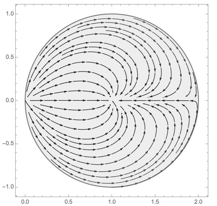
Identifying the hyperbolic plane with the upper half-plane in we consider the space of univalent maps of the form whose image is a Jordan domain. This is subspace of the space of all univalent maps on and it corresponds to the open disk . (See Lemma 4.2.) For each define a Beltrami differential on such
and is zero on the complement of the image of .
This family of Beltrami differentials defines a flow on as follows. For any there is a family of quasiconformal homomeomorphisms whose infinitesimal Beltrami differential at is and there is a smooth path such that . Furthermore the are defined for and the flowline starting at is given by the formula .
The map is a homeomorphism form to the disk in and the flow on induces the flow on the disk. In fact we have the following formula for the flow:
Although these last two paragraphs could be made rigorous as they are not necessary to prove our main result we will not do so. This formula for will follow from our derivation of the limiting vector field in our proof. However, to informally see the connection between this flow and the gradient flow one should view the domains as approximations for a component of the domain discontinuity of a Kleinian group where the imaginary axis is the axis of some short curve in the conformal boundary and the constant is the ratio of the complex length of the curve in the hyperbolic 3-manifold to its length on the boundary. There is an explicit formula for the derivative of this length ratio (see Section 2.1) and in Theorem 4.10 we calculate the limit of this formula as both the length on the boundary and the norm of the Schwarzian approach zero. The limiting formula we find is exactly the formula for the vector field above.
We can also connect the discussion here to our discussion of the flow in the previous section. In our model situation when is near two corresponds to an acylindrical manifold where the surface has small curvature outside of the -thin part where the closer is to two the smaller we can choose . When is near one the corresponds to having small curvature everywhere. While the flow may initially appear to be converging to two it will eventually turn around and head towards one which corresponds being totally geodesic and the hyperbolic manifold .
While our discussion here is only informal we will see that the properties of this limiting model flow play a crucial role in the proof of our main theorem.
2 Weil-Petersson geometry
Let be a closed surface of genus . Then Teichmüller space is the space of marked conformal structures on . Given the cotangent space is the space of holomorphic quadratic differentials on . We let be the the space of Beltrami differentials on . Then there is a pairing between and given by
If we let be the annihilator of under this pairing, we obtain the identification .
Given and then we define the pointwise norm by
where is the hyperbolic metric on . We define the norm of , denoted , to be the norm of the function with respect to the hyperbolic area form on . These norms define Finsler cometrics on the cotangent bundle of and dual Finsler metrics on the tangent bundle of . When this norm comes from an inner product and therefore determines a Riemannian metric on called the Weil-Petersson metric. Classical results are that the Weil-Petersson metric is incomplete (see [Chu, Wol1]) and strictly negatively curved (see [Tro, Wol2]).
In order to describe the Weil-Petersson completion , we first describe the augmented Teichmüller space. For further details on augmented Teichmüller space see [Ab],[Abi] and [Har].
For a compact surface we let be the complex of curves, the simplicial complex organizing the isotopy classes of simple closed curves on that do not represent boundary components. To each isotopy class we associate a vertex , and each -simplex is the span of vertices whose associated isotopy classes can be realized disjointly on .
A point in the augmented Teichmüller space is given by a choice of multicurve , a (-skeleton of a) simplex in , and finite area hyperbolic structures on the complementary subsurfaces . The elements of are the nodes and the point of the completion is a noded Riemann surface. Augmented Teichmüller space is stratified by the simplices of : the collection of noded Riemann surfaces with nodes determined by a given simplex lies in a product of lower-dimensional Teichmüller spaces determined by varying the structures on . This stratum, , inherits a natural metric from the Weil-Petersson metric, which by Masur (see [Mas]) is isometric to the product of Weil-Petersson metrics on the Teichmüller spaces of the complementary subsurfaces.
It follows by Masur also that the augmented Teichmüller space is the Weil-Petersson completion . The completion naturally descends under the action of the mapping class group to a finite diameter metric on the Deligne-Mumford compactification of the moduli space of Riemann surfaces. The strata of the completion can be described as follows;
where is the extended length function of .
2.1 Length functions and Gardiner’s Formula
For an essential closed curve on there are two natural length functions on the deformation space . The first is just the usual length function on Teichmüller space where is the length of the geodesic representative of on the hyperbolic surface . We have used this function already.
The Gardiner formula is a formula for the differential . To state it we identify the universal cover of with the upper half plane normalized so that the imaginary axis is an axis for . Then is an element of the deck group for . We let be the quotient annulus for the action of this element. The annulus also covers so if is a Beltrami differential on (representing a tangent vector in ) then lifts to a Beltrami differential on . The holomorphic quadratic differential on is invariant under the action of so descends to a Beltrami differential on . We will continue to refer to this quadratic differential as on . If we let be the pairing between Beltrami differentials and quadratic differentials on we have
Theorem 2.1 (Gardiner, [Gard])
The derivative of on is given by the formula
If we consider as a closed curve in the hyperbolic 3-manifold then has a complex length. The real part is just the length of the geodesic representative of in while the imaginary part measures the twisting along the geodesic. We need for the imaginary part to be a well defined real number (rather than just a number mod ). For this reason the definition is somewhat involved.
Let be a Kleinian group uniformizing and let be the components of the domain of discontinuity of that cover . The pre-image of in will be a collection of arcs. Fixing an orientation of fixes an orientation of each of the arcs and we can assume that the pre-image contains an oriented arc with initial endpoint and terminal endpoint . Let be the component of the domain of discontinuity that contains and let be a branch of the logarithm defined on . We then define
by
where we are assuming the that is parameterized by arc length. The complex length is independent of the choices we made in its definition.
The complex length is a holomorphic function on and we would also like a formula for its derivative. Miyachi observed ([Miy, First proposition, Section 8]) that the proof of Theorem 2.1 can also be applied to find the derivative of the complex length. As if is a tangent vector in we can also consider it as a tangent vector to at . Then will lift to a -invariant Beltrami differential on . We can extend to be zero everywhere else. The Kleinian group will contain the element . The quotient of the under the action of this element will be a torus and the Beltrami differential will descend to a Beltrami differential on . The quadratic differential will also descend to a quadratic differential on . If is the pairing on we have
Theorem 2.2 (Miyachi, [Miy])
The differential of is given by the formula
For what we will do below it will be useful to decompose this second Gardiner formula into two distinct terms. To describe this decomposition we note that the image of in will be an essential annulus while every other component of will map homeomorphically into (see figure 2). We then write
where has support on the image of and the support of is in the image of the other components of . Then
are the central and auxillary terms of the differential .
It will also be useful to write the central term as a pairing on the annulus . For this let
be the uniformizing map, normalized so that takes the imaginary axis to . Then the pull backs and are both invariant under the isometry and descend to objects on . In fact the Beltrami differential will be the Beltrami differential that we defined above. We can then write the central term as
Note that both the central and auxillary terms only depend on the Beltrami differential . For later convenience we let be the auxillary term. Note that for a Bers slice is the only component of so the auxillary term is always zero. The extra work in the relatively acyndrical case is estimating when is a harmonic Beltrami differential with small -norm.
3 Limits of the flow
As mentioned in the introduction, the flow is the negative of the Weil-Petersson gradient of the renormalized volume function on . The definition of renormalized is somewhat involved and not necessary for our work here. Therefore we will omit it and restrict ourselves to discussing some of its important properties. The first of these is a varitional formula:
This formula implies that our flow is the Weil-Petersson gradient of .
By the Nehari bound on the norm of the Schwarzian derivative of a univalent map (see [Neh]), is bounded with respect to the Teichmüller metric on . Therefore as the Teichmüller metric is complete, the flowlines exists for all time (see [BBB1] for further details).
Also by the gradient description of it follows that along a flowline a
As (see [BBB1]), it follows that
We now describe the further properties of the flow proved in [BBB2] that we will need in our analysis.
Theorem 3.2 (Bridgeman-Brock-Bromberg, [BBB2])
Let be relatively acylidrical and be a flowline for on . Then
- 1.
in the Weil-Petersson completion. Thus is a noded Riemann surface.
- 2.
as .
In order to prove our main theorem, we need to prove that the set of nodes of any limit is empty or alternately that . We will do this by assuming is noded and consider the limits of the projective structure as we zoom in on the nodes. This will produce our limiting model flow which will allow us to obtain a contradiction.
4 Taking limits at a node
The length functions and are smooth functions on if we pair their differentials against the vector field we get a function on . We would like to take the limit of these functions along sequence in where . To do this we will embed in a space of univalent functions. We then use normal families theorems for holomorphic functions to evaluate the limit. We begin by setting up our space.
Let
be the space of quadratic differentials that arise as Schwarzian derivatives of univalent functions from (realized as the upper half plane) to . We give the compact-open topology and recall some basic facts:
- •
is compact.
- •
If and (in the compact-open topology) with then either is constant or is univalent and .
The following result is essentially Montel’s theorem.
Theorem 4.1
Let , and be distinct points in and , and distinct points in . Let be a family of holomorphic maps on that extend continuously to the if they are on the boundary of and assume that for all we have for and while if is not in then is not in . Then is a normal family. If is a limit of a sequence in then for and if is non-constant then for all .
For we say that is -invariant if it is invariant under the isometry (as a quadratic differential). Let be the subspace of quadratic differentials that are -invariant for some . We can define a function
by taking to be the infimum over all positive where is -invariant. Note that if and are -invariant then if we have that is -invariant. This implies that is continuous on . It is possible that and we let . This space will be of particular interest.
Lemma 4.2
If then
with . If let . If let . Then .
Proof: If then is -invariant for a sequence of with . If is -invariant then is -invariant for all . Together this implies that is -invariant for a dense set of so by continuity is -invariant for all . From this invariance we see that if for some then for all . As is holomorphic this implies that .
A direct computation gives that . We’ll show that is univalent exactly when . We can write . Let be the open horizontal strip in between the lines and and let . Then the image of (as the upper half plane) under the map is . The exponential map restricted to is injective exactly when vertical lines in intersect in a segment of length . The intersection of a vertical line with has length where . Thus we have univalence if giving . Completing the square, we get .
The invariance of the quadratic differentials imply invariance for any univalent map with . The next lemma makes this precise.
Lemma 4.3
If the quadratic differential is -invariant and is univalent with then there exists a with . Furthermore is either loxodromic or parabolic and extends continuously to and with the repelling fixed point of and the attracting fixed point if is loxodromic and if is parabolic.
Proof: If is -invariant and is a univalent map with then the map also has Schwarzian . As two maps with the same Schwarzian differ by post-composition of an element of we have that there exists a with . Iterating this formula, for any positive integer we have that . This implies that is -invariant and that the action of on the simply connected space doesn’t have fixed points so must be loxodromic or parabolic. Furthermore the equation implies that extends continuously to and with the repelling fixed point of and the attracting fixed point.
The element is the holonomy of . Let be the subspace of quadratic differentials where and the holonomy is loxodromic. For we define a complex length function as follows. Let be a univalent map with , and . Choose a logarithm, , on . We then define . The expression on the right is independent of the choice of , the choice of and the choice of logarithm.
We also define a function by
Lemma 4.4
The function extends continuously to and for we have
Proof: If is univalent and then we have the Bers’ inequality (or McMullen’s interpretation of the Bers’ inequality, [Mc1, Proposition 6.4]):
| (4.1) |
The statement is usually made in the context of quasifuchsian groups but the proof goes through without change in our setting. From this we see
Thus .
Now assume . Then by Lemma 4.3 we have for some . Take a sequence in with and let and . Since is continuous on we have that and we can choose integers such that . We also fix univalent maps with and the normalization , and . By Theorem 4.1 the will be a normal family. Let be a limit of a subsequence of the . Again by Theorem 4.1, and so the limit won’t be constant which in turn implies that and that is univalent. It follows that . As is the only map with plus the given normalization, any convergent subsequence of the will converge to . Therefore converges to (uniformly on compact sets) without passing to a subsequence.
If is the element of with then the attracting fixed point of and all its powers is . Therefore for some . As lies in a compact set we can pass to a subsequence such that and therefore . Taking the limit of the equation we have
Substituting in for we see that . It follows that is determined by (and hence ). This determines up to a multiple of . However, we also have which implies that so the equation uniquely determines . In particular, before passing to a subsequence.
Let be the the univalent map given by Lemma 4.2 with . Then for some . Note that in with . If then so we must have that and this only occurs when and . If then the repelling and attracting fixed points of are and . This implies that and . It follows that . In both cases we can define and we have that extends continuously to with
We now describe the map from to . It will depend on a choice of essential closed curve on . Given let be a component of the domain of discontinuity that projects to the component of that contains . Let be a uniformizing univalent map that takes the imaginary axis in to an axis for and let . While we have made several choices the quadratic differential is independent of our choices. We can then define by . This map is continuous and . Since is positive on we have that the image of lies in .
Given we define
Thus is the negative of the corresponding harmonic Beltrami differential. We also let be the quotient of under the action and the pair of quadratic differentials and Beltrami differentials on . If is -invariant as a quadratic differential then is -invariant as a Beltrami differential and descends to a Beltrami differential on . We define a function
by
As an immediate consequence of Gardiner’s formula (Theorem 2.1) we have:
Lemma 4.5
Therefore, to study the continuity of we will study the continuity of on .
Lemma 4.6
The function extends continuously to with
for .
Proof: The key to the proof is that if and are -invariant then for all positive integers . Then if for we can choose such that so that
This shows the extends continuously to .
For we have . The pairing is easier to calculate in the strip model for (the region between the horizontal lines and ) with area form . In this model the quadratic differential becomes so and
Taking the real part and multiplying by gives the claimed formula for .
We would like to similarly define a function on for the differential . We will not be able to do this exactly but instead give a formula for the central term. We will need to evaluate the auxillary term separately.
Given let be the univalent map with and and . By Theorem 4.1, this is a normal family. We observe that if is -invariant the quadratic differential is -invariant. We then define a function
by
From Theorem 2.2 and the discussion following it we have:
Lemma 4.7
We now establish the continuity of .
Lemma 4.8
The function extends continuously to with
Proof: The proof is similar to Lemma 4.6. Assume that in converges to and let , , etc. Choose integers with . By Lemma 4.4 the function is continuous and therefore .
Lemma 4.9
Proof: We first assume that . By our normalization so (after possibly passing to a subsequence) as we have where . Since we have that is non-constant and it follows that fixes , and and . This implies that . It follows that
so the lemma holds in the case that .
When (and therefore by Lemma 4.2 ) it will be necessary to choose a different normalization for the so that they don’t converge to a constant function. In particular, similar to the proof of Lemma 4.4 we choose univalent functions with , and and whose Schwarzian is . By Theorem 4.1, the form a normal family. As any limiting function will be non-constant the Schwarzians will also converge to the Schwarzian of the limit. As by assumption we have that any limiting function has Schwarzian . The chosen normalizations of will also persist in the limit. Together these conditions imply that the only possible limiting function is so converges to uniformly on compact sets.
Also, as in Lemma 4.4, we have the equation with . If we choose with then . To calculate we observe that takes the attracting and repelling fixed points of to the attracting and repelling fixed points of . In particular and . It follows that
As this quadratic differential will converge to zero. However, if we multiply the denominator by the denominator will converge to (since ) and the quadratic differential will converge to . We further have that and it follows that if we divide by we have
and since this gives
This proves the lemma when .
We can now prove our limiting formulas for the derivatives of , and .
Theorem 4.10
Let be a relatively acylindrical pair and an essential simple closed curve in . Let be a sequence in with the volume of bounded, , , and for some . Then
- 1.
- 2.
- 3.
In particular if is a flow line for , for a sequence and and then (1)-(3) hold.
Recalling that is a harmonic Beltrami differential, we will derive (2) from Lemmas 4.7 and 4.8 if we can show that . This will be the proven in the next section. In particular, as and we have that . By assumption is bounded and . It then follows from Theorem 5.1 that
and (2) follows.
For the last statement we only need to show that the volume of is bounded. As is a flow line for the gradient of , the negative of renormalized volume, we have that the renormalized volume is bounded. However, the difference between the renormalized volume and convex core volume is bounded by a constant depending only on the the topology of the boundary and the length of the shortest compressible curve (see [BC2, Theorem 1.3]). This last constant is determined by and hence is uniform on . This implies that the convex core volume is bounded and the theorem follows.
5 Bounding the norm of the auxillary term
This section will be dedicated to proving the following theorem:
Theorem 5.1
There exists such that given there exists a such that the following holds. Assume that with . Let be a harmonic Beltrami differential and an essential closed curve on with and . Then
Note that the bound of on is essentially arbitrary. We have chosen it because that is the bound that we get when is the harmonic Beltrami differential associated to the Schwarzian quadratic differential .
Recall that is the pairing of a Beltrami differential and a quadratic differential. The absolute value of the quadratic differential is a Euclidean area form and one can bound the pairing by bounding the norm of the quadratic differential and the area of the quadratic differential. Typically to show that a product of two terms is small one finds a uniform bound on one term and shows that the other term is small. To get the necessary bound here we will need to decompose into two parts. In one the norm will be small while in the other the support will be small while the norm will only be bounded. In particular write as
where the support of is the -thin part of and the support of is the -thick part of . We will then bound and separately.
Most of the work will be to bound so we begin with the easier bound on .
Lemma 5.2
Given there exists an such that if then
Proof: In general bounds on don’t give bounds on . However, a mean value estimate of Teo (see [Teo]) gives bounds for points in the -thick part. In particular there exists a constant such that if then . This implies
The absolute value of the quadratic differential is a Euclidean area form on . If we let be this area we have
and therefore
Letting the lemma follows.
To bound we need to bound the area of the support of . The proof of the following proposition will be most of the work of this section:
Proposition 5.3
There exists such that the following holds. Given there exists a such that if and then
Assuming this for now and we can prove Theorem 5.1.
Proof of Theorem 5.1: By Proposition 5.3 we can fix an such that if and then
Since this implies that
By Proposition 5.2 we can choose such that if then
Note that depends on (and ) but only depends on and . Therefore only depends on and and we can combine the two estimates to get the claimed bound on .
The remainder of this section is dedicated to the proof of Proposition 5.3.
5.1 Margulis tubes
Let be a hyperbolic n-manifold and . Then we define the thick-thin decomposition with
By the Margulis lemma (see [Th1]), there exists a constant such that for then the connected components of are disjoint embedded tubular neighborhoods of cusps or simple geodesics in . These tubes are called Margulis tubes and for a simple closed geodesic, we denote the tube about in by . We further denote the radius of by .
For hyperbolic 3-manifolds, if then by elementary hyperbolic geometry we have,
As has intrinsic Euclidean metric with injectivity radius we have the inequality
In particular
| (5.2) |
We have the following fact due to Brook-Matelski which gives uniform bounds on the change in as varies.
Theorem 5.4 (Brooks-Matelski, [BM])
Given there exists continuous functions such that as and as and for a geodesic in a hyperbolic 3-manifold with then
5.2 Orthogeodesics
Since is a closed surface the components of will be collars of closed geodesics of length . We let be one of these geodesics and the collar. Note that it is possible that . The pre-image of these collars in the domain of discontinuity will be a collection of strips. Under the covering map from to most of these strips will map homeomorphically to strips. The only exception will be that there will be one component in the pre-image of the collar of that will map to an essential annulus in . This exceptional strip will be contained in the central component of . We only need to bound the area of the strips in . We are interested in bounding the area in of those strips that come from auxillary components. To do this we will bound the area of all strips, even those coming from the central component. Our first goal is to bound the area of a single strip. We begin with some preparation.
Associated to is a solid torus cover of . The surface is a component of the conformal boundary of so the -collar of will lie in the conformal boundary of and will lift to a collection of strips in the conformal boundary of . We want to bound the area of these strips in the Euclidean metric on the conformal boundary that comes from taking the absolute value of the quadratic differential . Our bounds will depend on the lengths of and the constant . In the hyperbolic 3-manifold the closed geodesic will lift to a collection of bi-infinite geodesics in and there is a natural correspondence between the strips and these geodesics. We will see that the area of each strip decays exponentially in the distance between and the corresponding lift of .
With this informal discussion in mind we now setup the notation that we will need. Let be the union of and its conformal boundary. Then the cover extends to a cover of . Let
be the covering map. We also have the nearest point projection
to the convex core. This map extends continuously to and lifts to a map
where . In particular we have .
Now let be the collection of strips in that map to . If then this is just the union of components of . If then there is one annular component in that is not included in . By [EMM] the retraction is a -Lipschitz map from the hyperbolic metric on to induced path metric on . Therefore and if is a component of there is a unique component of with (see figure 3).
There is a unique shortest geodesic in from to . This geodesic will be orthogonal to the boundary of the two tubes so we call an orthogeodesic. We will see that the area of decays exponentially in the length of . We note that while it may seem more natural to take the orthogeodesic from the gedoesic to the geodesic in the core of , for our purposes our choice of orthogeodesic is more convenient. We also emphasize that one endpoint of our orthogeodesic will always lie on the boundary of the -Margulis tube while the other end will lie on a lift of the -Margulis tube so while our notation does not emphasize this, the orthogeodesic depends on and as decreases the orthogeodesic will become longer.
If is an embedded half-space in then its closure in the conformal boundary is a round disk . We begin by bounding the area of in terms of the distance between the core geodesic of and .
Lemma 5.5
Let be an isometrically immersed half-space in that is disjoint from the core geodesic with boundary disk . Then
Proof: We can lift the picture to and assume that has endpoints and is the disk of radius centered at with . Note that while the disk is embedded in it may be be immersed in . However, this will only decrease its area. The map sends the geodesic to the geodesic with endpoints and . Thus pulling back the metric we have
Therefore on we have
and it follows that
In the next lemma we show that each component of lies in a round disk in which bounds a half-space in whose distance from the core Margulis tube is given in terms of the length of the associated orthogeodesic.
Lemma 5.6
There exists a such that if and then the following holds. Let and be a component of . Let be the component of with and let be the orthogeodesic between and . Then there is a half-space in whose boundary disk contains with
Proof: By the inequality 5.2 for the radius of the Margulis tube we can choose such that if then
(Choosing will suffice). We also note that the inequality in the statement of the Lemma follows from the lower bound on .
As we assume , it follows that is non-empty so we can consider a component . We again lift the picture to . Let be a lift of to and let be a lift of that is orthogonal to . Further we extend to the perpendicular from to with lift containing . We can assume that is the vertical geodesic segment in the upper-half-space model and that is orthogonal to at . Therefore is the geodesic where . Let be the half-space in that contains and whose boundary plane is orthogonal to at .
The retraction lifts to a retraction
where is the limit set of the Kleinian group uniformizing . Let be the lift of with . Let be the Euclidean disk of radius centered at and the half-space in with boundary . We’ll show that so that if is the image of in then . The immersed half-space bounded by is the image of so we have that is equal to minus the distance from from the boundary plane of to . As this latter distance is this will give
If we can show the inclusion we are done.
We now prove this inclusion. For there is a unique horosphere that intersects in a single point. This point of intersection is . If then will intersect . The perpendicular from to is contained in and therefore must not intersect the interior of . As is the vertical geodesic a simple calculation shows that when the interior of will intersect if . (See Figure 4.) By our choice of , we have . Therefore if we have that and , completing the proof.
Let be the set orthogeodesics from to the components of . With as in the above Lemma 5.6, we have.
Corollary 5.7
Given there exists such that if and then
Proof: We first show that for and then
where is a universal constant.
As then is non-empty. Given a component of let be the component of with and let be the orthogeodesic between and . Then as , by Lemma 5.6, there is an immersed half-space in whose boundary disk contains with
If then . Since the disk contains and by Lemma 5.6 we have we can combine this estimate on with Lemma 5.5 to get
By (5.2) we have
Together the two estimates give
Summing over the set of all orthogeodesics in gives our first estimate.
Now let . We let be the component of that contains and let be the orthogeodesic between and . Note that the map defines an bijection between and . Then is a subsegment of and
where the function on the right comes from Theorem 5.4. Thus for
For the inequality also holds trivially as and as , the righthandside is positive. Thus as as the theorem follows.
5.3 Uniform bounds on the Poincaré series
Except for the last lemma, in this subsection can be any complete hyperbolic 3-manifold uniformized by a Kleinian group .
For we define the Poincaré series
where is the hyperbolic distance. Poincaré series play an important role in dynamics but here we will only be interested in obtaining uniform bounds on which we will then use to bound the similar exponential sum of lengths of orthogeodesics that appears in Corollary 5.7.
We have the following elementary bound.
Lemma 5.8
- •
Let be a closed convex set in and is closure in and let
be the nearest point projection. If and is the ball centered at then contains a round disk that bounds a half-space with
- •
Given and a half-space with boundary disk we have
where is the visual measure on determined by .
Proof: Let be a support plane for at . Then bounds a half-space whose interior is disjoint from the interior of and we let be the round disk in the conformal boundary of this half-space that projects orthogonally to with image in . Let be the point on closest to , a point in , and the orthogonal projection of to . Then forms a planar quadrilateral with one ideal vertex at and right angles at all other vertices. Standard formulas give which can be rewritten in a less symmetric form as . Noting that , and we have so we will be done if we can show that .
For let be the geodesic in from to and let . Note that and since is a contraction (and ) we have that . Let be the ball of radius centered at and let be the closed half-space whose boundary is tangent to at and whose interior is disjoint from . If then is in the interior of and is hence disjoint from . As intersects the boundary plane of we have that , the other endpoint of , will be contained in . As the boundary plane of is orthogonal to , the orthogonal projection of every point in to will have distance from that is at least so we have . Combining inequalities gives when . If then the interior of will be disjoint from as for every we have and by the contraction of . However, if is not contained in it must intersect the interior of . Therefore , and in particular , lie in . As above this implies that completing the proof that .
For the second bullet, as above let be the point on closest to and let be a point in . These three points from a right triangle with one idea angle at and angle at . Therefore is a spherical disk of radius in the visual metric based at . For such right triangles we have . The area of spherical triangle is so . Since and we can combine expressions to get
Using these estimates we can obtain our uniform bound on the Poincaré series.
Lemma 5.9
If is a hyperbolic 3-manifold and a point on the boundary of the convex core with injectivity radius , then for a lift of to we have
Proof: Let be the limit set of and the retract map to the convex hull of the limit set. Let be the ball of radius about . As the injecitivity radius of is we have for all . We define . Since is -invariant we have if . By Lemma 5.8 we have that contains a disk that bounds a half-space with . By the triangle inequality for all we have that . As this gives which in turn implies
where the last sum is bounded by since the disks are all disjoint.
We now can obtain a uniform bound on the exponential sum of orthogeodesic lengths.
Lemma 5.10
Fix and assume that and are closed geodesics in with length . Then the sum
is bounded by a constant that only depends on and the diameter of .
Proof: Choose and let be in the pre-image of under the covering map . We will define a map from to such that where is the diameter of and is at most -to-one. Once we have defined such a we have that
We claim that there exists an integer such that at most components of the pre-image of and in intersect any ball of radius . To see this we note that as has length less than , is non-empty. Thus each point in is contained in a ball of radius which lies inside . Therefore there are disjoint balls of radius in the ball of radius . Thus bounding . Let .
For each we will carefully choose a lift to . More precisely we will carefully choose where the initial endpoint lies and then the terminal endpoint will determine . Note that the endpoints and will lie in the pre-image of so we can choose such that . Then there will be a with and we define and it follows that
The orthogeodesic is determined by which components in the pre-image of and that and lie in. As there are at most in a -neighborhood of and in a -neighborhood of there are at most orthogeodesics with so is at most -to-one.
For the previous lemma to be useful need to able to control the diameter of . The following argument is well known.
Lemma 5.11
Let and a geometrically finite hyperbolic manifold and convex core volume less than . Then the diameter of every connected component of , the -thick part of the convex core, is bounded by a constant that is a function of and length of the shortest compressible curve in .
Proof: Given in connected component of let be a path joining . Then is continuous with and and we can take with for where . Then the balls are disjoint, embedded and contained in . Thus the number of disjoint -balls is bounded in terms of the volume of which in turn bounds .
To bound the volume of , let be the volume of , then the area of . If is the bending lamination on then an easy calculation gives
where is the length of . Also by [BBB1], there are universal constants such that . Integrating, it follows that the volume of is bounded by a function of , and .
To apply the previous lemma to bound the diameter of we need to know that this set is connected. In general this will be false. The next lemma show that in our setting it holds for sufficiently small for hyperbolic manifolds in a relatively acylindrical deformation space.
Lemma 5.12
Given with relatively acylindrical then there exists a such that if then is connected.
Proof: Let be the union of components of that face . The retraction from to is Lipschitz with Lipschitz constant only depending on (see [BC1]). Therefore the diameter of is bounded by , a constant depending only on and .
Let be the union of components of facing and recall that the path metric on is hyperbolic. Since is relatively acylindrical there is at most one homotopy class of curve in that is homotopic to . If there is such a curve, let be the -Margulis collar about its geodesic representative in . Note that if there is no such curve or the curve has length then is empty. By a theorem of Bers has a bounded length pants decomposition with constants only depending on the topology of and each point in the -thick part of is a uniformly bounded distance from at least two of these curves. On the other hand if is in the -thin part but not in there is an essential curve of length that is not homotopic to a multiple of . Therefore there exists an such that for there is a closed curve of length containing which is not homotopic to a multiple of .
We now choose such that . Let be a point in . If then the diameter bound on implies that . This is a contradiction since cannot be contained in a Margulis tube. If then there is an essential closed curve through of length that is not homotopic to . Then the length bound implies that which is again a contradiction. It follows that .
To finish the proof we show that is connected. We can assume that and are transverse. (If not we can slightly decrease .) On the intersection will be a collection of simple closed curves that are either homotopic to or are contractible and bound disks. These curves will bound the region of that is contained in . We’ll show that it is either a pair of parallel curves homotopic to or a collection of contractible curves bounding disks whose interiors are disjoint from .
First we assume that the intersection of with the bending lamination is zero. Then the collar is totally geodesic outside of where it is bent at some angle (possibly zero). This implies that for points in the injectivity radius on agrees with the injectivity radius in the ambient hyperbolic 3-manifold and therefore the intersection of with is the -Margulis collar about . In particular is a pair of parallel curves and is an annulus bounded by these curves and therefore is connected. If intersects the bending lamination then we can foliate with geodesic segments in joining the boundary components of . Note that is contained in and as any geodesic in will intersect in a connected set we have that each geodesic arc of the foliation has connected intersection with . Thus the intersection is either empty, a point or a closed interval. By continuity of the foliation this implies that is either a union of disks or an annulus. In the annulus case, then is also an annulus and therefore is connected. For the disk case, intersects in a union of disjoint disks and is either a union of disks or the complement of a union of disks. As is the intersection of two convex sets, it is connected. Therefore must be the complement of a union of disks and therefore is connected.
5.4 Proof of Proposition 5.3
We now are ready to prove Proposition 5.3 which will complete the proof that the auxillary components do not contribute to the limiting model flow. We restate it.
Proposition 5.3 There exists such that the following holds. Given there exists a such that if and then
Proof: The support of is contained in the union of where ranges over the closed geodesics of length in . There are at most such curves, where is the genus of , so it will be enough to bound the area of the individual .
Fix as in Lemma 5.12 and choose that maps to under the covering map . Then by Lemmas 5.9 and 5.10 we have for of length less than
where is a the diameter bound on and depends on . By Lemma 5.11, the diameter of each component of is bounded by a constant only depending on the the volume of . By Lemma 5.12, is connected. Therefore , and hence , only depend on the volume of and the sum only depends on the volume of . The result then follows from Corollary 5.7 by further choosing so that .
6 Vector field at infinity
We now return to our flow line of the gradient vector field on and recall that by Theorem 3.2 we have and . The surface is a noded surface (with possibly empty nodal set). We can assume that is one of the nodes and let Then by Theorem 4.10 if is a subsequence with for some we have where is the vector field

Proposition 6.1
The critical points of the vector field are (unstable), (stable), (saddle), and (saddle). The basin of attraction of is the disk and the circle consists of two trajectories from to .
Proof: A direct computation shows that and that there are no other zeros. The linearization of each zero is non-trivial and gives that each zero of is as described. Once we show that the circle consists of two trajectories from to it will follow that is the basin of attraction for as there are exactly two trajectories limiting to the unstable fixed point at and therefore all the other trajectories in the disk must limit to (since they can’t limit to the unstable fixed point at ).
If we let be the radial vector field centered at then the Euclidean inner product of and is given by taking the real part of the product of and the conjugate of (as functions). Points in the circle are of the form and on calculates to see that for such points so is tangent to this circle.
On the other hand if we let be the constant horizontal vector field then on the circle we have
| (6.3) |
This is zero only when is or (and is or ) and is positive otherwise. This implies that and are the only critical points on the circle and that the flows lines are from to as claimed.
We will use the next lemma to analyze the limiting behaviour of the path .
Lemma 6.2
Let be a smooth vector field on and be a smooth path whose image lies in a compact subset. Also assume that for all sequences with converging to some then .
Let be the accumulation set for . Then is a union of trajectories of the flow of .
If contains distinct points and then there exists an such that if there is a trajectory and a such that and and similarly a trajectory with . In particular if is an attracting or repelling fixed point of or is an isolated point of then and .
Proof: Since the image of has compact support we can assume that has compact support and is bounded. We first show that as . If not we can find a sequence such that in but converges to some non-zero . But, by assumption which implies , a contradiction.
Therefore is bounded. Now let and for choose a sequence with . As the are also bounded, by Arzela-Ascoli (after possibly passing to a subsequence), we have a locally uniform limit and limits locally uniformly to . Note that is defined on all of . Therefore we have
which implies that is a trajectory of . Note that the image of will be contained in so we have shown that is a union of trajectories.
For the final statement let . Then for any the path must leave and enter any ball of radius centered at infinitely often. Therefore we can find such that and . After possibly passing to a subsequence there is a trajectory with and . Continuity implies that and as claimed. The other inequality follows similarly.
We can now show that converges to one.
Proposition 6.3
As we have .
Proof: Let be the accumulation set of . As is contained in the disk then we must have all of the trajectories in are contained in this disk. Note that any non-constant trajectory in the disk contains either or (and often both) in its closure so if contains a non-constant trajectory then it contains either or and by the second part of Lemma 6.2 we then have or . In particular, cannot contain any non-constant trajectories and therefore, again by the second part of Lemma 6.2, must be equal to one of the zeros of in the disk . We finish the proof by showing that does not converge to or .
If as we have , then for we have . But by Theorem 4.10
As it follows that is increasing for contradicting thats . Thus .
If as then by (1) of Theorem 4.10 we have
for all sequences . On the other hand, as as , we can choose a subsequence such that and therefore
This is a contradiction and therefore . It follows that .
7 Main Theorem
Before we finish the proof of the main theorem, we will need to following bound on the -norm of a harmonic Beltrami differential in terms of the -norm and the derivative of the length of short geodesics.
Lemma 7.1 (Wolpert, [Wol3, Lemma 11])
There exists an satisfying the following. Given there exists such that if is the family of geodesics with for and is a harmonic Beltrami differential on then
where is the component of orthogonal (in the Weil-Petersson inner product) to the span of the of the gradients .
Wolpert’s original bound is in terms of the gradient of the root-length functions . One can translate his statement to the above statement via the chain rule.
The above gives the following immediate corollary;
Corollary 7.2
Let be relatively acylindrical and be a flowline for , with quadratic differential . Then
Proof: We have where is the collection of nodes. Then there is an such that if then . We apply the above to for . As we have
By Lemma 6.3 . Thus by Lemma 4.10
Thus as the result follows.
We now have everything in place to prove our main result.
Theorem 1.1
Let be relatively acylindrical and be a flowline for , then converges to
Proof: If is the corresponding flowline of on we have that . We let be the quadratic differential given by the Schwarzian on . Then by Theorem 3.2 we have that where is a possibly noded surface in the Weil-Petersson completion . We will show that the set of nodes is empty at the is actually contained in .
We let be the restriction of the skinning map to .
By McMullen, the skinning map is contracting in the Teichmuller metric with contraction factor depending only on the topology of (see [Mc1, Theorem 6,1, Corollary 6.2]). It follows that there is a unique fixed point of which we label since .
For any contraction mapping we can bound the distance from a point to the fixed point in terms of the distance between the point and its first iterate. In particular for any we have
By the Ahlfors-Weill quasiconformal reflection theorem (see [AW, Theorem A]) if then
By Corollary 7.2 above so we can combine the two inequalities to get . Therefore as claimed.
References
- [Ab] W. Abikoff. Degenerating families of Riemann surfaces. Annals of Math. 105(1977), 29–44.
- [Abi] W. Abikoff. The Real Analytic Theory of Teichmüller Space. Lecture notes in mathematics. Springer-Verlag, 1980.
- [AW] L. Ahlfors and G. Weill. A uniqueness theorem for Beltrami equations. Proc. Amer. Math. Soc. 13(1962), 975–978.
- [BBB1] M. Bridgeman, J. Brock, and K. Bromberg. Schwarzian derivatives, projective structures, and the Weil-Petersson gradient flow for renormalized volume. Duke Math Journal 168(April 2019), 867–896.
- [BBB2] M. Bridgeman, J. Brock, and K. Bromberg. The Weil-Petersson gradient flow of renormalized volume and 3-dimensional convex cores. Geometry and Topology (accepted 2022).
- [BC1] M. Bridgeman and R.D. Canary. From the boundary of the convex core to the conformal boundary. Geometrica Dedicata, 96(2003).
- [BC2] M. Bridgeman and R.D. Canary. Renormalized volume and volume of the convex core. Annales de l’Institut Fourier (to appear 2017).
- [BM] R. Brooks and J. P. Matelski. Collars for Kleinian Groups. Duke Math. J. 49(1982), 163–182.
- [Chu] Tienchen Chu. The Weil-Petersson metric in the moduli space. Chinese J. Math. 4(1976), 29–51.
- [Dum1] David Dumas. Bers slices and related galleries, https://www.dumas.io/slices/.
- [Dum2] David Dumas. Github of programs for computing Bers slices, https://github.com/daviddumas/cp1.
- [Ep] C. L. Epstein. Envelopes of horospheres and Weingarten surfaces in hyperbolic 3-space. preprint.
- [EMM] D. B. A. Epstein, A. Marden, and V. Markovic. Quasiconformal homeomorphisms and the convex hull boundary. Ann. of Math. (2) 159(2004), 305–336.
- [Gard] F. Gardiner. Schiffer’s interior variation and quasiconformal mapping. Duke J. Math. 42(1975), 371–380.
- [GW] C.R. Graham and E. Witten. Conformal anomaly of submanifold observables in AdS/CFT correspondence. Nucl. Phys. B 546(1999), 52–64.
- [Har] W. J. Harvey. Spaces of discrete groups. In Discrete Groups and Automorphic Functions, pages 295–348. Academic Press, 1977.
- [KSWY] Yohei Komori, Toshiyuki Sugawa, Masaaki Wada, and Yasushi Yamashita. Drawing Bers Embeddings of the Teichmüller Space of Once-Punctured Tori. Experiment. Math. 15(2006), 51–60.
- [Kra] I. Kra. Deformation spaces. In A Crash Course on Kleinian Groups, pages 48–70. Springer-Verlag Lecture Notes in Math. 400, 1974.
- [KS1] K. Krasnov and J-M. Schlenker. On the renomalized volume of hyperbolic 3-manifolds. Comm. Math. Phys. 279(2008), 637–668.
- [KS2] K. Krasnov and J-M. Schlenker. The Weil-Petersson metric and the renormalized volume of hyperbolic 3-manifolds. Handbook of Teichmuller theory III(2012), 779–819.
- [Mas] H. Masur. The extension of the Weil-Petersson metric to the boundary of Teichmüller space. Duke Math. J. 43(1976), 623–635.
- [Mc1] C. McMullen. Iteration on Teichmüller space. Invent. math. 99(1990), 425–454.
- [Mc2] C. McMullen. Cusps are dense. Annals of Math. 133(1991), 217–247.
- [Miy] Hideki Miyachi. Cusps in complex boundaries of one-dimensional Teichmüller space. Conform. Geom. Dyn. 7(2003), 103–151.
- [Mor] Sergiu Moroianu. Convexity of the renormalized volume of hyperbolic 3-manifolds. Amer. J. Math. 139(2017), 1379–1394.
- [Neh] Z. Nehari. Schwarzian derivatives and schlicht functions. Bull. AMS 55(1949), 545–551.
- [Sto] P. Storm. Hyperbolic convex cores and simplicial volume. Duke Mathematical Journal 140, (2)(2007), 281–319.
- [TL] L. Takhtajan and L.Teo. Liouville action and Weil-Petersson metric on deformation spaces, global Kleinian reciprocity and holography. Comm. Math. Phys. 239(2003), 183–240.
- [Teo] L. P. Teo. The Weil-Petersson geometry of the moduli space of Riemann surfaces. Proc. Amer. Math. Soc 137(2009), 541–552.
- [Th1] W. P. Thurston. Geometry and Topology of Three-Manifolds. Princeton lecture notes, 1979.
- [Th2] W. P. Thurston. Hyperbolic structures on 3-manifolds I: Deformations of acylindrical manifolds. Annals of Math. 124(1986), 203–246.
- [Tro] A. J. Tromba. On a natural algebraic affine connection on the space of almost complex structures and the curvature of Teichmüller space with respect to its Weil-Petersson metric. Manuscripta Math. 56(1986), 475–497.
- [VP] Franco Vargas Pallete. Local convexity of renormalized volume for rank-1 cusped manifolds. Math. Res. Lett. 26(2019), 903–919.
- [Wol1] S. Wolpert. Noncompleteness of the Weil-Petersson metric for Teichmüller space. Pacific J. Math. 61(1975), 573–577.
- [Wol2] S. Wolpert. Chern forms and the Riemann tensor for the moduli space of curves. Invent. Math. 85(1986), 119–145.
- [Wol3] S. Wolpert. Equiboundedness of the Weil-Petersson metric. Transactions of the American Mathematical Society 369(2017), 5871–5887.
- [ZT] P. G. Zograf and L. A. Takhtadzhyan. On the uniformization of Riemann surfaces and on the Weil-Petersson metric on the Teichmüller and Schottky spaces. Mat. Sb. (N.S.) 132(174)(1987), 304–321, 444.