Quasiparticle interference patterns in bilayer graphene with trigonal warping

Vardan Kaladzhyan Email: vardan.kaladzhyan@phystech.edu Affiliation: Department of Physics, University of Basel, Klingelbergstrasse 82, CH-4056 Basel, Switzerland Frédéric Joucken Affiliation: Department of Physics, University of California, Santa Cruz, California, USA Zhehao Ge Affiliation: Department of Physics, University of California, Santa Cruz, California, USA Eberth A. Quezada-Lopez Affiliation: Department of Physics, University of California, Santa Cruz, California, USA Takashi Taniguchi Affiliation: International Center for Materials Nanoarchitectonics, National Institute for Materials Science, 1-1 Namiki, Tsukuba 305-0044, Japan Kenji Watanabe Affiliation: Research Center for Functional Materials, National Institute for Materials Science, 1-1 Namiki, Tsukuba 305-0044, Japan Jairo Velasco Jr Affiliation: Department of Physics, University of California, Santa Cruz, California, USA Cristina Bena Affiliation: Institut de Physique Théorique, Université Paris Saclay, CEA CNRS, Orme des Merisiers, 91190 Gif-sur-Yvette Cedex, France

August 11, 2026

Abstract

We calculate the form of quasiparticle interference patterns in bilayer graphene within a low-energy description, taking into account perturbatively the trigonal warping terms. We introduce four different types of impurities localized on the A and B sublattices of the first and the second layer, and we obtain closed-form analytical expressions both in real and Fourier spaces for the oscillatory corrections to the local density of states generated by the impurities. Finally, we compare our findings with recent experimental and semi-analytical T-matrix results from arXiv:2104.10620 and we show that there is a very good agreement between our findings and the previous results, as well as with the experimental data.

I Introduction

In realistic materials impurities and defects are ubiquitous players that often hinder the interpretation of experimental results. However, certain manifestations of their presence can be useful to reveal some interesting properties and to access the parameters of the underlying systems. For instance, Friedel oscillations in the local density of states Friedel 1958, often referred to as “quasiparticle interference patterns”, allow to extract the Fermi momentum of the electrons, as well as to infer about the dimension of the system under consideration. These oscillations arise as a result of impurity scattering processes and represent interferences between incoming and outgoing wave packets.

Quasiparticle interference patterns have been extensively studied, both theoretically and experimentally, in graphene, be it single layer or multi-layer Cheianov and Fal’ko 2006; Mariani et al. 2007; Kivelson et al. 2003; Bena and Kivelson 2005; Bena 2008; Bena 2009; Wehling et al. 2007; Peres et al. 2006; Peres et al. 2007; Vozmediano et al. 2005; Ando 2006; Pogorelov 2006; Skrypnyk and Loktev 2006; Skrypnyk and Loktev 2007; Katsnelson and Geim 2007; Dutreix and Katsnelson 2016. For instance, it was shown that in a single-layer graphene sheet the correction to the local density of states in the presence of impurities decays as $1/r^{2}$ Cheianov and Fal’ko 2006; Mariani et al. 2007; Bena 2008; Bena 2009 versus the expected $1/r$ behavior prevalent in two-dimensional systems Bena and Kivelson 2005; Bena 2008. However, as it was demonstrated in Ref. [Bena 2008], the $1/r$ decay is restored in bilayer graphene. Experimentally quasiparticle interference patterns are accessible via Fourier-transform scanning tunneling microscopy Mallet et al. 2007; Mallet et al. 2016.

It was anticipated theoretically Charlier et al. 1991; McCann and Fal’ko 2006; McCann and Koshino 2013 and confirmed experimentally Kuzmenko et al. 2009; Joucken et al. 2020; Zibrov et al. 2018; Varlet et al. 2014; Orlita et al. 2012; Shi et al. 2018 that there is a threefold symmetric warping of the bands in bilayer graphene, the so-called “trigonal warping”. Originating from the interlayer coupling between non-dimer orbitals A1 and B2, the latter splits the Dirac points inherent in graphene-like systems into four Dirac points, as it is shown in Fig. 1 for one of the valleys. Furthermore, as it was demonstrated in Refs. [Charlier et al. 1991; McCann and Koshino 2013; Kechedzhi et al. 2007; Zibrov et al. 2018; Varlet et al. 2014; Orlita et al. 2012; Shi et al. 2018; Ge et al. 2020], the trigonal warping can have important consequences on the physical properties of graphitic systems. It is worth noting that the effect of the trigonal warping observable in experiments is stronger as one approaches the Dirac points. Finally, note that some confusion regarding the orientation of the trigonal warping has been solved both theoretically Jung and MacDonald 2014 and experimentally Joucken et al. 2020.

Refer to caption — Figure 1: Equal-energy contours for bilayer graphene in the absence and in the presence of trigonal warping (left and right panels, respectively). The corresponding band structures are shown as insets.

In this paper we calculate analytically the quasiparticle interference patterns in bilayer graphene taking into account the trigonal warping terms. Using a first-order perturbative expansion in trigonal warping, and the $T$ -matrix formalism Byers et al. 1993; Salkola et al. 1996; Ziegler et al. 1996; Mahan 2000; Balatsky et al. 2006; Bena 2016, we find closed analytical expressions for the correction to the local density of states introduced by four distinct types of impurities localized at different sublattices and layers of the bilayer graphene. Our most interesting observations are that at the energies close to the Dirac points the real-space oscillations reflect the symmetry of the trigonal warping, and most saliently, one can extract in a closed analytical form the values of momenta at which the oscillations occur. By analyzing our findings both in the real and Fourier space, we provide a comparison with recent experiments and semi-analytical calculations Joucken et al. 2020; Joucken et al. 2021, and we show that our results are in good agreement with the experimental observations.

We proceed as follows: in Sec. II we derive the low-energy description of bilayer graphene, in Sec. III we calculate perturbatively the bare retarded Green’s function of the system in the real and Fourier space. In Sec. IV we apply the $T$ -matrix formalism to compute the quasiparticle interference patterns and compare these findings to the experimental results, leaving the conclusions to Sec. V.

II Low-energy description

We start by writing down the simplest lattice model for bilayer graphene McCann and Koshino 2013; Joucken et al. 2020. In the basis $\left\{\psi_{\bm{k}}^{A1},\,\psi_{\bm{k}}^{B1},\,\psi_{\bm{k}}^{A2},\,\psi_{\bm{k}}^{B2}\right\}$ , where $A,B$ and $1,2$ refer to sublattices and layers, respectively, we have:

\displaystyle H(\bm{k})\equiv\begin{pmatrix}0&-\gamma_{0}f(\bm{k})&0&-\gamma_{3}f^{*}(\bm{k})\\ -\gamma_{0}f^{*}(\bm{k})&0&\gamma_{1}&0\\ 0&\gamma_{1}&0&-\gamma_{0}f(\bm{k})\\ -\gamma_{3}f(\bm{k})&0&-\gamma_{0}f^{*}(\bm{k})&0\end{pmatrix},

(1)

where we defined $f(\bm{k})\equiv e^{ik_{y}a/\sqrt{3}}+2e^{-ik_{y}a/2\sqrt{3}}\cos\frac{k_{x}a}{2}$ , $a=2.46$ Å is the lattice constant, the intra- and interlayer hopping constants are denoted by $\gamma_{0}=3.3\,$ eV and $\gamma_{1}=0.42\,$ eV, respectively, and the trigonal warping parameter $\gamma_{3}=-0.3\,$ eV. The sign of the latter stands for the warping orientation.

To derive a low-energy theory we expand the Hamiltonian in Eq. (1) around $K_{s}\equiv\left(s\frac{4\pi}{3a},0\right)$ points, where $s=\pm$ is the valley index, and we get:

\displaystyle f(\bm{k})\approx-\frac{\sqrt{3}}{2}(sk_{x}-ik_{y})a

(2)

To simplify further the calculations, we divide the Hamiltonian above by $\gamma_{0}\sqrt{3}/2$ , thereby rendering it dimensionless, and we introduce $\bm{q}\equiv\bm{k}a$ :

\displaystyle\mathcal{H}(\bm{q})=\begin{pmatrix}0&sqe^{-is\phi_{q}}&0&\gamma_{03}sqe^{+is\phi_{q}}\\ sqe^{+is\phi_{q}}&0&\gamma_{01}&0\\ 0&\gamma_{01}&0&sqe^{-is\phi_{q}}\\ \gamma_{03}sqe^{-is\phi_{q}}&0&sqe^{+is\phi_{q}}&0\end{pmatrix},

(3)

where

\displaystyle\mathcal{H}\equiv\frac{2H}{\gamma_{0}\sqrt{3}},\;\gamma_{01}=\frac{2\gamma_{1}}{\gamma_{0}\sqrt{3}}\approx 0.15,\;\gamma_{03}=\frac{\gamma_{3}}{\gamma_{0}}\approx-0.09.

(4)

For the sake of simplicity, above we introduced polar coordinates in momentum space, i.e., we replaced $\bm{q}=(q_{x},\,q_{y})\to(q,\,\phi_{q})$ , where $q=\sqrt{q_{x}^{2}+q_{y}^{2}}\geqslant 0$ , and $\phi_{q}\in\left[0,\,2\pi\right)$ with $e^{\pm is\phi_{q}}=\frac{q_{x}\pm isq_{y}}{q}$ .

The Hamiltonian in Eq. (3) provides a low-energy description for bilayer graphene with trigonal warping.

III Perturbative calculation of the retarded Green’s function

In what follows we calculate the bare retarded Green’s function in momentum space and in real space. The former is easily feasible, however, the latter requires a very complicated Fourier transform. Therefore, below we adopt a different strategy and we resort to a perturbative approach for both the momentum-space and real-space calculations.

III.1 Momentum space

We rewrite the Hamiltonian in Eq. (3) as a sum of $\mathcal{H}_{0}(\bm{q})$ , which is unperturbed by trigonal warping, and $\mathcal{V}(\bm{q})$ , embodying the trigonal warping:

	$\displaystyle\mathcal{H}(\bm{q})=$	$\displaystyle\underbrace{\begin{pmatrix}0&sqe^{-is\phi_{q}}&0&0\\ sqe^{+is\phi_{q}}&0&\gamma_{01}&0\\ 0&\gamma_{01}&0&sqe^{-is\phi_{q}}\\ 0&0&sqe^{+is\phi_{q}}&0\end{pmatrix}}_{\mathcal{H}_{0}(\bm{q})}+$
		$\displaystyle\underbrace{\begin{pmatrix}0&0&0&\gamma_{03}sqe^{+is\phi_{q}}\\ 0&0&0&0\\ 0&0&0&0\\ \gamma_{03}sqe^{-is\phi_{q}}&0&0&0\end{pmatrix}}_{\mathcal{V}(\bm{q})}.$		(5)

Below we calculate the Matsubara Green’s function $G(i\omega,\bm{q})\equiv\left[i\omega-\mathcal{H}(\bm{q})\right]^{-1}$ , and then perform an analytic continuation replacing $i\omega\to\epsilon+i0^{+}$ to recover the retarded Green’s function $\mathcal{G}(\epsilon,\bm{q})$ .

A first-order perturbation theory in $\gamma_{03}$ yields:

	$\displaystyle G(i\omega_{n},\bm{q})=\left[i\omega-\mathcal{H}_{0}(\bm{q})-\mathcal{V}(\bm{q})\right]^{-1}=\phantom{aaaaaaaaaaaa}$
	$\displaystyle=\left[G^{-1}_{0}(i\omega,\bm{q})-\mathcal{V}(\bm{q})\right]^{-1}\approx G_{0}(i\omega,\bm{q})+G_{1}(i\omega,\bm{q}),$

where $G_{1}(i\omega,\bm{q})\equiv G_{0}(i\omega,\bm{q})\mathcal{V}(\bm{q})G_{0}(i\omega,\bm{q})$ is the first-order correction in $\gamma_{03}$ . Finally, in momentum space we have:

\displaystyle G_{0}(i\omega,\bm{q})=\frac{1}{D_{q}}\begin{pmatrix}g_{0}^{11}&\left(g_{0}^{21}\right)^{\star}&\left(g_{0}^{31}\right)^{\star}&\left(g_{0}^{41}\right)^{\star}\\ g_{0}^{21}&g_{0}^{22}&g_{0}^{32}&\left(g_{0}^{31}\right)^{\star}\\ g_{0}^{31}&g_{0}^{32}&g_{0}^{22}&\left(g_{0}^{21}\right)^{\star}\\ g_{0}^{41}&g_{0}^{31}&g_{0}^{21}&g_{0}^{11}\end{pmatrix}.

(6)

Here $D_{q}\equiv(q^{2}-(i\omega)^{2}+i\omega\gamma_{01})(q^{2}-(i\omega)^{2}-i\omega\gamma_{01})$ , while $g_{0}^{ij}$ denotes the $(ij)$ -th element of the matrix $g_{0}$ , with

		$\displaystyle g_{0}^{11}\equiv i\omega((i\omega)^{2}-\gamma_{01}^{2})-i\omega q^{2},\;\;g_{0}^{22}\equiv(i\omega)^{3}-(i\omega)q^{2},$
		$\displaystyle g_{0}^{21}\equiv(i\omega)^{2}\cdot sqe^{is\phi_{q}}-sq^{3}e^{is\phi_{q}},\;\;g_{0}^{31}\equiv i\omega\gamma_{01}\cdot sqe^{is\phi_{q}},$
		$\displaystyle g_{0}^{32}\equiv(i\omega)^{2}\gamma_{01},\;\;g_{0}^{41}\equiv\gamma_{01}\cdot q^{2}e^{2is\phi_{q}}.$		(7)

We use the $\star$ symbol to denote replacing $\phi_{q}\to-\phi_{q}$ , e.g., $\left(g_{0}^{31}\right)^{\star}=i\omega\gamma_{01}\cdot sqe^{-is\phi_{q}}$ .

The first-order correction in trigonal warping is given by

\displaystyle G_{1}(i\omega,\bm{q})=\frac{\gamma_{03}}{D_{q}^{2}}\begin{pmatrix}g_{1}^{11}&\left(g_{1}^{21}\right)^{\star}&\left(g_{1}^{31}\right)^{\star}&\left(g_{1}^{41}\right)^{\star}\\ g_{1}^{21}&g_{1}^{22}&\left(g_{1}^{32}\right)^{\star}&\left(g_{1}^{31}\right)^{\star}\\ g_{1}^{31}&g_{1}^{32}&g_{1}^{22}&\left(g_{1}^{21}\right)^{\star}\\ g_{1}^{41}&g_{1}^{31}&g_{1}^{21}&g_{1}^{11}\end{pmatrix},

(8)

where $g_{1}^{ij}$ are defined in Appendix A.2.

III.2 Bare retarded Green’s function in real space

In this subsection we calculate the Fourier transform of the Matsubara Green’s function obtained perurbatively in the previous section. For this we need to calculate the two following integrals:

	$\displaystyle G(i\omega,\bm{r})$	$\displaystyle=\underbrace{\int\limits_{0}^{+\infty}\frac{qdq}{2\pi}\int\limits_{0}^{2\pi}\frac{d\phi_{q}}{2\pi}G_{0}(i\omega,\bm{q})e^{iqr\cos(\phi_{q}-\phi_{r})}}_{G_{0}(i\omega,\bm{r})}+$
		$\displaystyle\underbrace{\int\limits_{0}^{+\infty}\frac{qdq}{2\pi}\int\limits_{0}^{2\pi}\frac{d\phi_{q}}{2\pi}G_{1}(i\omega,\bm{q})e^{iqr\cos(\phi_{q}-\phi_{r})}}_{G_{1}(i\omega,\bm{r})}.$		(9)

Above we introduced polar coordinates in real space, as well as in momentum space, i.e., $\bm{r}=(x,\,y)\to(r,\,\phi_{r})$ , where $r\geqslant 0$ and $\phi_{r}\in\left[0,\,2\pi\right)$ . For the sake of brevity, we leave the final real-space form of the Green’s functions, as well as the lengthy integral calculations to Appendixes B.1 and B.2.

IV Quasiparticle Interference Patterns

In what follows we introduce localized delta-function impurities into the system and we calculate the associated quasiparticle interference patterns via the $T$ -matrix formalism. To simplify the derivation we assume that impurities are localised on a specific sublattice and in a specific layer, and we define their amplitudes as

	$\displaystyle V_{A1}$	$\displaystyle=U\begin{pmatrix}1&0&0&0\\ 0&0&0&0\\ 0&0&0&0\\ 0&0&0&0\end{pmatrix}\negthickspace,\,\;V_{B1}=U\begin{pmatrix}0&0&0&0\\ 0&1&0&0\\ 0&0&0&0\\ 0&0&0&0\end{pmatrix}\negthickspace,$
	$\displaystyle V_{A2}$	$\displaystyle=U\begin{pmatrix}0&0&0&0\\ 0&0&0&0\\ 0&0&1&0\\ 0&0&0&0\end{pmatrix}\negthickspace,\,\;V_{B2}=U\begin{pmatrix}0&0&0&0\\ 0&0&0&0\\ 0&0&0&0\\ 0&0&0&1\end{pmatrix}\negthickspace,$		(10)

where $U$ denotes the magnitude of the impurity potential. Below we proceed in two steps: first, with the help of the real-space form of the Green’s function defined in Eqs. (9), (39) and (45-52), we compute the $T$ -matrix that accounts for all-order impurity scattering processes. Second, we find the correction to the local density of states in the presence of impurities.

IV.1 $T$ -matrix

To find the $T$ -matrix we need to evaluate the following expression Byers et al. 1993; Salkola et al. 1996; Ziegler et al. 1996; Mahan 2000; Balatsky et al. 2006; Bena 2016:

\displaystyle T(i\omega)=\left[\mathbb{I}-V\cdot\lim\limits_{\bm{r}\to\bm{0}}G(i\omega,\bm{r})\right]^{-1}V,

(11)

where $G(i\omega,\bm{r})\equiv G_{0}(i\omega,\bm{r})+G_{1}(i\omega,\bm{r})$ , and $V=V_{A1}$ , $V_{B1}$ , $V_{A2}$ , $V_{B2}$ , depending on the chosen impurity type. The first-order correction to the Green’s function does not contribute to the $T$ -matrix, since $\lim\limits_{\bm{r}\to\bm{0}}G_{1}(i\omega,\bm{r})=0$ due to the angular parts. Thus, the corresponding T-matrices are given by:

	$\displaystyle T_{A1}$	$\displaystyle=\begin{pmatrix}f(i\omega)&0&0&0\\ 0&0&0&0\\ 0&0&0&0\\ 0&0&0&0\end{pmatrix}\negthickspace,\,T_{B1}=\begin{pmatrix}0&0&0&0\\ 0&g(i\omega)&0&0\\ 0&0&0&0\\ 0&0&0&0\end{pmatrix}\negthickspace,$
	$\displaystyle T_{A2}$	$\displaystyle=\begin{pmatrix}0&0&0&0\\ 0&0&0&0\\ 0&0&g(i\omega)&0\\ 0&0&0&0\end{pmatrix}\negthickspace,\,T_{B2}=\begin{pmatrix}0&0&0&0\\ 0&0&0&0\\ 0&0&0&0\\ 0&0&0&f(i\omega)\end{pmatrix}\negthickspace,$		(12)

where we defined

	$\displaystyle f(i\omega)$	$\displaystyle\equiv\frac{U}{1-U\lim\limits_{\bm{r}\to\bm{0}}\left[i\omega((i\omega)^{2}-\gamma_{01}^{2})I_{00}-i\omega I_{03}\right]},$		(13)
	$\displaystyle g(i\omega)$	$\displaystyle\equiv\frac{U}{1-U\lim\limits_{\bm{r}\to\bm{0}}\left[(i\omega)^{3}I_{00}-i\omega I_{03}\right]}.$		(14)

We leave the calculation of the limits in Eqs. (13) and (14) to Appendix C, and we present the final result here:

	$\displaystyle\lim\limits_{\bm{r}\to\bm{0}}I_{00}$	$\displaystyle=\frac{1}{4\pi\gamma_{01}i\omega}\left(\Omega_{+}-\Omega_{-}\right),$		(15)
	$\displaystyle\lim\limits_{\bm{r}\to\bm{0}}I_{03}$	$\displaystyle=-\frac{1}{4\pi\gamma_{01}i\omega}\sum\limits_{\sigma=\pm}\sigma\left[\gamma_{\mathcal{E}}\Omega_{\sigma}^{2}+\Omega_{\sigma}^{2}\ln\frac{\Omega_{\sigma}a}{2}\right],$		(16)

where $\gamma_{\mathcal{E}}$ is the Euler-Mascheroni constant, $\Omega_{\sigma}\equiv\sqrt{i\omega(\pm\gamma_{01}-i\omega)}$ , and the lattice constant $a$ is used as an infrared cutoff. Substituting Eqs. (15) and (16) into Eqs. (13) and (14) we obtain the final analytical form for $f(i\omega)$ and $g(i\omega)$ .

IV.2 Local Density of States

To find the first-order correction in $\gamma_{03}$ to the local density of states we use Eq. (9) and we proceed as follows:

	$\displaystyle\delta\rho(i\omega,\bm{r})=-\frac{1}{\pi}\im\tr_{1}\left[G(i\omega,\bm{r})T(i\omega)G(i\omega,-\bm{r})\right]\approx\phantom{aaaaaa}$
	$\displaystyle-\frac{1}{\pi}\im\tr_{1}\left[G_{0}(i\omega,\bm{r})T(i\omega)G_{0}(i\omega,-\bm{r})+\right.\phantom{aaaaa}$
	$\displaystyle\left.G_{0}(i\omega,\bm{r})T(i\omega)G_{1}(i\omega,-\bm{r})+G_{1}(i\omega,\bm{r})T(i\omega)G_{0}(i\omega,-\bm{r})\right],$		(17)

where we only take the trace of the first-layer components of the matrix, i.e., $\tr_{1}M=M_{11}+M_{22}$ . We choose to calculate only a partial trace because the scanning tunneling microscope tip measures mostly the electronic density of states of the topmost layer. Since we are dealing with a perturbative calculation in $\gamma_{03}$ up to the first order, we omitted the term $G_{1}(i\omega,\bm{r})T(i\omega)G_{1}(i\omega,-\bm{r})$ proportional to $\gamma_{03}^{2}$ . Note also that $G_{0}(i\omega,\bm{r})$ and $G_{1}(i\omega,\bm{r})$ were calculated in polar coordinates, thus replacing $\bm{r}\to-\bm{r}$ is equivalent to $\phi_{r}\to\pi+\phi_{r}$ . We also keep in mind that to calculate the physical response we should use the retarded Green’s functions, in other words, we should replace $i\omega\to\epsilon+i\delta$ , where $\epsilon$ is the energy and $\delta\to+0$ is a positive infinitesimal shift.

IV.2.1 Real space

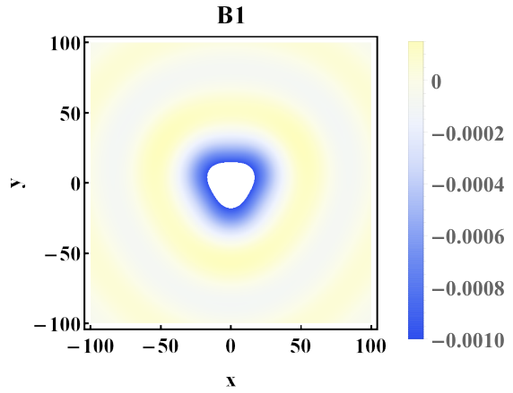
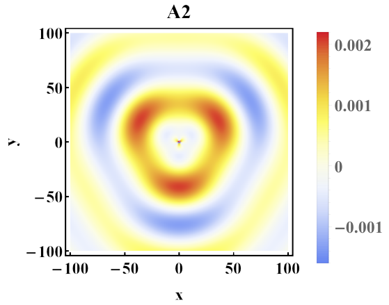
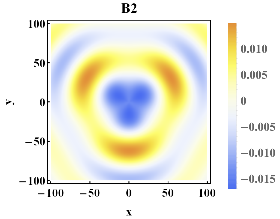
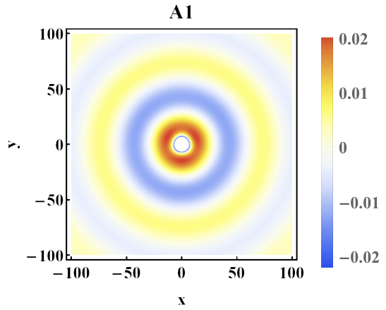
Considering the form of the $T$ -matrix presented in Eq. (12), we can calculate analytically via Eq. (17) the corrections to the local density of states induced by each type of impuritiy. The exact analytical expressions for $\delta\rho_{A1}(\epsilon,r,\phi_{r})$ , $\delta\rho_{B1}(\epsilon,r,\phi_{r})$ , $\delta\rho_{A2}(\epsilon,r,\phi_{r})$ , and $\delta\rho_{B2}(\epsilon,r,\phi_{r})$ can be found using Eq. 17 and the Appendixes. We plot the corresponding expressions in Fig. 2.

We can clearly see that the figures for A2 and B2 impurities show strong threefold-symmetric features originating from the trigonal warping terms. Using the asymptotic forms of the local density of states calculated at $r\to+\infty$ from Eqs. (71-74), we present below their simplified forms at energies such that $0<\epsilon\ll\gamma_{01}$ . In this range of energies we can neglect the exponentially fast decaying terms, i.e., the terms containing $e^{-2\Omega_{+}r}$ factors, and thus we get:

\displaystyle\delta\rho_{A1}=\frac{1}{\pi}\im\left[\frac{f(\epsilon)}{32\pi\epsilon}\Omega_{-}\frac{\gamma_{01}+\gamma_{03}\Omega_{-}\sin 3\phi_{r}}{r}e^{-2\Omega_{-}r}\right]

(18)

\displaystyle\delta\rho_{B1}=\frac{1}{\pi}\im\left[\frac{g(\epsilon)}{32\pi}\gamma_{01}\frac{\epsilon+\gamma_{03}\Omega_{-}\sin 3\phi_{r}}{\Omega_{-}r}e^{-2\Omega_{-}r}\right]

(19)

\displaystyle\delta\rho_{A2}=\frac{1}{\pi}\im\left[\frac{g(\epsilon)}{32\pi}\gamma_{01}\frac{\epsilon-\gamma_{03}\Omega_{-}\sin 3\phi_{r}}{\Omega_{-}r}e^{-2\Omega_{-}r}\right]

(20)

\displaystyle\delta\rho_{B2}=-\frac{1}{\pi}\im\left[\frac{f(\epsilon)}{32\pi}\gamma_{01}\frac{\gamma_{01}-\gamma_{03}\Omega_{-}\sin 3\phi_{r}}{\Omega_{-}r}e^{-2\Omega_{-}r}\right]

(21)

Note, that for negative energies $\epsilon<0$ we should keep the terms with $e^{-2\Omega_{+}r}$ factors and discard those with $e^{-2\Omega_{-}r}$ . Furthermore, it is worth emphasizing that the asymptotic expansions above describe the LDOS well only at large distances from the origin, namely, at $r\gg\mathrm{max}(\frac{1}{2|\Omega_{+}|},\frac{1}{2|\Omega_{-}|})$ . Therefore, to recover correctly the features in the vicinity of the impurity we have to consider the full expressions provided in Eqs. (71-74).

The results presented in Fig. 2 are in a nearly perfect agreement with the semi-analytical $T$ -matrix calculations based on a lattice model and presented in Ref. [Joucken et al. 2021].

Furthermore, the orientation of the triangles flips with the sign of $\gamma_{03}$ . This can be straightforwardly seen in the asymptotic forms of the corrections derived in Eqs. (18-21) for $r\to+\infty$ , that can be rewritten in a simplified form

\displaystyle\delta\rho\sim\frac{\alpha+\beta\gamma_{03}\sin 3\phi_{r}}{r}e^{-\Omega r},

(22)

where $\alpha,\beta$ and $\Omega$ can be inferred from Eqs. (18-21).

In the equation above the term generated by trigonal warping is proportional to $\sin 3\phi_{r}/r$ , while the first term proportional to $1/r$ is known in the literature as the quasiparticle interference pattern for bilayer graphene in the absence of trigonal warping Bena 2008.

We should note, as expected from the band structure, the smaller the energy at which we calculate the quasiparticle interference patterns, the more visible are the effects of the trigonal warping.

IV.2.2 Momentum space

In what follows we analyze theoretically momentum-space quasiparticle interference patterns experimentally accessible via Fourier-transform scanning tunneling microscopy. It is clear that the Fourier transform of Eq. (22) yields both rotationally symmetric and angular-dependent parts. We Fourier-transform Eqs. (18-21) and we get:

$\displaystyle\delta\rho_{A1}$	$\displaystyle=\frac{1}{2\pi i}\frac{f(\epsilon)\Omega_{-}\left[\gamma_{01}\mathcal{F}_{0}(p,2\Omega_{-})+\gamma_{03}\Omega_{-}\mathcal{F}_{1}(\bm{p},2\Omega_{-})\right]-f^{}(\epsilon)\Omega^{}_{-}\left[\gamma_{01}\mathcal{F}_{0}(p,2\Omega^{}_{-})+\gamma_{03}\Omega^{}_{-}\mathcal{F}_{1}(\bm{p},2\Omega^{*}_{-})\right]}{32\pi\epsilon},$	(23)
$\displaystyle\delta\rho_{B1}$	$\displaystyle=\frac{1}{2\pi i}\gamma_{01}\frac{\frac{g(\epsilon)}{\Omega_{-}}\left[\epsilon\mathcal{F}_{0}(p,2\Omega_{-})+\gamma_{03}\Omega_{-}\mathcal{F}_{1}(\bm{p},2\Omega_{-})\right]-\frac{g^{}(\epsilon)}{\Omega^{}_{-}}\left[\epsilon\mathcal{F}_{0}(p,2\Omega^{}_{-})+\gamma_{03}\Omega^{}_{-}\mathcal{F}_{1}(\bm{p},2\Omega^{*}_{-})\right]}{32\pi},$	(24)
$\displaystyle\delta\rho_{A2}$	$\displaystyle=\frac{1}{2\pi i}\gamma_{01}\frac{\frac{g(\epsilon)}{\Omega_{-}}\left[\epsilon\mathcal{F}_{0}(p,2\Omega_{-})-\gamma_{03}\Omega_{-}\mathcal{F}_{1}(\bm{p},2\Omega_{-})\right]-\frac{g^{}(\epsilon)}{\Omega^{}_{-}}\left[\epsilon\mathcal{F}_{0}(p,2\Omega^{}_{-})-\gamma_{03}\Omega^{}_{-}\mathcal{F}_{1}(\bm{p},2\Omega^{*}_{-})\right]}{32\pi},$	(25)
$\displaystyle\delta\rho_{B2}$	$\displaystyle=-\frac{1}{2\pi i}\gamma_{01}\frac{\frac{f(\epsilon)}{\Omega_{-}}\left[\gamma_{01}\mathcal{F}_{0}(p,2\Omega_{-})-\gamma_{03}\Omega_{-}\mathcal{F}_{1}(\bm{p},2\Omega_{-})\right]-\frac{f^{}(\epsilon)}{\Omega^{}_{-}}\left[\gamma_{01}\mathcal{F}_{0}(p,2\Omega^{}_{-})-\gamma_{03}\Omega^{}_{-}\mathcal{F}_{1}(\bm{p},2\Omega^{*}_{-})\right]}{32\pi},$	(26)

where $\mathcal{F}_{0}$ and $\mathcal{F}_{1}$ are calculated in Appendix D, and are given by:

		$\displaystyle\mathcal{F}_{0}(p,\Omega)=\frac{2\pi}{\Omega}\frac{1}{\sqrt{1+\frac{p^{2}}{\Omega^{2}}}}$		(27)
		$\displaystyle\mathcal{F}_{1}(\bm{p},\Omega)=2\pi i\sin 3\phi_{p}\times$
		$\displaystyle\frac{p^{2}\left(-3+\sqrt{1+\frac{p^{2}}{\Omega^{2}}}\right)+4\Omega^{2}\left(-1+\sqrt{1+\frac{p^{2}}{\Omega^{2}}}\right)}{p^{3}\sqrt{1+\frac{p^{2}}{\Omega^{2}}}}$		(28)

Using these definitions and the Fourier transforms in Eqs. (23-26) we infer the position of the ring-like resonance in momentum space

\displaystyle p_{\mathrm{res}}=-2i\Omega_{-}=2\sqrt{\epsilon(\gamma_{01}+\epsilon)}.

(29)

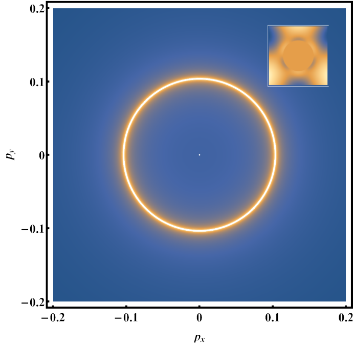
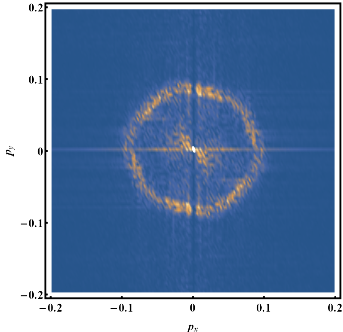
Above we denoted $\epsilon\equiv\frac{2E}{\gamma_{0}\sqrt{3}}$ , where $E$ is the energy at which we calculate the response. On the left panel in Fig. 3 we plot the absolute of the sum of Fourier transforms in Eqs. (23-26) simulating a large-sample experiment in which all types of impurities contribute to the local response. On the right panel of Fig. 3 we show the corresponding experimental measurement in dimensionless momentum space $(p_{x},p_{y})=(k_{x}a,k_{y}a)$ , where the lattice constant $a=2.46\,$ Å. We see that the analytical and experimental results are in a good agreement, i.e., $p^{\mathrm{exp}}_{\mathrm{res}}\approx 0.095$ is very close to the analytically calculated value using Eq. (29):

\displaystyle p_{\mathrm{res}}=2\sqrt{\frac{2E}{\gamma_{0}\sqrt{3}}\left(\frac{2\gamma_{1}}{\gamma_{0}\sqrt{3}}+\frac{2E}{\gamma_{0}\sqrt{3}}\right)}\approx 0.1,

(30)

where we set $E=47\,$ meV.

To derive the FT LDOS we used the asymptotic expansions in Eqs. (18-21), and since we work with asymptotic expansions at $r\to+\infty$ obtained within a low-energy approximation, the hexagonal shape of the resonance is lost in the analytically computed FT versus the experimental one (left versus right panels of Fig. 3). In Eqs. (23-26) the reminiscence of hexagonal symmetries is carried solely by the phase factor $\sin 3\phi_{p}$ in the definition of $\mathcal{F}_{1}(\bm{p},\Omega)$ , and it is reflected in the inset of the left panel.

The results obtained above are also qualitatively consistent with the numerical $T$ -matrix calculations presented in Ref. [Joucken et al. 2021], with the only difference being the hexagonal shape of the resonance in the latter. This discrepancy stems from the fact that in this work we use a low-energy approximation, while the numerical $T$ -matrix calculations were performed within a lattice model.

V Conclusions

We have calculated analytically the form of the quasiparticle interference patterns in bilayer graphene for four types of impurities localized on different layers and sublattices, taking into account perturbatively the trigonal warping of the bands. First and foremost, our results both in real space and in Fourier space are in good agreement with the experimental measurements and $T$ -matrix-based semi-analytical simulations of such patterns Joucken et al. 2020; Joucken et al. 2021. Most importantly the fact that our analytical results can be expressed in closed form provides us with an understanding of the origin of the observed triangular features in real space. Thus, we clearly see that they originate in the trigonal warping terms and flip orientation when the trigonal warping is changing sign. Also our results allow us to predict the value of the momentum corresponding to the ring-like resonances visible in momentum space and to the real-space oscillations; this seems to be independent of the value of the trigonal warping.

Acknowledgements.

J.V.J. acknowledges support from the National Science Foundation under award DMR-1753367 and the Army Research Office under contract W911NF-17-1-0473.

References

Friedel (1958) J. Friedel, Il Nuovo Cimento 7, 10.1007/bf02751483 (1958).
Cheianov and Fal’ko (2006) V. V. Cheianov and V. I. Fal’ko, Phys. Rev. Lett. 97, 226801 (2006).
Mariani et al. (2007) E. Mariani, L. I. Glazman, A. Kamenev, and F. von Oppen, Phys. Rev. B 76, 165402 (2007).
Kivelson et al. (2003) S. A. Kivelson, I. P. Bindloss, E. Fradkin, V. Oganesyan, J. M. Tranquada, A. Kapitulnik, and C. Howald, Rev. Mod. Phys. 75, 1201 (2003).
Bena and Kivelson (2005) C. Bena and S. A. Kivelson, Phys. Rev. B 72, 125432 (2005).
Bena (2008) C. Bena, Phys. Rev. Lett. 100, 076601 (2008).
Bena (2009) C. Bena, Phys. Rev. B 79, 125427 (2009).
Wehling et al. (2007) T. O. Wehling, A. V. Balatsky, M. I. Katsnelson, A. I. Lichtenstein, K. Scharnberg, and R. Wiesendanger, Phys. Rev. B 75, 125425 (2007).
Peres et al. (2006) N. M. R. Peres, F. Guinea, and A. H. Castro Neto, Phys. Rev. B 73, 125411 (2006).
Peres et al. (2007) N. M. R. Peres, F. D. Klironomos, S.-W. Tsai, J. R. Santos, J. M. B. L. dos Santos, and A. H. C. Neto, Europhysics Letters (EPL) 80, 67007 (2007).
Vozmediano et al. (2005) M. A. H. Vozmediano, M. P. López-Sancho, T. Stauber, and F. Guinea, Phys. Rev. B 72, 155121 (2005).
Ando (2006) T. Ando, Journal of the Physical Society of Japan 75, 074716 (2006).
Pogorelov (2006) Y. Pogorelov, arXiv:0603327 (2006).
Skrypnyk and Loktev (2006) Y. V. Skrypnyk and V. M. Loktev, Phys. Rev. B 73, 241402 (2006).
Skrypnyk and Loktev (2007) Y. V. Skrypnyk and V. M. Loktev, Phys. Rev. B 75, 245401 (2007).
Katsnelson and Geim (2007) M. Katsnelson and A. Geim, Philosophical Transactions of the Royal Society A: Mathematical, Physical and Engineering Sciences 366, 195 (2007).
Dutreix and Katsnelson (2016) C. Dutreix and M. I. Katsnelson, Phys. Rev. B 93, 035413 (2016).
Mallet et al. (2007) P. Mallet, F. Varchon, C. Naud, L. Magaud, C. Berger, and J.-Y. Veuillen, Phys. Rev. B 76, 041403 (2007).
Mallet et al. (2016) P. Mallet, I. Brihuega, V. Cherkez, J. M. Gómez-Rodríguez, and J.-Y. Veuillen, Comptes Rendus Physique 17, 294 (2016).
Charlier et al. (1991) J.-C. Charlier, X. Gonze, and J.-P. Michenaud, Phys. Rev. B 43, 4579 (1991).
McCann and Fal’ko (2006) E. McCann and V. I. Fal’ko, Phys. Rev. Lett. 96, 086805 (2006).
McCann and Koshino (2013) E. McCann and M. Koshino, Reports on Progress in Physics 76, 056503 (2013).
Kuzmenko et al. (2009) A. B. Kuzmenko, I. Crassee, D. van der Marel, P. Blake, and K. S. Novoselov, Phys. Rev. B 80, 165406 (2009).
Joucken et al. (2020) F. Joucken, Z. Ge, E. A. Quezada-López, J. L. Davenport, K. Watanabe, T. Taniguchi, and J. Velasco, Phys. Rev. B 101, 161103 (2020).
Zibrov et al. (2018) A. A. Zibrov, P. Rao, C. Kometter, E. M. Spanton, J. I. A. Li, C. R. Dean, T. Taniguchi, K. Watanabe, M. Serbyn, and A. F. Young, Phys. Rev. Lett. 121, 167601 (2018).
Varlet et al. (2014) A. Varlet, D. Bischoff, P. Simonet, K. Watanabe, T. Taniguchi, T. Ihn, K. Ensslin, M. Mucha-Kruczyński, and V. I. Fal’ko, Phys. Rev. Lett. 113, 116602 (2014).
Orlita et al. (2012) M. Orlita, P. Neugebauer, C. Faugeras, A.-L. Barra, M. Potemski, F. M. D. Pellegrino, and D. M. Basko, Phys. Rev. Lett. 108, 017602 (2012).
Shi et al. (2018) Y. Shi, S. Che, K. Zhou, S. Ge, Z. Pi, T. Espiritu, T. Taniguchi, K. Watanabe, Y. Barlas, R. Lake, and C. N. Lau, Phys. Rev. Lett. 120, 096802 (2018).
Kechedzhi et al. (2007) K. Kechedzhi, V. I. Fal’ko, E. McCann, and B. L. Altshuler, Phys. Rev. Lett. 98, 176806 (2007).
Ge et al. (2020) Z. Ge, F. Joucken, E. Quezada, D. R. da Costa, J. Davenport, B. Giraldo, T. Taniguchi, K. Watanabe, N. P. Kobayashi, T. Low, and J. Velasco, Nano Letters 20, 8682 (2020).
Jung and MacDonald (2014) J. Jung and A. H. MacDonald, Phys. Rev. B 89, 035405 (2014).
Byers et al. (1993) J. M. Byers, M. E. Flatté, and D. J. Scalapino, Phys. Rev. Lett. 71, 3363 (1993).
Salkola et al. (1996) M. I. Salkola, A. V. Balatsky, and D. J. Scalapino, Phys. Rev. Lett. 77, 1841 (1996).
Ziegler et al. (1996) W. Ziegler, D. Poilblanc, R. Preuss, W. Hanke, and D. J. Scalapino, Phys. Rev. B 53, 8704 (1996).
Mahan (2000) G. D. Mahan, Many-Particle Physics (Springer US, 2000).
Balatsky et al. (2006) A. V. Balatsky, I. Vekhter, and J.-X. Zhu, Rev. Mod. Phys. 78, 373 (2006).
Bena (2016) C. Bena, Comptes Rendus Physique 17, 302 (2016).
Joucken et al. (2021) F. Joucken, C. Bena, Z. Ge, E. A. Quezada-López, S. Pinon, V. Kaladzhyan, K. Taniguchi, T. Watanabe, and J. Velasco Jr, arXiv:2104.10620 (2021).

Appendix A Green’s functions in momentum space

A.1 0-th order

\displaystyle G_{0}(i\omega,\bm{q})=\frac{1}{(q^{2}-(i\omega)^{2}+i\omega\gamma_{01})(q^{2}-(i\omega)^{2}-i\omega\gamma_{01})}\begin{pmatrix}g_{0}^{11}&\left(g_{0}^{21}\right)^{\star}&\left(g_{0}^{31}\right)^{\star}&\left(g_{0}^{41}\right)^{\star}\\ g_{0}^{21}&g_{0}^{22}&g_{0}^{32}&\left(g_{0}^{31}\right)^{\star}\\ g_{0}^{31}&g_{0}^{32}&g_{0}^{22}&\left(g_{0}^{21}\right)^{\star}\\ g_{0}^{41}&g_{0}^{31}&g_{0}^{21}&g_{0}^{11}\end{pmatrix},

(31)

with $g_{0}^{ij}$ denoting the $(ij)$ -th element of the matrix $g_{0}$ .

		$\displaystyle g_{0}^{11}\equiv i\omega((i\omega)^{2}-\gamma_{01}^{2})-i\omega q^{2},\;g_{0}^{22}\equiv(i\omega)^{3}-(i\omega)q^{2},\;g_{0}^{21}\equiv(i\omega)^{2}\cdot sqe^{is\phi_{q}}-sq^{3}e^{is\phi_{q}},\;g_{0}^{31}\equiv i\omega\gamma_{01}\cdot sqe^{is\phi_{q}},$
		$\displaystyle g_{0}^{32}\equiv(i\omega)^{2}\gamma_{01},\;g_{0}^{41}\equiv\gamma_{01}\cdot q^{2}e^{2is\phi_{q}}.$		(32)

The symbol $\star$ denotes replacing $\phi_{q}\to-\phi_{q}$ , e.g., $\left(g_{0}^{31}\right)^{\star}=i\omega\gamma_{01}\cdot sqe^{-is\phi_{q}}$ .

A.2 1-st order

The first-order correction in trigonal warping is given by

\displaystyle G_{1}(i\omega,\bm{q})=\frac{\gamma_{03}}{(q^{2}-(i\omega)^{2}+i\omega\gamma_{01})^{2}(q^{2}-(i\omega)^{2}-i\omega\gamma_{01})^{2}}\begin{pmatrix}g_{1}^{11}&\left(g_{1}^{21}\right)^{\star}&\left(g_{1}^{31}\right)^{\star}&\left(g_{1}^{41}\right)^{\star}\\ g_{1}^{21}&g_{1}^{22}&\left(g_{1}^{32}\right)^{\star}&\left(g_{1}^{31}\right)^{\star}\\ g_{1}^{31}&g_{1}^{32}&g_{1}^{22}&\left(g_{1}^{21}\right)^{\star}\\ g_{1}^{41}&g_{1}^{31}&g_{1}^{21}&g_{1}^{11}\end{pmatrix},

where

$\displaystyle g_{1}^{11}$	$\displaystyle\equiv-\gamma_{01}i\omega\left[sq^{5}e^{3is\phi_{q}}+sq^{5}e^{-3is\phi_{q}}\right]-\gamma_{01}i\omega(\gamma_{01}^{2}-(i\omega)^{2})\left[sq^{3}e^{3is\phi_{q}}+sq^{3}e^{-3is\phi_{q}}\right]$	(33)
$\displaystyle g_{1}^{22}$	$\displaystyle\equiv-\gamma_{01}i\omega\left[sq^{5}e^{3is\phi_{q}}+sq^{5}e^{-3is\phi_{q}}\right]+\gamma_{01}(i\omega)^{3}\left[sq^{3}e^{3is\phi_{q}}+sq^{3}e^{-3is\phi_{q}}\right],$	(34)
$\displaystyle g_{1}^{21}$	$\displaystyle\equiv-\gamma_{01}\left[q^{6}e^{4is\phi_{q}}\right]+\gamma_{01}(i\omega)^{2}\left[q^{4}e^{4is\phi_{q}}-q^{4}e^{-2is\phi_{q}}\right]-\gamma_{01}(i\omega)^{2}(\gamma_{01}^{2}-(i\omega)^{2})\left[q^{2}e^{-2is\phi_{q}}\right],$	(35)
$\displaystyle g_{1}^{31}$	$\displaystyle\equiv i\omega\left[q^{6}e^{-2is\phi_{q}}\right]+\gamma_{01}^{2}i\omega\left[q^{4}e^{4is\phi_{q}}\right]+i\omega(\gamma_{01}^{2}-2(i\omega)^{2})\left[q^{4}e^{-2is\phi_{q}}\right]-(i\omega)^{3}(\gamma_{01}^{2}-(i\omega)^{2})\left[q^{2}e^{-2is\phi_{q}}\right],$	(36)
$\displaystyle g_{1}^{32}$	$\displaystyle\equiv\left[sq^{7}e^{-3is\phi_{q}}\right]-2(i\omega)^{2}\left[sq^{5}e^{-3is\phi_{q}}\right]+(i\omega)^{4}\left[sq^{3}e^{-3is\phi_{q}}\right]+\gamma_{01}^{2}(i\omega)^{2}\left[sq^{3}e^{3is\phi_{q}}\right],$	(37)
$\displaystyle g_{1}^{41}$	$\displaystyle\equiv\gamma_{01}^{2}\left[sq^{5}e^{5is\phi_{q}}\right]+(i\omega)^{2}\left[sq^{5}e^{-is\phi_{q}}\right]+2(i\omega)^{2}(\gamma_{01}^{2}-(i\omega)^{2})\left[sq^{3}e^{-is\phi_{q}}\right]+(i\omega)^{2}(\gamma_{01}^{2}-(i\omega)^{2})^{2}\left[sqe^{-is\phi_{q}}\right].$	(38)

Appendix B Integrals to define Green’s functions in real space

B.1 Integrals for the 0-th order

We can write the 0-th order Green’s function in real space as follows:

\displaystyle G_{0}(i\omega,\bm{r})=\begin{pmatrix}i\omega((i\omega)^{2}-\gamma_{01}^{2})I_{00}-i\omega I_{03}&(i\omega)^{2}I^{-}_{01}-I_{04}^{-}&\gamma_{01}i\omega I_{01}^{-}&\gamma_{01}I_{02}^{-}\\ (i\omega)^{2}I^{+}_{01}-I_{04}^{+}&i\omega^{3}I_{00}-i\omega I_{03}&\gamma_{01}(i\omega)^{2}I_{00}&\gamma_{01}i\omega I_{01}^{-}\\ \gamma_{01}i\omega I_{01}^{+}&\gamma_{01}(i\omega)^{2}I_{00}&i\omega^{3}I_{00}-i\omega I_{03}&(i\omega)^{2}I^{-}_{01}-I_{04}^{-}\\ \gamma_{01}I_{02}^{+}&\gamma_{01}i\omega I_{01}^{+}&(i\omega)^{2}I^{+}_{01}-I_{04}^{+}&i\omega((i\omega)^{2}-\gamma_{01}^{2})I_{00}-i\omega I_{03}\end{pmatrix}

(39)

$\displaystyle I_{00}$	$\displaystyle=\int\limits_{0}^{+\infty}\frac{qdq}{2\pi}\int\limits_{0}^{2\pi}\frac{d\phi_{q}}{2\pi}\frac{e^{iqr\cos(\phi_{q}-\phi_{r})}}{(q^{2}-(i\omega)^{2}+\gamma_{01}i\omega)(q^{2}-(i\omega)^{2}-\gamma_{01}i\omega)}=\int\limits_{0}^{+\infty}\frac{dq}{2\pi}\frac{qJ_{0}(qr)}{(q^{2}-(i\omega)^{2}+\gamma_{01}i\omega)(q^{2}-(i\omega)^{2}-\gamma_{01}i\omega)}=$
	$\displaystyle=-\frac{1}{4\pi\gamma_{01}i\omega}\left[K_{0}(\Omega_{+}r)-K_{0}(\Omega_{-}r)\right]$	(40)
$\displaystyle I^{\pm}_{01}$	$\displaystyle=\int\limits_{0}^{+\infty}\frac{qdq}{2\pi}\int\limits_{0}^{2\pi}\frac{d\phi_{q}}{2\pi}\frac{sqe^{\pm is\phi_{q}}e^{iqr\cos(\phi_{q}-\phi_{r})}}{(q^{2}-(i\omega)^{2}+\gamma_{01}i\omega)(q^{2}-(i\omega)^{2}-\gamma_{01}i\omega)}=\int\limits_{0}^{+\infty}\frac{dq}{2\pi}\frac{ise^{\pm is\phi_{r}}q^{2}J_{1}(qr)}{(q^{2}-(i\omega)^{2}+\gamma_{01}i\omega)(q^{2}-(i\omega)^{2}-\gamma_{01}i\omega)}=$
	$\displaystyle=-\frac{ise^{\pm is\phi_{r}}}{4\pi\gamma_{01}i\omega_{n}}\left[\Omega_{+}K_{1}(\Omega_{+}r)-\Omega_{-}K_{1}(\Omega_{-}r)\right]$	(41)
$\displaystyle I^{\pm}_{02}$	$\displaystyle=\int\limits_{0}^{+\infty}\frac{qdq}{2\pi}\int\limits_{0}^{2\pi}\frac{d\phi_{q}}{2\pi}\frac{q^{2}e^{\pm 2is\phi_{q}}e^{iqr\cos(\phi_{q}-\phi_{r})}}{(q^{2}-(i\omega)^{2}+\gamma_{01}i\omega)(q^{2}-(i\omega)^{2}-\gamma_{01}i\omega)}=\int\limits_{0}^{+\infty}\frac{dq}{2\pi}\frac{-e^{\pm 2is\phi_{r}}q^{3}J_{2}(qr)}{(q^{2}-(i\omega)^{2}+\gamma_{01}i\omega)(q^{2}-(i\omega)^{2}-\gamma_{01}i\omega)}=$
	$\displaystyle=\frac{e^{\pm 2is\phi_{r}}}{4\pi\gamma_{01}i\omega}\left[\Omega_{+}^{2}K_{2}(\Omega_{+}r)-\Omega_{-}^{2}K_{2}(\Omega_{-}r)\right]$	(42)
$\displaystyle I_{03}$	$\displaystyle=\int\limits_{0}^{+\infty}\frac{qdq}{2\pi}\int\limits_{0}^{2\pi}\frac{d\phi_{q}}{2\pi}\frac{q^{2}e^{iqr\cos(\phi_{q}-\phi_{r})}}{(q^{2}-(i\omega)^{2}+\gamma_{01}i\omega)(q^{2}-(i\omega)^{2}-\gamma_{01}i\omega)}=\int\limits_{0}^{+\infty}\frac{dq}{2\pi}\frac{q^{3}J_{0}(qr)}{(q^{2}-(i\omega)^{2}+\gamma_{01}i\omega)(q^{2}-(i\omega)^{2}-\gamma_{01}i\omega)}=$
	$\displaystyle=\frac{1}{4\pi\gamma_{01}i\omega}\left[\Omega_{+}^{2}K_{0}(\Omega_{+}r)-\Omega_{-}^{2}K_{0}(\Omega_{-}r)\right]$	(43)
$\displaystyle I^{\pm}_{04}$	$\displaystyle=\int\limits_{0}^{+\infty}\frac{qdq}{2\pi}\int\limits_{0}^{2\pi}\frac{d\phi_{q}}{2\pi}\frac{sq^{3}e^{\pm is\phi_{q}}e^{iqr\cos(\phi_{q}-\phi_{r})}}{(q^{2}-(i\omega)^{2}+\gamma_{01}i\omega)(q^{2}-(i\omega)^{2}-\gamma_{01}i\omega)}=\int\limits_{0}^{+\infty}\frac{dq}{2\pi}\frac{ise^{\pm is\phi_{r}}q^{4}J_{1}(qr)}{(q^{2}-(i\omega)^{2}+\gamma_{01}i\omega)(q^{2}-(i\omega)^{2}-\gamma_{01}i\omega)}=$
	$\displaystyle=\frac{ise^{\pm is\phi_{r}}}{4\pi\gamma_{01}i\omega}\left[\Omega_{+}^{3}K_{1}(\Omega_{+}r)-\Omega_{-}^{3}K_{1}(\Omega_{-}r)\right],$	(44)

where we denoted $\Omega_{\pm}=\sqrt{i\omega(\pm\gamma_{01}-i\omega)},$ and $K_{i}(z)$ is the $i$ -th modified Bessel function of the second kind.

B.2 Integrals for the 1-st order

We can write component-wise the 1-st order Green’s function in real space as follows:

$\displaystyle G^{11}_{1}$	$\displaystyle=\gamma_{03}\left[-\gamma_{01}i\omega(I_{53}^{+}+I_{53}^{-})-\gamma_{01}i\omega(\gamma_{01}^{2}-(i\omega)^{2})(I_{33}^{+}+I_{33}^{-})\right],$	(45)
$\displaystyle G^{22}_{1}$	$\displaystyle=\gamma_{03}\left[-\gamma_{01}i\omega(I_{53}^{+}+I_{53}^{-})+\gamma_{01}(i\omega)^{3}(I_{33}^{+}+I_{33}^{-})\right],$	(46)
$\displaystyle G^{21}_{1}$	$\displaystyle=\gamma_{03}\left[-\gamma_{01}I_{64}^{+}+\gamma_{01}(i\omega)^{2}(I_{44}^{+}-I_{42}^{-})-\gamma_{01}(i\omega)^{2}(\gamma_{01}^{2}-(i\omega)^{2})I_{22}^{-}\right],$	(47)
$\displaystyle G^{31}_{1}$	$\displaystyle=\gamma_{03}\left[i\omega I_{62}^{-}+\gamma_{01}^{2}i\omega I_{44}^{+}+i\omega(\gamma_{01}^{2}-2(i\omega)^{2})I_{42}^{-}-(i\omega)^{3}(\gamma_{01}^{2}-(i\omega)^{2})I_{22}^{-}\right],$	(48)
$\displaystyle G^{32}_{1}$	$\displaystyle=\gamma_{03}\left[I_{73}^{-}-2(i\omega)^{2}I_{53}^{-}+(i\omega)^{4}I_{33}^{-}+\gamma_{01}^{2}(i\omega)^{2}I_{33}^{+}\right],$	(49)
$\displaystyle G^{41}_{1}$	$\displaystyle=\gamma_{03}\left[\gamma_{01}^{2}I_{55}^{+}+(i\omega)^{2}I_{51}^{-}+2(i\omega)^{2}(\gamma_{01}^{2}-(i\omega)^{2})I_{31}^{-}+(i\omega)^{2}(\gamma_{01}^{2}-(i\omega)^{2})^{2}I_{11}^{-}\right],$	(50)
$\displaystyle G^{33}_{1}$	$\displaystyle=G^{22}_{1},\,G^{44}_{1}=G^{11}_{1},\,G^{42}_{1}=G^{31}_{1},\,G^{43}_{1}=G^{21}_{1},$	(51)
$\displaystyle G^{12}_{1}$	$\displaystyle=G^{34}_{1}=G^{21}_{1}(+\leftrightarrow-),\,G^{13}_{1}=G^{24}_{1}=G^{31}_{1}(+\leftrightarrow-),\,G^{14}_{1}=G^{41}_{1}(+\leftrightarrow-),\,G^{23}_{1}=G^{32}_{1}(+\leftrightarrow-).$	(52)

$\displaystyle I^{\pm}_{11}$	$\displaystyle=\int\limits_{0}^{+\infty}\frac{qdq}{2\pi}\int\limits_{0}^{2\pi}\frac{d\phi_{q}}{2\pi}\frac{sqe^{\pm is\phi_{q}}e^{iqr\cos(\phi_{q}-\phi_{r})}}{(q^{2}-(i\omega)^{2}+\gamma_{01}i\omega)^{2}(q^{2}-(i\omega)^{2}-\gamma_{01}i\omega)^{2}}=\int\limits_{0}^{+\infty}\frac{dq}{2\pi}\frac{ise^{\pm is\phi_{r}}q^{2}J_{1}(qr)}{(q^{2}-(i\omega)^{2}+\gamma_{01}i\omega)^{2}(q^{2}-(i\omega)^{2}-\gamma_{01}i\omega)^{2}}=$
	$\displaystyle=\frac{ise^{\pm is\phi_{r}}}{16\pi\gamma_{01}^{3}(i\omega)^{3}}\left[2\left(\Omega_{+}K_{1}(\Omega_{+}r)-\Omega_{-}K_{1}(\Omega_{-}r)\right)+i\omega\gamma_{01}r\left(K_{0}(\Omega_{+}r)+K_{0}(\Omega_{-}r)\right)\right]$	(53)
$\displaystyle I^{\pm}_{31}$	$\displaystyle=\int\limits_{0}^{+\infty}\frac{qdq}{2\pi}\int\limits_{0}^{2\pi}\frac{d\phi_{q}}{2\pi}\frac{sq^{3}e^{\pm is\phi_{q}}e^{iqr\cos(\phi_{q}-\phi_{r})}}{(q^{2}-(i\omega)^{2}+\gamma_{01}i\omega)^{2}(q^{2}-(i\omega)^{2}-\gamma_{01}i\omega)^{2}}=\int\limits_{0}^{+\infty}\frac{dq}{2\pi}\frac{ise^{\pm is\phi_{r}}q^{4}J_{1}(qr)}{(q^{2}-(i\omega)^{2}+\gamma_{01}i\omega)^{2}(q^{2}-(i\omega)^{2}-\gamma_{01}i\omega)^{2}}=$
	$\displaystyle=\frac{ise^{\pm is\phi_{r}}}{16\pi\gamma_{01}^{3}(i\omega)^{2}}\left[2i\omega\left(\Omega_{+}K_{1}(\Omega_{+}r)-\Omega_{-}K_{1}(\Omega_{-}r)\right)-\gamma_{01}r\left(\Omega_{+}^{2}K_{0}(\Omega_{+}r)+\Omega_{-}^{2}K_{0}(\Omega_{-}r)\right)\right]$	(54)
$\displaystyle I^{\pm}_{51}$	$\displaystyle=\int\limits_{0}^{+\infty}\frac{qdq}{2\pi}\int\limits_{0}^{2\pi}\frac{d\phi_{q}}{2\pi}\frac{sq^{5}e^{\pm is\phi_{q}}e^{iqr\cos(\phi_{q}-\phi_{r})}}{(q^{2}-(i\omega)^{2}+\gamma_{01}i\omega)^{2}(q^{2}-(i\omega)^{2}-\gamma_{01}i\omega)^{2}}=\int\limits_{0}^{+\infty}\frac{dq}{2\pi}\frac{ise^{\pm is\phi_{r}}q^{6}J_{1}(qr)}{(q^{2}-(i\omega)^{2}+\gamma_{01}i\omega)^{2}(q^{2}-(i\omega)^{2}-\gamma_{01}i\omega)^{2}}=$
	$\displaystyle=\frac{ise^{\pm is\phi_{r}}}{16\pi\gamma_{01}^{3}(i\omega)^{2}}\left[2i\omega(\gamma_{01}^{2}-(i\omega)^{2})\left(\Omega_{-}K_{1}(\Omega_{-}r)-\Omega_{+}K_{1}(\Omega_{+}r)\right)+\gamma_{01}r\left(\Omega_{+}^{4}K_{0}(\Omega_{+}r)+\Omega_{-}^{4}K_{0}(\Omega_{-}r)\right)\right]$	(55)
$\displaystyle I^{\pm}_{22}$	$\displaystyle=\int\limits_{0}^{+\infty}\frac{qdq}{2\pi}\int\limits_{0}^{2\pi}\frac{d\phi_{q}}{2\pi}\frac{q^{2}e^{\pm 2is\phi_{q}}e^{iqr\cos(\phi_{q}-\phi_{r})}}{(q^{2}-(i\omega)^{2}+\gamma_{01}i\omega)^{2}(q^{2}-(i\omega)^{2}-\gamma_{01}i\omega)^{2}}=\int\limits_{0}^{+\infty}\frac{dq}{2\pi}\frac{-e^{\pm 2is\phi_{r}}q^{3}J_{2}(qr)}{(q^{2}-(i\omega)^{2}+\gamma_{01}i\omega)^{2}(q^{2}-(i\omega)^{2}-\gamma_{01}i\omega)^{2}}=$
	$\displaystyle=-\frac{e^{\pm 2is\phi_{r}}}{16\pi\gamma_{01}^{3}(i\omega)^{3}}\left[2\left(\Omega_{+}^{2}K_{2}(\Omega_{+}r)-\Omega_{-}^{2}K_{2}(\Omega_{-}r)\right)+i\omega\gamma_{01}r\left(\Omega_{+}K_{1}(\Omega_{+}r)+\Omega_{-}K_{1}(\Omega_{-}r)\right)\right]$	(56)
$\displaystyle I^{\pm}_{42}$	$\displaystyle=\int\limits_{0}^{+\infty}\frac{qdq}{2\pi}\int\limits_{0}^{2\pi}\frac{d\phi_{q}}{2\pi}\frac{q^{4}e^{\pm 2is\phi_{q}}e^{iqr\cos(\phi_{q}-\phi_{r})}}{(q^{2}-(i\omega)^{2}+\gamma_{01}i\omega)^{2}(q^{2}-(i\omega)^{2}-\gamma_{01}i\omega)^{2}}=\int\limits_{0}^{+\infty}\frac{dq}{2\pi}\frac{-e^{\pm 2is\phi_{r}}q^{5}J_{2}(qr)}{(q^{2}-(i\omega)^{2}+\gamma_{01}i\omega)^{2}(q^{2}-(i\omega)^{2}-\gamma_{01}i\omega)^{2}}=$
	$\displaystyle=-\frac{e^{\pm 2is\phi_{r}}}{16\pi\gamma_{01}^{3}(i\omega)^{2}}\left[2i\omega\left(\Omega_{+}^{2}K_{2}(\Omega_{+}r)-\Omega_{-}^{2}K_{2}(\Omega_{-}r)\right)-\gamma_{01}r\left(\Omega_{+}^{3}K_{1}(\Omega_{+}r)+\Omega_{-}^{3}K_{1}(\Omega_{-}r)\right)\right]$	(57)
$\displaystyle I^{\pm}_{62}$	$\displaystyle=\int\limits_{0}^{+\infty}\frac{qdq}{2\pi}\int\limits_{0}^{2\pi}\frac{d\phi_{q}}{2\pi}\frac{q^{6}e^{\pm 2is\phi_{q}}e^{iqr\cos(\phi_{q}-\phi_{r})}}{(q^{2}-(i\omega)^{2}+\gamma_{01}i\omega)^{2}(q^{2}-(i\omega)^{2}-\gamma_{01}i\omega)^{2}}=\int\limits_{0}^{+\infty}\frac{dq}{2\pi}\frac{-e^{\pm 2is\phi_{r}}q^{7}J_{2}(qr)}{(q^{2}-(i\omega)^{2}+\gamma_{01}i\omega)^{2}(q^{2}-(i\omega)^{2}-\gamma_{01}i\omega)^{2}}=$
	$\displaystyle=\frac{e^{\pm 2is\phi_{r}}}{16\pi\gamma_{01}^{3}(i\omega)^{2}}\left[2i\omega(\gamma_{01}^{2}-(i\omega)^{2})\left(\Omega_{+}^{2}K_{2}(\Omega_{+}r)-\Omega_{-}^{2}K_{2}(\Omega_{-}r)\right)-\gamma_{01}r\left(\Omega_{+}^{5}K_{1}(\Omega_{+}r)+\Omega_{-}^{5}K_{1}(\Omega_{-}r)\right)\right]$	(58)
$\displaystyle I^{\pm}_{33}$	$\displaystyle=\int\limits_{0}^{+\infty}\frac{qdq}{2\pi}\int\limits_{0}^{2\pi}\frac{d\phi_{q}}{2\pi}\frac{sq^{3}e^{\pm 3is\phi_{q}}e^{iqr\cos(\phi_{q}-\phi_{r})}}{(q^{2}-(i\omega)^{2}+\gamma_{01}i\omega)^{2}(q^{2}-(i\omega)^{2}-\gamma_{01}i\omega)^{2}}=\int\limits_{0}^{+\infty}\frac{dq}{2\pi}\frac{-ise^{\pm 3is\phi_{r}}q^{4}J_{3}(qr)}{(q^{2}-(i\omega)^{2}+\gamma_{01}i\omega)^{2}(q^{2}-(i\omega)^{2}-\gamma_{01}i\omega)^{2}}=$
	$\displaystyle=-\frac{ise^{\pm 3is\phi_{r}}}{16\pi\gamma_{01}^{3}(i\omega)^{3}}\left[2\left(\Omega_{+}^{3}K_{3}(\Omega_{+}r)-\Omega_{-}^{3}K_{3}(\Omega_{-}r)\right)+i\omega\gamma_{01}r\left(\Omega_{+}^{2}K_{2}(\Omega_{+}r)+\Omega_{-}^{2}K_{2}(\Omega_{-}r)\right)\right]$	(59)
$\displaystyle I^{\pm}_{53}$	$\displaystyle=\int\limits_{0}^{+\infty}\frac{qdq}{2\pi}\int\limits_{0}^{2\pi}\frac{d\phi_{q}}{2\pi}\frac{sq^{5}e^{\pm 3is\phi_{q}}e^{iqr\cos(\phi_{q}-\phi_{r})}}{(q^{2}-(i\omega)^{2}+\gamma_{01}i\omega)^{2}(q^{2}-(i\omega)^{2}-\gamma_{01}i\omega)^{2}}=\int\limits_{0}^{+\infty}\frac{dq}{2\pi}\frac{-ise^{\pm 3is\phi_{r}}q^{6}J_{3}(qr)}{(q^{2}-(i\omega)^{2}+\gamma_{01}i\omega)^{2}(q^{2}-(i\omega)^{2}-\gamma_{01}i\omega)^{2}}=$
	$\displaystyle=-\frac{ise^{\pm 3is\phi_{r}}}{16\pi\gamma_{01}^{3}(i\omega)^{2}}\left[2i\omega_{n}\left(\Omega_{+}^{3}K_{3}(\Omega_{+}r)-\Omega_{-}^{3}K_{3}(\Omega_{-}r)\right)-\gamma_{01}r\left(\Omega_{+}^{4}K_{2}(\Omega_{+}r)+\Omega_{-}^{4}K_{2}(\Omega_{-}r)\right)\right]$	(60)
$\displaystyle I^{\pm}_{73}$	$\displaystyle=\int\limits_{0}^{+\infty}\frac{qdq}{2\pi}\int\limits_{0}^{2\pi}\frac{d\phi_{q}}{2\pi}\frac{sq^{7}e^{\pm 3is\phi_{q}}e^{iqr\cos(\phi_{q}-\phi_{r})}}{(q^{2}-(i\omega)^{2}+\gamma_{01}i\omega)^{2}(q^{2}-(i\omega)^{2}-\gamma_{01}i\omega)^{2}}=\int\limits_{0}^{+\infty}\frac{dq}{2\pi}\frac{-ise^{\pm 3is\phi_{r}}q^{8}J_{3}(qr)}{(q^{2}-(i\omega)^{2}+\gamma_{01}i\omega)^{2}(q^{2}-(i\omega)^{2}-\gamma_{01}i\omega)^{2}}=$
	$\displaystyle=\frac{ise^{\pm 3is\phi_{r}}}{16\pi\gamma_{01}^{3}(i\omega)^{2}}\left[2i\omega_{n}\left(\Omega_{+}^{5}K_{1}(\Omega_{+}r)-\Omega_{-}^{5}K_{1}(\Omega_{-}r)\right)-\gamma_{01}r\left(\Omega_{+}^{6}K_{0}(\Omega_{+}r)+\Omega_{-}^{6}K_{0}(\Omega_{-}r)\right)+\right.$
	$\displaystyle\phantom{aaaaaaaaaaaaaaaaaaaaaaaaaaaaaaaaaaaaaaaaaaaa}\left.+\frac{8i\omega(\gamma_{01}^{2}-(i\omega)^{2})}{r}\left(\Omega_{+}^{2}K_{2}(\Omega_{+}r)-\Omega_{-}^{2}K_{2}(\Omega_{-}r)\right)\right]$	(61)

$\displaystyle I^{\pm}_{44}$	$\displaystyle=\int\limits_{0}^{+\infty}\frac{qdq}{2\pi}\int\limits_{0}^{2\pi}\frac{d\phi_{q}}{2\pi}\frac{q^{4}e^{\pm 4is\phi_{q}}e^{iqr\cos(\phi_{q}-\phi_{r})}}{(q^{2}-(i\omega)^{2}+\gamma_{01}i\omega)^{2}(q^{2}-(i\omega)^{2}-\gamma_{01}i\omega)^{2}}=\int\limits_{0}^{+\infty}\frac{dq}{2\pi}\frac{e^{\pm 4is\phi_{r}}q^{5}J_{4}(qr)}{(q^{2}-(i\omega)^{2}+\gamma_{01}i\omega)^{2}(q^{2}-(i\omega)^{2}-\gamma_{01}i\omega)^{2}}=$
	$\displaystyle=\frac{e^{\pm 4is\phi_{r}}}{16\pi\gamma_{01}^{3}(i\omega)^{3}}\left[2\left(\Omega_{+}^{4}K_{4}(\Omega_{+}r)-\Omega_{-}^{4}K_{4}(\Omega_{-}r)\right)+i\omega\gamma_{01}r\left(\Omega_{+}^{3}K_{3}(\Omega_{+}r)+\Omega_{-}^{3}K_{3}(\Omega_{-}r)\right)\right]$	(62)
$\displaystyle I^{\pm}_{64}$	$\displaystyle=\int\limits_{0}^{+\infty}\frac{qdq}{2\pi}\int\limits_{0}^{2\pi}\frac{d\phi_{q}}{2\pi}\frac{q^{6}e^{\pm 4is\phi_{q}}e^{iqr\cos(\phi_{q}-\phi_{r})}}{(q^{2}-(i\omega)^{2}+\gamma_{01}i\omega)^{2}(q^{2}-(i\omega)^{2}-\gamma_{01}i\omega)^{2}}=\int\limits_{0}^{+\infty}\frac{dq}{2\pi}\frac{e^{\pm 4is\phi_{r}}q^{7}J_{4}(qr)}{(q^{2}-(i\omega)^{2}+\gamma_{01}i\omega)^{2}(q^{2}-(i\omega)^{2}-\gamma_{01}i\omega)^{2}}$
	$\displaystyle=\frac{e^{\pm 4is\phi_{r}}}{16\pi\gamma_{01}^{3}(i\omega)^{2}}\left[2i\omega\left(\Omega_{+}^{4}K_{4}(\Omega_{+}r)-\Omega_{-}^{4}K_{4}(\Omega_{-}r)\right)-\gamma_{01}r\left(\Omega_{+}^{5}K_{3}(\Omega_{+}r)+\Omega_{-}^{5}K_{3}(\Omega_{-}r)\right)\right]$	(63)
$\displaystyle I^{\pm}_{55}$	$\displaystyle=\int\limits_{0}^{+\infty}\frac{qdq}{2\pi}\int\limits_{0}^{2\pi}\frac{d\phi_{q}}{2\pi}\frac{sq^{5}e^{\pm 5is\phi_{q}}e^{iqr\cos(\phi_{q}-\phi_{r})}}{(q^{2}-(i\omega)^{2}+\gamma_{01}i\omega)^{2}(q^{2}-(i\omega)^{2}-\gamma_{01}i\omega)^{2}}=\int\limits_{0}^{+\infty}\frac{dq}{2\pi}\frac{ise^{\pm 5is\phi_{r}}q^{6}J_{5}(qr)}{(q^{2}-(i\omega)^{2}+\gamma_{01}i\omega)^{2}(q^{2}-(i\omega)^{2}-\gamma_{01}i\omega)^{2}}=$
	$\displaystyle=\frac{ise^{\pm 5is\phi_{r}}}{16\pi\gamma_{01}^{3}(i\omega)^{3}}\left[2\left(\Omega_{+}^{5}K_{5}(\Omega_{+}r)-\Omega_{-}^{5}K_{5}(\Omega_{-}r)\right)+i\omega\gamma_{01}r\left(\Omega_{+}^{4}K_{4}(\Omega_{+}r)+\Omega_{-}^{4}K_{4}(\Omega_{-}r)\right)\right]$	(64)

Appendix C $T$ -matrix calculation

With the help of $G_{0}(i\omega,\bm{r})$ and $G_{1}(i\omega,\bm{r})$ we can calculate the $T$ -matrix, whose expression is given by:

\displaystyle T(i\omega)=\left[\mathbb{I}-V\cdot\lim\limits_{\bm{r}\to\bm{0}}G(i\omega,\bm{r})\right]^{-1}V.

(65)

Here $G(i\omega,\bm{r})=G_{0}(i\omega,\bm{r})+G_{1}(i\omega,\bm{r})$ , and $V$ takes one of the following forms

\displaystyle V_{A1}=U\begin{pmatrix}1&0&0&0\\ 0&0&0&0\\ 0&0&0&0\\ 0&0&0&0\end{pmatrix},\;V_{B1}=U\begin{pmatrix}0&0&0&0\\ 0&1&0&0\\ 0&0&0&0\\ 0&0&0&0\end{pmatrix},V_{A2}=U\begin{pmatrix}0&0&0&0\\ 0&0&0&0\\ 0&0&1&0\\ 0&0&0&0\end{pmatrix},\;V_{B2}=U\begin{pmatrix}0&0&0&0\\ 0&0&0&0\\ 0&0&0&0\\ 0&0&0&1\end{pmatrix},

with $U$ denoting the magnitude of the impurity potential. At $\bm{r}=0$ the value of all the integrals that have angular dependence goes to zero, therefore $G_{1}(i\omega,\bm{r}=\bm{0})=0$ . Thus in order to determine the value of the $T$ -matrix we need to calculate the following:

\displaystyle\lim\limits_{\bm{r}\to\bm{0}}G_{0}(i\omega,\bm{r})=\lim\limits_{\bm{r}\to\bm{0}}\begin{pmatrix}i\omega((i\omega)^{2}\negthickspace-\negthickspace\gamma_{01}^{2})I_{00}-i\omega I_{03}&0&0&0\\ 0&(i\omega)^{3}I_{00}-i\omega I_{03}&\gamma_{01}(i\omega)^{2}I_{00}&0\\ 0&\gamma_{01}(i\omega)^{2}I_{00}&(i\omega)^{3}I_{00}-i\omega I_{03}&0\\ 0&0&0&i\omega((i\omega)^{2}\negthickspace-\negthickspace\gamma_{01}^{2})I_{00}-i\omega I_{03}\end{pmatrix}.

(66)

The limit above depends on $\lim\limits_{r\to+0}I_{00}$ and $\lim\limits_{r\to+0}I_{03}.$ For the first limit we get:

\displaystyle\lim\limits_{r\to+0}I_{00}=-\frac{1}{4\pi\gamma_{01}i\omega}\lim\limits_{r\to+0}\left[K_{0}(\Omega_{+}r)-K_{0}(\Omega_{-}r)\right]=\frac{1}{4\pi\gamma_{01}i\omega}\left(\Omega_{+}-\Omega_{-}\right)

(67)

The second limit is given by:

	$\displaystyle\lim\limits_{r\to+0}I_{03}$	$\displaystyle=\frac{1}{4\pi\gamma_{01}i\omega}\lim\limits_{r\to+0}\left[\Omega_{+}^{2}K_{0}(\Omega_{+}r)-\Omega_{-}^{2}K_{0}(\Omega_{-}r)\right]=\frac{1}{4\pi\gamma_{01}i\omega}\lim\limits_{r\to+0}\left[\Omega_{+}^{2}\left(-\gamma_{\mathcal{E}}-\ln\frac{\Omega_{+}r}{2}\right)-\Omega_{-}^{2}\left(-\gamma_{\mathcal{E}}-\ln\frac{\Omega_{-}r}{2}\right)\right]$
		$\displaystyle=-\frac{1}{4\pi\gamma_{01}i\omega}\lim\limits_{r\to+0}\left[\gamma_{\mathcal{E}}\left(\Omega_{+}^{2}-\Omega_{-}^{2}\right)+\Omega_{+}^{2}\ln\frac{\Omega_{+}r}{2}-\Omega_{-}^{2}\ln\frac{\Omega_{-}r}{2}\right],$		(68)

where $\gamma_{\mathcal{E}}$ is the Euler–-Mascheroni constant. The expressions above display a logarithmic divergence at $r=0$ , and we need to introduce a small- $r$ cutoff. This divergence is a consequence of using a low-energy theory and losing the natural high-energy (small-distance) cutoff of the tight-binding model. The natural cut-off is $r_{c}=a$ , where $a$ is the lattice constant. Since we set the lattice constant to unity above, and all the distances are measured in those units, we can set $r_{c}=1$ .

Finally, the resulting forms for the T-matrices are given by

\displaystyle T_{A1}=f(i\omega)\begin{pmatrix}1&0&0&0\\ 0&0&0&0\\ 0&0&0&0\\ 0&0&0&0\end{pmatrix},\;T_{B1}=g(i\omega)\begin{pmatrix}0&0&0&0\\ 0&1&0&0\\ 0&0&0&0\\ 0&0&0&0\end{pmatrix},T_{A2}=g(i\omega)\begin{pmatrix}0&0&0&0\\ 0&0&0&0\\ 0&0&1&0\\ 0&0&0&0\end{pmatrix},\;T_{B2}=f(i\omega)\begin{pmatrix}0&0&0&0\\ 0&0&0&0\\ 0&0&0&0\\ 0&0&0&1\end{pmatrix},

(69)

where we defined

\displaystyle f(i\omega)\equiv\frac{U}{1-U\lim\limits_{r\to+0}\left[i\omega((i\omega)^{2}-\gamma_{01}^{2})I_{00}-i\omega I_{03}\right]},\;g(i\omega)\equiv\frac{U}{1-U\lim\limits_{r\to+0}\left[(i\omega)^{3}I_{00}-i\omega I_{03}\right]}.

(70)

Appendix D Local Density of States

D.1 Real space

Asymptotically at large $r$ we have:

$\displaystyle\delta\rho_{A1}(\epsilon,r,\phi_{r})$	$\displaystyle=-\frac{1}{\pi}\im\left\{\frac{f(i\omega)}{32\pi\,i\omega}\left[\gamma_{01}\left(\Omega_{+}e^{-2\Omega_{+}r}-\Omega_{-}e^{-2\Omega_{-}r}\right)-2i\omega\left(\gamma_{01}^{2}-i\omega\left(i\omega-i\sqrt{\gamma_{01}^{2}-(i\omega)^{2}}\right)\right)\frac{e^{-(\Omega_{+}+\Omega_{-})r}}{\sqrt{\Omega_{-}}\sqrt{\Omega_{+}}}\right]\frac{1}{r}\right.$
	$\displaystyle\left.\phantom{aaaaaaaa}+\gamma_{03}\frac{f(i\omega)}{32\pi\,i\omega}\left[\Omega_{+}^{2}e^{-2\Omega_{+}r}-\Omega_{-}^{2}e^{-2\Omega_{-}r}+\sqrt{\Omega_{+}}\sqrt{\Omega_{-}}(\Omega_{+}-\Omega_{-})e^{-(\Omega_{+}+\Omega_{-})r}\right]\frac{\sin 3\phi_{r}}{r}\right\},$	(71)
$\displaystyle\delta\rho_{B1}(\epsilon,r,\phi_{r})$	$\displaystyle=-\frac{1}{\pi}\im\left\{\frac{g(i\omega)}{32\pi}\left[i\omega\gamma_{01}\left(\frac{e^{-2\Omega_{+}r}}{\Omega_{+}}-\frac{e^{-2\Omega_{-}r}}{\Omega_{-}}\right)+2\left((i\omega)^{2}+\Omega_{+}\Omega_{-}\right)\frac{e^{-(\Omega_{+}+\Omega_{-})r}}{\sqrt{\Omega_{+}}\sqrt{\Omega_{-}}}\right]\frac{1}{r}\right.$	(72)
	$\displaystyle\left.-\gamma_{03}\frac{g(i\omega)}{32\pi}\left[(\gamma_{01}-i\omega)e^{-2\Omega_{+}r}+(\gamma_{01}+i\omega)e^{-2\Omega_{-}r}+\left((\gamma_{01}+i\omega)\Omega_{+}+(\gamma_{01}-i\omega)\Omega_{-}\right)\frac{e^{-(\Omega_{+}+\Omega_{-})r}}{\sqrt{\Omega_{+}}\sqrt{\Omega_{-}}}\right]\frac{\sin 3\phi_{r}}{r}\right\},$
$\displaystyle\delta\rho_{A2}(\epsilon,r,\phi_{r})$	$\displaystyle=-\frac{1}{\pi}\im\left\{\frac{g(i\omega)}{32\pi}\left[i\omega\gamma_{01}\left(\frac{e^{-2\Omega_{+}r}}{\Omega_{+}}-\frac{e^{-2\Omega_{-}r}}{\Omega_{-}}\right)-2\left((i\omega)^{2}+\Omega_{+}\Omega_{-}\right)\frac{e^{-(\Omega_{+}+\Omega_{-})r}}{\sqrt{\Omega_{+}}\sqrt{\Omega_{-}}}\right]\frac{1}{r}\right.$
	$\displaystyle+\gamma_{03}\frac{g(i\omega)}{32\pi\gamma_{01}^{2}}\Bigg[\left(\gamma_{01}^{3}-2i\omega\gamma_{01}^{2}+2(i\omega)^{2}\gamma_{01}-(i\omega)^{3}\right)e^{-2\Omega_{+}r}+\left(\gamma_{01}^{3}+2i\omega\gamma_{01}^{2}+2(i\omega)^{2}\gamma_{01}+(i\omega)^{3}\right)e^{-2\Omega_{-}r}$
	$\displaystyle\left.-\Big(\left(\gamma_{01}^{3}+4i\omega\gamma_{01}^{2}+2(i\omega)^{2}\gamma_{01}-(i\omega)^{3}\right)\Omega_{+}+\left(\gamma_{01}^{3}-4i\omega\gamma_{01}^{2}+2(i\omega)^{2}\gamma_{01}+(i\omega)^{3}\right)\Omega_{-}\Big)\frac{e^{-(\Omega_{+}+\Omega_{-})r}}{\sqrt{\Omega_{+}}\sqrt{\Omega_{-}}}\right]\frac{\sin 3\phi_{r}}{r}$
	$\displaystyle\left.+\gamma_{03}\frac{g(i\omega)}{8\pi\gamma_{01}^{3}}i\omega\left(\gamma_{01}^{2}-(i\omega)^{2}\right)\left[\frac{\gamma_{01}-i\omega}{\Omega_{+}}e^{-2\Omega_{+}r}-\frac{\gamma_{01}+i\omega}{\Omega_{-}}e^{-2\Omega_{-}r}+2i\omega\frac{e^{-(\Omega_{+}+\Omega_{-})r}}{\sqrt{\Omega_{+}}\sqrt{\Omega_{-}}}\right]\frac{\sin 3\phi_{r}}{r^{2}}\right\},$	(73)
$\displaystyle\delta\rho_{B2}(\epsilon,r,\phi_{r})$	$\displaystyle=-\frac{1}{\pi}\im\left\{\frac{f(i\omega)}{32\pi}\Bigg[\gamma_{01}\left(\frac{\gamma_{01}-i\omega}{\Omega_{+}}e^{-2\Omega_{+}r}+\frac{\gamma_{01}+i\omega}{\Omega_{-}}e^{-2\Omega_{-}r}\right)+2\left(\gamma_{01}^{2}-(i\omega)^{2}-\Omega_{+}\Omega_{-}\right)\frac{e^{-(\Omega_{+}+\Omega_{-})r}}{\sqrt{\Omega_{+}}\sqrt{\Omega_{-}}}\Bigg]\frac{1}{r}\right.$
	$\displaystyle\left.-\gamma_{03}\frac{f(i\omega)}{32\pi}\Bigg[(\gamma_{01}-i\omega)e^{-2\Omega_{+}r}+(\gamma_{01}+i\omega)e^{-2\Omega_{-}r}+3\left((\gamma_{01}+i\omega)\Omega_{+}+(\gamma_{01}-i\omega)\Omega_{-}\right)\frac{e^{-(\Omega_{+}+\Omega_{-})r}}{\sqrt{\Omega_{+}}\sqrt{\Omega_{-}}}\Bigg]\frac{\sin 3\phi_{r}}{r}\right\}.$	(74)

D.2 Momentum space

Below we assume that the energy $\epsilon>0$ , and hence the terms with $\Omega_{-}$ in Eqs. (18-21) provide the dominant contribution into the asymptotic behavior of the local density of states. If we chose negative energies, i.e., $\epsilon<0$ , then the terms with $\Omega_{+}$ would dominate. To perform Fourier transforms, we will use the two following integrals:

$\displaystyle\mathcal{F}_{0}(p,\Omega)$	$\displaystyle\equiv\mathcal{F}\left[\frac{e^{-\Omega r}}{r}\right]=\int d\bm{r}\frac{e^{-\Omega r}}{r}e^{-i\bm{p}\cdot\bm{r}}=\int\limits_{0}^{\infty}dre^{-\Omega r}\int\limits_{0}^{2\pi}d\phi_{r}e^{-ipr\cos(\phi_{r}-\phi_{p})}=$
	$\displaystyle=2\pi\int\limits_{0}^{\infty}dr\,J_{0}(pr)e^{-\Omega r}=\frac{2\pi}{\Omega}\frac{1}{\sqrt{1+p^{2}/\Omega^{2}}}$	(75)
$\displaystyle\mathcal{F}_{1}(p,\phi_{p},\Omega)$	$\displaystyle\equiv\mathcal{F}\left[\frac{e^{-\Omega r}}{r}\sin 3\phi_{r}\right]=\int d\bm{r}\frac{e^{-\Omega r}}{r}\sin 3\phi_{r}\,e^{-i\bm{p}\cdot\bm{r}}=\int\limits_{0}^{\infty}dre^{-\Omega r}\int\limits_{0}^{2\pi}d\phi_{r}\,\sin 3\phi_{r}\,e^{-ipr\cos(\phi_{r}-\phi_{p})}=$
	$\displaystyle=2\pi i\sin 3\phi_{p}\int\limits_{0}^{\infty}dr\,J_{3}(pr)e^{-\Omega r}=2\pi i\sin 3\phi_{p}\frac{p^{2}\left(-3+\sqrt{1+p^{2}/\Omega^{2}}\right)+4\Omega^{2}\left(-1+\sqrt{1+p^{2}/\Omega^{2}}\right)}{p^{3}\sqrt{1+p^{2}/\Omega^{2}}},$	(76)

where $(p,\phi_{p})$ are the polar coordinates in momentum space. Thus the Fourier transforms read

$\displaystyle\delta\rho_{A1}$	$\displaystyle=\frac{1}{2\pi i}\frac{f(\epsilon)\Omega_{-}\left[\gamma_{01}\mathcal{F}_{0}(p,2\Omega_{-})+\gamma_{03}\Omega_{-}\mathcal{F}_{1}(\bm{p},2\Omega_{-})\right]-f^{}(\epsilon)\Omega^{}_{-}\left[\gamma_{01}\mathcal{F}_{0}(p,2\Omega^{}_{-})+\gamma_{03}\Omega^{}_{-}\mathcal{F}_{1}(\bm{p},2\Omega^{*}_{-})\right]}{32\pi\epsilon},$	(77)
$\displaystyle\delta\rho_{B1}$	$\displaystyle=\frac{1}{2\pi i}\gamma_{01}\frac{\frac{g(\epsilon)}{\Omega_{-}}\left[\epsilon\mathcal{F}_{0}(p,2\Omega_{-})+\gamma_{03}\Omega_{-}\mathcal{F}_{1}(\bm{p},2\Omega_{-})\right]-\frac{g^{}(\epsilon)}{\Omega^{}_{-}}\left[\epsilon\mathcal{F}_{0}(p,2\Omega^{}_{-})+\gamma_{03}\Omega^{}_{-}\mathcal{F}_{1}(\bm{p},2\Omega^{*}_{-})\right]}{32\pi},$	(78)
$\displaystyle\delta\rho_{A2}$	$\displaystyle=\frac{1}{2\pi i}\gamma_{01}\frac{\frac{g(\epsilon)}{\Omega_{-}}\left[\epsilon\mathcal{F}_{0}(p,2\Omega_{-})-\gamma_{03}\Omega_{-}\mathcal{F}_{1}(\bm{p},2\Omega_{-})\right]-\frac{g^{}(\epsilon)}{\Omega^{}_{-}}\left[\epsilon\mathcal{F}_{0}(p,2\Omega^{}_{-})-\gamma_{03}\Omega^{}_{-}\mathcal{F}_{1}(\bm{p},2\Omega^{*}_{-})\right]}{32\pi},$	(79)
$\displaystyle\delta\rho_{B2}$	$\displaystyle=-\frac{1}{2\pi i}\gamma_{01}\frac{\frac{f(\epsilon)}{\Omega_{-}}\left[\gamma_{01}\mathcal{F}_{0}(p,2\Omega_{-})-\gamma_{03}\Omega_{-}\mathcal{F}_{1}(\bm{p},2\Omega_{-})\right]-\frac{f^{}(\epsilon)}{\Omega^{}_{-}}\left[\gamma_{01}\mathcal{F}_{0}(p,2\Omega^{}_{-})-\gamma_{03}\Omega^{}_{-}\mathcal{F}_{1}(\bm{p},2\Omega^{*}_{-})\right]}{32\pi}.$	(80)

From the equations above we find the positions of ring-like resonances in momentum space. Indeed, both functions $\mathcal{F}_{0}(p,2\Omega_{-})$ and $\mathcal{F}_{1}(p,\phi_{p},2\Omega_{-})$ have resonances at

\displaystyle p_{\mathrm{res}}=-2i\Omega_{-}=2\sqrt{\epsilon(\gamma_{01}+\epsilon)}.

(81)

If we chose negative energies, i.e., $\epsilon<0$ , then the resonances would appear at $p_{\mathrm{res}}=-2i\Omega_{+}=2\sqrt{|\epsilon|(\gamma_{01}+|\epsilon|)}$ .