跳到论文正文
W Papers独立论文阅读器 arXiv:2105.01045 论文正文 计算阅读时间 · 0%
引用这篇论文根据当前论文元数据生成,正式投稿前建议核对。


License: arXiv.org perpetual non-exclusive license
arXiv:2105.01045v2 [cs.IT] 04 Sep 2021

Multiple-Output Channel Simulation and Lossy Compression of Probability Distributions

Chak Fung Choi    Cheuk Ting Li Affiliation: The Chinese University of Hong Kong Affiliation: Email: cfchoi@link.cuhk.edu.hk, ctli@ie.cuhk.edu.hk
Abstract

We consider a variant of the channel simulation problem with a single input and multiple outputs, where Alice observes a probability distribution PP from a set of prescribed probability distributions 𝒫\mathbb{\mathcal{P}}, and sends a prefix-free codeword WW to Bob to allow him to generate nn i.i.d. random variables X1,X2,​…,XnX_{1},X_{2,}...,X_{n} which follow the distribution PP. This can also be regarded as a lossy compression setting for probability distributions. This paper describes encoding schemes for three cases of PP: PP is a distribution over positive integers, PP is a continuous distribution over [0,1][0,1] with a non-increasing pdf, and PP is a continuous distribution over [0,∞)[0,\infty) with a non-increasing pdf. We show that the growth rate of the expected codeword length is sub-linear in nn when a power law bound or exponential tail bound is satisfied. An application of multiple-outputs channel simulation is the compression of probability distributions.

I Introduction

The asymptotic channel simulation problem [1, 2] is described as follows. Let 𝒫={Pθ:θ∈𝒜}\mathbb{\mathcal{P}}=\{P_{\theta}:\theta\in\mathcal{A}\} be a set of probability distributions indexed by θ\theta. The encoder observes θ1,…,θn\theta_{1},\ldots,\theta_{n} and sends a message MM to the decoder. The decoder then outputs X1,…,XnX_{1},\ldots,X_{n}. The encoder and decoder may also share common randomness. The goal is to have the conditional distribution of X1,…,XnX_{1},\ldots,X_{n} given θ1,…,θn\theta_{1},\ldots,\theta_{n} to be approximately Pθ1×⋯×PθnP_{\theta_{1}}\times\cdots\times P_{\theta_{n}}, while minimizing the rate of the message MM as n→∞n\to\infty. It was shown by Bennett et. al. [1] that for the case with unlimited common randomness, the optimal rate is given by C=maxp⁡(θ)⁡I⁡(θ,X)C=\max_{p(\theta)}I(\theta;X) (where XX follows the conditional distribution PθP_{\theta} given θ\theta), i.e., the capacity of the channel θ→X\theta\to X. For the case where θ\theta is known to follow the distribution p⁡(θ)p(\theta), Winter [2] showed that a rate of I⁡(θ,X)I(\theta;X) for the message, and a rate of H⁡(X|θ)H(X|\theta) for the common randomness suffices. Cuff [3] characterized the optimal trade-off between the communication rate and the common randomness rate.

The channel simulation problem is also studied in a one-shot setting (n=1n=1), where the encoder observes θ\theta and sends a prefix-free codeword WW to the decoder, which then outputs XX. The goal is to have XX follows the conditional distribution PθP_{\theta} given θ\theta exactly, while minimizing the expected length 𝐄⁡(L⁡(W))\mathbf{E}(L(W)) of WW. Harsha et al. [4] studied the case with unlimited common randomness, and showed that 𝐄⁡(L⁡(W))≤C+(1+ϵ)​log⁡(C+1)+O⁡(1)\mathbf{E}(L(W))\leq C+(1+\epsilon)\log(C+1)+O(1) bits of codeword and O⁡(log⁡|𝒳|+log⁡|𝒴|)O(\log|\mathcal{X}|+\log|\mathcal{Y}|) bits of common randomness suffices for one-shot setting (where CC is the capacity of the channel θ→X\theta\to X, and |𝒳||\mathcal{X}| denotes the cardinality of XX). Braverman and Garg [5] improved the result by eliminating the multiplicative factor (1+ϵ)(1+\epsilon). Li and El Gamal [6] strengthened the result by showing that C+log⁡(C+1)+5C+\log(C+1)+5 bits of codeword and log⁡(|𝒳|​(|𝒴|−1)+2)\log(|\mathcal{X}|(|\mathcal{Y}|-1)+2) bits of common randomness suffice. The case without common randomness is studied in [7, 8].

A universal setting where 𝒫\mathbb{\mathcal{P}} is the class of continuous distributions over ℝ\mathbb{R} was studied by Li and El Gamal [9]. In this case, it is more natural to omit the index θ\theta and assume the encoder observes a distribution P∈𝒫P\in\mathbb{\mathcal{P}}, and the expected length would depend on PP.

This paper studies an extension of the one-shot universal channel simulation setting, called the multiple-output channel simulation setting, described as follows. The encoder observes P∈𝒫P\in\mathbb{\mathcal{P}} and sends a codeword W∈{0,1}∗W\in\{0,1\}^{*} from an agreed-upon prefix-free code to the decoder. The decoder then outputs X1,…,XnX_{1},...,X_{n}. There is no common randomness shared between the encoder and the decoder. The goal is to have X1,…,XnX_{1},...,X_{n} i.i.d. following PP exactly, while minimizing the expected length 𝐄⁡(L⁡(W))\mathbf{E}(L(W)). This setting is depicted in Figure 1. A straightforward approach is to apply the scheme in [9] nn times, resulting in an expected length that grows linearly in nn. In this paper, we are interested in schemes where the expected length that grows sublinearly in nn.

Refer to caption
Figure 1: Multiple-output channel simulation setting.

Another approach is to have the encoder generate X1,…,XnX_{1},...,X_{n} i.i.d. following PP and encode them into WW, so the decoder can decode X1,…,XnX_{1},...,X_{n}. Since the decoder can perform a random shuffle on its output, the ordering of X1,…,XnX_{1},...,X_{n} does not matter, that is, the encoder only need to encode the multiset {X1,…,Xn}\{X_{1},...,X_{n}\}. The problem of encoding multisets was studied by Varshney and Goyal [10, 11, 12], who showed that for the case where the alphabet 𝒳\mathcal{X} is finite, |𝒳|​log⁡(n+1)|\mathcal{X}|\log(n+1) bits suffice to encode the multiset {X1,…,Xn}\{X_{1},...,X_{n}\}. Nevertheless, this approach is inapplicable for the case where the space 𝒳\mathcal{X} is continuous, since it is impossible to encode a real number into a finite number of bits.

In this paper, we study three cases of the class of distributions 𝒫\mathcal{P}, where an expected length that grows sublinearly in nn is possible. In Section II, we present a scheme for the case where 𝒫\mathcal{P} is the class of distributions over positive integers. This scheme is also applicable to the problem of encoding multisets [10, 11, 12]. In Section III, we present a scheme for the case where 𝒫\mathcal{P} is the class of continuous distribution over [0,1][0,1] with a non-increasing pdf. Our scheme is based on the dyadic decomposition construction in [8, 9]. In Section IV, we present a scheme for the case where 𝒫\mathcal{P} is the class of continuous distribution over [0,∞)[0,\infty) with a non-increasing pdf, which combines the two aforementioned schemes.

For an application of multiple-output channel simulation, consider the setting of lossy compression of a probability distribution. The encoder encodes P∈𝒫P\in\mathcal{P} into W∈{0,1}∗W\in\{0,1\}^{*}. The decoder decodes WW into P^\hat{P}. For the case where 𝒫\mathcal{P} is the class of continuous distributions over real numbers, one method is to approximate the pdf of PP by a piecewise linear function P^\hat{P} with vertices that have rational coordinates, and compress those coordinates into WW. There are two shortcomings of this method. First, the main use of a probability distribution is to simulate random variables from it, but it is impossible to obtain samples following PP exactly using WW or P^\hat{P} (we can only sample from P^\hat{P} which is inexact). Second, this method generally produces P^\hat{P} that is a biased estimate of PP, i.e., 𝐄​[P^​(A)]≠P​(A)\mathbf{E}[\hat{P}(A)]\neq P(A) for some A⊆ℝA\subseteq\mathbb{R}. More sophisticated kernel interpolation techniques may be used to approximate PP, but the same problems persist.

Using multiple-output channel simulation, we can allow the decoder to obtain i.i.d. samples X1,…,XnX_{1},...,X_{n} following PP, and produce the estimate as the empirical distribution P^(A)=n−1∑i=1n𝟏{Xi∈A}\hat{P}(A)=n^{-1}\sum_{i=1}^{n}\mathbf{1}\{X_{i}\in A\}. This overcomes the two aforementioned problems. First, the decoder can obtain exact i.i.d. samples of PP as long as the number of samples is not greater than nn. Second, P^\hat{P} is an unbiased estimate of PP, i.e., 𝐄​[P^​(A)]=P​(A)\mathbf{E}[\hat{P}(A)]=P(A) for A⊆ℝA\subseteq\mathbb{R}. Our scheme allows the decoder to obtain i.i.d. samples and perform statistical tests on PP, without the need of transmitting all information about PP.

Throughout this paper, we assume that log\log is base 2. Log in base ee is written as ln\ln. We use the notation: [a:b]=[a,b]∩ℤ\left[a:b\right]=\left[a,b\right]\cap\mathbb{Z}. For two bit sequences A,B∈{0,1}∗A,B\in\{0,1\}^{*}, denote their concatenation as A|BA\|B, and the length of AA as L⁡(A)L(A).

II PP is a distribution over positive integers

This section develops a coding scheme for the case where PP is a distribution over positive integers, called difference run-length encoding scheme. We then show that when PP satisfies the bound P⁡(X>x)≤c​x−λP(X>x)\leq cx^{-\lambda} or P⁡(X>x)≤c​e−λ​xP(X>x)\leq ce^{-\lambda x}, where c,λ>1c,\lambda>1, the expected codeword length for encoding is o⁡(n)o(n).

We first review the Elias gamma code [13].

Definition 1 (Elias gamma code [13]).

Let ZZ be a positive integer. The codeword g⁡(Z)g(Z) is defined as

g⁡(Z)\displaystyle g(Z) =0N​‖1‖​aN−1​aN−2​…​a0,\displaystyle=0^{N}\|1\|a_{N-1}a_{N-2}...a_{0},

where aN​aN−1​…​a0a_{N}a_{N-1}...a_{0} is the binary representation of ZZ. The length of the codeword g⁡(Z)g(Z) is L⁡(g⁡(Z))=⌊2​log⁡Z+1⌋.L(g(Z))=\left\lfloor 2\log Z+1\right\rfloor.

We then define the difference run-length coding scheme.

Definition 2 (Difference run-length encoding scheme).

The encoder and decoder are described as follows:

  1. 1.

    The operations of the encoder are:

    1. (a)

      Generate i.i.d. X~1,X~2,…,X~n∼P\widetilde{X}_{1},\widetilde{X}_{2},...,\widetilde{X}_{n}\sim P.

    2. (b)

      Sort X~1,X~2,…,X~n\widetilde{X}_{1},\widetilde{X}_{2},...,\widetilde{X}_{n} in ascending order such that X~(1)≤X~(2)≤⋯≤X~(n)\widetilde{X}_{(1)}\leq\widetilde{X}_{(2)}\leq\cdots\leq\widetilde{X}_{(n)}.

    3. (c)

      Let D1=X~(1).D_{1}=\widetilde{X}_{(1)}. For i∈[2:n]i\in[2:n], let Di=X~(i)−X~(i−1)D_{i}=\widetilde{X}_{(i)}-\widetilde{X}_{(i-1)}.

    4. (d)

      Let w1=g⁡(D1)w_{1}=g(D_{1}). For i∈[2:n]i\in[2:n], if Di>0D_{i}>0, then let wi=1||g(Di)w_{i}=1||g(D_{i}), where the first bit “1” indicates that Di>0D_{i}>0. If Di=0D_{i}=0 and Di−1≠0D_{i-1}\neq 0, the encoder finds the smallest positive integer jij_{i} such that Di+ji≠0D_{i+j_{i}}\neq 0 (i.e., jij_{i} is the number of consecutive zeros starting at index ii; assume Dn+1=1D_{n+1}=1), then let wi=0|g⁡(ji),w_{i}=0\|g(j_{i}), where the first bit “0” indicates that Di=0D_{i}=0 and Di−1≠0D_{i-1}\neq 0. If Di=0D_{i}=0 and Di−1=0,D_{i-1}=0, then let wi=∅w_{i}=\emptyset (the empty sequence). Then, the encoder sends a codeword WW, which is a series of concatenated wiw_{i}, i.e., W=w1|w2​‖…‖​wnW=w_{1}\|w_{2}\|...\|w_{n}, to the decoder.

  2. 2.

    The operations of the decoder are:

    1. (a)

      Upon receiving ww, the decoder uses the Elias gamma code to decode X~(1)=D1\widetilde{X}_{(1)}=D_{1}, and discard the decoded bits. Initialize i=2i=2.

    2. (b)

      If the next undecoded bit is 11, the decoder discard that bit, decode DiD_{i} (and discard the decoded bits), compute X~(i)=X~(i−1)+Di\widetilde{X}_{(i)}=\widetilde{X}_{(i-1)}+D_{i}, and increment ii. If the next undecoded bit is 00, the decoder discard that bit, decode jij_{i} (and discard the decoded bits), compute X~(i),X~(i+1),…,X~(i+ji−1)=X~(i−1)\widetilde{X}_{(i)},\widetilde{X}_{(i+1)},...,\widetilde{X}_{(i+j_{i}-1)}=\widetilde{X}_{(i-1)}, and increment ii by jij_{i}. Repeat this step until there is no more undecoded bit.

    3. (c)

      Lastly, it shuffles X~(1),X~(2),…,X~(n)\widetilde{X}_{(1)},\widetilde{X}_{(2)},...,\widetilde{X}_{(n)} randomly and outputs them as X1,X2,…,XnX_{1},X_{2},...,X_{n}.

Example 3.

Suppose PP is the geometric distribution Geom⁡(0.7)\mathrm{Geom}(0.7). Alice generates 10,000 instances of X~i∼Geom⁡(0.7)\widetilde{X}_{i}\sim\mathrm{Geom}(0.7), with frequencies summarized in Table I. The codeword ww will be in the form g⁡(1)​‖0‖​g​(7039)​‖1‖​g​(1)​‖⋯‖​0​‖g⁡(2)‖​1|g⁡(1)g(1)\|0\|g(7039)\|1\|g(1)\|\cdots\|0\|g(2)\|1\|g(1). Through direct computation, the codeword length is 139139, which is significantly less than n=10,000n=10,000.

XiX_{i} 1 2 3 4 5 6 7 8 9
Freq. 7040 2056 641 184 53 13 9 3 1
Table I: Table of frequencies of X~i\widetilde{X}_{i} and XiX_{i} for Example 3.

Our method uses the difference of two consecutive integers to reduce the encoded integer’s magnitude, which reduce the length of the Elias delta code. Also, we observe that the difference sequence contains consecutive zeros. Therefore, we use the technique from run-length encoding to reduce the length of codeword. Consequently, our coding scheme can significantly reduce the codeword length for data that concentrates on specific positive integers.

We present the following theorem, which shows that the codeword length grows sub-linearly in nn when PP follows a power law bound.

Theorem 4.

Let PP be a distribution over positive integers. If PP satisfies the bound P⁡(X>x)≤c​x−λP(X>x)\leq cx^{-\lambda} for all integer x≥0x\geq 0, where c>1c>1 and λ>1\lambda>1, then the expected codeword length of difference run-length coding scheme for PP is upper bounded as

𝐄⁡(L⁡(W))\displaystyle\mathbf{E}(L(W)) ≤50​c​λ​n1λ​log⁡(n+1)λ−1.\displaystyle\leq\dfrac{50c\lambda n^{\frac{1}{\lambda}}\log(\sqrt{n}+1)}{\lambda-1}.
Proof:

We will separate the set of indices into two parts and calculate an upper bound of expected codeword length for encoding these two parts separately. Consider the sets U={i:Di>0}U=\{i:D_{i}>0\}, V={i:Di=0​ and ​Di−1≠0}V=\{i:D_{i}=0\mbox{ and }D_{i-1}\neq 0\}. Note that wi≠∅w_{i}\neq\emptyset only if i∈U∪Vi\in U\cup V.

Consider i∈Ui\in U. Note that L⁡(wi)=⌊2​log⁡Di+1⌋+1≤2​log⁡Di+2≤2​log⁡(2​Di+1)L(w_{i})=\left\lfloor 2\log D_{i}+1\right\rfloor+1\leq 2\log D_{i}+2\leq 2\log(2D_{i}+1). Define ℓ⁡(x)=2​log⁡(2​x+1)\ell(x)=2\log(2x+1), which is a concave function. We have

𝐄⁡[∑i∈UL⁡(wi)]\displaystyle\mathbf{E}\left[\sum_{i\in U}L(w_{i})\right]
≤𝐄⁡[∑i∈Uℓ⁡(Di)]\displaystyle\leq\mathbf{E}\left[\sum_{i\in U}\ell\left(D_{i}\right)\right]
=(a)​𝐄​[∑i=1nℓ⁡(Di)]\displaystyle\overset{(a)}{=}\mathbf{E}\left[\sum_{i=1}^{n}\ell\left(D_{i}\right)\right]
≤(b)​𝐄​[n​ℓ​(X~(n)n)]\displaystyle\overset{(b)}{\leq}\mathbf{E}\left[n\ell\left(\frac{\widetilde{X}_{(n)}}{n}\right)\right]
=n​∑x=0∞𝐏⁡(X~(n)>x)​(ℓ⁡(x+1n)−ℓ⁡(xn)),\displaystyle\mathrel{{\mathop{=}\limits}}n\sum_{x=0}^{\infty}\mathbf{P}\left(\widetilde{X}_{(n)}>x\right)\left(\ell\left(\dfrac{x+1}{n}\right)-\ell\left(\dfrac{x}{n}\right)\right),

where (a)(a) is because if i∉U,i\notin U, then Di=0D_{i}=0 and ℓ⁡(Di)=0\ell(D_{i})=0. For (b),(b), it follows by Jensen’s inequality and ∑i=1nDi=X(n)\sum_{i=1}^{n}D_{i}=X_{(n)}. For (c)(c), the equality follows by the fact that

𝐄⁡[ℓ⁡(X~(n)n)]\displaystyle\mathbf{E}\left[\ell\left(\frac{\widetilde{X}_{(n)}}{n}\right)\right]
=𝐄⁡[∑x=0X~(n)−1(ℓ⁡(x+1n)−ℓ⁡(xn))]\displaystyle=\mathbf{E}\left[\sum_{x=0}^{\widetilde{X}_{(n)}-1}\left(\ell\left(\frac{x+1}{n}\right)-\ell\left(\frac{x}{n}\right)\right)\right]
=𝐄[∑x=0∞(ℓ(x+1n)−ℓ(xn))1{X~(n)>x}]\displaystyle=\mathbf{E}\left[\sum_{x=0}^{\infty}\left(\ell\left(\frac{x+1}{n}\right)-\ell\left(\frac{x}{n}\right)\right)\textbf{1}\{\widetilde{X}_{(n)}>x\}\right]
=∑x=0∞𝐏⁡(X~(n)>x)​(ℓ⁡(x+1n)−ℓ⁡(xn)).\displaystyle=\sum_{x=0}^{\infty}\mathbf{P}\left(\widetilde{X}_{(n)}>x\right)\left(\ell\left(\frac{x+1}{n}\right)-\ell\left(\frac{x}{n}\right)\right).

Consider the term 𝐏⁡(X~(n)>x)\mathbf{P}\left(\widetilde{X}_{(n)}>x\right), we have

𝐏⁡(X~(n)>x)≤𝐏(∪(X~i>x))≤c​n​x−λ.\mathbf{P}\left(\widetilde{X}_{(n)}>x\right)\leq\mathbf{P}\left(\mathrel{{\mathop{\cup}\limits}}\left(\widetilde{X}_{i}>x\right)\right)\leq cnx^{-\lambda}. (1)

Hence,

n​∑x=0∞𝐏⁡(X~(n)>x)​(ℓ⁡(x+1n)−ℓ⁡(xn))\displaystyle n\sum_{x=0}^{\infty}\mathbf{P}\left(\widetilde{X}_{(n)}>x\right)\left(\ell\left(\dfrac{x+1}{n}\right)-\ell\left(\dfrac{x}{n}\right)\right)
≤n​∑x=0∞min⁡(c​n​x−λ,1)​(ℓ⁡(x+1n)−ℓ⁡(xn)).\displaystyle\leq n\sum_{x=0}^{\infty}\min(cnx^{-\lambda},1)\left(\ell\left(\dfrac{x+1}{n}\right)-\ell\left(\dfrac{x}{n}\right)\right).

Letting x0=⌈n1/λ⌉x_{0}=\left\lceil n^{1/\lambda}\right\rceil, we have

n​∑x=0∞min⁡(c​n​x−λ,1)​(ℓ⁡(x+1n)−ℓ⁡(xn))\displaystyle n\sum_{x=0}^{\infty}\min(cnx^{-\lambda},1)\left(\ell\left(\dfrac{x+1}{n}\right)-\ell\left(\dfrac{x}{n}\right)\right)
≤n​∑x=0x0−1(ℓ⁡(x+1n)−ℓ⁡(xn))\displaystyle\leq n\sum_{x=0}^{x_{0}-1}\left(\ell\left(\dfrac{x+1}{n}\right)-\ell\left(\dfrac{x}{n}\right)\right)
+n∑x=x0∞cnx−λ(ℓ(x+1n)−ℓ(xn)).\displaystyle\ \ \ \ +n\sum_{x=x_{0}}^{\infty}cnx^{-\lambda}\left(\ell\left(\dfrac{x+1}{n}\right)-\ell\left(\dfrac{x}{n}\right)\right). (2)

Consider the term n​∑x=0x0−1(ℓ⁡((x+1)/n)−ℓ⁡(x/n))n\sum_{x=0}^{x_{0}-1}\left(\ell((x+1)/n)-\ell(x/n)\right) in (2). Since it is a telescoping sum and ℓ⁡(0)=0\ell(0)=0, we have

n​∑x=0x0−1(ℓ⁡(x+1n)−ℓ⁡(xn))\displaystyle n\sum_{x=0}^{x_{0}-1}\left(\ell\left(\dfrac{x+1}{n}\right)-\ell\left(\dfrac{x}{n}\right)\right)
=n​ℓ​(x0n).\displaystyle=n\ell\left(\dfrac{x_{0}}{n}\right).

Consider the term n​∑x=x0∞c​n​x−λ​(ℓ⁡((x+1)/n)−ℓ⁡(x/n))n\sum_{x=x_{0}}^{\infty}cnx^{-\lambda}\left(\ell((x+1)/n)-\ell(x/n)\right) in (2). Since ℓ′​(x)\ell^{\prime}(x) is non-increasing and ℓ′​(x)>0\ell^{\prime}(x)>0 when x≥0x\geq 0, we have

ℓ⁡(x+1n)−ℓ⁡(xn)=∫xnx+1nℓ′​(t)​𝑑t≤ℓ′​(xn)n.\ell\left(\frac{x+1}{n}\right)-\ell\left(\frac{x}{n}\right)=\int_{\frac{x}{n}}^{\frac{x+1}{n}}\ell^{\prime}(t)dt\leq\frac{\ell^{\prime}(\frac{x}{n})}{n}.

Therefore,

n​∑x=x0∞c​n​x−λ​(ℓ⁡(x+1n)−ℓ⁡(xn))\displaystyle n\sum_{x=x_{0}}^{\infty}cnx^{-\lambda}\left(\ell\left(\dfrac{x+1}{n}\right)-\ell\left(\dfrac{x}{n}\right)\right)
≤n​∑x=x0∞c​n​x−λ​(ℓ′​(xn)n)\displaystyle\leq n\sum_{x=x_{0}}^{\infty}cnx^{-\lambda}\left(\frac{\ell^{\prime}(\frac{x}{n})}{n}\right)
=∑x=x0∞c​n​x−λ​ℓ′​(xn).\displaystyle=\sum_{x=x_{0}}^{\infty}cnx^{-\lambda}\ell^{\prime}\left(\frac{x}{n}\right).

Hence,

n​∑x=0x0−1(ℓ⁡(x+1n)−ℓ⁡(xn))\displaystyle n\sum_{x=0}^{x_{0}-1}\left(\ell\left(\dfrac{x+1}{n}\right)-\ell\left(\dfrac{x}{n}\right)\right)
+n∑x=x0∞cnx−λ(ℓ(x+1n)−ℓ(xn))\displaystyle+n\sum_{x=x_{0}}^{\infty}cnx^{-\lambda}\left(\ell\left(\dfrac{x+1}{n}\right)-\ell\left(\dfrac{x}{n}\right)\right)
≤n​ℓ​(x0n)+∑x=x0∞c​n​x−λ​ℓ′​(xn)\displaystyle\leq n\ell\left(\dfrac{x_{0}}{n}\right)+\sum_{x=x_{0}}^{\infty}cnx^{-\lambda}\ell^{\prime}\left(\frac{x}{n}\right)
=n​ℓ​(x0n)+∑x=x0nc​n​x−λ​ℓ′​(xn)+∑x=n+1∞c​n​x−λ​ℓ′​(xn)\displaystyle=n\ell\left(\dfrac{x_{0}}{n}\right)+\sum_{x=x_{0}}^{n}cnx^{-\lambda}\ell^{\prime}\left(\frac{x}{n}\right)+\sum_{x=n+1}^{\infty}cnx^{-\lambda}\ell^{\prime}\left(\frac{x}{n}\right)
≤n​ℓ​(x0n)+c​n​x0−λ​ℓ′​(x0n)+∫x0∞c​n​x−λ​ℓ′​(xn)​𝑑x\displaystyle\mathrel{{\mathop{\leq}\limits}}n\ell\left(\dfrac{x_{0}}{n}\right)+cnx_{0}^{-\lambda}\ell^{\prime}\left(\dfrac{x_{0}}{n}\right)+\int_{x_{0}}^{\infty}cnx^{-\lambda}\ell^{\prime}\left(\dfrac{x}{n}\right)dx
=2​n​log⁡(2​x0n+1)+4​c​n​x0−λ​log⁡e2​x0n+1\displaystyle=2n\log\left(\dfrac{2x_{0}}{n}+1\right)+\dfrac{4cnx_{0}^{-\lambda}\log e}{\frac{2x_{0}}{n}+1}
+∫x0n4​c​n​x−λ​log⁡e2​xn+1dx+∫n∞4​c​n​x−λ​log⁡e2​xn+1dx,\displaystyle\ \ \ \ +\int_{x_{0}}^{n}\dfrac{4cnx^{-\lambda}\log e}{\frac{2x}{n}+1}dx+\int_{n}^{\infty}\dfrac{4cnx^{-\lambda}\log e}{\frac{2x}{n}+1}dx, (3)

where (d)(d) follows by the fact that ∑x=NMℓ⁡(x)≤ℓ⁡(N)+∫NMℓ⁡(x)​𝑑x\sum_{x=N}^{M}\ell(x)\leq\ell(N)+\int_{N}^{M}\ell(x)dx when ℓ⁡(x)\ell(x) is a decreasing function.

Consider the term 2​n​log⁡(2​x0/n+1)2n\log\left(2x_{0}/n+1\right) in (3), we have

2​n​log⁡(2​x0n+1)\displaystyle 2n\log\left(\dfrac{2x_{0}}{n}+1\right)
≤2​n​log⁡(2​n1λ+2n+1)\displaystyle\leq 2n\log\left(\frac{2n^{\frac{1}{\lambda}}+2}{n}+1\right)
≤2​n​(2​n1λ+2n)​log⁡e\displaystyle\leq 2n\left(\dfrac{2n^{\frac{1}{\lambda}}+2}{n}\right)\log e
=4​n1λ​log⁡e+4​log⁡e\displaystyle=4n^{\frac{1}{\lambda}}\log e+4\log e
≤8​n1λ​log⁡e.\displaystyle\leq 8n^{\frac{1}{\lambda}}\log e.

Consider the term ∫x0n4​c​n​x−λ​log⁡e/(2​xn+1)​𝑑x\int_{x_{0}}^{n}4cnx^{-\lambda}\log e/\left(\frac{2x}{n}+1\right)dx in (3). Since 2​x0n+1>1\frac{2x_{0}}{n}+1>1,

∫x0n4​c​n​x−λ​log⁡e2​xn+1​𝑑x\displaystyle\int_{x_{0}}^{n}\dfrac{4cnx^{-\lambda}\log e}{\frac{2x}{n}+1}dx
≤∫x0n4​c​n​x−λ​log⁡e​𝑑x\displaystyle\leq\int_{x_{0}}^{n}4cnx^{-\lambda}\log edx
≤(4​c​n​log⁡e)​x01−λ−n1−λλ−1\displaystyle\leq(4cn\log e)\frac{x_{0}^{1-\lambda}-n{}^{1-\lambda}}{\lambda-1}
≤(e)​4​c​(n1λ+1)​log⁡e−4​c​n2−λ​log⁡eλ−1\displaystyle\overset{(e)}{\leq}\frac{4c\left(n^{\frac{1}{\lambda}}+1\right)\log e-4cn^{2-\lambda}\log e}{\lambda-1}
≤4​c​n1λ​log⁡eλ−1,\displaystyle\leq\dfrac{4cn^{\frac{1}{\lambda}}\log e}{\lambda-1},

where (e)(e) follows by the fact that n1λ≤x0≤n1λ+1n^{\frac{1}{\lambda}}\leq x_{0}\leq n{}^{\frac{1}{\lambda}}+1 and x0−λ≤n−1x_{0}^{-\lambda}\leq n{}^{-1}.

Consider the term ∫n∞4​c​n​x−λ​log⁡e/(2​xn+1)​𝑑x\int_{n}^{\infty}4cnx^{-\lambda}\log e/\left(\frac{2x}{n}+1\right)dx in (3). Since 2​xn+1>2​xn\frac{2x}{n}+1>\frac{2x}{n}, we have

∫n∞4​c​n​x−λ​log⁡e2​xn+1​𝑑x\displaystyle\int_{n}^{\infty}\dfrac{4cnx^{-\lambda}\log e}{\frac{2x}{n}+1}dx
≤∫n∞2​c​n2​x−λ−1​log⁡e​𝑑x\displaystyle\leq\int_{n}^{\infty}2cn^{2}x^{-\lambda-1}\log edx
=2​c​n2−λ​log⁡eλ.\displaystyle=\frac{2cn^{2-\lambda}\log e}{\lambda}.

Hence (3) can be bounded as,

2​n​log⁡(2​x0n+1)+4​c​n​x0−λ​log⁡e2​x0n+1\displaystyle 2n\log\left(\dfrac{2x_{0}}{n}+1\right)+\dfrac{4cnx_{0}^{-\lambda}\log e}{\frac{2x_{0}}{n}+1}
+∫x0n4​c​n​x−λ​log⁡e2​xn+1dx+∫n∞4​c​n​x−λ​log⁡e2​xn+1dx,\displaystyle\ \ \ \ +\int_{x_{0}}^{n}\dfrac{4cnx^{-\lambda}\log e}{\frac{2x}{n}+1}dx+\int_{n}^{\infty}\dfrac{4cnx^{-\lambda}\log e}{\frac{2x}{n}+1}dx,
≤8​n1λ​log⁡e+4​c​log⁡e\displaystyle\leq 8n^{\frac{1}{\lambda}}\log e+4c\log e
+4​c​n1λ​log⁡eλ−1+2​c​n2−λ​log⁡eλ\displaystyle\ \ \ \ +\dfrac{4cn^{\frac{1}{\lambda}}\log e}{\lambda-1}+\frac{2cn^{2-\lambda}\log e}{\lambda}
≤26​c​n1λmin⁡(λ−1,1).\displaystyle\leq\dfrac{26cn^{\frac{1}{\lambda}}}{\min(\lambda-1,1)}.

Therefore, 𝐄⁡[∑i∈UL⁡(g⁡(Di))]≤26​c​n1/λ/min⁡(λ−1,1)\mathbf{E}\left[\sum_{i\in U}L(g(D_{i}))\right]\leq 26cn^{1/\lambda}/\min(\lambda-1,1).

Consider i∈Vi\in V. Note that ji=min⁡{n∈ℕ:i+n∈U}j_{i}=\min\{n\in\mathbb{N}:i+n\in U\} and L⁡(wi)=⌊2​log⁡ji+1⌋+1≤ℓ⁡(ji)L(w_{i})=\left\lfloor 2\log j_{i}+1\right\rfloor+1\leq\ell(j_{i}). we have

𝐄⁡[∑i∈VL⁡(wi)]\displaystyle\mathbf{E}\left[\sum_{i\in V}L(w_{i})\right] ≤𝐄⁡[∑i∈Vℓ⁡(ji)].\displaystyle\leq\mathbf{E}\left[\sum_{i\in V}\ell(j_{i})\right].

Note that |V|≤X~(n)\left|V\right|\leq\widetilde{X}_{(n)} and ∑ji:i∈Vji≤n\sum_{j_{i}:i\in V}j_{i}\leq n.

𝐄[∑ji:i∈Vℓ(ji)]\displaystyle\mathbf{E}\left[\sum_{j_{i}:i\in V}\ell(j_{i})\right]
=𝐄[∑ji:i∈Vℓ(ji)+∑k=0X~(n)−|V|ℓ(0)]\displaystyle=\mathbf{E}\left[\sum_{j_{i}:i\in V}\ell(j_{i})+\sum_{k=0}^{\widetilde{X}_{(n)}-\left|V\right|}\ell(0)\right]
≤(f)​𝐄​[X~(n)​ℓ​(nX~(n))]\displaystyle\overset{(f)}{\leq}\mathbf{E}\left[\widetilde{X}_{(n)}\ell\left(\dfrac{n}{\widetilde{X}_{(n)}}\right)\right]
≤(g)​𝐄​(X~(n))​ℓ​(n𝐄⁡(X~(n))),\displaystyle\overset{(g)}{\leq}\mathbf{E}\left(\widetilde{X}_{(n)}\right)\ell\left(\dfrac{n}{\mathbf{E}\left(\widetilde{X}_{(n)}\right)}\right), (4)

where (f)(f) , (g)(g) follows by Jensen’s inequality.

Since x​ℓ​(n/x)x\ell(n/x) is an increasing function when x≥0x\geq 0, (4) is bounded above when 𝐄⁡(X~(n))\mathbf{E}(\widetilde{X}_{(n)}) is bounded above. For any non-negative integer-valued random variables XX, we have 𝐄⁡[X]=∑x=0∞𝐏⁡(X>x)\mathbf{E}\left[X\right]=\sum_{x=0}^{\infty}\mathbf{P}(X>x). We have

𝐄⁡(X~(n))\displaystyle\mathbf{E}\left(\widetilde{X}_{(n)}\right)
=∑x=0∞𝐏⁡(X~(n)>x)\displaystyle=\sum_{x=0}^{\infty}\mathbf{P}\left(\widetilde{X}_{(n)}>x\right)
≤∑x=0∞min⁡(c​n​x−λ,1)\displaystyle\leq\sum_{x=0}^{\infty}\min(cnx^{-\lambda},1)
=∑x=0x0−11+∑x=x0∞c​n​x−λ\displaystyle=\sum_{x=0}^{x_{0}-1}1+\sum_{x=x_{0}}^{\infty}cnx^{-\lambda}
≤x0+c​n​x0−λ+∫x0∞c​n​x−λ​𝑑x\displaystyle\leq x_{0}+cnx_{0}^{-\lambda}+\int_{x_{0}}^{\infty}cnx^{-\lambda}dx
≤n1λ+1+c+c​n1λλ−1\displaystyle\leq n^{\frac{1}{\lambda}}+1+c+\frac{cn^{\frac{1}{\lambda}}}{\lambda-1}
≤2​c​λ​n1λλ−1+2​c\displaystyle\leq\dfrac{2c\lambda n^{\frac{1}{\lambda}}}{\lambda-1}+2c
≤4​c​λ​n1λλ−1.\displaystyle\leq\frac{4c\lambda n^{\frac{1}{\lambda}}}{\lambda-1}.

Hence,

𝐄⁡(X~(n))​ℓ​(n𝐄⁡(X~(n)))\displaystyle\mathbf{E}\left(\widetilde{X}_{(n)}\right)\ell\left(\dfrac{n}{\mathbf{E}\left(\widetilde{X}_{(n)}\right)}\right)
≤8​c​λ​n1λλ−1​log⁡(2​n​(λ−1)4​λ​c​n1λ+1)\displaystyle\leq\frac{8c\lambda n^{\frac{1}{\lambda}}}{\lambda-1}\log\left(\dfrac{2n(\lambda-1)}{4\lambda cn^{\frac{1}{\lambda}}}+1\right)
≤8​c​λ​n1λλ−1​log⁡(n1−1λ+1)\displaystyle\leq\frac{8c\lambda n^{\frac{1}{\lambda}}}{\lambda-1}\log\left(n^{1-\frac{1}{\lambda}}+1\right)
≤8​c​λ​n1λλ−1​log⁡(2​n1−1λ)\displaystyle\leq\frac{8c\lambda n^{\frac{1}{\lambda}}}{\lambda-1}\log\left(2n^{1-\frac{1}{\lambda}}\right)
=8​c​λ​n1λλ−1+16​c​n1λ​log⁡n\displaystyle=\frac{8c\lambda n^{\frac{1}{\lambda}}}{\lambda-1}+16cn^{\frac{1}{\lambda}}\log\sqrt{n}
≤24​c​λ​n1λ​log⁡(n+1)λ−1.\displaystyle\leq\frac{24c\lambda n^{\frac{1}{\lambda}}\log(\sqrt{n}+1)}{\text{$\lambda-1$}}.

Therefore, an upper bound for the 𝐄⁡[∑i=1nL⁡(wi)]\mathbf{E}\left[\sum_{i=1}^{n}L(w_{i})\right] is

𝐄⁡[∑i∈UL⁡(wi)]+𝐄⁡[∑i∈VL⁡(wi)]\displaystyle\mathbf{E}\left[\sum_{i\in U}L(w_{i})\right]+\mathbf{E}\left[\sum_{i\in V}L(w_{i})\right]
≤26​c​n1λmin⁡(λ−1,1)+24​c​λ​n1λ​log⁡(n+1)λ−1\displaystyle\leq\dfrac{26cn^{\frac{1}{\lambda}}}{\min(\lambda-1,1)}+\frac{24c\lambda n^{\frac{1}{\lambda}}\log(\sqrt{n}+1)}{\text{$\lambda-1$}}
≤50​c​λ​n1λ​log⁡(n+1)λ−1.\displaystyle\leq\dfrac{50c\lambda n^{\frac{1}{\lambda}}\log(\sqrt{n}+1)}{\lambda-1}.

∎

Theorem 5.

Let PP be a distribution over positive integers. If PP satisfies the bound P⁡(X>x)≤c​e−λ​xP(X>x)\leq ce^{-\lambda x} for all integer x≥0x\geq 0, where c>1c>1 and λ>0\lambda>0, then the expected codeword length of difference run-length coding scheme for PP is upper bounded as

𝐄⁡(L⁡(W))\displaystyle\mathbf{E}(L(W)) ≤13​(2​λ+1)​cλ​log2⁡(n+1).\displaystyle\leq\dfrac{13(2\lambda+1)c}{\lambda}\log^{2}\left(n+1\right).
Proof:

By replacing

𝐏⁡(X~(n)>x)≤𝐏(∪(X~i>x))≤c​n​x−λ\mathbf{P}\left(\widetilde{X}_{(n)}>x\right)\leq\mathbf{P}\left(\mathrel{{\mathop{\cup}\limits}}\left(\widetilde{X}_{i}>x\right)\right)\leq cnx^{-\lambda}

in (1) with

𝐏⁡(X~(n)>x)≤𝐏(∪(X~i>x))≤c​n​e−λ​x,\mathbf{P}\left(\widetilde{X}_{(n)}>x\right)\leq\mathbf{P}\left(\mathrel{{\mathop{\cup}\limits}}\left(\widetilde{X}_{i}>x\right)\right)\leq cne^{-\lambda x},

and replacing x0=⌈n1/λ⌉x_{0}=\left\lceil n^{1/\lambda}\right\rceil in (2) with x0=⌈(ln⁡n)/λ⌉x_{0}=\left\lceil(\ln n)/\lambda\right\rceil, we can rewrite (3) to

2​n​log⁡(2​x0n+1)+4​c​n​e−λ​x0​log⁡e2​x0n+1\displaystyle 2n\log\left(\dfrac{2x_{0}}{n}+1\right)+\dfrac{4cne^{-\lambda x_{0}}\log e}{\frac{2x_{0}}{n}+1}
+∫x0∞4​c​n​e−λ​x​log⁡e2​xn+1dx.\displaystyle+\int_{x_{0}}^{\infty}\dfrac{4cne^{-\lambda x}\log e}{\frac{2x}{n}+1}dx. (5)

Consider the term 2​n​log⁡(2​x0n+1)2n\log\left(\dfrac{2x_{0}}{n}+1\right) in (5), we have

2​n​log⁡(2​x0n+1)\displaystyle 2n\log\left(\dfrac{2x_{0}}{n}+1\right)
≤2​n​log⁡(2​(ln⁡nλ+1)n+1)\displaystyle\leq 2n\log\left(\frac{2\left(\frac{\ln n}{\lambda}+1\right)}{n}+1\right)
≤2​n​(2​(ln⁡nλ+1)n)​log⁡e\displaystyle\leq 2n\left(\dfrac{2\left(\frac{\ln n}{\lambda}+1\right)}{n}\right)\log e
=4​((ln⁡2)​log⁡nλ+1)​log⁡e.\displaystyle=4\left(\frac{(\ln 2)\log n}{\lambda}+1\right)\log e.

Consider the term 4​c​n​e−λ​x0​log⁡e/(2​x0/n+1)4cne^{-\lambda x_{0}}\log e/(2x_{0}/n+1) in (5). Since 2​x0/n+1≥12x_{0}/n+1\geq 1 and n​e−λ​x0≤1ne^{-\lambda x_{0}}\leq 1,

4​c​n​e−λ​x0​log⁡e2​x0n+1\displaystyle\dfrac{4cne^{-\lambda x_{0}}\log e}{\frac{2x_{0}}{n}+1}
≤4​c​log⁡e.\displaystyle\leq 4c\log e.

Consider the term ∫x0∞4​c​n​e−λ​x​log⁡e/(2​x/n+1)​𝑑x\int_{x_{0}}^{\infty}4cne^{-\lambda x}\log e/(2x/n+1)dx in (5). Since 2​x0/n+1≥12x_{0}/n+1\geq 1,

∫x0∞4​c​n​e−λ​x​log⁡e2​xn+1​𝑑x\displaystyle\int_{x_{0}}^{\infty}\dfrac{4cne^{-\lambda x}\log e}{\frac{2x}{n}+1}dx
≤∫x0∞4​c​n​e−λ​x​log⁡e​𝑑x\displaystyle\leq\int_{x_{0}}^{\infty}4cne^{-\lambda x}\log edx
≤(4​c​n​log⁡e)​e−λ​x0λ\displaystyle\leq(4cn\log e)\frac{e^{-\lambda x_{0}}}{\lambda}
≤(a)​(4​c​n​log⁡e)​n−1λ\displaystyle\overset{(a)}{\leq}\dfrac{(4cn\log e)n^{-1}}{\lambda}
≤4​c​log⁡eλ,\displaystyle\leq\dfrac{4c\log e}{\lambda},

where (a)(a) follows by the fact that (ln⁡n)/λ≤x0≤(ln⁡n)/λ+1(\ln n)/\lambda\leq x_{0}\leq(\ln n)/\lambda+1 and e−λ​x0≤n−1e^{-\lambda x_{0}}\leq n^{-1}.

Hence (5) can be bounded as,

2​n​log⁡(2​x0n+1)+4​c​n​x0−λ​log⁡e2​x0n+1\displaystyle 2n\log\left(\dfrac{2x_{0}}{n}+1\right)+\dfrac{4cnx_{0}^{-\lambda}\log e}{\frac{2x_{0}}{n}+1}
+∫x0∞4​c​n​x−λ​log⁡e2​xn+1dx,\displaystyle\ \ \ \ +\int_{x_{0}}^{\infty}\dfrac{4cnx^{-\lambda}\log e}{\frac{2x}{n}+1}dx,
≤4​((ln⁡2)​log⁡nλ+1)​log⁡e+4​c​log⁡e\displaystyle\leq 4\left(\frac{(\ln 2)\log n}{\lambda}+1\right)\log e+4c\log e
+4​c​log⁡eλ\displaystyle\ \ \ \ +\dfrac{4c\log e}{\lambda}
≤4​log⁡nλ+6​c​(2+1λ).\displaystyle\leq\dfrac{4\log n}{\lambda}+6c\left(2+\dfrac{1}{\lambda}\right).

Therefore, 𝐄[∑i∈UL(wi))]≤4​log⁡nλ+6c(2+1λ)\mathbf{E}\left[\sum_{i\in U}L(w_{i}))\right]\leq\dfrac{4\log n}{\lambda}+6c\left(2+\dfrac{1}{\lambda}\right).

For finding an upper bound of 𝐄⁡[∑i∈VL⁡(wi)]\mathbf{E}\left[\sum_{i\in V}L(w_{i})\right], we use same argument in Theorem (4). We start with finding an upper bound for 𝐄⁡(X~(n)).\mathbf{E}\left(\widetilde{X}_{(n)}\right).

𝐄⁡(X~(n))\displaystyle\mathbf{E}\left(\widetilde{X}_{(n)}\right)
=∑x=0∞𝐏⁡(X~(n)>x)\displaystyle=\sum_{x=0}^{\infty}\mathbf{P}\left(\widetilde{X}_{(n)}>x\right)
≤∑x=0∞min⁡(c​n​e−λ​x,1)\displaystyle\leq\sum_{x=0}^{\infty}\min(cne^{-\lambda x},1)
=∑x=0x0−11+∑x=x0∞c​n​e−λ​x\displaystyle=\sum_{x=0}^{x_{0}-1}1+\sum_{x=x_{0}}^{\infty}cne^{-\lambda x}
≤x0+c​n​e−λ​x0+∫x0∞c​n​e−λ​x​𝑑x\displaystyle\leq x_{0}+cne^{-\lambda x_{0}}+\int_{x_{0}}^{\infty}cne^{-\lambda x}dx
≤ln⁡nλ+1+c+cλ\displaystyle\leq\dfrac{\ln n}{\lambda}+1+c+\dfrac{c}{\lambda}
≤(ln⁡2)​log⁡nλ+(2+1λ)​c.\displaystyle\leq\dfrac{(\ln 2)\log n}{\lambda}+(2+\frac{1}{\lambda})c.

Hence,

𝐄⁡(X~(n))​ℓ​(n𝐄⁡(X~(n)))\displaystyle\mathbf{E}\left(\widetilde{X}_{(n)}\right)\ell\left(\dfrac{n}{\mathbf{E}\left(\widetilde{X}_{(n)}\right)}\right)
≤2​((ln⁡2)​log⁡nλ+(2+1λ)​c)​log⁡(2​n​λ(ln⁡2)​log⁡n+(2​λ+1)​c+1)\displaystyle\leq 2\left(\dfrac{(\ln 2)\log n}{\lambda}+(2+\frac{1}{\lambda})c\right)\log\left(\dfrac{2n\lambda}{(\ln 2)\log n+(2\lambda+1)c}+1\right)
≤2​((ln⁡2)​log⁡nλ+(2+1λ)​c)​log⁡(n+1)\displaystyle\leq 2\left(\dfrac{(\ln 2)\log n}{\lambda}+(2+\frac{1}{\lambda})c\right)\log\left(n+1\right)
≤(2​ln⁡2+(2​λ+1)​cλ)​log2⁡(n+1).\displaystyle\leq\left(\dfrac{2\ln 2+(2\lambda+1)c}{\lambda}\right)\log^{2}\left(n+1\right).

Therefore, an upper bound for the 𝐄⁡[∑i=1nL⁡(wi)]\mathbf{E}\left[\sum_{i=1}^{n}L(w_{i})\right] is

𝐄⁡[∑i∈UL⁡(wi)]+𝐄⁡[∑i∈VL⁡(wi)]\displaystyle\mathbf{E}\left[\sum_{i\in U}L(w_{i})\right]+\mathbf{E}\left[\sum_{i\in V}L(w_{i})\right]
≤4​log⁡nλ+6​c​(2+1λ)+(2​ln⁡2+(2​λ+1)​cλ)​log2⁡(n+1)\displaystyle\leq\dfrac{4\log n}{\lambda}+6c\left(2+\dfrac{1}{\lambda}\right)+\left(\dfrac{2\ln 2+(2\lambda+1)c}{\lambda}\right)\log^{2}\left(n+1\right)
≤4+6​(2​λ+1)​c+2​ln⁡2+(2​λ+1)​cλ​log2⁡(n+1)\displaystyle\leq\dfrac{4+6(2\lambda+1)c+2\ln 2+(2\lambda+1)c}{\lambda}\log^{2}\left(n+1\right)
≤13​(2​λ+1)​cλ​log2⁡(n+1).\displaystyle\leq\dfrac{13(2\lambda+1)c}{\lambda}\log^{2}\left(n+1\right).

∎This encoding scheme also plays an essential role in establishing a coding scheme for the case where PP is a continuous distribution over [0,∞)[0,\infty) with a non-increasing pdf, which will be discussed in Section IV.

III PP is a continuous distribution over [0,1][0,1] with a non-increasing pdf

We develop another coding scheme for the case where PP is a continuous distribution over [0,1][0,1] with a non-increasing pdf, which is another building block for the case where PP is a distribution over [0,∞)[0,\infty) in Section IV. Our scheme is based on the dyadic decomposition construction in [8, 9].

Definition 6.

Let ff be the pdf of the distribution PP, which is a non-increasing function over [0,∞)[0,\infty). For k∈ℤ≥0k\in\mathbb{Z}_{\geq 0} and a∈[0:max(2k−1−1,0)]a\in[0:\max(2^{k-1}-1,0)], define the rectangle

R⁡(k,a)\displaystyle R(k,a)
=[2−k+1​a,2−k​(2​a+1))\displaystyle=\left[2^{-k+1}a,2^{-k}(2a+1)\right)
×[f⁡(2−k+1​(a+1)),f⁡(2−k​(2​a+1)))\displaystyle\;\;\;\;\;\times\left[f\left(2^{-k+1}(a+1)\right),f\left(2^{-k}(2a+1)\right)\right)
⊆ℝ2.\displaystyle\subseteq\mathbb{R}^{2}.

Consider the positive part of the hypograph of ff defined as hypf+={(x,y):x∈ℝ≥0,0≤y≤f(x)}\mathrm{hyp}f^{+}=\{(x,y):x\in\mathbb{R}_{\geq 0},0\leq y\leq f(x)\}. Note that {R⁡(k,a)}\{R(k,a)\} is a partition of hyp​f+\mathrm{hyp}f^{+} (except a set of measure zero) into rectangles. Every point xx in the interior of hyp​f+\mathrm{hyp}f^{+} is contained in only one rectangle R⁡(k,a)R(k,a).

Note that k,ak,a can be 0. When encoding k,ak,a, we will use shifted Elias gamma code defined as follows. Let gs​(x)=g⁡(x+1)g_{s}(x)=g(x+1), where gg is the Elias gamma encoding function.

We are now ready to define our coding scheme for the continuous distribution PP over [0,1][0,1] with a non-increasing pdfs.

Definition 7.

The coding scheme for the case where PP is a continuous distribution over [0,1][0,1] with a non-increasing pdf consists of:

  1. 1.

    Encoder:

    1. (a)

      After observing PP, the encoder generates nn i.i.d. points p1,p2,…,pn∈hyp​f+p_{1},p_{2},...,p_{n}\in\mathrm{hyp}f^{+} uniformly over hyp​f+\mathrm{hyp}f^{+}.

    2. (b)

      Let U={(k,a):R⁡(k,a)∩{p1,p2,…,pn}≠∅}U=\{(k,a):R(k,a)\cap\{p_{1},p_{2},\ldots,p_{n}\}\neq\emptyset\}. Assume U={(k1,a1),(k2,a2),…​(k|U|,a|U|)}U=\{(k_{1},a_{1}),(k_{2},a_{2}),\ldots(k_{|U|},a_{|U|})\}, where (ki,ai)(k_{i},a_{i}) are ordered in lexicographic order.

    3. (c)

      Let wi=gs​(ki)​‖gs​(ai)‖​g​(Ni)w_{i}=g_{s}(k_{i})||g_{s}(a_{i})||g(N_{i}) for i∈[1:|U|]i\in[1:|U|], where Ni=|R⁡(ki,ai)∩{p1,p2,…,pn}|N_{i}=|R(k_{i},a_{i})\cap\{p_{1},p_{2},\ldots,p_{n}\}|. The encoder then sends the codeword WW, which is the concatenation of wiw_{i}, i.e., W=w1||w2|​|⋯||w|U|W=w_{1}||w_{2}||\cdots||w_{\left|U\right|}, to the decoder.

  2. 2.

    Decoder:

    1. (a)

      Upon receiving WW, the decoder recovers ki,ai,Nik_{i},a_{i},N_{i} for i∈[1:|U|]i\in[1:|U|].

    2. (b)

      For each ii, the decoder generates NiN_{i} points uniformly over R⁡(ki,ai)R(k_{i},a_{i}). It collects all the xx-coordinate of the generated points, shuffle these numbers uniformly at random and outputs the shuffled sequence as X1,X2,…,XnX_{1},X_{2},\ldots,X_{n}.

We present the following theorem which shows that the codeword length grows sub-linearly in nn when PP follows a non-increasing pdf.

Theorem 8.

The expected codeword length of the above coding scheme for the case where PP is a distribution over [0,1][0,1] with a non-increasing pdf is

𝐄⁡(L⁡(W))≤92​n​f​(0)​(log⁡(n​f​(0)+1)).\mathbf{E}(L(W))\leq 92\sqrt{nf(0)}(\log(\sqrt{nf(0)}+1)).
Example 9.

Consider the following pdf ff over [0,1][0,1],

f⁡(x)={2−2​x, if 0≤x≤10, otherwise.f(x)=\begin{cases}2-2x&,\mbox{ if $0\leq x\leq 1$}\\ 0&,\mbox{ otherwise}.\end{cases}

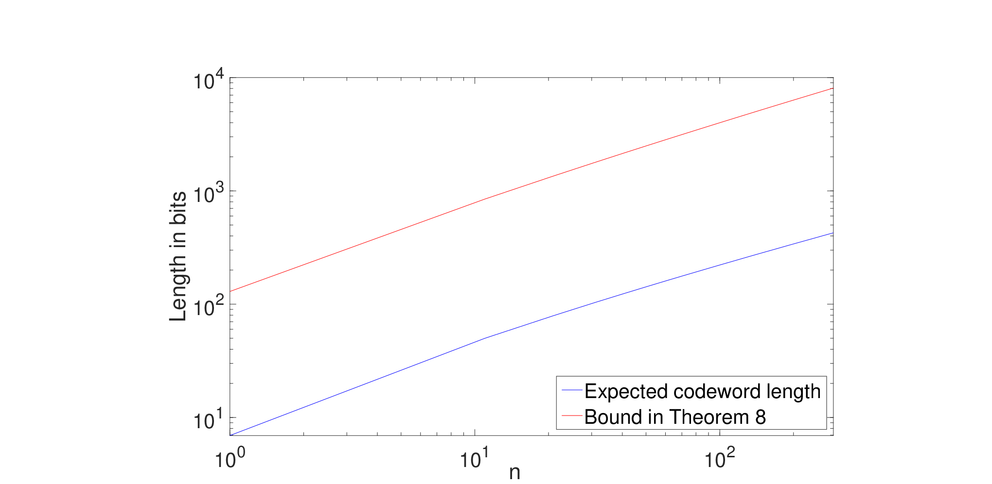
Figure 2 depicts the decomposition of this pdf into rectangles. Figure 3 depicts a log-log plot of the expected codeword length (computed by listing all rectangles with width at least 2−82^{-8}) versus nn, compared to the bound in Theorem 8. Notice that the growth rate of the expected codeword length has a similar order as our bound, and they are both sublinear (which can be observed from their slopes in the log-log plot which are less than 11).

Refer to caption
Figure 2: Decomposition of the distribution in Example 9.
Refer to caption
Figure 3: Log-log plot of the expected codeword length and the bound in Theorem 8 for Example 9.

We now prove Theorem 8.

Proof:

Let Nk,a=|R⁡(k,a)∩{p1,p2,…,pn}|N_{k,a}=|R(k,a)\cap\{p_{1},p_{2},\ldots,p_{n}\}|. Since nn points are generated randomly and independently on the hyp​f+\mathrm{hyp}f^{+}, Nk,aN_{k,a} is a random variable and follows a distribution Binomial⁡(n,A⁡(k,a))\mathrm{Binomial}(n,A(k,a)), where A⁡(k,a)A(k,a) is the area of rectangle R⁡(k,a)R(k,a). More specifically, A⁡(k,a)=2−k​(f⁡(2−k​(2​a+1))−f⁡(2−k+1​(a+1)))A(k,a)=2^{-k}\left(f\left(2^{-k}(2a+1)\right)-f\left(2^{-k+1}(a+1)\right)\right). Also, the probability to include the triple (k,a,Nk,a)(k,a,N_{k,a}) in the encoding WW is equal to 𝐏⁡(Nk,a≥1)\mathbf{P}(N_{k,a}\geq 1). The expected codeword length 𝐄⁡[L⁡(W)]\mathbf{E}\left[L(W)\right] can be calculated by summing the expected codeword length for all possible triples.

𝐄⁡[L⁡(W)]\displaystyle\mathbf{E}\left[L(W)\right]
=∑k=0∞∑a=0max⁡(2k−1−1,0)(L⁡(gs​(k))+L⁡(gs​(a)))​𝐏​(Nk,a≥1)\displaystyle=\sum_{k=0}^{\infty}\sum_{a=0}^{\max(2^{k-1}-1,0)}\left(L\left(g_{s}(k)\right)+L\left(g_{s}(a)\right)\right)\mathbf{P}(N_{k,a}\geq 1)
+∑k=0∞∑a=0max⁡(2k−1−1,0)𝐄[L(g(Nk,a))]\displaystyle\ \ \ \ +\sum_{k=0}^{\infty}\sum_{a=0}^{\max(2^{k-1}-1,0)}\mathbf{E}\left[L\left(g(N_{k,a})\right)\right]
=(L⁡(gs​(0))+L⁡(gs​(0)))​𝐏​(N0,0≥1)\displaystyle=\left(L\left(g_{s}(0)\right)+L\left(g_{s}(0)\right)\right)\mathbf{P}(N_{0,0}\geq 1)
+∑k=1∞∑a=02k−1−1(L(gs(k)))(1−(1−A(k,a)))n\displaystyle\ \ \ \ +\sum_{k=1}^{\infty}\sum_{a=0}^{2^{k-1}-1}\left(L\left(g_{s}(k)\right)\right)\left(1-\left(1-A(k,a)\right){}^{n}\right)
+∑k=1∞∑a=02k−1−1(L(gs(a)))(1−(1−A(k,a)))n\displaystyle\ \ \ \ +\sum_{k=1}^{\infty}\sum_{a=0}^{2^{k-1}-1}\left(L\left(g_{s}(a)\right)\right)\left(1-\left(1-A(k,a)\right){}^{n}\right)
+𝐄⁡[L⁡(g⁡(N0,0))]\displaystyle\ \ \ \ +\mathbf{E}\left[L(g(N_{0,0}))\right]
+∑k=1∞∑a=02k−1−1𝐄[L(g(Nk,a))].\displaystyle\ \ \ \ +\sum_{k=1}^{\infty}\sum_{a=0}^{2^{k-1}-1}\mathbf{E}\left[L\left(g(N_{k,a})\right)\right]. (6)

Note that (L⁡(gs​(0))+L⁡(gs​(0)))​𝐏​(N0,0≥1)≤(1+1)​(1)=2\left(L\left(g_{s}(0)\right)+L\left(g_{s}(0)\right)\right)\mathbf{P}(N_{0,0}\geq 1)\leq(1+1)(1)=2.

Consider the term 1−(1−A(k,a))n1-\left(1-A(k,a)\right){}^{n} in (6). Let k0=⌊log⁡(n​f​(0)+1)⌋k_{0}=\left\lfloor\log\left(\sqrt{nf(0)}+1\right)\right\rfloor. If k≤k0k\leq k_{0}, then bound 1−(1−A⁡(k,a))n1-(1-A(k,a))^{n} above by 1. Otherwise, bound 1−(1−A⁡(k,a))n1-(1-A(k,a))^{n} above by n​A​(k,a)nA(k,a). Consider the term ∑k=1∞∑a=02k−1−1(L(gs(k))+L(gs(a)))(1−(1−A(k,a)))n,\sum_{k=1}^{\infty}\sum_{a=0}^{2^{k-1}-1}\left(L\left(g_{s}(k)\right)+L\left(g_{s}(a)\right)\right)\left(1-\left(1-A(k,a)\right){}^{n}\right), we have

∑k=1∞∑a=02k−1−1(L(gs(k))+L(gs(a)))(1−(1−A(k,a)))n\displaystyle\sum_{k=1}^{\infty}\sum_{a=0}^{2^{k-1}-1}\left(L\left(g_{s}(k)\right)+L\left(g_{s}(a)\right)\right)\left(1-\left(1-A(k,a)\right){}^{n}\right)
≤∑k=1k0∑a=02k−1−1(L⁡(gs​(k))+L⁡(gs​(a)))\displaystyle\leq\sum_{k=1}^{k_{0}}\sum_{a=0}^{2^{k-1}-1}\left(L\left(g_{s}(k)\right)+L\left(g_{s}(a)\right)\right)
+∑k=k0+1∞∑a=02k−1−1(L(gs(k))+L(gs(a)))nA(k,a).\displaystyle\ \ \ \ +\sum_{k=k_{0}+1}^{\infty}\sum_{a=0}^{2^{k-1}-1}\left(L\left(g_{s}(k)\right)+L\left(g_{s}(a)\right)\right)nA(k,a).

Consider the term ∑k=1k0∑a=02k−1−1L⁡(gs​(k))\sum_{k=1}^{k_{0}}\sum_{a=0}^{2^{k-1}-1}L\left(g_{s}(k)\right) in (6). We have

∑k=1k0∑a=02k−1−1L⁡(gs​(k))\displaystyle\sum_{k=1}^{k_{0}}\sum_{a=0}^{2^{k-1}-1}L\left(g_{s}(k)\right)
≤∑k=1k02k​log⁡(2​k+3)\displaystyle\leq\sum_{k=1}^{k_{0}}2^{k}\log(2k+3)
≤∑k=1k0(k+1)​(2k+1)\displaystyle\mathrel{{\mathop{\leq}\limits}}\sum_{k=1}^{k_{0}}(k+1)(2^{k+1})
=2k0+2​k0\displaystyle=2^{k_{0}+2}k_{0}
≤4​(n​f​(0)+1)​log⁡(n​f​(0)+1)\displaystyle\leq 4(\sqrt{nf(0)}+1)\log(\sqrt{nf(0)}+1)
≤8​n​f​(0)​log⁡(n​f​(0)+1),\displaystyle\leq 8\sqrt{nf(0)}\log(\sqrt{nf(0)}+1),

where (a)(a) follows from the fact that log⁡(2​k+3)≤2​k+2\log(2k+3)\leq 2k+2 when k≥1k\geq 1.

Consider the term ∑k=1k0∑a=02k−1−1L⁡(gs​(a))\sum_{k=1}^{k_{0}}\sum_{a=0}^{2^{k-1}-1}L\left(g_{s}(a)\right) in (6). We have

∑k=1k0∑a=02k−1−1L⁡(gs​(a))\displaystyle\sum_{k=1}^{k_{0}}\sum_{a=0}^{2^{k-1}-1}L\left(g_{s}(a)\right)
≤∑k=1k0∑a=02k−1−12​log⁡(2​a+3)\displaystyle\leq\sum_{k=1}^{k_{0}}\sum_{a=0}^{2^{k-1}-1}2\log(2a+3)
≤∑k=1k0∫02k−12​log⁡(2​a+3)​𝑑a\displaystyle\leq\sum_{k=1}^{k_{0}}\int_{0}^{2^{k-1}}2\log(2a+3)da
=∑k=1k0(2k+3)​log⁡(2k+3)−3​log⁡3−2k\displaystyle=\sum_{k=1}^{k_{0}}(2^{k}+3)\log(2^{k}+3)-3\log 3-2^{k}
≤∑k=1k02k​log⁡(2k+2)\displaystyle\leq\sum_{k=1}^{k_{0}}2^{k}\log(2^{k+2})
=∑k=1k0(k+2)​2k\displaystyle=\sum_{k=1}^{k_{0}}(k+2)2^{k}
=2​(2k0​k0+2k0−1)\displaystyle=2(2^{k_{0}}k_{0}+2^{k_{0}}-1)
≤4​(n​f​(0)+1)​log⁡(n​f​(0)+1)\displaystyle\leq 4(\sqrt{nf(0)}+1)\log(\sqrt{nf(0)}+1)
≤8​n​f​(0)​log⁡(n​f​(0)+1).\displaystyle\leq 8\sqrt{nf(0)}\log(\sqrt{nf(0)}+1).

Consider the term ∑k=k0+1∞∑a=02k−1−1gs​(k)​n​A​(k,a)\sum_{k=k_{0}+1}^{\infty}\sum_{a=0}^{2^{k-1}-1}g_{s}(k)nA(k,a) in (6). We have

∑k=k0+1∞∑a=02k−1−1gs​(k)​n​A​(k,a)\displaystyle\sum_{k=k_{0}+1}^{\infty}\sum_{a=0}^{2^{k-1}-1}g_{s}(k)nA(k,a)
≤n∑k=k0+1∞∑a=02k−1−1log(2k+3)2−k+1[f(2−k(2a+1))\displaystyle\leq n\sum_{k=k_{0}+1}^{\infty}\sum_{a=0}^{2^{k-1}-1}\log(2k+3)2^{-k+1}\left[f\left(2^{-k}(2a+1)\right)\right.
−f(2−k+1(a+1))]\displaystyle\ \ \ \ \left.-f\left(2^{-k+1}(a+1)\right)\right]
≤n​∑k=k0+1∞log⁡(2​k+3)​2−k+1​f​(0)\displaystyle\mathrel{{\mathop{\leq}\limits}}n\sum_{k=k_{0}+1}^{\infty}\log(2k+3)2^{-k+1}f(0)
≤(c)​n​f​(0)​∑k=k0+1∞(k+1)​2−k+1\displaystyle\overset{(c)}{\leq}nf(0)\sum_{k=k_{0}+1}^{\infty}(k+1)2^{-k+1}
=n​f​(0)​2−k0+1​(k0+3)\displaystyle=nf(0)2^{-k_{0}+1}(k_{0}+3)
≤n​f​(0)​2−k0+3​k0\displaystyle\leq nf(0)2^{-k_{0}+3}k_{0}
≤n​f​(0)​24−log⁡(n​f​(0)+1)​log⁡(n​f​(0)+1)\displaystyle\leq nf(0)2^{4-\log\left(\sqrt{nf(0)}+1\right)}\log\left(\sqrt{nf(0)}+1\right)
=16​n​f​(0)n​f​(0)+1​log⁡(n​f​(0)+1)\displaystyle=\dfrac{16nf(0)}{\sqrt{nf(0)}+1}\log(\sqrt{nf(0)}+1)
≤16​n​f​(0)​log⁡(n​f​(0)+1),\displaystyle\leq 16\sqrt{nf(0)}\log(\sqrt{nf(0)}+1),

where (b)(b) follow by the fact that ∑a=02k−1−1f⁡(2−k​(2​a+1))−f⁡(2−k+1​(a+1))≤f⁡(2−k)≤f⁡(0).\sum_{a=0}^{2^{k-1}-1}f\left(2^{-k}(2a+1)\right)-f\left(2^{-k+1}(a+1)\right)\leq f(2^{-k})\leq f(0). For (c)(c), k+1≥log⁡(2​k+3)k+1\geq\log(2k+3), when k≥2k\geq 2.

Consider the term ∑k=k0+1∞∑a=02k−1−1gs​(a)​n​A​(k,a)\sum_{k=k_{0}+1}^{\infty}\sum_{a=0}^{2^{k-1}-1}g_{s}(a)nA(k,a) in (6). We have

∑k=k0+1∞∑a=02k−1−1gs​(a)​n​A​(k,a)\displaystyle\sum_{k=k_{0}+1}^{\infty}\sum_{a=0}^{2^{k-1}-1}g_{s}(a)nA(k,a)
=n​∑k=k0+1∞∑a=02k−1−1log⁡(2​a+3)​21−k​(f⁡(2−k​(2​a+1))CLOSE\displaystyle=n\sum_{k=k_{0}+1}^{\infty}\sum_{a=0}^{2^{k-1}-1}\log(2a+3)2^{1-k}\Big(f\left(2^{-k}(2a+1)\right)
OPEN−f⁡(2−k+1​(a+1)))\displaystyle\ \ \ \ -f\left(2^{-k+1}(a+1)\right)\Big)
≤n​∑k=k0+1∞∑a=02k−1−1log⁡(2k+1)​21−k​(f⁡(2−k​(2​a+1)CLOSECLOSE\displaystyle\mathrel{{\mathop{\leq}\limits}}n\sum_{k=k_{0}+1}^{\infty}\sum_{a=0}^{2^{k-1}-1}\log(2^{k+1})2^{1-k}\Big(f\left(2^{-k}(2a+1\right)
OPEN−f⁡(2−k+1​(a+1)))\displaystyle\ \ \ \ -f\left(2^{-k+1}(a+1)\right)\Big)
≤n​f​(0)​∑k=k0+1∞(k+1)​21−k\displaystyle\leq nf(0)\sum_{k=k_{0}+1}^{\infty}\left(k+1\right)2^{1-k}
≤16​n​f​(0)​log⁡(n​f​(0)+1),\displaystyle\leq 16\sqrt{nf(0)}\log(\sqrt{nf(0)}+1),

where (d)(d) follows from the fact that log⁡(2​a+3)≤log⁡(2k+1)≤log⁡(2k+1)\log(2a+3)\leq\log(2^{k}+1)\leq\log(2^{k+1}) for aa∈[0:2k−1−1]\in\left[0:2^{k-1}-1\right].

Consider the term 𝐄⁡[L⁡(g⁡(N0,0))]\mathbf{E}\left[L(g(N_{0,0}))\right] in (6). We have

𝐄⁡[L⁡(g⁡(N0,0))]\displaystyle\mathbf{E}\left[L(g(N_{0,0}))\right]
≤𝐄⁡(2​log⁡(2​N0,0+1))\displaystyle\leq\mathbf{E}(2\log(2N_{0,0}+1))
≤(e)​2​log⁡(2​𝐄​(N0,0)+1)\displaystyle\overset{(e)}{\leq}2\log(2\mathbf{E}(N_{0,0})+1)
=2​log⁡(2​n​f​(1)+1)\displaystyle=2\log(2nf(1)+1)
≤2​log⁡(3​n​f​(0))\displaystyle\leq 2\log(3nf(0))
≤4+4​log⁡(n​f​(0)+1),\displaystyle\leq 4+4\log(\sqrt{nf(0)}+1),

where (e)(e) follows from Jensen’s inequality.

Consider the term ∑k=1∞∑a=02k−1−1𝐄⁡[L⁡(g⁡(Nk,a))]\sum_{k=1}^{\infty}\sum_{a=0}^{2^{k-1}-1}\mathbf{E}\left[L\left(g(N_{k,a})\right)\right] in (6). We have

∑k=1∞∑a=02k−1−1𝐄⁡[L⁡(g⁡(Nk,a))]\displaystyle\sum_{k=1}^{\infty}\sum_{a=0}^{2^{k-1}-1}\mathbf{E}\left[L\left(g(N_{k,a})\right)\right]
≤∑k=1∞∑a=02k−1−1𝐄⁡[2​log⁡(2​Nk,a+1)]\displaystyle\leq\sum_{k=1}^{\infty}\sum_{a=0}^{2^{k-1}-1}\mathbf{E}\left[2\log\left(2N_{k,a}+1\right)\right]
≤∑k=1∞∑a=02k−1−12​log⁡(2​𝐄​(Nk,a)+1)\displaystyle\mathrel{{\mathop{\leq}\limits}}\sum_{k=1}^{\infty}\sum_{a=0}^{2^{k-1}-1}2\log(2\mathbf{E}(N_{k,a})+1)
=∑k=1∞∑a=02k−1−12​log⁡(2​n​A​(k,a)+1)\displaystyle=\sum_{k=1}^{\infty}\sum_{a=0}^{2^{k-1}-1}2\log(2nA(k,a)+1)
=∑k=1∞∑a=02k−1−12​log⁡(CLOSE\displaystyle=\sum_{k=1}^{\infty}\sum_{a=0}^{2^{k-1}-1}2\log\Big(
OPEN2​n​(2−k​(f⁡(2−k​(2​a+1))−f⁡(2−k+1​(a+1))))+1)\displaystyle\ \ \ \ 2n\left(2^{-k}\left(f\left(2^{-k}(2a+1)\right)-f\left(2^{-k+1}(a+1)\right)\right)\right)+1\Big)
≤(g)​∑k=1∞2k​log⁡(CLOSE\displaystyle\overset{(g)}{\leq}\sum_{k=1}^{\infty}2^{k}\log\bigg(
OPEN4​n22​k​∑a=02k−1−1[f⁡(2−k​(2​a+1))−f⁡(2−k+1​(a+1))]+1)\displaystyle\ \ \ \ \dfrac{4n}{2^{2k}}\sum_{a=0}^{2^{k-1}-1}\left[f\left(2^{-k}(2a+1)\right)-f\left(2^{-k+1}(a+1)\right)\right]+1\bigg)
≤∑k=1∞2k​log⁡(4​n​f​(0)22​k+1),\displaystyle\leq\sum_{k=1}^{\infty}2^{k}\log\left(\dfrac{4nf(0)}{2^{2k}}+1\right),

where (f)(f)and (g)(g) follows by Jensen’s inequality.

Let k1=⌊log(4​n​f​(0)⌋k_{1}=\left\lfloor\log(\sqrt{4nf(0)}\right\rfloor. We have

∑k=1∞2k​log⁡(4​n​f​(0)22​k+1)\displaystyle\sum_{k=1}^{\infty}2^{k}\log\left(\dfrac{4nf(0)}{2^{2k}}+1\right)
=∑k=1k12k​log⁡(4​n​f​(0)22​k+1)\displaystyle=\sum_{k=1}^{k_{1}}2^{k}\log\left(\dfrac{4nf(0)}{2^{2k}}+1\right)
+∑k=k1+1∞2klog(4​n​f​(0)22​k+1)\displaystyle\ \ \ \ +\sum_{k=k_{1}+1}^{\infty}2^{k}\log\left(\dfrac{4nf(0)}{2^{2k}}+1\right)
≤(h)​∑k=1k12k​log⁡(8​n​f​(0)22​k)+∫k1∞2k​log⁡(4​n​f​(0)22​k+1)​𝑑k,\displaystyle\overset{(h)}{\leq}\sum_{k=1}^{k_{1}}2^{k}\log\left(\dfrac{8nf(0)}{2^{2k}}\right)+\int_{k_{1}}^{\infty}2^{k}\log\left(\dfrac{4nf(0)}{2^{2k}}+1\right)dk, (7)

where (h)(h) follows from the fact that 4​n​f​(0)22​k≥1\dfrac{4nf(0)}{2^{2k}}\geq 1 when k≤k1k\leq k_{1} and 2k​log⁡(4​n​f​(0)22​k+1)2^{k}\log\left(\dfrac{4nf(0)}{2^{2k}}+1\right) is decreasing when k≥k1+1k\geq k_{1}+1.

Consider the term ∑k=1k12k​log⁡(8​n​f​(0)22​k)\sum_{k=1}^{k_{1}}2^{k}\log\left(\dfrac{8nf(0)}{2^{2k}}\right) in (7),

∑k=1k12k​log⁡(8​n​f​(0)22​k)\displaystyle\sum_{k=1}^{k_{1}}2^{k}\log\left(\dfrac{8nf(0)}{2^{2k}}\right)
=2​(2k1−1)​log⁡(8​n​f​(0))−4​(2k1​k1−2k1+1)\displaystyle=2(2^{k_{1}}-1)\log(8nf(0))-4(2^{k_{1}}k_{1}-2^{k_{1}}+1)
≤2k1+1​log⁡(8​n​f​(0))−4​(2k1​k1−2k1)\displaystyle\leq 2^{k_{1}+1}\log(8nf(0))-4(2^{k_{1}}k_{1}-2^{k_{1}})
≤(i)​20​n​f​(0)+4​n​f​(0)​log⁡(n​f​(0))\displaystyle\overset{(i)}{\leq}20\sqrt{nf(0)}+4\sqrt{nf(0)}\log(\sqrt{nf(0)})
≤24​n​f​(0)​log⁡(n​f​(0)+1),\displaystyle\leq 24\sqrt{nf(0)}\log(\sqrt{nf(0)}+1),

where (i)(i) follows from the fact that log⁡(4​n​f​(0))−1≤k1≤log⁡(4​n​f​(0)CLOSE\log(\sqrt{4nf(0)})-1\leq k_{1}\leq\log(\sqrt{4nf(0)}, and thus n​f​(0)≤2k1≤2​n​f​(0).\sqrt{nf(0)}\leq 2^{k_{1}}\leq 2\sqrt{nf(0)}.

Consider the term ∫k1∞2k​log⁡(4​n​f​(0)22​k+1)​𝑑k\int_{k_{1}}^{\infty}2^{k}\log\left(\dfrac{4nf(0)}{2^{2k}}+1\right)dk in (7),

∫k1∞2k​log⁡(4​n​f​(0)22​k+1)​𝑑k\displaystyle\int_{k_{1}}^{\infty}2^{k}\log\left(\dfrac{4nf(0)}{2^{2k}}+1\right)dk
=2​log2⁡e​4​n​f​(0)​arctan⁡(4​n​f​(0)2k1)\displaystyle=2\log^{2}e\sqrt{4nf(0)}\arctan\left(\frac{\sqrt{4nf(0)}}{2^{k_{1}}}\right)
−2k1​log⁡(22​k1+4​n​f​(0)22​k1)​log​e\displaystyle\ \ \ \ -2^{k_{1}}\log\left(\frac{2^{2k_{1}}+4nf(0)}{2^{2k_{1}}}\right)\log e
≤4​n​f​(0)​arctan⁡(2)​log2​e\displaystyle\leq 4\sqrt{nf(0)}\arctan(2)\log^{2}e
≤10​n​f​(0).\displaystyle\leq 10\sqrt{nf(0)}.

Therefore,

𝐄⁡[L⁡(W)]\displaystyle\mathbf{E}\left[L(W)\right]
≤72​n​f​(0)​(log⁡(n​f​(0)+1))+10​n​f​(0)\displaystyle\leq 72\sqrt{nf(0)}(\log(\sqrt{nf(0)}+1))+10\sqrt{nf(0)}
+4+4​log⁡(n​f​(0)+1)+2\displaystyle\ \ \ \ +4+4\log(\sqrt{nf(0)}+1)+2
≤92​n​f​(0)​(log⁡(n​f​(0)+1)).\displaystyle\leq 92\sqrt{nf(0)}(\log(\sqrt{nf(0)}+1)).

∎

IV PP is a distribution over [0,∞)[0,\infty) with a non-increasing pdf

With the previous two coding schemes as our building blocks, we can develop a coding scheme for the case where PP is a continuous distribution over [0,∞)\left[0,\infty\right) with a non-increasing pdf ff based on the dyadic decomposition construction in [8, 9]. If PP satisfy a power law bound, we show the growth rate of expected codeword length is sub-linear.

Definition 10.

The coding scheme for the case where PP is a distribution over [0,∞)[0,\infty) with a non-increasing pdf consists of:

  1. 1.

    Encoder:

    1. (a)

      After the encoder observes PP, it generates i.i.d. X~1,X~2,…,X~n∼P\widetilde{X}_{1},\widetilde{X}_{2},...,\widetilde{X}_{n}\sim P.

    2. (b)

      Apply the difference run-length encoding scheme in Definition 2 to encode ⌈X~1⌉,…,⌈X~n⌉\lceil\widetilde{X}_{1}\rceil,\ldots,\lceil\widetilde{X}_{n}\rceil. Let its output be Wint∈{0,1}∗W_{\mathrm{int}}\in\{0,1\}^{*}.

    3. (c)

      Let ni=|{j:X~j∈[i−1,i)}|n_{i}=|\{j:\widetilde{X}_{j}\in[i-1,i)\}|. For each positive integer ii where ni>0n_{i}>0, apply the scheme in Definition 7 to generate nin_{i} points with pdf

      fi​(x)=f⁡(x+i−1)∫i−1if⁡(t)​𝑑t.f_{i}(x)=\frac{f(x+i-1)}{\int_{i-1}^{i}f(t)dt}.

      Let its output be Wi∈{0,1}∗W_{i}\in\{0,1\}^{*}. For ii where ni=0n_{i}=0, let Wi=∅W_{i}=\emptyset.

    4. (d)

      The encoder outputs W=Wint​‖W1‖​W2|⋯W=W_{\mathrm{int}}\|W_{1}\|W_{2}\|\cdots.

  2. 2.

    Decoder:

    1. (a)

      Upon receiving WW, the decoder decodes WintW_{\mathrm{int}} and recovers the multiset {⌈X~1⌉,…,⌈X~n⌉}\{\lceil\widetilde{X}_{1}\rceil,\ldots,\lceil\widetilde{X}_{n}\rceil\}, and hence recovers nin_{i} for nonnegative integers ii.

    2. (b)

      For each ii where ni>0n_{i}>0, the decoder decodes WiW_{i} using WW, and use the decoding scheme in Definition 7 to generate i.i.d. Xi,1,…,Xi,ni∼fiX_{i,1},\ldots,X_{i,n_{i}}\sim f_{i}.

    3. (c)

      The decoder randomly shuffles {Xi,j}i≥1,j∈[1:ni]\{X_{i,j}\}_{i\geq 1,\,j\in[1:n_{i}]} and output the shuffled sequence.

We present the following theorem which shows that the codeword length grows sub-linearly in nn when PP follows a non-increasing pdf and satisfies a power law bound.

Theorem 11.

The expected codeword length of the above coding scheme, for the case where PP is a distribution over [0,∞)[0,\infty) with a non-increasing pdf, and PP satisfies the bound 𝐏⁡(X>x)≤c​x−λ\text{$\mathbf{P}$}(X>x)\leq cx^{-\lambda} for all x∈[0,∞)x\in[0,\infty), where c>1c>1 and λ>1\lambda>1, is bounded above as

𝐄⁡(L⁡(W))\displaystyle\mathbf{E}\left(L\left(W\right)\right) ≤418​c​(λ+1)​max⁡(n1/λ,n)​max⁡(f⁡(0),1)min⁡(λ−1,1)\displaystyle\leq\dfrac{418c(\lambda+1)\max(n^{1/\lambda},\sqrt{n})\max(\sqrt{f(0)},1)}{\min(\lambda-1,1)}
⋅log⁡(n​max⁡(f⁡(0),1)+1).\displaystyle\ \ \ \ \cdot\log(\sqrt{n\max(f(0),1)}+1).

Before proving the theorem, we review the concept of majorization for non-increasing functions [14].

Definition 12 (Majorization).

Let f,gf,g be two continuous non-increasing functions over [0,∞)[0,\infty). It is said that ff is majorized by gg, denoted by f≺gf\prec g, if ∫0xf⁡(t)​𝑑t≤∫0xg⁡(t)​𝑑t\int_{0}^{x}f(t)dt\leq\int_{0}^{x}g(t)dt for any x≥0x\geq 0.

We state the following equivalent characterization of majorization, which is proved in [14, Theorem 2.5].

Lemma 13 ([14]).

Let f,gf,g be two continuous functions. f≺gf\prec g if and only if

∫0∞ϕ⁡(f⁡(t))​𝑑t\displaystyle\int_{0}^{\infty}\phi(f(t))dt ≥∫0∞ϕ⁡(g⁡(t))​𝑑t\displaystyle\geq\int_{0}^{\infty}\phi(g(t))dt

for all concave function ϕ:ℝ→ℝ.\phi:\mathbb{R\rightarrow\mathbb{R}}.

Before we prove Theorem 11, we show the following lemma.

Lemma 14.

Let ff be a non-increasing pdf over [0,∞)[0,\infty) that satisfies the bound ∫x∞f⁡(t)​𝑑t≤c​x−λ\int_{x}^{\infty}f(t)dt\leq cx^{-\lambda} for any x∈[0,∞)x\in[0,\infty). Let f∗:[0,∞)→ℝf^{*}:[0,\infty)\rightarrow\mathbb{R} be a pdf defined as

f∗​(x)=\displaystyle f^{*}(x)= {c​λ​t0−λ−1,x≤t0c​λ​x−λ−1,x>t0,\displaystyle\begin{cases}c\lambda t_{0}^{-\lambda-1}&,x\leq t_{0}\\ c\lambda x^{-\lambda-1}&,x>t_{0},\end{cases}

where t0=(c⁡(λ+1))1/λt_{0}=\left(c(\lambda+1)\right)^{1/\lambda}. Then f≻f∗.f\succ f^{*}.

Proof:

Note that ∫0∞f∗​(x)​𝑑x=1.\int_{0}^{\infty}f^{*}(x)dx=1. Further note that f⁡(0)≥f∗​(0),f(0)\geq f^{*}(0),otherwise ∫0∞f⁡(x)​𝑑x<∫0∞f∗​(x)​𝑑x=1.\int_{0}^{\infty}f(x)dx<\int_{0}^{\infty}f^{*}(x)dx=1. Suppose ∫0af⁡(x)​𝑑x<∫0af∗​(x)​𝑑x\int_{0}^{a}f(x)dx<\int_{0}^{a}f^{*}(x)dx for some aa. Suppose a≤t0.a\leq t_{0}. Note that f​(a)<f∗​(a)f(a)<f^{*}(a) and thus f​(x)<f∗​(x)f(x)<f^{*}(x) when x≥ax\geq a. Thus, ∫0∞f⁡(x)​𝑑x=∫0af⁡(x)​𝑑x+∫a∞f⁡(x)​𝑑x<∫0af∗​(x)​𝑑x+∫a∞f∗​(x)​𝑑x=1.\int_{0}^{\infty}f(x)dx=\int_{0}^{a}f(x)dx+\int_{a}^{\infty}f(x)dx<\int_{0}^{a}f^{*}(x)dx+\int_{a}^{\infty}f^{*}(x)dx=1. Contradiction arises. Suppose a>t0.a>t_{0}. Note that ∫a∞f⁡(x)​𝑑x≤c​a−λ=∫a∞f∗​(x)​𝑑x\int_{a}^{\infty}f(x)dx\leq ca^{-\lambda}=\int_{a}^{\infty}f^{*}(x)dx. Thus, ∫0∞f⁡(x)​𝑑x=∫0af⁡(x)​𝑑x+∫a∞f⁡(x)​𝑑x<∫0af∗​(x)​𝑑x+∫a∞f∗​(x)​𝑑x=1.\int_{0}^{\infty}f(x)dx=\int_{0}^{a}f(x)dx+\int_{a}^{\infty}f(x)dx<\int_{0}^{a}f^{*}(x)dx+\int_{a}^{\infty}f^{*}(x)dx=1. Contradiction arises. Therefore, f≻f∗f\succ f^{*}. ∎We now present the proof of Theorem 11.

Proof:

Let ff be the pdf of the distribution PP, and XX be a random variable following the distribution of PP. Consider the distribution of ⌈X⌉\lceil X\rceil. We have, for integer x≥0x\geq 0,

𝐏⁡(⌈X⌉>x)\displaystyle\mathbf{P}(\lceil X\rceil>x) =𝐏⁡(X>x)\displaystyle=\mathbf{P}\left(X>x\right)
≤c​x−λ.\displaystyle\leq cx^{-\lambda}.

By Theorem 4, we have

𝐄⁡(L⁡(Wint))≤50​c​λ​n1λ​log⁡(n+1)λ−1.\mathbf{E}(L(W_{\mathrm{int}}))\leq\dfrac{50c\lambda n^{\frac{1}{\lambda}}\log(\sqrt{n}+1)}{\lambda-1}.

Consider WiW_{i} for i≥1i\geq 1. By Theorem 8,

𝐄⁡(L⁡(Wi))\displaystyle\mathbf{E}(L(W_{i}))
≤𝐄(𝟏{ni≥1}⋅92ni​fi​(0)(log(ni​fi​(0)+1)))\displaystyle\leq\mathbf{E}\left(\mathbf{1}\{n_{i}\geq 1\}\cdot 92\sqrt{n_{i}f_{i}(0)}(\log(\sqrt{n_{i}f_{i}(0)}+1))\right)
=𝐄⁡(92​ni​fi​(0)​(log⁡(ni​fi​(0)+1)))\displaystyle=\mathbf{E}\left(92\sqrt{n_{i}f_{i}(0)}(\log(\sqrt{n_{i}f_{i}(0)}+1))\right)
≤(a)​92​𝐄⁡(ni)​fi​(0)​(log⁡(𝐄⁡(ni)​fi​(0)+1))\displaystyle\overset{(a)}{\leq}92\sqrt{\mathbf{E}(n_{i})f_{i}(0)}(\log(\sqrt{\mathbf{E}(n_{i})f_{i}(0)}+1))
=(b)​92​n​f​(i−1)​(log⁡(n​f​(i−1)+1)),\displaystyle\overset{(b)}{=}92\sqrt{nf(i-1)}(\log(\sqrt{nf(i-1)}+1)),

where (a)(a) is by Jensen’s inequality and the concavity of t​log⁡(t+1)\sqrt{t}\log(\sqrt{t}+1), and (b)(b) is by

𝐄⁡(ni)​fi​(0)\displaystyle\mathbf{E}(n_{i})f_{i}(0) =(n​∫i−1if⁡(t)​𝑑t)​f⁡(i−1)∫i−1if⁡(t)​𝑑t\displaystyle=\left(n\int_{i-1}^{i}f(t)dt\right)\frac{f(i-1)}{\int_{i-1}^{i}f(t)dt}
=n​f​(i−1).\displaystyle=nf(i-1).

Hence, we have

∑i=1∞𝐄⁡(L⁡(Wi))\displaystyle\sum_{i=1}^{\infty}\mathbf{E}(L(W_{i}))
≤∑i=1∞92​n​f​(i−1)​(log⁡(n​f​(i−1)+1))\displaystyle\leq\sum_{i=1}^{\infty}92\sqrt{nf(i-1)}(\log(\sqrt{nf(i-1)}+1))
≤92​n​f​(0)​(log⁡(n​f​(0)+1)CLOSE\displaystyle\leq 92\sqrt{nf(0)}(\log(\sqrt{nf(0)}+1)
+∫0∞92n​f​(x)(log(n​f​(x)+1))dx.\displaystyle\ \ \ \ +\int_{0}^{\infty}92\sqrt{nf(x)}\left(\log(\sqrt{nf(x)}+1)\right)dx.

Consider the term ∫0∞72​n​f​(x)​(log⁡(n​f​(x)+1))​𝑑x\int_{0}^{\infty}72\sqrt{nf(x)}\left(\log(\sqrt{nf(x)}+1)\right)dx. By Lemma 13, Lemma 14 and the concavity of t​log⁡(t+1)\sqrt{t}\log(\sqrt{t}+1),

∫0∞92​n​f​(x)​(log⁡(n​f​(x)+1))​𝑑x\displaystyle\int_{0}^{\infty}92\sqrt{nf(x)}\left(\log(\sqrt{nf(x)}+1)\right)dx
≤∫0∞92​n​f∗​(x)​(log⁡(n​f∗​(x)+1))​𝑑x\displaystyle\leq\int_{0}^{\infty}92\sqrt{nf^{*}(x)}\left(\log(\sqrt{nf^{*}(x)}+1)\right)dx
=∫0t092​n​f∗​(x)​(log⁡(n​f∗​(x)+1))​𝑑x\displaystyle=\int_{0}^{t_{0}}92\sqrt{nf^{*}(x)}\left(\log(\sqrt{nf^{*}(x)}+1)\right)dx
+∫t0∞92n​f∗​(x)(log(n​f∗​(x)+1))dx\displaystyle\ \ \ \ +\int_{t_{0}}^{\infty}92\sqrt{nf^{*}(x)}\left(\log(\sqrt{nf^{*}(x)}+1)\right)dx
≤92​t0​n​f∗​(0)​(log⁡(n​f∗​(0)+1)CLOSE\displaystyle\leq 92t_{0}\sqrt{nf^{*}(0)}\left(\log(\sqrt{nf^{*}(0)}+1\right)
+92∫t0∞n​c​λ​x−λ−1(log(n​f∗​(0)+1))dx\displaystyle\ \ \ \ +92\int_{t_{0}}^{\infty}\sqrt{nc\lambda x^{-\lambda-1}}\left(\log(\sqrt{nf^{*}(0)}+1)\right)dx
≤(c)​92​t0​n​(log⁡(n+1)CLOSE\displaystyle\overset{(c)}{\leq}92t_{0}\sqrt{n}\left(\log(\sqrt{n}+1\right)
+92∫t0∞n​c​λ​x−λ−1(log(n+1))dx\displaystyle\ \ \ \ +92\int_{t_{0}}^{\infty}\sqrt{nc\lambda x^{-\lambda-1}}\left(\log(\sqrt{n}+1)\right)dx
=92​(c⁡(λ+1))1λ​n​log⁡(n+1)\displaystyle=92\left(c(\lambda+1)\right)^{\frac{1}{\lambda}}\sqrt{n}\log(\sqrt{n}+1)
+184​n​c​λ​log⁡(n+1)(λ−1)​(c⁡(λ+1))λ−12​λ\displaystyle\ \ \ \ +\frac{184\sqrt{nc\lambda}\log(\sqrt{n}+1)}{(\lambda-1)\left(c(\lambda+1)\right)^{\frac{\lambda-1}{2\lambda}}}
≤92​(c⁡(λ+1))1λ​n​log⁡(n+1)\displaystyle\leq 92\left(c(\lambda+1)\right)^{\frac{1}{\lambda}}\sqrt{n}\log(\sqrt{n}+1)
+184​(c⁡(λ+1))12​λ​n​log⁡(n+1)(λ−1)\displaystyle\ \ \ \ +\frac{184(c(\lambda+1))^{\frac{1}{2\lambda}}\sqrt{n}\log(\sqrt{n}+1)}{(\lambda-1)}
≤276​(c⁡(λ+1))1/λ​n​log⁡(n+1)min⁡(λ−1,1),\displaystyle\leq\frac{276\left(c(\lambda+1)\right)^{1/\lambda}\sqrt{n}\log(\sqrt{n}+1)}{\min(\lambda-1,1)},

where (c)(c) follows from f∗​(0)=c​λ​(c⁡(λ+1))−1−1λ≤1f^{*}(0)=c\lambda\left(c(\lambda+1)\right)^{-1-\frac{1}{\lambda}}\leq 1. Hence,

∑i=1∞𝐄⁡(L⁡(Wi))\displaystyle\sum_{i=1}^{\infty}\mathbf{E}(L(W_{i}))
≤92​n​f​(0)​(log⁡(n​f​(0)+1)CLOSE\displaystyle\leq 92\sqrt{nf(0)}(\log(\sqrt{nf(0)}+1)
+276​(c⁡(λ+1))1/λ​n​log⁡(n+1)min⁡(λ−1,1).\displaystyle\ \ \ \ +\frac{276\left(c(\lambda+1)\right)^{1/\lambda}\sqrt{n}\log(\sqrt{n}+1)}{\min(\lambda-1,1)}.

Therefore, the expected codeword length

𝐄⁡(L⁡(Wint))+∑i=1∞𝐄⁡(L⁡(Wi))\displaystyle\mathbf{E}(L(W_{\mathrm{int}}))+\sum_{i=1}^{\infty}\mathbf{E}(L(W_{i}))
≤50​c​λ​n1λ​log⁡(n+1)λ−1+92​n​f​(0)​(log⁡(n​f​(0)+1)CLOSE\displaystyle\leq\dfrac{50c\lambda n^{\frac{1}{\lambda}}\log(\sqrt{n}+1)}{\lambda-1}+92\sqrt{nf(0)}(\log(\sqrt{nf(0)}+1)
+276​(c⁡(λ+1))1/λ​n​log⁡(n+1)min⁡(λ−1,1)\displaystyle\ \ \ \ +\frac{276\left(c(\lambda+1)\right)^{1/\lambda}\sqrt{n}\log(\sqrt{n}+1)}{\min(\lambda-1,1)}
≤418​c​(λ+1)​max⁡(n1/λ,n)​max⁡(f⁡(0),1)min⁡(λ−1,1)\displaystyle\leq\dfrac{418c(\lambda+1)\max(n^{1/\lambda},\sqrt{n})\max(\sqrt{f(0)},1)}{\min(\lambda-1,1)}
×log⁡(n​max⁡(f⁡(0),1)+1).\displaystyle\ \ \ \ \times\log(\sqrt{n\max(f(0),1)}+1).

Therefore, the expected codeword length grows sublinearly. ∎ Our coding scheme described in Definition 10 uses the coding scheme in Defintion 7 as a building block. Therefore, if we use Theorem 8 in our analysis, then even if we assume a stronger tail bound, such as exponential tail bound 𝐏⁡(X>x)≤c​e−λ​x,\text{$\mathbf{P}$}(X>x)\leq ce^{-\lambda x}, the order of the growth of expected codeword length cannot be better than O​(n​f​(0)​(log⁡(n​f​(0)+1)))O(\sqrt{nf(0)}(\log(\sqrt{nf(0)}+1))).

V Conclusion and Discussion

In this paper, we introduced a new problem in channel simulation called the multiple-output channel simulation. We also describe encoding schemes for three classes of probability distributions and show that the growth rate of the expected codeword length is sub-linear in nn when a power bound or exponential bound is satisfied. An application of multiple-outputs channel simulation is the compression of probability distributions.

We list some potential extenstions of our result. First, it may be possible to generalize the result to more classes of probability distributions, such as unimodal distributions over the real line. Second, since this paper only focus on upper bounds of our codeword length, lower bounds may also be derived in the future in order to show tightness. Third, we may also consider the case where common randomness is available to the encoder and decoder.

VI Acknowledgment

The authors acknowledge support from the Direct Grant for Research, The Chinese University of Hong Kong.

References

  • [1] C. H. Bennett, P. W. Shor, J. A. Smolin, and A. V. Thapliyal, “Entanglement-assisted capacity of a quantum channel and the reverse shannon theorem,” IEEE Transactions on Information Theory, vol. 48, no. 10, pp. 2637–2655, 2002.
  • [2] A. Winter, “Compression of sources of probability distributions and density operators,” arXiv preprint quant-ph/0208131, 2002.
  • [3] P. Cuff, “Distributed channel synthesis,” IEEE Transactions on Information Theory, vol. 59, no. 11, pp. 7071–7096, 2013.
  • [4] P. Harsha, R. Jain, D. McAllester, and J. Radhakrishnan, “The communication complexity of correlation,” in Twenty-Second Annual IEEE Conference on Computational Complexity (CCC’07), pp. 10–23, IEEE, 2007.
  • [5] M. Braverman and A. Garg, “Public vs private coin in bounded-round information,” in International Colloquium on Automata, Languages, and Programming, pp. 502–513, Springer, 2014.
  • [6] C. T. Li and A. El Gamal, “Strong functional representation lemma and applications to coding theorems,” IEEE Transactions on Information Theory, vol. 64, no. 11, pp. 6967–6978, 2018.
  • [7] G. R. Kumar, C. T. Li, and A. El Gamal, “Exact common information,” in 2014 IEEE International Symposium on Information Theory, pp. 161–165, IEEE, 2014.
  • [8] C. T. Li and A. El Gamal, “Distributed simulation of continuous random variables,” IEEE Transactions on Information Theory, vol. 63, no. 10, pp. 6329–6343, 2017.
  • [9] C. T. Li and A. El Gamal, “A universal coding scheme for remote generation of continuous random variables,” IEEE Transactions on Information Theory, vol. 64, no. 4, pp. 2583–2592, 2018.
  • [10] L. R. Varshney and V. K. Goyal, “Ordered and disordered source coding,” sort, vol. 1, p. 1, 2006.
  • [11] L. R. Varshney and V. K. Goyal, “Toward a source coding theory for sets,” in Data Compression Conference (DCC’06), pp. 13–22, IEEE, 2006.
  • [12] L. R. Varshney and V. K. Goyal, “Benefiting from disorder: Source coding for unordered data,” arXiv preprint arXiv:0708.2310, 2007.
  • [13] P. Elias, “Universal codeword sets and representations of the integers,” IEEE transactions on information theory, vol. 21, no. 2, pp. 194–203, 1975.
  • [14] K.-M. Chong, “Some extensions of a theorem of hardy, littlewood and pólya and their applications,” Canadian Journal of Mathematics, vol. 26, no. 6, pp. 1321–1340, 1974.