Better than the Best: Gradient-based Improper Reinforcement Learning for Network Scheduling
Abstract
We consider the problem of scheduling in constrained queueing networks with a view to minimizing packet delay. We formulate a novel top down approach to scheduling where, given an unknown network and a set of scheduling policies, we use a policy gradient based reinforcement learning algorithm that produces a scheduler that performs better than the available atomic policies. We derive convergence results and analyze finite time performance of the algorithm. Simulation results show that the algorithm performs well even when the arrival rates are nonstationary and can stabilize the system even when the constituent policies are unstable. Link to paper: https://arxiv.org/pdf/2102.08201.pdf
1 Introduction
The design of communication networks has traditionally involved fine-grained modeling of traffic and network characteristics, followed by devising scheduling and routing protocols optimized for the models. This constituted a “bottom-up” approach, with resource allocation algorithms being tightly coupled to network model assumptions, and worked very well with the relatively simple requirements of yesteryear networks comprising mostly homogeneous traffic sources. It has yielded a readily available storehouse of design principles and rules of thumb that can be used to generate with little effort, a menu of schedulers with desirable properties, e.g., MaxWeight and variants [5, 3].
Modern communication systems, on the other hand, are becoming increasingly complex, and are required to handle multiple types of traffic with widely varying characteristics (such as arrival rates and service times). This, coupled with the need for rapid network deployment, render such a granular model-based and bottom-up approach infeasible. At the same time, we would prefer to retain the favorable principles underlying the design of existing scheduling algorithms and not give them up altogether. In this regard, this paper advocates a novel “top-down” approach to designing effective and adaptable scheduling strategies, in which, given an unknown network and a set of scheduling policies, we aim to learn a scheduler that is either better than all the atomic policies or as good as the best atomic policy (which is a priori unknown for the network setting at hand). We achieve this using a gradient-based optimization algorithm over an improper mixture class of policies constructed using the given base controllers. We employ tools from recent analyses of policy gradient methods to derive convergence results and analyze finite-time performance of the proposed algorithm in this new setting. Simulation results show that the algorithm performs well even when the arrival rates are nonstationary, and can stabilize the system even when the constituent policies are unstable.
Related work is discussed in detail in Sec. 1.1 of our tech report [6] and is omitted here due to paucity of space.
2 System Setting
To describe our approach in detail, we focus on the well-known setting of a single server attending to queues in discrete time, where for example, each queue models packets waiting on a communication link. We note, however, that our algorithmic framework applies more generally to policy optimization for any Markov decision process (MDP), including one with continuous state/action spaces, as long as a set of policies is given for it (please refer to [6] for the complete formulation). The server decides which queues are to be scheduled for service in each slot, based on service constraints (e.g., at most 1 queue to be scheduled each time). The indicator random variable denotes whether queue is scheduled in slot or not. For concreteness, we also assume (1) IID Bernoulli() arrivals to each queue , (2) deterministic, single-packet service for each queue when scheduled, and (3) a scheduling constraint of at most queue per time slot. Note, however, that our policy optimization approach extends to general arrival processes or interference graphs (i.e., scheduling constraints). Hence, the queue lengths evolve as , where . Note that the arrival rates are a priori unknown to the scheduler/learner. The learner (i.e., scheduling algorithm at the server) needs to decide which of the queues it intends to serve in a given slot. The server’s decision at each slot can be denoted by the vector taking values in the action space where a “” denotes service and a “” denotes lack thereof.
Let denote the state-action history (historical trajectory) until time and the space of all probability distributions on We aim to find a policy , where , to minimize the -horizon discounted system backlog given by
| (1) |
Note that we are using system backlogs (queue lengths) as a proxy for packet delays as is commonly done; a more finer performance criterion involving the actual packet delays can also be optimized if the MDP is suitably redefined. Any policy with is said to be stabilizing (or, equivalently, a stable policy). The capacity region [5] of this network can be seen to be .
This problem can be viewed as one of finding an -horizon, -discounted reward optimal policy in the MDP with state space i.e., all possible values of the queue lengths , action space , single stage reward , and an appropriately defined probability transition kernel following the Bernoulli arrival process [6]. In keeping with standard reinforcement learning parlance, we will refer to the negative discounted system backlog as the value function of policy , to be maximized over policies . Moreover, due to the Markov nature of the system, we consider only policies that depend on the current state, i.e., .
Improper Learning. We assume that we are provided with a finite number of controllers/policies . We aim to identify the best policy for the given queueing network within a class, i.e.,
| (2) |
where is a parameterized, improper, policy class that we define as follows.
The Softmax Policy Class. Each policy in the softmax policy class is parameterized by weights . The policy , given a state , plays an action by (a) first choosing a controller drawn from , i.e., the probability of choosing controller is given by,
| (3) |
and (b) then choosing an action by applying the sampled controller at the state . Note, therefore, that in every round, our algorithm decides which action to apply only through the controller sampled in the first step of that round. In the rest of the paper, we will deal exclusively with a fixed base policy class and the resultant . We use the notation for any and to denote the probability with which the softmax policy , as defined above, chooses action in state . Hence, we have that for any ,
| (4) |
where is the probability with which the policy plays in state . Since we deal with gradient-based methods in the sequel, we define the value gradient of policy by .
3 Scheduling via Policy Gradients
The Policy Gradient Approach. The Policy Gradient (PG) method has, following stunning success with applications such as game playing, has become a cornerstone of reinforcement learning [4]. In general, PG methods involve parameterizing the control policy and optimizing the parameter using a gradient ascent algorithm of the form
| (5) |
When the value function and its gradient are computable in closed form, we propose an algorithm, SoftMax PG, that provably converges to the best parameter, , within
3.1 Convergence of SoftMax PG



For a given policy and initial state distribution the quantity , defines a distribution over , called the discounted state visitation measure.
3.2 Estimating Value Gradients
In most RL problems, neither value functions nor value gradients are available in closed-form. To expanding the applicability of SoftMax PG to such situations, we propose a gradient estimation subroutine called GradEst (Algorithm 2). This uses a combination of (1) rollouts to estimate the value of the current (improper) policy and (2) a stochastic perturbation-based approach to estimate its value gradient.
Specifically, in order to estimate the value gradient, we use the approach of Flaxman et al [1], noting that for , the gradient .
where .
If is chosen to be uniformly random on unit sphere, the second term is zero, i.e.,
The expression above requires evaluation of the value function at the point . Since the value function may not be explicitly computable, we employ rollouts for its evaluation.
4 Experiments
In this section, we show the efficacy of our policy gradient algorithm through simulations in multiple scenarios. We study the performance of softmax PG with gradient estimation (GradEst) over two different settings: (1) when the packet arrival rates, and therefore the optimal controller, are fixed and (2) where they are time varying. In all our experiments, we consider a system with queues and a fully connected interference graph. We provide all details about hyperparameters in [6, Sec. E].
4.1 Constant Arrival Rates
In this case, we first simulate a network where the the optimal policy () is a strict improper combination of the available controllers and later, a network where it is at a corner point, i.e., one of the available controllers itself is optimal. Our simulations show that in both the cases, softmax PG converges to the correct controller distribution in .
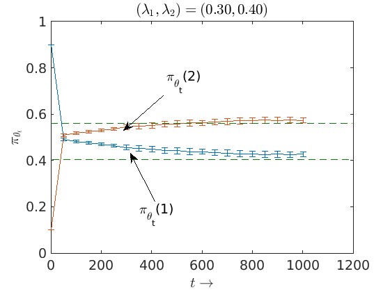
The scheduler is given two base/atomic controllers , i.e. . Controller serves Queue with probability , . As can be seen in Fig. 1(a) when , softmax PG converges to the improper mixture policy that serves each queue independently with probability , which is the delay-optimal controller in . Interestingly, the mixture stabilizes the system whereas both base controllers lead to instability because of insufficient service to some queue. Fig. 1(b) shows that with unequal arrival rates too, Softmax-PG with GradEst quickly converges to the correct improper combination.
Fig. 1(d) shows the evolution of the value function (system backlog) of GradEst (blue) compared with those of the base controllers (red) and the Longest Queue First policy (LQF) which, as the name suggests, always serves the longest queue in the system (black). LQF, like any work-conserving policy, is known to be delay optimal [2].
Finally, Fig. 1(c) shows the result of the second experimental setting with three atomic controllers, one of which is delay optimal. The first two are as before and the third controller, , is LQF. Notice that are both queue length-agnostic, meaning they could attempt to serve empty queues as well. LQF, on the other hand, always and only serves nonempty queues. Hence, in this case the optimal policy is attained at one of the corner points, i.e., . The plot shows the GradEst converging to the correct point on the simplex.
4.2 Time-varying Arrival Rates
We consider a modification to the system in Sec. 6 wherein the arrival rates to the two queues vary over time (adversarially). In particular, varies from . Our PG algorithm successfully tracks this change and adapts to the optimal improper stationary policies in each case as shown in Fig. 2. In all three cases a mixed controller is optimal, and is successfully tracked by our PG algorithm.

5 Conclusion
Our results show that our new improper learning algorithmic framework is able to efficiently learn optimal mixtures of given policies. This paves the way for (a) building more refined theory towards understanding the convergence behavior of such schemes, and (b) benchmarking it more extensively in diverse RL settings including problems of robotic control, computer game playing, etc. This will form the subject of future work.
References
- [1] Flaxman, A. D., Kalai, A. T., and McMahan, H. B. Online convex optimization in the bandit setting: Gradient descent without a gradient. SODA ’05, Society for Industrial and Applied Mathematics, p. 385–394.
- [2] Mohan, A., Chattopadhyay, A., and Kumar, A. Hybrid MAC protocols for low-delay scheduling. In 2016 IEEE 13th International Conference on Mobile Ad Hoc and Sensor Systems (MASS) (Los Alamitos, CA, USA, oct 2016), IEEE Computer Society, pp. 47–55.
- [3] Shakkottai, S., and Stolyar, A. L. Scheduling for multiple flows sharing a time-varying channel: The exponential rule. Translations of the American Mathematical Society-Series 2 207 (2002), 185–202.
- [4] Sutton, R. S., and Barto, A. G. Reinforcement learning: An introduction. MIT press, 2018.
- [5] Tassiulas, L., and Ephremides, A. Stability properties of constrained queueing systems and scheduling policies for maximum throughput in multihop radio networks. IEEE Transactions on Automatic Control 37, 12 (1992), 1936–1948.
- [6] Zaki, M., Mohan, A., Gopalan, A., and Mannor, S. Improper learning with gradient-based policy optimization. arXiv preprint arXiv:2102.08201 (2021).