Deep Spectrum Cartography: Completing Radio Map Tensors Using Learned Neural Models

We are interested in estimating a spatio-spectral radio map of a certain geographical region across a number of frequency bins. The region has $R$ emitters that transmit their signals across certain (possibly overlapping) frequency bands, which together create a power interference field across space and frequency. We consider a rectangular region discretized into $I\times J$ grids and $K$ frequency bins. Hence, the (discretized) power spectral density (PSD) measured over space and frequency gives rise to a 3D radio map that can be expressed as an $I\times J\times K$ tensor $\underline{\bm{X}}\in\mathbb{R}^{I\times J\times K}$, where $\underline{\bm{X}}(i,j,k)$ denotes the PSD of the signal received at location $(i,j)$ and frequency $k$; see Fig. 1 (left). We should mention that although the instantaneous radio map may change quickly, the PSD captures the average spectrum usage over a certain period of time, if the signals are stationary random processes. Hence, estimating PSD-based radio maps is often considered more realistic than estimating the instantaneous situation; see, e.g., [23, 24, 3, 4, 8].

Suppose that there are a number of sensors deployed within this region. We assume that a sensor located at position $(i,j)$ where $i\in[I]$ and $j\in[J]$ can measure the power spectral density (PSD) of its received signal locally over all $K$ frequency bins; i.e., the sensor located at $(i,j)$ can acquire the PSD $\bm{p}_{(i,j)}\in\mathbb{R}^{K}$ of the received signal such that ${\bm{p}}_{(i,j)}=\underline{\bm{X}}(i,j,:)\in\mathbb{R}^{K},$ where $K$ is the number of frequency bins. Note that a vector $\underline{\bm{X}}(i,j,:)$ is also sometimes called a “tensor fiber” [25, 26]. If every location $(i,j)$ has a sensor, a radio map tensor $\underline{\bm{X}}\in\mathbb{R}^{I\times J\times K}$ would be constructed. However, in practice, placing $IJ$ sensors to “cover” the geographical region may not be an viable option. Instead, only a small number of sensors are sparsely placed within the region of interest. In other words, letting

denote the set of sensor locations, we often have $|\bm{\varOmega}|\ll IJ$. Hence, the task of spatio-spectral SC is to estimate the full radio map tensor $\underline{\bm{X}}\in\mathbb{R}^{I\times J\times K}$ using the sensor-acquired measurements (i.e., tensor fibers) $\underline{\bm{X}}(i,j,:)\in\mathbb{R}^{K},\forall(i,j)\in\bm{\varOmega}$—see Fig. 1 (right) for an illustration.

If the spectral band of interest is not large relative to the central carrier frequency (e.g., 20MHz bandwidth at a central carrier frequency within 2-5 GHz.), the spatial propagation pattern of an emitter across different frequencies are identical up to scaling differences caused by the emitter’s PSD. Consequently, if noise is absent, the full radio map can be expressed as follows [16, 8]:

where $\bm{S}_{r}\in\mathbb{R}^{I\times J}$ denotes the spatial loss function (SLF) of the power of emitter $r$, $\bm{c}_{r}\in\mathbb{R}^{K}$ represents the PSD of emitter $r$, $\circ$ is the outer product, and $R$ is the number of emitters in the region of interest. An illustration is shown in Fig. 2. A remark is that the factorization based expression of a radio map also makes storing $\underline{\bm{X}}$ easier. The memory cost of $\underline{\bm{X}}\in\mathbb{R}^{I\times J\times K}$ under (1) is only $O((IJ+K)R)$ other than $O(IJK)$. The memory is even lower when $\bm{S}_{r}$ can be parameterized, e.g., using a low-rank matrix as in [16] or a deep generative model as will be seen in this work.

In essence, the SC problem is an ill-posed inverse problem. Hence, the same insights employed in classic inverse problems, e.g., compressive sensing and low-rank matrix/tensor completion may be used for SC. Indeed, early works exploited the spatial sparsity of emitter locations [6], sparse representation of emitter PSDs in a certain learned domain [13, 4], spatial smoothness of the SLFs [8], and a low-rank tensor structure [16] to come up with radio map recovery formulations. Notably, the most recent work in [16] assumed that ${\rm rank}(\bm{S}_{r})\leq L$ where $L\ll\min\{I,J\}$ and recast the SC problem as a low-rank block-term tensor [27] completion problem. This way, recoverability guarantees of the radio map from sparse sensor measurements can be established.

Structural priors/constraints-assisted inverse problem formulations are useful, but they are often inadequate in dealing with complex scenarios. For example, the low-rank assumption on $\bm{S}_{r}$ is plausible in free space or in rural areas where electromagnetic waveforms could propagate without encountering many barriers. However, the assumption becomes unrealistic when urban or indoor regions are considered. The same challenge is also shared by methods that use spatial smoothness; see, e.g., [8, 28]. Fig. 3 shows how heavy shadowing (caused by barriers like buildings and walls) makes the low-rank and spatial smoothness assumptions on $\bm{S}_{r}$ less accurate. In this example, the first 10 principal components of a $50\times 50$ SLF with little shadowing contain more than 90% energy of the SLF. However, the same number of principal components only contain less than 70% energy of the SLF when the shadowing effect is severe.

Very recently, a couple of data-driven methods were proposed to circumvent the model mismatch challenge. The idea is to learn the complex data generative process (from partial observations) using DNNs through a large number of realistic simulated data samples, and then use the learned neural model to assist radio map completion [18, 17]. For example, the work in [18] generates a training set, denoted by $\{\underline{\bm{X}}_{n}\}_{n=1}^{N}$, where each $\underline{\bm{X}}_{n}\in\mathbb{R}^{I\times J\times K}$ is a radio map tensor following a spatial propagation model [29]. Then, a deep completion network is trained using the following:

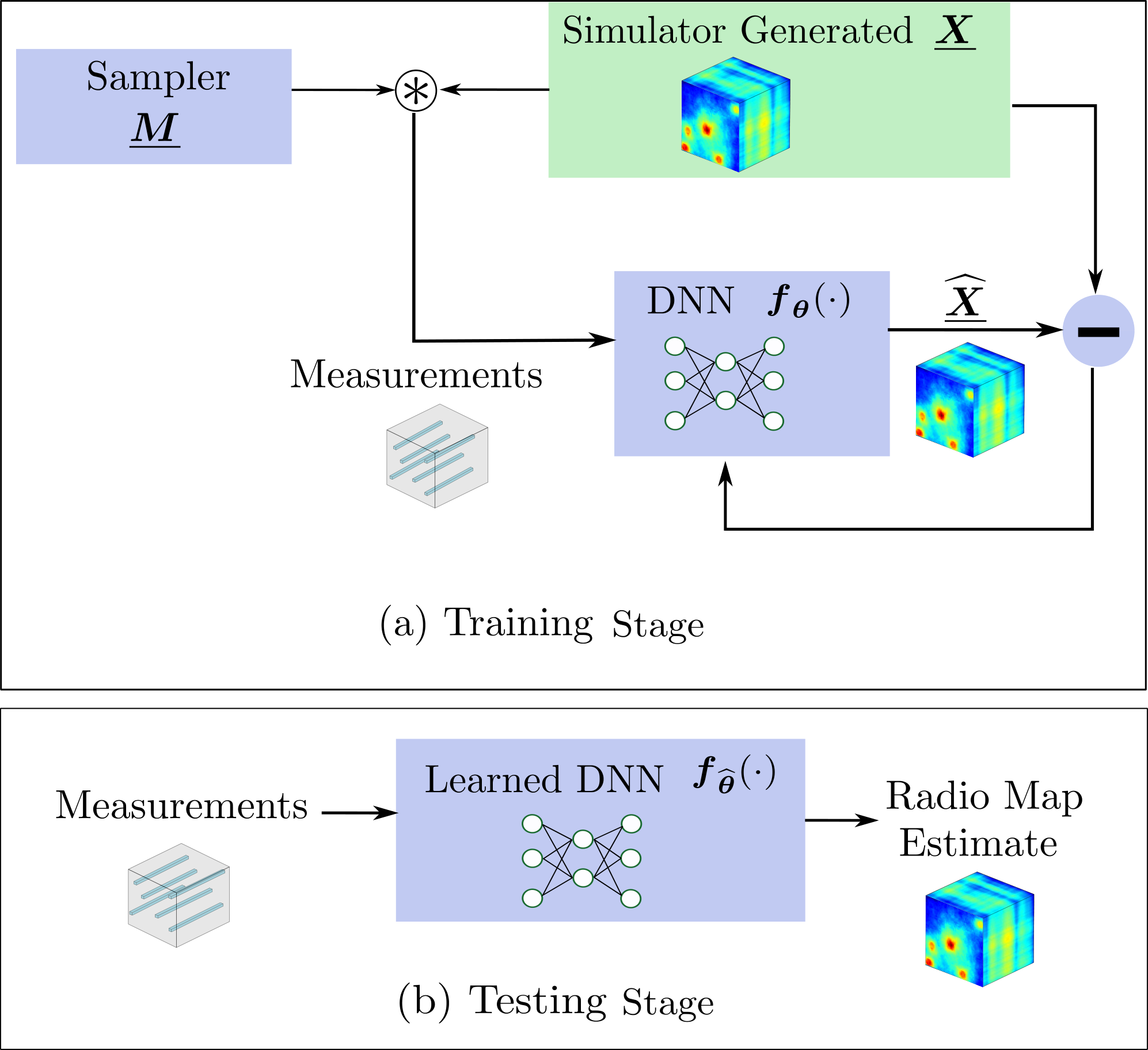
where $\bm{f}_{\bm{\theta}}(\cdot):\mathbb{R}^{I\times J\times K}\rightarrow\mathbb{R}^{I\times J\times K}$ is a DNN whose network weights are collected in $\bm{\theta}$; $\underline{\bm{M}}_{n}\in\mathbb{R}^{I\times J\times K}$ is a mask tensor (or, a sampler) with $\underline{\bm{M}}_{n}(i,j,k)=1$ if the entry in the radio map is sensed, and $\underline{\bm{M}}_{n}(i,j,k)=0$ otherwise¹¹ 1 In practice, the idea in (2) is often carried out with different variations, e.g., slab by slab realization in [18] and [17]. The mask information is also fed to the DNNs together with the sensed data; see details in [18].. After a network $\bm{f}_{\widehat{\bm{\theta}}}$ is learned (via any off-the-shelf DNN training algorithms, e.g., [30]), a radio map can be simply estimated via $\widehat{\underline{\bm{X}}}=\bm{f}_{\widehat{\bm{\theta}}}\left(\underline{\bm{M}}_{\rm sens.}\circledast\underline{\bm{X}}_{\natural}\right)$, where $\underline{\bm{X}}_{\natural}$ is the ground-truth radio map to estimate, $\underline{\bm{M}}_{\rm sens.}$ is the mask tensor that reflects the sensor locations, and $\underline{\bm{M}}_{\rm sens.}\circledast\underline{\bm{X}}_{\natural}$ represents the sensed measurements (i.e., tensor fibers). Specifically, we have $\underline{\bm{M}}_{\rm sens.}(i,j,k)=1,~\forall k,~\text{if}~(i,j)\in\bm{\varOmega}$, and $\underline{\bm{M}}_{\rm sens.}(i,j,k)=0$ otherwise. The major idea of these methods is summarized in Fig. 4.

The most appealing feature of the DL-based SC approaches is that the network $\bm{f}_{\widehat{\bm{\theta}}}$ could potentially complete complex radio maps (e.g., those with heavy shadowing) that handcrafted priors may struggle to model. However, a couple of challenges remain.

Recall that the radio map can be modeled as $\underline{\bm{X}}=\sum_{r=1}^{R}\bm{S}_{r}\circ\bm{c}_{r}$, i.e., aggregated power intensity over space and frequency from $R$ emitters. Due to the difficulty of modeling the $\bm{S}_{r}$’s using handcrafted priors, the performance of model-based methods often degrades in challenging cases, e.g., when heavy shadowing happens. Nonetheless, the model that a radio map is a superposition of individual radio maps associated with the emitters is still accurately reflecting the underlying physics. Hence, instead of learning a DNN to complete the entire aggregated radio map tensor $\underline{\bm{X}}$, our idea is to learn a network for completing the individual $\bm{S}_{r}$’s. If the $\bm{c}_{r}$’s can be somehow estimated, then one can assemble the estimated SLFs and PSDs to recover the entire radio map using (1).

Based on the discussion above, we propose the following process to learn a completion network for individual SLFs:

where $n$ is the training sample index, $\bm{M}_{n}\in\mathbb{R}^{I\times J}$ is the $n$th randomly generated 2D mask, $\bm{Q}_{n}\in\mathbb{R}^{I\times J}$ is a complete SLF of a single emitter, and $\bm{f}_{\bm{\theta}}(\cdot):\mathbb{R}^{I\times J}\rightarrow\mathbb{R}^{I\times J}$ is the SLF completion network to be learned.

After $\bm{f}_{\widehat{\bm{\theta}}}$ is learned, we complete the SLFs by letting

where $\bm{M}_{\rm sens.}$ is the 2D version of sensing mask, in which $\bm{M}_{\rm sens.}(i,j)=1$ if $(i,j)\in\bm{\varOmega}$ and $\bm{M}_{\rm sens.}(i,j)=0$ otherwise. The notation $\bm{M}_{\rm sens.}\circledast{\bm{S}}_{r}$ represents the incomplete individual SLF of emitter $r$—and how to obtain it will be discussed in the next subsection.

In this work, we employ an autoencoder structure for $\bm{f}_{\bm{\theta}}$. Nonetheless, in principle, any generative model such as generative adversarial network (GAN) [32] and variational autoencoder (VAE) [33] can be readily employed into our framework. The autoencoder consists of two major parts, i.e., the encoder and the decoder, respectively. To be more precise, for an ideal anutoencoder that is applied to high-dimensional data $\bm{Q}\in\mathbb{R}^{I\times J}$, we wish the following holds:

in which $\bm{\theta}_{\rm e}$ and $\bm{\theta}_{\bm{d}}$ represents the network parameters of the encoder and decoder, respectively, $\bm{\theta}=[\bm{\theta}_{\rm e}^{\!\top\!},\bm{\theta}_{\rm d}^{\!\top\!}]^{\!\top\!}$, and

denote the encoder and decoder networks, respectively. Notably, if $D\ll IJ$, the model in (5) means that the data matrix $\bm{Q}\in\mathbb{R}^{I\times J}$ can be represented in a low-dimensional latent domain, using its “embedding” $\bm{z}=\bm{p}_{\bm{\theta}_{\rm e}}(\bm{Q})$. The decoder can be regarded as a generator that maps a latent embedding $\bm{z}$ to the observation domain, i.e., to “generate” the ambient data. Hence, the deep autoencoders are also considered as deep generative model learners.

The proposed individual SLF completion method could potentially reduce training costs and improve generalization. However, the inputs to such networks, i.e., $\bm{M}_{\rm sens.}\circledast{\bm{S}}_{r}$ for all $r$, are not observed. Instead, if noise is absent, we observe the following incomplete tensor:

that is acquired by the sensors, where $\underline{\bm{X}}_{\natural}=\sum_{r=1}^{R}\bm{S}_{r}\circ\bm{c}_{r}$ is the target radio map that we aim to recover. If the $\bm{c}_{r}$’s can be somehow estimated, our objective boils down to estimating the incomplete individual SLFs, i.e., $\bm{M}_{\rm sens.}\circledast{\bm{S}}_{r}$ from the observed measurements $\underline{\bm{Y}}$.

To this end, notice that the following relationship holds:

where $\bm{X}_{\natural}={\rm unfold}(\underline{\bm{X}}_{\natural})\in\mathbb{R}^{K\times IJ}$ and the tensor unfolding operator is defined as $\bm{X}_{\natural}(:,q)=\underline{\bm{X}}_{\natural}(i,j,:),\quad q=I(i-1)+j$.

Clearly, if we define $\bm{G}:=\bm{Y}(:,\bm{\varOmega}_{\rm col})$, where $\bm{\varOmega}_{\rm col}\subseteq[IJ]$ such that $q=I(i-1)+j\in\bm{\varOmega}_{\rm col},\quad\forall(i,j)\in\bm{\varOmega}$, then, we have the following expression for $\bm{G}$:

where $\bm{C}=[\bm{c}_{1},\ldots,\bm{c}_{R}]\in\mathbb{R}^{K\times R}$ and $\bm{S}=[{\rm vec}(\bm{S}_{1}),\ldots,{\rm vec}(\bm{S}_{R})]^{\!\top\!}\in\mathbb{R}^{R\times IJ}$.

If one could estimate $\bm{H}$, then define a matrix ${\bm{S}}_{\rm miss}\in\mathbb{R}^{R\times IJ}$ such that ${\bm{S}}_{\rm miss}(r,\bm{\varOmega}_{\rm col}):=\bm{H}(r,:)$. Further, let ${\bm{S}}_{\rm miss}(:,\bm{\varOmega}_{\rm col}^{\rm c})=\bm{0}$, where $\bm{\varOmega}_{\rm col}^{\rm c}$ is the complement of $\bm{\varOmega}_{\rm col}$. As a consequence, we have

where the matricization operator ${\rm mat}(\cdot):\mathbb{R}^{IJ}\rightarrow\mathbb{R}^{I\times J}$ is the inverse operation of vectorization. Note that $\bm{P}_{r}$ is the incomplete individual radio map that we wish to feed to $\bm{f}_{\widehat{\bm{\theta}}}(\cdot)$ in (4). The procedure for creating the matrix $\bm{G}$ is illustrated in Fig. 6 (a).

Note that $\bm{C}$ and $\bm{H}$ are are both nonnegative matrices, per their physical meanings. Hence, our task amounts to estimating $\bm{C}$ and $\bm{H}$ from $\bm{G}$—which is an NMF problem [34]. Then, we take the estimated $\bm{H}$’s rows and apply deep network-based completion to estimate $\bm{S}_{r}$ for all $r$. With $\bm{C}$ and $\bm{S}_{r}$’s estimated, we can recover $\underline{\bm{X}}_{\natural}$; see the overall procedure in Fig. 6.

Note that NMF is not always unique—i.e., estimating $\bm{C}$ and $\bm{H}$ from $\bm{G}$ may not be always possible; see discussions about NMF identifiability in the literature, e.g., [35, 34, 36]. Nonetheless, if the emitters transmit sparsely across the spectral band, estimating $\bm{C}$ and $\bm{H}$ via NMF is viable. To see this, we make the following assumption:

Assumption 1 is considered reasonable since emitters often take different carrier frequencies (or subbands in OFDM systems) [24]. In addition, if the emitters use the $K$ frequencies in a sparse manner, such an assumption is often not hard to meet. Under Assumption 1, we show that:

The proof is relegated to Appendix B. Note that Assumption 1 translates to the separability condition in the context of NMF, and the proof of Theorem 1 is a direct application of identifiability of separable NMF [34, 36]. Note that under separability condition, NMF is solvable using either greedy algorithms [19, 20] or convex optimization [37], both of which are polynomial-time algorithms. In this work, we employ the Gram-Schmidt-like successive projection algorithm (SPA) algorithm in [19, 20] due to its efficiency; see [34, 19, 20] and Appendix G for details of the SPA algorithm.

With the learned $\bm{f}_{\widehat{\bm{\theta}}}$ and the estimated $\widehat{\bm{P}}_{r}$ [cf. Eq. (10)] from the NMF stage, we complete the SLFs by letting $\widehat{\bm{S}}_{r}\leftarrow\bm{f}_{\widehat{\bm{\theta}}}\left(\widehat{\bm{P}}_{r}\right)$. The two-stage process is summarized in Algorithm 1, which we will refer to as the nonnegative matrix factorization assisted deep emitter spatial loss completion (Nasdac). One remark is that although all NMF algorithms admit inevitable scaling and permutation ambiguities (i.e., the $\bm{\varLambda}$ and $\bm{\varPi}$ matrices in Theorem 1 cannot be removed), these ambiguities do not affect the reconstruction, if $\widehat{\bm{C}}=\bm{C}\bm{\varPi}\bm{\varLambda},~\widehat{\bm{H}}=\bm{\varLambda}^{-1}\bm{\varPi}^{\!\top\!}\bm{H}$ hold—since the ambiguity matrices cancel each other in the final assembling stage (i.e., line 1 in Algorithm 1).

Note that in Nasdac, the number of emitters $R$ is assumed to be previously estimated or known. Under the considered scenario, estimating $R$ corresponds to estimating the rank of the NMF model $\bm{G}\approx\bm{C}\bm{H}$ [cf. Eq. (29)]. This can be accomplished by existing model-order selection methods (see [38] for an overview). Many methods for rank estimation under noisy NMF models can also be used, e.g., [20, 39, 40, 41].

In this subsection, we analyze the recoverability of the ground-truth radio map tensor $\underline{\bm{X}}_{\natural}$ under the criterion in (12). In our analysis, we treat $\underline{\bm{X}}_{\natural}$ as a deterministic term, while the set of sampling locations specified by $\bm{\varOmega}$ are random. To proceed, first, consider the following assumption on the employed neural network in our framework:

Note that many neural network structures (e.g., the fully connected network (FCN) and the convolutional neural network (CNN)) satisfy the structure specified in Assumption 2. Popular activation functions such as Sigmoid and ReLU are also Lipstchitz continuous. We will use the following definitions:

In principle, any norm can be used to define an $\varepsilon$-net. We use the Euclidean norm in this work. The covering number is a way of measuring the “complexity” of a continuous set using its discretized version.

Note that $\widehat{\sf Loss}$ can be understood as the “empirical loss” measured at a solution $\widetilde{\underline{\bm{X}}}\in{\cal X}_{R,\bm{g}_{\bm{\theta}_{d}}}$, and ${\sf Loss}$ is the “true” loss measured over the complete data (or, the generalization error). Under the above definitions, we first show the following Lemma:

We also show the following:

Using the above lemmas and definitions, we present our main recoverability theorem:

Theorem 2 asserts that the criterion in (12) admits recoverability of the ground-truth radio map $\underline{\bm{X}}_{\natural}$—even if there exists sensing noise and the learned generative model is not perfect. The recovery error consists of three main sources, namely, the sensing noise $\underline{\bm{N}}$, sampling-induced noise (or, generalization error) ${\sf Gap}^{\star}({\bm{\varOmega}})$ and the generative model’s representation error, i.e., ${\sf Err}_{\rm rep}({{\cal X}_{R,\bm{g}_{\bm{\theta}_{\rm d}}}})$. If a more complex (i.e., deeper and/or wider) neural network is used—which means that the generative model can approximate more complex SLFs—then the representation error can be reduced. However, using a more complex neural network will make the covering number of the solution set increase, and thus ${\sf Gap}^{\star}({\bm{\varOmega}})$ increases—which presents a trade-off between network expressiveness and recovery accuracy. In addition, when $|\bm{\varOmega}|$ approaches $IJ$ and $I,J$ grow large, the sampling-induced error ${\sf Gap}^{\star}({\bm{\varOmega}})$ approaches zero [cf. Eq. (13)].

A remark is that although the theorem statement assumes a known $R$, it can also be used to understand the cases where $R$ is not exactly known (or wrongly estimated). When $\widehat{R}=R^{\prime}$ is underestimated, the energy of the missed components $\bm{S}_{r}\circ\bm{c}_{r}$ for $R^{\prime}<r\leq R$ can be absorbed into the noise term $\underline{\bm{N}}$. When $\widehat{R}$ is overestimated, $\underline{\bm{X}}_{\natural}$ can still be expressed by using (1), with some redundant/spurious components. The redundant components do not create any new noise terms, but will increase the covering number of the model. This means that more samples will be required for attaining the same bound of recoverability accuracy—which is the price to pay for overestimating $R$.

We propose an alternating optimization algorithm to handle the formulated problem in (12); i.e., we tackle subproblems w.r.t. $\bm{C}$ and $\bm{Z}=[\bm{z}_{1},\ldots,\bm{z}_{R}]$ alternately, until a certain convergence criterion is met.

Note that the $\bm{C}$-subproblem can be re-expressed as follows:

where $\bm{G}$ is defined as before, $\bm{H}^{(k)}(r,:)=\bm{S}^{(k)}(r,\bm{\Omega}_{\rm col})$, and $\bm{S}^{(k)}(r,:)={\rm vec}(\bm{g}_{\bm{\theta}_{\rm d}}(\bm{z}_{r}))^{\!\top\!}$ is the (vectorized) current estimate for the $r$th SLF at iteration $k$. The problem in (15) is a nonnegativity-constrained least squares (NNLS) problem—which admits a plethora of off-the-shelf solvers. In this work, we employ the NNLS algorithm proposed in [44] that strikes a good balance between speed and accuracy.

As for the $\bm{z}_{r}$-subproblem, since it involves deep neural networks, any back-propagation-based gradient descent-related algorithms can be used [42]. To be specific, we use the update $\bm{Z}^{(k_{t+1})}\leftarrow\bm{Z}^{(k_{t})}-\gamma^{t}\overline{\nabla}_{\bm{Z}}f(\bm{Z}^{(k_{t})};\bm{C}^{(k+1)})$, and we let $\bm{Z}^{(k_{0})}\leftarrow\bm{Z}^{(k)}$, $\bm{Z}^{(k+1)}\leftarrow\bm{Z}^{(k_{T})}$, where $T$ is the number of gradient iterations (inner iterations) used for handling the $\bm{Z}$-subproblem in the $k$th outer iteration (that alternates between $\bm{Z}$ and $\bm{C}$), $\gamma^{t}$ is the step size in the $t$th inner iteration, and $\bm{Z}=[\bm{z}_{1},\ldots,\bm{z}_{R}]$. We have used the notation

and $\overline{\nabla}_{\bm{Z}}f$ is a gradient-based direction, e.g., momentum-based gradient or scaled gradient (such as those used in Adagrad [45] and Adam [30]), which can often be constructed from the gradient ${\nabla}_{\bm{Z}}f$. The gradient of $f$ w.r.t. $\bm{Z}$ can be computed via the chain rule and back-propagation. In this work, we employ the popularized gradient evaluation tool, namely, autograd in Pytorch [45], to carry out the computation. The step size $\gamma^{t}$ and $\overline{\nabla}_{\bm{Z}}f$ follow the Adam strategy [30], and $\gamma^{t}$ has an initial value of $0.01$. The algorithm is summarized in Algorithm 2, which is referred to as the Deep generative PriOr With Joint OptimizatioN for Spectrum cartography (DowJons) algorithm.

The DowJons algorithm is an alternating optimization (AO) algorithm where the $\bm{Z}$ block is nonconex. This means that one often does not optimally solve the $\bm{Z}$-subproblem in practice. Nonetheless, we observe that DowJons converges well even if the $\bm{Z}$-subproblem is executed with only a few iterations. Indeed, under some conditions, one can show that such an “inexact” AO procedure produces a solution sequence that converges to the vicinity of a stationary point of (12). Discussions on DowJons’s convergence properties can be found in Appendix C.

References

- [1] F. C. Commission, “FCC notice of proposed rulemaking FCC 04-113,” 2004.
- [2] Z. Tian and G. B. Giannakis, “Compressed sensing for wideband cognitive radios,” in Proc. IEEE ICASSP, 2007, pp. IV–1357.
- [3] X. Fu, N. D. Sidiropoulos, J. H. Tranter, and W.-K. Ma, “A factor analysis framework for power spectra separation and multiple emitter localization,” IEEE Trans. Signal Process., vol. 63, no. 24, pp. 6581–6594, 2015.
- [4] J. A. Bazerque and G. B. Giannakis, “Distributed spectrum sensing for cognitive radio networks by exploiting sparsity,” IEEE Trans. Signal Process., vol. 58, no. 3, pp. 1847–1862, 2010.
- [5] Y. Arjoune and N. Kaabouch, “A comprehensive survey on spectrum sensing in cognitive radio networks: Recent advances, new challenges, and future research directions,” Sensors, vol. 19, no. 1, p. 126, 2019.
- [6] B. A. Jayawickrama, E. Dutkiewicz, I. Oppermann, G. Fang, and J. Ding, “Improved performance of spectrum cartography based on compressive sensing in cognitive radio networks,” in Proc. ICC, 2013, pp. 5657–5661.
- [7] G. Boccolini, G. Hernandez-Penaloza, and B. Beferull-Lozano, “Wireless sensor network for spectrum cartography based on kriging interpolation,” in Proc. IEEE Int. Symp. PIMRC, 2012, pp. 1565–1570.
- [8] J. A. Bazerque, G. Mateos, and G. B. Giannakis, “Group-lasso on splines for spectrum cartography,” IEEE Trans. Signal Process., vol. 59, no. 10, pp. 4648–4663, 2011.
- [9] S. Bi, J. Lyu, Z. Ding, and R. Zhang, “Engineering radio maps for wireless resource management,” IEEE Trans. Wireless Commun., vol. 26, no. 2, pp. 133–141, 2019.
- [10] C. I. Kanatsoulis, X. Fu, N. D. Sidiropoulos, and M. Akçakaya, “Tensor completion from regular sub-Nyquist samples,” IEEE Trans. Signal Process., vol. 68, pp. 1–16, 2019.
- [11] M. Yuan and C.-H. Zhang, “On tensor completion via nuclear norm minimization,” Foundations of Computational Mathematics, vol. 16, no. 4, pp. 1031–1068, 2016.
- [12] B. A. Jayawickrama, E. Dutkiewicz, I. Oppermann, and M. Mueck, “Iteratively reweighted compressive sensing based algorithm for spectrum cartography in cognitive radio networks,” in Proc. IEEE WCNC, 2014, pp. 719–724.
- [13] S.-J. Kim and G. B. Giannakis, “Cognitive radio spectrum prediction using dictionary learning,” in Proc. IEEE GLOBECOM, 2013, pp. 3206–3211.
- [14] M. Hamid and B. Beferull-Lozano, “Non-parametric spectrum cartography using adaptive radial basis functions,” in Proc. IEEE ICASSP, 2017, pp. 3599–3603.
- [15] D. Romero, S.-J. Kim, G. B. Giannakis, and R. López-Valcarce, “Learning power spectrum maps from quantized power measurements,” IEEE Trans. Signal Process., vol. 65, no. 10, pp. 2547–2560, 2017.
- [16] G. Zhang, X. Fu, J. Wang, X.-L. Zhao, and M. Hong, “Spectrum cartography via coupled block-term tensor decomposition,” IEEE Trans. SIgnal Process., vol. 68, pp. 3660–3675, 2020.
- [17] X. Han, L. Xue, F. Shao, and Y. Xu, “A power spectrum maps estimation algorithm based on generative adversarial networks for underlay cognitive radio networks,” Sensors, vol. 20, no. 1, p. 311, 2020.
- [18] Y. Teganya and D. Romero, “Data-driven spectrum cartography via deep completion autoencoders,” in Proc. IEEE ICC, 2020, pp. 1–7.
- [19] N. Gillis and S. A. Vavasis, “Fast and robust recursive algorithms for separable nonnegative matrix factorization,” IEEE Trans. Pattern Anal. Mach. Intell., vol. 36, no. 4, pp. 698–714, 2013.
- [20] X. Fu, W.-K. Ma, T.-H. Chan, and J. M. Bioucas-Dias, “Self-dictionary sparse regression for hyperspectral unmixing: Greedy pursuit and pure pixel search are related,” IEEE J. Sel. Topics Signal Process., vol. 9, no. 6, pp. 1128–1141, 2015.
- [21] T. King, S. Kopf, T. Haenselmann, C. Lubberger, and W. Effelsberg, “CRAWDAD dataset mannheim/compass (v. 2008-04-11),” Downloaded from https://crawdad.org/mannheim/compass/20080411, Apr. 2008.
- [22] S. Shrestha, X. Fu, and M. Hong, “Deep generative model learning for blind spectrum cartogrphy with nmf-based radio map dissaggregation,” in Proc. IEEE ICASSP, to appear, 2021.
- [23] O. Mehanna and N. D. Sidiropoulos, “Frugal sensing: Wideband power spectrum sensing from few bits,” IEEE Trans. Signal Process., vol. 61, no. 10, pp. 2693–2703, 2013.
- [24] X. Fu, N. D. Sidiropoulos, and W.-K. Ma, “Power spectra separation via structured matrix factorization.” IEEE Trans. Signal Process., vol. 64, no. 17, pp. 4592–4605, 2016.
- [25] X. Fu, S. Ibrahim, H.-T. Wai, C. Gao, and K. Huang, “Block-randomized stochastic proximal gradient for low-rank tensor factorization,” IEEE Trans. Signal Process., vol. 68, pp. 2170–2185, 2020.
- [26] X. Fu, N. Vervliet, L. De Lathauwer, K. Huang, and N. Gillis, “Computing large-scale matrix and tensor decomposition with structured factors: A unified nonconvex optimization perspective,” IEEE Signal Process. Mag., vol. 37, no. 5, pp. 78–94, 2020.
- [27] L. De Lathauwer, “Decompositions of a higher-order tensor in block terms—Part II: Definitions and uniqueness,” SIAM J. Matrix Anal. Appl., vol. 30, no. 3, pp. 1033–1066, 2008.
- [28] T. Yucek and H. Arslan, “A survey of spectrum sensing algorithms for cognitive radio applications,” IEEE Commun. Surveys Tuts., vol. 11, no. 1, pp. 116–130, 2009.
- [29] A. Goldsmith, Wireless communications. Cambridge university press, 2005.
- [30] D. P. Kingma and J. Ba, “Adam: A method for stochastic optimization,” in Proc. ICLR, 2015.
- [31] P. Stoica, R. L. Moses et al., Spectral analysis of signals. Pearson Prentice Hall Upper Saddle River, NJ, 2005.
- [32] I. J. Goodfellow, J. Pouget-Abadie, M. Mirza, B. Xu, D. Warde-Farley, S. Ozair, A. C. Courville, and Y. Bengio, “Generative adversarial nets,” in Proc. NeurIPS, 2014.
- [33] D. P. Kingma and M. Welling, “Auto-encoding variational bayes,” in Proc. ICLR, 2013.
- [34] X. Fu, K. Huang, N. D. Sidiropoulos, and W.-K. Ma, “Nonnegative matrix factorization for signal and data analytics: Identifiability, algorithms, and applications.” IEEE Signal Process. Mag., vol. 36, no. 2, pp. 59–80, 2019.
- [35] X. Fu, K. Huang, and N. D. Sidiropoulos, “On identifiability of nonnegative matrix factorization,” IEEE Signal Process. Lett., vol. 25, no. 3, pp. 328–332, 2018.
- [36] N. Gillis, Nonnegative Matrix Factorization. SIAM, 2020.
- [37] N. Gillis and R. Luce, “Robust near-separable nonnegative matrix factorization using linear optimization,” The Journal of Machine Learning Research, vol. 15, no. 1, pp. 1249–1280, 2014.
- [38] P. Stoica and Y. Selen, “Model-order selection: a review of information criterion rules,” IEEE Signal Processing Magazine, vol. 21, no. 4, pp. 36–47, 2004.
- [39] X. Fu and W.-K. Ma, “Robustness analysis of structured matrix factorization via self-dictionary mixed-norm optimization,” IEEE Signal Process. Lett., vol. 23, no. 1, pp. 60–64, 2016.
- [40] J. M. Bioucas-Dias and J. M. P. Nascimento, “Hyperspectral subspace identification,” IEEE Trans. Geosci. Remote Sensi., vol. 46, no. 8, pp. 2435–2445, 2008.
- [41] A. Ambikapathi, T.-H. Chan, C.-Y. Chi, and K. Keizer, “Hyperspectral data geometry-based estimation of number of endmembers using p-norm-based pure pixel identification algorithm,” IEEE Trans. Geosci. Remote Sens., vol. 51, no. 5, pp. 2753–2769, 2012.
- [42] I. Goodfellow, Y. Bengio, A. Courville, and Y. Bengio, Deep learning. MIT press Cambridge, 2016, vol. 1, no. 2.
- [43] D.-X. Zhou, “The covering number in learning theory,” Journal of Complexity, vol. 18, no. 3, pp. 739–767, 2002.
- [44] C. L. Lawson and R. J. Hanson, Solving least squares problems. SIAM, 1995.
- [45] Pytorch, “torch.autograd.” [Online]. Available: https://pytorch.org/docs/stable/autograd.html
- [46] S. Üreten, A. Yongaçoğlu, and E. Petriu, “A comparison of interference cartography generation techniques in cognitive radio networks,” in Proc. IEEE ICC, 2012, pp. 1879–1883.
- [47] M. N. Hindia, A. M. Al-Samman, T. A. Rahman, and T. Yazdani, “Outdoor large-scale path loss characterization in an urban environment at 26, 28, 36, and 38 ghz,” Physical Communication, vol. 27, pp. 150–160, 2018.
- [48] C. Battaglino, G. Ballard, and T. G. Kolda, “A practical randomized cp tensor decomposition,” SIAM Journal on Matrix Analysis and Applications, vol. 39, no. 2, pp. 876–901, 2018.
- [49] D. Pollard, “Empirical processes: theory and applications,” in NSF-CBMS regional conference series in probability and statistics. JSTOR, 1990, pp. i–86.
- [50] Y.-X. Wang and H. Xu, “Stability of matrix factorization for collaborative filtering,” arXiv preprint arXiv:1206.4640, 2012.
- [51] R. J. Serfling, “Probability inequalities for the sum in sampling without replacement,” The Annals of Statistics, pp. 39–48, 1974.
- [52] X. Fu, W.-K. Ma, K. Huang, and N. D. Sidiropoulos, “Blind separation of quasi-stationary sources: Exploiting convex geometry in covariance domain,” IEEE Transa. Signal Process., vol. 63, no. 9, pp. 2306–2320, 2015.
- [53] D. L. Donoho et al., “Compressed sensing,” IEEE Trans. Inf. Theory, vol. 52, no. 4, pp. 1289–1306, 2006.
![[Uncaptioned image]](2105.00177v2/authors/sagar.jpg) |
Sagar Shrestha received his B.Eng. in Electronics and Communication Engineering from Pulchowk Campus of Tribhuvan University, Kathmandu, Nepal, in 2016. He is currently working towards a Ph.D. degree at the School of Electrical Engineering and Computer Science, Oregon State University, Corvallis, OR, USA. His current research interests are in the broad area of statistical machine learning and signal processing. |
![[Uncaptioned image]](2105.00177v2/authors/xiaofu.jpg) |
Xiao Fu (Senior Member, IEEE) received the B.Eng. and MSc. degrees from the University of Electronic Science and Technology of China (UESTC), Chengdu, China, in 2005 and 2010, respectively. He received the Ph.D. degree in Electronic Engineering from The Chinese University of Hong Kong (CUHK), Shatin, N.T., Hong Kong, in 2014. He was a Postdoctoral Associate with the Department of Electrical and Computer Engineering, University of Minnesota, Minneapolis, MN, USA, from 2014 to 2017. Since 2017, he has been an Assistant Professor with the School of Electrical Engineering and Computer Science, Oregon State University, Corvallis, OR, USA. His research interests include the broad area of signal processing and machine learning. Dr. Fu received a Best Student Paper Award at ICASSP 2014, and was a recipient of the Outstanding Postdoctoral Scholar Award at University of Minnesota in 2016. His coauthored papers that received Best Student Paper Awards from IEEE CAMSAP 2015 and IEEE MLSP 2019, respectively. He serves as a member of the Sensor Array and Multichannel Technical Committee (SAM-TC) of the IEEE Signal Processing Society (SPS). He is also a member of the Signal Processing for Multisensor Systems Technical Area Committee (SPMuS-TAC) of EURASIP. He is the Treasurer of the IEEE SPS Oregon Chapter. He serves as an Editor of Signal Processing. He was a tutorial speaker at ICASSP 2017 and SIAM Conference on Applied Linear Algebra 2021. |
![[Uncaptioned image]](2105.00177v2/authors/mingyihong.jpg) |
Mingyi Hong (Senior Member, IEEE) received the Ph.D. degree from the University of Virginia, Charlottesville, in 2011. He is an Associate Professor with the Department of Electrical and Computer Engineering, the University of Minnesota, Minneapolis. He is on the IEEE Signal Processing for Communications and Networking Technical Committee, and he is an Associate Editor for IEEE TRANSACTIONS ON SIGNAL PROCESSING. His research interests include optimization theory and applications in signal processing and machine learning. |
Supplementary Material of “Deep Spectrum Cartography: Completing Radio Map Tensors Using Learned Neural Models”
S. Shrestha, X. Fu, and M. Hong
Appendix C Convergence Properties of DowJons
We briefly discuss some convergence properties of DowJons in this appendix. For simplicity, we consider , i.e., the plain vanilla gradient descent approach is used for updating . Our proof can be generalized to cover cases where stochastic gradient is used, e.g., by combining with proof ideas from fiber sampling-based stochastic tensor decomposition [25, 26, 48]. Under this setting, we have the following result:
Proposition 1.
Assume that the learned generative model satisfies for all possible , that is full rank for all , and is uniformly upper bounded by for all . Also assume that at a given iteration , the following holds: