High-energy cosmic neutrinos as a probe of the vector mediator scenario in light of the muon anomaly and Hubble tension
Abstract
We show that Gen-2 can probe
Abstract
In light of the recent Muon experiment data from Fermilab, we investigate the implications of a gauged model for high energy neutrino telescopes. It has been suggested that a new gauge boson at the MeV scale can both account for the Muon data and alleviate the tension in the Hubble parameter measurements. It also strikes signals at IceCube from the predicted resonance scattering between high-energy neutrinos and the cosmic neutrino background. We revisit this model based on the latest IceCube shower data, and perform a four-parameter fit to find a preferred region. We do not find evidence for secret interactions. The best-fit points of and are MeV and , respectively, depending on assumptions regarding the absolute neutrino masses, and the secret interaction parameter space allowed by the observed IceCube data overlaps with the regions of the parameter space that can explain the muon anomaly and Hubble tension as well. We demonstrate that future neutrino telescopes such as IceCube-Gen2 can probe this unique parameter space, and point out that successful measurements would infer the neutrino mass with .
I Introduction
The recent data from the Fermilab Muon Collaboration indicates that muon magnetic moment may disagree with phenomenological predictions from the Standard Model (SM) Abi et al. 2021 consistent with the earlier E821 experiment at Brookhaven Bennett et al. 2006. Although it could be explained by the SM physics through the hadronic vacuum polarization (Davier et al. 2011; Davier et al. 2017; Davier et al. 2020; Borsanyi et al. 2021), this may indicate beyond the Standard Model (BSM) physics coupled to the muons. As a consequence of electroweak gauge symmetry, modifications to muon physics would imply modified neutrino physics as well given that charged leptons and neutrinos come together in doublets. In this paper, we explore an example of this in the context of gauged lepton number. A very large number of possible interpretations of the new Muon g-2 results have already appeared, including supersymmetry Zhang et al. 2022; Baum et al. 2022; Ahmed et al. 2022; Cox et al. 2021; Abdughani et al. 2021; Van Beekveld et al. 2021; Yin 2021; Han 2021; Buen-Abad et al. 2021; Wang et al. 2021a; Cao et al. 2021; Gu et al. 2021; Athron et al. 2021; Aboubrahim et al. 2021; Yang et al. 2021 new gauge symmetries Greljo et al. 2021; Zu et al. 2022; Cadeddu et al. 2021; Yang et al. 2021; Kawamura and Raby 2021; Li et al. 2021a; Borah et al. 2021; Buras et al. 2021, dark matter Arcadi et al. 2021; Bai and Berger 2021; Zu et al. 2022; Lu et al. 2021 axions and axion-like particles Ge et al. 2021; Brdar et al. 2021, Higgs doublet models Ferreira et al. 2021; Wang et al. 2021b; Chen et al. 2021; Athron et al. 2021; Chun and Mondal 2021; Arcadi et al. 2022; Li et al. 2021a, 331 models Li et al. 2021b, seesaw models Escribano et al. 2021 and leptoquarks Coluccio Leskow et al. 2017; Crivellin et al. 2021
As is well known, gauging the lepton number combination is anomaly free He et al. 1991a; He et al. 1991b. It is also experimentally challenging to probe given that its main effects are to modify the interactions of unstable charged leptons and neutrinos. Intriguingly, this combination of gauged lepton numbers can both explain and be consistent with the constraints from null experiments Altmannshofer et al. 2014a; Altmannshofer et al. 2014b; Bauer et al. 2018. In principle, this scenario can be tested at NA64, the European Spallation Source, DARWIN Amaral et al. 2021, the Missing Muon Momentum () experiment at Fermilab Kahn et al. 2018, and the High Luminosity-LHC Galon et al. 2020.
This work focuses on a different probe of gauged , involving only neutrinos. We study the current and future sensitivity of the IceCube neutrino telescope to such new gauge interactions, by examining in detailed the modifications to the spectrum of high-energy cosmic events Ioka and Murase 2014; Ng and Beacom 2014. Such interactions can also alleviate the tension in Hubble parameters between the local value and cosmic microwave background (CMB) data, through delaying the neutrino free-streaming by self-interactions Cyr-Racine and Sigurdson 2014; Archidiacono and Hannestad 2014; Lancaster et al. 2017; Oldengott et al. 2017; Kreisch et al. 2020; Blinov et al. 2019 or adding to the effective number of relativistic (neutrino) species Weinberg 2013; Berlin and Blinov 2019; D’Eramo et al. 2018; Escudero et al. 2019. We find that the data from IceCube and the Muon collaboration can be combined to yield a non-trivial determination of neutrino masses. Earlier work has also examined the impact of gauged at IceCube Araki et al. 2015; Kamada and Yu 2015; DiFranzo and Hooper 2015. We also note that extended gauge symmetries (e.g., different baryon and lepton number combinations) may allow one to also connect to the LMA-Dark solution of neutrino oscillations for gauge boson masses in the range we are considering here Farzan 2015; Denton et al. 2018. We note that Ref. Okada and Seto 2020 commented on the connections between IceCube, Hubble tension, and muon in the model.
In Fig. 1 we show the IceCube preferred region in red in the plane of the gauge boson mass and the neutrino mass. Here the resonance energy in the observer frame is , where is the typical redshift of the neutrino sources. The gray shaded area shows the region of neutrino masses excluded by cosmology. Given that none of the individual neutrino masses can exceed the cosmological bound on the sum of neutrino masses, we display the Planck 2018 bound Aghanim et al. 2020. Notice that the region between MeV shows the range of the gauge boson mass that may explain the observations while remaining consistent with the null results from CCFR Altmannshofer et al. 2014b; Mishra et al. 1991 and Borexino Kamada and Yu 2015; Harnik et al. 2012; Bellini et al. 2011. For simplicity we have assumed the natural level of loop-induced kinetic mixing for the Borexino constraint, but in principle this can be relaxed by allowing model-dependent additional particles in the loop. This would only allow for slightly lighter gauge boson masses. Similar masses and gauge couplings can also alleviate the Hubble tension via the extra contribution to the radiation density from the light vector particle (e.g., Ref. Escudero et al. 2019).
The remainder of this paper is as follows. In the next section, we introduce the model and the neutrino-neutrino cross section the model predicts. In Sec. III we consider implications of the present IceCube shower data can provide, being careful to allow for fairly weak priors on both particle and astrophysical parameters. We discuss the potential of the next generation detectors in confirming or excluding the model in Sec. IV and we conclude in Sec. V.
II Gauged Model
We consider a model of the gauged number He et al. 1991a; He et al. 1991b, with the Lagrangian
| (1) |
where is the gauge coupling, is the new gauge boson with mass , and the current associated with the new symmetry is
| (2) |
where is the lepton doublet of the generation. This new gauge interaction allows for high-energy neutrinos to scatter on the neutrinos of the cosmic neutrino background (CB). The most significant effect is the -channel scattering cross section, which in terms of mass eigenstates can be written as,
| (3) |
where for a given incoming neutrino energy the Mandelstam variable is , where are the masses of the mostly active neutrinos, and the width is . We have also defined the effective charge in the above for scattering of the mass eigenstates: , where , and is the Pontecorvo–Maki–Nakagawa–Sakata (PMNS) matrix. In principle, the -channel contributions can also be relevant at large couplings, e.g. Blum et al. 2014; Cherry et al. 2014; Cherry et al. 2016, which is out of the range we consider in this work, and we have checked numerically that we can neglect it here.
The neutrinos scattering off each other can cause the depletion of astrophysical neutrinos at the resonant energies Ioka and Murase 2014; Ng and Beacom 2014; Ibe and Kaneta 2014. Because of , the cross section would be localized around : where is the effective cross section, averaged over the resonance width. We can calculate the neutrino optical depth as Creque-Sarbinowski et al. 2021:
| (4) |
using , where , and is the neutrino number density. Here is the Hubble parameter at redshift and is the Heaviside function. We can calculate the flux of BSM-mediated astrophysical neutrinos as (e.g., Murase et al. 2016)
| (5) |
where is the differential rate density of the astrophysical neutrinos. For the redshift evolution of sources, , we assume that they are distributed according to the star-formation rate Yuksel et al. 2008. We do not consider effects of cascades as an approximation, which is reasonable because its effect is a factor of 2 for we consider Blum et al. 2014.
Finally, because the neutrino decoherence time scale is much smaller than other relevant time scales, the fluxes of the neutrino flavors are given by .
III Implications of High-Energy Neutrino Data
Secret neutrino self-interactions lead to striking spectral distortions at IceCube Ioka and Murase 2014; Ng and Beacom 2014; Ibe and Kaneta 2014; Blum et al. 2014; Araki et al. 2015. To find this spectral feature, it is crucial to use a data sample with a good energy resolution. High-energy starting events (HESEs), including showers and starting tracks, are often used, in which the deposit energy distribution is calculated Blum et al. 2014; Shoemaker and Murase 2016. For this purpose, for our numerical analysis we use the 6-yr shower data sample of IceCube, which is dominated by the electron and tau contributions to the data Aartsen et al. 2020a. This has an advantage of having more events especially at lower energies, which enables us to determine the spectral index (defined below) better. (Note that the 6-yr shower analysis result, , is consistent with the 7.5 yr HESE analysis result, Abbasi et al. 2020, within ). The ordinary SM fit that the IceCube collaboration performs, fits to an unbroken power-law with the slope
| (6) | |||||
where
is the all-flavor flux at 100 TeV. The IceCube collaboration officially found the best-fit values, and .
To perform our analysis, instead of calculating the expected number of events we calculate at each bin of energy and compare it with the flux data given in Fig. 3 of Ref. Aartsen et al. 2020a. We define the following log-likelihood function:
| (7) | |||||
where are the IceCube cascade fluxes at each bin of energy while is the theory prediction. We consider the neutrino energies , sorted into 13 log-spaced bins. The parameter is a normalization factor that contains information on the effective volume, cross section, and observation time, which guarantees each term has the same magnitude as the observed number of signal events at IceCube. We have checked that by using we can reproduce the IceCube results, getting the best fit values and with an allowed region similar to Fig. 2 of Ref. Aartsen et al. 2020a. We caution that our approach is only approximate. At present, detailed information on the event selection is not publicly available for the shower data, and we do not take into account details such as effects of the energy smearing due to neutral-current interactions and systematic errors from the atmospheric background. Nevertheless, we confirm that our analyses are broadly consistent with the IceCube results, so the method is accurate enough for the purpose of this work.
In Fig. 3 we display the marginalized best-fit regions. In each panel, the two parameters not shown have been marginalized over. We consider two cases for the neutrino mass spectrum. Case I fixes the neutrino masses to While in case II for which the masses are nearly degenerate we take
To fit our model to the IceCube data we assume that follows the star-formation rate, which is reasonable for most astrophysical models Murase and Waxman 2016. Following the results of Ref. DiFranzo and Hooper 2015 we have concluded that different models do not change our results significantly, and the effect on the shape is negligible and very hard to observe, see e.g., Fig. 10 of Murase 2007. For , the observed flux is no longer a power-law, so the parameter used in our fits will be defined so as to normalize the flux at 100 TeV under the standard case : . We fit the data to both as the collaboration does, but also the two new particle physics parameters associated with the new gauge symmetry, and . We find the best-fit points of MeV and for Case I and MeV and for Case II. Yet, the secret interaction model does not significantly improve the fit to the IceCube data (the difference between the two models are less than C.L.).
Let us first discuss the left panel, which displays the best-fit region in the mass-coupling plane. We see that both Cases I and II prefer a relatively narrow range of vector masses at CL (solid) and CL (dotted). This fits the expectation from the -channel resonance cross section which is sharply peaked around
| (8) |
At present, the IceCube shower and HESE data lack statistics in the PeV range Aartsen et al. 2020a; Abbasi et al. 2020. This possible dip-like feature has been paid attention to for several years Araki et al. 2015. The self-interaction cross section around these resonance energies can induce significant depletion of neutrino flux.
The fact that there appears to be no upper bound on the coupling in the left panel of Fig. 3 is because of the dip in the PeV region. Larger couplings result in greater flux depletion, as shown in Fig. 2. Let us also mention that depending on how exactly we calculate the contained energy information in each bin there could be less than of analysis related uncertainties which could result in moving the mass regions slightly to the left. The conclusions of this work are however unchanged.
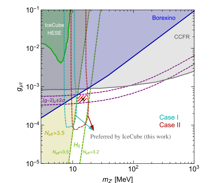
We show in Fig. 4 the preferred regions by IceCube we find in this work in the mass-coupling plane, accompanied by the excluded region by the CCFR experiment Mishra et al. 1991 (gray shaded region), the blue shaded region is the excluded region by Borexino Bellini et al. 2011, while the purple band represents the preferred region from the discrepancy Amaral et al. 2021. It is also important to note that such leptophilic interactions mentioned in this work can also affect the relativistic degrees of freedom of neutrinos and so to avoid tension with cosmology it requires that MeV so that Escudero et al. 2019. We show the excluded region in yellow. It was also mentioned in Ref. Escudero et al. 2019 that an additional boson can also alleviate the Hubble tension (even though it cannot be fully resolved), for the mass-coupling region shown with the green band. Last but not least, one could see all the favored regions cross each other at MeV and , shown in the hashed red region. Note that the cosmological limit used here considers the kinetic mixing, which is stronger than limits only with neutrino self-interactions although it depends on van den Aarssen et al. 2012; Ahlgren et al. 2013; Kamada and Yu 2015.
The preferred regions are intriguing because results obtained from three independent measurements meet each other. On the other hand, we stress that the IceCube data have not shown evidence for secret neutrino self-interactions, by which we can place an upper limit on the coupling rather than the preferred region. We also show the previous results by Ref. Bustamante et al. 2020 in Fig. 4. The constraints are weaker than the limits from Borexino as well as other laboratory experiments such as the kaon-decay measurement implying Blum et al. 2014.
IV Future Prospects
Lastly, we consider the impact of next-generation detectors such as IceCube-Gen2 Aartsen et al. 2020b on the gauged scenario considered in this work. In particular, we are interested in the unique parameter space, where the muon anomaly solution, Hubble tension alleviation, and IceCube preferred region are overlapping. For demonstration, we adopt MeV and as the fiducial scenario (shown as the black cross in Fig. 3). Using the zenith-angle-averaged effective areas for shower-type events based on Fig. 25 from Ref. Aartsen et al. 2020b we estimate the number of events coming from a given neutrino flux. As in the analysis in the previous section, this approach here is different from those in Refs. Blum et al. 2014; Shoemaker and Murase 2016 that used the energy deposited in the detector. In Fig. 5 we compare neutrino spectra with and without BSM neutrino-neutrino scatterings in red and black data points respectively, assuming 10 years of IceCube-Gen2 data and the neutrino spectrum with and . It shows that with statistics expected in IceCube-Gen2, the dip feature will be evident if it exists. We also compute the resulting , and find that our fiducial scenario would be discrepant with the SM case without secret interactions. Although results depend on our understanding of astrophysical components, this demonstrates that such model can be probed by the IceCube telescopes.
In Fig. 5, only statistical errors are considered. In reality, there are other systematics, which need to be taken into account. As noted above, the deposited energy is smaller than the neutrino energy, which can make the expected dip broader. The atmospheric background gives additional systematics in the analysis. On the other hand, this analysis only used the shower data. Muon track data including starting and through-going events should also give us information. One may be able to further uncover the nature of the preferred model of secret self-interactions by combining spectral and flavor modifications Shoemaker and Murase 2016; Barenboim et al. 2019, and global analyses as in Ref. Aartsen et al. 2015 will be more powerful.
V Summary and Discussion
It has been suggested that the gauged model accounts for the muon anomaly. High-energy neutrino data provide an independent test for this model through dip signatures caused by secret neutrino self-interactions. We showed in this work that the current 6-yr shower data of IceCube prefers couplings and masses consistent with the Muon data, which also overlaps with the parameter space alleviating the Hubble tension Escudero et al. 2019.
We have performed a likelihood analysis similar to ref. Aartsen et al. 2020c, where we show our results based on the assumption that the gauged model is “preferred” over the null hypothesis. This is because the current IceCube shower data have a paucity in the PeV range, but the sensitivity (or constraint) is weaker as indicated by the HESE constraint in Fig. 4. Gen2 can be sensitive to the preferred region hinted by ICeCube.
Future neutrino experiments such as IceCube-Gen2 will be sensitive to the parameter space indicated by Fig. 5, and may confirm the dip. But one should keep in mind that the dip can also be caused by astrophysical sources. For example, this may reflect two or more astrophysical populations Chen et al. 2015; Murase et al. 2016. The dip could also be caused by the Bethe-Heitler process that can be important between and interactions and/or the combination of multi-pion production and pileup due to the meson/muon cooling. However, these details are model dependent, and it is beyond the scope of this work to perform the BSM analysis taking account of such astrophysical systematics.
If this result is confirmed, the combination of the data may not only reveal the existence of a new fundamental symmetry, but also uncover the neutrino mass spectrum. We found that the required parameter space is narrow, and the total neutrino mass has to range from 0.06 eV to 0.3 eV. This is also encouraging for future neutrino mass measurements (e.g., Abazajian et al. 2016; Dvorkin et al. 2019; Betti et al. 2019; Ashtari Esfahani et al. 2017).
We also demonstrated that the gauged scenario for the muon anomaly and Hubble tension alleviation can critically be tested by IceCube-Gen2. This result is consistent with the previous work that showed next-generation neutrino telescopes can reach the limit expected in the mean free path limit Shoemaker and Murase 2016.
Another important test with high-energy neutrinos is to utilize multimessenger observations from individual neutrino sources Kelly and Machado 2018; Murase and Shoemaker 2019; Koren 2019. In particular, BSM neutrino echoes – delayed neutrino emission through secret neutrino-neutrino scatterings provide a test that is insensitive to the unknown astrophysical spectrum. Ref. Murase and Shoemaker 2019 showed that IceCube-Gen2 can reach for the vector mediator scenario.
Acknowledgements.
The work of K.M. is supported by the NSF Grant No. AST-1908689, No. AST-2108466 and No. AST-2108467, and KAKENHI No. 20H01901 and No. 20H05852. The work of I.M.S. and Z.T. is supported by the U.S. Department of Energy under the award number DE-SC0020250. Z.T. appreciates the useful discussions with Joachim Kopp.
Appendix A Cascades Effects
In order to confirm that the up- scattering of neutrinos does not affect the analysis of this work we have made Fig. 6. To get the ”no cascade” plot, we have collected all the particles that never scattered. As it should be expected the ”no cascade” case is always below the cascade one, because in the latter we are still getting some energy deposited between resonances from scattered particles. However, the difference is about a factor of two at the peak located between resonances, and it does not significantly affect the preferred region we have obtained in this analysis.
References
- Abi et al. (2021) B. Abi et al. (Muon g-2), Phys. Rev. Lett. 126, 141801 (2021), eprint 2104.03281.
- Bennett et al. (2006) G. W. Bennett et al. (Muon g-2), Phys. Rev. D 73, 072003 (2006), eprint hep-ex/0602035.
- Davier et al. (2011) M. Davier, A. Hoecker, B. Malaescu, and Z. Zhang, Eur. Phys. J. C 71, 1515 (2011), [Erratum: Eur.Phys.J.C 72, 1874 (2012)], eprint 1010.4180.
- Davier et al. (2017) M. Davier, A. Hoecker, B. Malaescu, and Z. Zhang, Eur. Phys. J. C77, 827 (2017), eprint 1706.09436.
- Davier et al. (2020) M. Davier, A. Hoecker, B. Malaescu, and Z. Zhang, Eur. Phys. J. C80, 241 (2020), [Erratum: Eur. Phys. J. C80, 410 (2020)], eprint 1908.00921.
- Borsanyi et al. (2021) S. Borsanyi et al., Nature (2021), eprint 2002.12347.
- Zhang et al. (2022) H.-B. Zhang, C.-X. Liu, J.-L. Yang, and T.-F. Feng, Chin. Phys. C 46, 093107 (2022), eprint 2104.03489.
- Baum et al. (2022) S. Baum, M. Carena, N. R. Shah, and C. E. M. Wagner, JHEP 01, 025 (2022), eprint 2104.03302.
- Ahmed et al. (2022) W. Ahmed, I. Khan, J. Li, T. Li, S. Raza, and W. Zhang, Phys. Lett. B 827, 136879 (2022), eprint 2104.03491.
- Cox et al. (2021) P. Cox, C. Han, and T. T. Yanagida, Phys. Rev. D 104, 075035 (2021), eprint 2104.03290.
- Abdughani et al. (2021) M. Abdughani, Y.-Z. Fan, L. Feng, Y.-L. S. Tsai, L. Wu, and Q. Yuan, Sci. Bull. 66, 2170 (2021), eprint 2104.03274.
- Van Beekveld et al. (2021) M. Van Beekveld, W. Beenakker, M. Schutten, and J. De Wit, SciPost Phys. 11, 049 (2021), eprint 2104.03245.
- Yin (2021) W. Yin, JHEP 06, 029 (2021), eprint 2104.03259.
- Han (2021) C. Han (2021), eprint 2104.03292.
- Buen-Abad et al. (2021) M. A. Buen-Abad, J. Fan, M. Reece, and C. Sun, JHEP 09, 101 (2021), eprint 2104.03267.
- Wang et al. (2021a) F. Wang, L. Wu, Y. Xiao, J. M. Yang, and Y. Zhang, Nucl. Phys. B 970, 115486 (2021a), eprint 2104.03262.
- Cao et al. (2021) J. Cao, J. Lian, Y. Pan, D. Zhang, and P. Zhu, JHEP 09, 175 (2021), eprint 2104.03284.
- Gu et al. (2021) Y. Gu, N. Liu, L. Su, and D. Wang, Nucl. Phys. B 969, 115481 (2021), eprint 2104.03239.
- Athron et al. (2021) P. Athron, C. Balázs, D. H. J. Jacob, W. Kotlarski, D. Stöckinger, and H. Stöckinger-Kim, JHEP 09, 080 (2021), eprint 2104.03691.
- Aboubrahim et al. (2021) A. Aboubrahim, M. Klasen, and P. Nath, Phys. Rev. D 104, 035039 (2021), eprint 2104.03839.
- Yang et al. (2021) J.-L. Yang, H.-B. Zhang, C.-X. Liu, X.-X. Dong, and T.-F. Feng, JHEP 08, 086 (2021), eprint 2104.03542.
- Greljo et al. (2021) A. Greljo, P. Stangl, and A. E. Thomsen, Phys. Lett. B 820, 136554 (2021), eprint 2103.13991.
- Zu et al. (2022) L. Zu, X. Pan, L. Feng, Q. Yuan, and Y.-Z. Fan, JCAP 08, 028 (2022), eprint 2104.03340.
- Cadeddu et al. (2021) M. Cadeddu, N. Cargioli, F. Dordei, C. Giunti, and E. Picciau, Phys. Rev. D 104, 011701 (2021), eprint 2104.03280.
- Kawamura and Raby (2021) J. Kawamura and S. Raby, Phys. Rev. D 104, 035007 (2021), eprint 2104.04461.
- Li et al. (2021a) T. Li, M. A. Schmidt, C.-Y. Yao, and M. Yuan, Eur. Phys. J. C 81, 811 (2021a), eprint 2104.04494.
- Borah et al. (2021) D. Borah, M. Dutta, S. Mahapatra, and N. Sahu, Phys. Lett. B 820, 136577 (2021), eprint 2104.05656.
- Buras et al. (2021) A. J. Buras, A. Crivellin, F. Kirk, C. A. Manzari, and M. Montull, JHEP 06, 068 (2021), eprint 2104.07680.
- Arcadi et al. (2021) G. Arcadi, L. Calibbi, M. Fedele, and F. Mescia (2021), eprint 2104.03228.
- Bai and Berger (2021) Y. Bai and J. Berger (2021), eprint 2104.03301.
- Lu et al. (2021) C.-T. Lu, R. Ramos, and Y.-L. S. Tsai, JHEP 08, 073 (2021), eprint 2104.04503.
- Ge et al. (2021) S.-F. Ge, X.-D. Ma, and P. Pasquini, Eur. Phys. J. C 81, 787 (2021), eprint 2104.03276.
- Brdar et al. (2021) V. Brdar, S. Jana, J. Kubo, and M. Lindner, Phys. Lett. B 820, 136529 (2021), eprint 2104.03282.
- Ferreira et al. (2021) P. M. Ferreira, B. L. Gonçalves, F. R. Joaquim, and M. Sher, Phys. Rev. D 104, 053008 (2021), eprint 2104.03367.
- Wang et al. (2021b) H.-X. Wang, L. Wang, and Y. Zhang, Eur. Phys. J. C 81, 1007 (2021b), eprint 2104.03242.
- Chen et al. (2021) J. Chen, Q. Wen, F. Xu, and M. Zhang (2021), eprint 2104.03699.
- Chun and Mondal (2021) E. J. Chun and T. Mondal, JHEP 07, 044 (2021), eprint 2104.03701.
- Arcadi et al. (2022) G. Arcadi, A. S. de Jesus, T. B. de Melo, F. S. Queiroz, and Y. S. Villamizar, Nucl. Phys. B 982, 115882 (2022), eprint 2104.04456.
- Li et al. (2021b) T. Li, J. Pei, and W. Zhang, Eur. Phys. J. C 81, 671 (2021b), eprint 2104.03334.
- Escribano et al. (2021) P. Escribano, J. Terol-Calvo, and A. Vicente, Phys. Rev. D 103, 115018 (2021), eprint 2104.03705.
- Coluccio Leskow et al. (2017) E. Coluccio Leskow, G. D’Ambrosio, A. Crivellin, and D. Müller, Phys. Rev. D 95, 055018 (2017), eprint 1612.06858.
- Crivellin et al. (2021) A. Crivellin, D. Mueller, and F. Saturnino, Phys. Rev. Lett. 127, 021801 (2021), eprint 2008.02643.
- He et al. (1991a) X. G. He, G. C. Joshi, H. Lew, and R. R. Volkas, Phys. Rev. D 43, 22 (1991a).
- He et al. (1991b) X.-G. He, G. C. Joshi, H. Lew, and R. R. Volkas, Phys. Rev. D 44, 2118 (1991b).
- Altmannshofer et al. (2014a) W. Altmannshofer, S. Gori, M. Pospelov, and I. Yavin, Phys. Rev. D 89, 095033 (2014a), eprint 1403.1269.
- Altmannshofer et al. (2014b) W. Altmannshofer, S. Gori, M. Pospelov, and I. Yavin, Phys. Rev. Lett. 113, 091801 (2014b), eprint 1406.2332.
- Bauer et al. (2018) M. Bauer, P. Foldenauer, and J. Jaeckel, JHEP 07, 094 (2018), eprint 1803.05466.
- Amaral et al. (2021) D. W. P. Amaral, D. G. Cerdeño, A. Cheek, and P. Foldenauer (2021), eprint 2104.03297.
- Kahn et al. (2018) Y. Kahn, G. Krnjaic, N. Tran, and A. Whitbeck, JHEP 09, 153 (2018), eprint 1804.03144.
- Galon et al. (2020) I. Galon, E. Kajamovitz, D. Shih, Y. Soreq, and S. Tarem, Phys. Rev. D 101, 011701 (2020), eprint 1906.09272.
- Ioka and Murase (2014) K. Ioka and K. Murase, PTEP 2014, 061E01 (2014), eprint 1404.2279.
- Ng and Beacom (2014) K. C. Y. Ng and J. F. Beacom, Phys. Rev. D 90, 065035 (2014), [Erratum: Phys.Rev.D 90, 089904 (2014)], eprint 1404.2288.
- Cyr-Racine and Sigurdson (2014) F.-Y. Cyr-Racine and K. Sigurdson, Phys. Rev. D 90, 123533 (2014), eprint 1306.1536.
- Archidiacono and Hannestad (2014) M. Archidiacono and S. Hannestad, JCAP 07, 046 (2014), eprint 1311.3873.
- Lancaster et al. (2017) L. Lancaster, F.-Y. Cyr-Racine, L. Knox, and Z. Pan, JCAP 07, 033 (2017), eprint 1704.06657.
- Oldengott et al. (2017) I. M. Oldengott, T. Tram, C. Rampf, and Y. Y. Y. Wong, JCAP 11, 027 (2017), eprint 1706.02123.
- Kreisch et al. (2020) C. D. Kreisch, F.-Y. Cyr-Racine, and O. Doré, Phys. Rev. D 101, 123505 (2020), eprint 1902.00534.
- Blinov et al. (2019) N. Blinov, K. J. Kelly, G. Z. Krnjaic, and S. D. McDermott, Phys. Rev. Lett. 123, 191102 (2019), eprint 1905.02727.
- Weinberg (2013) S. Weinberg, Phys. Rev. Lett. 110, 241301 (2013), eprint 1305.1971.
- Berlin and Blinov (2019) A. Berlin and N. Blinov, Phys. Rev. D 99, 095030 (2019), eprint 1807.04282.
- D’Eramo et al. (2018) F. D’Eramo, R. Z. Ferreira, A. Notari, and J. L. Bernal, JCAP 11, 014 (2018), eprint 1808.07430.
- Escudero et al. (2019) M. Escudero, D. Hooper, G. Krnjaic, and M. Pierre, JHEP 03, 071 (2019), eprint 1901.02010.
- Araki et al. (2015) T. Araki, F. Kaneko, Y. Konishi, T. Ota, J. Sato, and T. Shimomura, Phys. Rev. D 91, 037301 (2015), eprint 1409.4180.
- Kamada and Yu (2015) A. Kamada and H.-B. Yu, Phys. Rev. D 92, 113004 (2015), eprint 1504.00711.
- DiFranzo and Hooper (2015) A. DiFranzo and D. Hooper, Phys. Rev. D 92, 095007 (2015), eprint 1507.03015.
- Farzan (2015) Y. Farzan, Phys. Lett. B 748, 311 (2015), eprint 1505.06906.
- Denton et al. (2018) P. B. Denton, Y. Farzan, and I. M. Shoemaker, JHEP 07, 037 (2018), eprint 1804.03660.
- Okada and Seto (2020) N. Okada and O. Seto, Phys. Rev. D 101, 023522 (2020), eprint 1908.09277.
- Aartsen et al. (2020a) M. G. Aartsen et al. (IceCube), Phys. Rev. Lett. 125, 121104 (2020a), eprint 2001.09520.
- Aghanim et al. (2020) N. Aghanim et al. (Planck), Astron. Astrophys. 641, A6 (2020), [Erratum: Astron.Astrophys. 652, C4 (2021)], eprint 1807.06209.
- Mishra et al. (1991) S. R. Mishra et al. (CCFR), Phys. Rev. Lett. 66, 3117 (1991).
- Harnik et al. (2012) R. Harnik, J. Kopp, and P. A. N. Machado, JCAP 07, 026 (2012), eprint 1202.6073.
- Bellini et al. (2011) G. Bellini et al., Phys. Rev. Lett. 107, 141302 (2011), eprint 1104.1816.
- Blum et al. (2014) K. Blum, A. Hook, and K. Murase (2014), eprint 1408.3799.
- Cherry et al. (2014) J. F. Cherry, A. Friedland, and I. M. Shoemaker (2014), eprint 1411.1071.
- Cherry et al. (2016) J. F. Cherry, A. Friedland, and I. M. Shoemaker (2016), eprint 1605.06506.
- Ibe and Kaneta (2014) M. Ibe and K. Kaneta, Phys.Rev. D90, 053011 (2014), eprint 1407.2848.
- Creque-Sarbinowski et al. (2021) C. Creque-Sarbinowski, J. Hyde, and M. Kamionkowski, Phys. Rev. D 103, 023527 (2021), eprint 2005.05332.
- Murase et al. (2016) K. Murase, D. Guetta, and M. Ahlers, Phys. Rev. Lett. 116, 071101 (2016), eprint 1509.00805.
- Yuksel et al. (2008) H. Yuksel, M. D. Kistler, J. F. Beacom, and A. M. Hopkins, Astrophys. J. Lett. 683, L5 (2008), eprint 0804.4008.
- Shoemaker and Murase (2016) I. M. Shoemaker and K. Murase, Phys. Rev. D 93, 085004 (2016), eprint 1512.07228.
- Abbasi et al. (2020) R. Abbasi et al. (IceCube) (2020), eprint 2011.03545.
- Murase and Waxman (2016) K. Murase and E. Waxman, Phys. Rev. D94, 103006 (2016), eprint 1607.01601.
- Murase (2007) K. Murase, Phys.Rev. D76, 123001 (2007), eprint 0707.1140.
- Bustamante et al. (2020) M. Bustamante, C. Rosenstrøm, S. Shalgar, and I. Tamborra, Phys. Rev. D 101, 123024 (2020), eprint 2001.04994.
- van den Aarssen et al. (2012) L. G. van den Aarssen, T. Bringmann, and C. Pfrommer, Phys. Rev. Lett. 109, 231301 (2012), eprint 1205.5809.
- Ahlgren et al. (2013) B. Ahlgren, T. Ohlsson, and S. Zhou, Phys. Rev. Lett. 111, 199001 (2013), eprint 1309.0991.
- Aartsen et al. (2020b) M. G. Aartsen et al. (IceCube-Gen2) (2020b), eprint 2008.04323.
- Barenboim et al. (2019) G. Barenboim, P. B. Denton, and I. M. Oldengott, Phys. Rev. D 99, 083515 (2019), eprint 1903.02036.
- Aartsen et al. (2015) M. G. Aartsen et al. (IceCube Collaboration), Astrophys. J. 809, 98 (2015), eprint 1507.03991.
- Aartsen et al. (2020c) M. G. Aartsen et al. (IceCube), Phys. Rev. Lett. 125, 141801 (2020c), eprint 2005.12942.
- Chen et al. (2015) C.-Y. Chen, P. S. Bhupal Dev, and A. Soni, Phys. Rev. D92, 073001 (2015), eprint 1411.5658.
- Abazajian et al. (2016) K. N. Abazajian et al. (CMB-S4) (2016), eprint 1610.02743.
- Dvorkin et al. (2019) C. Dvorkin et al. (2019), eprint 1903.03689.
- Betti et al. (2019) M. G. Betti et al. (PTOLEMY), JCAP 07, 047 (2019), eprint 1902.05508.
- Ashtari Esfahani et al. (2017) A. Ashtari Esfahani et al. (Project 8), J. Phys. G 44, 054004 (2017), eprint 1703.02037.
- Kelly and Machado (2018) K. J. Kelly and P. A. N. Machado, JCAP 1810, 048 (2018), eprint 1808.02889.
- Murase and Shoemaker (2019) K. Murase and I. M. Shoemaker, Phys. Rev. Lett. 123, 241102 (2019), eprint 1903.08607.
- Koren (2019) S. Koren, JCAP 09, 013 (2019), eprint 1903.05096.