Using brain inspired principles to unsupervisedly learn good representations for visual pattern recognition

Luis Sa-Couto luis.sa.couto@tecnico.ulisboa.pt Address: Department of Computer Science and Engineering, INESC-ID & Instituto Superior Técnico University of Lisbon, Av. Prof. Dr. Aníbal Cavaco Silva, 2744-016 Porto Salvo, Portugal Andreas Wichert andreas.wichert@tenico.ulisboa.pt

Abstract

Although deep learning has solved difficult problems in visual pattern recognition, it is mostly successful in tasks where there are lots of labeled training data available. Furthermore, the global back-propagation based training rule and the amount of employed layers represents a departure from biological inspiration. The brain is able to perform most of these tasks in a very general way from limited to no labeled data. For these reasons it is still a key research question to look into computational principles in the brain that can help guide models to unsupervisedly learn good representations which can then be used to perform tasks like classification. In this work we explore some of these principles to generate such representations for the MNIST data set. We compare the obtained results with similar recent works and verify extremely competitive results.

keywords

Hubel Wiesel’s Hypothesis ,Brain inspired architectures ,Invariant Pattern Recognition ,Deep Learning

^†^†titlenote: This work was supported by national funds through Fundação para a Ciência e Tecnologia (FCT) with reference UID/CEC/50021/2020 and through doctoral grant SFRH/BD/144560/2019 awarded to the first author. The funders had no role in study design, data collection and analysis, decision to publish, or preparation of the manuscript. The authors declare no conflicts of interest.^†^†corresponding: Corresponding author

1 Introduction

Deep Learning is now regarded as the main paradigm to solve most learning problems in natural tasks like vision Goodfellow et al. 2016. And rightfully so since the results on many tasks have been astounding Krizhevsky et al. 2017. Yet, this is mainly the case when large sets of labeled data are available. Although there was some inspiration at the beginning McCulloch and Pitts 1943; Rosenblatt 1958; Rumelhart et al. 1986; Fukushima 1980; Lecun and Bengio 1995, the Deep Learning approach has mainly departed from brain related principles. However, the brain is the best natural example of a learning system that can perform extremely difficult tasks in a mostly unsupervised manner Trappenberg 2009. For that reason, it is still a relevant and active area of research to look into some established computational brain principles to help guide the development of different models that can unsupervisedly learn useful representations to solve difficult tasks Hawkins et al. 2016; Poggio et al. 2016; Illing et al. 2019; Balaji Ravichandran et al. 2020; George et al. 2017; Sa-Couto and Wichert 2019; George et al. 2020. Due to the lack of a well established theoretical understanding of the brain one can be overwhelmed by the tons of separate pieces of information related to it. To this end, it is helpful to recall Marr’s three levels Marr 2010 and abstract away much of the complexity that can come from specific neural implementations and networks. In this work, much like in George et al. 2020, we try to identify some key computational principles and constraints which are established about how the brain processes visual data and implement them in a model such that it is able to build useful unsupervised representations of simple images. Therefore, we structure the paper around four key principles:

1.

What-where separation of information: since early experiments on the early layers of the visual cortex Hubel and Wiesel 1962; Hubel and Wiesel 1968 that there is evidence for structures that are specific to identify particular stimuli (what) and others that are modelers of position (where).
2.

Locality of learning: due to physical limitations, study on how the brain learns points to the locality of the updates Hebb 1949; Sejnowski and Tesauro 1989; Hertz et al. 1991; Trappenberg 2009; Illing et al. 2019.
3.

Vision is a temporal task: although most machine learning approaches to image data use the pixel matrix as a fixed input, it is well established that the brain processes vision through time with the eyes changing position Liversedge and Findlay 2000; Hawkins et al. 2016.
4.

The central area of the retina (i.e. the fovea) has a detailed view of the image, while outer areas have only a blurred view Haekness and Bennet-Clark 1978.

We use section 2 to further detail these principles and how they have appeared in the literature. Then, we use section 3 to provide a detailed description of how our proposed model aims to implement the principles. Section 4 not only presents an empirical view of the model and on how to choose the hyper-parameters, but also applies the typical experiment applied in similar works Balaji Ravichandran et al. 2020; Illing et al. 2019 using the MNIST LeCun et al. data set. Finally, we conclude the paper in section 5 with some take aways and outlining some possible paths forward.

2 The principles in the literature

Hubel and Wiesel’s experiments on the early stages of the visual cortex found two specific types of cells named simple and complex Hubel and Wiesel 1962; Hubel and Wiesel 1968; Hubel 1988; Trappenberg 2009. Simple cells are tuned to specific stimuli like oriented lines. One might say that they are concerned about modeling what the input is. On the other hand, complex cells seem to react to the same stimuli but allowing for shifts in position. These cells can be seen as modeling the positional information of where the stimulus occurs. This idea of first modeling the “what” of the stimulus and then modeling the “where” of that same stimulus inspired many learning architectures for visual pattern recognition. The seminal Neocognitron Fukushima 1980 tried to implement Hubel and Wiesel’s discoveries almost directly. This model then led to a few generalizations Cardoso and Wichert 2010 and improvements Fukushima 2003 to increase performance. In a very biologically inspired implementation of the same principles the well-known HMAX approach was proposed Riesenhuber and Poggio 1999 and succeeded on several tasks Serre et al. 2007, which led to increased interest in it with several developments and new versions Hu et al. 2014; Poggio et al. 2016. A parallel path, took the Neocognitron and departed from biological realism to achieve the powerful engineering tool of convolution networks Lecun and Bengio 1995; LeCun et al. 1998. With increasing computational power and many advances in the Deep Learning approach to train large networks, convolution networks became the most successful member of this family at solving hard tasks Goodfellow et al. 2016; Krizhevsky et al. 2017. With all of that it seems that there may be something helpful about this principle and, for that reason, we will use it to guide the development of the proposed model.

Although back-propagation of gradients is the key approach behind learning successful deep networks, the biological plausibility of such dependences is questionable Trappenberg 2009. In fact, neuroscience literature seems to point to local learning rules that are inspired by Hebb’s hypotheses Hebb 1949; Sejnowski and Tesauro 1989. For that reason, a lot of research effort has been put into developing alternative learning schemes that work layer-wise Sandberg et al. 2002; Balaji Ravichandran et al. 2020; Illing et al. 2019. With that, we will build a model in a way that all learning requires only local information from consecutive layers.

Most machine learning approaches to image data use the pixel matrix as a fixed input Lecun and Bengio 1995; Krizhevsky et al. 2017. However, it is well established that the brain processes vision through time with the eyes changing position. For instance, there is extremely interesting literature around the role that saccadic eye movements play in recognition Liversedge and Findlay 2000. With that, we will follow the lines of related research Hawkins et al. 2016 and include a time component in our processing.

At a given moment in time, the image that is projected in the retina is described at different resolutions. More specifically, the central area of the retina (i.e. the fovea) has a detailed view of the image, while outer areas have only a blurred view Haekness and Bennet-Clark 1978. It is often posited that the central area can focus on detail while the outer areas offer the context where the detail is inserted. In our opinion, this view, combined with further neuroscientific evidence, suggests that the brain may use outer retinal information to have a notion about the relative position of the detail in the object. This led us to posit an object-dependent frame in previous work on developing sparse codes for an associative memory task Sa-Couto and Wichert 2019 and for classification Sa-Couto and Wichert 2020. In this paper we will further detail this idea and include this kind of processing in our model.

3 Putting the principles in a model

Following the aforementioned third and fourth principles, we define an $f\times f$ sized window that represents the high detailed region of the model’s view of the image at a particular time step. We can look at the content of this region as a vector $\mathbf{x}_{what}$ . Furthermore, we use the outer area’s information to find the position of this content window in an object-dependent coordinate system (we will see later how). We can look at this position as a vector $\mathbf{x}_{where}$ . This logic is illustrated in figure 1.

With that, at each moment in time we get two pieces of information. Following the what-where principle, and looking at figure 1 for an illustration, the model starts by processing $\mathbf{x}_{what}$ . To that end, there is a what layer, which will be detailed in subsection 3.1. This layer performs recognition of the content and directs processing to a where layer that is specific for that type of stimulus. As the name indicates, the where layer models the positional information $\mathbf{x}_{where}$ and will also be detailed later (in subsection 3.2).

From this abstract view of the model, we can see that, for each time step, we will generate a vector that encodes information about what was seen and where it was seen relative to the global object. To get at a single, final representation for the whole object we will need to combine all of these vectors into one. We will discuss our approach to this issue in subsection 3.3.

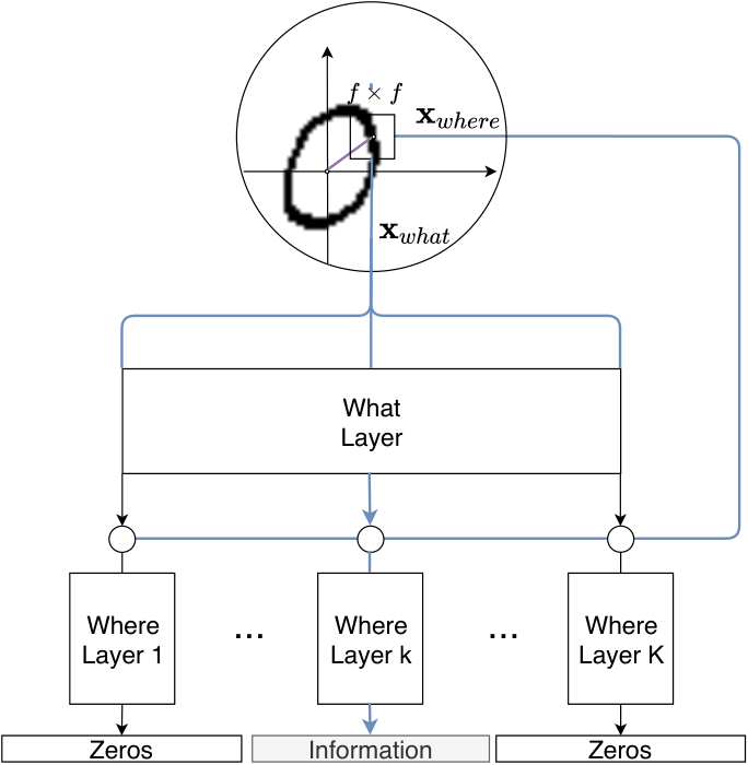
Refer to caption — Figure 1: At a given instant, an $f\times f$ window $\mathbf{x}_{what}$ of the image is taken as input to the what layer. The what layer then identifies the where layer that corresponds to this particular input. That where layer receives as input the window’s object-dependent position $\mathbf{x}_{where}$ and based on that provides an encoding of the information. Looking at the output as a vector, we can say that all where layers that were not chosen by the what layer provide an output of zeros while the chosen layer provides an encoding for the information.

3.1 What

In this subsection we open the abstract “what layer” box in figure 1. Besides describing its operation we also detail which hyper-parameters are involved and how to learn the trainable parameters.

3.1.1 Feature Mapping

The what layer implements the winner takes all approach to feature mapping Cardoso and Wichert 2010. Each of $K$ units is tuned to recognize a given preferred pattern $\mathbf{w}_{k},k=1,\ldots,K$ (like a corner or an oriented line). Given an input, each unit measures a cosine similarity between its preferred pattern and that input Sa-Couto and Wichert 2019. The usage of this measure can be viewed as applying weight normalization in a typical dot product based layer. Such normalization is also biologically plausible since synaptic strength cannot grow unbounded Hertz et al. 1991; Trappenberg 2009. The units then compete and the most similar one wins firing a $1$ while the others output $0$ . The usage of an absolute minimum threshold $T$ ensures that there is not always a winner. For inputs that do not resemble any of the preferred patterns, all units will be silent.

To implement this reasoning, we write the net input to unit $k$ with equation 1.

net_{k}=\frac{\mathbf{x}_{what}^{T}\mathbf{w}_{k}}{\left\|\mathbf{x}_{what}^{T}\right\|\left\|\mathbf{w}_{k}\right\|}

(1)

To define the binary activations of each unit we use the well-known, right continuous, Heaviside step activation function given in equation 2.

H^{{}^{+}}\left(x\right)=\begin{cases}1&x\geq 0\\ 0&x<0\end{cases}

(2)

Unit $k$ ’s output, written $what_{k}$ , is the result of the competition between the layer’s units and it can be written with equation 3.

what_{k}=H^{+}\left(net_{k}-\max\left(T,\max_{l\in\left\{1,\cdots,K\right\}}net_{l}\right)\right)

(3)

Figure 2 provides an illustration of information processing in the what layer.

Figure 2: The what layer implements the winner takes all approach to feature mapping. Each of

K

units is tuned to recognize a given preferred pattern

\mathbf{w}

(like a corner or an oriented line). Given an input, each unit measures a cosine similarity between its preferred pattern and that input. The units then compete and the most similar one wins firing a

1

while the others output

0

. The usage of an absolute minimum threshold

T

ensures that there is not always a winner. For inputs that do not resemble any of the preferred patterns, all units will be silent.

3.1.2 Competitive Learning

Now that we have described the operation we are left with the learning problem: how to learn the preferred patterns $\mathbf{w}_{k}$ ? To this end we employ the typical competitive learning approach Rumelhart and Zipser 1985; Hertz et al. 1991; Haykin 2008 where for a given input, the winner unit gets its weights updated. One can also look at this learning approach as a variant of k-means clustering Lloyd 1982 applied in a stochastic manner to minibatches Sculley 2010. All in all, we can describe the learning procedure with the rule in equation 4 where $\eta_{k}$ is the learning rate.

\mathbf{w}_{k}=\mathbf{w}_{k}+what_{k}\eta_{k}\left(\mathbf{x}_{p}-\mathbf{w}_{k}\right)

(4)

Besides adjusting the learnable parameters, $T$ , $K$ and $f$ play the role of hyper-parameters and have to be chosen based on the task at hand. In section 4 we will discuss how we chose them for specific experiments.

3.2 Where

In this subsection we open one of the abstract “where layer” boxes in figure 1. Besides describing its operation we also detail which hyper-parameters are involved an how to learn the trainable parameters. In general, we can describe the operation of this layer as using a Gaussian Mixture Model Bishop 2006; Murphy 2012 of positions in the object-dependent space.

3.2.1 Object dependent frame

The first important issue comes in the definition of the object-dependent frame. Assuming that $\mathbf{x}_{img}$ corresponds to the window’s position in the pixel matrix. To transform this position to the new coordinate system we need a center and a radius. To compute them, we need to know which positions belong to the object. In a more realistic scenario, one could use stereopsis and depth combined with color to achieve this (or even a segmentation model). However, since this is not the main point of this work, we abstract away this complexity and use the same strategy as in Sa-Couto and Wichert 2019; Sa-Couto and Wichert 2020 and state that a position belongs to the object if its what layer activation is nonzero. Using that strategy, we can use equation 5 to compute the center

C=\frac{\sum_{\mathbf{x}_{img}}\sum_{k=1}^{K}\mathbf{x}_{img}what_{k}\left(\mathbf{x}_{img}\right)}{\sum_{\mathbf{x}_{img}}\sum_{k=1}^{K}what_{k}\left(\mathbf{x}_{img}\right)}

(5)

and equation 6 to compute the radius.

R=\max_{\mathbf{x}_{img},k\in\left\{1,\ldots,K\right\}}\left\{what_{k}\left(\mathbf{x}_{img}\right)\left\|\mathbf{x}_{img}-C\right\|_{2}\right\}

(6)

With that, we can map $\mathbf{x}_{img}$ to the intended $\mathbf{x}_{where}$ using equation 7.

\mathbf{x}_{where}=\frac{\mathbf{x}_{img}-C}{R}

(7)

3.2.2 Positional Mapping

To implement the Gaussian mixture, each unit $l\in\left\{1,\ldots,C_{k}\right\}$ in where layer $k$ is parameterized by a weight $\pi_{l}^{k}$ , a center $\mu_{l}^{k}$ and a covariance $\mathbf{\Sigma}_{l}^{k}$ . The net input to a unit is the unnormalized Gaussian probability assigned by that unit to that particular position. This is expressed in equation 8.

net_{l}^{k}=\pi_{l}^{k}\mathcal{N}\left(\mathbf{x}_{where}\mid\mathbf{\mu}_{l}^{k},\mathbf{\Sigma}_{l}^{k}\right)

(8)

One can interpret the mean and covariance as describing a receptive field over positions.

The final output of each unit is also the product of competition between lateral units as is written in equation 9. This is basically the normalization of the probabilities.

where_{l}^{k}=\frac{net_{l}}{\sum_{i=1}^{C_{k}}net_{i}}

(9)

With this description, we see that, since each unit represents a component, the layer’s operations is a competition to see from which component the position was generated. Figure 3 provides an illustration of the layer’s operation.

Figure 3: Where layer

k

has

C_{k}

units that describe a Gaussian mixture over the space of object-dependent positions of occurrences of a given pattern. Each unit has a weight, a mean vector and a covariance that together describe the area of frequently occurring positions. The final output is a soft competition to decide which component generated the observed position.

3.2.3 Expectation Maximization Learning

To learn the parameters we apply the typical approach to learn a Gaussian Mixture. More specifically, we use expectation-maximization Bishop 2006. For a set of $P$ examples, the expectation step corresponds to computing the layer’s output for each one. The maximization step is just the maximum likelihood estimation of each parameter using equations 10, 11 and 12.

\mu_{l}^{k}=\frac{1}{\sum_{p=1}^{P}where_{pl}^{k}}\sum_{p=1}^{P}where_{pl}^{k}\mathbf{x}_{p}

(10)

\Sigma_{l}^{k}=\frac{1}{\sum_{p=1}^{P}where_{pl}^{k}}\sum_{p=1}^{P}where_{pl}^{k}\left(\mathbf{x}_{p}-\mathbf{\mu}_{l}^{k}\right)\left(\mathbf{x}_{p}-\mathbf{\mu}_{l}^{k}\right)^{T}

(11)

\pi_{l}^{k}=\frac{\sum_{p=1}^{P}where_{pl}^{k}}{\sum_{p=1}^{P}\sum_{l^{\prime}=1}^{C_{k}}where_{pl^{\prime}}^{k}}

(12)

Besides the learnable parameters, it is a key architectural feature to decide how many units each where layer uses. In section 4 we will use a heuristic way of making this decision for a specific task.

Now that we have lifted the lids from the abstracted view in figure 1 we can put it all together in a detailed view (see figure 4) of the processing at a given time step.

3.3 Pooling Sparse Views to get a global view

As we have stated before, with a vector description for each time step we need a way to combine all descriptions into a final one. To get a probabilistic presence map telling wether a given feature has appeared at a given position or not, it makes sense to use element-wise max pooling as described by equation 13.

o_{l}^{k}=\max_{t\in\left\{1,\ldots,T\right\}}where_{l}^{k}\left(t\right)

(13)

This idea is illustrated in figure 5.

Many strategies may be implemented on how many time steps should be used and to which positions the model should jump at each one. Further research into saccadic movements may be required to develop the best possible approach. Since this is not the main purpose of this work, in the next sections, all experiments have a time step for each possible image position.

4 Experiments

The MNIST data set LeCun et al. contains a training set of $60000$ images of $28\times 28$ pixels with handwritten digits. It has also a fixed test set with $10000$ examples where models can be evaluated comparably. In this section, we make use of this data to show how the model works in practice. We start by detailing the results of the unsupervised layer in the what and where layers. After that, we use the unsupervised representations of the data to learn a linear classifier and evaluate the test set accuracy. This is the typical approach used in comparable works Illing et al. 2019; Balaji Ravichandran et al. 2020 to evaluate the quality of the generated representations.

4.1 What Stage Features

As was mentioned beforehand, there are three hyper-parameters that play a role at this stage:

1.

$T$ : the minimum similarity the winner unit needs to get for a winner to exist.
2.

$f$ : the size of the side of the detailed view window in pixels.
3.

$K$ : the number of units in the layer.

There is a connection between $T$ and $K$ . As the number of units increases, the probability that a given input will be very dissimilar to all of the preferred patterns in the layer decreases. So, provided that $K$ is large enough, in several experiments we observe that the model is relatively robust to the choice of $T$ . As long as the value is not too high, in which case too much information is lost, the model works similarly for most values. Basically, the problem becomes the choice of $K$ . Fortunately, we can use the mapping between competitive learning and $K$ -means clustering to exploit the vast amount of literature that exists on choosing the number of clusters Likas et al. 2003; Yuan and Yang 2019. Although many techniques become available, we can also just choose this parameter through random search. By doing so, we again verify a relative robustness to the choice from a large enough value upward.

We also need to choose $f$ . The idea is to capture local features of the visual object so this value must not be too large. Furthermore, a large value can cause the curse of dimensionality to ruin the learning process Bishop 2006. For that reason, we have tried a few different small values (i.e. $f=3,5,7,9$ ) and found $f=5$ to work best for this data set.

As was mentioned before, in subsection 4.3 we will apply the typical classification experiment to the model. In figure 6 we plot the result of competitive learning for the top performer in that experiment. As expected, the learned features are mostly oriented lines a corners.

Figure 6: The what layer features learned through competitive learning for the top performer model in subsection 4.3. The what layer hyper-parameters are, in this case,

K=140,f=5,T=0.7

4.2 Where Stage Positions

For a what layer with $K$ units, the model will have $K$ where layers. For each of these layers we will need to choose the number of units. For that reason, unlike in the previous section, a random search would be extremely time consuming. Fortunately, we can look at the learning problem as a density estimation with a Gaussian mixture model and, by doing so, we can use one of the many techniques that have been proposed to choose the number of Gaussian components. In these experiments, we apply the bayesian information criterion (BIC) Murphy 2012.

To understand this criterion, let us assume we are choosing the number of units in where layer $k$ . Assuming $L$ is the data’s log-likelihood under a given mixture model and $P$ is again the number of examples, the BIC value is given by equation 14

BIC\left(C_{k}\right)=2\log L-\Omega_{gmm}\left(C_{k}\right)\log P

(14)

where $\Omega_{gmm}\left(C_{k}\right)$ is the number of parameters in a GMM with $C_{k}$ Gaussians. In our specific case, this will always be a two-dimensional problem where we will need:

•

$C_{k}$ parameters to represent the $\pi_{l}^{k}$ values with $l=1,\ldots,C_{k}$ .
•

$2C_{k}$ parameters to represent the mean vector coordinates for each component.
•

$3C_{k}$ parameters to represent, for each component, the variance of each dimension and the covariance between dimensions.

With that in mind, the number of parameters will be given by equation 15.

\Omega_{gmm}\left(C_{k}\right)=\Omega\left(\mathbf{\pi}^{k}\right)+\Omega\left(\mathbf{\Sigma}^{k}\right)+\Omega\left(\mathbf{\mu}^{k}\right)=C_{k}+3C_{k}+2C_{k}

(15)

A choice of $C_{k}$ that scores high in the BIC is going to yield a compromise between complexity and explanatory power. That is, a model that explains the data well with as few parameters as possible. To make this choice, we apply something close to the elbow method Yuan and Yang 2019 where we progressively increase $C_{k}$ and measure $\Delta BIC=BIC\left(C_{k}+1\right)-BIC\left(C_{k}\right)$ . When the improvement is below a given threshold $\Delta BIC<T_{bic}$ we stop the search. In practice, this adds a new hyper-parameter $T_{bic}$ to the model and in the next subsection we will see results with different choices.

To get an intuition for what a where layer learns we provide figure 7 which shows the resulting model for a specific what feature.

4.3 Classification results

Like in comparable works Illing et al. 2019; Balaji Ravichandran et al. 2020 we use a linear classifier trained with the model’s unsupervised representations to see how good they are. In this case, we used a simple generalized perceptron Rosenblatt 1958 or, more specifically, a logistic regression Bishop 2006; Goodfellow et al. 2016 output layer. Some results for different hyper-parameter choices are given in table 1. We see that the model performs well which tells us that the learned representations are capturing some real information about the underlying patterns.

$T$	$K$	$T_{bic}$	Test set Accuracy
0.7	60	10	99.12
0.6	130	10	99.18
0.5	80	1	99.18
0.7	140	5	99.24

Table 1: Some representative classification results on the

10000

MNIST test set images for different hyper-parameters. In these type of model it is usually said that success is scoring above

98\%

Illing et al. 2019

5 Conclusion

In this work we leveraged some well established principles about the brain to unsupervisedly learn effective representations for simple visual data. We started by identifying the four key principles and showing how they appear throughout the literature. Afterward, we went into model details showing how they could be implemented. We then discussed the model’s hyper-parameters and principled ways to choose values for them. Finally, we employed the typical approach of using a linear classifier to evaluate the quality of the generated representations for the MNIST data set and verified that we get extremely competitive results. We recognize a few limitations that can lead to next steps: tougher images would require a few extra details, namely we could use color, texture or depth from stereopsis to build the object-dependent frame; moving downward in Marr’s levels Marr 2010 we could build a more neurally detailed implementation of the model. However, even with such possible ways forward, we have shown that these principles are useful and lead to interesting results. Furthermore, the model has a clear interpretation of modeling content and position and its architectural parameters can be chosen in a principled manner.

6 Bibliography

References

Balaji Ravichandran et al. (2020) Balaji Ravichandran, N., Lansner, A., Herman, P., 2020. Learning representations in Bayesian Confidence Propagation neural networks. arXiv , arXiv–2003.
Bishop (2006) Bishop, C.M., 2006. Pattern Recognition and Machine Learning. 4, Springer. URL: http://www.library.wisc.edu/selectedtocs/bg0137.pdf, doi:10.1117/1.2819119, arXiv:0-387-31073-8.
Cardoso and Wichert (2010) Cardoso, Â., Wichert, A., 2010. Neocognitron and the Map Transformation Cascade. Neural Networks 23, 74–88. doi:10.1016/j.neunet.2009.09.004.
Fukushima (1980) Fukushima, K., 1980. Neocognitron: A self-organizing neural network model for a mechanism of pattern recognition unaffected by shift in position. Biological Cybernetics 36, 193–202. doi:10.1007/BF00344251, arXiv:arXiv:1011.1669v3.
Fukushima (2003) Fukushima, K., 2003. Neocognitron for handwritten digit recognition. Neurocomputing 51, 161–180. doi:10.1016/S0925-2312(02)00614-8.
George et al. (2020) George, D., Lázaro-gredilla, M., Guntupalli, J.S., 2020. From CAPTCHA to Commonsense : How Brain Can Teach Us About Artificial Intelligence. Frontiers in Computational Neuroscience 14, 1–14. doi:10.3389/fncom.2020.554097.
George et al. (2017) George, D., Lehrach, W., Kansky, K., Lázaro-Gredilla, M., Laan, C., Marthi, B., Lou, X., Meng, Z., Liu, Y., Wang, H., 2017. A generative vision model that trains with high data efficiency and breaks text-based CAPTCHAs. Science 353. URL: https://science.sciencemag.org/content/358/6368/eaag2612.abstract.
Goodfellow et al. (2016) Goodfellow, I., Bengio, Y., Courville, A., 2016. Deep Learning: Machine Learning Book. Cambridge MIT Press. URL: http://www.deeplearningbook.org/.
Haekness and Bennet-Clark (1978) Haekness, L., Bennet-Clark, H.C., 1978. The deep fovea as a focus indicator. Nature 272, 814–816. URL: https://doi.org/10.1038/272814a0, doi:10.1038/272814a0.
Hawkins et al. (2016) Hawkins, J., Ahmad, S., Purdy, S., Lavin, A., 2016. Biological and Machine Intelligence (BAMI). URL: https://numenta.com/resources/biological-and-machine-intelligence/.
Haykin (2008) Haykin, S., 2008. Neural Networks and Learning Machines. volume 3. doi:978-0131471399.
Hebb (1949) Hebb, D.O., 1949. The organization of behavior: a neuropsychological theory. J. Wiley; Chapman & Hall.
Hertz et al. (1991) Hertz, J., Krogh, A., Palmer, R.G., Horner, H., 1991. Introduction to the theory of neural computation. PhT 44, 70.
Hu et al. (2014) Hu, X., Zhang, J., Li, J., Zhang, B., 2014. Sparsity-regularized HMAX for visual recognition. PLoS ONE 9. doi:10.1371/journal.pone.0081813.
Hubel (1988) Hubel, D.H., 1988. Eye, brain, and vision (Scientific American Library). New York .
Hubel and Wiesel (1962) Hubel, D.H., Wiesel, T.N., 1962. Receptive fields, binocular interaction and functional architecture in the cat’s visual cortex. The Journal of Physiology 160, 106–154. URL: http://doi.wiley.com/10.1113/jphysiol.1962.sp006837, doi:10.1113/jphysiol.1962.sp006837, arXiv:arXiv:1011.1669v3.
Hubel and Wiesel (1968) Hubel, D.H., Wiesel, T.N., 1968. Receptive fields and functional architecture of monkey striate cortex. The Journal of physiology 195, 215–243. doi:citeulike-article-id:441290.
Illing et al. (2019) Illing, B., Gerstner, W., Brea, J., 2019. Biologically plausible deep learning - But how far can we go with shallow networks? Neural Networks 118, 90–101.
Krizhevsky et al. (2017) Krizhevsky, A., Sutskever, I., Hinton, G.E., 2017. Imagenet classification with deep convolutional neural networks. Communications of the ACM 60, 84–90.
Lecun and Bengio (1995) Lecun, Y., Bengio, Y., 1995. Convolutional Networks for Images, Speech, and Time-Series. The handbook of brain theory and neural networks , 255–258doi:10.1017/CBO9781107415324.004, arXiv:arXiv:1011.1669v3.
LeCun et al. (1998) LeCun, Y., Bottou, L., Bengio, Y., Haffner, P., 1998. Gradient-based learning applied to document recognition. Proceedings of the IEEE 86, 2278–2323. doi:10.1109/5.726791, arXiv:1102.0183.
(22) LeCun, Y., Cortes, C., Burges, C., . MNIST handwritten digit database. URL: http://yann.lecun.com/exdb/mnist/.
Likas et al. (2003) Likas, A., Vlassis, N., Verbeek, J.J., 2003. The global k-means clustering algorithm. Pattern recognition 36, 451–461.
Liversedge and Findlay (2000) Liversedge, S.P., Findlay, J.M., 2000. Saccadic eye movements and cognition. Trends in cognitive sciences 4, 6–14.
Lloyd (1982) Lloyd, S., 1982. Least squares quantization in PCM. IEEE transactions on information theory 28, 129–137.
Marr (2010) Marr, D., 2010. Vision: A computational investigation into the human representation and processing of visual information. MIT press.
McCulloch and Pitts (1943) McCulloch, W.S., Pitts, W., 1943. A logical calculus of the ideas immanent in nervous activity. The Bulletin of Mathematical Biophysics 5, 115–133. doi:10.1007/BF02478259, arXiv:arXiv:1011.1669v3.
Murphy (2012) Murphy, K.P., 2012. Machine learning: a probabilistic perspective. MIT press.
Poggio et al. (2016) Poggio, T., Poggio, T.A., Anselmi, F., 2016. Visual cortex and deep networks: learning invariant representations. MIT Press.
Riesenhuber and Poggio (1999) Riesenhuber, M., Poggio, T., 1999. Hierarchical models of object recognition in cortex. Nature neuroscience 2, 1019–25. URL: http://www.ncbi.nlm.nih.gov/pubmed/10526343, doi:10.1038/14819.
Rosenblatt (1958) Rosenblatt, F., 1958. The perceptron: A probabilistic model for information storage and organization in …. Psychological Review 65, 386–408. URL: http://psycnet.apa.org/journals/rev/65/6/386.pdf{%}5Cnpapers://c53d1644-cd41-40df-912d-ee195b4a4c2b/Paper/p15420, doi:10.1037/h0042519, arXiv:arXiv:1112.6209.
Rumelhart et al. (1986) Rumelhart, D.E., Hinton, G.E., Williams, R.J., 1986. Learning representations by back-propagating errors. Nature 323, 533–536. URL: http://www.nature.com/doifinder/10.1038/323533a0, doi:10.1038/323533a0, arXiv:arXiv:1011.1669v3.
Rumelhart and Zipser (1985) Rumelhart, D.E., Zipser, D., 1985. Feature discovery by competitive learning. Cognitive science 9, 75–112.
Sa-Couto and Wichert (2019) Sa-Couto, L., Wichert, A., 2019. Attention Inspired Network: Steep learning curve in an invariant pattern recognition model. Neural Networks 114, 38–46. URL: https://doi.org/10.1016/j.neunet.2019.01.018, doi:10.1016/j.neunet.2019.01.018.
Sa-Couto and Wichert (2020) Sa-Couto, L., Wichert, A., 2020. Storing object-dependent sparse codes in a Willshaw associative network. URL: https://www.mitpressjournals.org/doix/abs/10.1162/neco{_}a{_}01243, doi:10.1162/neco_a_01243.
Sandberg et al. (2002) Sandberg, A., Lansner, A., Petersson, K.M., Ekeberg., 2002. A Bayesian attractor network with incremental learning. Network: Computation in neural systems 13, 179–194.
Sculley (2010) Sculley, D., 2010. Web-scale k-means clustering, in: Proceedings of the 19th international conference on World wide web, pp. 1177–1178.
Sejnowski and Tesauro (1989) Sejnowski, T.J., Tesauro, G., 1989. The Hebb rule for synaptic plasticity: algorithms and implementations, in: Neural models of plasticity. Elsevier, pp. 94–103.
Serre et al. (2007) Serre, T., Wolf, L., Bileschi, S., Riesenhuber, M., Poggio, T., 2007. Robust object recognition with cortex-like mechanisms. IEEE transactions on pattern analysis and machine intelligence 29, 411–426.
Trappenberg (2009) Trappenberg, T., 2009. Fundamentals of computational neuroscience. OUP Oxford.
Yuan and Yang (2019) Yuan, C., Yang, H., 2019. Research on K-value selection method of K-means clustering algorithm. J - Multidisciplinary Scientific Journal 2, 226–235.